Attenuating the fermion sign problem in path integral Monte Carlo simulations using the Bogoliubov inequality and thermodynamic integration

Abstract

Accurate thermodynamic simulations of correlated fermions using path integral Monte Carlo (PIMC) methods are of paramount importance for many applications such as the description of ultracold atoms, electrons in quantum dots, and warm-dense matter. The main obstacle is the fermion sign problem (FSP), which leads to an exponential increase in computation time both with increasing the system-size and with decreasing temperature. Very recently, Hirshberg et al. [J. Chem. Phys. 152, 171102 (2020)] have proposed to alleviate the FSP based on the Bogoliubov inequality. In the present work, we extend this approach by adding a parameter that controls the perturbation, allowing for an extrapolation to the exact result. In this way, we can also use thermodynamic integration to obtain an improved estimate of the fermionic energy. As a test system, we choose electrons in $2D$ and $3D$ quantum dots and find in some cases a speed-up exceeding $10^{6}$, as compared to standard PIMC, while retaining a relative accuracy of $\sim 0.1\%$. Our approach is quite general and can readily be adapted to other simulation methods.

I Introduction

The accurate estimation of electronic properties is of paramount importance for many fields such as quantum chemistry, physics, and material science Giuliani and Vignale (2008). The most accurate results can be obtained using quantum Monte Carlo (QMC) methods which, in principle, allow for a quasi-exact description. Unfortunately, QMC simulations of fermions are severely hampered by the notorious fermion sign problem (FSP) Loh et al. (1990); Troyer and Wiese (2005); Dornheim (2019), which leads to an exponential increase in the computation time with increasing the system-size or decreasing temperature, and has been shown to be $NP$-hard for a specific class of Hamiltonians Troyer and Wiese (2005).

In the ground-state, the seminal QMC study of the uniform electron gas by Ceperley and Alder Ceperley and Alder (1980) has facilitated the success of density functional theory (DFT) regarding the description of real materials Perdew and Zunger (1981); Perdew et al. (1996); Burke (2012). These results were obtained on the basis of the fixed-node approximation Ceperley (1991); Anderson (1995), where the sign problem is avoided by an a priori decomposition of the wave-function into a positive and a negative region. Although formally exact, the true nodal structure of the wave function is not known, and one has to rely on approximations. This limitation, however, can be alleviated as the ground-state energy is variational with respect to the nodes, which can be exploited for optimization Foulkes et al. (2001); López Ríos et al. (2006); Needs et al. (2009). At the same time, there is a broad consensus among the QMC community that the fixed-node approximation has severe limitations in many cases, and alternative methods Booth et al. (2009); Honma et al. (1995); Motta and Zhang (2018); LeBlanc et al. (2015) are desirable Booth et al. (2013).

In addition, a surge of activity has recently emerged in the field of fermionic QMC simulations at finite temperature Brown et al. (2013); Schoof et al. (2011); Dornheim et al. (2015a, 2017); Blunt et al. (2014); Liu et al. (2018); Malone et al. (2015, 2016); Claes and Clark (2017); Dornheim et al. (2019a); Yilmaz et al. (2020); Dornheim et al. (2020a); Driver et al. (2018); Dornheim et al. (2018a). This has been motivated mainly by interest in warm dense matter (WDM)—an exotic state at the interface of plasma and solid state physics Graziani et al. (2014); Bonitz et al. (2020); Dornheim et al. (2018b); Fortov (2009). For example, thermal DFT simulations Pribram-Jones et al. (2014); Smith et al. (2018); Cytter et al. (2018) of WDM require the construction of exchange–correlation functionals that explicitly take into account the temperature Karasiev et al. (2016); Ramakrishna et al. (2020), which can be realized on the basis of QMC data for electrons at these conditions Dornheim et al. (2016a); Groth et al. (2017). See Ref. Dornheim et al. (2018b) for a review on recent developments.

Other fields for the application of fermionic QMC methods include dipolar systems such as ultracold atoms or Rydberg dressed states Dornheim (2020, 2019), bilayer-systems Filinov (2016); Schleede et al. (2012), electrons in quantum dots Dornheim et al. (2016b); Kylänpää and Räsänen (2017); Egger et al. (1999); EGGER and MAK (2001); Filinov et al. (2001), and even semi-relativistic quark-gluon plasmas Filinov et al. (2013, 2015). These systems offer a plethora of interesting effects such as an abnormal superfluid fraction Yan and Blume (2014); Dornheim (2020), Wigner crystallization Filinov et al. (2001, 2000), the BCS-BEC transition Zenker et al. (2012); Ohashi and Griffin (2002), and collective excitations Dornheim et al. (2018a); Groth et al. (2019); Dornheim et al. (2020b); Hamann et al. (2020).

Despite this progress, there are still many thermodynamic conditions that are not accessible to QMC methods Yilmaz et al. (2020); Karasiev et al. (2019) and their development remains an active topic of research. In this work, we present an extension of the standard path-integral Monte Carlo (PIMC) method Ceperley (1995) which is motivated by the behavior of the sign for different interaction potentials and is justified by the well-known Bogoliubov inequality Verbeure (2010). More specifically, Hirshberg et al. Hirshberg et al. (2020) have recently proposed to carry out a path-integral Molecular Dynamics (PIMD) simulation Hirshberg et al. (2019) of an auxiliary system where the FSP is less severe and obtain an accurate estimate for the energy of a computationally more challenging system using the Bogoliubov inequality. Here, we adapt this idea to the PIMC method. We also extend this approach by adding to the original system a repulsive two-body term that phenomenologically mimics the effect of the Pauli repulsion between fermions and allows for a controlled extrapolation towards the exact result. Moreover, we show that it is possible to accurately estimate the energy difference between the original and the auxiliary system using thermodynamic integration Frenkel and Smit (2001), which further increases the reliability of the method. Our approach results in a speed-up of up to $10^{6}$ as compared to standard PIMC, while retaining a relative accuracy of $\sim 0.1\%$, which is fully sufficient for practical applications.

The paper is organized as follows: In Sec. II, we introduce the theoretical background including the PIMC method and the related FSP (Sec. II.1), our approach and how it can be justified from the Bogoliubov inequality (II.2), and the possibility of obtaining accurate estimates from thermodynamic integration (II.3). In Sec. III, we present extensive results for electrons in two-dimensional (2D) quantum dots EGGER and MAK (2001), starting with a brief introduction of the model Hamiltonian (III.1). We investigate in detail the extrapolation of an auxiliary system, where the sign problem is substantially less severe, to the original system of interest in Sec. III.2. The method is further improved by using thermodynamic integration in Sec. III.3. Finally, we briefly extend our considerations to electrons in a $3D$ harmonic trap in Sec. III.4. The paper is concluded by a concise summary and discussion (Sec. IV), where we also indicate possible future directions.

II Theory

II.1 Path-integral Monte Carlo

The basic idea of the PIMC method Ceperley (1995) is to stochastically sample the thermal density matrix of the canonical ensemble

$$\rho(\mathbf{R},\mathbf{R^{\prime}},\beta)=\bra{\mathbf{R}}e^{-\beta\hat{H}}\ket{\mathbf{R^{\prime}}}\ ,$$ (1)

where $\mathbf{R}=(\mathbf{r}_{1},\dots,\mathbf{r}_{N})^{T}$ contains the coordinates of all $N$ particles, $\beta=(k_{\textnormal{B}}T)^{-1}$ is the inverse temperature and $\hat{H}$ denotes the Hamiltonian. The path-integral expression is obtained by performing a Trotter decomposition De Raedt and De Raedt (1983), leading to each particle being expressed as an entire path at $P$ discrete positions in imaginary-time $\tau\in[0,\beta]$. The collection of the paths of all $N$ particles is known as a configuration $\mathbf{X}=(\mathbf{R}_{0},\dots,\mathbf{R}_{P-1})^{T}$. Each configuration contributes to the full partition function according to its corresponding weight $W(\mathbf{X})$, which is a function that can be readily evaluated Hirshberg et al. (2020),

$$Z=\int\textnormal{d}\mathbf{X}\ W(\mathbf{X})\ .$$ (2)

In practice, one uses the metropolis algorithm Metropolis et al. (1953) to generate a Markov chain of configurations $\mathbf{X}$ which are distributed as $P(\mathbf{X})=W(\mathbf{X})/Z$.

For indistinguishable particles, one has to explicitly sum over all possible permutations of particle coordinates Dornheim et al. (2019b). For bosons, the thermal density matrix is symmetric under the exchange of particle coordinates, and all terms remain positive. Thus, modern sampling algorithms Boninsegni et al. (2006a, b) allow for quasi-exact simulations of up to $10^{4}$ particles, which has facilitated profound insights into phenomena such as superfluidity Filinov et al. (2010); Boninsegni and Prokof’ev (2012); Dornheim et al. (2015b); Pollet et al. (2007) and collective excitations Boninsegni and Ceperley (1996); Filinov and Bonitz (2012); Dornheim et al. (2018a); Dornheim and Vorberger (2020); Filinov (2016); Kora and Boninsegni (2018). Recently, it became possible to simulate large bosonic systems also using PIMD Hirshberg et al. (2019).

For fermions, on the other hand, the density matrix is anti-symmetric under particle-exchange, which leads to sign changes in $W(\mathbf{X})$ for each pair exchange. Therefore, $P=W/Z$ cannot be interpreted as a probability distribution. At this point, one introduces a modified partition function

$$Z^{\prime}=\int\textnormal{d}\mathbf{X}\ |W(\mathbf{X})|\ ,$$ (3)

where the configurations are generated according to the absolute value of $W(\mathbf{X})$, i.e., $P^{\prime}(\mathbf{X})=|W(\mathbf{X})|/Z^{\prime}$. The exact fermionic expectation value of an observable $\hat{A}$ is then computed as

$$\braket{\hat{A}}=\frac{\braket{\hat{A}\hat{S}}^{\prime}}{\braket{S}^{\prime}}\ ,$$ (4)

where $S(\mathbf{X})=W(\mathbf{X})/|W(\mathbf{X})|$ denotes the sign associated with a particular configuration, and the denominator of Eq. (4) is the so-called average sign $S$.

$S$ is a measure for the amount of cancellation of positive and negative terms in $Z$, and exponentially decreases both with the system-size $N$ and the inverse temperature $\beta$,

$$S=\textnormal{exp}\left(-\beta N(f-f^{\prime})\right)\ ,$$ (5)

where $f$ and $f^{\prime}$ denote the free energy density of the original and modified system, respectively. Furthermore, the statistical error in estimating the ratio in Eq. (4) is inversely proportional to $S$,

$$\frac{\Delta A}{A}\sim\frac{1}{S\sqrt{N_{\textnormal{MC}}}}\sim\frac{\textnormal{exp}\left(\beta N(f-f^{\prime})\right)}{\sqrt{N_{\textnormal{MC}}}}\ .$$ (6)

The resulting exponential increase in the Monte Carlo error bar with increasing $N$ or decreasing temperature can only be compensated for by increasing the number of samples $N_{MC}$. This inevitably becomes unfeasible and one runs into an exponential wall, which is known as the fermion sign problem Dornheim (2019); Loh et al. (1990); Troyer and Wiese (2005). Methods to overcome the FSP are therefore very desirable. In the following two sections, we describe two approaches for alleviating the FSP in PIMC simulations.

II.2 Extrapolation based on the Bogoliubov inequality

Let $\hat{H}$ denote the original Hamiltonian that we want to simulate using fermionic PIMC,

$$\hat{H}=\hat{K}+\hat{V}_{\textnormal{ext}}+\hat{W}\ ,$$ (7)

with $\hat{K}$, $\hat{V}_{\textnormal{ext}}$ and $\hat{W}$ being the kinetic, external potential, and interaction contribution to the total energy. We further assume that we are interested in the properties of this system at relatively low temperature, and that the manifestation of quantum degeneracy effects results in a low value of the average sign $S$. In a recent paper, Hirshberg et al. Hirshberg et al. (2020) have shown that it is possible to accurately approximate the energy $E_{\hat{H}}=\braket{\hat{H}}$, by simulating an auxiliary system where $\hat{W}$ is replaced by a different pair potential $\hat{R}$ that more effectively separates the particles,

$$\hat{H}_{R} = \hat{K}+\hat{V}_{\textnormal{ext}}+\hat{R}.$$ (8)

This resulted in a substantially less severe manifestation of the sign problem Dornheim (2019), and simulations became feasible at lower temperatures than for the original system. Then, they used the Bogoliubov inequality Verbeure (2010)

$$F_{\hat{H}}-F_{\hat{H}_{R}}\leq\braket{\hat{H}-\hat{H}_{R}}_{\hat{H}_{R}}\ ,$$ (9)

and assumed that the free energy can be approximated by the energy at low temperatures, to obtain an upper bound on the energy of the original system

$$E_{\hat{H}}\lesssim\braket{\hat{H}}_{\hat{H}_{R}}\ .$$ (10)

The subscript indicates that the expectation value of the original Hamiltonian is evaluated in the ensemble of $\hat{H}_{R}$. Since the sign problem is most severe at low temperature [cf. Eq. (6)], this approximation is expected to hold, and the scheme is highly valuable as $R$ could in principle be optimized variationally.

In the present work, we extend this approach in terms of a coupling parameter $\eta$, by re-writing Eq. (8) as

$$\hat{H}_{\eta}=\hat{H}+\eta\hat{\phi}\ ,$$ (11)

where $\hat{\phi}$ is a pair potential that should mimic the effective repulsion due to the fermionic degeneracy, as discussed at the end of this section. Clearly, the PIMC energies computed for the Hamiltonian in Eq. (11) are $\eta$-dependent, and for any observable $\hat{A}$, it holds that

$$\braket{\hat{A}}=\lim_{\eta\to 0}\braket{\hat{A}}_{\eta}=\lim_{\eta\to 0}\frac{\braket{\hat{A}\hat{S}}_{\eta}}{\braket{\hat{S}}_{\eta}}\ .$$ (12)

This results in two key advantages: i) The difference between $E_{\hat{H}}$ and $\braket{\hat{H}}_{\eta}$ vanishes as $\eta\to 0$ and the energy of the original system can be obtained by extrapolation. ii) The energy difference between the original and auxiliary systems can be readily estimated from the PIMC data using thermodynamic integration, as described in the next section.

In practice, we use the modified Hamiltonian with the additional repulsive term to carry out fermionic PIMC calculations for various values of $\eta$. Due to the added repulsion, the simulations converge faster as $\eta$ is increased. Then, we evaluate $E(\eta)\equiv\braket{\hat{H}}_{\eta}$ for each one and extrapolate it towards $\eta\to 0$ where the simulations are not feasible. This should converge to the exact result from above, at least at low temperatures when the neglect of entropic contributions is justified. It is important to note that extrapolation of QMC results is a notoriously difficult task, see e.g. Refs. Groth et al. (2016); Prokof’ev and Svistunov (2008); Malone et al. (2016) for three examples from alternative QMC methods for fermions. Thus, any additional information about the functional behavior of $\braket{\hat{A}}_{\eta}$ with respect to $\eta$ is highly valuable. We show in Sec. III.2 that a simple empirical extrapolation scheme works well and the results are not very sensitive to the range of $\eta$ used in the fitting.

Throughout this work, we restrict ourselves to two-body correlations and write $\hat{\phi}$ as the sum over an effective pair potential,

$$\hat{\phi}=\frac{1}{2}\sum_{k\neq l}^{N}\Psi(\hat{\mathbf{r}}_{l},\hat{\mathbf{r}}_{k})\ .$$ (13)

Following an observation from Ref. Dornheim (2019) for electrons in a $2D$ harmonic confinement, we choose a dipolar short-range repulsion Dornheim (2020),

$$\Psi(\mathbf{r}_{1},\mathbf{r}_{2})=\frac{1}{|\mathbf{r}_{2}-\mathbf{r}_{1}|^{3}}\ ,$$ (14)

which was shown to have a higher average sign in comparison to Coulomb repulsion between the fermions. This choice for electrons in quantum dots guarantees that the fermions feel the Coulomb repulsion at long range, but that the repulsion due to the dipolar interaction is dominant at short range. This additional short range term is what mimics an increased Pauli repulsion and results in a larger average sign. We speculate that any short-range potential that is more repulsive than Coulombic interaction at small separations would be appropriate.

II.3 Thermodynamic integration

As an alternative to direct extrapolation, the free energy difference between the original and auxiliary system can be evaluated using thermodynamic integration, a widely used free-energy method for atomistic simulations Frenkel and Smit (2001). Contrary to the Bogoliubov inequality that leads to an upper bound [cf. Eq. (9)], using thermodynamic integration we obtain an equality. Given a Hamiltonian of the form of Eq. (11), the difference in the free energy can be estimated as

$$F_{\hat{H}}-F_{\hat{H}_{\eta}}=-\int_{0}^{\eta}\textnormal{d}\eta^{\prime}\ \braket{\hat{\phi}}_{\eta^{\prime}}\ .$$ (15)

Assuming again that at low temperatures the free energy can be approximated by the energy, we obtain

$$E_{\hat{H}} \approx E_{\hat{H}_{\eta}}-\int_{0}^{\eta}\textnormal{d}\eta^{\prime}\ \braket{\hat{\phi}}_{\eta^{\prime}}\ .$$ (16)

The integral in Eq. (16) can be estimated from our PIMC simulation data at different values of $\eta$, whereas the entropic contribution, hereafter denoted as $\Delta S(\eta)$, remains unknown. Still, it is reasonable to assume that the integral term constitutes the dominant contribution at low temperatures. This is precisely where the FSP is most severe and, consequently, our approach is needed the most. Finally, we notice that also when using thermodynamic integration we need to perform an extrapolation for $\eta=0$, but this time only of the perturbing potential $\phi$ and not of the whole energy as when using the Bogoliubov inequality. An extensive discussion of the practical aspects regarding the application of Eq. (16) is given in in Sec. III.3.

III Results

III.1 Model system and speed-up factor

We consider the Hamiltonian of $N$ spin-polarized electrons in a harmonic confinement, a commonly employed model for quantum dots,

$$\hat{H}=-\frac{1}{2}\sum_{k=1}^{N}\nabla_{k}^{2}+\frac{1}{2}\sum_{k=1}^{N}\mathbf{\hat{r}}_{k}^{2}+\sum_{k>l}^{N}\frac{\lambda}{|\mathbf{\hat{r}}_{l}-\mathbf{\hat{r}}_{k}|}\quad,$$ (17)

where we assume oscillator units, corresponding to the characteristic length $l_{0}=\sqrt{\hbar/m\Omega}$ (with $\Omega$ being the trap frequency) and energy scale $E_{0}=\hbar\Omega$. The first term corresponds to the kinetic contribution $\hat{K}$ and the last two terms to the external potential and the Coulomb interaction, $\hat{V}_{\textnormal{ext}}$ and $\hat{W}$, respectively. The constant $\lambda$ is the ratio between the screened Coulomb repulsion in the quantum dot and $E_{0}$ Ellenberger et al. (2006). All simulation results in this work have been obtained for strictly two- and three-dimensional systems.

All the PIMC results in this work have been obtained using a canonical adaption Mezzacapo and Boninsegni (2007) of the worm algorithm presented in Refs. Boninsegni et al. (2006a, b). We use a primitive factorization of the density matrix (see Refs. Sakkos et al. (2009); Brualla et al. (2004) for a detailed discussion of different factorization schemes) with $P\in[200,500]$ imaginary-time propagators. This is sufficient for convergence within the respective error bars, see the appendix of Ref. Dornheim (2019) for a practical demonstration for a similar system.

In the following, we will refer to the results for $\eta=0$, obtained using Eq. 17, as standard PIMC. They will be compared with results obtained with an added dipolar repulsion, given by Eq. 14, for different values of the coupling parameter $\eta$. For each of the studied systems, we report the speed-up factor $T(\eta)$ obtained with respect to a standard PIMC calculation. This speed-up factor follows directly from Eq. (6) and is defined as

$$T(\eta)=\left(\frac{S(\eta)}{S(\eta=0)}\right)^{2}\ ,$$ (18)

where $S(\eta)$ is the average sign obtained with the additional repulsive term in Eq. (11). For example, if $S(\eta)$ is ten times larger than $S(\eta=0)$, then we need two orders of magnitude less Monte-Carlo samples $N_{\textnormal{MC}}$ to achieve the same level of statistical uncertainty, i.e., $T(\eta)=100$.

III.2 Direct extrapolation scheme

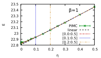
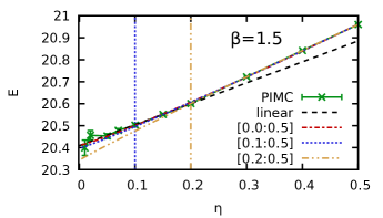
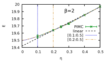
Figure 1: Convergence ($\eta$-dependence) of PIMC results for $N=6$ spin-polarized electrons in a $2D$ harmonic trap for $\lambda=0.5$ using the dipole repulsion from Eq. (14). The top, center and bottom panels show the expectation value of the original Hamiltonian $E(\eta)\equiv\braket{\hat{H}}_{\eta}$ for $\beta=1$, $\beta=1.5$ and $\beta=2$, respectively. The green crosses are PIMC expectation values, the dotted blue and dashed-double-dotted yellow curves fits according to Eq. (19) in different $\eta$-ranges, and the dashed black lines linear fits serving as a guide to the eye.

In Fig. 1, we show PIMC results for $N=6$ spin-polarized electrons in a $2D$ harmonic trap for an intermediate value of $\lambda=0.5$, and three different temperatures, $\beta=1$ (top panel), $\beta=1.5$ (center panel), and $\beta=2$ (bottom panel). The green crosses depict the PIMC results for $\braket{\hat{H}}_{\eta}$ for different values of $\eta$. First, we note that the PIMC data do monotonically converge towards the exact $\eta=0$ limit from above, as predicted by Eq. (10). For $\beta=1$, the system is substantially out of the ground-state, and we find an average sign of $S\sim 10^{-2}$ for standard PIMC (i.e., $\eta=0$), cf. Fig. 2. Hence, the PIMC simulations can be converged over the entire $\eta$-range. The dashed black line corresponds to a linear fit within the interval $\eta\in[0,0.5]$ and has been included as a guide to the eye, although we find it to be surprisingly accurate in this case. The dash-dotted red line was obtained from a fit within the same interval, but using the modified functional form

$$E(\eta)=a+b\eta^{c}\ ,$$ (19)

which has been found empirically, and with $a$, $b$, and $c$ being free parameters. Furthermore, the dotted blue and dash-double-dotted yellow lines have also been obtained from fits via Eq. (19), but within the intervals $\eta\in[0.1,0.5]$ and $\eta\in[0.2,0.5]$, respectively. Evidently, all three curves are in excellent agreement with the PIMC data over the full depicted $\eta$-range. This is an important intermediate result, as it indicates that Eq. (19) constitutes a suitable form to extrapolate results to $\eta=0$ when PIMC simulations are limited to some finite value of $\eta$ due to the sign problem.

We next examine the center panel, which corresponds to $\beta=1.5$, an intermediate temperature. In this case, we find $S\sim 10^{-3}$ for standard PIMC, which means that simulations are computationally demanding, but still feasible over the full $\eta$-range. Firstly, we note that the linear fit is not as good as for $\beta=1$ above, so we have only used data points for $\eta\in[0,0.2]$ in the linear fitting. Secondly, we find that the blue and red curves are in excellent agreement, whereas the yellow curve somewhat deviates in the limit $\eta\to 0$. Most probably, this is a consequence of the reduced fit interval of $\eta\in[0.2,0.5]$. Still, the extrapolation to $\eta=0$ agrees with the two other curves (with the red curve basically being exact) to a relative accuracy of $0.3\%$, which is sufficient for most applications. At the same time, the yellow curve requires simulations with an average sign of $S\sim 0.1$ at the lowest ($\eta=0.2$), resulting in a speed-up by a factor $T\sim 10^{3}$, see Fig. 2.

Finally, the bottom panel corresponds to $\beta=2$, where $S\sim 10^{-4}$ for standard PIMC. Thus, PIMC simulations are severely hampered by the sign problem and simulations are not feasible for $\eta\lesssim 0.1$. Still, the dotted blue ($\eta\in[0.1,0.5]$) and dash-double-dotted yellow ($\eta\in[0.2,0.5]$) curves are in very good agreement with each other, which strongly suggests that the extrapolation is reliable. Evidently, the extrapolation procedure can provide accurate results where standard PIMC simulations are prohibitive because of the sign problem.

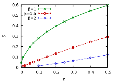
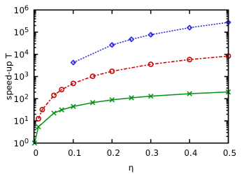
Figure 2: Dependence of the average sign $S$ (top panel) and the speed-up $T$ (bottom panel, cf. Eq. (18)) on the repulsion strength $\eta$ for $N=6$ spin-polarized electrons in a $2D$ harmonic trap for $\lambda=0.5$ using the dipole repulsion from Eq. (14). The solid green, dash-dotted red, and dotted blue curves show PIMC results for $\beta=1$, $\beta=1.5$, and $\beta=2$, respectively. Note the logarithmic scale of the $y$-axis in the bottom panel.

A quantitative analysis of the corresponding speed-up of our simulations is presented in Fig. 2. The top panel depicts results for the average sign $S(\eta)$ while the bottom panel shows the corresponding speed-up factor $T(\eta)$, as defined in Eq. (18).

The green crosses, red circles, and blue diamonds in the top panel of Fig. 2 show the $\eta$-dependence of $S$ for $\beta=1$, $\beta=1.5$, and $\beta=2$, respectively, for the same simulations reported in Fig. 1. All three data sets exhibit a qualitatively similar progression and monotonically increase with $\eta$. This growth is more pronounced for the lower temperature, $\beta=2$, where the sign increases by more than two orders of magnitude at $\eta=0.5$ as compared to $\eta=0$. Consequently, the corresponding speed-up (Fig. 2, bottom panel) is the highest for $\beta=2$ (dotted blue line), exceeding $10^{5}$ for $\eta=0.5$. From the bottom panel of Fig. 1, it is evident that simulations for $\eta\geq 0.2$, which were sufficient to obtain the energy of the original system with an accuracy of $\sim 0.1\%$ at this temperature, also provide a speed-up exceeding $10^{4}$.

For $\beta=1.5$ (dash-dotted red), the sign problem is less severe, and we find a speed-up of $T\sim 10^{3}$ for $\eta=0.1$, where no bias in the extrapolation to $\eta=0$ was resolved. Finally, the solid green line corresponds to $\beta=1$, where we find a speed-up of $T\sim 10^{2}$ for $\eta\gtrsim 0.2$.

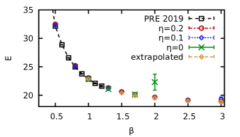
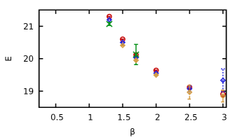
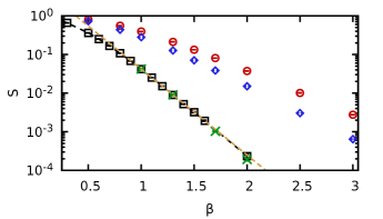
Figure 3: Temperature dependence of the energy for $N=6$ spin-polarized electrons in a $2D$ harmonic trap. The top panel shows the total energy $E$ versus $\beta$, with the following key: black squares are standard PIMC data from Ref. Dornheim (2019); green crosses are standard PIMC from this work; red circles and blue diamonds have been obtained from Eq. (10) for $\eta=0.2$ and $\eta=0.1$, respectively. The center panel shows a magnified zoom of the top panel around the lowest temperature points. The bottom panel shows the corresponding data for the average sign, with the yellow curve depicting an exponential fit according to Eq. (20). Note that the red, blue, and green data points have been obtained for the same amount of Monte Carlo samples and, thus, can be directly compared regarding efficiency.

We conclude the examination of this system by investigating the behaviour of our new approach upon decreasing the temperature. The results of this analysis are shown in Fig. 3, where the top and bottom panel show the $\beta$-dependence of the total energy $E$ and the average sign $S$. The black squares correspond to the standard PIMC data from Ref. Dornheim (2019), and accurate results for $E$ are available for $\beta\lesssim 1.3$. Data points at lower temperatures present very large error bars, and have been omitted for better visibility. Looking at $S$ itself, we find a steep decay which is of an exponential form for large $\beta$, see Eq. (6) and the corresponding analysis in Ref. Dornheim (2019). The yellow curve depicts a fit of the form

$$S(\beta)=a_{S}e^{-\beta b_{S}}\ ,$$ (20)

obtained for $\beta\in[1,3]$ and fully confirms this trend.

The green crosses in Fig. 3 represent new standard PIMC results for $\eta=0$, but obtained at a substantially increased computational cost. Therefore, results are available for $\beta\lesssim 1.5$, but at $\beta=2$ the statistical uncertainty substantially increases due to the sign problem.

We next examine the performance of our new approach based on the Bogoliubov inequality and the modified Hamiltonian from Eq. (11). The red circles and blue diamonds represent $\braket{\hat{H}}_{\eta}$ for $\eta=0.2$ and $\eta=0.1$, respectively, and the simulations can be converged down to $\beta=3$. This can be seen particularly well in the center panel of Fig. 3, showing a magnified segment around the low-temperature points. The yellow diamonds show the results which have been extrapolated to $\eta=0$ as described in the discussion of Fig. 1. These results show that our scheme allows to double the feasible $\beta$-range despite the exponential wall in compute time given by the FSP.

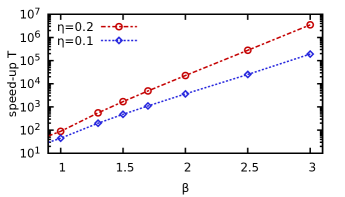
Figure 4: Relative speed-up $T$ [cf. Eq. (18)] of our simulations at $\eta=0.2$ (red circles) and $\eta=0.1$ (blue diamonds) compared to standard PIMC (i.e., $\eta=0$) for the temperature scan from Fig. 3. Note the logarithmic scale of the $y$-axis.

The speed-up $T(\eta)$ [cf. Eq. (18)] is shown in Fig. 4, with the red circles and blue diamonds depicting the $\beta$-dependence for $T(0.2)$ and $T(0.1)$, respectively. Firstly, we observe that the speed-up monotonically increases with decreasing temperature for both values of $\eta$. Moreover, this increase appears to be of an exponential form for large $\beta$, which helps to explain the remarkable extension of the parameter space that can be covered with this method. In particular, we find $T\sim 10^{6}$ ($T\sim 10^{5}$) for $\eta=0.2$ ($\eta=0.1$) for the lowest depicted temperature, $\beta=3$.

At the same time, it is important to note that this exponentially growing speed-up is still not sufficient to fully counter the sign problem, since $S$ does still monotonically (and, indeed, exponentially) decrease with $\beta$ for every fixed value of $\eta$, cf. the bottom panel of Fig. 3. Therefore, a full solution of the fermion sign problem (which we would define as a simulation scheme without an exponential increase in compute time with decreasing temperature) would require that the minimum value of $\eta$ that is needed for the extrapolation to $\eta\to 0$ increases towards low temperature. This, however, is not supported by the results of our current study.

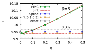
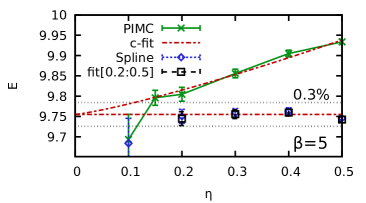
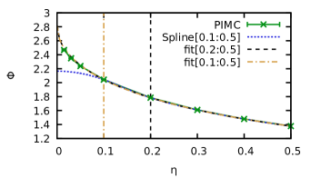
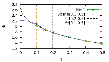
Figure 5: Results for the thermodynamic integration correction from Sec. II.3 for $N=4$ spin-polarized electrons in a $2D$ harmonic trap with $\lambda=0.5$ and $\beta=3$ (left), $\beta=5$ (right). Top row: energy estimates $E$. Bottom row: fit of $\braket{\hat{\phi}}_{\eta}$ to evaluate the integral in Eq. (16). The dashed black and dash-dotted yellow lines have been fitted according to Eq. (21), and the dash-dotted red line corresponds to a spline-fit to $\eta\braket{\hat{\phi}}_{\eta}$ for $\eta\in[0:0.5]$ (without the data point at $\eta=0.05$).

III.3 Thermodynamic integration scheme

We estimate the energy of the original system by thermodynamic integration using Eq. (16), as an alternative to extrapolation. The results are shown in the left column of Fig. 5 for $N=4$ spin-polarized electrons in a $2D$ quantum dot with $\lambda=0.5$ and $\beta=3$. The top panel shows data for the total energy $E$, and the bottom panel the expectation value $\phi(\eta)\equiv\braket{\phi}_{\eta}$, the argument of the thermodynamic integration. The green crosses depict the PIMC data for $E_{\eta}=\braket{\hat{H}}_{\eta}$ (top) and $\phi(\eta)$ (bottom), that are available at discrete $\eta$ values. Since the evaluation of Eq. (16) requires the computation of the area under $\phi(\eta^{\prime})$ for $\eta^{\prime}\in[0,\eta]$, two practical obstacles have to be overcome: i) In order to avoid performing many simulations, the computation of the integral would benefit from a continuous representation of $\phi(\eta)$ by fitting a modest number of data points and ii) we need to know $\phi(\eta)$ in the limit of small $\eta$, where PIMC simulations might no longer be feasible due to the sign problem.

Overcoming the first problem by itself is relatively easy, and the dotted blue curve in the bottom panel of Fig. 5 corresponds to a cubic spline fit to the PIMC data in the interval $\eta\in[0.1,0.5]$. The spline fit is capable to smoothly interpolate the PIMC data, but clearly fails outside the interval where input data are provided. Thus, a more controlled extrapolation to the $\eta\to 0$ limit of $\phi$ is needed for the solution to ii). We find empirically that a suitable choice is

$$\phi(\eta)=a_{\phi}+b_{\phi}\eta+c_{\phi}\eta^{1/2}\ ,$$ (21)

where $a_{\phi}$, $b_{\phi}$, and $c_{\phi}$ are the free parameters. The resulting fits are shown in Fig. 5 as the dash-dotted yellow and dashed black curves, which have been obtained taking into account PIMC data for $\eta\in[0.1,0.5]$ and $\eta\in[0.2,0.5]$, respectively.

We can see that both curves a) nicely reproduce the PIMC input data, b) are in excellent agreement with each other, and c) almost perfectly match the PIMC data that are outside of the fit interval. Therefore, the fit function Eq. (21) is capable to provide an accurate representation of $\phi(\eta)$ over the entire $\eta$-range given as input only four data points at $\eta\in[0.2,0.5]$.

Next, we use these findings to estimate the energy-correction according to Eq. (16). The results are shown in the top panel of Fig. 5, where the green crosses correspond to the uncorrected PIMC simulation data for $E_{\eta}=\braket{\hat{H}}_{\eta}$. For completeness, we also include an extrapolation of these data to $\eta=0$ according to Eq. (19, as described in Sec. III.2 (dash-dotted red line). The grey circle corresponds to a standard PIMC simulation ($\eta=0$) that is exact within the given error bars.

Using the representation of $\phi(\eta)$ according to Eq. (21) to estimate the correction leads to the yellow stars. As expected, the entire $\eta$-dependence has been removed by the correction, and the data are in perfect agreement with the exact standard PIMC results for all depicted values of $\eta$. In addition, we also show the corrected PIMC data that have been obtained by using the spline as a representation of $\phi(\eta)$ instead, see the blue diamonds in the top panel. It is important to notice that even when using such a poor extrapolation scheme, the systematic error introduced in the energy estimate is only around $0.1\%$. This shows that any error in the extrapolation of $\phi(\eta)$ will only account for a small contribution to the overall correction obtained via Eq. (16), while most of it comes from interpolation of PIMC data. This is not the case when using instead the direct extrapolation method, where any inaccuracy in the chosen functional form might more strongly impact the quality of the final result.

Finally, we mention that at the conditions considered in the left column of Fig. 5, the entropic contribution to Eq. (16) does indeed vanish within the given level of accuracy, as expected. This changes only for higher temperatures, see the discussion of Fig. 7 below.

We have also used this approach to tackle a harder example, shown in the right column of Fig. 5, where we have investigated a substantially lower temperature, $\beta=5$, for which $S\lesssim 10^{-5}$. Therefore, standard PIMC is not available in this case, and PIMC simulations are only feasible for $\eta\gtrsim 0.1$.

The bottom panel shows the estimation of $\phi(\eta)$ and, also in this case, the fits from Eq. (21) are indistinguishable for the two different intervals of input data, which substantiates the high quality of this representation. The spline, on the contrary, significantly deviates at low $\eta$ values.

The corresponding energies are shown in the top right panel of Fig. 5, and the dash-dotted red line depicts the direct extrapolation of the PIMC data to $\eta\to 0$ according to Eq. (19). In addition, the black squares and blue diamonds have been obtained from the estimation of the thermodynamic integration correction using the fit from Eq. (21) and the spline, respectively. Firstly, we find that both data sets can hardly be distinguished at these conditions, so that the extrapolation of $\phi(\eta)$ only plays a minor role for the overall level of accuracy of the energy. Secondly, the corrected energies do not exhibit any residual dependence on $\eta$ and fluctuate around the horizontal red line, with an uncertainty level of 0.1%.

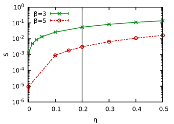
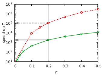
Figure 6: PIMC results for the average sign $S$ (top panel) and the respective speed-up $T$ (bottom panel) for $N=4$ spin-polarized electrons in a $2D$ harmonic trap with $\lambda=0.5$. The solid green and dash-dotted red curves correspond to $\beta=3$ and $\beta=5$, respectively. The arrows point to the speed-up for $\eta=0.2$.

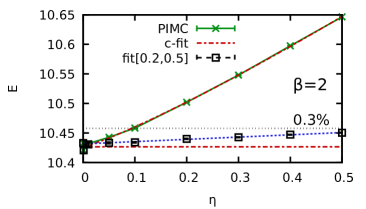
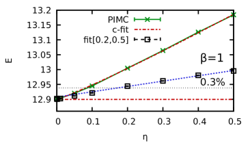
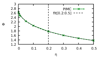
Figure 7: Results for the thermodynamic integration correction from Sec. II.3 for $N=4$ spin-polarized electrons in a $2D$ harmonic trap with $\lambda=0.5$ and $\beta=2$ (left), $\beta=1$ (right). Top row: energy estimates $E$. Bottom row: fit of $\braket{\hat{\phi}}_{\eta}$ to evaluate the integral in Eq. (16). The dashed black and dash-dotted yellow lines have been fitted according to Eq. (21), and the dash-dotted red line corresponds to a spline-fit to $\eta\braket{\hat{\phi}}_{\eta}$ for $\eta\in[0:0.5]$ (without the data point at $\eta=0.05$).

The increase of the average sign and the corresponding speed-up for both $\beta=5$ and $\beta=3$ is shown in Fig. 6. For the higher temperature (green crosses), we observe an increase in $S$ (top panel) by two order of magnitude between $\eta=0$ and $\eta=0.5$, which results in a speed-up of up to $T\sim 10^{4}$ (bottom panel). For $\beta=5$ (red circles), the relative gain in the sign is even larger, leading to a speed-up (dash-dotted red) exceeding $T\sim 10^{6}$ at the largest value of $\eta$.

A realistic application for our method performs simulations down to $\eta\gtrsim 0.2$, as this does suffice for a quasi-exact extrapolation to $\eta\to 0$. This boundary is marked as the vertical grey line in Fig. 6, and the two horizontal arrows point to the respective speed-up on the $y$-axis. For $\beta=3$, standard PIMC simulations are, in principle, possible, but our scheme results in a speed-up by a factor of $T\sim 10^{3}$. For $\beta=5$, standard PIMC is not feasible, and it is only our speed-up by a factor of $T\sim 10^{5}$ that makes it possible to obtain accurate data.

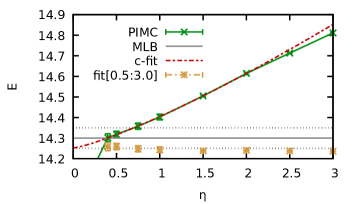
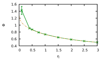
Figure 8: Results for the thermodynamic integration correction from Sec. II.3 for $N=4$ spin-polarized electrons in a $2D$ harmonic trap with $\lambda=2$ and $\beta=10$. Top panel: energy estimates $E$. The solid grey line (dotted grey line) corresponds to the MLB result (error bar) from Ref. Egger et al. (1999). Bottom panel: fit of $\braket{\hat{\phi}}_{\eta}$ to evaluate the integral in Eq. (16). The dash-double-dotted yellow line has been fitted according to Eq. (21).

For completeness, we also examine the application of the correction from Eq. (16) for higher temperatures, which is shown in Fig. 7 for $\beta=2$ (left column) and $\beta=1$ (right column). The sign problem is not severe at these parameters and we find $S\approx 0.02$ ($S\approx 0.25$) for $\beta=2$ ($\beta=1$). Thus, PIMC simulations are computationally feasible over the entire $\eta$-range for both cases. Still, we find that the functional form from Eq. (21) allows for an accurate representation of $\phi(\eta)$ (see the dashed black curve in the bottom row) taking only into account the four data points at $\eta=0.2,0.3,0.4,0.5$.

The corresponding energies are shown in the top row of Fig. 7, with the green crosses depicting the PIMC estimates for $\braket{\hat{H}}_{\eta}$, and the red curves have been obtained from a direct fit to these data according to Eq. (19). Finally, the black squares have been obtained from the thermodynamic integration correction Eq. (16). In contrast to the previous results in Fig. 7, we find a significant dependence of the corrected data points on $\eta$, which is due to the entropic contribution $\Delta S(\eta)$ to Eq. (16).

Interestingly, this function can be perfectly reproduced by a linear fit,

$$\Delta S(\eta)=a_{S}+b_{S}\eta\ ,$$ (22)

and the results are depicted by the dotted blue lines in Fig. 7.

For $\beta=2$, the entropic contribution is quite small and does not exceed $0.3\%$ even for $\eta=0.5$. In contrast, $\Delta S$ attains a maximum value of $\sim 0.7\%$ for $\beta=1$. To put these findings into the proper context, we find it useful to briefly recall the following points: i) while we cannot directly estimate $\Delta S(\eta)$ from our PIMC results, the influence on the correction from Eq. (16) decreases for low temperature, when the sign problem is most severe; ii) even when $\Delta S(\eta)$ does have an impact on the corrected energies, the residual dependence on the parameter $\eta$ is much smaller than the direct dependence of $\braket{\hat{H}}_{\eta}$, which makes a potential extrapolation to $\eta\to 0$ much less uncontrolled; iii) empirically, we find a simple linear dependence of $\Delta S$ on $\eta$, which is an additional advantage over the direct extrapolation of the uncorrected energy, where the functional dependence is more complicated, cf. Sec. III.2.

We thus conclude that the correction introduced in Sec. II.3 using thermodynamic integration constitutes a distinct improvement over the direct extrapolation explored in Sec. III.2.

We conclude this section with an application of the correction approach at higher $\lambda$ and lower temperature. In Fig. 8, we show PIMC results for the energy (top panel) and $\phi$ (bottom panel) for $N=4$ spin-polarized electrons at $\lambda=2$ and $\beta=10$. First, we mention that standard PIMC is not available at these conditions, and the sign vanishes within a statistical uncertainty of $10^{-5}$. We have chosen this particular set of parameters because it was previously studied by Egger et al. Egger et al. (1999) using the approximate multi-level blocking (MLB) method EGGER and MAK (2001); Mak et al. (1998); Dikovsky and Mak (2001). While being potentially biased Schoof (2016), such a data point still constitutes a valuable reference for the development of a new method.

As usual, the PIMC results for $\braket{\hat{H}}_{\eta}$ are depicted as the green crosses, and the dash-dotted red curve corresponds to a direct extrapolation of these data according to Eq. (19). The solid grey horizontal line depicts the MLB value from Ref. Egger et al. (1999), and the two light dotted grey lines depict the corresponding statistical uncertainty, which is given by $\Delta E/E\approx 0.35\%$. Evidently, the direct extrapolation of our data falls into the bottom of the uncertainty interval from the MLB method.

We next consider the thermodynamic integration correction, for which we need a representation of $\phi(\eta)$, shown in the bottom panel of Fig. 8. The dash-double-dotted yellow curve has been obtain using Eq. (21) as a fit function for the PIMC data, which was empirically shown to be accurate over the entire relevant $\eta$-range, see above. Using this representation to evaluate Eq. (16) results in the yellow stars in the top panel.

Firstly, we note that these data do not exhibit any residual dependence on $\eta$, as the entropic contribution is negligible at such a low temperature. Moreover, we find that the yellow stars are in excellent agreement to the result from the direct extrapolation of the PIMC data, and, thus, also in agreement within the given uncertainty interval of the MLB results.

Therefore, both the MLB method and our new approach have been successfully validated against each other for this system.

III.4 Electrons in a 3D quantum dot

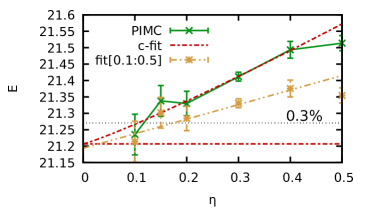
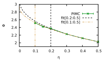
Figure 9: Top: Convergence ($\eta$-dependence) of PIMC results for $N=6$ spin-polarized electrons in a $3D$ harmonic confinement with $\lambda=0.5$ and $\beta=2$. The green crosses depict PIMC data for $E_{\eta}=\braket{\hat{H}}_{\eta}$ and the dash-dotted red line a fit according to Eq. (19). The yellow stars have been obtained using the thermodynamic integration correction from Eq. (16), and the dashed-double-dotted yellow line an extrapolation of the entropic contribution, cf. Eq. (22). Bottom: PIMC data for $\phi$ (green crosses) and fits via Eq. (21) (dashed black and dashed-double-dotted yellow) for two different $\eta$-ranges.

The final example to be investigated in this work is the application of our method to a $3D$ system. This is shown in Fig. 9 for $N=6$ electrons in a $3D$ harmonic confinement for $\lambda=0.5$ and $\beta=2$. As before, the green crosses depict the raw PIMC data for $\braket{\hat{H}}_{\eta}$ and the dash-dotted red-line a direct extrapolation thereof according to Eq. (19). At these conditions, we find an average sign of $S\sim 10^{-4}$ [cf. Fig. 10], which means that standard PIMC simulations are only feasible for $\eta\gtrsim 0.1$. Yet, the fit function from Eq. (19) evidently allows for a controlled extrapolation to $\eta\to 0$, which is further highlighted by the dotted light grey horizontal line, depicting an uncertainty interval of $0.3\%$ around the extrapolated value.

We next explore the estimation of the thermodynamic integration correction introduced in Sec. II.3. To this end, we show $\phi(\eta)$ in the bottom panel of Fig. 9 and the green crosses again show the PIMC data. The dashed black (dashed-double-dotted yellow) line corresponds to a fit using the functional form from Eq. (21) for $\eta\in[0.2,0.5]$ ($\eta\in[0.1,0.5]$). Naturally, these representations are in excellent agreement for large $\eta$, whereas some deviations appear for the extrapolation of $\eta\to 0$.

Using one of these representations as input to evaluate the thermodynamic integration correction from Eq. (16) gives the yellow stars (Eq. (21) for $\eta\in[0.1,0.5]$. For completeness, we mention that even using a spline-representation of $\phi(\eta)$ would result in almost indistinguishable energy values, which further validates the observation from the previous Sec. III.3 that the particular extrapolation of $\phi(\eta)$ to $\eta\to 0$ hardly influence the quality of the corrected energies. At the same time, we observe a distinct entropic contribution to Eq. (16) at these conditions, and the dashed-double-dotted yellow line corresponds to a linear fit to the corrected data points, cf. Eq. (22). Evidently, the linear representation is in perfect agreement to the yellow stars over the entire depicted $\eta$-range, and the $\eta\to 0$ limit nicely agrees with the direct extrapolation of the uncorrected PIMC data points.

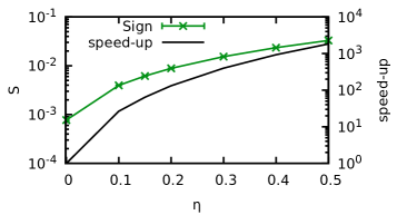
Figure 10: Dependence of the average sign $S$ (green crosses, left $y$-axis) and the speed-up T (cf. Eq. (18), solid black line, right $y$-axis) on the repulsion strength $\eta$ for $N=6$ spin-polarized electrons in a $3D$ harmonic trap for $\lambda=0.5$ and $\beta=2$.

We conclude this section with an analysis of the average sign $S$ and the corresponding speed-up $T$ [cf. Eq. (18)], shown in Fig. 10. The green crosses show the PIMC data for $S$ (left $y$-axis) and exhibit a monotonic increase similar to the $2D$ case. Further, the respective speed-up is depicted as the solid black curve (right $y$-axis) and attains values exceeding $T=10^{3}$ for $\eta=0.5$.

IV Summary and Discussion

We present a new approach for PIMC simulations of fermions at finite temperature, that extends and improves the idea by Hirshberg et al. Hirshberg et al. (2020), that was based on the Bogoliubov inequality. We add to the Hamiltonian a repulsive term that mimics Pauli repulsion at short range and is proportional to a coupling parameter $\eta$. This significantly improves the efficiency of the simulations, by increasing the average sign $S$. We then propose two simple post-processing schemes to recover the energy of the original system. The first one is based on the Bogoliubov inequality and consists of extrapolating $\braket{\hat{H}}_{\eta}$ obtained for various values of $\eta$ to the limit $\eta\to 0$. The second one instead is based on thermodynamic integration and also relies on an extrapolation, but only of the perturbation term $\phi$ and not of the whole energy. Combined with the fact that it is based on an exact relation and not an inequality, this makes the second scheme generally more reliable. We believe that having two distinct schemes for evaluating the energy, starting from the same simulations, is a great advantage, and makes the method more robust against possible poor extrapolation choices. For all the systems considered here, the two schemes provided compatible energy estimates. Most importantly, they allowed evaluating accurate estimates of energies for conditions in which standard PIMC simulations were not feasible.

As a practical application, we have investigated electrons both in $2D$ and $3D$ quantum dots, and our method works very well in both of these cases. In particular, we have found that a direct extrapolation by itself allows for a speed-up of up to $10^{6}$ (cf. Fig. 4), while retaining a relative accuracy of $0.1\%$, which is fully sufficient for practical purposes. This, in turn, allows to double the feasible $\beta$-range as compared to standard PIMC.

The investigation of the thermodynamic integration correction introduced in Sec. II.3 has revealed that this approach makes the estimation of the energy of the original system even more reliable. Here, the main challenge is given by the construction of a representation of $\phi(\eta)$ with no data points being available below some minimum value. As a solution, we have introduced a suitable empirical fit function [cf. Eq. (21)] that, remarkably, allows for a highly reliable extrapolation using only a few data points at large $\eta$ as input. At low temperature, this representation allows to accurately estimate the energy of the original system of interest. For higher temperatures, there emerges an additional entropic contribution, which remains a priori unknown. Still, we stress that the latter only constitutes a fraction of the full difference between the modified and the original system, and, empirically, exhibits a linear dependence on $\eta$ (cf. Fig. 7).

While the present results are certainly encouraging, much can be done to improve the method further. From a technical point of view, implementing the sampling procedure proposed in Ref. 89 would make the method more efficient, requiring only a single simulation for estimating $E(\eta)$ and $\phi(\eta)$ in the whole range of $\eta$ values. Furthermore, we mention that, despite a speed-up of $10^{6}$, the fermion sign problem has not been completely removed and, while our approach significantly extends the range of accessible parameters, it still suffers from exponential increase in computing time at low enough temperatures. We have also restricted ourselves to the investigation of energy values, and the adaption of the method to other observables such as pair distributions, structure factors, or the different contributions to $E$ like the kinetic or external potential energies is of high interest. Similarly, we have solely used a dipolar repulsive potential $\Psi(r_{1},r_{2})$ and the optimization of $\Psi$ might substantially improve the approach.

A particularly interesting topic for future research is given by the application to other systems, with warm-dense matter Bonitz et al. (2020) being a promising candidate. Finally, we stress that our approach is quite general and can readily be adapted to other simulation methods for fermions both in the ground state and at finite temperate.

References

- Giuliani and Vignale (2008) G. Giuliani and G. Vignale, Quantum Theory of the Electron Liquid (Cambridge University Press, Cambridge, 2008).
- Loh et al. (1990) E. Y. Loh, J. E. Gubernatis, R. T. Scalettar, S. R. White, D. J. Scalapino, and R. L. Sugar, “Sign problem in the numerical simulation of many-electron systems,” Phys. Rev. B 41, 9301–9307 (1990).
- Troyer and Wiese (2005) M. Troyer and U. J. Wiese, “Computational complexity and fundamental limitations to fermionic quantum Monte Carlo simulations,” Phys. Rev. Lett 94, 170201 (2005).
- Dornheim (2019) T. Dornheim, “Fermion sign problem in path integral Monte Carlo simulations: Quantum dots, ultracold atoms, and warm dense matter,” Phys. Rev. E 100, 023307 (2019).
- Ceperley and Alder (1980) D. M. Ceperley and B. J. Alder, “Ground state of the electron gas by a stochastic method,” Phys. Rev. Lett. 45, 566–569 (1980).
- Perdew and Zunger (1981) J. P. Perdew and Alex Zunger, “Self-interaction correction to density-functional approximations for many-electron systems,” Phys. Rev. B 23, 5048–5079 (1981).
- Perdew et al. (1996) John P Perdew, Kieron Burke, and Matthias Ernzerhof, “Generalized gradient approximation made simple,” Physical Review Letters 77, 3865 (1996).
- Burke (2012) Kieron Burke, “Perspective on density functional theory,” The Journal of Chemical Physics 136, 150901 (2012), https://doi.org/10.1063/1.4704546 .
- Ceperley (1991) D. M. Ceperley, “Fermion nodes,” Journal of Statistical Physics 63, 1237–1267 (1991).
- Anderson (1995) James B. Anderson, “Fixed-node quantum monte carlo,” International Reviews in Physical Chemistry 14, 85–112 (1995), https://doi.org/10.1080/01442359509353305 .
- Foulkes et al. (2001) W. M. C. Foulkes, L. Mitas, R. J. Needs, and G. Rajagopal, “Quantum monte carlo simulations of solids,” Rev. Mod. Phys. 73, 33–83 (2001).
- López Ríos et al. (2006) P. López Ríos, A. Ma, N. D. Drummond, M. D. Towler, and R. J. Needs, “Inhomogeneous backflow transformations in quantum monte carlo calculations,” Phys. Rev. E 74, 066701 (2006).
- Needs et al. (2009) R J Needs, M D Towler, N D Drummond, and P López Ríos, “Continuum variational and diffusion quantum monte carlo calculations,” Journal of Physics: Condensed Matter 22, 023201 (2009).
- Booth et al. (2009) George H. Booth, Alex J. W. Thom, and Ali Alavi, “Fermion monte carlo without fixed nodes: A game of life, death, and annihilation in slater determinant space,” The Journal of Chemical Physics 131, 054106 (2009), https://aip.scitation.org/doi/pdf/10.1063/1.3193710 .
- Honma et al. (1995) Michio Honma, Takahiro Mizusaki, and Takaharu Otsuka, “Diagonalization of hamiltonians for many-body systems by auxiliary field quantum monte carlo technique,” Phys. Rev. Lett. 75, 1284–1287 (1995).
- Motta and Zhang (2018) Mario Motta and Shiwei Zhang, “Ab initio computations of molecular systems by the auxiliary-field quantum monte carlo method,” WIREs Computational Molecular Science 8, e1364 (2018), https://onlinelibrary.wiley.com/doi/pdf/10.1002/wcms.1364 .
- LeBlanc et al. (2015) J. P. F. LeBlanc, Andrey E. Antipov, Federico Becca, Ireneusz W. Bulik, Garnet Kin-Lic Chan, Chia-Min Chung, Youjin Deng, Michel Ferrero, Thomas M. Henderson, Carlos A. Jiménez-Hoyos, E. Kozik, Xuan-Wen Liu, Andrew J. Millis, N. V. Prokof’ev, Mingpu Qin, Gustavo E. Scuseria, Hao Shi, B. V. Svistunov, Luca F. Tocchio, I. S. Tupitsyn, Steven R. White, Shiwei Zhang, Bo-Xiao Zheng, Zhenyue Zhu, and Emanuel Gull (Simons Collaboration on the Many-Electron Problem), “Solutions of the two-dimensional hubbard model: Benchmarks and results from a wide range of numerical algorithms,” Phys. Rev. X 5, 041041 (2015).
- Booth et al. (2013) George H. Booth, Andreas Grüneis, Georg Kresse, and Ali Alavi, “Towards an exact description of electronic wavefunctions in real solids,” Nature 493, 365–370 (2013).
- Brown et al. (2013) Ethan W. Brown, Bryan K. Clark, Jonathan L. DuBois, and David M. Ceperley, “Path-integral monte carlo simulation of the warm dense homogeneous electron gas,” Phys. Rev. Lett. 110, 146405 (2013).
- Schoof et al. (2011) T. Schoof, M. Bonitz, A. Filinov, D. Hochstuhl, and J.W. Dufty, “Configuration path integral monte carlo,” Contributions to Plasma Physics 51, 687–697 (2011).
- Dornheim et al. (2015a) Tobias Dornheim, Simon Groth, Alexey Filinov, and Michael Bonitz, “Permutation blocking path integral monte carlo: a highly efficient approach to the simulation of strongly degenerate non-ideal fermions,” New Journal of Physics 17, 073017 (2015a).
- Dornheim et al. (2017) Tobias Dornheim, Simon Groth, Fionn D. Malone, Tim Schoof, Travis Sjostrom, W. M. C. Foulkes, and Michael Bonitz, “Ab initio quantum monte carlo simulation of the warm dense electron gas,” Physics of Plasmas 24, 056303 (2017), https://doi.org/10.1063/1.4977920 .
- Blunt et al. (2014) N. S. Blunt, T. W. Rogers, J. S. Spencer, and W. M. C. Foulkes, “Density-matrix quantum monte carlo method,” Phys. Rev. B 89, 245124 (2014).
- Liu et al. (2018) Yuan Liu, Minsik Cho, and Brenda Rubenstein, “Ab initio finite temperature auxiliary field quantum monte carlo,” Journal of Chemical Theory and Computation 14, 4722–4732 (2018).
- Malone et al. (2015) Fionn D. Malone, N. S. Blunt, James J. Shepherd, D. K. K. Lee, J. S. Spencer, and W. M. C. Foulkes, “Interaction picture density matrix quantum monte carlo,” The Journal of Chemical Physics 143, 044116 (2015), https://doi.org/10.1063/1.4927434 .
- Malone et al. (2016) Fionn D. Malone, N. S. Blunt, Ethan W. Brown, D. K. K. Lee, J. S. Spencer, W. M. C. Foulkes, and James J. Shepherd, “Accurate exchange-correlation energies for the warm dense electron gas,” Phys. Rev. Lett. 117, 115701 (2016).
- Claes and Clark (2017) Jahan Claes and Bryan K. Clark, “Finite-temperature properties of strongly correlated systems via variational monte carlo,” Phys. Rev. B 95, 205109 (2017).
- Dornheim et al. (2019a) Tobias Dornheim, Simon Groth, and Michael Bonitz, “Permutation blocking path integral monte carlo simulations of degenerate electrons at finite temperature,” Contributions to Plasma Physics 59, e201800157 (2019a), https://onlinelibrary.wiley.com/doi/pdf/10.1002/ctpp.201800157 .
- Yilmaz et al. (2020) A. Yilmaz, K. Hunger, T. Dornheim, S. Groth, and M. Bonitz, “Restricted configuration path integral monte carlo,” (2020), arXiv:2007.12498 [physics.comp-ph] .
- Dornheim et al. (2020a) Tobias Dornheim, Jan Vorberger, and Michael Bonitz, “Nonlinear electronic density response in warm dense matter,” Phys. Rev. Lett. 125, 085001 (2020a).
- Driver et al. (2018) K. P. Driver, F. Soubiran, and B. Militzer, “Path integral monte carlo simulations of warm dense aluminum,” Phys. Rev. E 97, 063207 (2018).
- Dornheim et al. (2018a) T. Dornheim, S. Groth, J. Vorberger, and M. Bonitz, “Ab initio path integral Monte Carlo results for the dynamic structure factor of correlated electrons: From the electron liquid to warm dense matter,” Phys. Rev. Lett. 121, 255001 (2018a).
- Graziani et al. (2014) F. Graziani, M. P. Desjarlais, R. Redmer, and S. B. Trickey, eds., Frontiers and Challenges in Warm Dense Matter (Springer, International Publishing, 2014).
- Bonitz et al. (2020) M. Bonitz, T. Dornheim, Zh. A. Moldabekov, S. Zhang, P. Hamann, H. Kählert, A. Filinov, K. Ramakrishna, and J. Vorberger, “Ab initio simulation of warm dense matter,” Physics of Plasmas 27, 042710 (2020).
- Dornheim et al. (2018b) T. Dornheim, S. Groth, and M. Bonitz, “The uniform electron gas at warm dense matter conditions,” Phys. Reports 744, 1–86 (2018b).
- Fortov (2009) V. E. Fortov, “Extreme states of matter on earth and in space,” Phys.-Usp 52, 615–647 (2009).
- Pribram-Jones et al. (2014) Aurora Pribram-Jones, Stefano Pittalis, E. K. U. Gross, and Kieron Burke, “Thermal Density Functional Theory in Context,” (2014) pp. 25–60.
- Smith et al. (2018) Justin C. Smith, Francisca Sagredo, and Kieron Burke, “Warming Up Density Functional Theory,” in Frontiers of Quantum Chemistry (Springer Singapore, Singapore, 2018) pp. 249–271.
- Cytter et al. (2018) Yael Cytter, Eran Rabani, Daniel Neuhauser, and Roi Baer, “Stochastic density functional theory at finite temperatures,” Phys. Rev. B 97, 115207 (2018).
- Karasiev et al. (2016) V. V. Karasiev, L. Calderin, and S. B. Trickey, “Importance of finite-temperature exchange correlation for warm dense matter calculations,” Phys. Rev. E 93, 063207 (2016).
- Ramakrishna et al. (2020) Kushal Ramakrishna, Tobias Dornheim, and Jan Vorberger, “Influence of finite temperature exchange-correlation effects in hydrogen,” Phys. Rev. B 101, 195129 (2020).
- Dornheim et al. (2016a) T. Dornheim, S. Groth, T. Sjostrom, F. D. Malone, W. M. C. Foulkes, and M. Bonitz, “Ab initio quantum Monte Carlo simulation of the warm dense electron gas in the thermodynamic limit,” Phys. Rev. Lett. 117, 156403 (2016a).
- Groth et al. (2017) S. Groth, T. Dornheim, T. Sjostrom, F. D. Malone, W. M. C. Foulkes, and M. Bonitz, “Ab initio exchange–correlation free energy of the uniform electron gas at warm dense matter conditions,” Phys. Rev. Lett. 119, 135001 (2017).
- Dornheim (2020) Tobias Dornheim, “Path-integral monte carlo simulations of quantum dipole systems in traps: Superfluidity, quantum statistics, and structural properties,” Phys. Rev. A 102, 023307 (2020).
- Filinov (2016) A. Filinov, “Correlation effects and collective excitations in bosonic bilayers: Role of quantum statistics, superfluidity, and the dimerization transition,” Phys. Rev. A 94, 013603 (2016).
- Schleede et al. (2012) J. Schleede, A. Filinov, M. Bonitz, and H. Fehske, “Phase diagram of bilayer electron-hole plasmas,” Contributions to Plasma Physics 52, 819–826 (2012), https://onlinelibrary.wiley.com/doi/pdf/10.1002/ctpp.201200045 .
- Dornheim et al. (2016b) T. Dornheim, H. Thomsen, P. Ludwig, A. Filinov, and M. Bonitz, “Analyzing quantum correlations made simple,” Contributions to Plasma Physics 56, 371–379 (2016b), https://onlinelibrary.wiley.com/doi/pdf/10.1002/ctpp.201500120 .
- Kylänpää and Räsänen (2017) Ilkka Kylänpää and Esa Räsänen, “Path integral monte carlo benchmarks for two-dimensional quantum dots,” Phys. Rev. B 96, 205445 (2017).
- Egger et al. (1999) R. Egger, W. Häusler, C. H. Mak, and H. Grabert, “Crossover from fermi liquid to wigner molecule behavior in quantum dots,” Phys. Rev. Lett. 82, 3320–3323 (1999).
- EGGER and MAK (2001) R. EGGER and C. H. MAK, “Multilevel blocking monte carlo simulations for quantum dots,” International Journal of Modern Physics B 15, 1416–1425 (2001), https://doi.org/10.1142/S021797920100591X .
- Filinov et al. (2001) A. V. Filinov, M. Bonitz, and Yu. E. Lozovik, “Wigner crystallization in mesoscopic 2d electron systems,” Phys. Rev. Lett. 86, 3851–3854 (2001).
- Filinov et al. (2013) V. S. Filinov, Yu. B. Ivanov, V. E. Fortov, M. Bonitz, and P. R. Levashov, “Color path-integral monte-carlo simulations of quark-gluon plasma: Thermodynamic and transport properties,” Phys. Rev. C 87, 035207 (2013).
- Filinov et al. (2015) V.S. Filinov, M. Bonitz, Y.B. Ivanov, E.-M. Ilgenfritz, and V.E. Fortov, “Thermodynamics of the quark-gluon plasma at finite chemical potential: Color path integral monte carlo results,” Contributions to Plasma Physics 55, 203–208 (2015), https://onlinelibrary.wiley.com/doi/pdf/10.1002/ctpp.201400056 .
- Yan and Blume (2014) Yangqian Yan and D. Blume, “Abnormal superfluid fraction of harmonically trapped few-fermion systems,” Phys. Rev. Lett. 112, 235301 (2014).
- Filinov et al. (2000) A.V. Filinov, Yu.E. Lozovik, and M. Bonitz, “Path integral simulations of crystallization of quantum confined electrons,” physica status solidi (b) 221, 231–234 (2000).
- Zenker et al. (2012) B. Zenker, D. Ihle, F. X. Bronold, and H. Fehske, “Electron-hole pair condensation at the semimetal-semiconductor transition: A bcs-bec crossover scenario,” Phys. Rev. B 85, 121102 (2012).
- Ohashi and Griffin (2002) Y. Ohashi and A. Griffin, “Bcs-bec crossover in a gas of fermi atoms with a feshbach resonance,” Phys. Rev. Lett. 89, 130402 (2002).
- Groth et al. (2019) S. Groth, T. Dornheim, and J. Vorberger, “Ab initio path integral Monte Carlo approach to the static and dynamic density response of the uniform electron gas,” Phys. Rev. B 99, 235122 (2019).
- Dornheim et al. (2020b) Tobias Dornheim, Zhandos A Moldabekov, Jan Vorberger, and Simon Groth, “Ab initio path integral monte carlo simulation of the uniform electron gas in the high energy density regime,” Plasma Physics and Controlled Fusion 62, 075003 (2020b).
- Hamann et al. (2020) Paul Hamann, Tobias Dornheim, Jan Vorberger, Zhandos A. Moldabekov, and Michael Bonitz, “Dynamic properties of the warm dense electron gas: an ab initio path integral monte carlo approach,” (2020), arXiv:2007.15471 [physics.comp-ph] .
- Karasiev et al. (2019) V. V. Karasiev, S. B. Trickey, and J. W. Dufty, “Status of free-energy representations for the homogeneous electron gas,” Phys. Rev. B 99, 195134 (2019).
- Ceperley (1995) D. M. Ceperley, “Path integrals in the theory of condensed helium,” Rev. Mod. Phys 67, 279 (1995).
- Verbeure (2010) A.F. Verbeure, Many-Body Boson Systems: Half a Century Later, Theoretical and Mathematical Physics (Springer London, 2010).
- Hirshberg et al. (2020) Barak Hirshberg, Michele Invernizzi, and Michele Parrinello, “Path integral molecular dynamics for fermions: Alleviating the sign problem with the bogoliubov inequality,” The Journal of Chemical Physics 152, 171102 (2020), https://doi.org/10.1063/5.0008720 .
- Hirshberg et al. (2019) Barak Hirshberg, Valerio Rizzi, and Michele Parrinello, “Path integral molecular dynamics for bosons,” Proceedings of the National Academy of Sciences 116, 21445–21449 (2019), https://www.pnas.org/content/116/43/21445.full.pdf .
- Frenkel and Smit (2001) Daan Frenkel and Berend Smit, Understanding Molecular Simulation: from algorithms to applications (Academic Press, 2001) p. 664.
- De Raedt and De Raedt (1983) Hans De Raedt and Bart De Raedt, “Applications of the generalized trotter formula,” Phys. Rev. A 28, 3575–3580 (1983).
- Metropolis et al. (1953) Nicholas Metropolis, Arianna W. Rosenbluth, Marshall N. Rosenbluth, Augusta H. Teller, and Edward Teller, “Equation of state calculations by fast computing machines,” The Journal of Chemical Physics 21, 1087–1092 (1953), https://doi.org/10.1063/1.1699114 .
- Dornheim et al. (2019b) T. Dornheim, S. Groth, A. V. Filinov, and M. Bonitz, “Path integral monte carlo simulation of degenerate electrons: Permutation-cycle properties,” The Journal of Chemical Physics 151, 014108 (2019b).
- Boninsegni et al. (2006a) M. Boninsegni, N. V. Prokofev, and B. V. Svistunov, “Worm algorithm and diagrammatic Monte Carlo: A new approach to continuous-space path integral Monte Carlo simulations,” Phys. Rev. E 74, 036701 (2006a).
- Boninsegni et al. (2006b) M. Boninsegni, N. V. Prokofev, and B. V. Svistunov, “Worm algorithm for continuous-space path integral Monte Carlo simulations,” Phys. Rev. Lett 96, 070601 (2006b).
- Filinov et al. (2010) A. Filinov, N. V. Prokof’ev, and M. Bonitz, “Berezinskii-kosterlitz-thouless transition in two-dimensional dipole systems,” Phys. Rev. Lett. 105, 070401 (2010).
- Boninsegni and Prokof’ev (2012) Massimo Boninsegni and Nikolay V. Prokof’ev, “Colloquium: Supersolids: What and where are they?” Rev. Mod. Phys. 84, 759–776 (2012).
- Dornheim et al. (2015b) T. Dornheim, A. Filinov, and M. Bonitz, “Superfluidity of strongly correlated bosons in two- and three-dimensional traps,” Phys. Rev. B 91, 054503 (2015b).
- Pollet et al. (2007) L. Pollet, M. Boninsegni, A. B. Kuklov, N. V. Prokof’ev, B. V. Svistunov, and M. Troyer, “Superfluidity of grain boundaries in solid ,” Phys. Rev. Lett. 98, 135301 (2007).
- Boninsegni and Ceperley (1996) Massimo Boninsegni and David M. Ceperley, “Density fluctuations in liquid4he. path integrals and maximum entropy,” Journal of Low Temperature Physics 104, 339–357 (1996).
- Filinov and Bonitz (2012) A. Filinov and M. Bonitz, “Collective and single-particle excitations in two-dimensional dipolar bose gases,” Phys. Rev. A 86, 043628 (2012).
- Dornheim and Vorberger (2020) Tobias Dornheim and Jan Vorberger, “Finite-size effects in the reconstruction of dynamic properties from ab initio path integral Monte-Carlo simulations,” arXiv e-prints , arXiv:2004.13429 (2020), arXiv:2004.13429 [cond-mat.str-el] .
- Kora and Boninsegni (2018) Youssef Kora and Massimo Boninsegni, “Dynamic structure factor of superfluid from quantum monte carlo: Maximum entropy revisited,” Phys. Rev. B 98, 134509 (2018).
- Groth et al. (2016) S. Groth, T. Schoof, T. Dornheim, and M. Bonitz, “Ab initio quantum monte carlo simulations of the uniform electron gas without fixed nodes,” Phys. Rev. B 93, 085102 (2016).
- Prokof’ev and Svistunov (2008) Nikolay Prokof’ev and Boris Svistunov, “Fermi-polaron problem: Diagrammatic monte carlo method for divergent sign-alternating series,” Phys. Rev. B 77, 020408 (2008).
- Ellenberger et al. (2006) C. Ellenberger, T. Ihn, C. Yannouleas, U. Landman, K. Ensslin, D. Driscoll, and A. C. Gossard, “Excitation spectrum of two correlated electrons in a lateral quantum dot with negligible zeeman splitting,” Phys. Rev. Lett. 96, 126806 (2006).
- Mezzacapo and Boninsegni (2007) F. Mezzacapo and M. Boninsegni, “Structure, superfluidity, and quantum melting of hydrogen clusters,” Phys. Rev. A 75, 033201 (2007).
- Sakkos et al. (2009) K. Sakkos, J. Casulleras, and J. Boronat, “High order chin actions in path integral monte carlo,” The Journal of Chemical Physics 130, 204109 (2009), https://doi.org/10.1063/1.3143522 .
- Brualla et al. (2004) L. Brualla, K. Sakkos, J. Boronat, and J. Casulleras, “Higher order and infinite trotter-number extrapolations in path integral monte carlo,” The Journal of Chemical Physics 121, 636–643 (2004), https://doi.org/10.1063/1.1760512 .
- Mak et al. (1998) C. H. Mak, R. Egger, and H. Weber-Gottschick, “Multilevel blocking approach to the fermion sign problem in path-integral monte carlo simulations,” Phys. Rev. Lett. 81, 4533–4536 (1998).
- Dikovsky and Mak (2001) Mikhail V. Dikovsky and C. H. Mak, “Analysis of the multilevel blocking approach to the fermion sign problem: Accuracy, errors, and practice,” Phys. Rev. B 63, 235105 (2001).
- Schoof (2016) Tim Schoof, Configuration Path Integral Monte Carlo: Ab initio simulations of fermions in the warm dense matter regime, Ph.D. thesis, Christian-Albrechts-Universität zu Kiel, Kiel, Germany (2016).
- Invernizzi et al. (2020) Michele Invernizzi, Pablo M. Piaggi, and Michele Parrinello, “A Unified Approach to Enhanced Sampling,” arXiv e-prints (2020), arXiv:2007.03055 .