Response to referee reports on the Manuscript (Ref. No. JFEC-2018-006 ) ”Pricing Cryptocurrency options”

We are grateful that the Editor and the Referees have provided us with such helpful and constructive comments and suggestions. Below we explain in detail and with care for each of the valuable comments. The original comments are in italic and they are followed by our response.

1. Editor
   

   1. The fundamental issue with the current draft is lack of tightness. All you need to do - at this juncture - is provide a crispier product, one which does not indulge in undocumented statements and is detailed on what is new.
      

      We have revised accordingly and specified clearly what is new in the introduction. We have revised according to the AE’s suggestions and the revised verison is much tightener than the last version.
      

   2. I recommend that you follow closely the recommendations of the AE.
      

      We have closely followed the AE’s suggestions and carefully addressed all comments from the AE. Below please find a point-by-point answer.
      

   3. While I agree with the AE that the ARIMA/GARCH portion of the paper reads as being contrived, there has to be a less scholastic way to provide descriptive information about Bitcoin dynamics before getting into continuous-time modelling. I would be in favour of having such an analysis in the paper. Again, it would simply amount to a less scholastic version of what you already have. .
      

      We agree with you and the AE. We have provided a very short and less scholastic way of describing the BTC price dynamics, see Section 2, Page 5, 6. Moreover, we have tightly follow the suggestion of AE and move the ARIMA and the GARCH parts to the Appendix.
      

   4. In the spirit of publishing a crispier product, I would personally change the title of the paper to ”Pricing cryptocurrency options.”
      

      Thanks, the title of the paper has been changed to ”Pricing cryptocurrency options.”
      

   5. As for keeping CRIX in the paper, I do not mind having a robustness section provided it is informative, even from an institutional standpoint. Given the structure of the index, should we expect large deviations from Bitcoin dynamics? What is the correlation between CRIX and Bitcoins? Discuss the difference between bitcoin and the CRIX, focusing on the institutional points of view
      

      Bitcoin is the leading cryptocurrency and plays a major role in the composite cryptocurrency index. The correlation between Bitcoin and CRIX in our sample period is around 0.91. With such high correlation, one should not expect a high deviation between their dynamics. However, Bitcoin alone cannot represent the cryptocurrency market as a whole. Especially, from the institutional investors’ perspective, the portfolio like CRIX yields a higher Sharpe ratio than Bitcoins does. More details can be found on Page 26-28, in Section 6.
      

   6. Depending on the quality of the revision, I may decide not to send the paper out to reviewers upon resubmission
      

      We have revised the paper tightly followed the AE’s suggestions as well as all points addressed by the referee (besides point 3 of the referee, as we agree with AE, this point is too ambitious to our current paper and we would leave this point to a future research.
      

2. Associate Editor

   In my previous report, I wrote that the writing of the paper needed a lot of work. I also asked for a clarification of why the different parts of the paper (ARIMA and SV models) were not better integrated. In response, the authors seem to have done a fair amount of work, but the paper is still not in very good shape, in my view. In this report, I will try to give more specific suggestions. .
   

   First, I would drop the ARIMA models. As the authors note, the results here are of marginal statistical significance. Furthermore, even this marginal significance is somewhat suspect. Autocorrelations are negative at some lags and positive at others. The method of computing standard errors is not reported, but the numbers look like they may not be robust. And lastly, as the authors show in their reply to my first report, these patterns in the conditional mean are completely irrelevant for the analysis in the later sections on SV models.
   

   We agree with the AE, and the ARIMA model has been moved from the paper to the Appendix.
   

   Second, I would drop the GARCH models. The results here are redundant in two ways. First, there are already many papers that study GARCH models in cryptocurrencies. Second, GARCH effects are also present in the SV models considered later in the paper. I just don’t see a contribution here.
   

   We agree with the AE, and the GARCH model has been moved from the paper to the Appendix.
   

   Third, I would drop the CRIX estimation results. I don’t think they are worth including due to their similarity with Bitcoin results. With this material eliminated, the focus will be on the more interesting and novel results in the paper. These sections can also be improved.
   

   We have moved all the estimation results of the CRIX part to the appendix. Furthermore, following the suggestions from the editor, we discuss CRIX particularly from the institutional investors’ perspective in Section 6.
   

   Here is a list of suggestions:
   

   1. On page 3, the paper states that Conventional financial or economic theories may fail to embrace this new asset class. I don’t know what this means. The sentence if vague, and the word ”embrace” is out of context.
      

      We have dropped this sentence from the introduction to avoid possible confusions.
      

   2. Also on page 3, the paper states that ”The pricing of contingent claims may not be easily adapted for the crypto market since the frequent appearance of jumps in addition to stochastic volatility behavior makes the markets incomplete.” Yet the paper is adapting off-the-shelf models with SV and jumps. There would appear to be no difficulties that arise as a result of applying these models to crypto assets.
      

      We fully agree and have rephrased this sentence accordingly when revising the introduction, see Page 3, Line 1-5.
      

   3. On page 3, the citation of Cosma et al. seems superfluous.
      

      Thanks, we have taken this citation away from the revised version of the paper.
      

   4. On page 5, the authors write that ”Finally, we observe that the BTC option prices share properties similar to those observed in other markets. For instance, we find that the option prices simulated from the SVCJ and BR models decrease in moneyness from in-the-money (ITM) to out-of-themoney (OTM). The option prices increase with the time to maturity and the volatility level. Moreover, the option price level is prominently dominated by the level of volatility and therefore greatly affected by jumps in the volatility processes.” While it may be possible to cook up hypothetical examples in which some of these results do not hold, in the data these findings are observed in all options markets, suggesting that they are pervasive characteristics of all option markets. I would drop all such statements from the paper. These are not interesting results.
      

      Thanks AE, we have dropped these statements from the paper, see Page 4, Last paragraph.
      

   5. I did not see a data source given. Bitcoin trades in a decentralized market, as the authors note, so the source of the data matters.
      

      We have added data source to the paper. The daily BTC prices and the high frequency BTC prices are collected from Bloomberg, see Page 6, Line 2-3 of the second paragraph.
      

   6. 1. On pages 6-7, the paper states:”Figure 1 indicates that BTC prices do not behave like conventional stock prices. One records extremely high volatility and scattered spikes. These prices are far from being stationary.” In general, stock prices are far from stationary, with scattered volatility spikes. Bitcoin is clearly more volatile than the stock market, but qualitatively looks similar to me. The paper also states that ”change point detection” is required. Required for what? And if it is required, then why doesn’t the paper do it?
      

      Thanks. These statements are in the ARIMA section of the old version of the paper. We have followed AE’s suggestions removing the ARIMA and GARCH to Appendix, and we have taken away these sentences accordingly in the appendix section.
      

   7. In Table 1, I believe that ”standard deviation” should be ”standard error.” Also, are these robust? Given the nature of the data, I would think they should be.
      

      Yes, we agree with the AE, the standard deviation should be standard error and are indeed robust. See the ARIMA estimation Page 32, Table 4 in the Appendix.
      

   8. On page 7, the paper states:” The details of these numerical computations are available in the quantlets used.” This sentence does not make sense to me. I do not know what the word ”quantlet” means
      

      The Quantlets is the website collecting the open source codes for better transparency. Needless to say, the codes for this research can be found in www.quantlet.de.
      

   9. On page 8, I’m not sure why Duan (1995) and Heston and Nandi (2000) are the best papers to cite regarding GARCH. How about Bollerslev?
      

      We agree with the AE, the Bollerslev’s paper is more relevant in this context. We have cited the Bollerslev paper see Page 31, first line after Section 8.2 in our Appendix.
      

   10. Page 11 states:”Although we have fitted a variety of financial econometric models to the BTC price, there still is evidence of nonstationarity and fat tails in the residuals.” What is the evidence of nonstationarity?
       

       We apologize for this confusion. Our aim is to document the scattered volatility spikes in Figure 1. We have clarified it on Page 6.
       

   11. Page 11 then states:”The political interventions and influential media comments in the past and the hype created by sudden price moves motivates us to consider more flexible and richer SV models with jumps.” I don’t what hype has to do with anything. Whether sudden price moves cause hype or not, they are an obvious motivation for SV and jumps. And the comment about the media is unsupported. I would suggest focusing on what you can demonstrate empirically and leaving out unnecessary speculation about causes.
       

       We agree with AE and we have avoided this overstatement. See page 7 first paragraph after section 3 of the revised version.
       

   12. Again on page 12 the paper talks about media and hype interventions. Just replace this with jumps.
       

       Thanks and we have replaced this with jumps. See the second line after equation 5 on page 8.
       

   13. Page 13 states that ”Several studies propose different methods to estimate option prices (or diffusion process).” Similar statements follow. However, models of option prices are not the same as models of diffusion processes. Option pricing models don’t need to be diffusions, and diffusions don’t need to imply option values. Conflating these two types of models is an error. What I think you want to focus on in this paragraph is on the estimation of diffusion processes. Also, I think you could cut this paragraph by about 50%.
       

       We agree with AE, what we want to focus on in this paragraph is on the estimation of diffusion process. We have revised accordingly and also cut off this paragraph by about $50\%$, see the last and the first paragraph on Page 8 and 9.
       

   14. Also on page 13, I would personally call what you are doing estimating rather than calibrating.
       

       Thanks AE, we have changed calibrating to estimating, see the first line and the last line of the second paragraph on Page 9.
       

   15. On page 15, I did not understand the following sentence: ”Their results have proved that the following priors make the posterior mean a wide range of possible realistic estimates.”
       

       Thanks. We meant in this sentence that ” their results have shown that the following chosen priors have enabled them to get the realistic estimates of posterior”. We have dropped the unclear sentence from the paper, see the third line of the last paragraph on page 10.
       

   16. Page 16 states: The SVCJ model is estimated with the daily BTC prices from 31/07/2014 to 29/09/2017. We first calculate returns (Rt) as the log difference between BTC prices, i.e., Rt = ln(Pt) - ln(Pt-1), where P the BTC price at time t. Then we use returns to estimate the SVCJ model. First, there is some confusion between this sentence and what is on page 14 about the first date in the sample. Second, the notation here (both for prices and returns) is different from what the paper uses elsewhere. Finally, all of this is redundant given what was written in the previous two pages.
       

       Thanks AE, our sample data is from 01/08/2014 to 29/09/2017. Here we present one more day earlier than the sample starts due to that we drop one observation when calculating returns. We admit that this may cause confusion, we have changed the presentation of the sample period consistently across the entire paper. Further, we agree with the AE, and given that we have introduced the data in the previous section, there is no need to present the data period again, therefore, we have taken these sentences away from the paper, see Page 11, the first line of the last paragraph.
       

   17. Also on page 16, Eraker (2004) is not the best study to cite on the leverage effect. You can go back at least as far as French, Schwert, and Stambaugh for that, probably further.
       

       Thanks AE, we have added two important references of leverage effect, i.e., FSS1987 and Schwert1989, see line 6 of the last paragraph on page 11.
       

   18. In addition, the passage on page 16 starting with ”The reason for this positive relationship” and ending with the end of the paragraph would appear to be entirely speculative. I don’t see any basis for most of it. I think you could justify a statement along the lines of ”Consistent with other highly speculative markets (e.g. Hou 2013), we find a positive relation between price and variance shocks.” There is a bit too much pontificating right now.
       

       We agree with the AE and revised this paragraph accordingly. See page 12, Line 3-4, of the revised version.
       

   19. On page 17, there is an aside: ”See the estimate of $\rho$ from the non-affine specifications in Section 4. We decided to leave the comparison between the SVCJ and non-affine models, and the relevant discussion for that section.” This sounds awkward. Perhaps you could just say something like: The evidence is stronger for the non-affine specifications considered in Section 4.
       

       We have revised according to the AE’s suggestion, see Line 7 of the second paragraph on Page 12.
       

   20. Also on page 17, replace by a smaller with, with, with an MSE that is smaller than those of.
       

       We have revised according to the AE’s suggestion, see Page 12, the second last line of the second paragraph.
       

   21. Also on page 17, it is ”estimated jumps” rather than ”jump.”
       

       We have changed to ”estimated jumps” according to AE’s suggestion, see the first line on page 13.
       

   22. I was confused by the statement that ”Apparently, the jumps in the volatility process are much larger and more frequent than for the returns.” First, the model only has one jump, so the frequency should be the same. If it is not, then what does that mean? Second, the returns process and the volatility process are not comparable in scale. So what does it mean when one has jumps that are bigger than the other? Why would they not be different?
       

       We admit that the statement is not clearly explained. The SVCJ assumes a constant jump intensity and the returns and variance process have the same jump process, however, the jump sizes in returns and variance are different, therefore, the estimated jumps in returns and in variances are different. We agree that the jumps frequency (dominated by the jump arrival rate) should not be different in returns and variance as claimed in the paper. We also agree that the scale of the two processes are not comparable. We have revised this sentence in the paper, see the first paragraph on page 13.

   23. The residual calculation on page 18 needs to be better justified. It seems that normality would only hold if estimates are accurate. Parameter estimates could be, but estimates of the jump realizations might be noisy. If the true data is Gaussian but the jumps are not perfectly estimated, should be still expect these residuals to be Gaussian?
       

       We thank AE for the valuable suggestion. We agree with the AE that normality would only hold if estimates are accurate, returns could deviate from the normality if the jumps are not perfectly estimated. Thus even the residual of SVCJ might appear to be not normal. However, we do observe a slightly better tail behavior for the SVCJ fit, which follows a few empirical literature, see Page 13, Last Paragraph of section 3. Figure 4 shows that the residuals tightly adhere to the middle line, indicating that the SVCJ model is the most preferred one, which is consistent with the results of the MSE in Table 1.
       

   24. I don’t understand the point of Figure 7. It would appear that all this is showing is that the models differ slightly in their estimates of average return volatility. The paper uses this figure to make claims about the tails of the distribution, but I don’t see it, especially given that the widest confidence interval is only showing the 2.5 and 97.5 percentiles, which are not very extreme.
       

       We agree with the AE, the figure does not serve the purpose of making a claim about the tails of the distribution. We have taken away this figure from the paper.
       

   25. The notation for the affine models is completely different from the notation for the BR models. It makes the paper look a bit careless.
       

       Thanks AE, we have changed the price to $S_{t}$ and link the definition of $V_{t}=\sigma_{t}^{2}$. The two models are different and using different data frequency, we think it is reasonable to distinguish a bit in the parameters and process definitions, see Section 4.1.
       

   26. On page 24, the authors report that they are only showing estimation results for a parametric version of the BR model. That’s fine, but the paper should clearly state what that parametric model is. Also, the claim that a parametric fit is sufficient is a fairly big one. I would either make these results available in an online appendix or just start out with the parametric model and not make the claim about it being sufficient.
       

       Thanks. We apologize for the omission here, and we agree that we do not want to make a big claim on the parametric model over the nonparametric model. Therefore we start out from a parametric model, see Page 15-16 equation 11-12 in Section 4.1.
       

   27. I did not understand the point of Table 6. Given that BR are focused on a different asset class, why would we expect parameter estimates to be similar? I would just drop this.
       

       Thanks we have dropped this Table from the revised paper, see Section 4.2.
       

   28. In the option pricing exercise, the Monte Carlo simulations should probably be cleaned up a bit, particularly if you don’t want readers wondering why you are using MC for the affine model, which implies pseudo-closed form options prices. Figures 9 to 11 look noisy. Is 10,000 simulations really the most you can do? Are you using the same seed for all simulations? The choppiness of Figure 11, especially on the left, makes me wonder.
       

       Thanks AE, we use the same seed for all simulations. We did the price calculation with 20k iteration as well. The results are quite similar. Nevertheless we now replaced Figure 9-11 (Figure 6-8 in the revised version) with the latest results. For Figure 11 (Figure 8 in the revised version), the ”choppiness” in ”monenyness” sub-figure is because we use equal spaced different grid of moneyness, while for the different Time to Maturity, we use unequal spaced 7, 15, 30, 60, 90, 180, 360, 720 days. This would makes the ”Time to Maturity” figures looks much smoother.
       

   29. Most of page 28 should be eliminated. As I said above, models like the ones you are estimating imply that option prices increase in time. Call options decrease in strike, while puts increase. Option values increase with the level of volatility. These are not empirical results. They are characteristics of the model that you are estimating, and they would be obtained regardless of what parameters you estimated.
       

       We thank AE, and we have taken away the arguments reflecting the characteristics of the options description away from the paper.

   30. It seems like the BR model should be included in Figures 9 to 11. Otherwise what is the point of estimating that model?
       

       Thanks, we have added the BR model to Figure 9 and Figure 10 (Figure 6 and Figure 7 in the revised version). Figure 11 (Figure 8 of the revised version) graphs the option price differences between SVCJ and SVJ model. We have also plotted the option prices difference between BR and SVJ models. We observe very similar results as the option prices differences between SVCJ and SVJ model, we decide not to report it to the paper, but instead we provide the plot here in the response letter. See Figure 1.

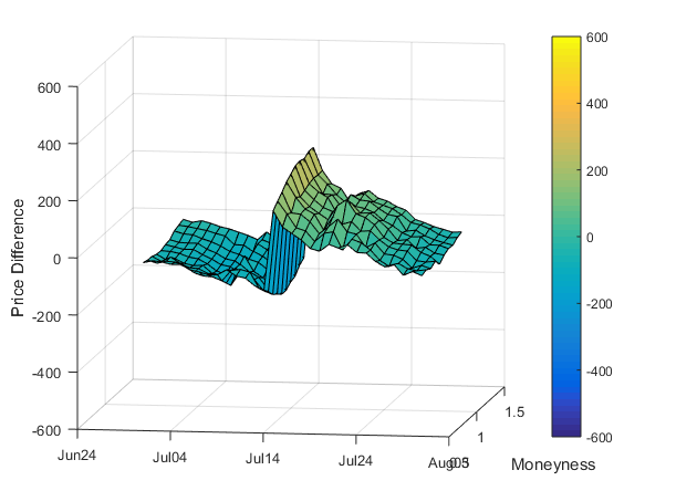
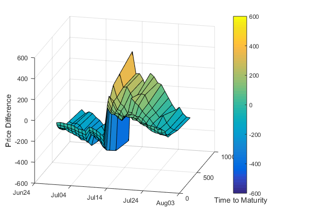
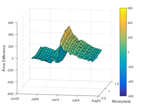
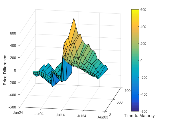
       Figure 1: Call option price differences between the SVCJ and SVJ models, and between the BR and the SVJ models: BTC

       

       

       

       

       Notes: This figure plots the call option price differences between the SVCJ and SVJ models, and call option price differences between the BR and the SVJ models for July 2017. The upper first two plots are the option differences between SVCJ and SVJ, the two plots in the lower panel are the option prices differences between BR and SV. When looking at moneyness, the time to maturity is fixed at 30 days, and when looking at the time to maturity, moneyness is ATM. The colour in the graph represents the price difference level; the brighter the colour, the larger the difference.

   31. On page 32 the paper states :”We can see that the IVs of the BR model agree with the SVCJ model.” When I compare Figures 12 and 13, however, the BR and SVCJ models look completely different. The former implies IVs that are less than one half of the latter. In addition, on a proportional basis, the BR smile is much steeper. So I don’t see much of an agreement. What am I missing?
       

       We thank the AE for the comments. The reason they look different is that we use the realized variance for starting value when estimating the BR options. We use the unconditional sample variance as a starting value when estimating the SVCJ. Now we have used similar initial values for SVCJ and BR, see Figure 9 and 10 on page 26 and page 27 in our manuscript now.
       

       Finally, I would note that the referee offers a number of useful comments as well. I do think that some of the suggestions are a little ambitious, however, especially point #3, in which the referee suggests computing option prices under parameter uncertainty. I like the idea, but maybe itâs better for another paper
       

       We agree with the AE and our revision has tightly followed the AE’s suggestions.
       

3. Referee 1

   The paper provides a time-series analysis of the historical Bitcoin and CRIX (Cryptocurrency Index) price levels. After comparing several econo-metric models, the authors argue that both the SVCJ model and the model based on Bandi and Reno(2016) satisfactorily capture the main features of the dynamics of Bitcoin prices. The authors also apply these models to calculate hypothetical European option prices for Bitcoin and CRIX.

   Considering the fast growth of the cryptocurrency markets, we think this is a timely research that may potentially provide a theoretical foundation for the future development of derivative markets on these new currencies. The following are my comments.

   1. A finding emphasized in the paper is that Bitcoin price displays an ”inverse leverage effect” in the sense that the correlation between the diffusive innovations of the return process and those of the volatility process is positive, which contradicts the findings from equity index re- turns. The leverage effect contributes to the negative skewness observed in equity index returns, which in turn contributes to the volatility smirk in equity index options. In particular, negative skewness causes the implied volatility of OTM puts to be higher than that of ITM puts. Surprisingly, despite the inverse leverage effect, the hypothetical Bitcoin option prices also show a left smirk, just as in stock index options. Intuitively, if volatility rises as the underlying price rises, I would expect a positive skewness in returns and hence an IV smirk that is higher. On the right hand side. Of course, my argument can be overturned by other channels in the models. But I think some explanation should be presented in the paper. I wonder if the direction of the smirk shown in the paper is specific to the date picked to calculate it. I suggest three exercises that can be easily done by the authors. First, report unconditional moments of Bitcoin returns. Second, calculate the IV surfaces for a few randomly selected days in addition to the date already used and look at the direction of the smirk. Third, report the model-implied conditional moments of Bitcoin returns at those selected trading days and examine the relationship between the moments and shapes of the IV surfaces.
      

      We thank referee for the suggestions. The randomly chosen month is July 2019. We have done the procedure as the referee suggested and done a randomly selected day, and we find that the shape of the IVs in the similar shapes we have obtained in the paper.
      

   2. Several places in the paper, the authors argue that the SVCJ model is the best among the affine models considered. I feel that these claims are not always well explained. In the second-to-last paragraph on Page 18, it states ”it is apparent that the SVCJ model is the preferred choice”. But this is not that apparent to me from the QQ plot as SVCJ and SVJ look very similar. Also, Figure 7 is used to assert the superiority of the SVCJ model, but it is unclear to me in what way this figure serves that purpose. The figure demonstrates simulated return distributions based on the three models and shows that SVCJ produces the smallest range for 2.5% to 97.5% percentiles. But how does this speak to the quality of model fitting? In addition, these simulations require the initial level of volatility. What is the value used here? How does that value affect the patterns?
      

      Thank the referee for the suggestions. We agree with the referee that the QQ plot for SVJ and SVCJ look similar. These two models do perform much better than the SV. However, the MSE shows that the SVCJ model reduces to 0.735 compared with the MSE of the SVJ model of 0.757, see Table 1 on Page 12. (We notice that we mixed the QQ plot of the SVCJ and SVJ models. We apologize for the confusion, and we have corrected it in the revised version), see Figure 4 on Page 15. For Figure 7 in the old version of our paper, we use the unconditional variance value as an initial for the simulation. However, we agree with the referee that the figure can hardly serve as a purpose to show the quality of the model fitting. We have taken this figure away from the paper.
      

   3. A major concern of applying a sophisticated model to Bitcoin prices is the lack of a reasonably long history and the resulting errors in parameter estimates. Since the authors adopt the Bayesian framework, they are in a good position to provide valuable discussions regarding the implications of parameter uncertainty. In pricing the options, the authors use the point estimates of the parameters while the posterior distributions suggest large uncertainty in those estimates. If market participants also face the same parameter uncertainty, then I would argue that the current approach in the paper underestimates options prices. It should be easy to investigate this issue by utilizing the empirical posterior distributions of the parameters. Specifically, in CMC, rst draw the parameters from the posterior distributions and then proceed to 2 simulate the Bitcoin prices and calculate option prices. The differences between the option prices calculated this way and those presented in the paper would reflect the effect of parameter uncertainty.
      

      We the referee for the suggestions, however, we agree with AE, that these suggestions might be too ambitious to the current paper, we leave this to be a future research issue.
      

   4. If data are available, I suggest that the authors estimate the SV, SVJ, SVCJ, and BR models using Bitcoin prices updated to fairly recent date and see whether the posterior distributions are stable.
      

      We thank referee for the suggestions. We have tried estimating the models with fairly recent data, and the parameters are similar and the parameters significance level remains the same.
      

   5. In the last five lines on Page 31, the authors state that ”It is interesting to note that all three models have a one-side volatility skew, implying that ITM options prices are higher than the OTM options.” This seems like a strange statement since ITM options are more expensive than OTM options even in the Black-Schole model.
      

      Thanks for referee. We have revised the sentence to make as a normal discovery, see the last paragraph on page 24.
      

   6. The first sentence of the second paragraph on Page 17 has a typo. The first SV should be SVCJ.
      

      Thanks. We have corrected the typo, see the first line of the second paragraph on page 12.