Differentiable Scattering Matrix for Optimization of Photonic Structures

Abstract

The scattering matrix, which quantifies the optical reflection and transmission of a photonic structure, is pivotal for understanding the performance of the structure. In many photonic design tasks, it is also desired to know how the structure’s optical performance changes with respect to design parameters, that is, the scattering matrix’s derivatives (or gradient). Here we address this need. We present a new algorithm for computing scattering matrix derivatives accurately and robustly. In particular, we focus on the computation in semi-analytical methods (such as rigorous coupled-wave analysis). To compute the scattering matrix of a structure, these methods must solve an eigen-decomposition problem. However, when it comes to computing scattering matrix derivatives, differentiating the eigen-decomposition poses significant numerical difficulties. We show that the differentiation of the eigen-decomposition problem can be completely sidestepped, and thereby propose a robust algorithm. To demonstrate its efficacy, we use our algorithm to optimize metasurface structures and reach various optical design goals.

1 introduction

The scattering matrix is a fundamental concept in many fields. It relates the input state and the output state of a physical system undergoing a scattering process. Particularly revealing in optics, the scattering matrix has been widely used for analyzing photonic structures such as waveguides [19, 9, 18] and metasurface units [16, 43, 8]. Once the scattering matrix of a photonic structure is known, the structure’s optical performance (e.g., mode conversion efficiency and phase shift) can be directly obtained.

Because of its vital importance, many numerical methods have been developed to compute the scattering matrix of a photonic structure. Among them, a popular class is the semi-analytical methods, such as the method of lines [28] and rigorous coupled-wave analysis (RCWA) [24]. These methods exploit the fact that many photonic structures in practice (such as waveguides and metasurface units) have a piecewise constant cross-sectional shape along the transmission direction (denoted as $z$-direction). Thus, to solve Maxwell’s equations, they only need to discretize the 2D cross-sectional region, reducing Maxwell’s equations into a set of continuous differential equations along $z$-direction, whose solution can be expressed through an eigenvalue analysis. Thanks to the semi-discretization, these methods often enable faster computation in comparison to full discretization methods (such as finite-element- and finite-volume-based methods). Indeed, methods like RCWA have been widely used in designing various photonic structures, such as metasurfaces [3, 16, 4, 11], metagratings [13, 1], holograms [43, 44], polarimeters [5], solar cells [40], radiative cooling structures [30], color structures [34], photonic crystals[41], and waveguides [19, 9].

In this work, we extend the semi-analytical methods to obtain the higher-order information of scattering matrices, namely the scattering matrix’s derivatives (or gradient). Provided a photonic structure specified by certain design parameters, we aim to compute not only its scattering matrix but its derivatives with respect to the design parameters.

The scattering matrix derivatives depict the changes of the structure’s optical behaviors as its design parameters vary. This higher-order information, if robustly and efficiently computed, finds many applications in photonic design. Most notable is the optimization of photonic structures. The derivatives provide guidance on how we can adjust the parameters (e.g., through the gradient descent algorithm [31]) to improve the structure’s optical performance [20] or to find a design robust to fabrication error [2, 39, 45].

Unfortunately, the computation of scattering matrix derivatives is nontrivial. The difficulty is rooted in the fact that the permissible optical modes in a photonic structure are eigenfunctions of a linear (Hermitian) operator determined by Maxwell’s equations [15]. Thus, to compute the scattering matrix, semi-analytical methods must solve an eigen-decomposition problem: its eigenvalues describe the propagation constants (or effective indices) of the modes and its eigenvectors indicate propagating modal patterns. Differentiating the scattering matrix, by chain rule, requires the derivatives of eigenvalues and eigenvectors. It is the need of eigenvector derivatives that renders the scattering matrix differentiation ill-posed: when there exist repeated eigenvalues, the corresponding eigenvectors are not uniquely defined. As the parameter changes, the numerical results of the eigenvectors may change discontinuously, and their derivatives become undefined (see more discussion in Section 3).

Not merely does this issue exist as a corner case; many photonic structures in practice have geometric and material symmetries, from which repeated eigenvalues and thus ill-defined eigenvector derivatives emerge (see Fig. 2). Consequently, one must carefully choose eigenvectors such that they vary smoothly with respect to the design parameters. This choice, albeit attainable, demands complex and expensive computational effort [38].

In this paper, we question the necessity of eigenvector derivatives for differentiating scattering matrices. We show that while eigen-decompositions are needed for computing a photonic structure’s scattering matrix, eigenvector derivatives can be fully sidestepped for differentiating the scattering matrix. Based on our new derivation, we present a fast and robust algorithm that, without resorting to eigenvector derivatives, computes the scattering matrix derivatives with respect to any design parameters.

Our method is designed for scattering matrices in general, independent from any specific basis representation; nor is it bound to any particular geometric parameterization. To demonstrate the use of our method, we apply the scattering matrix derivatives for optimizing the design of metasurface units. We can choose different design parameterizations and use gradient-based optimization to reach various light transmission goals. We also propose a general parameterization of the meta-unit’s cross-sectional shape that can be optimized using our method.

2 Background: Scattering Matrix

We start by briefly reviewing the classic notion of scattering matrix in computational photonics, to pave the way toward its differentiation.

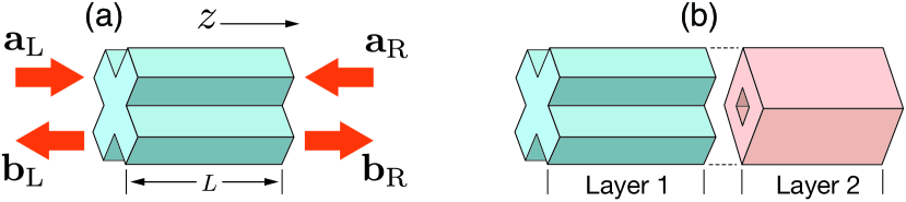
Figure 1: (a) In a photonic structure, light may be incident from both sides and get scattered out. The relationship of incident and scattered light is characterized by the scattering matrix. (b) A complex structure can be decomposed into individual layers. Each layer is characterized by its scattering matrix, and these scattering matrices are then combined (using the Redheffer star product [29]) to form the scattering matrix of the entire structure.

To numerically analyze a photonic structure (such as a waveguide), the structure is often discretized along the wave propagation direction (i.e., $z$-direction) into a series of layers each with a uniform cross-sectional material distribution (Fig. 1-b). Consider optical waves of a specific frequency. Their propagation in each layer is characterized by a scattering matrix $\mathbf{S}$, which relates waves incident on the layer from left and right sides (Fig. 1-a) to the waves scattered out in either direction.

Concretely, let $\mathbf{a}_{\text{L}}$ and $\mathbf{a}_{\text{R}}$ denote vectors describing incident waves on the layer from left and right sides, respectively. Here $\mathbf{a}_{\text{L}}$ and $\mathbf{a}_{\text{R}}$ stack coefficients that represent the waves under a chosen basis, whose construction will be outlined shortly. Under the same basis, we use $\mathbf{b}_{\text{L}}$ and $\mathbf{b}_{\text{R}}$ to denote the scattered waves in left and right directions. With these notations, the incident and scattered waves are related through

$$\begin{bmatrix}\mathbf{b}_{\text{L}}\\ \mathbf{b}_{\text{R}}\end{bmatrix}=\mathbf{S}\begin{bmatrix}\mathbf{a}_{\text{L}}\\ \mathbf{a}_{\text{R}}\end{bmatrix},\text{ where }\mathbf{S}\coloneqq\begin{bmatrix}\mathbf{R}_{\text{L}}&\mathbf{T}_{\text{RL}}\\ \mathbf{T}_{\text{LR}}&\mathbf{R}_{\text{R}}\end{bmatrix}.$$ (1)

Here $\mathbf{S}$ is decomposed into four submatrices: $\mathbf{R}_{\text{L}}$ and $\mathbf{R}_{\text{R}}$ indicate how the incident wave from left or right direction is reflected by the layer, while $\mathbf{T}_{\text{RL}}$ and $\mathbf{T}_{\text{LR}}$ describe how the incident wave (from either direction) transmits through the layer.

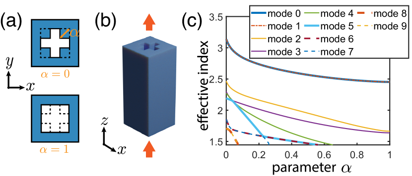
Figure 2: Repetition from symmetry. Consider a meta-atom structure (b) whose cross-sectional shape (a) is parameterized by $\alpha$, which controls the size of the cross-shaped hollow region. The shape symmetry causes the structure’s propagating modes to have repeated effective indices (c), as also indicated by the repeated eigenvalues when one solves (2). As $\alpha$ varies, mode 0 and mode 1 always have the same effective index, meaning that their first-order and higher-order derivatives of the corresponding eigenvalues with respect to $\alpha$ are always the same, and thus their eigenvector derivatives are not mathematically well-defined. The same issue occurs in other modes when $\alpha$ becomes small and more propagating modes appear (e.g., see mode 5 and mode 6 when $\alpha$ is within $\sim[0.3,0.5]$).

The computation of scattering matrix starts with a semi-discretization of the frequency-domain Maxwell’s equations of a photonic layer, namely,

$$-jk_{0}\frac{\partial}{\partial z}\mathbf{e}=\mathbf{P}\mathbf{h}\;\textrm{ and }\;-jk_{0}\frac{\partial}{\partial z}\mathbf{h}=\mathbf{Q}\mathbf{e},$$ (2)

where $k_{0}$ is the free-space wave number, and the vectors $\mathbf{e}$ and $\mathbf{h}$ describe the electric and magnetic fields of the photonic structure under a chosen basis—for example, RCWA uses the 2D Fourier basis on the cross-section of the wave propagation direction. The matrices $\mathbf{P}$ and $\mathbf{Q}$ encode the cross-sectional distributions of material permeability and permittivity.

The semi-discretization (2) is a common form in many numerical analysis methods for photonic structures (such as the method of line [28] and RCWA [24]). The difference across those methods only lies in the specific ways of constructing $\mathbf{P}$ and $\mathbf{Q}$ (e.g., see Supplement 1 for their construction in RCWA).

Once $\mathbf{P}$ and $\mathbf{Q}$ are determined, the scattering matrix $\mathbf{S}$ can be constructed. A key step of this construction is to solve an eigenvalue problem, $(\mathbf{P}\mathbf{Q})\mathbf{W}=\mathbf{W}\bm{\Gamma}$, to obtain eigenvectors $\mathbf{W}$ and the diagonal eigenvalue matrix $\bm{\Gamma}$. As we will discuss in Section 3, it is this eigenproblem that renders the differentiation of the scattering matrix ill-posed. To understand the challenges and how we overcome them, we first present the recipe of computing $\mathbf{S}$ from $\mathbf{W}$ and $\bm{\Gamma}$, as follows.

Let $\bm{\Omega}\coloneqq(\mathbf{P}\mathbf{Q})^{\frac{1}{2}}$. Then, its eigenvalue matrix is $\bm{\Lambda}=\bm{\Gamma}^{\frac{1}{2}}$. As derived in [32], the formulas of computing the scattering matrix $\mathbf{S}$ defined in (1) are

$$\mathbf{R}_{\textrm{L}}=\mathbf{R}_{\textrm{R}} =\left(\mathbf{A}-\mathbf{X}\mathbf{B}\mathbf{A}^{-1}\mathbf{X}\mathbf{B}\right)^{-1}\left(\mathbf{X}\mathbf{B}\mathbf{A}^{-1}\mathbf{X}\mathbf{A}-\mathbf{B}\right),$$ (3a)

$$\mathbf{T}_{\text{LR}}=\mathbf{T}_{\text{RL}} =\left(\mathbf{A}-\mathbf{X}\mathbf{B}\mathbf{A}^{-1}\mathbf{X}\mathbf{B}\right)^{-1}\mathbf{X}\left(\mathbf{A}-\mathbf{B}\mathbf{A}^{-1}\mathbf{B}\right),$$ (3b)

where the matrices $\mathbf{X}$, $\mathbf{A}$, and $\mathbf{B}$ have the following forms:

$$\mathbf{X} =e^{j\bm{\Lambda}\frac{L}{k_{0}}},$$ (4a)

$$\mathbf{A} =\mathbf{W}^{-1}\mathbf{W}_{0}+\mathbf{V}^{-1}\mathbf{V}_{0},\;\text{ and }\mathbf{B}=\mathbf{W}^{-1}\mathbf{W}_{0}-\mathbf{V}^{-1}\mathbf{V}_{0}.$$ (4b)

Here we use $L$ to denote the layer thickness (Fig. 1), and the matrix $\mathbf{V}$ is related to $\mathbf{W}$ through $\mathbf{V}=\mathbf{Q}\mathbf{W}\bm{\Lambda}^{-1}$. $\mathbf{W}$ and $\mathbf{V}$ together form a basis of electric and magnetic components for the optical waves in the layer. Similarly, $\mathbf{W}_{0}$ and $\mathbf{V}_{0}$ form a basis for free space propagation, independent from the photonic structure. They are constant values for computing the derivatives of $\mathbf{S}$. The vectors, $\mathbf{a}_{\text{L}}$, $\mathbf{a}_{\text{R}}$ $\mathbf{b}_{\text{L}}$, and $\mathbf{b}_{\text{R}}$, in (1) are coefficients under this free-space basis to describe incident and scattered waves.

Once the scattering matrices of individual layers are computed, they are combined using the Redheffer star product [29] into the total scattering matrix, one that indicates the optical response of the entire photonic structure.

Remark. The formulas in Eqs. (3) and (4) assume that the current photonic layer is sandwiched by two free-space layers. This assumption is by no means a limitation. In an arbitrary photonic structure, the layers can be treated as if they are interleaved with free-space layers—each of which has a zero thickness.

3 Differentiable Scattering Matrix

The geometry or material distribution of photonic structure is specified by its structural (design) parameters (e.g., see Fig. 2). These parameters determine the structure’s permittivity and permeability distributions described by $\mathbf{P}$ and $\mathbf{Q}$ in (2). Thus, one can compute their derivatives, $\mathbf{P}^{\prime}$ and $\mathbf{Q}^{\prime}$, with respect to an arbitrary parameter. Given $\mathbf{P}^{\prime}$ and $\mathbf{Q}^{\prime}$, we now address the question of how to compute the scattering matrix derivative $\mathbf{S}^{\prime}$ with respect to the same parameter.

3.1 Challenges in Scattering Matrix Differentiation

The construction of scattering matrix $\mathbf{S}$ needs to solve an eigenvalue problem $(\mathbf{P}\mathbf{Q})\mathbf{W}=\mathbf{W}\bm{\Gamma}$, as the eigenvalues $\bm{\Gamma}$ and eigenvectors $\mathbf{W}$ appear in Eqs. (3) and (4) for computing $\mathbf{S}$. Thus, for the differentiation of $\mathbf{S}$, it seems also needed to compute the derivatives of the eigenvalues $\bm{\Gamma}$ and eigenvectors $\mathbf{W}$.

Unfortunately, the derivatives of eigenvectors in many cases are ill-defined. Most notable is when there exist repeated eigenvalues. Repeated eigenvalues are not uncommon: many photonic devices have certain structural symmetries, from which eigenvalue repetition naturally emerges (see Fig. 2). For those repeated eigenvalues, their eigenvectors (up to a scale) are not uniquely determined; any set of linearly independent vectors that span the same subspace are valid eigenvectors. Because of the ambiguity, as the structural parameter changes, those eigenvectors may change discontinuously (see an examples in Supplement 1), and thus their derivatives may not be well-defined.

As a result, one must carefully choose eigenvectors in the subspace of repeated eigenvalues such that the eigenvectors change continuously with respect to the structural parameter. This choice, however, is computationally expensive. As derived in [38], to ensure well-defined eigenvector derivatives, one must compute higher-order derivatives of the eigenvalues and the matrix $\mathbf{P}\mathbf{Q}$: if the repeated eigenvalues have repeated derivatives up to the $n$-th order (see Fig. 2), then derivatives up to the $(n+1)$-th order of both eigenvalues and the matrix $\mathbf{P}\mathbf{Q}$ must be computed to determine first-order eigenvector derivatives.

3.2 Differentiation without Resort to Eigenvector Derivatives

We now present a new algorithm for computing the scattering matrix derivative $\mathbf{S}^{\prime}$. Even in the presence of repeated eigenvalues and their derivatives, our method requires only the first-order derivatives of the matrices $\mathbf{P}$ and $\mathbf{Q}$, completely sidestepping the differentiation of eigenvalues and eigenvectors. In comparison to the way that takes eigenvalue derivatives (as described above), our method is more robust and efficient.

First, we rewrite the commonly used expressions of scattering matrix components, shown in (3), in new forms,

$$\mathbf{R}_{\textrm{L}}=\mathbf{R}_{\textrm{R}} =\left(\mathbf{I}-\mathbf{D}_{1}^{2}\right)^{-1}\left(\mathbf{D}_{1}\mathbf{D}_{2}-\mathbf{D}_{3}\right),$$ (5a)

$$\mathbf{T}_{\text{LR}}=\mathbf{T}_{\text{RL}} =\left(\mathbf{I}-\mathbf{D}_{1}^{2}\right)^{-1}\left(\mathbf{D}_{2}-\mathbf{D}_{1}\mathbf{D}_{3}\right),$$ (5b)

where $\mathbf{D}_{1}$, $\mathbf{D}_{2}$, and $\mathbf{D}_{3}$ denote the following matrix multiplications, respectively:

$$\mathbf{D}_{1} \coloneqq\mathbf{A}^{-1}\mathbf{X}\mathbf{B}=\left(\mathbf{W}_{0}+\mathbf{T}\mathbf{V}_{0}\right)^{-1}\mathbf{W}\mathbf{X}\mathbf{W}^{-1}\left(\mathbf{W}_{0}-\mathbf{T}\mathbf{V}_{0}\right),$$ (6a)

$$\mathbf{D}_{2} \coloneqq\mathbf{A}^{-1}\mathbf{X}\mathbf{A}=\left(\mathbf{W}_{0}+\mathbf{T}\mathbf{V}_{0}\right)^{-1}\mathbf{W}\mathbf{X}\mathbf{W}^{-1}\left(\mathbf{W}_{0}+\mathbf{T}\mathbf{V}_{0}\right),$$ (6b)

$$\mathbf{D}_{3} \coloneqq\mathbf{A}^{-1}\mathbf{B}=\left(\mathbf{W}_{0}+\mathbf{T}\mathbf{V}_{0}\right)^{-1}\left(\mathbf{W}_{0}-\mathbf{T}\mathbf{V}_{0}\right).$$ (6c)

The derivation of these new expressions (5) and (6) are provided in Supplement 1. In Eqs. (6), the equalities are reached by applying (4) and using $\mathbf{T}$ that denotes $\mathbf{T}\coloneqq\bm{\Omega}\mathbf{Q}^{-1}$.

The expressions in (5) present a new route for computing scattering matrix derivative. They indicate that the scattering matrix $\mathbf{S}$ is determined by the three matrices, $\mathbf{D}_{1}$, $\mathbf{D}_{2}$, and $\mathbf{D}_{3}$. As a result, to compute its derivative $\mathbf{S}^{\prime}$ using the chain rule, we need to compute the derivatives of $\mathbf{D}_{1}$, $\mathbf{D}_{2}$, and $\mathbf{D}_{3}$ with respect to the structural parameter.

In Eqs. (6), both $\mathbf{W}_{0}$ and $\mathbf{V}_{0}$ (introduced in (4)) are constant matrices. Thus, the derivatives of $\mathbf{D}_{1}$, $\mathbf{D}_{2}$, and $\mathbf{D}_{3}$ only depend on the derivatives of two other matrices in Eqs. (6), namely $\mathbf{T}$ and $\mathbf{W}\mathbf{X}\mathbf{W}^{-1}$. We now describe how to compute the derivatives of the two matrices, respectively.

Derivative of $\mathbf{T}$.

The matrix $\mathbf{T}\coloneqq\bm{\Omega}\mathbf{Q}^{-1}$ is related to $\mathbf{Q}$ and $\bm{\Omega}\coloneqq\left(\mathbf{P}\mathbf{Q}\right)^{{1}/{2}}$ but not the eigenvalues and eigenvectors. Its derivative can be expressed as

$$\mathbf{T}^{\prime}=\bm{\Omega}^{\prime}\mathbf{Q}^{-1}+\bm{\Omega}\left(\mathbf{Q}^{-1}\right)^{\prime}=\bm{\Omega}^{\prime}\mathbf{Q}^{-1}-\bm{\Omega}\mathbf{Q}^{-1}\mathbf{Q}^{\prime}\mathbf{Q}^{-1},$$ (7)

where $\mathbf{Q}$ depends on the material permittivity distributions of the photonic structure, and therefore its derivative $\mathbf{Q}^{\prime}$ with respect to a design parameter can be directly computed (see examples in Section 4). The way of computing $\bm{\Omega}^{\prime}$ can be derived by taking the derivatives on both sides of the relation $\bm{\Omega}^{2}=\mathbf{P}\mathbf{Q}$, which yields

$$\bm{\Omega}^{\prime}\bm{\Omega}+\bm{\Omega}\bm{\Omega}^{\prime}=\mathbf{P}^{\prime}\mathbf{Q}+\mathbf{P}\mathbf{Q}^{\prime}.$$ (8)

Given $\mathbf{P}^{\prime}$ and $\mathbf{Q}^{\prime}$, the right-hand side of this equation can be directly computed. To compute $\bm{\Omega}^{\prime}$, we rewrite the left-hand side by denoting $\bm{\Omega}^{\prime}$ as $\bm{\Omega}^{\prime}=\mathbf{W}\mathbf{Y}\mathbf{W}^{-1}$ for some unknown $\mathbf{Y}$, where $\mathbf{W}$ is the eigenvector matrix of $\mathbf{P}\mathbf{Q}$. Using the fact that $\bm{\Omega}=(\mathbf{P}\mathbf{Q})^{1/2}=\mathbf{W}\bm{\Lambda}\mathbf{W}^{-1}$, we obtain a simplified form of (8):

$$\mathbf{Y}\bm{\Lambda}+\bm{\Lambda}\mathbf{Y}=\mathbf{W}^{-1}(\mathbf{P}^{\prime}\mathbf{Q}+\mathbf{P}\mathbf{Q}^{\prime})\mathbf{W}.$$ (9)

From (9), $\mathbf{Y}$ can be easily solved by noticing that $\bm{\Lambda}$ is a diagonal matrix, and therefore (9) can be written element-wise as $(\lambda_{i}+\lambda_{j})\mathbf{Y}_{ij}=\mathbf{C}_{ij}$, where $\lambda_{i}$ is the $i$-th eigenvalue in $\bm{\Lambda}$, and $\mathbf{C}$ denote the matrix on the right-hand side of (9). In other words, the elements of $\mathbf{Y}$ can be obtained by solving $n^{2}$ 1D linear equations in parallel. Once $\mathbf{Y}$ is obtained, $\bm{\Omega}^{\prime}$ is computed using $\bm{\Omega}^{\prime}=\mathbf{W}\mathbf{Y}\mathbf{W}^{-1}$.

We note that while this process of computing $\bm{\Omega}^{\prime}$ requires the eigenvectors $\mathbf{W}$ and eigenvalues $\bm{\Lambda}$, they are also needed for computing the scattering matrix in the first place. Our solving process does not require the derivatives of eigenvectors. Therefore, it introduces no additional effort in terms of eigen-decomposition.

Derivative of $\mathbf{W}\mathbf{X}\mathbf{W}^{-1}$.

In the first glance, the derivative of $\mathbf{W}\mathbf{X}\mathbf{W}^{-1}$ depends on the eigenvectors $\mathbf{W}$. However, from the definition of $\mathbf{X}$ in (4a), we notice that $\mathbf{W}\mathbf{X}\mathbf{W}^{-1}=e^{j\bm{\Omega}{L}/{k_{0}}}$, which suggests an alternative approach: take the derivative of the matrix exponential $e^{j\bm{\Omega}{L}/{k_{0}}}$ with respect to $\bm{\Omega}$.

A common approach of computing the matrix exponential $e^{j\bm{\Omega}{L}/{k_{0}}}$ is through the eigen-decomposition of $\bm{\Omega}$ followed by the exponential of the resulting eigenvalues. If we take this approach, the derivative computation must involve the derivatives of eigenvectors, which might not be well-defined. Another approach, used by Feynman [12] and others [17, 7, 35], expresses the derivative of a matrix exponential using an integral that in itself involves matrix exponentials. Yet, numerically evaluating the matrix exponentials and the integral are expensive.

Instead, our proposed method for computing the derivative is based on the following proposition originally proved in [25].

Proposition 1.

Consider an $n\times n$ matrix $\bm{\Omega}$ and its derivative $\bm{\Omega}^{\prime}$ with respect to an arbitrary parameter. If

$$\mathbf{G}=\begin{bmatrix}\bm{\Omega}&\bm{\Omega}^{\prime}\\ \mathbf{0}&\bm{\Omega}\end{bmatrix},\;\textrm{then }e^{j\mathbf{G}{L}/{k_{0}}}=\begin{bmatrix}e^{j\bm{\Omega}{L}/{k_{0}}}&\left(e^{j\bm{\Omega}{L}/{k_{0}}}\right)^{\prime}\\ \mathbf{0}&e^{j\bm{\Omega}{L}/{k_{0}}}\end{bmatrix},$$ (10)

where the top-right $n\times n$ block matrix in $e^{j\mathbf{G}{L}/{k_{0}}}$ is the derivative of the matrix exponential $e^{j\bm{\Omega}{L}/{k_{0}}}$.

In our problem, $\bm{\Omega}^{\prime}$ is computed as described above (by solving (9)), and the common way of computing $e^{j\mathbf{G}{L}/{k_{0}}}$ is by taking the eigen-decomposition of $\mathbf{G}$, which is again what we wish to avoid. We therefore take a different approach, the scaling and squaring method [14], to compute $e^{j\mathbf{G}{L}/{k_{0}}}$—without the need of eigen-decomposition.

The scaling and squaring method exploits the relation $e^{\mathbf{A}}=\left(e^{\mathbf{A}/\sigma}\right)^{\sigma}$ for any $n\times n$ matrix $\mathbf{A}$. In practice, $\sigma$ is chosen to be $\sigma=2^{s}$ for some non-negative integer $s$. The idea is to have the norm of $\mathbf{A}/\sigma$ sufficiently small such that $e^{\mathbf{A}/\sigma}$ can be well approximated by a Padé approximant near the origin. The Padé approximant is a rational polynomial of $\mathbf{A}$. Its evaluation requires only matrix multiplications and inverse, but no eigen-decomposition. The scaling and squaring method is robust and accurate, and has been used in many numerical tools (such as MATLAB’s expm function).

When applying this method, we further exploit the specific structure of $\mathbf{G}$ (i.e., its bottom-left block matrix vanishes, and its two diagonal block matrices are identical) to tailor the method for improving computational performance. Supplement 1 presents our detailed derivations and computational steps.

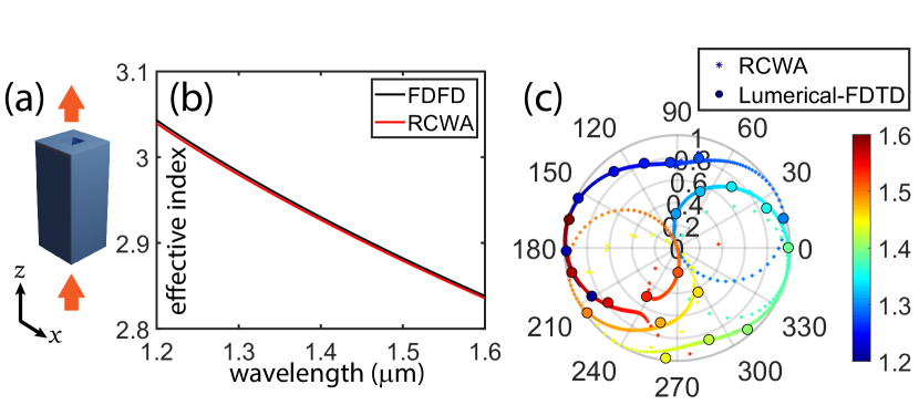
Figure 3: Accuracy comparison. (a) We use our method and FDTD (Lumerical [36]) to analyze a 3D meta-atom. The width of the pillar and its square hole are $0.6\mu\text{m}$ and $0.2\mu\text{m}$, respectively, and it has a height of 1.4 $\mu\text{m}$. We use the periodic boundary condition, with the period of $0.66\mu\text{m}$. (b) We scan the (x-polarized) wavelength and plot the effective indices of the fundamental mode evaluated by FDFD and our method. (c) For each wavelength (color mapped here), we compute the far-field amplitudes and phases changes, and compare our results to FDTD.

4 Results

This section presents our numerical results. First, we validate our algorithm for computing scattering matrix derivatives. Next, to demonstrate the use of scattering matrix derivatives in photonics, we optimize the geometry of photonic metasurface units (also called meta-atoms).

Meta-atoms are the building blocks of a metasurface, often designed based on physical intuitions and manually crafted libraries [42, 27, 26]. More recently, inverse design methods of meta-atom structures have also been explored—e.g., through finite-difference-based gradient descent [6], adjoint-based level-set method [23], and topological optimization [33, 22].

Due to fabrication constraints, meta-atoms often have constant cross-sectional shapes along one direction (i.e., $z$-direction, as shown in Fig. 3-a). Thus, the semi-analytical methods (such as RCWA) are particularly efficient for simulating meta-atoms, thanks to their ability of not discretizing along $z$-direction [24]. Our method, for the first time, enables the semi-analytical methods to also compute scattering matrix derivatives with respect to design parameters. Here, in the framework of RCWA, we demonstrate automatic discovery of meta-atom structures that reach various amplitude and phase goals.

4.1 Validation

To validate our algorithm, we consider a dielectric meta-atom used in metasurface holography [26, 27]. Its structure is shown in Fig. 3-a. We use Eqs. (5) to compute the scattering matrix, for which the matrices $\mathbf{P}$ and $\mathbf{Q}$ (introduced in (2)) are constructed using RCWA. The scattering matrix allows us to compute light propagation properties of the meta-atom, which are in turn compared to the results from finite difference time domain (FDTD) method implemented in Lumerical [36].

We first scan the light wavelength from $1.2\mu\text{m}$ to $1.6\mu\text{m}$. For each wavelength, we compute, using our scattering matrix and FDFD respectively, the effective index of the fundamental mode propagating in the meta-atom. The results from our method agree with FDFD results (see Fig. 3-b). Furthermore, we consider the far-field light transmission through the meta-atom, and compute the phase shift and amplitude change for each wavelength. Again, the results from our method and FDTD match closely, as shown in Fig. 3-c.

These experiments confirm that our scattering matrix computation is as accurate as FDTD in Lumerical. In terms of computational cost, our method takes about 0.15 seconds for each monochromatic simulation, and a few seconds for the entire $1.2\mu\text{m}$-$1.6\mu\text{m}$ wavelength range, whereas the FDTD simulation takes several minutes.

Next, we validate our derivative computation. We consider again the meta-atom structure shown in Fig. 3-a, and choose the parameter $\alpha$ to be the size of the hollow square. Using our method, we compute the derivative of the structure’s scattering matrix with respect to $\alpha$. Meanwhile, since there is no analytic expression of the scattering matrix derivative, we approximate it using finite difference (FD) estimation, that is,

$$\frac{\partial\mathbf{S}}{\partial\alpha}\approx\frac{\mathbf{S}(\alpha+\Delta\alpha)-\mathbf{S}(\alpha-\Delta\alpha)}{2\Delta\alpha}.$$ (11)

We estimate $\frac{\partial\mathbf{S}}{\partial\alpha}$ using a sweeping range of $\Delta\alpha$ values, and compare them to the derivative resulted from our method.

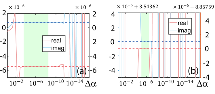
Figure 4: Scattering matrix derivatives. We choose two matrix elements in the scattering matrix, and plot their FD derivatives estimated with different FD sizes ($\Delta\alpha$ in $x$-axis) in (a) and (b), respectively. In each plot, the red and blue solid curves correspond to the real and imaginary parts of the estimated derivative. Meanwhile, the derivatives computed by our method are indicated by the red (real) and blue (imaginary) horizontal dash lines. These plots show that FD estimation is highly sensitive to $\Delta\alpha$. Light green regions indicate valid $\Delta\alpha$ ranges for both matrix elements. The valid $\Delta\alpha$ varies element by element. Thus, in practice, it is hard to choose a proper $\Delta\alpha$ for the entire scattering matrix, whereas our method is always robust.

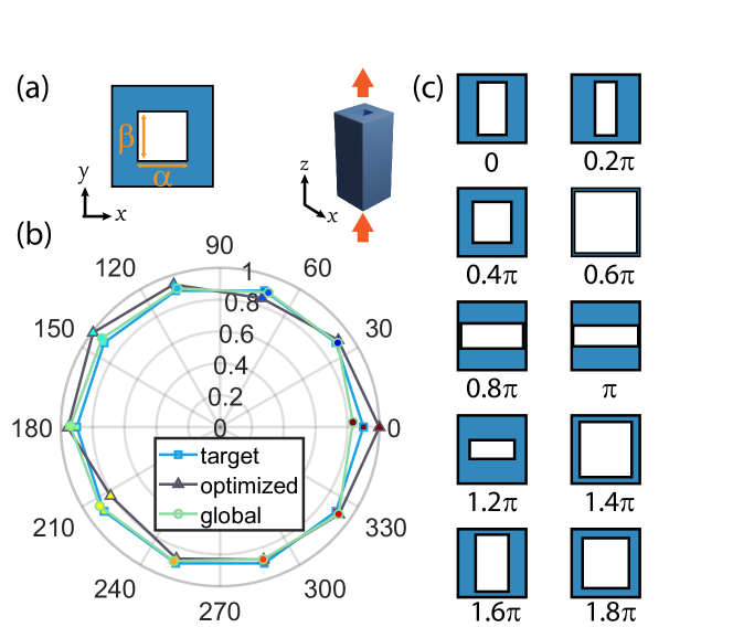
Figure 5: Optimization of (12). (a) We optimize the cross-sectional shape specified by two design parameters $\alpha$ and $\beta$ in order to reach a target transmission amplitude and phase. We examine different targets evenly sampled on a circle on the complex plane (indicated by the square dots in (b)). The optimized amplitudes and phases (indicated by triangular dots) reach closely to the targets. As a reference, we also show the amplitudes and phases (in circular dots) of the designs that globally minimize (12), that is, ones obtained through a slow, exhaustive search of all parameter combinations. While no gradient-based optimization algorithm can guarantee the global minimum of (12), our results approach the targets closely, comparable to what the global minimums can achieve. The resulting cross-sectional shape for each sampled target are shown in (c).

The results are illustrated in Fig. 4. The accuracy of FD approximation largely depends on the choice of $\Delta\alpha$. Only when $\Delta\alpha$ is chosen within a certain range, FD approximation is accurate enough to agree with our derivative results. This agreement confirms the correctness of our method. But for different elements in the scattering matrix, the valid $\Delta\alpha$ range varies (indicated in light green in Fig. 4), suggesting that FD approximation is impractical: it is hard, if not impossible, to choose a proper $\Delta\alpha$ to produce accurate derivative estimations for all elements in the scattering matrix. In contrast, our method is robust for computing the derivatives.

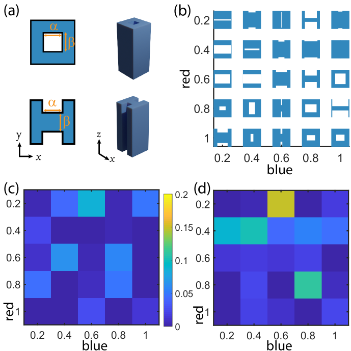
Figure 6: Optimization of (14). (a) We optimize meta-atom structures described by two archetypes, each with two parameters. The goal is to obtain desired amplitude responses at two separate wavelengths (i.e., 1.2$\mu\text{m}$ (blue) and 1.6$\mu\text{m}$ (red)), simultaneously. We sample five amplitudes from 0.2 to 1 for each wavelength, forming 25 different optimization targets. Each target leads to a different cross-sectional design shown in (b). For red light, the discrepancies between achieved amplitudes and the targets are shown in (c), and the same visualization for blue light is shown in (d).

Computational cost.

In addition to the robustness, our method is also faster than the FD method. In the FD method, computing a matrix derivative requires the computation of two scattering matrices $\mathbf{S}(\alpha+\Delta\alpha)$ and $\mathbf{S}(\alpha-\Delta\alpha)$. In contrast, our method, in addition to computing $\mathbf{S}(\alpha)$, only requires a few matrix multiplications and inverses (recall Section 3.3.2). On our workstation computer, the overhead of computing a scattering matrix derivative is about $30\%\sim 40\%$ of the cost for computing the scattering matrix itself.

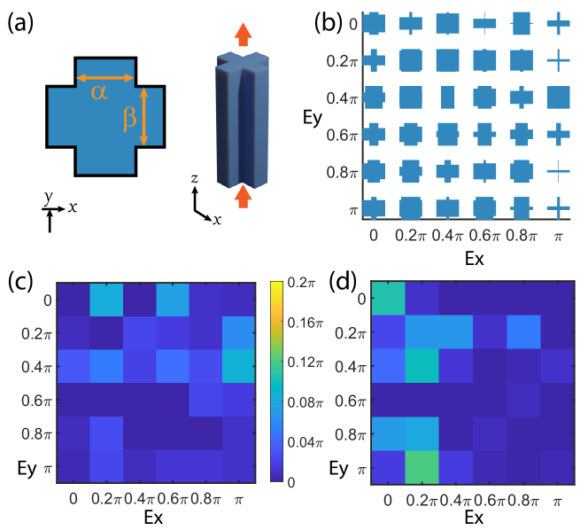
Figure 7: Optimization of (13). (a) We optimize the meta-atom structure described by two parameters. The goal is to achieve certain phase changes for $x$- and $y$-polarized light simultaneously. (b) We sample six target phase changes for $x$- and $y$-polarized light, respectively. Their combination forms 36 different optimization targets. For each target, our optimization produces a cross-sectional shape design. (c) For $x$-polarized incident light, we show the residual (in terms of phase angle difference) between each pair of inversely designed phase change and the target. And similar visualization for $y$-polarized light is shown in (d).

4.2 Use Case: Optimization of Meta-atom Structure

Controlling phase and amplitude of monochromatic light.

First, we optimize meta-atom structures to reach specific transmitted amplitudes and phases for a monochromatic light (at 1.55$\mu\text{m}$ wavelength, $x$-polarized). The cross-sectional shape is shown in Fig. 5-a, determined by two parameters. The objective function for the inverse design is defined as

$$\mathcal{L}={\left|\mathbf{T}_{\text{LR}}(m,m)-t_{m}\right|}^{2},$$ (12)

where $\mathbf{T}_{\text{LR}}$ is the transmission submatrix in the scattering matrix (recall (1)), $m$ is the mode index for the incident and outgoing light in free space, thus $\mathbf{T}_{\text{LR}}(m,m)$ denotes the $m$-th diagonal element of the matrix. Also, $t_{m}$ is a complex constant specifying the target amplitude and phase of the transmission. Here we consider the fundamental mode (the way to choose corresponding $m$ is given in Supplemental 1), which describes the far-field light transmission along the $z$-direction.

To verify the robustness of our method and the enabled optimization, we evenly sample different targets $t_{m}$ on a circle on the complex plane (see Fig. 5-b). For each target, we find meta-atom’s shape parameters by minimizing (12) through a gradient-descent algorithm [31], for which the gradients of (12) with respect to the design parameters are computed using our method. As shown in Fig. 5-b, we are able to automatically discover structures that reach these targets closely.

Controlling phases for both $x-$ and $y-$polarized light.

Next, we optimize meta-atom structures to obtain target responses for $x$- and $y$-polarized light, simultaneously. This type of meta-atoms has been used to construct metasurface holograms [10]. In our example, the light wavelength is 1.3$\mu\text{m}$; the meta-atoms have a fixed height of 2.0$\mu\text{m}$ and a period of 2.5$\mu\text{m}$ along $x$- and $y$-direction. The cross-sectional shape of the meta-atoms are specified by two parameters shown in Fig. 7-a. We determine the parameters by minimizing the following objective function:

$$\mathcal{L}=-\frac{\mathbf{T}_{\text{LR}}(m_{x},m_{x})}{\left|\mathbf{T}_{\text{LR}}(m_{x},m_{x})\right|}t_{x}^{*}-\frac{\mathbf{T}_{\text{LR}}(m_{y},m_{y})}{\left|\mathbf{T}_{\text{LR}}(m_{y},m_{y})\right|}t_{y}^{*},$$ (13)

where the subscript $x$ (and $y$) indicates light polarization; $t_{x}$ (and $t_{y}$) are the target phase changes from $x$-polarized (and $y$-polarized) incident light to the outgoing light with the same polarization (i.e., $t_{x}=\exp(i\phi_{x})$ for some $\phi_{x}$). The first term in (13) measures, for the $x$-polarized light, the cosine difference (through dot product on complex plane) between the $m$-th mode’s phase change and the target phase change, and similarly for the second term. The optimized structures for different $x$- and $y$-polarized phase targets are shown in Fig. 7. In all cases, the residual between the target and the resulting phase change is within 7% of one period ($2\pi$), and in most cases within 1%.

Controlling amplitudes for multiple wavelengths.

We also demonstrate inverse design of meta-atoms for another type of optical response: obtain two target amplitude responses at two separate wavelengths, simultaneously. This type of responses have proven useful for making colored metasurface holograms [26, 27]. Here we consider two archetypes used in [27], each described by two parameters (see Fig. 6-a). The two wavelengths under consideration are 1.2$\mu\text{m}$ (labeled as blue) and 1.6$\mu\text{m}$ (red), and the objective function is defined as

$$\mathcal{L}=\left[\left|\mathbf{T}_{\text{LR},1}(m,m)\right|^{2}-A^{2}_{1}\right]^{2}+\left[\left|\mathbf{T}_{\text{LR},2}(m,m)\right|^{2}-A^{2}_{2}\right]^{2}.$$ (14)

Here the subscript “1” and “2” indicate the blue (1.2$\mu\text{m}$) and red (1.6$\mu\text{m}$) wavelength, respectively. The first term accounts for the blue wavelength: $\mathbf{T}_{\text{LR},1}$ is the transmission submatrix of the scattering matrix and $A_{1}$ is the desired amplitude. Similar is the second term. More terms can be added in (14) to incorporate more than two wavelengths.

For each archetype, we find its parameter values via a gradient-descent algorithm that minimizes (14), and choose between the two archetypes one that produces a smaller objective value. The optimized structures and their performances are shown in Fig. 6. For almost all the experiments (each with a different amplitude target), the resulting amplitudes by the inversely designed meta-atoms match closely to their targets.

General cross-sectional shape design.

Lastly, we introduce a new way to inverse design the meta-atom’s cross-sectional shape under a general representation. We use the star-convex polygon [37] to represent the cross-sectional shape. Such a shape can be discretized by sampling $N$ points on its boundary so that the polar angles of these points are evenly distributed over $[0,2\pi]$. In other words, the $(k+1)$-th point has the coordinate $p_{k}\left[\cos{\left(2k\pi/N\right)},-\sin{\left(2k\pi/N\right)}\right]$, where $p_{k}$ is a non-negative value (see Fig. 8-a), and the shape is specified by $N$ parameters $p_{1},\ldots,p_{N}$. A large $N$ offers many degrees of freedom to represent a complex shape, but meanwhile renders exhaustive search through the entire parameter space too expensive—one must rely on numerical optimization methods to determine the parameter values.

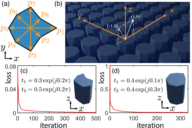
Figure 8: Inverse design of star-convex meta-atoms. (a) The star-convex polygon is used to represent the cross-section of a meta-atom, defined by many control variables ($p_{1}$…$p_{8}$ in this case). As an example, we inverse design the shape for reaching target amplitudes and phases in two scattering directions (i.e., corresponding to diffraction orders (-1,0) and (1,0) in (b)) simultaneously. (c-d) We perform two experiments to reach two sets of $(t_{1},t_{2})$ goals shown in the plots. In each experiment, our optimization finds the design parameters within hundreds of iterations, resulting in nontrivial shapes that are hard to be manually designed.

This shape representation is particularly suitable for RCWA-based analysis, as it allows for a closed-form 2D Fourier transform of the shape (and thus the permittivity distribution) [21]. In RCWA framework, 2D Fourier transform of the cross-sectional permittivity distribution is needed for computing the matrices, $\mathbf{P}$ and $\mathbf{Q}$, as well as their derivatives with respect to the $p_{k}$ parameters. Supplemental 1 provides the details of this process.

As examples, we optimize octagons ($N=8$) to obtain desired optical responses in different scattering directions. First, we specify the target scattering directions. Notice that to predict optical behavior of a single meta-atom in simulation, periodic boundary condition is often used. Under this condition, the meta-atom is effectively a 2D grating structure, for which we can use diffraction orders to specify different scattering directions: the output light with diffraction order $(p,q)$ is along the direction

$$\vec{k}=\left(\frac{2\pi p}{L_{x}},\frac{2\pi q}{L_{y}},1\right),$$ (15)

where $L_{x}$ and $L_{y}$ are periods along $x$- and $y$-axis, respectively ($L_{x}=L_{y}=1\mu\text{m}$ in our examples).

We consider $x$-polarized light with the wavelength of 1.55$\mu\text{m}$. The goal here is to obtain specified far-field phases and amplitudes at two scattering directions—ones that correspond to the diffraction orders, $(-1,0)$ and $(1,0)$, as shown in Fig. 8-b. We further restrict $p_{k}$ to be in the range $[0.15\mu\text{m},0.45\mu\text{m}]$, and determine $p_{k}$ values by minimizing

$$\mathcal{L}={\left|\mathbf{T}_{\text{LR}}(m,n_{1})-t_{1}\right|}^{2}+{\left|\mathbf{T}_{\text{LR}}(m,n_{2})-t_{2}\right|}^{2},$$ (16)

where $n_{1}$ and $n_{2}$ are mode indices for the diffraction orders $(-1,0)$ and $(1,0)$, respectively; and $t_{1}$ and $t_{2}$ specify the target phases and amplitudes (as complex values) in the two outgoing directions. We perform two experiments for two sets of $t_{1}$ and $t_{2}$ goals. The optimization convergence curves and resulting shapes are shown in Fig. 8.

5 Conclusion

We have presented an algorithm for computing the derivatives of the scattering matrices of a photonic structure with respect to its structural parameters. Our method is built on the framework of semi-analytical methods for analyzing photonic structures. A key step in semi-analytical methods for computing scattering matrices is the eigen-decomposition. However, to compute scattering matrix derivatives, directly differentiating the eigenvalue analysis poses significant difficulties. We show a new route to compute scattering matrix derivatives without the need of differentiating the eigen-decomposition process.

The scattering matrix derivatives present how a photonic structure’s performance changes as its structural parameters vary. While we demonstrated their use in the optimization of meta-atom units, they are useful in many other applications. Therefore, our method may serve as a useful analysis tool in a wide range of photonic design tasks.

Funding

National Science Foundation (CAREER-1453101, 1717178, 1816041).

Disclosures

The authors declare no conflicts of interest.

See Supplement 1 for supporting content.

See pages - of supplement.pdf

References

- [1] Ahmed, A., Liscidini, M., and Gordon, R. Design and analysis of high-index-contrast gratings using coupled mode theory. IEEE Photonics Journal 2, 6 (2010), 884–893.
- [2] Akel, H., and Webb, J. Design sensitivities for scattering-matrix calculation with tetrahedral edge elements. IEEE transactions on magnetics 36, 4 (2000), 1043–1046.
- [3] Arbabi, A., Horie, Y., Bagheri, M., and Faraon, A. Dielectric metasurfaces for complete control of phase and polarization with subwavelength spatial resolution and high transmission. Nature nanotechnology 10, 11 (2015), 937–943.
- [4] Arbabi, E., Arbabi, A., Kamali, S. M., Horie, Y., and Faraon, A. Multiwavelength polarization-insensitive lenses based on dielectric metasurfaces with meta-molecules. Optica 3, 6 (2016), 628–633.
- [5] Arbabi, E., Kamali, S. M., Arbabi, A., and Faraon, A. Full-stokes imaging polarimetry using dielectric metasurfaces. ACS Photonics 5, 8 (2018), 3132–3140.
- [6] Backer, A. S. Computational inverse design for cascaded systems of metasurface optics. Optics express 27, 21 (2019), 30308–30331.
- [7] Bellman, R. Introduction to matrix analysis, vol. 19. Siam, 1997.
- [8] Blau, Y., Eitan, M., Egorov, V., Boag, A., Hanein, Y., and Scheuer, J. In situ real-time beam monitoring with dielectric meta-holograms. Optics express 26, 22 (2018), 28469–28483.
- [9] Cao, Q., Lalanne, P., and Hugonin, J.-P. Stable and efficient bloch-mode computational method for one-dimensional grating waveguides. JOSA A 19, 2 (2002), 335–338.
- [10] Chen, W. T., Yang, K.-Y., Wang, C.-M., Huang, Y.-W., Sun, G., Chiang, I.-D., Liao, C. Y., Hsu, W.-L., Lin, H. T., Sun, S., Zhou, L., Liu, A. Q., and Tsai, D. P. High-efficiency broadband meta-hologram with polarization-controlled dual images. Nano letters 14, 1 (2014), 225–230.
- [11] Colburn, S., Zhan, A., and Majumdar, A. Varifocal zoom imaging with large area focal length adjustable metalenses. Optica 5, 7 (2018), 825–831.
- [12] Feynman, R. P. An operator calculus having applications in quantum electrodynamics. Physical Review 84, 1 (1951), 108.
- [13] Fitio, V., Yaremchuk, I., Bendzyak, A., and Bobitski, Y. Application rcwa for studying plasmon resonance under diffraction by metal gratings. In 2017 IEEE First Ukraine Conference on Electrical and Computer Engineering (UKRCON) (2017), IEEE, pp. 667–670.
- [14] Higham, N. J. The scaling and squaring method for the matrix exponential revisited. SIAM Journal on Matrix Analysis and Applications 26, 4 (2005), 1179–1193.
- [15] Joannopoulos, J., Meade, R., and Winn, J. Photonic crystals. Molding the flow of light (1995).
- [16] Kamali, S. M., Arbabi, E., Arbabi, A., Horie, Y., Faraji-Dana, M., and Faraon, A. Angle-multiplexed metasurfaces: encoding independent wavefronts in a single metasurface under different illumination angles. Physical Review X 7, 4 (2017), 041056.
- [17] Karplus, R., and Schwinger, J. A note on saturation in microwave spectroscopy. Physical Review 73, 9 (1948), 1020.
- [18] Kwiecien, P., Richter, I., and Čtyrokỳ, J. Rcwa/arcwa-an efficient and diligent workhorse for nanophotonic/nanoplasmonic simulations-can it work even better? In 2015 17th International Conference on Transparent Optical Networks (ICTON) (2015), IEEE, pp. 1–8.
- [19] Lalanne, P., and Silberstein, E. Fourier-modal methods applied to waveguide computational problems. Optics Letters 25, 15 (2000), 1092–1094.
- [20] Lalau-Keraly, C. M., Bhargava, S., Miller, O. D., and Yablonovitch, E. Adjoint shape optimization applied to electromagnetic design. Optics express 21, 18 (2013), 21693–21701.
- [21] Lee, S.-W., and Mittra, R. Fourier transform of a polygonal shape function and its application in electromagnetics. IEEE Transactions on Antennas and Propagation 31, 1 (1983), 99–103.
- [22] Lin, Z., Liu, V., Pestourie, R., and Johnson, S. G. Topology optimization of freeform large-area metasurfaces. Optics express 27, 11 (2019), 15765–15775.
- [23] Mansouree, M., and Arbabi, A. Metasurface design using level-set and gradient descent optimization techniques. In 2019 International Applied Computational Electromagnetics Society Symposium (ACES) (2019), IEEE, pp. 1–2.
- [24] Moharam, M., and Gaylord, T. Rigorous coupled-wave analysis of planar-grating diffraction. JOSA 71, 7 (1981), 811–818.
- [25] Najfeld, I., and Havel, T. F. Derivatives of the matrix exponential and their computation. Advances in applied mathematics 16, 3 (1995), 321–375.
- [26] Overvig, A., Shrestha, S., Xiao, C., Zheng, C., and Yu, N. Two-color and 3d phase-amplitude modulation holograms. In CLEO: QELS_Fundamental Science (2018), Optical Society of America, pp. FF1F–6.
- [27] Overvig, A. C., Shrestha, S., Malek, S. C., Lu, M., Stein, A., Zheng, C., and Yu, N. Dielectric metasurfaces for complete and independent control of the optical amplitude and phase. Light: Science & Applications 8, 1 (2019), 1–12.
- [28] Pregla, R., and Pascher, W. The method of lines. Numerical techniques for microwave and millimeter wave passive structures 1 (1989), 381–446.
- [29] Redheffer, R. Difference equations and functional equations in transmission-line theory. Modern mathematics for the engineer 12 (1961), 282–337.
- [30] Rephaeli, E., Raman, A., and Fan, S. Ultrabroadband photonic structures to achieve high-performance daytime radiative cooling. Nano letters 13, 4 (2013), 1457–1461.
- [31] Ruder, S. An overview of gradient descent optimization algorithms. arXiv preprint arXiv:1609.04747 (2016).
- [32] Rumpf, R. C. Improved formulation of scattering matrices for semi-analytical methods that is consistent with convention. Progress In Electromagnetics Research 35 (2011), 241–261.
- [33] Sell, D., Yang, J., Doshay, S., Yang, R., and Fan, J. A. Large-angle, multifunctional metagratings based on freeform multimode geometries. Nano letters 17, 6 (2017), 3752–3757.
- [34] Shen, Y., Rinnerbauer, V., Wang, I., Stelmakh, V., Joannopoulos, J. D., and Soljacic, M. Structural colors from fano resonances. Acs Photonics 2, 1 (2015), 27–32.
- [35] Snider, R. Perturbation variation methods for a quantum boltzmann equation. Journal of Mathematical Physics 5, 11 (1964), 1580–1587.
- [36] Solutions, F. Lumerical solutions inc. Vancouver, Canada (2003).
- [37] Stanek, J. C. A characterization of starshaped sets. Canadian Journal of Mathematics 29, 4 (1977), 673–680.
- [38] van der Aa, N., Ter Morsche, H., and Mattheij, R. Computation of eigenvalue and eigenvector derivatives for a general complex-valued eigensystem. The electronic journal of linear algebra 16 (2007).
- [39] Veronis, G., Dutton, R. W., and Fan, S. Method for sensitivity analysis of photonic crystal devices. Optics letters 29, 19 (2004), 2288–2290.
- [40] Wang, K. X., Yu, Z., Liu, V., Cui, Y., and Fan, S. Absorption enhancement in ultrathin crystalline silicon solar cells with antireflection and light-trapping nanocone gratings. Nano letters 12, 3 (2012), 1616–1619.
- [41] Wang, Z., and Yu, Z. Spectral analysis based on compressive sensing in nanophotonic structures. Optics Express 22, 21 (2014), 25608–25614.
- [42] Yu, N., Aieta, F., Genevet, P., Kats, M. A., Gaburro, Z., and Capasso, F. A broadband, background-free quarter-wave plate based on plasmonic metasurfaces. Nano letters 12, 12 (2012), 6328–6333.
- [43] Zhao, R., Sain, B., Wei, Q., Tang, C., Li, X., Weiss, T., Huang, L., Wang, Y., and Zentgraf, T. Multichannel vectorial holographic display and encryption. Light: Science & Applications 7, 1 (2018), 1–9.
- [44] Zhou, Y., Kravchenko, I. I., Wang, H., Zheng, H., Gu, G., and Valentine, J. Multifunctional metaoptics based on bilayer metasurfaces. Light: Science & Applications 8, 1 (2019), 1–9.
- [45] Zhu, Z., Dave, U. D., Lipson, M., and Zheng, C. Inverse geometric design of fabrication-robust nanophotonic waveguides. In CLEO: Science & Innovations (2020), Optical Society of America.