Gamow vectors formalism applied to the Loschmidt echo

Abstract

Gamow vectors have been developed in order to give a mathematical description for quantum decay phenomena. Mainly, they have been applied to radioactive phenomena, scattering and to some decoherence models. They play a crucial role in the description of quantum irreversible processes, and in the formulation of time asymmetry in quantum mechanics. In this paper, we use this formalism to describe a well-known phenomenon of irreversibility: the Loschmidt echo. The standard approach considers that the irreversibility of this phenomenon is the result of an additional term in the backward Hamiltonian. Here, we use the non-Hermitian formalism, where the time evolution is non-unitary. Additionally, we compare the characteristic decay times of this phenomenon with the decoherence ones. We conclude that the Loschmidt echo and the decoherence can be considered as two aspects of the same phenomenon, and that there is a mathematical relationship between their corresponding characteristic times.

1 Introduction

Gamow vectors have been introduced in the context of quantum unstable states, also called quantum resonances. Initially, they were used in nuclear physics to describe radioactive decay [1]. As is well known, experiments have shown that quantum resonances decay exponentially – at least for most observable times. Nevertheless, there are deviations of the exponential decay law [2] for very short (Zeno effect [3]) as well as for very long times (Khalfin effect [4]), which are difficult to be experimentally observed [5, 6]. Noise effects may also contribute to slight deviations of the exponential law for intermediate times [2]. In any case, this exponential law gives a good approximation, so that resonance states can be very well approximated by vector states (or wave functions) decaying exponentially with time. These are the Gamow vectors or Gamow functions. This means that we have either to generalize time evolution so as to allow for non-unitary time evolutions, or to extend the Hilbert space to a larger space containing the Gamow vectors.

The exponential decay of Gamow vectors is accomplished if they are defined as eigenvectors (with complex eigenvalues) of a total Hamiltonian $H=H_{0}+V$, where $V$ is a potential responsible for the decay [7]. Since Hamiltonians are self-adjoint, this is not possible in the context of Hilbert space quantum mechanics [8, 9, 10]. One consistent solution is to extend the Hilbert space to a rigged Hilbert space, also called Gelfand triplet [11] (see [12] for an alternative approach with non-Hermitian Hamiltonians). It is built by adding two more spaces to the Hilbert space $\mathcal{H}$, so that they form a triplet, $\Phi\subset\mathcal{H}\subset\Phi^{\times}$, where $\Phi$ is a locally convex space, and $\Phi^{\times}$ is its dual [13, 14, 15, 16, 17, 18, 19]. Then, Gamow vectors are well defined in the larger space $\Phi^{\times}$. On $\Phi^{\times}$, time evolution can be defined as a non-unitary extension of the unitary time evolution on the Hilbert space $\mathcal{H}$ [20, 21].

There are several applications where the Gamow vectors (or Gamow states) play an essential role. The Brussels school used them to develop an irreversible version of quantum mechanics proposed by Prigogine [22, 23, 24, 25, 26, 27, 28]. One of its obvious derivations is a formalism for time asymmetry in quantum mechanics [29, 30, 31], along with the investigation on a microphysical arrow of time [32, 33, 34, 35]. Other applications of Gamow vectors lie on the fields of quantum decoherence for closed systems [36, 37, 38], or even in non-linear optics [39, 40, 41]. All these applications have in common the fact that, in the temporal evolution of certain magnitudes, a decreasing exponential appears that cannot be described by a unitary time evolution.

Recently, we have developed a formalism that relies on the Gamow vectors to describe the quantum-to-classical transition from the point of view of the Heisenberg picture [42, 43, 44, 45]. Its formal properties were studied from the point of view of dynamical logics [44, 45], using an algebraic perspective [44].

The exponential decay also appears in the study of a completely different phenomenon, namely, the Loschmidt echo. A. Peres proposed it in 1984 as a measure of sensitivity and reversibility of quantum evolutions. The idea is to consider an initial state $|\psi_{0}\rangle$ and evolve it during a time interval $\tau$ under the action of a Hamiltonian $H_{1}$, reaching the state $|\psi_{\tau}\rangle$. Then, apply a second Hamiltonian $H_{2}$, during a time interval of the same duration, in such a way that it reverses the action of the first Hamiltonian, aiming to recover the initial state. $H_{1}$ is the Hamiltonian governing the forward evolution and $H_{2}$ is the Hamiltonian governing the backwards evolution. Due to imperfections in the time-reversal or due to an intrinsic quantum irreversibility, the final state does not always coincide with the initial one. The Loschmidt echo measures this discrepancy, and it is defined as

$$M(\tau)=|\langle\psi_{0}|e^{-iH_{2}\tau/\hbar}e^{-iH_{1}\tau/\hbar}|\psi_{0}\rangle|^{2}.$$ (1)

The above equation means that the system evolves in time under the action of the Hamiltonian $H_{1}$, and then, the evolution is governed by Hamiltonian $H_{2}$. If the time reversal operation is perfectly implemented and the time evolution is unitary, then $H_{2}=-H_{1}$ and $M(t)=1$. In case that some imperfections are involved, we can assume that $H_{2}=-H_{1}+\Sigma$, where $\Sigma$ is a perturbation of the original Hamiltonian. The perturbation term is intended to bear information about possible imperfections in the implementation of the time reversal operation. With these definitions, equation (1) can be written as

$$M(\tau)=|\langle\psi_{0}|e^{i(H_{1}-\Sigma)\tau/\hbar}e^{-iH_{1}\tau/\hbar}|\psi_{0}\rangle|^{2}.$$ (2)

The time reversal operation has been widely studied from a theoretical point of view. However, the empirical study of the time reversal problem involves looking for physical operations for the implementation of the time inversion, which is not a trivial task. The development of new experimental techniques has allowed to perform precise experiments in this area. In some systems, it has been observed that the initial and the final states can differ to some degree [46]. To explain this discrepancy, two factors must be considered: the unitarity of the time evolution and the noise during the process.

When only unitary evolutions are considered, the discrepancy can be attributed to an imperfection in the implementation of the time reversal operation. In this case, the Hamiltonian which is used to model the temporal reversion is not exactly the inverse of the initial one. This can be attributed to the noise introduced by the environment, and it has been studied in previous works (see for example [47]).

In this paper, we propose an alternative description in order to explain the discrepancy between the initial and final states. We assume that the time inversion is perfect, but the time evolution is not unitary. To obtain a non-unitary evolution, we appeal to Gamow vectors, which are adequate for introducing exponential decays. Using this formalism, we show that the time evolution generated by Hamiltonians with complex eigenvalues is irreversible. Moreover, this approach allows us to account for the Loschmidt echo phenomenon.

2 Gamow vectors formalism

In this section, we introduce a model that will be useful to understand our description of the Loschmidt echo. This model is a variant of the Friedrichs one [48] with multiple resonances, and it is general enough to describe a wide range of realistic situations [49].

2.1 The Friedrichs model

As is well known, scattering resonances and quasi-stationary states are used to describe a scattering process in which a particle stays in the neighborhood of a center of forces –usually given by a potential– a time much longer than it would have remained if the center of forces were not present [8, 30]. Scattering resonances can be modeled using Hamiltonian pairs, $\{H_{0},H\}$, where $H_{0}$ is the unperturbed Hamiltonain and $H=H_{0}+V$, where $V$ is the potential responsible for the creation of the quasi-stationary states. The simplest model for resonances is the Friedrichs model, in which $H_{0}$ is given by

$$H_{0}=\omega_{0}\,|1\rangle\langle 1|+\int_{0}^{\infty}\omega\,|\omega\rangle\langle\omega|\,d\omega\,.$$ (3)

Here, $H_{0}$ has a pure absolutely and non-degenerate continuous spectrum, which is $\mathbb{R}^{+}\equiv[0,\infty)$ and an eigenvalue, $\omega_{0}>0$. Kets $|\omega\rangle$ are the eigenkets of $H_{0}$ with eigenvalues $\omega\in\mathbb{R}^{+}$, $H_{0}|\omega\rangle=\omega\,|\omega\rangle$. As in the case of plane waves, $|\omega\rangle$ are not normalizable states, which acquire meaning in suitable extensions of the Hilbert space called rigged Hilbert spaces or Gelfand triplets, for which there exists an extensive literature as mentioned in the Introduction. The eigenvector $|1\rangle$, $H|1\rangle=\omega_{0}\,|1\rangle$ belongs to Hilbert space and is normalized so that $\langle 1|1\rangle=1$. Notice that the eigenvalue $\omega_{0}$ is imbedded in the continuous spectrum of $H_{0}$.

The potential intertwines discrete and continuous spectrum of $H_{0}$ and it usually has the form

$$V=\int_{0}^{\infty}f(\omega)\,[|\omega\rangle\langle 1|+|1\rangle\langle\omega|]\,d\omega\,,$$ (4)

where $f(\omega)$ is a real function, usually square integrable, called form factor. Since bound states and scattering states are orthogonal to each other, we have that $\langle\omega|1\rangle=\langle 1|\omega\rangle=0$, for all $\omega\in\mathbb{R}^{+}$. In addition, $\langle\omega|\omega^{\prime}\rangle=\delta(\omega-\omega^{\prime})$ [49].

The total Hamiltonian has the form $H=H_{0}+\lambda\,V$, where $\lambda$ is a real coupling constant. The Hamiltonian $H$ has a pure simple absolutely continuous spectrum, so that

$$H=\int_{0}^{\infty}\omega\,|\omega^{\pm}\rangle\langle\omega^{\pm}|\,d\omega\,,$$ (5)

where $H|\omega^{\pm}\rangle=\omega\,|\omega^{\pm}\rangle$ are eigenkets for $\omega\in\mathbb{R}^{+}$, the continuous spectrum of $H$. The signs $\pm$ correspond to in and out states of scattering theory. More details can be found in [49].

This is the simplest possible Friedrichs model. The most straightforward generalization, is obtained by adding more bound states for $H_{0}$, so that

$$H_{0}=\sum_{k=1}^{N}\omega_{k}\,|k\rangle\langle k|+\int_{0}^{\infty}\omega\,|\omega\rangle\langle\omega|\,d\omega\,,\qquad\omega_{k}>0\,.$$ (6)

Other generalizations can be found in [49], although they do not play any role in the present discussion.

Thus, while $H_{0}$ has bound states, at least one, $H$ possesses none. What has happened with the bound states of $H_{0}$? To see it, we need a mathematical definition for resonances. A precise definition based in the analytic properties of the resolvent $(H-zI)^{-1}$ of $H$, where $z$ is a complex number, $z\in\mathbb{C}/\mathbb{R}^{+}$ and $I$ the identity operator, was given in [50], page 55. In the case of the simplest Friedrichs model, in which $H_{0}$ has only one bound state, it is sufficient to consider the analytic properties of the reduced resolvent function given by

$$\eta(z):=\langle 1|(H-zI)^{-1}|1\rangle\,.$$ (7)

Under mild conditions on the form factor $f(\omega)$ [51], the function $\eta(z)$ admits an analytic continuation with a pair of poles at the points $z_{0}=E_{R}-i\Gamma/2$ and $z_{0}^{*}=E_{R}+i\Gamma/2$, with $\Gamma>0$. In addition, and following the formulation of resonances in rigged Hilbert spaces [20, 21], there are two non-normalizable vectors $|f^{D}\rangle$ and $|f^{G}\rangle$, such that

$$H|f^{D}\rangle=z_{0}\,|f^{D}\rangle\,,\qquad H|f^{G}\rangle=z_{0}^{*}\,|f^{G}\rangle\,.$$ (8)

For any $t>0$ or $t<0$, respectively, one has that

$$e^{-itH}\,|f^{D}\rangle=e^{-iE_{R}\,t}\,e^{-\Gamma t/2}\,|f^{D}\rangle\,,\qquad e^{-itH}\,|f^{G}\rangle=e^{-iE_{R}\,t}\,e^{\Gamma t/2}\,|f^{G}\rangle\,,$$ (9)

which shows that $|f^{D}\rangle$ and $|f^{G}\rangle$ decay exponentially as $t\longmapsto+\infty$ and $t\longmapsto-\infty$, respectively. Thus, the superscripts $D$ and $G$ means decay and grow, respectively, for times going from $-\infty$ to $\infty$.

Usually, $|f^{D}\rangle$ and $|f^{G}\rangle$ receive the names of decaying and growing Gamow vectors, respectively. Under mild assumptions, $z_{0}$ is analytic in the coupling constant $\lambda$ and has the property that $\lim_{\lambda\to 0}z_{0}=\omega_{0}$ [51].

In correspondence with the two spectral decompositions for $H$ given in (5), we have these other two:

$$H=z_{0}\,|f^{D}\rangle\langle f^{G}|+\int_{\gamma^{-}}z\,|z^{-}\rangle\langle z^{+}|\,dz\,,\qquad H=z_{0}^{*}\,|f^{G}\rangle\langle f^{D}|+\int_{\gamma^{+}}z\,|z^{+}\rangle\langle z^{-}|\,dz\,.$$ (10)

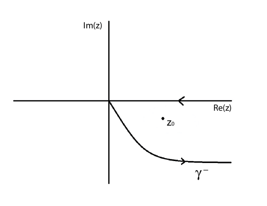
Figure 1: $\gamma^{-}$ is a curve in the lower half plane, starting at the origin, that together with the positive semi-axis of the real line encloses the pole $z_{0}$.

The meaning of the first spectral decomposition (10) is the following: let us assume that the functions $\varphi(\omega)=\langle\omega|\varphi\rangle$ and $\phi(\omega)=\langle\omega|\phi\rangle$ are analytically continuable to the upper and lower half of the complex plane, respectively. This, in particular, implies that $\varphi^{*}(\omega)=\langle\varphi|\omega\rangle$ admits analytic continuation to the lower half plane. The value of these functions at the point $z_{0}$ in the lower half plane is given by $\varphi^{*}(z_{0})=\langle\varphi|f^{D}\rangle$ and $\phi(z_{0})=\langle f^{G}|\phi\rangle$. The values of $\varphi^{*}(\omega)$ and $\phi(\omega)$ at the complex number $z$ with negative imaginary part are $\varphi^{*}(\omega)=\langle\varphi|z^{-}\rangle$ and $\phi(z)=\langle z^{+}|\phi\rangle$, respectively. Thus, what really has proper meaning is the value of $\langle\varphi|H|\phi\rangle$. Finally, $\gamma^{-}$ is a curve in the lower half plane, starting at the origin, that together with the positive semi-axis of the real line encloses the pole $z_{0}$ (see Fig. 1). Analogously, $\gamma^{+}$ is a curve in the upper half plane, starting at the origin, that together with the positive semi-axis of the real line encloses the pole $z^{*}_{0}$. The meaning of the second spectral decomposition in (10) is similar, but in the upper half plane.

A Friedrichs model with free Hamiltonian as in (6) and potential given by

$$V:=\sum_{k=1}^{N}\int_{0}^{\infty}f_{k}(\omega)\,[|\omega\rangle\langle k|+|k\rangle\langle\omega|]\,d\omega\,,$$ (11)

where the $f_{k}(\omega)$ are $N$ form factor functions (the total Hamiltonian is $H=H_{0}+\lambda V$), is expected to give $N$ resonance poles (although for a given value of $\lambda$, two of these poles may coincide at the same point, giving a double resonance pole). Thus, for a given value of $\lambda$, we have resonance poles at the points $z_{1},\dots,z_{N}$ and their complex conjugates, with respective decaying and growing Gamow vectors, $|f_{1}^{D}\rangle,\dots,|f_{N}^{D}\rangle$ and $|f_{1}^{G}\rangle,\dots,|f_{N}^{G}\rangle$. Then, the spectral decompositions (10) generalize to

$$H=\sum_{k=1}^{N}z_{k}\,|f_{k}^{D}\rangle\langle f_{k}^{G}|+\int_{\gamma^{-}}z\,|z^{-}\rangle\langle z^{+}|\,dz\,,\quad H=\sum_{k=1}^{N}z^{*}_{k}\,|f_{k}^{G}\rangle\langle f_{k}^{D}|+\int_{\gamma^{+}}z\,|z^{+}\rangle\langle z^{-}|\,dz\,.$$ (12)

The integral terms in (10) and (12) are responsible for the deviations of the exponential decay for very short (Zeno effect [3]) or very large values of time [4]. These effects are observable, although not easy to be observed [5, 6]. This means that, for the vast majority of experiments, they are not detected. Due to this reason, it makes sense to drop the integral term form (10) and (12), at least within a reasonable range of observations. Also, note that the spectral decompositions for $H$ either in (10) or in (12) are time reversal of each other, so that they are completely equivalent [34]. Therefore, one may take as an effective Hamiltonian, valid for the majority of observations, the following:

$$H=\sum_{k=1}^{N}z_{k}\,|f_{k}^{D}\rangle\langle f_{k}^{G}|\,.$$ (13)

As in the case $N=1$, we have that $H|f^{D}_{k}\rangle=z_{k}\,|f_{k}^{D}\rangle$, for $k=1,\dots,N$. Along (3), this suggests that

$$\langle f_{s}^{G}|f_{k}^{D}\rangle=\delta_{s,k}\,,\qquad s,k=1,\dots,N\,.$$ (14)

Analogously, $H|f^{G}_{k}\rangle=z^{*}_{k}\,|f_{k}^{G}\rangle$ for all $k$, so that if we take as effective Hamiltonian the second sum in (12), we have that $\langle f_{s}^{D}|f_{k}^{G}\rangle=\delta_{s,k}$, for all values of $s$ and $k$. Another property derived from this pseudometrics is that $\langle f_{k}^{D}|f_{s}^{D}\rangle=0=\langle f_{k}^{G}|f_{s}^{G}\rangle$.

Resonances may be considered as independent of each other, so that the Gamow vectors $|f_{1}^{D}\rangle,\dots,|f_{N}^{D}\rangle$ and $|f_{1}^{G}\rangle,\dots,|f_{N}^{G}\rangle$ may be assumed to be linearly independent. Then, we may assume that linear combinations of resonance states may belong either to the $N$ dimensional linear space, $\mathcal{H}_{N}^{D}$, spanned $|f_{1}^{D}\rangle,\dots,|f_{N}^{D}\rangle$ , or the space $\mathcal{H}_{N}^{G}$ spanned by $|f_{1}^{G}\rangle,\dots,|f_{N}^{G}\rangle$ or even to the $2N$ dimensional space, $\mathcal{H}_{2N}$, spanned by $|f_{1}^{D}\rangle,\dots,|f_{N}^{D}\rangle$ and $|f_{1}^{G}\rangle,\dots,|f_{N}^{G}\rangle$. Due to (14), the spaces $\mathcal{H}_{N}^{D}$ and $\mathcal{H}_{N}^{G}$ may be considered as duals of each other.

These ideas, along with (9), are the basis for the following comment. Assume that $|\psi\rangle$ and $|\varphi\rangle$ are arbitrary vectors in $\mathcal{\ H}_{N}^{D}$, so that

$$|\psi\rangle:=\sum_{k=1}^{N}a_{k}\,|f_{k}^{D}\rangle\,,\qquad|\varphi\rangle:=\sum_{k=1}^{N}b_{k}\,|f_{k}^{D}\rangle\,.$$ (15)

Let us evolve $|\varphi\rangle$ in time, with the evolution governed by the total Hamiltonian $H$. The value of this vector after a time $t$ has elapsed, is given by

$$|\varphi(t)\rangle=\sum_{k=1}^{N}b_{k}\,|f_{k}^{D}(t)\rangle\,,$$ (16)

where $|f_{k}^{D}(t)\rangle=e^{-itH}\,|f_{k}^{D}\rangle$ as in (9). Because of the duality between the spaces $\mathcal{H}_{N}^{D}$ and $\mathcal{H}_{N}^{G}$, the bra corresponding to the ket $|\psi\rangle$ is

$$\langle\psi|=\sum_{k=1}^{N}a^{*}_{k}\,\langle f_{k}^{G}|\,,$$ (17)

where the star denotes complex conjugation. The probability amplitude for the state $|\varphi(t)\rangle$ to be in the state $|\psi\rangle$ at time $t$ is given by

$$A(t)=\langle\psi|\varphi(t)\rangle=\sum_{k,s=1}^{N}a_{s}^{*}\,b_{k}\,\langle f_{s}^{G}|f_{k}^{D}(t)\rangle=\sum_{k,s=1}^{N}a_{s}^{*}\,b_{k}\,A_{s,k}(t)\,,$$ (18)

where,

$$A_{s,k}(t)=\langle f_{s}^{G}|e^{-itH}|f_{k}^{D}\rangle=e^{-iz_{k}t}\,\langle f_{s}^{G}|f_{k}^{D}\rangle=e^{-iz_{k}t}\delta_{s,k}=e^{-iE_{k}t}\,e^{-t\,\Gamma_{k}/2}\delta_{s,k}\,,$$ (19)

so that

$$A(t)=\sum_{k=1}^{N}a_{k}^{*}\,b_{k}\,e^{-iE_{k}t}\,e^{-t\,\Gamma_{k}/2}\,,$$ (20)

where $E_{k}$ and $-\Gamma_{k}/2$ are the real and imaginary parts of the resonance pole $z_{k}$, respectively.

Instead, we may have considered the vectors $|\psi\rangle$ and $|\varphi\rangle$ to be in the space $\mathcal{H}_{2N}$, and follow a similar reasoning. Formally, the results would have been different, since to (20), we had to add a similar term. If this were the case,

$$|\psi\rangle:=\sum_{k=1}^{N}a_{k}\,|f_{k}^{D}\rangle+\sum_{k=1}^{N}c_{k}\,|f^{G}_{k}\rangle\,,\qquad|\varphi\rangle:=\sum_{k=1}^{N}b_{k}\,|f_{k}^{D}\rangle+\sum_{k=1}^{N}d_{k}\,|f^{G}_{k}\rangle\,.$$ (21)

This construction, although useful for other purposes, may be incompatible with the formalism of Time Asymmetric Quantum Mechanics (TAQM) [29, 30, 31, 52], since in this formalism, time evolution for $|f_{k}^{D}\rangle$ is defined only for $t\geq 0$, while time evolution for $|f_{k}^{G}\rangle$ is only valid for $t\leq 0$. Nevertheless, a construction such that all growing and decaying Gamow vectors evolve rigorously for all values of time is possible [53], although this construction does not take into account the time asymmetry that is produced by decaying processes Thus, we consider the discussion on $\mathcal{H}_{N}^{D}$ as given above, as the most appropriate for our purposes.

2.2 Creation and annihilation operators

In this section we study the Friedrichs model in terms of the creation and annihilation operators. Its construction has been proposed, for instance, in [28]. The idea is the following: Let us assume that $a$ and $a^{\dagger}$ are the annihilation and creation of $|1\rangle$ in (3), respectively, and that $b_{\omega}$ and $b^{\dagger}_{\omega}$ play the same role in relation to $|\omega\rangle$. Then, the Friedrichs free Hamiltonian $H_{0}$ written in terms of these operators is a contribution of two terms $H_{0}=H_{A}+H_{R}$, where [28],

$$H_{A}:=\omega_{0}\,a^{\dagger}\,a\,,\qquad H_{R}:=\int_{0}^{\infty}d\omega\,\omega\,b_{\omega}^{\dagger}\,b_{\omega}\,,$$ (22)

and the interaction is now written as

$$H_{I}=\lambda\int_{0}^{\infty}d\omega\,f(\omega)(a^{\dagger}\,b_{\omega}+a\,b^{\dagger}_{\omega})\,,$$ (23)

where $\lambda$ is the coupling constant and $f(\omega)$ the form factor. Again, the total Hamiltonian is $H=H_{0}+H_{I}=H_{A}+H_{R}+H_{I}$. The function

$$\eta(z):=\omega_{0}-z-\int_{0}^{\infty}d\omega\;\frac{\lambda^{2}\,f^{2}(\omega)}{\omega-z}\,,$$ (24)

is analytic with a branch cut on the positive semi-axis $[0,\infty)$. We denote its limits on this semi-axis from above to below and from below to above as $\eta^{+}(\omega):=\eta(\omega+i0)$ and $\eta^{-}(\omega):=\eta(\omega-i0)$, respectively. Then, a “diagonalization” of the total Hamiltonian $H$ is given by [28]

$$H=z_{0}\,(A^{\dagger})_{\mathrm{in}}\,A_{\mathrm{out}}+\int_{0}^{\infty}d\omega\,\omega\;\frac{\eta^{+}(\omega)}{\eta^{-}(\omega)}\;(\tilde{B}^{\dagger}_{\omega})_{\mathrm{in}}\,(\tilde{B}_{\omega})_{\mathrm{out}}\,.$$ (25)

Here, $(A^{\dagger})_{\mathrm{in}}$ and $A_{\mathrm{out}}$ are the creation and annihilation of the Gamow state from a vacuum $|0\rangle$, so that

$$|f^{D}\rangle=(A^{\dagger})_{\mathrm{in}}\,|0\rangle\,,\quad|0\rangle=A_{\mathrm{out}}|f^{D}\rangle\,,\quad A_{\mathrm{out}}|0\rangle=0\,,\quad[A_{\mathrm{out}},A^{\dagger}_{\mathrm{in}}]=1\,,$$ (26)

while $(\tilde{B}^{\dagger}_{\omega})_{\mathrm{in}}$ and $(\tilde{B}_{\omega})_{\mathrm{out}}$ are creation and annihilation operators of states in the continuum, which were defined in [28]. The latter do not have here any interest for us, as we are solely interested in the resonance behavior. The subscripts “in” and “out” come from scattering theory and do not play any role in our discussion here, so that we will omit them. Thus, the effective Hamiltonian, which concerns only to the presence of resonances is given by $H=z_{0}\,A^{\dagger}\,A$ in our notation.

Now, rename $|f_{1}^{D}\rangle:=|f^{D}\rangle$ and define $|f_{n}^{D}\rangle:=(A^{\dagger})^{n}\,|f_{1}^{D}\rangle$. If we denote by $N:=A^{\dagger}\,A$, it readily comes that

$$N|f_{n}^{D}\rangle=n\,|f_{n}^{D}\rangle\,,\qquad H|f_{n}^{D}\rangle=nz_{0}\,|f_{n}^{D}\rangle\,,$$ (27)

which formally yields

$$e^{-itH}\,|f_{n}^{D}\rangle=e^{-itnz_{0}}\,|f_{n}^{D}\rangle\,.$$ (28)

In the next section, we are going to apply the formalism of Gamow vectors to the Loschmidt echo.

3 Loschmidt echo and Gamow vectors

We consider a quantum system in an initial state $|\alpha(0)\rangle$. Let us suppose that this initial state is evolved during a time interval $\tau$, and then it is evolved backwards during the same interval $\tau$. We denote the final state as $|\alpha(2\tau)\rangle$. At this point, we can compare the initial state $|\alpha(0)\rangle$ with the final state $|\alpha(2\tau)\rangle$. When the time-reversal procedure is perfectly implemented and the time-evolution is unitary, both states are exactly the same. However, when the time-reversal implementation is imperfect, there exist some degree of discrepancy between the states. One way to quantify this discrepancy is using the Loschmidt echo. If the time-evolution of the quantum system is given by the operator $U_{1}(\tau)=e^{-\frac{i}{\hbar}H_{1}\tau}$, we define the decay rate by

$$M(\tau):=|\langle\alpha(0)|U_{2}(\tau)\,U_{1}(\tau)|\alpha(0)\rangle|^{2}\,.$$ (29)

where $U_{2}(\tau)=e^{\frac{i}{\hbar}H_{2}\tau}$, and $H_{2}$ is a perturbation of $H_{1}$.

It is easy to see that $M(\tau)=1$, when there is no discrepancy, and $M(\tau)=0$, when the discrepancy is maximal. In particular, $M(\tau)$ is maximal when the time evolution is unitary and the time reversal is perfect. In the usual approach, it is assumed that the time evolution is unitary, but the time reversal is imperfect, i.e., the backward Hamiltonian is not exactly opposite to the forward Hamiltonian. In this work, we adopt an alternative approach. We consider a perfectly implemented time reversal, but a non-unitary time evolution.

In order to illustrate our approach, let us discuss how the time reversal is implemented in laboratory realizations. Consider the case of a crystal under the action of an external magnetic field oriented in the $\hat{z}$ direction (as discussed in [54]). After applying $U_{1}$ during a time interval $\tau$, the orientation of the external magnetic field is rotated and a new Hamiltonian $H_{2}$ is obtained. The action of $H_{2}$ during a time interval $\tau$ is formally equivalent to the time reversion.

In the standard approach, the new Hamiltonian $H_{2}$ is represented as a perturbation of the opposite initial Hamiltonian $H_{1}$. In our alternative description, we assume that evolutions are non-unitary. This is the mathematical expression of the assumption that the system has an intrinsic irreversibility which is not caused by the environment. The irreversibility is formally represented by the decaying exponential factor related to the time evolution of a Gamow vector.

Let us describe how the second Hamiltonian $H_{2}$ is modeled under these assumptions. In the crystal example, the magnetic field is changed from $\hat{z}$ to $-\hat{z}$. After this transformation, the signs of the real parts of the eigenvalues change, but the resonances remain the same, because they are related to internal degrees of freedom, and have nothing to do with the orientation of the system respect to the laboratory. Thus, the Hamiltonian $H_{2}$ changes its complex eingenvalues as follows: $z=\omega-\frac{i}{2}\Gamma\longrightarrow-z^{*}=-\omega-\frac{i}{2}\Gamma$. Physically, this means that reversing the physical process do not change the decay factor of the dynamical law. Our description of what happens in the laboratory allows to explain why the initial state is not recovered. The decaying behavior of the Gamow vectors explains the Lodschmit echo. Therefore, the forward and backward evolution operators, $U_{1}(\tau)$ and $U_{2}(\tau)$ respectively, have the following form:

$$U_{1}(\tau) =\sum_{n=0}^{N}e^{-\frac{i\tau}{\hbar}z_{n}}\,|f_{n}^{D}\rangle\langle f_{n}^{G}|\,.$$ (30)

$$U_{2}(\tau) =\sum_{n=0}^{N}e^{\frac{i\tau}{\hbar}z^{*}_{n}}\,|f_{n}^{D}\rangle\langle f_{n}^{G}|\,.$$ (31)

Notice that, for all Gamow states $\{|f_{n}^{D}\rangle\}$, we have

$$U_{1}(\tau)|f_{n}^{D}\rangle=e^{-\frac{i\tau}{\hbar}z_{n}}\,|f_{n}^{D}\rangle\qquad\mathrm{\ and}\qquad U_{2}(\tau)|f_{n}^{D}\rangle=e^{\frac{i\tau}{\hbar}z^{*}_{n}}\,|f_{n}^{D}\rangle\,,$$ (32)

$U_{2}(\tau)U_{1}(\tau)$ is well defined, and it is different from the identity. Applying this time evolution in equation (29), we obtain

$$\langle\alpha(0)|U_{2}(\tau)U_{1}(\tau)|\alpha(0)\rangle = \langle\alpha(0)|\sum_{n=0}^{N}e^{\frac{i\tau}{\hbar}z_{n}^{\ast}}\,|f_{n}^{D}\rangle\langle f_{n}^{G}|\sum_{m=0}^{N}e^{-\frac{i\tau}{\hbar}z_{m}}\,|f_{m}^{D}\rangle\langle f_{m}^{G}|\alpha(0)\rangle=$$ (33)

$$= \sum_{n=0}^{N}e^{\frac{i\tau}{\hbar}(z_{n}^{\ast}-z_{n})}\langle\alpha(0)|f_{n}^{D}\rangle\langle f_{n}^{G}|\alpha(0)\rangle=$$

$$= \sum_{n=0}^{N}e^{-\tau\gamma_{n}/\hbar}\langle\alpha(0)|f_{n}^{D}\rangle\langle f_{n}^{G}|\alpha(0)\rangle\,.$$

Let us suppose that the initial state is a superposition of the Gamow vectors $|f_{n}^{D}\rangle$

$$|\alpha(0)\rangle=\sum_{n=0}^{N}a_{n}\;|f_{n}^{D}\rangle,$$ (34)

then

$$\langle\alpha(0)|=\sum_{n=0}^{N}a^{*}_{n}\;\langle f_{n}^{G}|.$$ (35)

Now, using the relations (14), we obtain

$$\langle\alpha(0)|U_{2}(\tau)U_{1}(\tau)|\alpha(0)\rangle=\sum_{n=0}^{N}e^{-\tau\gamma_{n}/\hbar}|a_{n}|^{2}.$$ (36)

This result shows that the Loschmidt echo decays with time, and its decay depends on the initial conditions $a_{n}$ and the characteristic times $\gamma_{n}^{-1}$.

The decay of the Loschmidt echo has different regimes, such as parabolic, exponential, gaussian among others [55, 56, 57, 58, 59, 60, 61]. The most simple case of equation (36) is when there is only one characteristic time, or when the initial conditions are such that only one mode is activated. In these cases, it is obtained a pure exponential decay. In this way, Gamow vectors can be used to model experimental situations. In the general case, the combination of exponential functions with different characteristic times leads to more diverse time evolutions.

4 Decoherence and Loschmidt echo

So far we have seen how the Gamow vectors can be used to describe the Loschmidt echo. We saw that the type of decay of the quantity $M(\tau)$ is determined by the complex part of the Hamiltonian eigenstates and the initial conditions. In what follows we will show that there is a close relationship between the Loschmidt echo and the quantum decoherence phenomenon. This connection is because the decoherence time is also related with the imaginary part of the Hamiltonian eigenstates and the initial conditions.

To study the decoherence process in the Friedrich model, it is necessary to introduce the quasi coherent states, since they form the so-called privileged basis. Quasi-coherent states have been discussed in [62, 63, 64].

4.1 Initial conditions

For systems having an infinite number of resonances, it is possible in principle to define coherent resonance states. This states should have the following form for each complex number $z\in\mathbb{C}$:

$$|z^{D}\rangle=e^{-|z|^{2}/2}\sum_{k=0}^{\infty}\frac{z^{n}}{\sqrt{n!}}\,|f_{k}^{D}\rangle\,.$$ (37)

These coherent states should be eigenvectors with eigenvalue $z$ of a annihilation operator $B^{-}$, satisfying $B^{-}|f_{k}^{D}\rangle=k|f_{k-1}^{D}\rangle$, for all $k\in\mathbb{N}$, where $|f_{0}^{D}\rangle=0$, so that $B^{-}|z^{D}\rangle=z\,|z^{D}\rangle$. This can be implemented for some exactly solvable models for resonances, like the high barrier Pöschl-Teller one dimensional model [65, 66].

Unfortunately, up to our knowledge, nobody has constructed a solvable Friedrichs model with an infinite number of resonance poles. Let us assume that we have $N+1$ resonances with decaying Gamow vectors $|f_{0}^{D}\rangle,\dots,|f_{N}^{D}\rangle$. By definition, a quasi coherent state at time $t=0$ is a vector of the form:

$$|\alpha_{1}(0)\rangle:=\left(\sum_{k=0}^{N}\frac{|\alpha_{1}(0)|^{2k}}{k!}\right)^{-1/2}\sum_{n=0}^{N}\frac{(\alpha_{1}(0))^{n}}{\sqrt{n!}}\;|f_{n}^{D}\rangle\,,$$ (38)

where $\alpha_{1}(0)$ is a given complex number. Note that for $N$ going to infinity (38) acquires the form (37), hence the name of quasi-coherent state. Analogously, for any other complex number $\alpha_{2}(0)$, we have

$$|\alpha_{2}(0)\rangle:=\left(\sum_{k=0}^{N}\frac{|\alpha_{2}(0)|^{2k}}{k!}\right)^{-1/2}\sum_{n=0}^{N}\frac{(\alpha_{2}(0))^{n}}{\sqrt{n!}}\;|f_{n}^{D}\rangle\,.$$ (39)

Notice that, in a rough approximation, we may consider the pair of vectors $\{|\alpha_{1}(0)\rangle,|\alpha_{2}(0)\rangle\}$ as the Moving Preferred Basis in the sense of [67]. The approximation is rough because we have taken $t=0$, therefore it is not properly a moving basis. It is certainly efficient in the range of extremely short decoherence times $t_{D}$ compared to relaxation time $t_{R}$, i.e., $t_{D}<<t_{R}$. In this sense, the choice $t_{D}=0$ is a workable approximation. Let us consider an arbitrary normalized linear combination of these two vectors; $|\Phi(0)\rangle:=a|\alpha_{1}(0)\rangle+b|\alpha_{2}(0)\rangle$. Its corresponding density matrix is given by

$$\rho_{0}= |\Phi(0)\rangle\langle\Phi(0)|=$$

$$= |a|^{2}\,|\alpha_{1}(0)\rangle\langle\alpha_{1}(0)|+ab^{*}\,|\alpha_{1}(0)\rangle\langle\alpha_{2}(0)|+a^{*}b\,|\alpha_{2}(0)\rangle\langle\alpha_{1}(0)|+|b|^{2}\,|\alpha_{2}(0)\rangle\langle\alpha_{2}(0)|\,.$$ (40)

Note that, if $i=1,2$,

$$\langle\alpha_{i}(0)|=\left(\sum_{k=0}^{N}\frac{|\alpha_{i}(0)|^{2k}}{k!}\right)^{-1/2}\sum_{n=0}^{N}\frac{(\alpha^{*}_{i}(0))^{n}}{\sqrt{n!}}\;\langle f_{n}^{G}|\,.$$ (41)

After a time $t>0$, the state becomes

$$\rho(t)= |\Phi(t)\rangle\langle\Phi(t)|=$$

$$= |a|^{2}\,|\alpha_{1}(t)\rangle\langle\alpha_{1}(t)|+ab^{*}\,|\alpha_{1}(t)\rangle\langle\alpha_{2}(t)|+a^{*}b\,|\alpha_{2}(t)\rangle\langle\alpha_{1}(t)|+|b|^{2}\,|\alpha_{2}(t)\rangle\langle\alpha_{2}(t)|\,.$$ (42)

The expression in the second row in (4.1) contains four terms. The sum of the second and third terms is called the non-diagonal part that we intend to analyze next.

4.2 Decoherence

Let us denote the sum of the second and third term in (4.1) as $\rho^{\mathrm{ND}}(t)$. Under the condition of macroscopicity, which is introduced below, the non-diagonal terms in (4.1) approximately satisfy the following relation:

$$\rho^{\mathrm{ND}}(t)=\rho^{\mathrm{ND}}_{12}(t)\,|\alpha_{1}(0)\rangle\langle\alpha_{2}(0)|+\rho^{\mathrm{ND}}_{21}(t)\,|\alpha_{2}(0)\rangle\langle\alpha_{1}(0)|\,.$$ (43)

This is not true in the general case as one may check by a direct calculation on $|\alpha_{1}(t)\rangle\langle\alpha_{2}(t)|=e^{-itH}\,|\alpha_{1}(0)\rangle\langle\alpha_{2}(0)|\,e^{itH}$.

In order to show (43), we should make the hypothesis of the macroscopicity condition, which means that the peaks of both approximate Gaussians are far from each other. This means that $|\alpha_{1}^{*}(0)-\alpha_{2}(0)|$ is very large (we will consider $\alpha_{1}(0)$ as a real value). Notice that, under this hypothesis, the states of the preferred basis $\{|\alpha_{1}(0)\rangle,|\alpha_{2}(0)\rangle\}$ are approximately orthogonal or quasi-orthogonal, which means that

$$\langle\alpha_{1}(0)|\alpha_{2}(0)\rangle=\langle\alpha_{2}(0)|\alpha_{1}(0)\rangle^{*}\approx 0\,.$$ (44)

To show (44), we first note that after (39) and (41) we have that

$$\langle\alpha_{1}(0)|\alpha_{2}(0)\rangle=\left(\sum_{k=0}^{N}\frac{|\alpha_{1}(0)|^{2k}}{k!}\right)^{-1/2}\left(\sum_{k=0}^{N}\frac{|\alpha_{2}(0)|^{2k}}{k!}\right)^{-1/2}\sum_{n=0}^{N}\frac{(\alpha_{1}^{*}(0)\,\alpha_{2}(0))^{n}}{n!}\,.$$ (45)

Then, let us use the Cauchy product and the binomial formula on the two first factors on the right hand side of (45), so as to obtain:

$$\langle\alpha_{1}(0)|\alpha_{2}(0)\rangle=\left(\sum_{k=0}^{N}\frac{(|\alpha_{1}(0)|^{2}+|\alpha_{2}(0)|^{2})^{k}}{k!}\right)^{-1/2}\sum_{n=0}^{N}\frac{(\alpha_{1}^{*}(0)\,\alpha_{2}(0))^{n}}{n!}\,.$$ (46)

Repeating the procedure, we obtain

$$\langle\alpha_{1}(0)|\alpha_{2}(0)\rangle=\sum_{n=0}^{N}\frac{1}{n!}\left(-\frac{1}{2}(|\alpha_{1}(0)|^{2}+|\alpha_{2}(0)|^{2}-2\alpha_{1}^{*}(0)\alpha_{2}(0))\right)^{n}$$

$$=\sum_{n=0}^{N}\frac{1}{n!}\left(-\frac{(\alpha_{1}^{*}(0)-\alpha_{2}(0))^{2}}{2}\right)^{n}\,.$$ (47)

Clearly after (4.2), for $|\alpha_{1}^{*}(0)-\alpha_{2}(0)|$ very large, we obtain (44). For this case, let us define

$$\rho_{12}^{\mathrm{ND}}(t):=\langle\alpha_{1}(0)|\rho(t)|\alpha_{2}(0)\rangle\,,\quad\rho_{21}^{\mathrm{ND}}(t):=\langle\alpha_{2}(0)|\rho(t)|\alpha_{1}(0)\rangle\,,$$ (48)

where $\rho(t)$ has been introduced in (4.1), from which we have that

$$\rho_{12}^{\mathrm{ND}}(t)=ab^{*}\,\langle\alpha_{1}(0)|\alpha_{1}(t)\rangle\langle\alpha_{2}(t)|\alpha_{2}(0)\rangle+a^{*}b\,\langle\alpha_{1}(0)|\alpha_{2}(t)\rangle\langle\alpha_{1}(t)|\alpha_{2}(0)\rangle\,,$$

$$\rho_{21}^{\mathrm{ND}}(t)=ab^{*}\,\langle\alpha_{2}(0)|\alpha_{1}(t)\rangle\langle\alpha_{2}(t)|\alpha_{1}(0)\rangle+a^{*}b\,\langle\alpha_{2}(0)|\alpha_{2}(t)\rangle\langle\alpha_{1}(t)|\alpha_{1}(0)\rangle\,.$$ (49)

In order to compute (4.2), let us follow the notation used in (15), (16) and (17). In what follows, we will assume that the numbers $\alpha_{1}(0)$ and $\alpha_{2}(0)$ are real. If we choose $|\psi\rangle:=|\alpha_{1}(0)\rangle$ and $|\varphi(t)\rangle:=|\alpha_{1}(t)\rangle$, and take into account (38) and (41), we have that the coefficients $a_{k}$ and $b_{k}$ in (15) and (16) have the following form:

$$a_{k}=\frac{\left(\alpha_{1}(0)\right)^{k}}{\sqrt{k!}}\,e^{-\frac{1}{2}\,|\alpha_{1}(0)|^{2}}\,,\qquad b_{k}=\frac{\left(\alpha_{1}(0)\right)^{k}}{\sqrt{k!}}\,e^{-\frac{1}{2}\,|\alpha_{1}(0)|^{2}}\,,$$ (50)

so that,

$$\left\langle\alpha_{1}(0)|\alpha_{1}(t)\right\rangle=e^{-\left|\alpha_{1}(0)\right|^{2}}\sum_{n=0}^{N}\frac{\left(\left|\alpha_{1}(0)\right|^{2}\right)^{n}}{n!}e^{-iz_{n}t}\,.$$ (51)

Then, we take $|\psi\rangle:=|\alpha_{1}(0)\rangle$ and $|\varphi(t)\rangle:=|\alpha_{2}(t)\rangle$, which gives after (39) and (41) that

$$a_{n}=\frac{\left|\alpha_{1}(0)\right|^{n}}{\sqrt{n!}}\,e^{-\frac{1}{2}\,|\alpha_{1}(0)|^{2}}\,,\qquad b_{n}=\frac{\left|\alpha_{2}(0)\right|^{n}}{\sqrt{n!}}\,e^{-\frac{1}{2}\,|\alpha_{2}(0)|^{2}}\,,$$ (52)

so that

$$\left\langle\alpha_{1}(0)|\alpha_{2}(t)\right\rangle=e^{-\frac{1}{2}\,\{|\alpha_{1}(0)|^{2}+\left|\alpha_{2}(0)\right|^{2}\}}\sum_{n=0}^{N}\frac{\left(\left|\alpha_{1}(0)\right|\left|\alpha_{2}(0)\right|\right)^{n}}{n!}e^{-iz_{n}t}\,.$$ (53)

In the third place, we choose $|\psi\rangle=|\alpha_{2}(0)\rangle$ and $|\varphi(t)\rangle=|\alpha_{1}(t)\rangle$, which give

$$a_{n}=\frac{\left(\alpha_{2}(0)\right)^{n}}{\sqrt{n!}}\,e^{-\frac{1}{2}\,|\alpha_{2}(0)|^{2}}\,,\qquad b_{n}=\frac{\left(\alpha_{1}(0)\right)^{n}}{\sqrt{n!}}\,e^{-\frac{1}{2}\,|\alpha_{1}(0)|^{2}}\,,$$ (54)

so that

$$\left\langle\alpha_{2}(0)|\alpha_{1}(t)\right\rangle=e^{-\frac{1}{2}\,\{|\alpha_{1}(0)|^{2}+\left|\alpha_{2}(0)\right|^{2}\}}\sum_{n=0}^{N}\frac{\left(\left|\alpha_{1}(0)\right|\left|\alpha_{2}(0)\right|\right)^{n}}{n!}e^{-iz_{n}t}$$ (55)

Finally, the choice $|\psi\rangle:=|\alpha_{2}(0)\rangle$ and $|\varphi(t)\rangle:=|\alpha_{2}(t)\rangle$ gives

$$a_{n}=\frac{\left(\alpha_{2}(0)\right)^{n}}{\sqrt{n!}}\,e^{-\frac{1}{2}\,|\alpha_{2}(0)|^{2}}\,,\qquad b_{n}=\frac{\left(\alpha_{2}(0)\right)^{n}}{\sqrt{n!}}\,e^{-\frac{1}{2}\,|\alpha_{2}(0)|^{2}}\,,$$ (56)

so that,

$$\left\langle\alpha_{2}(0)|\alpha_{2}(t)\right\rangle=e^{-\left|\alpha_{2}(0)\right|^{2}}\sum_{n=0}^{N}\frac{\left(\left|\alpha_{2}(0)\right|^{2}\right)^{n}}{n!}\,e^{-iz_{n}t}\,.$$ (57)

So far, we have presented our discussion on the quasi-coherent states based in the properties of the Friedrichs model. In the next sections, we will present another approach, in such a way that the above discussion can be applied to decoherence and the Loschmidt echo.

In this case, we may redefine (38) and (39), and then

$$|\alpha_{i}(0)\rangle=e^{-\frac{1}{2}\,|\alpha_{i}(0)|^{2}}\sum_{n=0}^{\infty}\frac{(\alpha_{i}(0))^{n}}{\sqrt{n!}}\,|f_{n}^{D}\rangle\,,\qquad i=1,2\,.$$ (58)

Following the discussion in [67], we repeat the procedure outlined in Section 3.1 to the present situation. Now, $z_{n}=nz_{0}$ and the sum over $n$ goes to infinite. As initial values, we choose

$$\alpha_{1}(0)=0\,,\qquad\alpha_{2}(0)\neq 0.$$ (59)

The macroscopicity condition now means that $\alpha_{2}(0)>>1$. Then, equations (51), (53), (55) and (57) now give, respectively,

$$\langle\alpha_{1}(0)|\alpha_{1}(t)\rangle=1\,,\quad\langle\alpha_{1}(0)|\alpha_{1}(t)\rangle=e^{-\frac{1}{2}\,|\alpha_{2}(0)|^{2}}\approx 0\,,\quad\langle\alpha_{2}(0)|\alpha_{1}(t)\rangle=e^{-\frac{1}{2}\,|\alpha_{2}(0)|^{2}}\approx 0\,,$$ (60)

$$\langle\alpha_{2}(0)|\alpha_{2}(t)\rangle=\exp\left\{-|\alpha_{2}(0)|^{2}\right\}\,e^{-iz_{0}t}\,.$$ (61)

Consequently, the non-diagonal coefficients defined in (43), and explicitly given in its general form in (4.2), take in this case the approximate following values:

$$\rho_{12}^{\mathrm{ND}}(t)\approx ab^{*}\,\exp\left\{-|\alpha_{2}(0)|^{2}\right\}\,e^{-iz_{0}t}\,,$$ (62)

and

$$\rho_{21}^{\mathrm{ND}}\approx a^{*}b\,\exp\left\{-|\alpha_{2}(0)|^{2}\right\}\,e^{-iz_{0}t}\,.$$ (63)

We see that as $t\longmapsto\infty$, the non-diagonal terms are of the order of $\exp\{-|\alpha_{2}(0)|^{2}\}\approx 0$, which shows decoherence in the preferred basis.

This formalism may be extended to a Friedrichs model with $N+1$ bound states for $H_{0}$ and, hence, with $N+1$ resonance poles, $z_{0},\dots,z_{N}$. In this case, equations (62) and (63) take the following forms, respectively,

$$\rho_{12}^{\mathrm{ND}}(t)\approx ab^{*}\,\exp\left\{-|\alpha_{2}(0)|^{2}\right\}\sum_{n=0}^{N}\frac{(|\alpha_{2}(0)|^{2})^{n}}{n!}\,e^{-\frac{i}{\hbar}z_{n}t}$$ (64)

and

$$\rho_{12}^{\mathrm{ND}}(t)\approx a^{*}b\,\exp\left\{-|\alpha_{2}(0)|^{2}\right\}\sum_{n=0}^{N}\frac{(|\alpha_{2}(0)|^{2})^{n}}{n!}\,e^{-\frac{i}{\hbar}z_{n}t}\,.$$ (65)

These results show that the non-diagonal elements of the density matrix go to cero when time goes to infinite. This process is called decoherence. In previous works [68, 69, 70], more examples of this phenomenon have been studied using non-hermitian Hamiltonians.

As is known, the decoherence is an irreversible process [71], therefore there is some kind of irreversibility in this model. This motivates us to study more aspects of the irreversibility of this model. In particular, in this work we are interested in the Loschmidt echo phenomenon.

4.3 Loschmidt echo

As we have seen in equation (33), $M(\tau)$ can be expressed as

$$M(\tau)=\sum_{n=0}^{N}e^{-\tau\gamma_{n}/\hbar}\langle\alpha_{2}(0)|f_{n}^{D}\rangle\langle f_{n}^{G}|\alpha_{2}(0)\rangle\,.$$ (66)

Now, using the identity (39) and relations (14), we have that

$$\langle f_{n}^{G}|\alpha_{2}(0)\rangle=\left(\sum_{k=0}^{N}\frac{|\alpha_{2}(0)|^{2k}}{k!}\right)^{-1/2}\frac{(\alpha_{2}(0))^{n}}{\sqrt{n!}}\,.$$ (67)

Analogously, using (41), one has that

$$\langle\alpha_{2}(0)|f_{n}^{D}\rangle=\left(\sum_{k=0}^{N}\frac{|\alpha_{2}(0)|^{2k}}{k!}\right)^{-1/2}\frac{(\alpha_{2}^{*}(0))^{n}}{\sqrt{n!}}\,,$$ (68)

so that

$$\langle\alpha_{2}(0)|M(\tau)|\alpha_{2}(0)\rangle=A\sum_{n=0}^{N}\frac{|\alpha_{2}(0)|^{2n}}{n!}e^{-\tau\gamma_{n}/\hbar}$$

with

$$A=\left(\sum_{k=0}^{N}\frac{|\alpha_{2}(0)|^{2k}}{k!}\right)^{-1}\approx\left(\sum_{k=0}^{\infty}\frac{|\alpha_{2}(0)|^{2k}}{k!}\right)^{-1}=\exp\{-|\alpha_{2}(0)|^{2}\}\,$$ (69)

and the latter approximation makes sense for $N$ large, so that

$$\langle\alpha_{2}(0)|M(\tau)|\alpha_{2}(0)\rangle\approx e^{-|\alpha_{2}(0)|^{2}}\sum_{n=0}^{N}\frac{|\alpha_{2}(0)|^{2n}}{n!}e^{-\tau\gamma_{n}/\hbar}$$ (70)

Comparing equation (70) with equations (64) and (65), it is observed that, in both cases, the decay rate is related to the imaginary part of the Hamiltonian eigenvalues. In the first case, the decay is accompanied by an oscillation, while in the second case it is not. In both cases the characteristic times of the exponential decays are the same.

The result shows that there is an intimate relationship between both phenomena. This connection is not surprising since the Loschmidt echo and quantum decoherence can be considered as two expressions of the irreversibility of quantum systems. However, it is of significant importance since it links two phenomena that have been studied separately.

5 Conclusions

The Gamow vectors formalism has been developed in order to give a mathematical description of quantum decay phenomena, such as radioactive phenomena, scattering or decoherence. In this paper we extend the scope of this formalism. We use the Gamow vectors to describe the Loschmidt echo.

The irreversible character of the Loschmidt echo can be studied in two manners. One approach considers that the time evolution is perfectly unitary, but there are imperfections in the implementation of the time reversal operation. The backward and forward evolution process are governed by two slightly different Hamiltonians. This can be attributed to the noise introduced by the environment. The other approach is to assume that the time evolution operator is not unitary, which introduces an intrinsic irreversibility of the time evolution. This kind of evolutions are well represented by the Gamow vector formalism.

In this paper, we adopted the second approach: we used Gamow vectors to describe the Loschmidt echo phenomenon. We showed that the characteristic time of this process is directly associated with the resonances of the analytical continuation of the Hamiltonian. Moreover, we proved that the type of decay obtained is related to the number of resonances of the system and their relative weight in the initial state.

Additionally, we compared this phenomenon with another well known one: the decoherence process. In this case, the resonances are related to the decoherence and relaxation times. We considered a toy model based on the Friedrichs model. We showed that choosing as the initial state a superposition of two quasi-coherent states, and taking into account the macroscopicity condition, decoherence and Loschmidt echo can be described simultaneously. Moreover, the characteristic time of the Loschmidt echo is related with the decoherence time, since both times are determined by the same resonances. Therefore, we have concluded that, under our hypothesis, the Loschmidt echo and decoherence, can be considered as two aspects of the same phenomenon, and that there is a mathematical relation between their corresponding characteristic times.

References

- [1] G. Gamow, Zur Quantentheorie des Atomkernes, Z. Phys, 51, 204-212 (1928).
- [2] L. Fonda, G.C. Ghirardi, A. Rimini, Decay theory of unstable quantum systems, Rep. Progr. Phys., 41, 587-631 (1978).
- [3] B. Misra, E.C.G. Sudarshan, Zeno’s paradox in quantum theory, J. Math. Phys., 18 (4), 756-763 (1977).
- [4] L. Khalfin, Contribution to the decay theory of a quasi-stationary state, SOVIET PHYSICS JETP-USSR, 6 (6), 1053-1063 (1958).
- [5] M.C. Fischer, B. Gutiérrez-Medina, M.G. Raizen, Observation of the quantum Zeno and anti-Zeno effects in an unstable system, Phys. Rev. Lett., 87, 40402 (2001).
- [6] C. Rothe, S.L. Hintschich, A.P. Monkman, Violation of the exponential decay law at long times, Phys. Rev. Lett., 96, 163601 (2006).
- [7] N. Nakanishi, A theory of clothed unstable particles, Rep. Progr. Phys., 19 (6), 607-621 (1958).
- [8] A. Bohm, Quantum Mechanics: Foundations and Applications, Springer Verlag, Berlin, New York, 1993.
- [9] A. Bohm, Decaying states in the rigged Hilbert space formulation of Quantum Mechanics, J. Math. Phys., 21 (5), 1040-1043 (1980).
- [10] A. Bohm, Resonance poles and Gamow vectors in the rigged Hilbert space formulation of Quantum Mechanics, 22 (12), 2813-2823 (1981).
- [11] I. M. Gelfand and N.Ya.Vilenkin, Generalized Functions: Applications to Harmonic Analysis (Academic, NewYork, 1964).
- [12] R. Ramírez, M Reboiro, Dynamics of finite dimensional non-hermitian systems with indefinite metric, J. Math. Phys., 60, 012106 (2019).
- [13] A. Bohm, The Rigged Hilbert Space and Quantum Mechanics, Springer Lecture Notes in Physics (Springer, Berlin, 1978), Vol. 78.
- [14] J. E. Roberts, Rigged Hilbert spaces in quantum mechanics, Commun. Math. Phys. 3, 98-119 (1966).
- [15] J. P. Antoine, Dirac formalism and symmetry problems in quantum mechanics, J. Math. Phys. 10, 53-69 (1969).
- [16] O. Melsheimer, Rigged Hilbert space formalism as an extended mathematical formalism for quantum systems. I General Theory. J. Math. Phys. 15, 902-916 (1974).
- [17] M. Gadella, F. Gómez, A unified mathematical formalism for the Dirac formulation of quantum mechanics, Foundations of Physics, 32, 815-869 (2002).
- [18] M. Gadella, F. Gómez, On the mathematical basis of the Dirac formulation of Quantum Mechanics, Int. J. Theor. Phys., 42, 2225-2254 (2003).
- [19] G. Bellomonte, S. di Bella, C. Trapani, Operators in rigged Hilbert spaces: some spectral properties, J. Math. Anal. Appl., 411, 931-946 (2014).
- [20] A. Bohm, M. Gadella, Dirac kets, Gamow vectors and Gelfand triplets, Springer Lecture Notes in Physics 348, Springer, New York 1989.
- [21] O. Civitarese, M. Gadella, Physical and mathematical aspects of Gamow states, Phys. Rep., 396, 41-113 (2004).
- [22] I.E. Antoniou, I. Prigogine, Intrinsic irreversibility and integrability of dynamics, Phys. A, 192 (3), 443-464 (1994).
- [23] Z. Suchanecki, I. Antoniou, S. Tasaki, O.F. Bandtlow, Rigged Hilbert spaces for chaotic dynamical systems, J. Math. Phys., 37 (11), 5837-5847 (1996).
- [24] I. Antoniou, Z. Suchanecki, R. Laura, S. Tasaki, Intrinsic irreversibility of quantum systems with diagonal singularity, Phys. A: Stat. Mech. Appl., 241, (3-4), 737-772 (1997).
- [25] I. Antoniou, L. Dmitrieva, Y. Kuperin, Y. Melnikov, Resonances and the extension of dynamics to rigged Hilbert space, Comp. Math. Appl., 34 (5-6), 399-425 (1997).
- [26] I. Antoniou, M. Gadella, I. Prigogine, G.P. Pronko, Relativistic Gamow vectors, J. Math. Phys., 39 (6), 2995-3018 (1998).
- [27] T. Petrosky, I. Prigogine, Thermodynamic limit, Hilbert space and breaking of time symmetry, Chaos, Solitons and Fractals, 11 (1-3), 373-382 (1997).
- [28] I.E. Antoniou, M. Gadella, E. Karpov, I. Prigogine, G. Pronko, Gamow algebras, Chaos, Solitons and Fractals, 12, 2757-2775 (2001).
- [29] A. Bohm, Time-asymmetric quantum physics, Phys. Rev. A, 60 (2), 861-876, 1999.
- [30] A. Bohm, F. Erman, H. Uncu, Resonance Phenomena and time asymmetric quantum mechanics, Turkish Journal of Physics, 35 (3), 209-240 (2011).
- [31] A. Bohm, M. Loewe, B. Van den Ven, Time asymmetric quantum theory. I. Modifying an axiom of quantum physics, Fortschr. Phys., 51, 551-568 (2003).
- [32] A. Bohm, I. Antoniou, P. Kielanowski, The preparation registration arrow of time in quantum mechanics, Phys. Lett. A, 189 (6), 442-448 (1994).
- [33] A. Bohm, I. Antoniou, P. Kielanowski, A quantum mechanical arrow of time and the semigroup time evolution of Gamow vectors, J. Math. Phys., 36 (6), 2593-2604 (1995).
- [34] M. Castagnino, M. Gadella, O. Lombardi, Time-reversal, Irreversibility and Arrow of Time in Quantum Mechanics, Foundations of Physics, 36, 407-426 (2006).
- [35] M. Aiello, M. Castagnino, O. Lombardi, The arrow of time: From universe time-asymmetry to local irreversible processes, Found. Phys., 38 (3) 257-292 (2008).
- [36] M. Castagnino, O. Lombardi, Self-induced decoherence: a new approach, Studies in history and philosphy of modern physics, 35B (1), 73-107 (2004).
- [37] M. Castagnino, O. Lombardi, Self-induced decoherence and the classical limit of quantum mechanics, Philosophy of Science, 72 (5) 764-776 (2005).
- [38] M. Castagnino, M. Gadella, The problem of the classical limit of quantum mechanics and the role of self-induced decoherence, Found. Phys., 36 (6), 920-952 (2006).
- [39] S. Cruz y Cruz, O. Rosas-Ortiz, Leaky Modes of Waveguides as a Classical Optics Analogy of Quantum Resonances, Adv. Math. Phys., 281472 (2015).
- [40] G. Marcucci, C. Conte, Irreversible evolution of a wave packet in the rigged-Hilbert-space quantum mechanics, Phys. Rev. A, 94 (5), 052136 (2016).
- [41] G. Marcucci, M.C. Braidotti, S. Gentilini, C. Conti, Time Asymmetric Quantum Mechanics and Shock Waves: Exploring the Irreversibility in Nonlinear Optics, Annalen der Physik, 529 (9), 1600349 (2017).
- [42] S. Fortin, F. Holik and L. Vanni, Non-unitary evolution of quantum logics, Non-Hermitian Hamiltonians in Quantum Physics Volume 184 of the series Springer Proceedings in Physics, (2016), pp 219-234.
- [43] M. Losada, S. Fortín, M. Gadella and F. Holik, Dynamics of algebras in quantum unstable states, Int. J. Mod. Phys. A, 33 (18-19), 1850109, (2018).
- [44] M. Losada, S. Fortin and F. Holik, Classical Limit and Quantum Logic, International Journal of Theoretical Physics, Volume 57, Issue 2, pp 465-475, (2018).
- [45] S. Fortin, M. Gadella, F. Holik, and M. Losada, “A Logical Approach to the Quantum-to-Classical Transition”, in Quantum Worlds: Perspectives on the Ontology of Quantum Mechanics, Edited by O. Lombardi, S. Fortin, C. López and F. Holik, Cambridge University Press, (2019).
- [46] L. Buljubasich, C. M. Sánchez, A.D. Dente, P.R. Levstein, A.K. Chattah and H.M. Pastawski, Experimental quantification of decoherence via the Loschmidt echo in a many spin system with scaled dipolar Hamiltonians, J. Chem. Phys. 143, 164308 (2015).
- [47] W.H. Zurek, F.M. Cucchietti, and J.P. Paz, Gaussian decoherence and gaussian echo from spin environments, Acta Phys. Pol. B 38, 1685-1703 (2007).
- [48] K.O. Friedrichs, On the perturbation of the continuous spectra, Commun. Pure Appl. Math. 1, 361-406 (1948).
- [49] M. Gadella, G.P. Pronko, The Friedrichs model and its use in resonance phenomena, Fortschritte der Physik, 59, 795-859 (2011).
- [50] M. Reed, B. Simon, Analysis of Operators, Academic, New York, 1978.
- [51] P. Exner, Open Quantum Systems and Feynman Integrals, Reidel, Dordrecht, 1985
- [52] A. Bohm, M. Gadella, P. Kielanowski, Time asymmetric quantum mechanics, Symmetry, Integrability and Geometry: Methods and Applications, 7, 086 (2011).
- [53] M. Gadella, R. Laura, Gamow Dyads and Expectation Values, Int. J. Quant. Chem., 81, 307-320 (2001).
- [54] Usaj, G., Pastawski, H. M and Levestein, P. R., Molecular Physics, 1998, VOL. 95, NO. 6, 1229-1236.
- [55] D.L. Shepelyansky, Some statistical properties of simple classically stochastic quantum systems, Physica D, 8, 208 (1983).
- [56] R.A. Jalabert and H.M. Pastawski, Environment-Independent Decoherence Rate in Classically Chaotic Systems, Phys. Rev. Lett., 86, 2490-2493 (2001).
- [57] Ph. Jacquod, P.G. Silvestrov, and C.W.J. Beenakker, Golden rule decay versus Lyapunov decay of the quantum Loschmidt echo, Phys. Rev. E, 64, 055203(R) (2001).
- [58] N.R. Cerruti and S. Tomsovic, Sensitivity of Wave Field Evolution and Manifold Stability in Chaotic Systems, Phys. Rev. Lett., 88, 054103 (2002).
- [59] N.R. Cerruti and S. Tomsovic, A uniform approximation for the fidelity in chaotic systems, J. Phys. A: Math. Gen., 36, 3451 (2003).
- [60] M. Gutiérrez and A. Goussev, Long-time saturation of the Loschmidt echo in quantum chaotic billiards, Phys. Rev. E, 79, 046211 (2009).
- [61] T. Gorin, T. Prosen, and T.H. Seligman, A random matrix formulation of fidelity decay, New J. Phys., 6, 20 (2004).
- [62] B.S. Skagerstam, Quasi-coherent states for unitary groups, J. Phys. A: Math. Gen., 18, 1-13 (1985).
- [63] S.T. Ali, J.P. Antoine, J.P. Gazeau, Square integrability of group representations on homogeneous spaces. II. Coherent and quasi-coherent states. The case of the Poincaré group. Ann. Inst. Henri Poncaré, 55 (4) 857-890 (1991).
- [64] D. Popov, Gazeau-Klauder quasi-coherent states for the Morse oscillator, Phys. Lett. A, 316, 369-381 (2003).
- [65] D. Çevik, M. Gadella, Şengül Kuru, J. Negro, Resonances and antibound states for the Pöschl-Teller potential: Ladder operators and SUSY partners, Physics Letters A, 380, 1600-1609 (2016).
- [66] O. Civitarese, M. Gadella, Coherent Gamow states for the hyperbolic Pöschl-Teller potential, Ann. Phys., 406, 222-232 (2019).
- [67] M. Castagnino, S. Fortín, Non-Hermitian Hamiltonians in decoherence and equilibrium theory, J. Phys. A: Math. Theor, 45, 444009 (2012).
- [68] R. Omnès, General theory of the decoherence effect in quantum mechanics, Phys. Rev. A, 56 (5), 3383-3394 (1997).
- [69] B. Gardas, S. Deffner, A. Saxena, PT-symmetric slowing down of decoherence, Phys. Rev. A, 94, 040101 (2016).
- [70] W.H. Zurek, S Habib, J.P. Paz, Coherent states via decoherence, Phys. Rev. Lett., 70 (9), 1187-1190 (1993).
- [71] R. Omnès, Decoherence, irreversibility, and selection by decoherence of exclusive quantum states with definite probabilities, Phys. Rev. A, 65 (5), 052119 (2002).