Stochastic Generalized Lotka-Volterra Model with An Application to Learning Microbial Community Structures

Abstract

Inferring microbial community structure based on temporal metagenomics data is an important goal in microbiome studies. The deterministic generalized Lotka-Volterra differential (GLV) equations have been used to model the dynamics of microbial data. However, these approaches fail to take random environmental fluctuations into account, which may negatively impact the estimates. We propose a new stochastic GLV (SGLV) differential equation model, where the random perturbations of Brownian motion in the model can naturally account for the external environmental effects on the microbial community. We establish new conditions and show various mathematical properties of the solutions including general existence and uniqueness, stationary distribution, and ergodicity. We further develop approximate maximum likelihood estimators based on discrete observations and systematically investigate the consistency and asymptotic normality of the proposed estimators. Our method is demonstrated through simulation studies and an application to the well-known “moving picture” temporal microbial dataset.

Keywords: Interaction network; Microbial communities; Stochastic differential equation; Stochastic Generalized Lotka-Volterra model.

1 Introduction

The human microbiome is the collection of all microbes in and on the human body, and it plays a key role in human health and disease. Recent advances in high-throughput sequencing technologies have made it possible to capture microbiome data from human specimens. There have been many studies investigating the association between the structure of the microbiome and various outcomes (Faust and Raes, 2012; Buffie et al., 2015; Cao et al., 2017; Gibson et al., 2016; von Bronk et al., 2018), however, most studies have focused on the static relationship between the microbiome and host phenotype, or environmental conditions. The microbiome, while stable in the long term, fluctuates rapidly, both from external influences, and from its own dynamics. Understanding the dynamics of the microbiome provides insight into how the microbiome may change in response to a given stimulus. This has applications both in predicting adverse effects caused by the microbiome, and in planning for effective intervention and remediation.

In Mounier et al. (2008), the deterministic Generalized Lotka-Volterra (GLV) model was introduced to model inter- and intraspecies interactions of a cheese microbial community. Marino et al. (2014) used a deterministic GLV model to characterize the temporal changes of microbial community in germfree mice and estimated the interaction effects between the most abundant operational taxonomic units by least squares estimation. This method attributed all the effect of environmental variability on the population dynamics to measurement errors. Figure S2 Panel (a) in Appendix A shows the relative abundance of Bacteroidaceae from our real data application. The pattern shown is typical of a system undergoing environmental white noise. However, the deterministic GLV model fails to account for these environmental fluctuations (Bandyopadhyay and Chattopadhyay, 2005), resulting in inaccurate estimates of the parameters and prediction of future dynamics. Indeed, May (2019) pointed out that due to environmental fluctuation, the birth rate, carrying capacity, competition coefficients and other parameters involved with the system exhibit random fluctuation to different extents. Large amplitude fluctuation in population may lead to extinction of certain species, which can’t happen in deterministic models. Hence the stable analysis of the equilibrium in the deterministic case is not realistic and the solution may not be reliable. To partially solve this problem, Stein et al. (2013) and Buffie et al. (2015) added known external perturbations to incorporate the effect of environmental variability on the population dynamics. They then estimated the interaction effects between the most abundant operational taxonomic units by least squares estimation. In practice, however, there are many unknown perturbations, that are not accounted for in their models.

In this paper, we propose a new Stochastic GLV (SGLV) differential equation model to learn interactions between dynamic microbial communities. Under the stochastic differential equation, the abundance of each operational taxonomic unit follows a stochastic process with the conditional mean following the deterministic GLV equation, but with an additional noise term following Brownian motion to represent random external perturbations. Through simulation studies, we show that the SGLV model produces better parameter estimators (in terms of mean squared error) than the deterministic GLV model estimators from Marino et al. (2014). We also show that for real data, the prediction errors are lower under the SGLV model than under the deterministic GLV model.

Our paper makes the following contributions. First, we propose a new SGLV model to study the dynamics of the microbiome and the interactions between different microbes in the microbial community. To the best of our knowledge, this is the first time that the SGLV model is studied in the statistical literature. Our model is general in the sense that it can describe competition, mutualism and mixed stochastic systems of competition and mutualism. Second, we establish a new set of general conditions which guarantee various mathematical properties including existence and uniqueness, the stationary distribution, and the ergodic property of our SGLV model solutions. The conditions previously derived for competition (Jiang et al., 2012; Nguyen and Yin, 2017; Liu and Zhu, 2018) and/or mutualism (Liu and Wang, 2013; Liu et al., 2015, 2017) systems can be regarded as special cases of our general conditions. Third, we propose an approximate maximum likelihood estimator for model parameters, and study its statistical properties including consistency and asymptotic normality. There is some literature on approximate maximum likelihood estimators for stochastic differential equation models. For example, Dacunha-Castelle and Florens-Zmirou (1986), Yoshida (1992), Genon-Catalot and Jacod (1993) and Ait-Sahalia et al. (2008) consider general one or multi-dimensional diffusion processes and estimate the unknown parameters using approximate maximum likelihood estimators. They have developed consistency and asymptotic normality under the coercivity and Lipshitz continuity conditions. However, the coercivity and Lipshitz continuity conditions do not hold in our SGLV model, and thus their techniques can not be applied. Instead, we develop a set of new conditions and show that our approximate maximum likelihood estimator still satisfies consistency and asymptotic normality.

The rest of this article is organized as follows. In Section 2, we introduce our SGLV model, present the mathematical properties of the solution and propose the approximate maximum likelihood estimator for the model parameters. In Section 3, we investigate the statistical properties of the approximate maximum likelihood estimator. Simulations are conducted in Section 4 to evaluate the finite sample performance of the proposed method. In Section 5, we apply our SGLV model to a temporal microbiome set (Caporaso et al., 2011). We conclude with discussion in Section 6. The mathematical proofs are given in Appendices B and C.

2 Methodology

We begin by listing some notation used throughout the paper. Let $x(t)$ denote the vector of abundances of all $N$ species at time $t$; $E(x)$ the expectation of random vector $x$; $x^{{\mathrm{\scriptscriptstyle T}}}$ the transpose of the vector $x$; $\mathbb{R}^{N}_{+}$ the space of $N$-dimensional positive real numbers and $\mathbb{R}_{\geq 0}$ the non-negative real numbers. Let $r$ denote the vector of intrinsic growth rates $(r_{1},...,r_{N})^{{\mathrm{\scriptscriptstyle T}}}$; $\Theta$ the space of drift parameters in the stochastic differential equation; $\Phi$ the space of diffusion parameters in the stochastic differential equation; $a\wedge b=\min\{a,b\}$; $a\vee b=\max\{a,b\}$; $A$ the $N\times N$ matrix with elements $a_{kl},k,l=1,...,N$; $\sigma^{2}$ the vector of diffusion parameters ${\rm}(\sigma^{2}_{1},\ldots,\sigma^{2}_{N})^{{\mathrm{\scriptscriptstyle T}}}$; and $C,C_{1},C_{2}$ constants which may change between rows. For random variables, $X_{1},X_{2},\ldots$, we write $X_{n}=O_{p}(1)$ (resp. $X_{n}=o_{p}(1)$) if $X_{n}$ is bounded (resp. converges) in probability. Let $\|\cdot\|$ denote either the Euclidean norm of a vector or the operator norm of a real matrix.

2.1 Model

Consider a collection of $N$ microbes (operational taxonomic units) in a habitat. Let $x_{k}(t)$ denote the population of microbe $k$ at time $t$, $1\leq k\leq N$ and $t\geq 0$. To model the complex and dynamic ecosystem, population dynamics models, especially the GLV model, have been used for predictive modeling of the intestinal microbiota (Faust and Raes, 2012; Stein et al., 2013; Marino et al., 2014; Fisher and Mehta, 2014; Buffie et al., 2015). The GLV model assumes that the microbe populations follow a set of ordinary differential equations

$$\mathrm{d}x_{k}(t)/\mathrm{d}t=x_{k}(t)\left\{r_{k}+\sum^{N}_{l=1}a_{kl}x_{l}(t)\right\},\quad k=1,...,N,$$ (1)

where $a_{kk}=-r_{k}c_{k}<0$, $r_{k}$ denotes the intrinsic growth rate of species $k$, $c_{k}$ is the coefficient of negative intraspecific interaction representing the inverse of the carrying capacity of the species in isolation and $a_{kl}$ is the interaction coefficient between species. The parameters $r_{k},c_{k}$ and $a_{kl}$ are assumed to be time-invariant. When $N=1$, the model reduces to the classical logistic growth model (Capocelli and Ricciardi, 1975; Román-Román and Torres-Ruiz, 2012; Heydari et al., 2014; Campillo et al., 2018): $\mathrm{d}x_{1}(t)/\mathrm{d}t=x_{1}(t)\{r_{1}-c_{1}r_{1}x_{1}(t)\},$ where $c_{1}=1/K$ and $K$ is the environmental carrying capacity. Although model (1) is commonly used in the literature, many of the systems studied exhibit random fluctuations, rather than following a deterministic equation (May, 2019; Bandyopadhyay and Chattopadhyay, 2005).

To overcome these problems, we propose a Stochastic GLV (SGLV) differential equation model by perturbing the intrinsic growth rates of each operational taxonomic unit in equation (1).

$$\mathrm{d}x_{k}(t)=x_{k}(t)\left\{r_{k}+\sum^{N}_{l=1}a_{kl}x_{l}(t)\right\}\mathrm{d}t+\sigma_{k}x_{k}(t)\mathrm{d}B_{k}(t),\quad k=1,...,N,$$ (2)

where $B(t)=(B_{1}(t),...,B_{N}(t))^{{\mathrm{\scriptscriptstyle T}}}$ is an $N$-dimensional standard Brownian motion. In particular, $\{B_{k}(t)\}_{1\leq k\leq N}$ are mutually independent standard one-dimensional Brownian motions defined over the complete probability space $(\Omega,\mathcal{F},\{\mathcal{F}_{t}\}_{t\geq 0},P)$ with filtration ${\mathcal{F}_{t}}$ satisfying the usual conditions. We can rewrite equation (2) in vector form as

$$\mathrm{d}x(t)={\rm diag}(x(t))\{r+Ax(t)\}\mathrm{d}t+{\rm diag}(\sigma){\rm diag}(x(t))\mathrm{d}B(t),t>0,$$ (3)

where $r=(r_{1},...,r_{N})^{{\mathrm{\scriptscriptstyle T}}}$, $A=(a_{kl})_{N\times N}$, $\sigma=(\sigma_{1},...,\sigma_{N})^{{\mathrm{\scriptscriptstyle T}}}$, $x(t)=(x_{1}(t),\ldots,x_{N}(t))^{{\mathrm{\scriptscriptstyle T}}}$ and ${\rm diag}(x)$ denotes an $N\times N$ diagonal matrix with diagonal elements $x=(x_{1},\ldots,x_{N})^{{\mathrm{\scriptscriptstyle T}}}$. This system is capable of modelling a range of pairwise interactions. Since $x_{k}(t)$ in SGLV model (3) represents the population of the species $k$ at time $t$, we are only interested in its positive solutions. We therefore focus on the case when $r_{k}>0$ for all $k$, since cases with $r_{k}<0$ may not have any stable state in $\mathbb{R}_{+}^{N}$ (May et al., 2007). Depending on the values of $a_{kl}~{}(l\neq k)$, model (3) can include the following special cases:

1. $a_{kl}<0$ for all $l\neq k$: model (3) is a stochastic competition system.

2. $a_{kl}>0$ for all $l\neq k$: model (3) is a stochastic mutualism system.

3. $a_{kl}>0$ for some $l\neq k$ and $a_{kl}>0$ for some $l\neq k$ : model (3) is a mixed stochastic system of competition and mutualism.

2.2 Solution Properties of Stochastic Generalized Lotka-Volterra Model

In this subsection, we study the theoretical properties for the solution to equation (3). The main results are presented in Propositions 1, 2, 3 and Corollary 1, with the proofs deferred to Appendix B. We need the following conditions:

Assumption 1.

The initial value $x(0)=(x_{1}(0),\ldots,x_{N}(0))^{{\mathrm{\scriptscriptstyle T}}}\in\mathbb{R}^{N}_{+}$, $r_{k}-\sigma^{2}_{k}/2>0,\sigma_{k}>0$, and $A=(a_{kl})_{N\times N}$ is non-positive definite.

Assumption 2.

For some $\phi\geq 4$, the elements of $A$ satisfy

$$a_{kk}+\phi(\phi+1)^{-1}\sum_{l=1}^{N}(a_{kl}\lor 0)+(\phi+1)^{-1}\sum_{l=1}^{N}(a_{lk}\lor 0)<0.$$

Assumption 3.

Each element of the vector $\tilde{x}=(\tilde{x}_{1},...,\tilde{x}_{N})^{{\mathrm{\scriptscriptstyle T}}}=-A^{-1}\left(r-\sigma^{2}/2\right)$ is positive, i.e., $\tilde{x}_{k}>0$ for $k=1,...,N$.

Assumption 4.

There exist positive constants $c_{1}$,$\ldots$, $c_{N}$ such that for $k=1,...,N$,

$$\sum^{N}_{i=1}c_{i}\sigma^{2}_{i}\tilde{x}_{i}<-\left[2c_{k}a_{kk}+\sum_{l\neq k}\{c_{k}|a_{kl}|+c_{l}|a_{lk}|\}\right]\tilde{x}^{2}_{k}.$$

Proposition 1.

For $t\geq 0$, under Assumption 1, there is a unique solution $x(t)$ to SGLV model (3) and $x(t)\in\mathbb{R}^{N}_{+}$ almost surely.

Most previous literature on the existence of a unique global solution to a stochastic differential equation requires conditions including the linear growth condition and local Lipschitz condition (Arnold, 1974; Friedman, 2010; Oksendal, 2013; Liu and Röckner, 2015). However, the coefficients of model (3) do not satisfy the linear growth condition. Therefore, we develop new techniques to show that the solution of model (3) can’t explode in finite time. Particularly we establish a new set of conditions which guarantee existence, uniqueness and positivity of the global solution to stochastic differential equation (3). We also prove some bounds on the moments of the solution, which will be used to prove Theorems 1 and 2.

Proposition 2.

Under Assumptions 1 and 2, there exist positive constants $C_{1}$ and $C_{2}$ such that for any initial value $x_{0}\in\mathbb{R}_{+}^{N}$, the solution of SGLV model (3) has the properties

$$\limsup_{t\rightarrow+\infty}\sum^{N}_{k=1}E\{x^{\theta}_{k}(t)\}\leq C_{1},\quad\limsup_{t\rightarrow+\infty}\sum^{N}_{k=1}t^{-1}E\left\{\int^{t}_{0}x^{\theta}_{k}(s)ds\right\}\leq C_{2},$$

for any $0\leq\theta\leq 4$.

Finally we need to show that the solution has a stationary distribution and is ergodic.

Proposition 3.

Under Assumptions 1, 3 and 4, there is a stationary distribution for the solution of SGLV model (3), and it has the ergodic property.

Corollary 1.

Under Assumptions 1, 3 and 4, for any Borel measurable function $f(\cdot):\mathbb{R}^{N}_{+}\rightarrow\mathbb{R}$, which is integrable with respect to the density, $\pi(\cdot)$, of the stationary distribution, the solution of SGLV model (3) has the property,

$$\lim_{t\rightarrow+\infty}t^{-1}\int^{t}_{0}f(x(s))ds=\int_{\mathbb{R}^{N}_{+}}f(x)\pi(dx).$$

This proposition and corollary are key to obtaining the limit of the average of the continuous log-likelihood function with respect to time, and also crucial to the proof of our asymptotic theory.

2.3 Parameter Estimation for the Stochastic Generalized Lotka-Volterra Model

In this section, we develop approximate maximum likelihood estimators of the parameters $\{r_{k},1\leq k\leq N\}$, $\{a_{kl},1\leq k\leq N,1\leq l\leq N\}$ and $\{\sigma_{k},1\leq k\leq N\}$.

Let $u_{k}(t)=\log x_{k}(t)$ for $t\in[0,T]$ and $R_{k}=r_{k}-\sigma^{2}_{k}/2$. By Itô’s formula we have

$$\mathrm{d}u_{k}(t)=\left[R_{k}+\sum^{N}_{l=1}a_{kl}\exp\{u_{l}(t)\}\right]\mathrm{d}t+\sigma_{k}\mathrm{d}B_{k}(t),$$ (4)

from which the true log-likelihood function can be derived for continuously-observed data. However, in practice the data $\{x_{k}(t_{i}),1\leq i\leq n,1\leq k\leq N\}$ are only observed at a sequence of discrete time points $0=t_{1}<t_{2}<\ldots<t_{n}=T$. We approximate stochastic differential equation (4) over intervals $[t_{i},t_{i+1}]$ using Euler’s approximation. Let $\{\epsilon_{k,i},k=1,\cdots,N,i=1,\cdots,n-1\}$ denote independent and identically distributed standard normal distributions, $\Delta_{i,t}=t_{i+1}-t_{i},\Delta_{i}u_{k}=u_{k}(t_{i+1})-u_{k}(t_{i})$,

$$\Delta_{i}u_{k}\approx\left[R_{k}+\sum^{N}_{l=1}a_{kl}\exp\{u_{l}(t_{i})\}\right]\Delta_{i,t}+\sigma_{k}\Delta^{1/2}_{i,t}\epsilon_{k,i}.$$ (5)

Let $\mathcal{F}_{i}$ denote a sigma algebra generated by $\{u_{1}(t_{i}),...,u_{N}(t_{i})\}$. By the Markov property, the approximate likelihood of the $(i+1)$th observation is

$$f(u(t_{i+1})|\mathcal{F}_{i})$$

$$= \prod^{N}_{k=1}[(2\pi)^{-1/2}\Delta^{-1/2}_{i,t}\sigma_{k}^{-1}\exp\{-2^{-1}\sigma^{-2}_{k}\Delta^{-1}_{i,t}(\Delta_{i}u_{k}-[R_{k}+\sum^{N}_{l=1}a_{kl}\exp\{u_{l}(t_{i})\}]\Delta_{i,t})^{2}\}].$$

Ignoring constant terms, the approximate log-likelihood function is

$$\mathcal{L}_{n,T}(\vartheta,\sigma^{2})$$

$$= -\sum^{N}_{k=1}\left\{(n-1)\log\sigma^{2}_{k}+\sum^{n-1}_{i=1}\sigma^{-2}_{k}\Delta^{-1}_{i,t}\left(\Delta_{i}u_{k}-\left[R_{k}+\sum^{N}_{l=1}a_{kl}\exp\{u_{l}(t_{i})\}\right]\Delta_{i,t}\right)^{2}\right\}.$$

Let $\vartheta=(\vartheta_{1},...,\vartheta_{N})^{{\mathrm{\scriptscriptstyle T}}}\in\mathbb{R}^{N(N+1)}$ with $\vartheta_{k}=(r_{k},a_{k1},...,a_{kN})^{{\mathrm{\scriptscriptstyle T}}}\in\mathbb{R}^{N+1}$ be the drift parameters, and $\sigma^{2}=(\sigma^{2}_{1},...,\sigma^{2}_{N})^{{\mathrm{\scriptscriptstyle T}}}$ the diffusion parameters. The approximate log-likelihood is

$$\mathcal{L}_{n,T}(\vartheta,\sigma^{2})=\log(L(u(t_{1}),...,u(t_{n})|\mathcal{F}_{0}))=\mathcal{G}_{n,T}(\sigma^{2})+\ell_{n,T}(\vartheta),$$

where $\mathcal{G}_{n,T}(\sigma^{2})=-(n-1)\sum^{N}_{k=1}\log\sigma_{k}-\sum^{N}_{k=1}\sum_{i=1}^{n-1}2^{-1}\sigma^{-2}_{k}\Delta^{-1}_{i,t}\{\Delta_{i}u_{k}\}^{2}$ does not depend on the drift parameters $\vartheta$, and $\ell_{n,T}(\vartheta)=\sum^{N}_{k=1}\sigma^{-2}_{k}\ell_{n,T}(\vartheta_{k})$ is the discrete version of the continuous log-likelihood, with $\ell_{n,T}(\vartheta_{k})$ defined as

$$\ell_{n,T}(\vartheta_{k})=\sum_{i=1}^{n-1}\Delta_{i}u_{k}\left[R_{k}+\sum^{N}_{l=1}a_{kl}\exp\{u_{l}(t_{i})\}\right]-\sum_{i=1}^{n-1}\left[R_{k}+\sum^{N}_{l=1}a_{kl}\exp\{u_{l}(t_{i})\}\right]^{2}\Delta_{i,t}/2.$$

The approximate maximum likelihood estimators of $\vartheta$ and $\sigma^{2}$, denoted by $\widehat{\vartheta}_{n,T}$ and $\widehat{\sigma}^{2}_{n,T}$ respectively, can be solved from $\partial\mathcal{L}_{n,T}(\vartheta,\sigma^{2})/\partial\vartheta=0$  and $\partial\mathcal{L}_{n,T}(\vartheta,\sigma^{2})/\partial\sigma^{2}=0.$ As $\mathcal{G}_{n,T}(\sigma^{2})$ does not depend on $\vartheta$, $\widehat{\vartheta}_{n,T}=(\hat{\vartheta}_{1,n,T},...,\hat{\vartheta}_{N,n,T})^{{\mathrm{\scriptscriptstyle T}}}$ can be solved from $\partial\ell_{n,T}(\vartheta)/\partial\vartheta=0$ directly. The closed forms of the approximate maximum likelihood estimators of SGLV model (3), $\widehat{\sigma}^{2}_{n,T}$ and $\widehat{\vartheta}_{n,T}$ are

$$\widehat{\sigma}^{2}_{k,n,T} =(n-1)^{-1}\sum^{n-1}_{i=1}\left(\Delta_{i}u_{k}-\left[\hat{R}_{k}+\sum^{N}_{l=1}\hat{a}_{kl}\exp\{u_{l}(t_{i})\}\right]\Delta_{i,t}\right)^{2}\Delta^{-1}_{i,t},$$

$$\hat{r}_{k,n,T} =\hat{R}_{k}+\widehat{\sigma}^{2}_{k,n,T}/2,\quad\hat{R}_{k}=T^{-1}\left[u_{k}(t_{n})-u_{k}(t_{1})-\sum^{n-1}_{i=1}\sum^{N}_{l=1}\Delta_{i,t}\hat{a}_{kl}\exp\{u_{l}(t_{i})\}\right],$$

$$\hat{a}_{kp} =\left\{\begin{array}[]{ll}\left(L^{-1}M\right)_{kp},&\textrm{if }k=p,\\ -\left(L^{-1}M\right)_{kp},&\textrm{otherwise,}\end{array}\right.$$ (8)

where

$$L_{l,s} =\sum_{i=1}^{n-1}\Delta_{i,t}\left[\sum_{i=1}^{n-1}\exp\{u_{l}(t_{i})+u_{s}(t_{i})\}\Delta_{i,t}\right]-\left[\sum_{i=1}^{n-1}\exp\{u_{l}(t_{i})\}\Delta_{i,t}\right]\left[\sum_{i=1}^{n-1}\exp\{u_{s}(t_{i})\}\Delta_{i,t}\right],$$

$$M_{k,p} =\{u_{k}(t_{n})-u_{k}(t_{1})\}\sum_{i=1}^{n-1}\exp\{u_{p}(t_{i})\}\Delta_{i,t}-\sum^{n-1}_{i=1}\Delta_{i,t}\left[\sum_{i=1}^{n-1}\{u_{k}(t_{i+1})-u_{k}(t_{i})\}\exp\{u_{p}(t_{i})\}\right].$$

The estimators of interaction coefficients $\hat{a}_{kl}$ in formula (2.3) may be positive or negative, representing a stimulatory or antagonistic microbial interaction.

3 Asymptotic Theory

In this section, we derive consistency and asymptotic normality properties for the approximate maximum likelihood estimators in formula (2.3). Our case is more challenging than conventional theories for maximum likelihood estimators, because we need to account for the approximation error in addition to the usual statistical error. To prove the theorems, we first show that the differences between the approximate maximum likelihood estimators $\widehat{\sigma}^{2}_{k,n,T}$ and $\widehat{\vartheta}_{n,T}$ obtained in formula (2.3) and the continuous-time maximum likelihood estimators, denoted by $\widehat{\sigma}^{2}_{k,T}$ and $\widehat{\vartheta}_{T}$, are neglegible. Our next step is to show that $\widehat{\sigma}^{2}_{k,n,T}$ and $\widehat{\vartheta}_{n,T}$ converge to the true values, denoted by $\sigma^{2}$ and $\vartheta^{0}$. The detailed proof is deferred to Appendix C.

Before we present our main theorem, we first define the maximum likelihood estimators $\widehat{\sigma}^{2}_{k,T}$ and $\widehat{\vartheta}_{T}$ based on the true continuous likelihood function. The estimators $\widehat{\sigma}^{2}_{k,T}$ are uniquely determined through the following equations

$$\widehat{\sigma}^{2}_{k,T}=\lim_{n\rightarrow+\infty}T^{-1}\sum^{2^{n}}_{i=1}\{u_{k}(iT/2^{n})-u_{k}((i-1)T/2^{n})\}^{2},k=1,...,N.$$

The estimation of drift parameters $\hat{\vartheta}_{T}$ is performed by maximum likelihood.

Let $\Delta_{\max}=\max_{i=0,\ldots,n-1}\Delta_{i,t}$. We need one of the following conditions in addition to Assumptions 1–4:

Assumption 5.

$T$ is fixed, and $\Delta_{\max}\rightarrow 0$.

Assumption 6.

(I) $T\rightarrow+\infty$ and $\Delta_{\max}\rightarrow 0$; (II) $T\rightarrow+\infty$ and $T\Delta_{\max}\rightarrow 0$.

Theorem 1.

Under Assumptions 1, 2, and 5, we have that, conditional on the maximum likelihood estimators lying in some compact parameter space $\mathcal{K}$,

(i) $\|\hat{\vartheta}_{n,T}-\hat{\vartheta}_{T}\|=O_{p}\left(\Delta^{1/2}_{\max}\right)$.

(ii) For any $k\in\{1,...,N\}$, $(n/2)^{1/2}\sigma^{-2}_{k}(\widehat{\sigma}^{2}_{k,n,T}-\sigma^{2}_{k})\rightarrow N(0,1).$

Remark 1.

Theorem 1 gives the convergence rate and asymptotic normality of diffusion parameter estimates for fixed observation time $T$. For the drift parameters, this theorem only gives the rates of $\|\hat{\vartheta}_{n,T}-\hat{\vartheta}_{T}\|$, the discrepancy between the approximate maximum likelihood estimators and the continuous-time maximum likelihood estimators, and this discrepancy decreases at rate $\Delta^{1/2}_{\max}$. However, this theorem does not provide any guarantee about $\|\hat{\vartheta}_{n,T}-\vartheta_{0}\|$ because the continuous-time maximum likelihood estimators $\hat{\vartheta}_{T}$ may not converge to the true parameter values $\vartheta_{0}$ due to the fact that the ergodicity of $x(t)$ does not apply to finite $T$. Therefore, for fixed $T$, our approximate maximum likelihood estimators might be biased regardless of the value of $n$. The bias comes from two parts: the gap $\|\hat{\vartheta}_{T}-\vartheta_{0}\|$ and Euler’s approximation. These parts decrease when $T$ increases and $\Delta_{\max}$ decreases respectively.

To make the bias asymptotically negligible, we need to consider infinite observation time $T$. In particular, the following theorem adapts Theorem 1 to ergodic diffusions. The ergodicity is essential for the asymptotic theory to hold as $T\rightarrow+\infty$. We define the matrix $\mathcal{I}={\rm diag}\left(\sigma^{-2}_{1}I_{1},...,\sigma^{-2}_{N}I_{N}\right)$, where

$$I_{k}(\vartheta_{k})=-\partial^{2}\ell_{\vartheta^{0}_{k}}(\vartheta_{k})/(\partial\vartheta_{k})^{2}=\int_{\mathbb{R}^{N}_{+}}\mu_{k}(u)P_{\vartheta^{0}}(du)$$ (9)

where the continuous log-likelihood of the $k$th variable is

$$\ell_{\vartheta^{0}_{k}}(\vartheta_{k})= \int_{\mathbb{R}^{N}}\left[R_{k}+\sum^{N}_{l=1}a_{kl}\exp\{u_{l}(t)\}\right]\left[\tilde{R}^{0}_{k}+\sum^{N}_{l=1}a^{0}_{kl}\exp\{u_{l}(t)\}\right]P_{\vartheta_{0}}(du_{k})$$

$$\qquad-\frac{1}{2}\int_{\mathbb{R}^{N}}\left[R_{k}+\sum^{N}_{l=1}a_{kl}\exp\{u_{l}(t)\}\right]^{2}P_{\vartheta_{0}}(du_{k}),$$

$P_{\vartheta^{0}}(du)$ is the stationary distribution of $u(t)$ and

$$\mu_{k}={\rm diag}\left\{\left(\frac{\partial}{\partial\vartheta_{k}}\left[R_{k}+\sum^{N}_{l=1}a_{kl}\exp\{u_{l}(t)\}\right]\right)^{{\mathrm{\scriptscriptstyle T}}}\left(\frac{\partial}{\partial\vartheta_{k}}\left[R_{k}+\sum^{N}_{l=1}a_{kl}\exp\{u_{l}(t)\}\right]\right)\right\}_{\tilde{N}\times\tilde{N}}.$$

Theorem 2.

Under Assumptions 1–4 and 6(I), we have

$$\|\hat{\vartheta}_{n,T}-\hat{\vartheta}_{T}\|=O_{p}(\Delta^{1/2}_{\max}),\quad\|\hat{\vartheta}_{n,T}-\vartheta^{0}\|=o_{p}(1).$$

If we further assume Assumption 6(II), then

$$T^{1/2}(\hat{\vartheta}_{n,T}-\vartheta^{0})\rightarrow N(0,\mathcal{I}^{-1}(\vartheta^{0})),\quad(n/2)^{1/2}\sigma^{-2}_{k}(\widehat{\sigma}^{2}_{k,n,T}-\sigma^{2}_{k})\rightarrow N(0,1)$$

where $\mathcal{I}(\vartheta)={\rm diag}\{\sigma^{-2}_{1}I_{1}(\vartheta_{1}),...,\sigma^{-2}_{N}I_{N}(\vartheta_{N})\}$, $I_{k}(\vartheta_{k})$ is defined in (9), $k=1,...,N$.

Remark 2.

The theorem states that approximate maximum likelihood estimators are consistent and asymptotically efficient when the observation time goes to infinity and maximum step size $\Delta^{1/2}_{\max}$ goes to zero.

4 Simulation Study

In this section, we investigate the finite sample performance of the proposed method. We set $N=5$, with initial values $x_{0}=(0.5,0.15,0.13,0.05,0.04)^{{\mathrm{\scriptscriptstyle T}}}$. We simulate the temporal dynamics using Euler’s approximation (5) with a time step $\Delta=0.01$. To simulate a discrete sample, we simulate $n-1$ sample time steps $\Delta_{i,t}=t_{n,i+1}-t_{n,i}$, $1\leq i\leq n-1$ independently from the distribution $\Delta_{i,t}=\{0.1,0.3,0.5\}$ with probability $\{0.7,0.2,0.1\}$ respectively. The $n$ time points $t_{n,1}<t_{n,2}<\ldots<t_{n,n}$ are then generated by $t_{n,j}=\sum_{i=1}^{j-1}\Delta_{i,t}$ (so $t_{n,1}=0$). We consider the following two parameter settings including both positive and negative interaction coefficients:

Case 1: $r=(1,1.5,2,1.5,2)^{{\mathrm{\scriptscriptstyle T}}},\sigma=(0.1,0.1,0.1,0.1,0.1)^{{\mathrm{\scriptscriptstyle T}}},{\scalebox{0.9}{\bf}{A}=\left(\begin{array}[]{rrrrr}-2&-2.5&-2&1&1\\ 1&-6&-2&3&-1\\ -1&-2&-5&1&-1\\ -1&0.5&0.1&-10&1\\ -1.5&-2&-2&2&-9\\ \end{array}\right).}$

Case 2:  Same setting as Case 1 except that $\sigma=(1,1,1,1,1)^{{\mathrm{\scriptscriptstyle T}}}$.

The interaction coefficients and growth rates are designed to be similar to the coefficients estimated from the real data in Section 5. For each case, we consider three sample sizes, $n\in\{300,500,1000\}$. We compare the estimators based on the SGLV model (3) with the least squares estimation (Cao et al., 2017; Bucci et al., 2016; Gibson et al., 2016) of deterministic GLV model (1). We report the mean squared error of the parameter estimates. As the deterministic GLV Model does not estimate the diffusion parameter $\sigma$, we do not report it for this approach.

We report the mean squared errors of the parameters for Case 1, $n=1000$ based on 1000 simulations in Table 1,

Table 1: Simulation results for Case 1, $n=1000$, $\Delta_{i,t}\in\{0.1,0.3,0.5\}$ based on 1000 Monte Carlo samples: mean squared errors (standard error) of estimates of $\{a_{kl},1\leq k\leq 5,1\leq l\leq 5\}$ and $\{r_{k},1\leq k\leq 5\}$. We write ‘–’ to indicate values not estimated by the method; ‘GLV’ is the deterministic GLV model method; and ‘SGLV’ is our method.

Method	Mean squared error (standard error)
	$a_{11}$	$a_{12}$	$a_{13}$	$a_{14}$	$a_{15}$	$r_{1}$	$\sigma^{2}_{1}$
GLV	$0.179(0.008)$	$0.642(0.025)$	$0.534(0.021)$	$1.093(0.046)$	$0.901(0.042)$	$0.127(0.006)$	$-$
SGLV	$0.136(0.006)$	$0.438(0.018)$	$0.358(0.015)$	$0.841(0.038)$	$0.705(0.032)$	$0.089(0.004)$	$0.232(3.287)\times 10^{-6}$
	$a_{21}$	$a_{22}$	$a_{23}$	$a_{24}$	$a_{25}$	$r_{2}$	$\sigma^{2}_{2}$
GLV	$0.155(0.007)$	$1.788(0.039)$	$0.801(0.022)$	$2.087(0.064)$	$0.836(0.037)$	$0.204(0.007)$	$-$
SGLV	$0.131(0.006)$	$1.048(0.027)$	$0.522(0.016)$	$1.428(0.049)$	$0.685(0.031)$	$0.129(0.005)$	$3.362(2.121)\times 10^{-6}$
	$a_{31}$	$a_{32}$	$a_{33}$	$a_{34}$	$a_{35}$	$r_{3}$	$\sigma^{2}_{3}$
GLV	$0.213(0.008)$	$0.877(0.026)$	$1.534(0.031)$	$0.873(0.035)$	$0.737(0.031)$	$0.328(0.008)$	$-$
SGLV	$0.157(0.007)$	$0.575(0.019)$	$0.856(0.021)$	$0.692(0.029)$	$0.620(0.026)$	$0.198(0.006)$	$4.162(2.396)\times 10^{-6}$
	$a_{41}$	$a_{42}$	$a_{43}$	$a_{44}$	$a_{45}$	$r_{4}$	$\sigma^{2}_{4}$
GLV	$0.252(0.009)$	$0.295(0.013)$	$0.176(0.008)$	$5.604(0.103)$	$0.682(0.029)$	$0.126(0.005)$	$-$
SGLV	$0.175(0.007)$	$0.240(0.010)$	$0.162(0.007)$	$3.177(0.073)$	$0.606(0.026)$	$0.084(0.003)$	$4.962(2.954)\times 10^{-6}$
	$a_{51}$	$a_{52}$	$a_{53}$	$a_{54}$	$a_{55}$	$r_{5}$	$\sigma^{2}_{5}$
GLV	$0.291(0.011)$	$0.873(0.027)$	$0.864(0.024)$	$1.547(0.053)$	$2.886(0.077)$	$0.308(0.009)$	$-$
SGLV	$0.200(0.008)$	$0.589(0.020)$	$0.572(0.017)$	$1.113(0.041)$	$1.715(0.052)$	$0.190(0.006)$	$2.707(2.033)\times 10^{-6}$

From the results, we see that our method outperforms the deterministic GLV approach in terms of mean squared errors for a large majority of the parameter estimates.

Simulation results for Case 1 and Case 2, $n\in\{300,500,1000\}$ are presented in Appendix A, Tables S4–S8. From the mean squared error of parameters in Tables S4–S8, we can see that our method always outperforms the deterministic GLV approach. The increase in diffusion parameter in Case 2 leads to an increase in MSE of parameter estimates due to larger fluctuations in the data. We also notice that MSE of parameter estimates decreases with sample size increasing when diffusion parameters are small which is consistent with our theory.

5 Real Data Application

We apply our method to the moving picture dataset (Caporaso et al., 2011). The dataset consists of samples from 4 body sites on 2 individuals. We focus on the samples from the faeces of person 2. We choose the faeces site because the gut is more sheltered from external influences than other body sites, and we therefore expect it to provide better insights into the internal dynamics of the system. We choose person 2 because there are more observations. Cai et al. (2017) found that there is a shift in person 2’s gut microbiome during the study. Since we are interested in the equilibrium dynamics of the microbiome, we analyse only the data prior to this shift.

The data are collected on a daily basis. The time intervals between consecutive data points can vary, ranging from 1 day to 9 days. Microbiome data are subject to large multiplicative noise, commonly referred to as sequencing depth which is generally thought to be unrelated to the microbial dynamics. We therefore analyse the proportions of each operational taxonomic unit in the community, rather than the total counts. There are other approaches to deal with the sequencing depth issue, see (Weiss et al., 2017) for a summary, but in the absence of a clear consensus over which method is best for our application, we have chosen a simple and widely-used method for our analysis. We do not expect the choice of normalisation to have a large impact on our results.

To obtain more stability and interpretability, we group the operational taxonomic units at the family level. There are 107 family-level operational taxonomic units observed in the data. We select the five most abundant families from the data, namely Bacteroidaceae, Ruminococcaceae, Lachnospiraceae, Porphyromonadaceae, and an unspecified family from the class Bacteroidales. In Appendix A, Figure S2(a) shows the temporal relative abundance of the family Bacteroidaceae, while Figure S2(b) shows a log transformation of the relative abundance of the family Bacteroidaceae and one-step predictions under our estimated SGLV model.

Table 2: Estimated interaction coefficients, growth rates and diffusion coefficients for the 5 most abundant families in person 2^′s gut. The significantly non-zero interaction coefficients (at the 5% level), excluding the diagonal entries and growth rates, which are all significantly non-zero, are highlighted in blue.

	B.	R.	L.	P.	B′.	$r_{i}$	$\sigma^{2}_{i}$
Bacteroidaceae	$-1.997$	$-2.212$	$-2.035$	$2.713$	$0.176$	1.573	0.464
Ruminococcaceae	$0.008$	$-3.957$	$-1.954$	$\pagecolor{blue!30!white!70}{3.352}$	$-0.602$	0.768	0.167
Lachnospiraceae	$-0.364$	$-1.633$	$-5.481$	$1.059$	$-0.604$	1.290	0.376
Porphyromonadaceae	$-0.308$	$0.036$	$0.017$	$-10.371$	$0.410$	0.761	0.262
Bacteroidales (unsp.)	$-1.322$	$-1.584$	$-3.322$	$2.015$	$-8.984$	1.795	0.564

The estimates of the interaction coefficients, growth rates and diffusion coefficients are given in Table 2. Note that the estimated values of $r_{i}$ and $\sigma^{2}_{i}(i=1,...,5)$ satisfy Assumption 1, and the main theoretical results including Proposition 2, Theorem 1 and Theorem 2 hold for the estimated interaction coefficients in Table 2. The estimated interaction coefficients indicate a mixture of competition and mutualism, with Porphyromonadaceae stimulating growth of the other families. This is consistent with Darveau et al. (2012), who found that, in the oral microbiome, one species from the family Porphyromonadaceae can manipulate the host immune system, allowing colonization by microbes that would usually be suppressed by the immune system. A similar effect in the gut microbiome could explain the patterns estimated here. The competition between other families also seems biologically plausible, partially because of the compositionality of the data, meaning the growth of one operational taxonomic unit results in a reduced proportion of other operational taxonomic units.

We construct confidence intervals by applying Theorem 2 to construct the confidence interval $\left[\hat{a}_{kl}-1.96\hat{\sigma}_{k}\sqrt{\{{\rm diag}(\hat{I}^{-1}_{k})\}_{l}},\hat{a}_{kl}+1.96\hat{\sigma}_{k}\sqrt{\{{\rm diag}(\hat{I}^{-1}_{k})\}_{l}}\right]$. In Table 2, we highlight the significantly non-zero interaction coefficients using these confidence intervals. These significant interactions are plotted in Figure 1.

The 5% confidence intervals are reported in Appendix A, Table S9. For comparison, the estimated parameters under a least-squares GLV model method are given in Table S10. Corresponding 5% confidence intervals are in Table S11 of Appendix A. Since Asymptotic confidence intervals are not available for the deterministic GLV model, we use bootstrap confidence intervals in this case. There is some consistency in the estimated parameters under the two models, with many estimates being positive or negative in both models. The significant interactions all have the same sign under both models. The estimated interaction coefficients and estimated growth rates are generally larger in magnitude under our SGLV model.

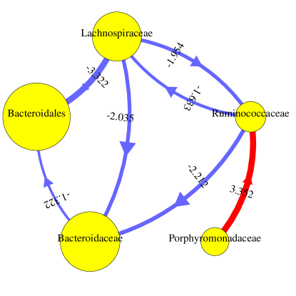
Figure 1: Significant interactions between abundant families. Blue arrows represent negative interactions. Thickness of arrow is proportional to interaction strength. Radius of circle is proportional to growth rate.

We also compare the predictive performance of our approach and the least squares approach of the deterministic GLV model. We divide the data randomly into training and test data sets. We use a proportion $(1-1/k)$ of the data as the training set, and the remaining $1/k$ portion of the data as the test data. We consider $k=24,12$, and $8$. For each $k$, we average the results over 100 random splits. We report the one-step prediction errors obtained from both approaches in Table 3. The mean squared prediction error is defined as ${\textrm{mean~{}squared~{}prediction~{}error}}:=m^{-1}\sum^{m}_{i=1}(\hat{u}_{i}-u_{i})^{2},$ where $u_{i}$ is the observed value at $t_{i}$, $\hat{u}_{i}$ is computed from the training model based on the previous log-observed data point $u_{i-1}$ at time $t_{i-1}$. From the results, our method outperforms the deterministic GLV model approach in prediction. Although the purpose of the analysis is interpretation rather than prediction, improved predictive accuracy suggests a better fitting model, so the conclusions drawn are more likely to be accurate.

Table 3: Cross-validated mean squared prediction error (standard error) of one-step predictions on moving picture gut data, using a proportion $1/k$ of the data as test data, averaged over 100 training-test splits. ‘GLV’ is the deterministic GLV model method, and ‘SGLV’ is our method.

	mean squared prediction error (standard error)
$k$	$24$	$12$	$8$
$\rm GLV$	$1.346(0.105)$	$1.495(0.089)$	$1.762(0.096)$
$\rm SGLV$	$1.206(0.093)$	$1.410(0.083)$	$1.610(0.087)$

6 Conclusion

Motivated by analysis of microbiome data, we proposed a new SGLV model to study temporal dynamics of the microbiome, and derived a new set of general conditions to guarantee various mathematical properties including existence and uniqueness of a solution, the bounds of moments, stationarity and ergodicity. Further, we have developed an approximate maximum likelihood estimator for our model and established a theoretical guarantee for the consistency and asymptotic normality of our AMLE. We have demonstrated the efficiency of our methods using simulations and real microbiome data applications.

There are a number of important directions for future work. Firstly, we have assumed that the number of OTUs, $N$, is fixed. In many applications, $N$ can be much larger than the sample size, $n$, in which case, regularization methods are needed to ensure good estimation. Incorporating regularisation into our estimators is highly non-trivial because the penalized estimates of $A$ may not be non-positive definite. We may add additional constraints to guarantee non-positive definiteness of $A$. However, this may lead to challenges in both computation and theory, and therefore we leave this topic for future research. For the asymptotic consistency of our method, it is essential to assume that the time difference between consecutive samples converges to 0. When this assumption is violated, i.e. time difference between consecutive samples does not converge to 0, the finite sample properties of our AMLE are unclear, and it is an interesting problem to explore in the future.

Appendix A Additional Simulation Results

In this section, we present additional simulation results for various scenarios. In particular, we include simulation results with various sample sizes $n\in\{300,500,1000\}$, for Cases 1 and 2 from Section 4 in main paper. Time step sizes are still set at $\Delta_{i,t}\in\{0.1,0.3,0.5\}$ with probabilities $0.7$, $0.2$ and $0.1$ respectively. All results are based on 1,000 simulations, with mean square error results compared for the approximate maximum likelihood estimators of our SGLV model, and the least squares estimate under deterministic GLV Differential Equation.

Table S4: Simulation results for Case 1, $n=300$, based on 1000 simulations: mean squared errors (standard error) of estimates of $\{a_{kl},1\leq k\leq 5,1\leq l\leq 5\}$ and $\{r_{k},1\leq k\leq 5\}$.

Method	Mean squared error (standard error)
	$a_{11}$	$a_{12}$	$a_{13}$	$a_{14}$	$a_{15}$	$r_{1}$	$\sigma^{2}_{1}$
GLV	$0.584(0.027)$	$1.271(0.057)$	$1.040(0.048)$	$3.305(0.144)$	$3.362(0.162)$	$0.332(0.016)$	$-$
SGLV	$0.442(0.021)$	$0.878(0.037)$	$0.720(0.031)$	$2.456(0.114)$	$2.329(0.105)$	$0.242(0.011)$	$0.765(3.590)\times 10^{-6}$
	$a_{21}$	$a_{22}$	$a_{23}$	$a_{24}$	$a_{25}$	$r_{2}$	$\sigma^{2}_{2}$
GLV	$0.483(0.021)$	$1.685(0.057)$	$1.291(0.049)$	$3.392(0.135)$	$2.500(0.115)$	$0.343(0.015)$	$-$
SGLV	$0.430(0.019)$	$1.093(0.042)$	$0.952(0.038)$	$2.566(0.110)$	$2.124(0.098)$	$0.272(0.012)$	$4.189(3.163)\times 10^{-6}$
	$a_{31}$	$a_{32}$	$a_{33}$	$a_{34}$	$a_{35}$	$r_{3}$	$\sigma^{2}_{3}$
GLV	$0.485(0.020)$	$1.272(0.051)$	$1.412(0.047)$	$2.050(0.089)$	$2.350(0.106)$	$0.426(0.016)$	$-$
SGLV	$0.424(0.018)$	$0.989(0.041)$	$0.871(0.033)$	$1.937(0.086)$	$2.182(0.099)$	$0.305(0.012)$	$4.757(3.327)\times 10^{-6}$
	$a_{41}$	$a_{42}$	$a_{43}$	$a_{44}$	$a_{45}$	$r_{4}$	$\sigma^{2}_{4}$
GLV	$0.493(0.019)$	$0.817(0.039)$	$0.579(0.027)$	$5.111(0.167)$	$2.131(0.099)$	$0.245(0.010)$	$-$
SGLV	$0.418(0.018)$	$0.718(0.033)$	$0.548(0.027)$	$3.029(0.114)$	$1.947(0.089)$	$0.212(0.010)$	$5.602(3.896)\times 10^{-6}$
	$a_{51}$	$a_{52}$	$a_{53}$	$a_{54}$	$a_{55}$	$r_{5}$	$\sigma^{2}_{5}$
GLV	$0.555(0.023)$	$1.274(0.053)$	$1.285(0.048)$	$3.289(0.134)$	$3.299(0.120)$	$0.408(0.015)$	$-$
SGLV	$0.454(0.021)$	$0.942(0.040)$	$0.930(0.036)$	$2.523(0.106)$	$2.221(0.095)$	$0.291(0.012)$	$3.361(2.945)\times 10^{-6}$

Table S5: Simulation results for Case 1, $n=500$ based on 1000 simulations: mean squared errors (standard error) of estimates of $\{a_{kl},1\leq k\leq 5,1\leq l\leq 5\}$ and $\{r_{k},1\leq k\leq 5\}$.

Method	Mean squared error(standard error)
	$a_{11}$	$a_{12}$	$a_{13}$	$a_{14}$	$a_{15}$	$r_{1}$	$\sigma^{2}_{1}$
GLV	$0.361(0.016)$	$0.978(0.043)$	$0.733(0.030)$	$2.214(0.100)$	$1.805(0.082)$	$0.221(0.010)$	$-$
SGLV	$0.279(0.013)$	$0.672(0.028)$	$0.498(0.021)$	$1.715(0.073)$	$1.358(0.063)$	$0.162(0.007)$	$0.467(3.402)\times 10^{-6}$
	$a_{21}$	$a_{22}$	$a_{23}$	$a_{24}$	$a_{25}$	$r_{2}$	$\sigma^{2}_{2}$
GLV	$0.279(0.012)$	$1.781(0.050)$	$1.027(0.035)$	$2.682(0.100)$	$1.521(0.066)$	$0.270(0.011)$	$-$
SGLV	$0.243(0.011)$	$1.005(0.032)$	$0.688(0.025)$	$1.954(0.077)$	$1.288(0.058)$	$0.184(0.007)$	$3.640(2.586)\times 10^{-6}$
	$a_{31}$	$a_{32}$	$a_{33}$	$a_{34}$	$a_{35}$	$r_{3}$	$\sigma^{2}_{3}$
GLV	$0.308(0.014)$	$1.076(0.037)$	$1.452(0.042)$	$1.501(0.065)$	$1.520(0.066)$	$0.355(0.012)$	$-$
SGLV	$0.261(0.011)$	$0.779(0.029)$	$0.852(0.028)$	$1.174(0.054)$	$1.397(0.062)$	$0.239(0.009)$	$4.497(2.950)\times 10^{-6}$
	$a_{41}$	$a_{42}$	$a_{43}$	$a_{44}$	$a_{45}$	$r_{4}$	$\sigma^{2}_{4}$
GLV	$0.355(0.013)$	$0.528(0.025)$	$0.310(0.013)$	$5.643(0.140)$	$1.080(0.047)$	$0.170(0.007)$	$-$
SGLV	$0.267(0.011)$	$0.450(0.021)$	$0.292(0.013)$	$3.164(0.098)$	$0.901(0.041)$	$0.135(0.006)$	$5.274(3.457)\times 10^{-6}$
	$a_{51}$	$a_{52}$	$a_{53}$	$a_{54}$	$a_{55}$	$r_{5}$	$\sigma^{2}_{5}$
GLV	$0.349(0.014)$	$0.995(0.037)$	$0.970(0.035)$	$2.148(0.088)$	$2.821(0.101)$	$0.320(0.011)$	$-$
SGLV	$0.268(0.011)$	$0.700(0.028)$	$0.676(0.025)$	$1.604(0.068)$	$1.832(0.071)$	$0.217(0.008)$	$2.995(2.540)\times 10^{-6}$

Table S6: Simulation results for Case 2, $n=300$ based on 1000 simulations: mean squared errors (standard error) of estimates of $\{a_{kl},1\leq k\leq 5,1\leq l\leq 5\}$ and $\{r_{k},1\leq k\leq 5\}$.

Method	Mean squared error (standard error)
	$a_{11}$	$a_{12}$	$a_{13}$	$a_{14}$	$a_{15}$	$r_{1}$	$\sigma^{2}_{1}$
GLV	$6.939(0.592)$	$2.890(0.137)$	$1.432(0.064)$	$5.648(0.282)$	$4.817(0.216)$	$0.695(0.026)$	$-$
SGLV	$6.221(0.455)$	$2.153(0.104)$	$1.055(0.048)$	$4.327(0.205)$	$3.793(0.175)$	$0.233(0.011)$	$0.007(0.022)$
	$a_{21}$	$a_{22}$	$a_{23}$	$a_{24}$	$a_{25}$	$r_{2}$	$\sigma^{2}_{2}$
GLV	$3.811(0.290)$	$2.488(0.105)$	$1.632(0.066)$	$4.949(0.211)$	$4.441(0.266)$	$0.744(0.024)$	$-$
SGLV	$3.481(0.251)$	$2.002(0.100)$	$1.239(0.050)$	$3.921(0.170)$	$3.618(0.220)$	$0.234(0.011)$	$0.021(0.023)$
	$a_{31}$	$a_{32}$	$a_{33}$	$a_{34}$	$a_{35}$	$r_{3}$	$\sigma^{2}_{3}$
GLV	$3.692(0.223)$	$2.671(0.117)$	$1.501(0.055)$	$3.878(0.198)$	$3.808(0.185)$	$0.838(0.024)$	$-$
SGLV	$3.059(0.186)$	$2.060(0.092)$	$1.018(0.043)$	$3.123(0.148)$	$3.271(0.156)$	$0.253(0.010)$	$0.035(0.030)$
	$a_{41}$	$a_{42}$	$a_{43}$	$a_{44}$	$a_{45}$	$r_{4}$	$\sigma^{2}_{4}$
GLV	$3.969(0.272)$	$1.866(0.090)$	$0.876(0.041)$	$5.498(0.212)$	$3.759(0.198)$	$0.502(0.017)$	$-$
SGLV	$3.205(0.223)$	$1.715(0.084)$	$0.792(0.037)$	$3.949(0.168)$	$3.456(0.173)$	$0.170(0.008)$	$0.033(0.028)$
	$a_{51}$	$a_{52}$	$a_{53}$	$a_{54}$	$a_{55}$	$r_{5}$	$\sigma^{2}_{5}$
GLV	$4.442(0.316)$	$2.310(0.112)$	$1.546(0.067)$	$4.705(0.211)$	$4.723(0.199)$	$0.802(0.025)$	$-$
SGLV	$3.376(0.216)$	$1.874(0.092)$	$1.123(0.049)$	$3.645(0.164)$	$3.784(0.192)$	$0.239(0.010)$	$0.023(0.021)$

Table S7: Simulation results for Case 2, $n=500$ based on 1000 simulations: mean squared error(standard error) of estimates of $\{a_{kl},1\leq k\leq 5,1\leq l\leq 5\}$ and $\{r_{k},1\leq k\leq 5\}$.

Method	mean squared error(standard error)
	$a_{11}$	$a_{12}$	$a_{13}$	$a_{14}$	$a_{15}$	$r_{1}$	$\sigma^{2}_{1}$
GLV	$6.166(0.677)$	$1.840(0.082)$	$1.049(0.044)$	$3.157(0.144)$	$2.690(0.117)$	$0.596(0.018)$	$-$
SGLV	$5.556(0.509)$	$1.377(0.059)$	$0.697(0.031)$	$2.380(0.112)$	$2.028(0.091)$	$0.140(0.006)$	$0.004(0.020)$
	$a_{21}$	$a_{22}$	$a_{23}$	$a_{24}$	$a_{25}$	$r_{2}$	$\sigma^{2}_{2}$
GLV	$3.196(0.222)$	$1.768(0.065)$	$1.056(0.041)$	$3.523(0.151)$	$2.526(0.114)$	$0.613(0.017)$	$-$
SGLV	$2.714(0.181)$	$1.208(0.049)$	$0.716(0.030)$	$2.523(0.115)$	$2.024(0.094)$	$0.140(0.006)$	$0.017(0.017)$
	$a_{31}$	$a_{32}$	$a_{33}$	$a_{34}$	$a_{35}$	$r_{3}$	$\sigma^{2}_{3}$
GLV	$3.517(0.236)$	$1.706(0.069)$	$1.546(0.045)$	$2.111(0.105)$	$2.172(0.099)$	$0.874(0.019)$	$-$
SGLV	$2.921(0.195)$	$1.274(0.054)$	$0.950(0.031)$	$1.879(0.089)$	$1.817(0.081)$	$0.223(0.008)$	$0.030(0.023)$
	$a_{41}$	$a_{42}$	$a_{43}$	$a_{44}$	$a_{45}$	$r_{4}$	$\sigma^{2}_{4}$
GLV	$3.196(0.211)$	$1.055(0.052)$	$0.468(0.022)$	$4.900(0.156)$	$2.072(0.108)$	$0.456(0.013)$	$-$
SGLV	$2.871(0.207)$	$0.953(0.047)$	$0.417(0.018)$	$3.028(0.108)$	$1.856(0.100)$	$0.114(0.005)$	$0.029(0.022)$
	$a_{51}$	$a_{52}$	$a_{53}$	$a_{54}$	$a_{55}$	$r_{5}$	$\sigma^{2}_{5}$
GLV	$3.381(0.259)$	$1.750(0.073)$	$1.168(0.043)$	$2.951(0.126)$	$3.916(0.134)$	$0.835(0.020)$	$-$
SGLV	$2.662(0.194)$	$1.314(0.057)$	$0.859(0.035)$	$2.374(0.103)$	$2.585(0.102)$	$0.201(0.008)$	$0.021(0.019)$

Table S8: Simulation results for Case 2, $n=1000$ based on 1000 simulations: mean squared errors (standard error) of estimates of $\{a_{kl},1\leq k\leq 5,1\leq l\leq 5\}$ and $\{r_{k},1\leq k\leq 5\}$.

Method	Mean squared errors (standard error)
	$a_{11}$	$a_{12}$	$a_{13}$	$a_{14}$	$a_{15}$	$r_{1}$	$\sigma^{2}_{1}$
GLV	$5.817(0.714)$	$1.038(0.044)$	$0.657(0.027)$	$1.524(0.071)$	$1.215(0.059)$	$0.508(0.013)$	$-$
SGLV	$4.634(0.431)$	$0.735(0.033)$	$0.445(0.019)$	$1.083(0.050)$	$0.941(0.045)$	$0.077(0.003)$	$0.002(0.018)$
	$a_{21}$	$a_{22}$	$a_{23}$	$a_{24}$	$a_{25}$	$r_{2}$	$\sigma^{2}_{2}$
GLV	$3.279(0.360)$	$1.684(0.050)$	$0.721(0.023)$	$2.109(0.074)$	$1.162(0.054)$	$0.598(0.011)$	$-$
SGLV	$2.631(0.183)$	$1.020(0.039)$	$0.493(0.034)$	$1.480(0.047)$	$0.895(0.046)$	$0.098(0.012)$	$0.013(0.014)$
	$a_{31}$	$a_{32}$	$a_{33}$	$a_{34}$	$a_{35}$	$r_{3}$	$\sigma^{2}_{3}$
GLV	$2.618(0.183)$	$1.080(0.039)$	$1.552(0.034)$	$1.082(0.047)$	$1.073(0.046)$	$0.831(0.012)$	$-$
SGLV	$2.254(0.162)$	$0.755(0.030)$	$0.914(0.023)$	$0.902(0.040)$	$0.892(0.040)$	$0.178(0.005)$	$0.029(0.019)$
	$a_{41}$	$a_{42}$	$a_{43}$	$a_{44}$	$a_{45}$	$r_{4}$	$\sigma^{2}_{4}$
GLV	$2.737(0.231)$	$0.513(0.025)$	$0.232(0.010)$	$4.988(0.119)$	$0.928(0.43)$	$0.465(0.009)$	$-$
SGLV	$2.383(0.199)$	$0.458(0.022)$	$0.193(0.009)$	$2.900(0.082)$	$0.781(0.036)$	$0.074(0.003)$	$0.027(0.019)$
	$a_{51}$	$a_{52}$	$a_{53}$	$a_{54}$	$a_{55}$	$r_{5}$	$\sigma^{2}_{5}$
GLV	$3.071(0.203)$	$1.045(0.040)$	$0.809(0.025)$	$1.740(0.072)$	$3.574(0.099)$	$0.799(0.013)$	$-$
SGLV	$2.583(0.191)$	$0.771(0.31)$	$0.549(0.018)$	$1.299(0.056)$	$2.166(0.070)$	$0.161(0.005)$	$0.018(0.014)$

Table S9: 5% Confidence intervals for estimated interaction coefficients for the five most abundant families in person 2^′s gut using our approach. The significantly non-zero interaction coefficients are highlighted in blue (for negative values).

	B.	R.	L.	P.	B′.
Bacteroidaceae	$(-2.575,-1.420)$	$\pagecolor{blue!30!white!70}{(-3.677,-0.747)}$	$\pagecolor{blue!30!white!70}{(-3.842,-0.228)}$	$(-0.143,5.568)$	$(-4.361,4.713)$
Ruminococcaceae	$(-0.338,0.354)$	$(-4.836,-3.079)$	$(-3.037,-0.871)$	$\pagecolor{red!30!white!70}{(1.641,5.063)}$	$(-3.321,2.118)$
Lachnospiraceae	$(-0.884,0.155)$	$\pagecolor{blue!30!white!70}{(-2.951,-0.314)}$	$(-7.107,-3.854)$	$(-1.511,3.628)$	$(-4.688,3.479)$
Porphyromonadaceae	$(-0.742,0.125)$	$(-1.064,1.136)$	$(-1.140,1.374)$	$(-12.515,-8.228)$	$(-2.996,3.817)$
Bacteroidales (unsp.)	$\pagecolor{blue!30!white!70}{(-1.959,-0.686)}$	$(-3.199,0.030)$	$\pagecolor{blue!30!white!70}{(-5.313,-1.330)}$	$(-1.131,5.162)$	$(-13.984,-3.983)$

Table S10: Estimated growth rates, interaction coefficients and diffusion coefficients for the five most abundant families in Person 2’s gut under the deterministic GLV model. The significantly non-zero interaction coefficients (at the 5% significance level) are highlighted in blue.

	B.	R.	L.	P.	B′.	$r_{i}$	$\sigma^{2}_{i}$
Bacteroidaceae	$-1.130$	$-0.406$	$-0.902$	$1.875$	$1.174$	0.497	-
Ruminococcaceae	$0.042$	$-3.068$	$-1.198$	$1.207$	$-0.081$	0.510	-
Lachnospiraceae	$-0.018$	$-0.930$	$-3.946$	$-1.021$	$-0.223$	0.703	-
Porphyromonadaceae	$-0.225$	$-0.057$	$-0.328$	$-8.630$	$0.281$	0.572	-
Bacteroidales (unsp.)	$-0.456$	$0.127$	$-2.090$	$1.431$	$-8.072$	0.659	-

Table S11: Bootstrap 5% Confidence intervals for deterministic GLV model estimates of interaction coefficients and growth rates for the five most abundant families in Person 2’s gut. The significantly non-zero inter-species interaction coefficients are highlighted in blue.

	B.	R.	L.	P.	B′.
Bacteroidaceae	$(-2.614,-0.707)$	$(-3.941,1.087)$	$(-4.775,0.987)$	$(-6.062,9.060)$	$(-3.013,4.297)$
Ruminococcaceae	$(-0.597,0.707)$	$(-5.068,-2.105)$	$(-3.138,-0.056)$	$(-2.540,5.628)$	$(-3.972,2.684)$
Lachnospiraceae	$(-0.914,0.426)$	$(-3.713,0.343)$	$(-7.329,-2.343)$	$(-6.414,4.292)$	$(-3.378,2.603)$
Porphyromonadaceae	$(-0.830,0.461)$	$(-1.324,2.109)$	$(-3.172,2.311)$	$(-12.779,-5.178)$	$(-4.429,4.612)$
Bacteroidales (unsp.)	$(-2.064,-0.022)$	$(-3.579,1.602)$	$(-5.997,0.006)$	$(-6.647,8.029)$	$(-13.143,-4.039)$

Figure S2: (a) Relative abundance of the family Bacteroidaceae over time; (b) Logarithm of the temporal data in (a) and the fitting curve (blue line) from the SGLV model.

(a) Proportion

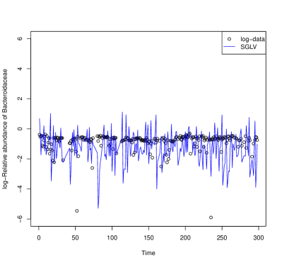
(b) log-proportion with one-step predictions (in blue)

Appendix B Proof of Propositions

We first show the existence and uniqueness of solutions to our stochastic differential equation model (3). We first recall the assumptions needed:

Assumption 1.

The initial value $x(0)=(x_{1}(0),\ldots,x_{N}(0))^{{\mathrm{\scriptscriptstyle T}}}\in\mathbb{R}^{N}_{+}$, $r_{k}-\sigma^{2}_{k}/2>0,\sigma_{k}>0$, and $A=(a_{kl})_{N\times N}$ is non-positive definite.

Assumption 2.

For some $\phi\geq 4$, the elements of $A$ satisfy $a_{kk}+\phi(\phi+1)^{-1}\sum_{l=1}^{N}(a_{kl}\lor 0)+(\phi+1)^{-1}\sum_{l=1}^{N}(a_{lk}\lor 0)<0.$

Assumption 3.

Each element of the vector $\tilde{x}=(\tilde{x}_{1},...,\tilde{x}_{N})^{{\mathrm{\scriptscriptstyle T}}}=-A^{-1}\left(r-\sigma^{2}/2\right)$ is positive, i.e., $\tilde{x}_{k}>0$ for $k=1,...,N$.

Assumption 4.

There exist positive constants $c_{1}$,$\ldots$, $c_{N}$ such that for $k=1,...,N$,

$$\sum^{N}_{i=1}c_{i}\sigma^{2}_{i}\tilde{x}_{i}<-\left[2c_{k}a_{kk}+\sum_{l\neq k}\{c_{k}|a_{kl}|+c_{l}|a_{lk}|\}\right]\tilde{x}^{2}_{k}.$$

Proposition 1.

For $t\geq 0$, under Assumption 1, there is a unique solution $x(t)$ to SGLV model (3) and $x(t)\in\mathbb{R}^{N}_{+}$ almost surely.

Proof.

Since the coefficients of the equation are locally Lipschitz continuous, for any given initial value $x(0)\in\mathbb{R}_{+}$ there is a unique local solution $x(t)$ on $t\in[0,\tau_{e})$, where $\tau_{e}$ is the explosion time. To show that the solution is global, it is equivalent to show that $\tau_{e}=+\infty$ a.s. Define a $C^{2}$-function $V:\mathbb{R}^{N}_{+}\rightarrow\mathbb{R}_{\geq 0}$ by

$$V(x(t)) = \sum^{N}_{k=1}\{x_{k}(t)-1-\log(x_{k}(t))\}.$$

Note that $V(x(t))$ is non-negative because $x_{k}(t)-1-\log(x_{k}(t))\geq 0$ for all $x_{k}(t)>0,k=1,...,N$. Furthermore, $V(x(t))\rightarrow\infty$ for any explosion time of $x(t)$, so $\tau_{e}$ is the explosion time of $V(x(t))$.

We choose a sufficiently large non-negative number $\eta_{0}$ such that $V(x(0))\leq\eta_{0}$. For each $\eta\geq\eta_{0}$, we can define the stopping time

$$\tau_{\eta} = \inf\{t\in[0,\tau_{e})|V(x(t))\geq\eta\}$$

Clearly, $\tau_{\eta}$ is increasing. Set $\tau_{\infty}=\lim_{\eta\rightarrow\infty}\tau_{\eta}$. Since $\tau_{\infty}\leq\tau_{e}$, it is sufficient to prove $\tau_{\infty}=\infty$ a.s. This is equivalent to showing for any $T<\infty$ that $P(\tau_{\eta}\leq T)\rightarrow 0$ as $\eta\rightarrow\infty$.

By Itô’s formula, we get

$$\mathrm{d}V(x(t)) = F_{1}(x(t))dt+\sum^{N}_{k=1}\sigma_{k}\{x_{k}(t)-1\}dB_{k}(t),$$ (S10)

where

$$F_{1}(x(t)) := \sum^{N}_{k=1}\{r_{k}x_{k}(t)-(r_{k}-\sigma^{2}_{k}/2)\}+\sum^{N}_{k=1}\{x_{k}(t)-1\}\sum^{N}_{l=1}a_{kl}x_{l}(t).$$

Because $A$ is a non-positive definite matrix, $\sum^{N}_{k=1}\sum^{N}_{l=1}a_{kl}x_{k}(t)x_{l}(t)\leq 0$ and we have

$$F_{1}(x(t)) \leq \sum^{N}_{k=1}r_{k}x_{k}(t)-\sum^{N}_{k,l=1}a_{kl}x_{l}(t)-\sum^{N}_{k=1}(r_{k}-\sigma^{2}_{k}/2)$$

$$\leq C\sum^{N}_{k=1}x_{k}(t)+NC,$$

where $C=\max_{k=1,...,N}\{(r_{k}-\sum^{N}_{l=1}a_{lk})\vee(r_{k}-\sigma^{2}_{k}/2)\vee 0\}$. From the inequality $x_{k}(t)\leq 2\{x_{k}(t)-1-\log(x_{k}(t))\}+2$, we have

$$F_{1}(x(t))\leq 2CV(x(t))+3NC,$$

so, from Equation (S10)

$$\mathrm{d}V(x(t)) \leq \{2CV(x(t))+3NC\}dt+\sum^{N}_{k=1}\sigma_{k}\{x_{k}(t)-1\}dB_{k}(t),$$

and

$$\int^{T\wedge\tau_{\eta}}_{0}dV(x(t))\leq\int^{T\wedge\tau_{\eta}}_{0}\{2CV(x(t))+3NC\}dt+\int^{T\wedge\tau_{\eta}}_{0}\sum^{N}_{k=1}\sigma_{k}\{x_{k}(t)-1\}dB_{k}(t).$$

Taking expectations on both sides,

$$E\{V(x(T\wedge\tau_{\eta}))\} \leq V(x(0))+2CE\left\{\int^{T\wedge\tau_{\eta}}_{0}V(x(t))dt\right\}+3NCE(T\wedge\tau_{\eta})$$

$$\leq V(x(0))+3NCT+2CE\left\{\int^{T\wedge\tau_{\eta}}_{0}V(x(t))dt\right\}.$$

By Grönwall’s inequality, we have

$$E\{V(x(T\wedge\tau_{\eta}))\} \leq \{V(x(0))+3NCT\}\exp(2CT).$$

By definition of $\tau_{\eta}$, we have $V(x(\tau_{\eta}))=\eta$, so

$$\{V(x(0))+3NCT\}\exp(2CT)\geq E\{V(x(T\land\tau_{\eta}))\}\geq\eta P(\tau_{\eta}\leq T).$$

The left side of this inequality is bounded, so we must have $P(\tau_{\eta}\leq T)\rightarrow 0$ as $\eta\rightarrow\infty$. ∎

Proposition 2.

Under Assumptions 1 and 2, there exist positive constants $C_{1}$ and $C_{2}$ such that for any initial value $x_{0}\in\mathbb{R}_{+}^{N}$, the solution of SGLV model (3) has the properties

$$\limsup_{t\rightarrow+\infty}\sum^{N}_{k=1}E\{x^{\theta}_{k}(t)\}\leq C_{1},\quad\limsup_{t\rightarrow+\infty}\sum^{N}_{k=1}t^{-1}E\left\{\int^{t}_{0}x^{\%theta}_{k}(s)ds\right\}\leq C_{2},$$

for any $0\leqslant\theta\leq 4$.

Proof.

Since the existence of higher moments implies the existence of lower moments, it is sufficient to prove the results for some $\theta\geqslant 4$. We show that the result holds for $\theta=\phi$ from Assumption 2. Define a $C^{2}$-function $V:\mathbb{R}^{N}_{+}\rightarrow\mathbb{R}_{+}$ by $V(x(t))=\sum^{N}_{k=1}x^{\phi}_{k}(t)$, where $x(t)=(x_{1}(t),...,x_{N}(t))^{{\mathrm{\scriptscriptstyle T}}}$. We apply Itô’s formula to $e^{t}V(x(t))$ and get

$$\mathrm{d}\{e^{t}V(x(t))\}=e^{t}F(x(t))\mathrm{d}t+e^{t}\sum^{N}_{k=1}\phi\sigma_{k}x^{\phi}_{k}(t)\mathrm{d}B_{k}(t),$$

where

$$F(x(t)):=V(x(t))+\phi\sum^{N}_{k=1}r_{k}x^{\phi}_{k}(t)+\phi\sum^{N}_{k,l=1}a_{kl}x^{\phi}_{k}(t)x_{l}(t)+\{\phi(\phi-1)/2\}\sum^{N}_{k=1}\sigma^{2}_{k}x^{\phi}_{k}(t).$$ (S11)

Note that, setting $J_{k}=\{l\neq k|a_{kl}<0\}$, we have

$$\sum^{N}_{k,l=1}a_{kl}x^{\phi}_{k}(t)x_{l}(t) = \sum^{N}_{k=1}a_{kk}x^{\phi+1}_{k}(t)+\sum^{N}_{k=1}\left(\sum_{l\in J_{k}}+\sum_{l\in J^{c}_{k}}\right)a_{kl}x^{\phi}_{k}(t)x_{l}(t)$$

$$\leq \sum^{N}_{k=1}a_{kk}x^{\phi+1}_{k}(t)+\sum^{N}_{k=1}\sum_{l\in J^{c}_{k}}a_{kl}x^{\phi}_{k}(t)x_{l}(t)$$

$$\leq \sum^{N}_{k=1}a_{kk}x^{\phi+1}_{k}(t)+\sum^{N}_{k=1}\sum_{l\in J^{c}_{k}}a_{kl}\left\{\phi(\phi+1)^{-1}x^{\phi+1}_{k}(t)+(\phi+1)^{-1}x^{\phi+1}_{l}(t)\right\}$$

$$= \sum^{N}_{k=1}x^{\phi+1}_{k}(t)\left\{a_{kk}+\phi(\phi+1)^{-1}\sum^{N}_{l=1}(a_{kl}\vee 0)+(\phi+1)^{-1}\sum^{N}_{l=1}(a_{lk}\vee 0)\right\}.$$

Since $a_{kk}+\phi(\phi+1)^{-1}\sum^{N}_{l=1}(a_{kl}\vee 0)+(\phi+1)^{-1}\sum^{N}_{l=1}(a_{lk}\vee 0)<0$, $F(x(t))$ is bounded. Let $C_{1}:=\sup_{x(t)\in\mathbb{R}^{N}_{+}}F(x(t))<+\infty$, and we have

$$\mathrm{d}\{\exp(t)V(x(t))\}\leq C_{1}\exp(t)\mathrm{d}t+\exp(t)\sum^{N}_{k=1}\phi\sigma_{k}x^{\phi}_{k}(t)\mathrm{d}B_{k}(t).$$ (S12)

Let $\eta_{0}>V(x(0))$. For each $\eta\geq\eta_{0}$, we define the stopping time

$$\tau_{\eta}=\inf\{t\geq 0|V(x(t))\geq\eta\}.$$

It then follows from Equation (S12)

$$E\left[\int^{t\wedge\tau_{\eta}}_{0}d\{\exp(s)V(x(s))\}\right]\leq E\left[\int^{t\wedge\tau_{\eta}}_{0}C_{1}\exp(s)ds\right]+E\left[\int^{t\wedge\tau_{\eta}}_{0}\exp(s)\sum^{N}_{k=1}\phi\sigma_{k}x^{\phi}_{k}(s)dB_{k}(s)\right],$$

where $\int^{t\wedge\tau_{\eta}}_{0}\exp(s)\sum^{N}_{k=1}\phi\sigma_{k}x^{\phi}_{k}(s)dB_{k}(s)$ is a martingale with expectation equal to zero, so we have

$$E\{\exp(t\wedge\tau_{\eta})V(x(t\wedge\tau_{\eta}))\}\leq V(x_{0})+C_{1}E\left(\int^{t\wedge\tau_{\eta}}_{0}\exp(s)ds\right).$$

By the proof of Proposition 1, $\tau_{\eta}\rightarrow\infty$ almost surely as $\eta\rightarrow+\infty$. So we have

$$\exp(t)E\{V(x(t))\}\leq V(x_{0})+C_{1}(\exp(t)-1),$$ (S13)

thus

$$\limsup_{t\rightarrow+\infty}\sum^{N}_{k=1}E\{x^{\phi}_{k}(t)\} \leq C_{1}.$$

Integrating both sides of equation (S13) divided by $\exp(t)$, we can get

$$\limsup_{t\rightarrow+\infty}t^{-1}\int^{t}_{0}E\{V(x(s))\}ds \leq C_{2}.$$

By Fubini’s theorem, we obtain the result. ∎

The proof of Proposition 3, uses the following theorems from Chapter 4 of Kaśminskii (2011).

Theorem 4.1 (Stationarity).

If Assumptions B.1–B.2 hold, then the Markov process $X(t)$ has a unique stationary distribution $\mu(\cdot)$.

Theorem 4.2 (Ergodicity).

Suppose that Assumptions B.1–B.2 hold, and let $\mu$ be the stationary distribution of the process $X(t)$. Let $f(\cdot)$ be a function integrable with respect to the measure $\mu$. Then

$$P_{x}\left\{\lim_{T\rightarrow+\infty}\frac{1}{T}\int^{T}_{0}f(X(t))dt=\int_{\mathbb{R}^{N}}f(x)\mu(dx)\right\} = 1$$ (S14)

for all $x\in\mathbb{R}^{N}$.

The Assumptions B.1–B.2 are as follows: There exists a bounded open domain $U\subset\mathbb{R}^{N}$ with regular boundary $\Gamma$, having the following properties:

Assumption B.1.

In the domain $U$ and some neighborhood thereof, the smallest eigenvalue of the diffusion matrix $\Sigma(x)$ is bounded away from zero.

Assumption B.2.

If $x\in\mathbb{R}^{N}\setminus U$, the mean time $\tau$ at which a path issuing from $x$ reaches the set $U$ is finite, and $\sup_{x\in K}E_{x}\tau<\infty$ for every compact subset $K\subset\mathbb{R}^{N}$.

Proposition 3.

Under Assumptions 1, 3 and 4, there is a stationary distribution for the solution of SGLV model (3), and it has the ergodic property.

Proof.

To apply Theorems 4.1 and 4.2, we first need to show that Assumptions B.1–B.2 hold. For Assumption B.1, Since $\sigma_{k}>0$ in SGLV (3), the smallest eigenvalue of the diffusion matrix $\Sigma={\rm diag}(\sigma^{2}_{1},...,\sigma^{2}_{N})$ is bounded away from zero. To verify Assumption B.2, it is sufficient to show that there exists some neighborhood $U$ and a non-negative $C^{2}$-function $V(x(t))$ such that and for any $x(t)\in\mathbb{R}^{N}\setminus U$, $\mathcal{L}V$ is negative (for details, refer to Zhu & Yin (2007)), where

$$\mathcal{L}:=\sum^{N}_{k=1}x_{k}(t)\left\{r_{k}+\sum^{N}_{l=1}a_{kl}x_{l}(t)\right\}\partial(\cdot)\{\partial x_{k}(t)\}^{-1}+2^{-1}\sum^{N}_{k=1}\sigma^{2}_{k}\partial^{2}(\cdot)\{\partial x_{k}(t)\partial x_{l}(t)\}^{-1}.$$ (S15)

By Assumption 3 , $\tilde{x}=(\tilde{x}_{1},...,\tilde{x}_{N})^{{\mathrm{\scriptscriptstyle T}}}$ is positive. We define a non-negative $C^{2}-$function $V^{\ast}(x(t))=\sum^{N}_{k=1}c_{k}\{x_{k}(t)-\tilde{x}_{k}-\tilde{x}_{k}\log(x_{k}(t)/\tilde{x}_{k})\}$ and will show that there exists a constant $C^{\ast}>0$ such that

$$\mathcal{L}V^{\ast}(x(t))\leq-C^{\ast},$$

where $\mathcal{L}$, defined by Equation (S15), denotes the infinitesimal generator of stochastic differential equation (3). It is easy to see that $V^{\ast}(x(t))\rightarrow+\infty$ as $x(t)\rightarrow+\infty$ and $V^{\ast}(x(t))\rightarrow+\infty$ as $x(t)\rightarrow 0$. With some computation, we can get

$$\mathcal{L}V^{\ast}(x(t))$$

$$= \sum^{N}_{k=1}c_{k}a_{kk}\{x_{k}(t)-\tilde{x}_{k}\}^{2}+\sum^{N}_{k=1}\sum^{N}_{l\neq k}c_{k}a_{kl}\{x_{k}(t)-\tilde{x}_{k}\}\{x_{l}(t)-\tilde{x}_{l}\}+\frac{1}{2}\sum^{N}_{k=1}c_{k}\sigma^{2}_{k}\tilde{x}_{k}.$$

Note that

$$\sum^{N}_{k=1}\sum^{N}_{l\neq k}c_{k}a_{kl}\{x_{k}(t)-\tilde{x}_{k}\}\{x_{l}(t)-\tilde{x}_{l}\}$$

$$\leq \frac{1}{2}\sum^{N}_{k=1}\sum^{N}_{l\neq k}c_{k}|a_{kl}|\big{[}\{x_{k}(t)-\tilde{x}_{k}\}^{2}+\{x_{l}(t)-\tilde{x}_{l}\}^{2}\big{]},$$

so

$$\mathcal{L}V^{\ast}(x(t))\leq\frac{1}{2}\sum^{N}_{k=1}\left\{2c_{k}a_{kk}+\sum_{l\neq k}(c_{k}|a_{kl}|+c_{l}|a_{lk}|)\right\}\{x_{k}(t)-\tilde{x}_{k}\}^{2}+\frac{1}{2}\sum^{N}_{k=1}c_{k}\sigma^{2}_{k}\tilde{x}_{k}.$$

Assumption 4 gives that,

$$\sum^{N}_{k=1}c_{k}\sigma^{2}_{k}\tilde{x}_{k}<\min\left\{-\left\{2c_{k}a_{kk}+\sum_{l\neq k}(c_{k}|a_{kl}|+c_{l}|a_{lk}|)\right\}\tilde{x}^{2}_{k},k=1,...,N\right\}.$$

We consider the ellipsoid

$$\mathbb{E}=\left\{x(t)\middle|\sum^{N}_{k=1}\left\{2c_{k}a_{kk}+\sum_{l\neq k}(c_{k}|a_{kl}|+c_{l}|a_{lk}|)\right\}\left\{x_{k}(t)-\tilde{x}_{k}\right\}^{2}+\sum^{N}_{k=1}c_{k}\sigma^{2}_{k}\tilde{x}_{k}\geq 0\right\}.$$

It is easy to see that $\mathcal{L}V^{\ast}(x(t))>0$ in some subset of $\mathbb{E}$ (e.g.$\{x(t)=\tilde{x}(t)\}$)and $\mathcal{L}V^{\ast}(x(t))<0$ outside $\mathbb{E}$, so we can find a $\mathbb{D}\subseteq\mathbb{R}^{N}_{+}$ and a positive constant $C^{\ast}$, such that $\mathbb{D}\supset\mathbb{E}$ and $\mathcal{L}V^{\ast}(x(t))\leq-C^{\ast},~{}x(t)\in\mathbb{R}^{N}_{+}\setminus\bar{\mathbb{D}}$, where $\bar{\mathbb{D}}$ is the closure of $\mathbb{D}$, which implies the solution $x(t)$ is recurrent in the domain $\mathbb{D}$. By Theorem 4.1, $x(t)$ has a stationary distribution, and by the Theorem 4.2, it also has the ergodic property. ∎

Corollary 1.

Under Assumptions 1, 3 and 4, for any Borel measurable function $f(\cdot):\mathbb{R}^{N}_{+}\rightarrow\mathbb{R}$, which is integrable with respect to the density, $\pi(\cdot)$, of the stationary distribution, the solution of SGLV model (3) has the property,

$$\lim_{t\rightarrow+\infty}t^{-1}\int^{t}_{0}f(x(s))ds=\int_{\mathbb{R}^{N}_{+}}f(x)\pi(dx).$$

Proof.

By Proposition 3, there exists a stationary density for the stochastic differential equation, denoted by $\pi(\cdot)$. The ergodic theory on the stationary distribution (Theorem 4.2 from Kaśminskii (2011)) gives that for any Borel measurable function $f(\cdot):\mathbb{R}^{N}_{+}\rightarrow\mathbb{R}$, which is integrable with respect to $\pi(\cdot)$,

$$\lim_{t\rightarrow+\infty}t^{-1}\int^{t}_{0}f(x(s))ds=\int_{\mathbb{R}^{N}_{+}}f(x)\pi(dx),$$

holds with probability 1. ∎

Appendix C Proof of Theorems

Recall that the main theorems depend on the following additional assumptions:

Assumption 5.

$T$ is fixed, and $\Delta_{\max}\rightarrow 0$.

Assumption 6.

(I) $T\rightarrow+\infty$ and $\Delta_{\max}\rightarrow 0$; (II) $T\rightarrow+\infty$ and $T\Delta_{\max}\rightarrow 0$.

Before proving Theorem 1, we first prove the following key lemmas:

Lemma S1.

Suppose Assumptions 1, 2, and 5, hold. For fixed N and T, let $\Psi=\Theta\times\Phi$, and $\mathcal{K}\subset\Theta$ be a relatively compact set. Then for any $\tilde{\theta}=(\tilde{\vartheta},\sigma)\in\Psi$ , and $r=0,1,2$.

$$\sup_{\vartheta\in\overline{\mathcal{K}}}|(\partial/\partial\vartheta)^{r}\ell_{n,T}(\vartheta)-(\partial/\partial\vartheta)^{r}\ell_{T}(\vartheta)|=O_{P_{\tilde{\theta}}}(\Delta^{1/2}_{\max}),n\rightarrow+\infty,$$ (S16)

where $\overline{\mathcal{K}}$ is the closure of $\mathcal{K}$.

Proof.

Here we only consider the proof of the case $r=0$, because proofs of the cases $r=1$ and $r=2$ are similar to the case $r=0$. In order to show (S16), we only need to show that

$$\lim_{\kappa\rightarrow+\infty}P\left\{\sup_{\vartheta\in\overline{\mathcal{K}}}\big{|}\ell_{n,T}(\vartheta)-\ell_{T}(\vartheta)\big{|}>\kappa\Delta^{1/2}_{\max}\right\}\leq\lim_{\kappa\rightarrow+\infty}\kappa^{-1}\Delta^{-1/2}_{\max}E\left\{\sup_{\vartheta\in\overline{\mathcal{K}}}\big{|}\ell_{n,T}(\vartheta)-\ell_{T}(\vartheta)\big{|}\right\}=0.$$

We start by setting

$$\ell_{n,T}(\vartheta)-\ell_{T}(\vartheta) = \sum^{N}_{k=1}\sigma^{-2}_{k}\sum^{n-1}_{i=0}\int^{t_{i+1}}_{t_{i}}\left(\sum^{N}_{l=1}a_{kl}\{x_{l}(t_{i})-x_{l}(t)\}\right)\left\{\tilde{R}_{k}+\sum^{N}_{m=1}\tilde{a}_{km}x_{m}(t)\right\}dt$$

$$+\sum^{N}_{k=1}\sigma^{-1}_{k}\sum^{n-1}_{i=0}\int^{t_{i+1}}_{t_{i}}\sum^{N}_{l=1}a_{kl}\{x_{l}(t_{i})-x_{l}(t)\}dB_{k}(t)$$

$$-\sum^{N}_{k=1}2^{-1}\sigma^{-2}_{k}\sum^{n-1}_{i=0}\int^{t_{i+1}}_{t_{i}}\big{\{}R_{k}+\sum^{N}_{l}a_{kl}x_{l}(t_{i})\big{\}}^{2}-\big{\{}R_{k}+\sum^{N}_{l}a_{kl}x_{l}(t)\big{\}}^{2}dt$$

$$:= \mathrm{I}_{1}+\mathrm{I}_{2}+\mathrm{I}_{3},$$

where $\mathrm{I}_{1},\mathrm{I}_{2},\mathrm{I}_{3}$ are the three terms of the above equation. It is therefore sufficient to prove that for some constant $C$, we have $E\left(\sup_{\vartheta\in\overline{\mathcal{K}}}|\mathrm{I}_{i}|\right)<C\Delta_{\max}^{-1/2}$, for $i=1,2,3$.

$$E\sup_{\vartheta\in\bar{\mathcal{K}}}\mathrm{I}_{1} \leq \sum^{N}_{k=1}\sigma^{-2}_{k}\sum^{N}_{l=1}\left(\sup_{\vartheta\in\bar{\mathcal{K}}}|a_{kl}\tilde{R}_{k}|\right)\sum^{n-1}_{i=0}\int^{t_{i+1}}_{t_{i}}|\{x_{l}(t_{i})-x_{l}(t)\}|dt$$

$$+\sum^{N}_{k=1}\sum^{N}_{l,m=1}\sigma^{-2}_{k}\left(\sup_{\vartheta\in\bar{\mathcal{K}}}|a_{kl}\tilde{a}_{km}|\right)\sum^{n-1}_{i=0}\int^{t_{i+1}}_{t_{i}}|\{x_{l}(t_{i})-x_{l}(t)\}x_{m}(t)|dt,$$

$$E\sup_{\vartheta\in\bar{\mathcal{K}}}\mathrm{I}_{2} \leq \sum^{N}_{k=1}\sum^{N}_{l=1}\sigma^{-1}_{k}\left(\sup_{\vartheta\in\bar{\mathcal{K}}}|a_{kl}|\right)\sum^{n-1}_{i=0}E\left|\int^{t_{i+1}}_{t_{i}}\{x_{l}(t_{i})-x_{l}(t)\}dB_{k}(t)\right|$$

$$\leq \sum^{N}_{k=1}\sum^{N}_{l=1}\sigma^{-1}_{k}\left(\sup_{\vartheta\in\bar{\mathcal{K}}}|a_{kl}|\right)\sum^{n-1}_{i=0}\left(E\left[\int^{t_{i+1}}_{t_{i}}\{x_{l}(t_{i})-x_{l}(t)\}dB_{k}(t)\right]^{2}\right)^{1/2}$$

$$= \sum^{N}_{k=1}\sum^{N}_{l=1}\sigma^{-1}_{k}\left(\sup_{\vartheta\in\bar{\mathcal{K}}}|a_{kl}|\right)\sum^{n-1}_{i=0}\left(E\left[\int^{t_{i+1}}_{t_{i}}\{x_{l}(t_{i})-x_{l}(t)\}^{2}d(t)\right]\right)^{1/2},$$

$$E\sup_{\vartheta\in\bar{\mathcal{K}}}\mathrm{I}_{3} \leq \sum^{N}_{k=1}\sum^{N}_{l=1}\sigma^{-2}_{k}\left(\sup_{\vartheta\in\bar{\mathcal{K}}}|R_{k}a_{kl}|\right)\sum^{n-1}_{i=0}\int^{t_{i+1}}_{t_{i}}\left|\big{\{}x_{l}(t_{i})-x_{l}(t)\big{\}}\right|dt$$

$$+\sum^{N}_{k=1}\sum^{N}_{l,m=1}\sigma^{-2}_{k}\left(\sup_{\vartheta\in\bar{\mathcal{K}}}|R_{k}a_{kl}a_{km}|\right)\sum^{n-1}_{i=0}\int^{t_{i+1}}_{t_{i}}|\{x_{l}(t_{i})-x_{l}(t)\}\{x_{m}(t_{i})-x_{m}(t)\}|dt.$$

Since $\mathcal{K}$ is a relatively compact set, the terms, $\sup_{\vartheta\in\bar{\mathcal{K}}}|\tilde{R}_{k}a_{kl}|$, $\sup_{\vartheta\in\bar{\mathcal{K}}}|a_{kl}\tilde{a}_{km}|$, $\sup_{\vartheta\in\bar{\mathcal{K}}}|a_{kl}|$, $\sup_{\vartheta\in\bar{\mathcal{K}}}|R_{k}a_{kl}|$ and $\sup_{\vartheta\in\bar{\mathcal{K}}}|R_{k}a_{kl}a_{km}|$, are all bounded. By Itô’s isometry and Jensen’s inequality, we have

$$E\left|\int^{t_{i+1}}_{t_{i}}\{x_{l}(t_{i})-x_{l}(t)\}x_{m}(t)dt\right| \leq \int^{t_{i+1}}_{t_{i}}E|\{x_{l}(t_{i})-x_{l}(t)\}x_{m}(t)|dt,$$

and

$$\left[E\left|\int^{t_{i+1}}_{t_{i}}\!\!\!\big{\{}x_{l}(t_{i})-x_{l}(t)\}dB_{k}(t)\right|\right]^{2}$$

$$\leq E\left[\int^{t_{i+1}}_{t_{i}}\{x_{l}(t_{i})-x_{l}(t)\}dB_{k}(t)\right]^{2}$$

$$= \int^{t_{i+1}}_{t_{i}}E\left(\{x_{l}(t_{i})-x_{l}(t)\}^{2}\right)dt$$

$$= \int^{t_{i+1}}_{t_{i}}E[\{x_{l}(t_{i})-x_{l}(t)\}x_{l}(t_{i})]dt-\int^{t_{i+1}}_{t_{i}}E[\{x_{l}(t_{i})-x_{l}(t)\}x_{l}(t)]dt.$$

It is enough to show that there exist three constants $C$, $C_{1}$ and $C_{2}$ such that

$$E|\{x_{l}(t_{i})-x_{l}(t)\}x_{m}(t)| \leq C_{1}\Delta_{\max}+C_{2}\Delta^{1/2}_{\max},$$ (S17)

and

$$E\left(\{x_{l}(t_{i})-x_{l}(t)\}^{2}\right) \leq C\Delta_{i,t}.$$ (S18)

We prove (S17) using Proposition 2 and Itô’s isometry:

$$E|\{x_{l}(t)-x_{l}(t_{i})\}x_{m}(t)|$$ (S19)

$$= E\left|\int^{t}_{t_{i}}\left\{r_{k}+\sum^{N}_{l=1}a_{kl}x_{l}(s)\right\}x_{k}(s)x_{m}(t)ds+\int^{t}_{t_{i}}\sigma_{k}x_{k}(s)x_{m}(t)dB_{k}(s)\right|$$

$$\leq E\left|\int^{t}_{t_{i}}\left\{r_{k}+\sum^{N}_{l=1}a_{kl}x_{l}(s)\right\}x_{k}(s)x_{m}(t)ds\right|+E\left|\int^{t}_{t_{i}}\sigma_{k}x_{k}(s)x_{m}(t)dB_{k}(s)\right|$$

$$\leq E\bigg{|}\int^{t}_{t_{i}}\left\{r_{k}+\sum^{N}_{l=1}a_{kl}x_{l}(s)\right\}x_{k}(s)x_{m}(t)ds\bigg{|}+\sigma_{k}\left[E\left\{\int^{t}_{t_{i}}x^{2}_{m}(t)x^{2}_{k}(s)ds\right\}\right]^{1/2}$$

$$\leq C_{1}\Delta_{\max}+C_{2}\Delta^{1/2}_{\max}.$$

For (S18), we have:

$$E\left(\{x_{l}(t_{i})-x_{l}(t)\}^{2}\right) = E\left[\int^{t}_{t_{i}}\left\{r_{l}+\sum^{N}_{p=1}a_{lp}x_{p}(s)\right\}x_{l}(s)ds+\int^{t}_{t_{i}}\sigma_{l}dB_{l}(s)\right]^{2}$$

$$\leq 2\Delta_{i,t}E\left[\int^{t}_{t_{i}}\left\{r_{l}+\sum^{N}_{p=1}a_{lp}x_{p}(s)\right\}^{2}x^{2}_{l}(s)ds\right]+2\int^{t}_{t_{i}}\sigma^{2}_{l}E\{x^{2}_{l}(s)\}ds$$

$$\leq C\Delta_{i,t}.$$

Because $E\left(\sup_{\vartheta\in{\mathcal{K}}}|\mathrm{I}_{1}|\right)$, $E\left(\sup_{\vartheta\in{\mathcal{K}}}|\mathrm{I}_{2}|\right)$ and $E\left(\sup_{\vartheta\in{\mathcal{K}}}|\mathrm{I}_{3}|\right)$ are bounded by $C\Delta_{\max}^{-1/2}$ for some $C$, we have

$$P_{\tilde{\theta}}\left(\Delta^{-1/2}_{\max}\sup_{\vartheta\in\mathcal{K}}|\ell_{n,T}-\ell_{T}(\vartheta)|\geq\kappa\right)\leq C\kappa^{-1}$$

and

$$\lim_{\kappa\rightarrow+\infty}\limsup_{n}P_{\tilde{\theta}}\bigg{(}\Delta^{-1/2}_{\max}\sup_{\vartheta\in\Theta}\left|T^{-1}\ell_{n,T}(\vartheta)-T^{-1}\ell_{T}(\vartheta)\right|\geq\kappa\bigg{)} = 0.$$

∎

Theorem 1.

Under Assumptions 1, 2, and 5, we have that, conditional on the maximum likelihood estimators lying in some compact parameter space $\mathcal{K}$,

(i) $\|\hat{\vartheta}_{n,T}-\hat{\vartheta}_{T}\|=O_{p}\left(\Delta^{1/2}_{\max}\right)$.

(ii) For any $k\in\{1,...,N\}$, $(n/2)^{1/2}\sigma^{-2}_{k}(\widehat{\sigma}^{2}_{k,n,T}-\sigma^{2}_{k})\rightarrow N(0,1).$

Proof.

We Taylor expand $\ell^{\prime}_{T}(\hat{\vartheta}_{n,T})$ about $\hat{\vartheta}_{T}$. Because $\ell_{T}(\vartheta)$ is quadratic in $\vartheta$, the expansion is exact.

$$\ell^{\prime}_{T}(\hat{\vartheta}_{n,T}) = \ell^{\prime}_{T}(\hat{\vartheta}_{T})+\ell^{\prime\prime}_{T}(\hat{\vartheta}_{T})(\hat{\vartheta}_{n,T}-\hat{\vartheta}_{T}),$$

since $\ell^{\prime}_{T}(\hat{\vartheta}_{T})=0,\ell^{\prime}_{n,T}(\hat{\vartheta}_{n,T})=0$,

$$\|\hat{\vartheta}_{n,T}-\hat{\vartheta}_{T}\| \leq \|\{\ell^{\prime\prime}_{T}(\hat{\vartheta}_{T})\}^{-1}\|\cdot\|\ell^{\prime}_{T}(\hat{\vartheta}_{n,T})-\ell^{\prime}_{T}(\hat{\vartheta}_{T})\|$$

$$= \|\{\ell^{\prime\prime}_{T}(\hat{\vartheta}_{T})\}^{-1}\|\cdot\|\ell^{\prime}_{T}(\hat{\vartheta}_{n,T})-\ell^{\prime}_{n,T}(\hat{\vartheta}_{n,T})\|,$$

where $\|\{\ell^{\prime\prime}_{T}(\hat{\vartheta}_{T})\}^{-1}\|=O_{p}(1)$ due to

$$\partial^{2}\ell_{T}(\hat{\vartheta}_{T}))/(\partial a_{kl}\partial a_{km}) = -\int^{T}_{0}\exp\{u_{l}(t)+u_{m}(t)\}dt,$$

and by Proposition 2, for any given $\epsilon$, there exists a constant $\kappa_{1}$ such that

$$P(|\partial^{2}\ell_{T}(\hat{\vartheta}_{T})/(\partial a_{kl}\partial a_{km})|>\kappa_{1})\leq\kappa^{-1}_{1}\int^{T}_{0}E\exp\{u_{l}(t)+u_{m}(t)\}dt\leq C\kappa^{-1}_{1}<\epsilon,$$

further by Lemma S1, we have

$$\|\hat{\vartheta}_{n,T}-\hat{\vartheta}_{T}\| = O_{p}(\Delta^{1/2}_{\max}).$$

whenever $\hat{\vartheta}_{n,T}\in{\mathcal{K}}$. Next, we consider the asymptotic property of $\widehat{\sigma}^{2}_{k,n,T}$.

$$n^{1/2}(\widehat{\sigma}^{2}_{k,n,T}-\sigma^{2}_{k})$$

$$= n^{1/2}\left[\widehat{\sigma}^{2}_{k,n,T}-n^{-1}\sigma^{2}_{k}\sum^{n-1}_{i=0}\{\Delta_{i}B_{k}(t)\}^{2}\Delta^{-1}_{i,t}\right]+2^{1/2}\sigma^{2}_{k}(2n)^{-1/2}\sum^{n-1}_{i=0}[\{\Delta_{i}B_{k}(t)\}^{2}-\Delta_{i,t}]\Delta^{-1}_{i,t}.$$

Since $(2n)^{-1/2}\sum^{n-1}_{i=0}[\{\Delta_{i}B_{k}(t)\}^{2}-\Delta_{i,t}]\Delta^{-1}_{i,t}\rightarrow N(0,1)$ in distribution, we only need to show that the first term converges to zero.

$$n^{1/2}\left[\widehat{\sigma}^{2}_{k,n,T}-n^{-1}\sigma^{2}_{k}\sum^{n-1}_{i=0}\{\Delta_{i}B_{k}(t)\}^{2}\Delta^{-1}_{i,t}\right]$$

$$= n^{-1/2}\left\{\sum^{n-1}_{i=0}\left(\Delta_{i}u_{k}(t)-\left[\hat{\dot{r}}_{k}+\sum^{N}_{l=1}\hat{a}_{kl}\exp\{u_{l}(t_{i})\}\right]\Delta_{i,t}\right)^{2}\Delta^{-1}_{i,t}-\sigma^{2}_{k}\sum^{n-1}_{i=0}\{\Delta_{i}B_{k}(t)\}^{2}\Delta^{-1}_{i,t}\right\}$$

$$:= n^{-1/2}(I^{\prime}_{1}+I^{\prime}_{2}),$$

where

$$I^{\prime}_{1} = \sum^{n-1}_{i=0}\Delta^{-1}_{i,t}\left(\int^{t_{i+1}}_{t_{i}}\sum^{N}_{l=1}\hat{a}_{kl}[\exp\{u_{l}(t)\}-\exp\{u_{l}(t_{i})\}]dt\right)^{2},$$

$$I^{\prime}_{2} = -2\sigma_{k}\sum^{n-1}_{i=0}\Delta^{-1}_{i,t}\int^{t_{i+1}}_{t_{i}}dB_{k}(t)\cdot\int^{t_{i+1}}_{t_{i}}\sum^{N}_{l=1}\hat{a}_{kl}[\exp\{u_{l}(t)\}-\exp\{u_{l}(t_{i})\}]dt.$$

Using the proof of Lemma S1, Itô’s isometry and the fact that $x_{k}(t)=e^{u_{k}(t)}$, it is easy to show

$$E(I^{\prime}_{1}) \leq E\left\{\sum^{n-1}_{i=0}\int^{t_{i+1}}_{t_{i}}\left[\sum^{N}_{l=1}\hat{a}_{kl}\{x_{k}(t)-x_{k}(t_{i})\}\right]^{2}dt\right\}\leq 2CT\Delta_{\max},$$

$$E(I^{\prime}_{2}) \leq 2E\left\{\sum^{n-1}_{i=0}\left(\sigma^{2}_{k}\int^{t_{i+1}}_{t_{i}}dt\right)\right\}+\sum^{n-1}_{i=1}\Delta^{-2}_{i,t}E\left[\int^{t_{i+1}}_{t_{i}}\sum^{N}_{l=1}\hat{a}_{kl}\{x_{l}(t)-x_{l}(t_{i})\}dt\right]^{2}$$

$$\leq 2T\sigma^{2}_{k}+\sum^{N}_{l=1}\sum^{n-1}_{i=1}C\Delta^{-1}_{i,t}\left[\int^{t_{i+1}}_{t_{i}}E\{x_{l}(t)-x_{l}(t_{i})\}^{2}dt\right]$$

$$\leq 2T\sigma^{2}_{k}+CNT,$$

where the constant $C$ varies from line to line. So we have

$$\sqrt{n}\left[\widehat{\sigma^{2}}_{k,n,T}-n^{-1}\sigma_{k}^{2}\sum^{n-1}_{i=0}\{\Delta_{i}B_{k}(t)\}^{2}\Delta^{-1}_{i,t}\right]\rightarrow_{p}0.$$

This completes the proof of Theorem 1. ∎

Before the proof of Theorem 2, we give the auxiliary lemma:

Lemma S2.

Suppose Assumptions 1–4 hold. For fixed N, any $\tilde{\theta}=(\tilde{\vartheta},\sigma)\in{\mathcal{K}}\subseteq\Psi$, where $\mathcal{K}$ is a compact subset of $\Psi=\Theta\times\Phi$, any initial value $x(0)$, and $r=0,1,2$,

$$\sup_{\vartheta\in{\mathcal{K}}}|T^{-1}(\partial/\partial\vartheta)^{r}\ell_{n,T}(\vartheta)-T^{-1}(\partial/\partial\vartheta)^{r}\ell_{T}(\vartheta)|=O_{P_{\tilde{\theta}}}(\Delta^{1/2}_{\max}),T\rightarrow+\infty,n\rightarrow+\infty.$$ (S20)

Proof.

As in the proof of Lemma S1, we only consider the case when $r=0$, with other cases being similar. For any $M>0$,

$$P_{\tilde{\theta}}\left\{T^{-1}\Delta^{-1/2}_{\max}\sup_{\vartheta\in\overline{\mathcal{K}}}|\ell_{n,T}(\vartheta)-\ell_{T}(\vartheta)|\geq M\right\}\leq M^{-1}E_{\tilde{\theta}}\left\{T^{-1}\Delta^{-1/2}_{\max}\sup_{\vartheta\in\overline{\mathcal{K}}}|\ell_{n,T}(\vartheta)-\ell_{T}(\vartheta)|\right\}.$$

In order to prove the above inequality, we only need to show that for some constant $C$, we have $E_{\tilde{\theta}}\left\{T^{-1}\Delta^{-1/2}_{\max}\sup_{\vartheta\in\overline{\mathcal{K}}}|\ell_{n,T}(\vartheta)-\ell_{T}(\vartheta)|\right\}\leq C$.

Since

$$T^{-1}\Delta^{-1/2}_{\max}\{\ell_{n,T}(\vartheta)-\ell_{T}(\vartheta)\}$$

$$= T^{-1}\Delta^{-1/2}_{\max}\sum^{N}_{k=1}\sigma^{-2}_{k}\sum^{n-1}_{i=0}\int^{t_{i+1}}_{t_{i}}\sum^{N}_{l=1}a_{kl}\{x_{l}(t_{i})-x_{l}(t)\}\left\{\tilde{\dot{r}}_{k}+\sum^{N}_{l=1}\tilde{a}_{kl}x_{l}(t)\right\}dt$$

$$+T^{-1}\Delta^{-1/2}_{\max}\sum^{N}_{k=1}\sigma^{-1}_{k}\sum^{n-1}_{i=0}\int^{t_{i+1}}_{t_{i}}\sum^{N}_{l=1}a_{kl}\{x_{l}(t_{i})-x_{l}(t)\}dB_{k}(t)$$

$$-(2T)^{-1}\Delta^{-1/2}_{\max}\sum^{N}_{k=1}\sigma^{-2}_{k}\sum^{n-1}_{i=0}\int^{t_{i+1}}_{t_{i}}\left\{\dot{r}_{k}+\sum^{N}_{l}a_{kl}x_{l}(t_{i})\right\}^{2}-\left\{\dot{r}_{k}+\sum^{N}_{l}a_{kl}x_{l}(t)\right\}^{2}dt$$

$$:= \mathrm{S}_{1}+\mathrm{S}_{2}+\mathrm{S}_{3},$$

where $\mathrm{S}_{1},\mathrm{S}_{2},\mathrm{S}_{3}$ correspond to the three terms of the above equation respectively. It is easy to show that

$$E\sup_{\vartheta\in{\mathcal{K}}}|\mathrm{S}_{1}| \leq E\sup_{\vartheta\in{\mathcal{K}}}\left|T^{-1}\Delta^{-1/2}_{\max}\sum^{N}_{k=1}\sigma^{-2}_{k}\sum^{n-1}_{i=0}\int^{t_{i+1}}_{t_{i}}\sum^{N}_{l=1}a_{kl}\{x_{l}(t_{i})-x_{l}(t)\}\left\{\tilde{R}_{k}+\sum^{N}_{l=1}\tilde{a}_{kl}x_{l}(t)\right\}dt\right|,$$

$$\leq T^{-1}\Delta^{-1/2}_{\max}\sum^{N}_{k=1}\sum^{N}_{l=1}\sigma^{-2}_{k}\sum^{n-1}_{i=0}\left(\sup_{\vartheta\in{\mathcal{K}}}|a_{kl}\tilde{R}_{k}|\right)\int^{t_{i+1}}_{t_{i}}E|\{x_{l}(t_{i})-x_{l}(t)\}|dt,$$

$$+T^{-1}\Delta^{-1/2}_{\max}\sum^{N}_{k=1}\sum^{N}_{l,m=1}\sigma^{-2}_{k}\sum^{n-1}_{i=0}\left(\sup_{\vartheta\in{\mathcal{K}}}|a_{kl}a_{km}\tilde{R}_{k}|\right)\int^{t_{i+1}}_{t_{i}}E|\{x_{l}(t_{i})-x_{l}(t)\}x_{l}|dt,$$

$$E\sup_{\vartheta\in{\mathcal{K}}}|\mathrm{S}_{2}| \leq E\sup_{\vartheta\in{\mathcal{K}}}\left[T^{-1}\Delta^{-1/2}_{\max}\sum^{N}_{k=1}\sigma^{-1}_{k}\sum^{n-1}_{i=0}\bigg{|}\int^{t_{i+1}}_{t_{i}}\sum^{N}_{l=1}a_{kl}\{x_{l}(t_{i})-x_{l}(t)\}dB_{k}(t)\bigg{|}\right]$$

$$\leq T^{-1}\Delta^{-1/2}_{\max}\sum^{N}_{k=1}\sigma^{-1}_{k}\sum^{n-1}_{i=0}\sum^{N}_{l=1}\left(\sup_{\vartheta\in{\mathcal{K}}}|a_{kl}|\right)E\left|\int^{t_{i+1}}_{t_{i}}\{x_{l}(t_{i})-x_{l}(t)\}dB_{k}(t)\right|$$

$$\leq T^{-1}\Delta^{-1/2}_{\max}\sum^{N}_{k=1}\sigma^{-1}_{k}\sum^{n-1}_{i=0}\sum^{N}_{l=1}\left(\sup_{\vartheta\in{\mathcal{K}}}|a_{kl}|\right)\left\{E\left(\int^{t_{i+1}}_{t_{i}}\{x_{l}(t_{i})-x_{l}(t)\}^{2}dt\right)\right\}^{1/2},$$

$$E\sup_{\vartheta\in{\mathcal{K}}}|\mathrm{S}_{3}| \leq E\sup_{\vartheta\in{\mathcal{K}}}\left[(2T)^{-1}\Delta^{-1/2}_{\max}\sum^{N}_{k=1}\sigma^{-2}_{k}\sum^{n-1}_{i=0}\int^{t_{i+1}}_{t_{i}}\left|R_{k}+\sum^{N}_{l=1}a_{kl}x_{l}(t_{i})\right|\left|\sum^{N}_{l=1}a_{kl}\{x_{l}(t_{i})-x_{l}(t)\}\right|dt\right]$$

$$+E\sup_{\vartheta\in{\mathcal{K}}}\left[2T^{-1}\Delta^{-1/2}_{\max}\sum^{N}_{k=1}\sigma^{-2}_{k}\sum^{n-1}_{i=0}\int^{t_{i+1}}_{t_{i}}\left|R_{k}+\sum^{N}_{l=1}a_{kl}x_{l}(t)\right|\left|\sum^{N}_{l=1}a_{kl}\{x_{l}(t_{i})-x_{l}(t)\}\right|dt\right].$$

$$\leq T^{-1}\Delta^{-1/2}_{\max}\sum^{N}_{k=1}\sigma^{-2}_{k}\sum^{n-1}_{i=0}\sum^{N}_{l=1}\left(\sup_{\vartheta\in{\mathcal{K}}}|R_{k}a_{kl}|\right)\int^{t_{i+1}}_{t_{i}}E|x_{l}(t_{i})-x_{l}(t)|dt$$

$$+(2T)^{-1}\Delta^{-1/2}_{\max}\sum^{N}_{k=1}\sigma^{-2}_{k}\sum^{N}_{l,m=1}\left(\sup_{\vartheta\in{\mathcal{K}}}|a_{kl}a_{km}|\right)\sum^{n-1}_{i=0}\int^{t_{i+1}}_{t_{i}}E|x_{l}(t_{i})\{x_{l}(t_{i})-x_{l}(t)\}|dt$$

$$+(2T)^{-1}\Delta^{-1/2}_{\max}\sum^{N}_{k=1}\sigma^{-2}_{k}\sum^{N}_{l,m=1}\left(\sup_{\vartheta\in{\mathcal{K}}}|a_{kl}a_{km}|\right)\sum^{n-1}_{i=0}\int^{t_{i+1}}_{t_{i}}E|x_{l}(t)\{x_{l}(t_{i})-x_{l}(t)\}|dt.$$

Since $\mathcal{K}$ is a compact set, the terms, $\sup_{\vartheta\in{\mathcal{K}}}|\tilde{R}_{k}a_{kl}|$, $\sup_{\vartheta\in{\mathcal{K}}}|\tilde{R}_{k}a_{kl}a_{km}|$, $\sup_{\vartheta\in{\mathcal{K}}}|a_{kl}|$, $\sup_{\vartheta\in{\mathcal{K}}}|R_{k}a_{kl}|$, $\sup_{\vartheta\in{\mathcal{K}}}|a_{kl}a_{km}|$, are all bounded. In order to prove the boundedness of $E\sup_{\vartheta\in{\mathcal{K}}}|\mathrm{S}_{1}|$, $E\sup_{\vartheta\in{\mathcal{K}}}|\mathrm{S}_{2}|$ and $E\sup_{\vartheta\in{\mathcal{K}}}|\mathrm{S}_{3}|$, we only need to show that there exist two constants $C_{1},C_{2}$, such that

$$E|\{x_{l}(t_{i})-x_{l}(t)\}x_{m}(t)|\leq C_{1}\Delta_{\max}+C_{2}\Delta^{1/2}_{\max}.$$ (S21)

By Proposition 2,

$$E|\{x_{l}(t)-x_{l}(t_{i})\}x_{m}(t)|$$

$$= E\bigg{|}\int^{t}_{t_{i}}\{r_{k}+\sum^{N}_{l=1}a_{kl}x_{l}(s)\}x_{k}(s)x_{m}(t)ds+\int^{t}_{t_{i}}\sigma_{k}x_{k}(s)x_{m}(t)dB_{k}(s)\bigg{|}$$

$$\leq E\bigg{|}\int^{t}_{t_{i}}\{r_{k}+\sum^{N}_{l=1}a_{kl}x_{l}(s)\}x_{k}(s)x_{m}(t)ds\bigg{|}+\sigma_{k}\left[\int^{t}_{t_{i}}E\{x^{2}_{m}(t)x^{2}_{k}(s)\}ds\right]$$

$$\leq C_{1}\Delta_{\max}+C_{2}\Delta^{1/2}_{\max},$$

(S21) is proved.

Because $E\sup_{\vartheta\in{\mathcal{K}}}|\mathrm{S}_{1}|,E\sup_{\vartheta\in{\mathcal{K}}}|\mathrm{S}_{2}|$ and $E\sup_{\vartheta\in{\mathcal{K}}}|\mathrm{S}_{3}|$ are bounded, we can conclude that there exist constants $C>0,T_{0}\geq 0$, and $n_{0}\in$ such that for any $T>T_{0}$, $n\geq n_{0}$, $M>0$,

$$P_{\tilde{\theta}}\left\{\Delta^{-1/2}_{\max}\sup_{\vartheta\in\in{\mathcal{K}}}\left|T^{-1}\ell_{n,T}(\vartheta)-T^{-1}\ell_{T}(\vartheta)\right|\geq M\right\}\leq CM^{-1},$$

and

$$\lim_{M\rightarrow+\infty}\limsup_{n\rightarrow+\infty,T\rightarrow+\infty}P_{\tilde{\theta}}\left\{\Delta^{-1/2}_{\max}\sup_{\vartheta\in{\mathcal{K}}}\left|T^{-1}\ell_{n,T}(\vartheta)-T^{-1}\ell_{T}(\vartheta)\right|\geq M\right\} = 0.$$

∎

Theorem 2.

Under Assumptions 1–4 and 6(I), we have

$$\|\hat{\vartheta}_{n,T}-\hat{\vartheta}_{T}\|=O_{p}(\Delta^{1/2}_{\max}),\quad\|\hat{\vartheta}_{n,T}-\vartheta^{0}\|=o_{p}(1).$$

If we further assume Assumption 6(II), then

$$T^{1/2}(\hat{\vartheta}_{n,T}-\vartheta^{0})\rightarrow N(0,(n/2)^{1/2}\sigma^{-2}_{k}(\widehat{\sigma}^{2}_{k,n,T}-\sigma^{2}_{k})\rightarrow N(0,1)$$

where $\mathcal{I}(\vartheta)={\rm diag}\{\sigma^{-2}_{1}I_{1}(\vartheta_{1}),...,\sigma^{-2}_{N}I_{N}(\vartheta_{N})\}$, $I_{k}(\vartheta_{k})$ is defined in (9), $k=1,...,N$.

Proof.

From the proof of Theorem 1, we have

$$\|\hat{\vartheta}_{n,T}-\hat{\vartheta}_{T}\|$$

$$\leq \|\{\ell^{\prime\prime}_{T}(\hat{\vartheta}_{T})\}^{-1}\|\cdot\|\ell^{\prime\prime}_{T}(\hat{\vartheta}_{T})(\hat{\vartheta}_{n,T}-\hat{\vartheta}_{T})\|$$

$$= \|\{\ell^{\prime\prime}_{T}(\hat{\vartheta}_{T})\}^{-1}\|\cdot\|\ell^{\prime}_{T}(\hat{\vartheta}_{n,T})-\ell^{\prime}_{T}(\hat{\vartheta}_{T})+\ell^{\prime}_{n,T}(\hat{\vartheta}_{n,T})-\ell^{\prime}_{T}(\hat{\vartheta}_{n,T})-\ell^{\prime\prime}_{T}(\hat{\vartheta}_{T})(\hat{\vartheta}_{n,T}-\hat{\vartheta}_{T})\|$$

$$\leq \|\{\ell^{\prime\prime}_{T}(\hat{\vartheta}_{T})\}^{-1}\|\cdot\|\ell^{\prime}_{T}(\hat{\vartheta}_{n,T})-\ell^{\prime}_{T}(\hat{\vartheta}_{T})-\ell^{\prime\prime}_{T}(\hat{\vartheta}_{T})(\hat{\vartheta}_{n,T}-\hat{\vartheta}_{T})\|$$

$$+\|\{\ell^{\prime\prime}_{T}(\hat{\vartheta}_{T})\}^{-1}\|\cdot\|\ell^{\prime}_{n,T}(\hat{\vartheta}_{n,T})-\ell^{\prime}_{T}(\hat{\vartheta}_{n,T})\|.$$

By inspection, we see that $\ell_{T}(\vartheta)$ is a quadratic function in $\vartheta$, so

$$\ell^{\prime}_{T}(\hat{\vartheta}_{n,T})-\ell^{\prime}_{T}(\hat{\vartheta}_{T})-\ell^{\prime\prime}_{T}(\hat{\vartheta}_{T})(\hat{\vartheta}_{n,T}-\hat{\vartheta}_{T})=0.$$

By Lemma S2, for any compact subset $K\subseteq\Theta$, and any $\epsilon>0$, there exists a constant $C(\epsilon)$ such that

$$P\left(\sup_{\vartheta\in{\mathcal{K}}}\|T^{-1}\ell^{\prime}_{n,T}(\vartheta)-T^{-1}\ell^{\prime}_{T}(\vartheta)\|>C(\epsilon)\Delta^{-1/2}_{\max}\right)<\epsilon.$$ (S22)

Let $\lambda_{0}>0$ be the minimal eigenvalue of the Fisher information matrix $I(\vartheta)$. By Theorem 4.5(i) from Huzak (2018) or Theorem 2 of Brown & Hewitt (1975), there a.s. exists $T_{0}>0$, such that for all $T>T_{0}$ and all $\hat{\vartheta}_{T}$ in the neighborhood of $\vartheta$ with the radius $\epsilon_{0}/2$, $\min_{\|\vartheta_{\epsilon}\|=1}\vartheta_{\epsilon}^{\mathcal{T}}\{-T^{-1}\ell^{\prime\prime}_{T}(\hat{\vartheta}_{T})\}\vartheta_{\epsilon}\geq\lambda_{0}/2>0$. So we have $\|\{\ell^{\prime\prime}_{T}(\hat{\vartheta}_{T})\}^{-1}\|\leq 2\lambda^{-1}_{0}T^{-1}$. Combining this with (S22), for sufficiently large $T$,

$$P\left(\|\hat{\vartheta}_{n,T}-\hat{\vartheta}_{T}\|>2\lambda^{-1}_{0}T^{-1}C(\epsilon)T\Delta^{1/2}_{\max}\right)<\epsilon.$$

For any $\delta>0$, we can choose a sequence $\epsilon_{n}\rightarrow 0$ such that $C_{n}:=2C(\epsilon_{n})\lambda^{-1}_{0}<C^{\prime}\Delta_{\max}^{-\delta}$. This gives

$$\limsup_{n,T}P_{\theta}\left(\left[\left\|\hat{\vartheta}_{n,T}-\hat{\vartheta}_{T}\right\|\leq C^{\prime}\Delta^{\frac{1}{2}-\delta}_{\max}\right]^{c}\right)=0.$$

Hence we get $\hat{\vartheta}_{n,T}\rightarrow_{p}\hat{\vartheta}_{T}$. From the above results and Slutsky’s theorem, when $T\rightarrow+\infty,\Delta_{\max}\rightarrow 0$, we have the consistency of $\hat{\vartheta}_{n,T}$,

$$\|\hat{\vartheta}_{n,T}-\vartheta\|\leq\|\hat{\vartheta}_{n,T}-\hat{\vartheta}_{T}\|+\|\hat{\vartheta}_{T}-\vartheta\|\rightarrow 0.$$

To prove its asymptotic normality, we consider

$$\|T^{1/2}(\hat{\vartheta}_{n,T}-\vartheta)-T^{1/2}(\hat{\vartheta}_{T}-\vartheta)\|=(T\Delta_{\max})^{1/2}\Delta^{-1/2}_{\max}\|\hat{\vartheta}_{n,T}-\hat{\vartheta}_{T}\|\leq C(\epsilon_{n})T^{1/2}\Delta^{1/2}_{\max}$$

Now since $\lim_{n,T}T\Delta_{\max}=0$, we can choose a sequence $\epsilon_{n}$ such that $\lim_{n,T}T\Delta_{\max}C(\epsilon_{n})^{2}=0$. Then by Slutsky’s theorem and the asymptotic normality of $T^{1/2}(\hat{\vartheta}_{T}-\vartheta)$, we get the asymptotic normality of $\hat{\vartheta}_{n,T}$.

Next, we consider the asymptotic property of $\widehat{\sigma}^{2}_{k,n,T}$.

$$\sqrt{n}(\widehat{\sigma}^{2}_{k,n,T}-\sigma^{2}_{k})$$

$$= \sqrt{n}\left[\widehat{\sigma}^{2}_{k,n,T}-n^{-1}\sigma^{2}_{k}\sum^{n-1}_{i=0}\{\Delta_{i}B_{k}(t)\}^{2}\Delta^{-1}_{i,t}\right]+\sqrt{2}\sigma^{2}_{k}(2n)^{-1/2}\sum^{n-1}_{i=0}[\{\Delta_{i}B_{k}(t)\}^{2}-\Delta_{i,t}]\Delta^{-1}_{i,t}.$$

Since $(2n)^{-1/2}\sum^{n-1}_{i=0}[\{\Delta_{i}B_{k}(t)\}^{2}-\Delta_{i,t}]\Delta^{-1}_{i,t}\rightarrow_{L}N(0,1)$, we only need to show that the first term converges to zero. Let $\bar{\Delta}=n^{-1}T$: note that $\Delta_{\max}\geq\bar{\Delta}$.

$$n^{1/2}\left[\widehat{\sigma}^{2}_{k,n,T}-n^{-1}\sigma^{2}_{k}\sum^{n-1}_{i=0}\{\Delta_{i}B_{k}(t)\}^{2}\Delta^{-1}_{i,t}\right]$$

$$= (T\bar{\Delta})^{1/2}T^{-1}\left\{\sum^{n-1}_{i=0}\left(\Delta_{i}u_{k}(t)-\left[\hat{\dot{r}}_{k}+\sum^{N}_{l=1}\hat{a}_{kl}\exp\{u_{l}(t_{i})\}\right]\Delta_{i,t}\right)^{2}\Delta^{-1}_{i,t}-\sigma^{2}_{k}\sum^{n-1}_{i=0}\{\Delta_{i}B_{k}(t)\}^{2}\Delta^{-1}_{i,t}\right\}$$

$$:= (T\bar{\Delta})^{1/2}(S^{\prime}_{1}+S^{\prime}_{2}),$$

where

$$S^{\prime}_{1} = T^{-1}\sum^{n-1}_{i=0}\Delta^{-1}_{i,t}\left(\int^{t_{i+1}}_{t_{i}}\sum^{N}_{l=1}\hat{a}_{kl}[\exp\{u_{l}(t)\}-\exp\{u_{l}(t_{i})\}]dt\right)^{2},$$

$$S^{\prime}_{2} = -2\sigma_{k}T^{-1}\sum^{n-1}_{i=0}\Delta^{-1}_{i,t}\int^{t_{i+1}}_{t_{i}}dB_{k}(t)\cdot\int^{t_{i+1}}_{t_{i}}\sum^{N}_{l=1}\hat{a}_{kl}[\exp\{u_{l}(t)\}-\exp\{u_{l}(t_{i})\}]dt,$$

From the proof of Corollary 1 and Itô’s isometry, we have

$$ES^{\prime}_{1} \leq 2T^{-1}E\left\{\sum^{n-1}_{i=0}\int^{t_{i+1}}_{t_{i}}\left[\sum^{N}_{l=1}\hat{a}_{kl}\{x_{k}(t)-x_{k}(t_{i})\}\right]^{2}dt\right\}\leq 2C\Delta_{\max},$$

$$ES^{\prime}_{2} \leq 2T^{-1}E\left\{\sum^{n-1}_{i=0}\left(\sigma^{2}_{k}\int^{t_{i+1}}_{t_{i}}dt\right)\right\}+T^{-1}\sum^{n-1}_{i=1}\Delta^{-2}_{i,t}E\left(\int^{t_{i+1}}_{t_{i}}\sum^{N}_{l=1}\hat{a}_{kl}[\exp\{u_{l}(t)\}-\exp\{u_{l}(t_{i})\}]dt\right)^{2},$$

$$\leq 2\sigma^{2}_{k}+CNT^{-1}\sum^{n-1}_{i=1}\Delta^{-1}_{i,t}\int^{t_{i+1}}_{t_{i}}E[\exp\{u_{l}(t)\}-\exp\{u_{l}(t_{i})\}]^{2}dt,$$

$$\leq 2\sigma^{2}_{k}+CN.$$

So we have

$$n^{1/2}\left[\widehat{\sigma}^{2}_{k,n,T}-n^{-1}\sigma^{2}_{k}\sum^{n-1}_{i=0}\{\Delta_{i}B_{k}(t)\}^{2}\Delta^{-1}_{i,t}\right]\rightarrow 0.$$

in probability. This completes the proof of Theorem 2.∎

References

- Ait-Sahalia et al. (2008) Ait-Sahalia, Y. et al. (2008). Closed-form likelihood expansions for multivariate diffusions. The Annals of Statistics 36(2), 906–937.
- Arnold (1974) Arnold, L. (1974). Stochastic differential equations. New York.
- Bandyopadhyay and Chattopadhyay (2005) Bandyopadhyay, M. and J. Chattopadhyay (2005). Ratio-dependent predator–prey model: effect of environmental fluctuation and stability. Nonlinearity 18(2), 913.
- Bucci et al. (2016) Bucci, V., B. Tzen, N. Li, M. Simmons, T. Tanoue, E. Bogart, L. Deng, V. Yeliseyev, M. L. Delaney, Q. Liu, et al. (2016). Mdsine: Microbial dynamical systems inference engine for microbiome time-series analyses. Genome biology 17(1), 121.
- Buffie et al. (2015) Buffie, C. G., V. Bucci, R. R. Stein, P. T. McKenney, L. Ling, A. Gobourne, D. No, H. Liu, M. Kinnebrew, A. Viale, et al. (2015). Precision microbiome reconstitution restores bile acid mediated resistance to clostridium difficile. Nature 517(7533), 205–208.
- Cai et al. (2017) Cai, Y., H. Gu, and T. Kenney (2017). Learning microbial community structures with supervised and unsupervised non-negative matrix factorization. Microbiome 5(1), 110.
- Campillo et al. (2018) Campillo, F., M. Joannides, and I. Larramendy-Valverde (2018). Parameter identification for a stochastic logistic growth model with extinction. Communications in Statistics-Simulation and Computation 47(3), 721–737.
- Cao et al. (2017) Cao, H.-T., T. E. Gibson, A. Bashan, and Y.-Y. Liu (2017). Inferring human microbial dynamics from temporal metagenomics data: Pitfalls and lessons. BioEssays 39(2), 1600188.
- Capocelli and Ricciardi (1975) Capocelli, R. and L. Ricciardi (1975). A note on growth processes in random environment. Biological cybernetics 18(2), 105–109.
- Caporaso et al. (2011) Caporaso, J. G., C. L. Lauber, E. K. Costello, D. Berg-Lyons, A. Gonzalez, J. Stombaugh, D. Knights, P. Gajer, J. Ravel, N. Fierer, et al. (2011). Moving pictures of the human microbiome. Genome biology 12(5), R50.
- Dacunha-Castelle and Florens-Zmirou (1986) Dacunha-Castelle, D. and D. Florens-Zmirou (1986). Estimation of the coefficients of a diffusion from discrete observations. Stochastics: An International Journal of Probability and Stochastic Processes 19(4), 263–284.
- Darveau et al. (2012) Darveau, R., G. Hajishengallis, and M. Curtis (2012). Porphyromonas gingivalis as a potential community activist for disease. Journal of dental research 91(9), 816–820.
- Faust and Raes (2012) Faust, K. and J. Raes (2012). Microbial interactions: from networks to models. Nature Reviews Microbiology 10(8), 538–550.
- Fisher and Mehta (2014) Fisher, C. K. and P. Mehta (2014). Identifying keystone species in the human gut microbiome from metagenomic timeseries using sparse linear regression. PloS one 9(7).
- Friedman (2010) Friedman, A. (2010). Stochastic differential equations and applications. In Stochastic Differential Equations, pp. 75–148. Springer.
- Genon-Catalot and Jacod (1993) Genon-Catalot, V. and J. Jacod (1993). On the estimation of the diffusion coefficient for multi-dimensional diffusion processes. In Annales de l’IHP Probabilités et statistiques, Volume 29, pp. 119–151.
- Gibson et al. (2016) Gibson, T. E., A. Bashan, H.-T. Cao, S. T. Weiss, and Y.-Y. Liu (2016). On the origins and control of community types in the human microbiome. PLoS computational biology 12(2).
- Heydari et al. (2014) Heydari, J., C. Lawless, D. A. Lydall, and D. J. Wilkinson (2014). Fast bayesian parameter estimation for stochastic logistic growth models. Biosystems 122, 55–72.
- Jiang et al. (2012) Jiang, D., C. Ji, X. Li, and D. O’Regan (2012). Analysis of autonomous lotka–volterra competition systems with random perturbation. Journal of Mathematical Analysis and Applications 390(2), 582–595.
- Liu and Wang (2013) Liu, M. and K. Wang (2013). Analysis of a stochastic autonomous mutualism model. Journal of Mathematical Analysis and Applications 402(1), 392–403.
- Liu and Zhu (2018) Liu, M. and Y. Zhu (2018). Stationary distribution and ergodicity of a stochastic hybrid competition model with lévy jumps. Nonlinear Analysis: Hybrid Systems 30, 225–239.
- Liu et al. (2015) Liu, Q., Q. Chen, and Y. Hu (2015). Analysis of a stochastic mutualism model. Communications in Nonlinear Science and Numerical Simulation 29(1-3), 188–197.
- Liu et al. (2017) Liu, Q., D. Jiang, N. Shi, T. Hayat, and A. Alsaedi (2017). Stochastic mutualism model with lévy jumps. Communications in Nonlinear Science and Numerical Simulation 43, 78–90.
- Liu and Röckner (2015) Liu, W. and M. Röckner (2015). Stochastic partial differential equations: an introduction. Springer.
- Marino et al. (2014) Marino, S., N. T. Baxter, G. B. Huffnagle, J. F. Petrosino, and P. D. Schloss (2014). Mathematical modeling of primary succession of murine intestinal microbiota. Proceedings of the National Academy of Sciences 111(1), 439–444.
- May et al. (2007) May, R., A. R. McLean, et al. (2007). Theoretical ecology: principles and applications. Oxford University Press on Demand.
- May (2019) May, R. M. (2019). Stability and complexity in model ecosystems, Volume 1. Princeton university press.
- Mounier et al. (2008) Mounier, J., C. Monnet, T. Vallaeys, R. Arditi, A.-S. Sarthou, A. Hélias, and F. Irlinger (2008). Microbial interactions within a cheese microbial community. Appl. Environ. Microbiol. 74(1), 172–181.
- Nguyen and Yin (2017) Nguyen, D. H. and G. Yin (2017). Coexistence and exclusion of stochastic competitive lotka–volterra models. Journal of differential equations 262(3), 1192–1225.
- Oksendal (2013) Oksendal, B. (2013). Stochastic differential equations: an introduction with applications. Springer Science & Business Media.
- Román-Román and Torres-Ruiz (2012) Román-Román, P. and F. Torres-Ruiz (2012). Modelling logistic growth by a new diffusion process: Application to biological systems. Biosystems 110(1), 9–21.
- Stein et al. (2013) Stein, R. R., V. Bucci, N. C. Toussaint, C. G. Buffie, G. Rätsch, E. G. Pamer, C. Sander, and J. B. Xavier (2013). Ecological modeling from time-series inference: insight into dynamics and stability of intestinal microbiota. PLoS computational biology 9(12).
- von Bronk et al. (2018) von Bronk, B., A. Götz, and M. Opitz (2018). Complex microbial systems across different levels of description. Physical biology 15(5), 051002.
- Weiss et al. (2017) Weiss, S., Z. Z. Xu, S. Peddada, A. Amir, K. Bittinger, A. Gonzalez, C. Lozupone, J. R. Zaneveld, Y. Vázquez-Baeza, and A. Birmingham (2017). Normalization and microbial differential abundance strategies depend upon data characteristics. Microbiome 5(1), 27.
- Yoshida (1992) Yoshida, N. (1992). Estimation for diffusion processes from discrete observation. Journal of Multivariate Analysis 41(2), 220–242.

References

- Brown & Hewitt (1975) Brown, B. M., & Hewitt, J. I.(1975). Asymptotic likelihood theory for diffusion processes. J. Appl. Probab., 12(2),228-238.
- Huzak (2018) Huzak, M.(2018). Estimating a class of diffusions from discrete observations via approximate maximum likelihood method. Statistics, 52(2),239-272.
- Kaśminskii (2011) Kaśminskii, R. 2011. Stochastic Stability of Differential Equations(Vol.66). Springer Science & Business Media.
- Zhu & Yin (2007) Zhu, C., & Yin, G.(2007). Asymptotic properties of hybrid diffusion systems. SIAM J. Control. Optim. 46(4),1155-1179.