Finite mixture modeling of censored and missing data using the multivariate skew-normal distribution
Abstract
Finite mixture models have been widely used to model and analyze data from a heterogeneous populations. Moreover, data of this kind can be missing or subject to some upper and/or lower detection limits because of the restriction of experimental apparatuses. Another complication arises when measures of each population depart significantly from normality, for instance, asymmetric behavior. For such data structures, we propose a robust model for censored and/or missing data based on finite mixtures of multivariate skew-normal distributions. This approach allows us to model data with great flexibility, accommodating multimodality and skewness, simultaneously, depending on the structure of the mixture components. We develop an analytically simple, yet efficient, EM-type algorithm for conducting maximum likelihood estimation of the parameters. The algorithm has closed-form expressions at the E-step that rely on formulas for the mean and variance of the truncated multivariate skew-normal distributions.
Furthermore, a general information-based method for approximating the asymptotic covariance matrix of the estimators is also presented. Results obtained from the analysis of both simulated and real datasets are reported to demonstrate the effectiveness of the proposed method. The proposed algorithm and method are implemented in the new R package CensMFM.
Keywords Censored data Detection limit EM-type algorithms Finite mixture models Multivariate skew-normal distribution Truncated distributions.
1 Introduction
Modeling based on finite mixture distributions is a rapidly developing area with a wide range of applications. Finite mixture models are now applied in such diverse areas as biology, biometrics, genetics, medicine and marketing, among others. There are various features of finite mixture distributions that make them useful in statistical modeling. For instance, statistical models which are based on finite mixture distributions capture many specific properties of real data such as multimodality, skewness, kurtosis, and unobserved heterogeneity. The importance of mixture distributions can be noted from the large number of books on mixtures, including Peel and McLachlan (2000a), Frühwirth-Schnatter (2006), McNicholas (2016), Lachos et al. (2018) and Bouveyron et al. (2019).
In many research areas, such as environmental pollution and infectious diseases measurements often exhibit complex features such as censored responses and missing values (Lin et al., 2018; Lin and Wang, 2019). Moreover, the proportion of censoring in these studies may be substantial, so the use of crude/ad hoc methods, such as substituting a threshold value or some arbitrary point like a midpoint between zero and cutoff for detection, might lead to biased estimates of the model parameters. Furthermore, multivariate data are commonly seen with simultaneous occurrence of multimodality and skewness and inferential procedures become complicated when the data exhibit these features. The mixture distribution can be used quite effectively to analyze this kind of data. Lin (2009) proposed a flexible mixture modeling framework using the multivariate skew-normal distribution, where a feasible EM algorithm is developed for finding the maximum likelihood (ML) estimates. In the context of finite mixtures for correlated censored data, He (2013) proposed a Gaussian mixture model to flexibly approximate the underlying distribution of the observed data, where an EM algorithm in a multivariate setting was developed to cope with the censored data. More recently, Lachos et al. (2017) proposed a robust model for censored data based on finite mixtures of multivariate Student-t distributions (FM-MtC model), including the implementation of an exact EM algorithm for ML estimation. This approach allows modeling data with great flexibility, accommodating multimodality, and kurtosis depending on the structure of the mixture components. These methods are undoubtedly very flexible, but the problems related to the simultaneous occurrence of skewness, anomaly observations and multimodality remain. Even when modeling using Student-t mixtures, overestimation of the number of components necessary to capture the asymmetric nature of each subpopulation can occur (Cabral et al., 2012). So far, to the best of our knowledge there are no studies simultaneously accounting for multivariate censored responses, missing values, heterogeneity and skewness.
In this article, we propose a robust mixture model for censored data based on the multivariate skew-normal distribution so that the FM-MSNC model is defined and a fully likelihood-based approach is carried out, including the implementation of an exact EM-type algorithm for the ML estimation. The interval censoring mechanism of the proposed model allows us to handle missing and censored values simultaneously. We show that the E-step reduces to computing the first two moments of a truncated multivariate skew-normal distribution. The general formulas for these moments were derived efficiently by Galarza et al. (2020), for which we use the MomTrunc package in R. The likelihood function is easily computed as a byproduct of the E-step and is used for monitoring convergence and for model selection. Furthermore, we consider a general information-based method for obtaining the asymptotic covariance matrix of the ML estimate. The method proposed in this paper is implemented in the R package CensMFM, which is available for download from the CRAN repository.
The remainder of the paper is organized as follows. In Section 2, we briefly discuss some preliminary results related to the multivariate extended skew-normal (ESN) and related truncated extended skew-normal (TESN) distributions, in addition, to some of their key properties are presented. In section 3, we present the multivariate skew-normal censored (MSNC) model and the related ML estimation. In Section 4, we introduce the robust FM-MSNC model, including the EM algorithm for ML estimation, and derive the empirical information matrix analytically to obtain the standard errors. In Sections 5 and 6, numerical examples using both simulated and real data, respectively, are given to illustrate the performance of the proposed method. Finally, some concluding remarks are presented in Section 7.
2 Background
2.1 The multivariate skew-normal distribution
In this subsection we present the skew-normal distribution and some of its properties. We say that a random vector follows a multivariate SN distribution with location vector , positive definite dispersion matrix and skewness parameter vector and we write if its pdf is given by
| (1) |
where represents the cumulative distribution function (cdf) of the standard univariate normal distribution. If then (1) reduces to the symmetric pdf which is denoted by . Except by a straightforward difference in the parameterization considered in (1), this model corresponds to that introduced by Azzalini and Dalla-Valle (1996), whose properties were extensively studied inAzzalini and Capitanio (1999) (see also, Arellano-Valle and Genton, 2005).
Proposition 1
If , then for any
| (2) |
where and with
It is worth mentioning that the multivariate skew-normal distribution is not closed to marginalization and conditioning. Next we present its extended version which has these properties, called the multivariate ESN distribution.
2.2 The extended multivariate skew-normal distribution (ESN)
We say that a random vector follows an ESN distribution with location vector , positive definite dispersion matrix , a skewness parameter vector and shift parameter , denoted by if its pdf is given by
| (3) |
with . Note that when , we retrieve the skew-normal distribution defined in (1), that is, . It is also interesting to note that
The following propositions are crucial to develop our methods. The proofs are given in Arellano-Valle and Genton (2010).
Proposition 2
Let and is partitioned as of dimensions and (), respectively. Let
be the corresponding partitions of , , and . Then,
where , , , and .
Proposition 3
Hereafter, for , we will denote its cdf as for simplicity.
Let be a Borel set in . We say that the random vector has a truncated extended skew-normal distribution on when has the same distribution as . In this case, the pdf of is given by
where is the indicator function of . We use the notation . If has the form
| (5) | |||||
then we use the notation , where and . Here, we say that the distribution of is doubly truncated. Analogously we define and . Thus, we say that the distribution of is truncated from below and truncated from above, respectively. For convenience, we also use the notation . In particular, we denote to follow a truncated -variate normal distribution on as .
For the general doubly truncated case, we define the normalizing constant as
When all and are equal to zero, we have a normal integral . Note that we use calligraphic style when we work with the skewed extended version and Roman style for the symmetric case.
The following properties of the truncated multivariate extended skew-normal distributions are useful for implementation of the EM-algorithm. The proofs are given in Galarza et al. (2020).
Proposition 4
Let . For any measurable function , we have that
| (6) |
with , , and .
Proposition 5
Let , where is partitioned as of dimensions and (), with corresponding partitions of , , , , and . Then, for any measurable function , we have that
| (7) |
where , and with , , , and as in proposition 2, and , and can be computed as expressions , and in proposition 4 but using the new set of parameters , , and (instead of , , and ).
Observe that Propositions 4 and 5 depend on formulas for , where . Closed form expressions for these expectations were obtained recently by Galarza et al. (2020), for which the meanvarTMD() function of the R MomTrunc library can be used.
3 Multivariate skew-normal model for censored and missing responses
Now we present the robust multivariate skew-normal model for censored data. So, we write
| (8) |
where for each , is a vector of responses for sample unit , is the location vector and the dispersion matrix depends on an unknown and reduced parameter vector and skewness parameter . We assume that are independent and identically distributed. We consider a similar approach to that proposed by Lachos et al. (2017) to model the censored responses. Thus, the observed data for the th subject are given by where each element of represents either the vector of uncensored observations or the interval censoring level , and is the vector of censoring indicators, satisfying
| (11) |
for all and , i.e., if is located within a specific interval. In this case, (8) and (11) define the multivariate skew-normal interval censored model (hereafter, the MSNC model). Missing observations can be handled by considering and .
3.1 The likelihood function
Let , where is a realization of . To obtain the likelihood function of the MSNC model, we first treat the observed and censored components of , separately, i.e., , where for all elements in the -dimensional vector , and for all elements in the -dimensional vector . Accordingly, we write , where with
| (12) |
Then, using Proposition 2, we have that and , where
| (13) |
| (14) |
Let and denote the observed data. Therefore, the log-likelihood function of , given the observed data is
| (15) |
where represents the likelihood function of for the th sample, given by
3.2 Parameter estimation via the EM algorithm
We now describe how to carry out ML estimation for the MSNC model. The EM algorithm, originally proposed by Dempster et al. (1977), is a very popular iterative optimization strategy and commonly used to obtain ML estimates for incomplete-data problems. This algorithm has many attractive features, such as numerical stability, simplicity of implementation and quite reasonable memory requirement (McLachlan and Krishnan, 2008).
By the essential property of a multivariate SN distribution, we can write
| (16) |
with HN referring to a half normal distribution and with and as defined in the previous section. The complete-data log-likelihood function of an equivalent set of parameters , where , is given by , where the individual complete-data log-likelihood is
with being a constant that does not depend on . Subsequently, the EM algorithm for the MSNC model can be summarized as follows:
E-step: Given the current estimate at the th step of the algorithm, the E-step provides the conditional expectation of the complete data log-likelihood function
where
with , (for , with , and ) and . Then, we can use Propositions 4 and 5 to obtain closed form expressions for these conditional expectations as follows:
-
1.
If the th subject has only non-censored components, then
with , and and for . These last conditional expectations can be obtained directly from the results given in Cabral et al. (2012).
- 2.
-
3.
If the th subject has both censored and uncensored components and given that , , and are equivalent processes, we have from Proposition 5 that
where
with , and
where , , and , and can be computed as expressions , and in Proposition 4 but using the new set of parameters , , and (instead of , , and ).
To compute , and in items 2 and 3, we use the R library MomTrunc.
M-step: Conditionally maximizing with respect to each entry of , we update the estimate by
| (17) | |||||
| (18) | |||||
| (19) | |||||
The algorithm is iterated until a suitable convergence rule is satisfied. In the later analysis, the algorithm is terminated when the relative distance between two successive evaluations of the log-likelihood defined in (15) is less than a tolerance, i.e., , for example, . Once converged, we can recover and using the expressions
It is important to stress that, from Eqs. (17)-(19), the E-step reduces to the computation of , , , and , for which we have implementable expressions. As pointed out for an anonymous referee, since missing values as treated as interval censored data, the computation burden relies heavily on the dimension of censored vector for evaluating the expectations of TESN and TN random vectors. In next subsection, we briefly discuss how to circumvent this problem, such that missing values do not represent neither a mathematical or computational burden.
3.3 Efficient computation of expectations
In the event that there are missing values, we can partition the censored vector as , that is, as missing and (truly) censored, in order to avoid unnecessary calculation of integrals for obtaining its expectation. Considering the partition above such that , , where , it follows that
| (20) |
and is given by
| (21) |
By noting that , we have that is a non-truncated partition following a ESN distribution which moments have closed forms. Then, the computation of the first two moments of can be calculated using Eqs. (20) and (21), these last only depending on the computation of the truncated moments of , these are and . As can be seen, we can use the latter equations to treat missing data as censored in a neat manner, where the truncated moments are computed only over the -variate partition, avoiding some unnecessary integrals and saving a significant computational effort.
Remark 1
In general, TESN distributions are not closed under marginalization but conditioning. For instance, does not follow a TESN distribution but its conditional distribution does. Furthermore, since for missing observations, we have that is a (conditionally) non-truncated partition, following a ESN distribution. For this particular case, follow a TESN distribution due to the aforementioned condition.
4 The FM-MSNC model
Ignoring censoring for the moment, we consider a more general and robust framework for the multivariate response variable of the model defined in (8), which is assumed to follow a mixture of multivariate skew normal distributions:
| (22) |
where are weights adding to 1 and is the number of groups, also called components in mixture models. The mixture model considered in (22) can also be by letting be a latent class variable, such that
Thus, given , the response follows a multivariate skew-normal distribution
| (23) |
Now, suppose . Then the density of , without observing , is given by
| (24) |
where with .
We treat the observed and censored components of , separately, i.e. , with respective partitioned parameters as in (3.1). Following Lachos et al. (2017), we define the mixture model for censored data as a mixture of the MSNC models given in (15), viz.
| (25) |
with
where, for each component , the arguments are defined as (13) and (14), respectively. The model defined in (25) will be called the FM-MSNC model. Thus, the log-likelihood function given the observed data is given by
4.1 Maximum likelihood estimation via the EM algorithm
In this section, we present an EM algorithm for the ML estimation of the FM-MSNC model. To do so, we present the FM-MSNC model in an incomplete-data framework, using the results presented in Section 3. We recall that the likelihood associated with finite mixtures of skew-normal distributions may be unbounded, as shown by Cabral et al. (2012). Using a straightforward extension of their argument, it can be shown that the likelihood may be unbounded in the FM-MSNC case as well. Despite this, following Peel and McLachlan (2000b) (p. 41), we shall henceforth refer to the solution provided by the EM algorithm as the ML estimate even in situations where it may not globally maximize the likelihood.
Using the stochastic representation of the skew-normal distribution given in (16), it follows that the complete data log-likelihood function is , where, for each ,
| (26) |
with being a constant which is independent of the parameter vector .
For each , let , and let be the estimate of at the th iteration. It follows, after some simple algebra, that the conditional expectation of the complete log-likelihood function has the form
where
By using known properties of conditional expectation, we obtain
| (27) | ||||
| (28) | ||||
and
The conditional expectations
, , , and can be directly obtained from expressions , , , and , respectively, given in Subsection 3.2. Thus, we have closed form expressions for all the quantities involved in the E-step of the algorithm. Next, we describe the EM algorithm for maximum likelihood estimation of the parameters in the FM-MSNC model.
E-step: Given , compute for all and for all , .
M-step: Update by maximizing over , which leads to the following closed form expressions:
for all .
It is well known that mixture models can provide a multimodal log-likelihood function. In this sense, the method of maximum likelihood estimation through the EM algorithm may not give global solutions if the starting values are far from the real parameter values. Thus, the choice of starting values for the EM algorithm in the mixture context plays a big role in parameter estimation. In our examples and simulation studies, we consider the following procedure for the FM-MSNC model:
-
(i)
Partition the data (censoring levels replacing the censored observations) into groups using the K-means clustering algorithm (Cabral et al., 2012).
-
(ii)
Compute the proportion of data points belonging to the same cluster , say , . This gives the initial value for .
-
(iii)
For each group , compute the initial values , , using the
Rpackagemixsmsn(Prates et al., 2013).
4.2 Model selection
Because there is no universal criterion for mixture model selection, we chose three criteria to compare the models considered in this work, namely, the Akaike information criterion (AIC) (Akaike, 1974), Bayesian information criterion (BIC) (Schwarz, 1978) and efficient determination criterion (EDC) (Bai et al., 1989). Like the AIC and BIC, EDC has the form where is the actual log-likelihood, is the number of free parameters that has to be estimated in the model and the penalty term is a convenient sequence of positive numbers. Here, we use , a proposal that was considered in Basso et al. (2010) and Cabral et al. (2012). Note that constant is given by for AIC and for BIC, with being the sample size.
4.3 Provision of standard errors
In this section, we describe how to obtain the standard errors of the ML estimates for the FM-MSNC model. We follow the information-based method exploited by Basford et al. (1997) to compute the asymptotic covariance of the ML estimates. The empirical information matrix, according to Meilijson (1989)’s formula, is defined as
| (29) |
where and is the empirical score function for the th subject. It is noted from the result of Louis (1982) that the individual score can be determined as
| (30) |
Using the ML estimates in , leads to , so from (29) we have that
| (31) |
where is an individual score vector given by , where is a vector with distinct elements of .
First we reparameterize for ease of computation and theoretical derivation, where is the square root of containing distinct elements.
Now we have that . So, the expressions for the elements of are given by:
where
, , and , with .
5 Simulation studies
In order to study the performance of our proposed method, we present five simulation studies. The first and second study investigates whether we can estimate the true parameter values and their respective standard errors accurately by using the proposed EM algorithm and approximated empirical information matrix, respectively involving censoring and missing data. The third one investigates the number of mixture components by comparing the FM-MSNC with two groups and FM-MNC with various groups. The fourth study investigates the ability of the FM-MSNC model to cluster observations. Finally, the last one shows the asymptotic behavior of the EM estimates for the proposed model. The computations were done using the R package CensMFM.
5.1 Performance of the ML Estimates over censoring data
This simulation study is designed to verify if we can estimate the true parameter values of the FM-MSNC model accurately when we have censoring data by using the proposed EM algorithm. We simulated several datasets considering mixtures with two components from model (25) with two left-censoring proportion settings ( and ), taken in each mixture component, and different samples sizes . For each combination, we generated Monte Carlo (MC) samples. Summary statistics of the estimates across the MC samples were computed, such as the mean estimate (MC mean), the empirical standard error (MC Sd), and the mean of the approximate standard errors of the estimates, obtained through the method described in Section 4.3 (IM SE).

We consider small and different variances with the following parameter setup:
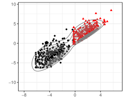
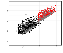
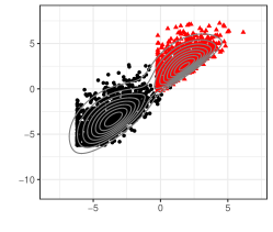
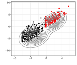
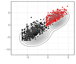
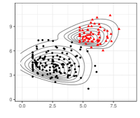
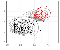
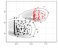
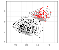
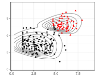
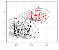
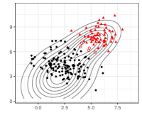
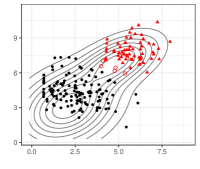
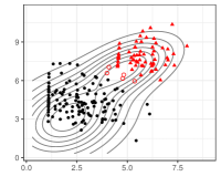
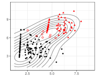
Figure 1 shows the simulated data from the FM-MSNC model with their respective density contours for the skew-normal (top panel) and normal (bottom panel) distributions and the allocations in each group for samples sizes , and with left-censoring proportion of . The black points represent the first component and the red triangles represent the second component of the mixture. One can note that the contour lines of the skew-normal distribution are more appropriate to represent the shape assumed by the generated data.
The results are presented in Table LABEL:tab:results_simu1. This table shows that, regardless the sample size, the Monte Carlo mean of the parameter estimates deviates further the true values as the censoring level increases, i.e., the parameter estimates are affected by the censoring level. In particular, the estimates of and appear to be less affected by increasing the censoring level than the other parameters. Furthermore, the estimates of the standard errors, i.e., MC Sd and IM SE, provide relatively close results, which may indicate that the asymptotic approach proposed for the standard errors of the ML estimates is reliable.
| Censoring | Measure | Parameter | ||||||||
|---|---|---|---|---|---|---|---|---|---|---|
| 1 | True | () | () | () | () | () | () | () | () | |
| MC mean | -3.1797 | -4.1235 | 1.6262 | 0.2923 | 2.2499 | -1.7236 | 2.1533 | 0.6607 | ||
| MC Sd | 0.3101 | 0.3705 | 0.1510 | 0.1138 | 0.1906 | 0.5262 | 0.5739 | 0.0274 | ||
| IM SE | 0.2844 | 0.3406 | 0.1361 | 0.0924 | 0.1944 | 0.5397 | 0.6202 | 0.0236 | ||
| 2 | True | () | () | () | () | () | () | () | ||
| MC mean | 2.0196 | 2.0954 | 1.3152 | 0.3177 | 1.7883 | -2.7361 | 3.7058 | |||
| MC Sd | 0.2381 | 0.2808 | 0.1431 | 0.0928 | 0.1595 | 1.0896 | 1.3303 | |||
| IM SE | 0.2677 | 0.2922 | 0.1391 | 0.0981 | 0.1816 | 1.2411 | 1.5434 | |||
| 1 | True | () | () | () | () | () | () | () | () | |
| MC mean | -3.3139 | -4.1708 | 1.5445 | 0.3483 | 2.2909 | -1.3744 | 2.0529 | 0.7030 | ||
| MC Sd | 0.3360 | 0.4545 | 0.1580 | 0.1413 | 0.2700 | 0.5082 | 0.7388 | 0.0238 | ||
| IM SE | 0.4719 | 0.5176 | 0.2080 | 0.1396 | 0.2762 | 0.7304 | 0.8737 | 0.0238 | ||
| 2 | True | () | () | () | () | () | () | () | ||
| MC mean | 2.2651 | 2.5165 | 1.3373 | 0.2533 | 1.6079 | -2.3831 | 3.1945 | |||
| MC Sd | 0.5131 | 0.5107 | 0.2661 | 0.1682 | 0.2207 | 1.5120 | 1.4642 | |||
| IM SE | 0.3213 | 0.3134 | 0.1929 | 0.1202 | 0.1726 | 1.4296 | 1.4575 | |||
| 1 | True | () | () | () | () | () | () | () | () | |
| MC mean | -3.1812 | -4.1450 | 1.6219 | 0.2804 | 2.2407 | -1.6988 | 2.1169 | 0.6594 | ||
| MC Sd | 0.1876 | 0.2248 | 0.0911 | 0.0615 | 0.1354 | 0.3611 | 0.4228 | 0.0165 | ||
| IM SE | 0.1988 | 0.2351 | 0.0962 | 0.0607 | 0.1369 | 0.3660 | 0.4177 | 0.0167 | ||
| 2 | True | () | () | () | () | () | () | () | ||
| MC mean | 2.0488 | 2.1190 | 1.3265 | 0.3071 | 1.7823 | -2.6601 | 3.5305 | |||
| MC Sd | 0.1698 | 0.2069 | 0.0912 | 0.0683 | 0.1091 | 0.6830 | 0.8175 | |||
| IM SE | 0.1938 | 0.2113 | 0.0994 | 0.0676 | 0.1266 | 0.7723 | 0.9274 | |||
| 1 | True | () | () | () | () | () | () | () | () | |
| MC mean | -3.3168 | -4.2133 | 1.5402 | 0.3276 | 2.2758 | -1.3758 | 2.0334 | 0.7021 | ||
| MC Sd | 0.2029 | 0.2736 | 0.0978 | 0.0776 | 0.1758 | 0.3513 | 0.5272 | 0.0162 | ||
| IM SE | 0.3071 | 0.3289 | 0.1374 | 0.0878 | 0.1840 | 0.4791 | 0.5681 | 0.0160 | ||
| 2 | True | () | () | () | () | () | () | () | ||
| MC mean | 2.3043 | 2.5243 | 1.3347 | 0.2208 | 1.5994 | -2.3618 | 3.0762 | |||
| MC Sd | 0.3216 | 0.2956 | 0.1899 | 0.1000 | 0.1513 | 1.0722 | 0.8913 | |||
| IM SE | 0.2144 | 0.2025 | 0.1295 | 0.0743 | 0.1172 | 0.8982 | 0.8670 | |||
| 1 | True | () | () | () | () | () | () | () | () | |
| MC mean | -3.2080 | -4.1723 | 1.6098 | 0.2779 | 2.2581 | -1.6429 | 2.1188 | 0.6600 | ||
| MC Sd | 0.1577 | 0.1728 | 0.0678 | 0.0525 | 0.1010 | 0.2864 | 0.3225 | 0.0118 | ||
| IM SE | 0.1411 | 0.1681 | 0.0672 | 0.0429 | 0.0978 | 0.2515 | 0.2926 | 0.0118 | ||
| 2 | True | () | () | () | () | () | () | () | ||
| MC mean | 2.0480 | 2.1143 | 1.3204 | 0.3059 | 1.7857 | -2.5958 | 3.4666 | |||
| MC Sd | 0.1283 | 0.1995 | 0.0642 | 0.0553 | 0.0845 | 0.5176 | 0.6986 | |||
| IM SE | 0.2882 | 0.3822 | 0.0739 | 0.0501 | 0.0888 | 0.6434 | 0.8032 | |||
| 1 | True | () | () | () | () | () | () | () | () | |
| MC mean | -3.3559 | -4.2548 | 1.4775 | 0.3046 | 2.1378 | -1.3237 | 2.0660 | 0.7036 | ||
| MC Sd | 0.1785 | 0.2527 | 0.1310 | 0.0859 | 0.3274 | 0.2934 | 0.4413 | 0.0109 | ||
| IM SE | 0.2138 | 0.2299 | 0.0921 | 0.0641 | 0.1320 | 0.3289 | 0.4023 | 0.0113 | ||
| 2 | True | () | () | () | () | () | () | () | ||
| MC mean | 2.2991 | 2.5248 | 1.3155 | 0.2141 | 1.6032 | -2.2326 | 2.9887 | |||
| MC Sd | 0.2436 | 0.2913 | 0.1381 | 0.0824 | 0.1245 | 0.7816 | 0.7760 | |||
| IM SE | 0.1601 | 0.1569 | 0.0922 | 0.0542 | 0.0847 | 0.5911 | 0.5862 | |||
5.2 Performance of the ML Estimates over missing data
In order to evaluate the performance of FM-MSNC model for dealing with partially incomplete data, a simulation study was conducted. Various ways of using models for imputation are described in Little and Rubin (2002), among them, one of the most relevant is the missing completely at random (MCAR). We simulated several datasets considering mixtures with two components from model (25) with two missing data proportion settings ( and ), taken in each mixture component, and different samples sizes . For each combination, we generated Monte Carlo (MC) samples. Summary statistics of the estimates across the MC samples were computed, such as the mean estimate (MC mean), the empirical standard error (MC Sd), and the mean of the approximate standard errors of the estimates, obtained through the method described in Section 4.3 (IM SE). We consider small and different variances with the following parameter as in the simulation about asymptotic properties in 5.5.
Table LABEL:tab:results_simu2 shows the results for this simulation. The results obtained are similar to those of simulation 5.1 and the same conclusions can be drawn. Additionally, we note that estimates appear to be more strongly affected as we increase the proportion of missing data in the sample.
| Missing | Measure | Parameter | ||||||||
|---|---|---|---|---|---|---|---|---|---|---|
| 1 | True | () | () | () | () | () | () | () | () | |
| MC mean | -5.2150 | -3.3411 | 1.6844 | 0.4594 | 1.9442 | -1.0396 | 1.4896 | 0.6495 | ||
| MC Sd | 0.5773 | 0.8843 | 0.1075 | 0.2005 | 0.2071 | 1.0020 | 1.5677 | 0.0219 | ||
| IM SE | 0.8618 | 0.9443 | 0.2666 | 0.1876 | 0.2603 | 0.9352 | 1.0664 | 0.0220 | ||
| 2 | True | () | () | () | () | () | () | () | ||
| MC mean | 1.7699 | 3.4694 | 1.3709 | 0.4857 | 1.7308 | -0.9892 | 1.5876 | |||
| MC Sd | 0.5614 | 0.7703 | 0.1231 | 0.1904 | 0.1922 | 1.1875 | 1.6737 | |||
| IM SE | 0.8408 | 0.9545 | 0.2759 | 0.2176 | 0.3247 | 1.2244 | 1.3864 | |||
| 1 | True | () | () | () | () | () | () | () | () | |
| MC mean | -5.2797 | -3.2378 | 1.6751 | 0.4903 | 1.9116 | -0.8182 | 1.1958 | 0.6495 | ||
| MC Sd | 0.6079 | 0.9007 | 0.1120 | 0.1908 | 0.2215 | 0.9494 | 1.5060 | 0.0228 | ||
| IM SE | 1.0618 | 1.1557 | 0.3267 | 0.2297 | 0.3216 | 1.1195 | 1.2620 | 0.0227 | ||
| 2 | True | () | () | () | () | () | () | () | ||
| MC mean | 1.6992 | 3.5252 | 1.3680 | 0.5125 | 1.7031 | -0.7323 | 1.3092 | |||
| MC Sd | 0.5987 | 0.7648 | 0.1359 | 0.1924 | 0.2047 | 1.1693 | 1.5322 | |||
| IM SE | 1.2860 | 1.4228 | 0.3530 | 0.2721 | 0.4106 | 1.6672 | 1.7740 | |||
| 1 | True | () | () | () | () | () | () | () | () | |
| MC mean | -5.1275 | -3.2608 | 1.6902 | 0.4589 | 1.9299 | -1.0984 | 1.4147 | 0.6493 | ||
| MC Sd | 0.5118 | 0.9054 | 0.0931 | 0.2000 | 0.1867 | 0.9515 | 1.5788 | 0.0188 | ||
| IM SE | 0.6699 | 0.7212 | 0.2189 | 0.1539 | 0.2158 | 0.7571 | 0.8440 | 0.0186 | ||
| 2 | True | () | () | () | () | () | () | () | ||
| MC mean | 1.8256 | 3.4568 | 1.3733 | 0.4711 | 1.7356 | -1.1133 | 1.6816 | |||
| MC Sd | 0.4959 | 0.7484 | 0.1053 | 0.1725 | 0.1741 | 1.0682 | 1.5869 | |||
| IM SE | 0.6973 | 0.8268 | 0.2228 | 0.1766 | 0.2621 | 1.0000 | 1.1773 | |||
| 1 | True | () | () | () | () | () | () | () | () | |
| MC mean | -5.1948 | -3.2079 | 1.6799 | 0.4817 | 1.8994 | -0.9175 | 1.1938 | 0.6488 | ||
| MC Sd | 0.5467 | 0.8905 | 0.0937 | 0.1907 | 0.1882 | 0.9160 | 1.4792 | 0.0192 | ||
| IM SE | 0.8447 | 0.8977 | 0.2686 | 0.1866 | 0.2680 | 0.9194 | 1.0006 | 0.0192 | ||
| 2 | True | () | () | () | () | () | () | () | ||
| MC mean | 1.7787 | 3.5349 | 1.3666 | 0.4987 | 1.7052 | -0.8822 | 1.3254 | |||
| MC Sd | 0.5295 | 0.7466 | 0.1172 | 0.1741 | 0.1832 | 1.0146 | 1.4570 | |||
| IM SE | 0.9450 | 1.0692 | 0.2765 | 0.2118 | 0.3275 | 1.2557 | 1.3766 | |||
| 1 | True | () | () | () | () | () | () | () | () | |
| MC mean | -5.1377 | -3.4011 | 1.6847 | 0.4243 | 1.9552 | -1.1829 | 1.6348 | 0.6488 | ||
| MC Sd | 0.4678 | 0.8574 | 0.0794 | 0.1869 | 0.1790 | 0.8858 | 1.4904 | 0.0169 | ||
| IM SE | 0.4769 | 0.4857 | 0.1699 | 0.1183 | 0.1781 | 0.5865 | 0.6471 | 0.0163 | ||
| 2 | True | () | () | () | () | () | () | () | ||
| MC mean | 1.8644 | 3.3518 | 1.3744 | 0.4342 | 1.7513 | -1.2648 | 1.9203 | |||
| MC Sd | 0.4578 | 0.6741 | 0.0891 | 0.1616 | 0.1540 | 0.9946 | 1.4206 | |||
| IM SE | 0.5043 | 0.5860 | 0.1656 | 0.1297 | 0.1999 | 0.7796 | 0.9222 | |||
| 1 | True | () | () | () | () | () | () | () | () | |
| MC mean | -5.2002 | -3.3434 | 1.6760 | 0.4495 | 1.9244 | -0.9997 | 1.4014 | 0.6485 | ||
| MC Sd | 0.5123 | 0.8387 | 0.0839 | 0.1816 | 0.1866 | 0.8815 | 1.4234 | 0.0175 | ||
| IM SE | 0.6459 | 0.6892 | 0.2138 | 0.1502 | 0.2198 | 0.7351 | 0.8213 | 0.0168 | ||
| 2 | True | () | () | () | () | () | () | () | ||
| MC mean | 1.7946 | 3.4393 | 1.3699 | 0.4709 | 1.7147 | -0.9902 | 1.5475 | |||
| MC Sd | 0.5079 | 0.6797 | 0.0986 | 0.1640 | 0.1650 | 1.0069 | 1.3840 | |||
| IM SE | 0.7262 | 0.7971 | 0.2178 | 0.1622 | 0.2598 | 1.0105 | 1.0992 | |||
To exemplify the predictive accuracies on the imputation of missing values, we compare the FM-MSNC with the traditional randomization-based mean imputation (MI) predictor Little and Rubin (2002), known as a common heuristic by filling in a single value for each missing value with the observed sample mean of the associated attribute. As a measure of precision, we use the mean absolute error (MAE) and the mean absolute relative error (MARE). They are defined as
| (32) |
where is the number of missing entries, is the actual value and is the respective predictive value. The MAE and MARE measures, for both FM-MSCN and MI method, are listed in Table 3. We can see that the FM-MSCN predictor exhibits considerable promising accuracy in the prediction of missing values when compared with those of MI imputations for all cases.
| Imputation method | Missing rate() | MAE | MARE | ||||
|---|---|---|---|---|---|---|---|
| 500 | 700 | 900 | 500 | 700 | 900 | ||
| FM-MSNC | 1.9009 | 1.8556 | 1.8444 | 0.8642 | 0.8747 | 0.8252 | |
| 2.0681 | 2.0243 | 2.0025 | 0.9883 | 1.0274 | 0.9678 | ||
| 2.4074 | 2.3693 | 2.3605 | 1.2264 | 1.2386 | 1.2345 | ||
| MI | 3.2550 | 3.0297 | 2.7708 | 1.6897 | 1.8542 | 1.5337 | |
| 3.2594 | 3.0498 | 2.7717 | 1.7402 | 1.8841 | 1.5501 | ||
| 3.2567 | 3.0563 | 2.7733 | 1.9881 | 1.8875 | 1.6624 | ||
5.3 Number of mixture components
In this section, we compare the ability of some classic model selection criteria discussed in Subsection 4.2 to select the appropriate model. One may argue that an arbitrary multivariate density can always be approximated by a finite mixture of normal multivariate distributions, see (Peel and McLachlan, 2000a, Chapter 1), for example. Thus, an interesting comparison can be made if we consider a sample from a two-component FM-MSNC(2) and use some model choice criteria to compare this model with the FM-MNC and several components under different censoring levels. Here we consider samples of size from a two-component FM-MSNC(2) model with left censoring levels at , or , and parameter values set at
The results are presented in Table 4, under different censoring levels, where it can be seen that all criteria favor the true model, that is, the FM-MSNC(2) model instead the FM-MNC model with two, three and four components, as expected. This is evidence that these measures are capable of detecting departures from normality. It is important to emphasize that the FM-MNC models with three and four components have and parameters respectively, while the FM-MSNC(2) model has parameters.
| Censoring | ||||||||||
|---|---|---|---|---|---|---|---|---|---|---|
| Group | 2 | 3 | 4 | 2 | 3 | 4 | 2 | 3 | 4 | |
| Criteria | AIC | 100 | 100 | 100 | 95 | 100 | 100 | 100 | 100 | 100 |
| BIC | 100 | 100 | 100 | 93 | 100 | 100 | 100 | 100 | 100 | |
| EDC | 100 | 100 | 100 | 93 | 100 | 100 | 100 | 100 | 100 | |
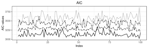
As pointed out for an anonymus referee, we can see in Table 4 that the case with censoring and two components is the only case where the correct model was not preferred by model selection criteria for a small number of instances. According to Figure 2, the preferred model in these (atypical) cases was the FM-MNC(2), however the differences in the criteria values related to a FM-MSNC(2) are close to zero. We believe that the amount of data sets generated in the simulation ( data sets) may not be sufficient and a more intensive simulation study would be required. However, due to the computational burden of the simulation, it would be too time consuming to move over to bigger simulations, say, data sets.


5.4 Clustering
Mixture models in general can be used for two main purposes: 1. estimation, and 2. model-based clustering McLachlan and Peel (2000). In this section, we investigate the ability of the FM-MSNC model to cluster observations, that is, to allocate them into groups of observations that are similar in some sense. We know that each data point belongs to heterogeneous populations, but we don’t know how to discriminate between them. Fitting the data with mixture models allows clustering the data in terms of the estimated posterior probability that a single point belongs to a given group. For this purpose, we follow the method proposed by Zeller et al. (2016), to assess the quality of the clustering of each mixture model using an index measure called correct classification rate (CCR), which is based on the posterior assigned to each subject. For the investigation of the clustering ability of the FM-MSNC model, we simulated MC samples considering mixtures with two components from model (24), with sample size , without censoring and left-censoring proportion settings taken in each mixture component, and parameter values set at
To fit the data we used the models FM-MSNC and FM-MNC amd for each model we obtain the estimate of the posterior probability that an observation belongs to the th component of the mixture, . So, if occurs in component , then is classified into group . For the th sample of the MC, we computed the correct classification rate, denoted by CCRm, then obtained the average of the correct classification rate (ACCR) of CCRm. Table 5 shows the ACCR values. From this table it is possible to observe that the model produces a high correct classification rate in both fitted models. We see that the rate decreases when the censoring proportion increases, this decrease is stronger for . Looking at the samples, keeping the censoring proportion fixed, the rate increased when the sample size increased.
| n | FM-MSNC | FM-MNC | |||||||
|---|---|---|---|---|---|---|---|---|---|
| 100 | 0.9685 | 0.9619 | 0.9558 | 0.945 | 0.8801 | 0.8809 | 0.8772 | 0.8735 | |
| 200 | 0.9729 | 0.9661 | 0.9599 | 0.9508 | 0.9206 | 0.9191 | 0.916 | 0.9016 | |
| 300 | 0.9733 | 0.9661 | 0.9608 | 0.9545 | 0.9248 | 0.9229 | 0.9233 | 0.9155 | |
Figure 3 shows the allocations in each group for sample size and left-censoring proportion of ,, and , where the groups are represented by black and red points. The first line of graphics (a - d) contains the scatter plot of the generated real data, where the black circles represent an observation erroneously classified as belonging to the black group. The second line of graphics (e - h) contains the scatter plot of the fitted FM-MSNC model, where the black circles represent an observation erroneously classified as belonging to the black group. The last line of graphics (i - l) contains the scatter plot of the fitted FM-MNC model, where the red circles represent an observation erroneously classified as belonging to the red group.
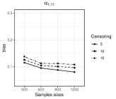
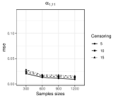
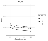
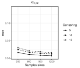
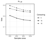
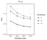
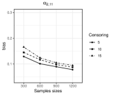
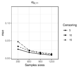
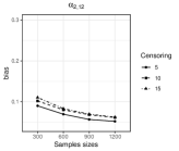
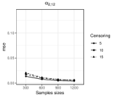
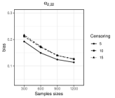
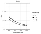
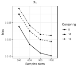
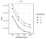
5.5 Asymptotic properties
In this simulation study, we analyze the absolute bias and the mean square error (mse) of the estimates obtained from the FM-MSNC model through the proposed EM algorithm. The idea of this simulation is to provide empirical evidence about the consistency of the ML estimates. These measures are defined by
| (33) |
where is the number of MC samples, and is the estimated ML of the parameter for the th sample. Four different sample sizes are considered. For each sample size, we generated Monte Carlo samples with censoring proportion. Using the EM algorithm, the absolute bias and mean squared error for each parameter over the datasets were computed. The parameter setup is as follows

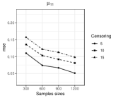
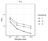
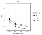
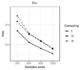
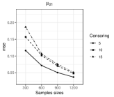
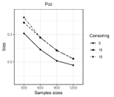
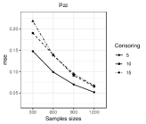
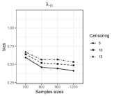
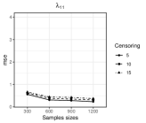
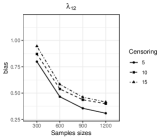
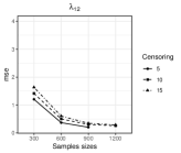
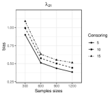
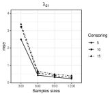

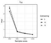
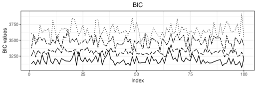
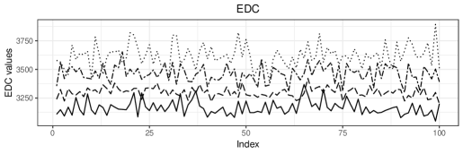
The results of the estimates of and are shown in Figures 4, 5, and 6. As a general rule, we can say that the and tend to approach zero when the sample size increases, indicating that the estimates based on the proposed EM algorithm, under the FM-MSNC model, provide good asymptotic properties.
6 Application
To illustrate the performance of our proposed model and algorithm, we consider a dataset of trace metal concentrations collected by the Virginia Department of Environmental Quality (VDEQ) that was previously analyzed by He (2013) and Lachos et al. (2017) using the normal and Student-t distribution, respectively.
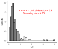
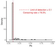
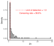
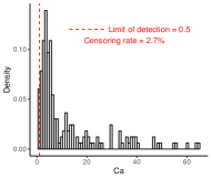
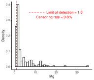
This dataset consists of concentration levels of dissolved trace metals in independently selected freshwater streams across the Commonwealth of Virginia. The five attributes are trace metals: copper (Cu), lead (Pb), zinc (Zn), calcium (Ca) and magnesium (Mg). The Cu, Pb, and Zn concentrations are reported in g/L of water, whereas Ca and Mg concentrations are reported in mg/L of water. Since the measurements were taken at different times, the presence of multiple limits of detection values are possible for each trace metal Richmond (2003). The limits of detection for Cu and Pb are both the g/L, g/L for Zn, while Ca and Mg have limits of mg/L and mg/L, respectively.
The percentage of left-censored values of for (Ca), for (Cu), for (Mg) are small in comparison to for (Pb) and for (Zn). Also note that of the streams had non-detected trace metals, had , had , had , had and had . As the concentration levels are strictly positive measures, to guarantee this, we consider an interval-censoring analysis by setting all lower limits of detection equal to for all trace metals. Also, due to the different scales for each trace metal, we standardize the dataset to have zero mean and variance equal to one as in Wang et al. (2019). The work mentioned before considered this dataset to be left censored without taking into account the possibility of predicting negative concentration levels for the trace metals. For instance, note that Pb censored concentrations take values in the small interval . Thus, after transforming the data, the new limits of detection are (Cu), (Pb), (Zn), (Ca), (Mg). Figure 7 shows the histogram for each original trace metal with the detection limits and all of them together.It can be seen that most of the distributions associated with the variables have two or more modes and are right skewed. For this reason we propose to fit a FM-MSNC model.

We fit the data with 1, 2 and 3 components considering the FM-MSNC, FM-MtC and FM-MNC models, for the FM-MtC model we consider fixed degrees of freedom, as described in Lachos et al. (2017). The number of groups of the model is chosen according to the information criteria as shown in Table 6. It can be seen that according to all model selection criteria the FM-MSNC model with three components fits the data best. We considered the variance-covariance to be equal in order to reduce the number of parameters to be estimated (parsimonious model).
| FM-MSNC | FM-MNC | ||||||
| Criteria | |||||||
| Log-likelihood | -1269.302 | -910.3387 | -697.6815 | -1351.596 | -1268.848 | -1210.626 | |
| AIC | 2588.604 | 1892.677 | 1489.363 | 2743.192 | 2589.695 | 2485.253 | |
| BIC | 2668.977 | 2008.415 | 1640.465 | 2807.491 | 2673.284 | 2588.13 | |
| EDC | 2606.427 | 1918.343 | 1522.871 | 2757.451 | 2608.232 | 2508.066 | |
| Time | 1.7023 min. | 4.0229 min. | 9.2552 min. | 1.054 sec. | 7.729 sec. | 26.0381 sec. | |
| FM-MtC | |||||||
| Criteria | |||||||
| Log-likelihood | -1040.276 | -1018.943 | -1074.852 | -1061.702 | -1036.393 | -1072.487 | |
| AIC | 2120.553 | 2089.887 | 2213.705 | 2163.404 | 2124.786 | 2208.974 | |
| BIC | 2184.852 | 2173.475 | 2316.583 | 2227.702 | 2208.375 | 2311.852 | |
| EDC | 2134.812 | 2108.423 | 2236.519 | 2177.662 | 2143.323 | 2231.788 | |
| Time | 16.672 sec. | 35.9952 sec. | 2.8734 min. | 13.1202 sec. | 29.9673 sec. | 2.68 min. | |
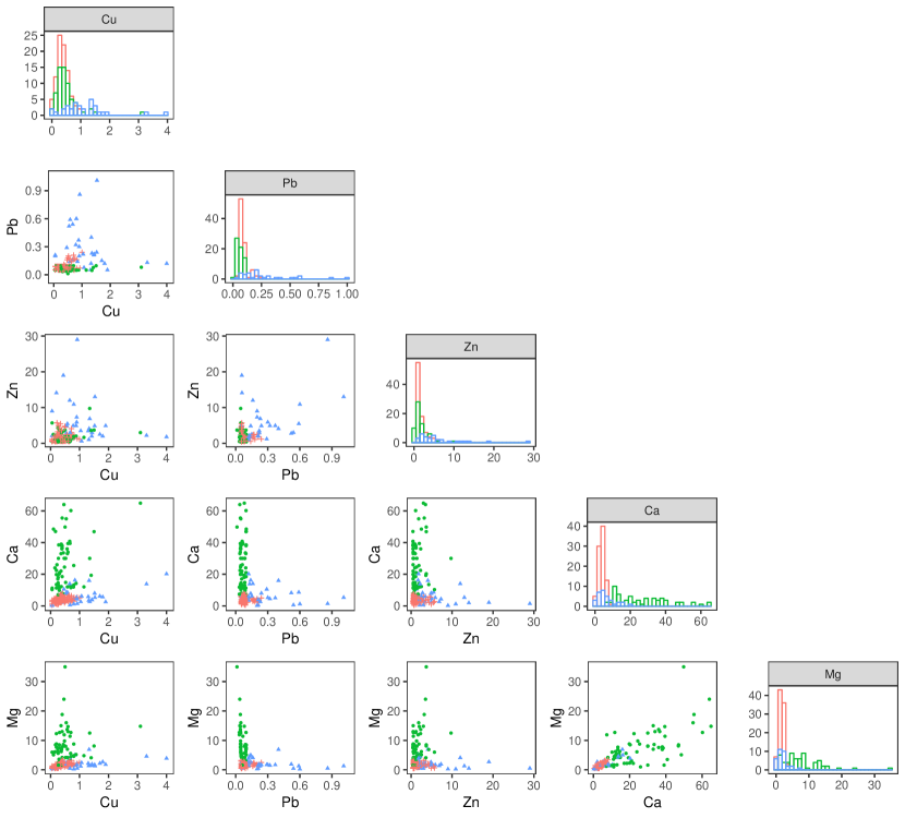
The ML estimates of the parameters were obtained using the EM algorithm described in Subsection 4.1. The results are shown in Table 7. As can be seen, of the freshwater streams belong to Cluster 1, Cluster 2 contains around of them and the remaining belong to Cluster 3. Table 6 shows that the best FM-MNC model has two components, and in this of freshwater streams belong to Cluster 1 and the remaining are in Cluster 2. For the FM-MtC model, the best model also has two components and three degrees of freedom. In this case, of freshwater streams belong to Cluster 1 and the remaining belong to Cluster 2.
| Parameter | Estimate |
|---|---|
In Figure 8, we fit the data using the FM-MSNC with three components. The scatter plots of the observations for each pair of trace metals reveal that it is difficult to classify freshwater streams by visualization because these observations almost mix together.
7 Conclusions
In this paper, a novel approach to analyze multiply censored and missing data is presented based on the use of finite mixtures of multivariate skew-normal distributions. This approach generalizes
several previously proposed solutions for censored data, such as, the finite mixture of Gaussian components (Karlsson and Laitila, 2014; Caudill, 2012; He, 2013) and the finite mixture of Student-t components (Lachos et al., 2017), which are also restricted to a left or right censored problem. A simple and efficient EM-type algorithm was developed, which has closed-form expressions at the
E-step and relies on formulas for the mean vector and covariance matrix of the
multivariate truncated skew-normal distribution, for which the the R MomTrunc library is used (Galarza et al., 2020). The proposed EM algorithm was implemented as part of the R package CensMFM and is
available for download at the CRAN repository. The experimental results and
the analysis of a real dataset provide support for the usefulness and effectiveness of our proposal.
The method proposed in this paper can be extended to other types of mixture distributions, for example, the multivariate scale mixtures of skew-normal distributions (Cabral et al., 2012) or generalized hyperbolic mixtures (Browne and McNicholas, 2015). It is also of interest to develop an effective Markov chain Monte Carlo algorithm for the FM-MSNC models in a fully Bayesian treatment. Finally, the proposed methods can also be easily applied to other substantial areas in which the data being analyzed have censored and/or missing observations, for instance, factor analysis models (Wang et al., 2017) and linear mixed models (Lin et al., 2009; Lachos et al., 2011).
References
- Akaike [1974] Akaike H (1974) A new look at the statistical model identification. IEEE Trans Autom Cont 19:716–723
- Arellano-Valle and Genton [2005] Arellano-Valle RB, Genton MG (2005) On fundamental skew distributions. Journal of Multivariate Analysis 96:93–116
- Arellano-Valle and Genton [2010] Arellano-Valle RB, Genton MG (2010) Multivariate extended skew-t distributions and related families. Metron LXVIII:201–234
- Azzalini and Capitanio [1999] Azzalini A, Capitanio A (1999) Statistical applications of the multivariate skew-normal distribution. Journal of the Royal Statistical Society, Series B 61:579–602
- Azzalini and Dalla-Valle [1996] Azzalini A, Dalla-Valle A (1996) The multivariate skew-normal distribution. Biometrika 83(4):715–726
- Bai et al. [1989] Bai Z, Krishnaiah P, Zhao L (1989) On rates of convergence of efficient detection criteria in signal processing with white noise. Inform Theory IEEE Trans 35:380–388
- Basford et al. [1997] Basford K, Greenway D, McLachlan G, Peel D (1997) Standard errors of fitted component means of normal mixtures. Computational Statistics 12:1–18
- Basso et al. [2010] Basso RM, Lachos VH, Cabral CRB, Ghosh P (2010) Robust mixture modeling based on scale mixtures of skew-normal distributions. Computational Statistics & Data Analysis 54(12):2926–2941
- Bouveyron et al. [2019] Bouveyron C, Celeux G, Murphy T, Raftery A (2019) Model-Based Clustering and Classification for Data Science: With Applications in R. Cambridge University Press
- Browne and McNicholas [2015] Browne RP, McNicholas PD (2015) A mixture of generalized hyperbolic distributions. Canadian Journal of Statistics 43(2):176–198
- Cabral et al. [2012] Cabral CRB, Lachos VH, Prates MO (2012) Multivariate mixture modeling using skew-normal independent distributions. Computational Statistics & Data Analysis 56:126–142
- Caudill [2012] Caudill SB (2012) A partially adaptive estimator for the censored regression model based on a mixture of normal distributions. Statistical Methods & Applications 21:121–137
- Dempster et al. [1977] Dempster A, Laird N, Rubin D (1977) Maximum likelihood from incomplete data via the EM algorithm. Journal of the Royal Statistical Society, Series B 39:1–38
- Frühwirth-Schnatter [2006] Frühwirth-Schnatter S (2006) Finite mixture and Markov switching models. Springer Science & Business Media
- Galarza et al. [2020] Galarza CE, Kan R, Lachos VH (2020) MomTrunc: Moments of Folded and Doubly Truncated Multivariate Distributions. R Package Version 5.87 URL http://CRANR-projectorg/package=MomTrunc
- He [2013] He J (2013) Mixture model based multivariate statistical analysis of multiply censored environmental data. Advances in Water Resources 59:15–24
- Karlsson and Laitila [2014] Karlsson M, Laitila T (2014) Finite mixture modeling of censored regression models. Statistical Papers 55(3):627–642
- Lachos et al. [2011] Lachos VH, Bandyopadhyay D, Dey DK (2011) Linear and nonlinear mixed-effects models for censored HIV viral loads using normal/independent distributions. Biometrics 67:1594–1604
- Lachos et al. [2017] Lachos VH, Moreno EJL, Chen K, Cabral CRB (2017) Finite mixture modeling of censored data using the multivariate Student-t distribution. Journal of Multivariate Analysis 159:151–167
- Lachos et al. [2018] Lachos VH, Cabral CRB, Zeller CB (2018) Finite Mixture of Skewed Distributions. Springer
- Lin [2009] Lin TI (2009) Maximum likelihood estimation for multivariate skew normal mixture models. Journal of Multivariate Analysis 100(2):257–265
- Lin et al. [2009] Lin TI, Ho HJ, Chen CL (2009) Analysis of multivariate skew normal models with incomplete data. Journal of Multivariate Analysis 100(19):2337–2351
- Lin and Wang [2019] Lin TI, Wang WL (2019) Multivariate-t linear mixed models with censored responses, intermittent missing values and heavy tails. Statistical Methods in Medical Research p 0962280219857103
- Lin et al. [2018] Lin TI, Lachos VH, Wang WL (2018) Multivariate longitudinal data analysis with censored and intermittent missing responses. Statistics in Medicine 37(19):2822–2835
- Little and Rubin [2002] Little RJ, Rubin DB (2002) Statistical analysis with missing data, vol 793. John Wiley & Sons
- Louis [1982] Louis TA (1982) Finding the observed information matrix when using the em algorithm. Journal of the Royal Statistical Society, Series B 44:226–233
- McLachlan and Krishnan [2008] McLachlan GJ, Krishnan T (2008) The EM Algorithm and Extensions, 2nd edn. Wiley
- McLachlan and Peel [2000] McLachlan GJ, Peel D (2000) Finite Mixture Models. Wiley, New York
- McNicholas [2016] McNicholas PD (2016) Mixture model-based classification. Chapman and Hall/CRC
- Meilijson [1989] Meilijson I (1989) A fast improvement to the em algorithm on its own terms. Journal of the Royal Statistical Society, Series B (Methodological) 51(1):127–138
- Peel and McLachlan [2000a] Peel D, McLachlan GJ (2000a) Finite Mixture Models. John Wiley & Sons
- Peel and McLachlan [2000b] Peel D, McLachlan GJ (2000b) Robust mixture modelling using the t distribution. Statistics and Computing 10(4):339–348
- Prates et al. [2013] Prates MO, Lachos VH, Cabral C (2013) mixsmsn: Fitting finite mixture of scale mixture of skew-normal distributions. Journal of Statistical Software 54(12):1–20
- Richmond [2003] Richmond V (2003) The quality of virginia non-tidal streams: First year report
- Schwarz [1978] Schwarz G (1978) Estimating the dimension of a model. The Annals of Statistics 6:461–464
- Wang et al. [2017] Wang WL, Liu M, Lin TI (2017) Robust skew-t factor analysis models for handling missing data. Statistical Methods & Applications 26(4):649–672
- Wang et al. [2019] Wang WL, Castro LM, Lachos VH, Lin TI (2019) Model-based clustering of censored data via mixtures of factor analyzers. Computational Statistics & Data Analysis 140:104–121
- Zeller et al. [2016] Zeller CB, Cabral CR, Lachos VH (2016) Robust mixture regression modeling based on scale mixtures of skew-normal distributions. Test 25(2):375–396