A unified meshfree pseudospectral method for solving both classical and fractional PDEs

Abstract

In this paper, we propose a meshfree method based on the Gaussian radial basis function (RBF) to solve both classical and fractional PDEs. The proposed method takes advantage of the analytical Laplacian of Gaussian functions so as to accommodate the discretization of the classical and fractional Laplacian in a single framework and avoid the large computational cost for numerical evaluation of the fractional derivatives. These important merits distinguish it from other numerical methods for fractional PDEs. Moreover, our method is simple and easy to handle complex geometry and local refinement, and its computer program implementation remains the same for any dimension $d\geq 1$. Extensive numerical experiments are provided to study the performance of our method in both approximating the Dirichlet Laplace operators and solving PDE problems. Compared to the recently proposed Wendland RBF method, our method exactly incorporates the Dirichlet boundary conditions into the scheme and is free of the Gibbs phenomenon as observed in the literature. Our studies suggest that to obtain good accuracy the shape parameter cannot be too small or too big, and the optimal shape parameter might depend on the RBF center points and the solution properties.

Keywords. Meshfree method, radial basis functions, fractional Laplacian, classical Laplacian, pseudospectral method, hypergeometric functions.

1 Introduction

In the recent decade, fractional partial differential equations (PDEs) have found widespread applications in many fields, including turbulence [8, 18, 17], geophysics [4, 47], biomedicine and biology [35, 27], and quantum mechanics [33, 11]. In traditional (integer-order) PDEs, diffusion describes the transport process due to Brownian motion and is modeled by the classical Laplacian $\Delta$. In contrast, diffusion in fractional PDEs is described by the fractional Laplacian $(-\Delta)^{\frac{\alpha}{2}}$ which underlines the Lévy transport. It was recently found that the Brownian and Lévy transports might coexist in many complex (e.g., biological and chemical) systems [4, 47, 27]. Thus mathematical models including both classical and fractional Laplacians could be more proper to describe such a phenomenon. On the other hand, the classical and fractional Laplacians, one local and the other nonlocal, possess distinct properties. Consequently, the analytical and numerical frameworks for studying these two operators are significantly different. For instance, numerical discretizations (e.g., finite element methods) for the classical and fractional Laplacians are usually incompatible, and separate implementation efforts are required to study problems of these two operators. In this work, we propose a new meshfree pseudospectral method with the intrinsic merit of solving both classical and fractional PDEs in a unified scheme.

The classical and fractional Laplacians can be defined via the parametric pseudo-differential operator with symbol $|\xi|^{\alpha}$ [32, 41]:

$$(-\Delta)^{\frac{\alpha}{2}}u({{\bf x}})=\mathcal{F}^{-1}\big{[}|\xi|^{\alpha}\mathcal{F}[u]\big{]},\qquad\mbox{for}\ \ \alpha\geq 0,$$ (1.1)

where $\mathcal{F}$ is the Fourier transform with associated inverse transform $\mathcal{F}^{-1}$. The definition (1.1) covers a wide class of operators for different values of the parameter $\alpha$. In this work, we are interested in the exponent $\alpha\in(0,2]$. For $\alpha=2$, the formulation (1.1) gives the spectral representation of the classical Laplacian $-\Delta$, while it is referred to as the fractional Laplacian if $\alpha<2$. Probabilistically, the fractional Laplacian represents the infinitesimal generator of a symmetric $\alpha$-stable Lévy process. It can be also defined in a hypersingular integral form (also known as the integral fractional Laplacian) [32, 41, 31]:

$$(-\Delta)^{\frac{\alpha}{2}}u({\bf x})=C_{d,\alpha}\,{\rm P.V.}\int_{{\mathbb{R}}^{d}}\frac{u({\bf x})-u({\bf y})}{|{\bf x}-{\bf y}|^{d+\alpha}}d{\bf y},\qquad\mbox{for}\ \ \alpha\in(0,2),$$ (1.2)

for $d=1,2$, or $3$, where ${\rm P.V.}$ stands for the principal value integral, and $|{\bf x}-{\bf y}|$ denotes the Euclidean distance between points ${\bf x}$ and ${\bf y}$. The normalization constant is given by

$$C_{d,\alpha}=\frac{2^{\alpha-1}\alpha\,\Gamma(({\alpha+d})/{2})}{\sqrt{\pi^{d}}\,\Gamma(1-{\alpha}/{2})}$$

with $\Gamma(\cdot)$ being the Gamma function. Over the entire space ${\mathbb{R}}^{d}$, the integral fractional Laplacian (1.2) is equivalent to the pseudo-differential operator (1.1) with $\alpha\in(0,2)$ [31, 41, 32].

The formulation in (1.1) provides a uniform definition of the classical and fractional Laplacians via the parametric symbol $|\xi|^{\alpha}$. It suggests that if the entire space ${\mathbb{R}}^{d}$ or periodic bounded domains are considered, one can study these two operators together. For example, the Fourier pseudospectral methods based on (1.1) were introduced in [12, 29] to solve the classical and fractional Schrödinger equations on a periodic domain. However, if a non-periodic bounded domain is considered, the pseudo-differential form of the classical and fractional Laplacians loses its advantages and has challenges to incorporate general boundary conditions. Thus different representations of the classical Laplacian (i.e. $\Delta=\partial_{xx}+\partial_{yy}+\partial_{zz}$) and fractional Laplacian (i.e. formulation in (1.2)) are adopted, which clearly manifests the differences between these two operators – one is a local derivative operator, and the other is a nonlocal integral operator. In practice, numerical methods (e.g., finite difference/element methods) for these two operators on domains with non-periodic boundary conditions are separately developed and incompatible.

Compared to the classical Laplacian, numerical methods for the fractional Laplacian (1.2) still remain limited. In [10, 13, 14], second-order finite difference methods were proposed to discretize the integral fractional Laplacian (1.2) for $d\geq 1$, and fast algorithms via the fast Fourier transforms were introduced for their efficient simulations. Various finite element methods based on different formulations of the fractional Laplacian were developed in [2, 1, 6, 3, 9] to solve fractional problems. Recently, spectral methods were proposed to solve fractional PDEs with the integral fractional Laplacian in bounded and unbounded domains [48, 44]. These spectral methods could achieve higher accuracy than finite difference/element methods, but they have limited usability on irregular domains. So far the existing numerical methods for the classical Laplacian and their computer implementations cannot be used to solve problems with the fractional Laplacian, due to the distinct features of these two operators.

On the other hand, meshfree methods based on radial basis functions (RBF) have been widely applied to solve classical PDEs [24, 19]. Compared to the mesh-based methods, these methods have more flexibility of domain geometry and can achieve higher accuracy with less computational cost. The application of RBF-based methods to solve fractional PDEs and nonlocal problems is still very recent. In [5, 34, 49], the Galerkin methods using a localized basis of RBFs were proposed to solve nonlocal diffusion problems. In [38], RBF-QR methods were proposed to solve the Riemann–Liouville spatial fractional diffusion problems. A Kansa RBF method was proposed in [37] to solve the fractional advection-dispersion equations, where the spatial derivative was defined via the fractional directional derivatives. Later, RBF collocation methods were introduced in [46] to solve similar advection-dispersion equations but with the Riesz spatial fractional derivatives. We remark that these RBF methods are for different fractional derivatives, and in this work we are interested in the fractional Laplacian. Recently, a Wendland RBF collocation method was proposed in [40] to solve fractional problems with the fractional Laplacian (1.1), while a singular boundary method based on a new definition of the fractional Laplacian was introduced in [7]. Note that all the above RBF methods developed in the fractional cases cannot be used to solve classical problems.

In this work, we propose a novel meshfree pseudospectral method based on the Gaussian RBFs, which has fundamental differences from other RBF-based methods in [5, 34, 49, 38, 37, 46, 40]. Inheriting the advantages of RBF methods, our method is simple and flexible of domain geometry, and its computer implementation remains the same for any dimension $d\geq 1$. Furthermore, it allows easy local refinements. Besides these advantages, our method has the distinct merits as below.

• It solves the classical and fractional PDEs in a unified scheme. To the best of our knowledge, this is the first numerical method that discretizes the classical and fractional Laplacians on non-periodic domains with a single scheme. This feature distinguishes our method from other existing methods which solve classical and fractional problems separately.

• It takes great advantage of the Laplacian of the Gaussian RBFs (i.e. the confluent hypergeometric function) and avoids large computational costs in approximating the fractional derivative of RBFs, which is one major difference from those in [38, 37, 46, 40]. The fractional derivatives are usually defined in integral form with a singular kernel. As pointed out in [37], it is challenging to balance the accuracy and efficiency in approximating the fractional derivatives of RBFs with quadrature rules (e.g., Gauss–Jacobi quadrature rules are used in [37]).

• It exactly incorporates the boundary conditions into the scheme and is free of the Runge phenomenon observed in [40]. In contrast to the method in [40], our method uses the exact boundary conditions and avoids evaluating the fractional Laplacian of RBFs with numerical quadrature rules. Moreover, the method in [40] requires a larger computational domain (much bigger than the actual physical domain), which significantly increases the computational costs especially for $d>1$.

The paper is organized as follows. In Section 2, we first outline some important properties of the Gaussian RBFs and then introduce our numerical method on a bounded domain with Dirichlet boundary conditions. The performance of our method in approximating the Laplace operators is studied in Section 3. We then apply it solve the classical and fractional PDE problems in Section 4. Finally, some discussion and summary are made in Section 5.

2 RBF meshfree method

Radial basis functions (RBFs) are well-known for their advantages in high-dimensional scattered data approximations and have recently broadened their applications in many areas, ranging from meteorology, statistics, to machine learning. RBFs are usually real-valued scalar functions defined in the form of $\varphi(|{\bf x}|)$, where $|{\bf x}|$ denotes the Euclidean norm of vector ${\bf x}\in{\mathbb{R}}^{d}$. This radial form (e.g., $r=|{\bf x}|$) makes their use for high-dimensional reconstruction problems very efficient and also allows invariance under orthogonal transforms. Common choices of RBFs usually fall into two main categories: globally-supported functions (e.g., Gaussian RBFs), and compactly-supported functions (e.g., Wendland RBFs). For more discussion of RBFs, we refer the reader to [24, 19] and references therein. In this work, we will use the Gaussian RBFs and start with some of their properties in Section 2.1.

2.1 Gaussian radial basis functions

Among all radial basis functions, the Gaussian RBF is a representative member of the class of infinitely differentiable functions with global support. It is defined as

$$\varphi(|{\bf x}|)=\exp(-\varepsilon^{2}|{\bf x}|^{2}),\qquad\mbox{for}\ \ {\bf x}\in{\mathbb{R}}^{d},$$

where $\varepsilon\in{\mathbb{R}}$ denotes the shape parameter. The shape parameter $\varepsilon$ plays an important role in the approximation accuracy with Gaussian RBFs. It is usually chosen to be a constant, and recently spatial-dependent shape parameters were studied in the literature [26].

When using RBF-based methods to solve fractional PDEs, the main challenge is to compute the fractional derivatives of RBFs [37, 40, 38]. Their analytical solutions are usually unavailable, so numerical approximations are required to evaluate these fractional derivatives, e.g., the Gauss–Jacobi quadrature rules were used in [37]. Note that the fractional derivatives are generally defined as an integral with singular kernel over a large domain. Therefore, using quadrature rules to approximate the fractional derivatives of RBFs significantly increases the computational costs, especially in high-dimensional problems. Moreover, it makes the implementation of RBF-based methods more complicated as special treatments are required around the singularity. These complications greatly deteriorate the performance of RBF-based methods in practice. In contrast, our method takes advantage of the properties of the Laplace operators and Gaussian RBFs so as to avoid numerical evaluations of the fractional derivatives with quadrature rules, which is one fundamental difference between our method and those in the literature [37, 40, 38].

To introduce our method, we will first present some important properties of the Laplace operators and their actions on Gaussian functions in the following lemmas.

Lemma 2.1 (The Laplacian of Gaussian functions).

Let $u$ be a Gaussian function of the form $u({\bf x})=\exp(-|{\bf x}|^{2})$, for ${\bf x}\in{\mathbb{R}}^{d}$. Then the Laplacian of $u$ is analytically given by [39, 16]:

$$(-\Delta)^{\frac{\alpha}{2}}u({\bf x})=\frac{2^{\alpha}\Gamma((d+\alpha)/2)}{\Gamma(d/2)}\,_{1}F_{1}\Big{(}\frac{d+\alpha}{2};\,\frac{d}{2};\,-|{\bf x}|^{2}\Big{)},\qquad\mbox{for}\ \ {\bf x}\in{\mathbb{R}}^{d},\quad\alpha\geq 0,$$ (2.1)

where ${}_{1}F_{1}$ denotes the confluent hypergeometric function.

Lemma 2.1 holds for any exponent $\alpha\geq 0$. It provides the foundation of developing unified schemes for the classical and fractional Laplacians. In the special case of $\alpha=2m$ with $m\in{\mathbb{N}}$, the result in (2.1) collapses to the classical integer-order derivatives $(-\Delta)^{m}e^{-|{\bf x}|^{2}}$. For instance, using the properties of the confluent hypergeometric function ${}_{1}F_{1}$, we obtain that (2.1) is equivalent to

$$-\Delta e^{-|{\bf x}|^{2}}=e^{-|{\bf x}|^{2}}(4|{\bf x}|^{2}-2d),\qquad\mbox{for}\ {\bf x}\in{\mathbb{R}}^{d},$$

when $\alpha=2$, i.e., the classical negative Laplacian of the Gaussian function.

Fig. 1 illustrates the result $(-\Delta)^{\frac{\alpha}{2}}u$ for various $\alpha\geq 0$, where $u(x)=e^{-x^{2}}$ for $x\in{\mathbb{R}}$. It shows that the function $(-\Delta)^{\frac{\alpha}{2}}u$ is “radially” symmetric with respect to $x=0$, confirming that the Laplace operator is rotationally invariant. The rotational invariance is a crucial property in modeling isotropic anomalous diffusion in many applications [13].

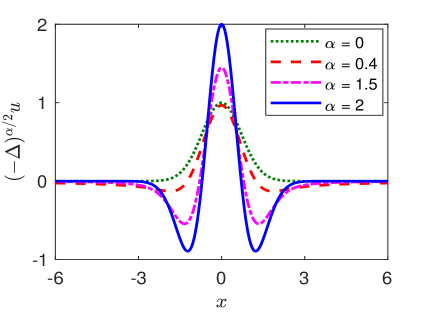
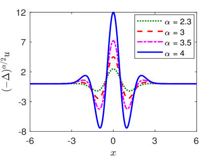
Figure 1: Illustration of function $(-\Delta)^{\frac{\alpha}{2}}u$ with $u(x)=\exp(-x^{2})$ for various $\alpha\geq 0$.

Moreover, the solution decays to zero as $|{\bf x}|\to\infty$ – the larger the exponent $\alpha$, the faster the decay. In the extreme case of $\alpha=0$, there is $(-\Delta)^{\frac{\alpha}{2}}u({\bf x})=u({\bf x})$, that is, $(-\Delta)^{\frac{\alpha}{2}}$ reduces to the identify operator $I$, consistent with the definition (1.1) as $\alpha\to 0$. Fig. 1 additionally shows that the function $(-\Delta)^{\frac{\alpha}{2}}$ has larger oscillations as $\alpha$ increases.

Besides Lemma 2.1, another important building block of our method is the properties of the Laplace operators as described below.

Lemma 2.2 (Properties of the Laplace operators).

For function $u$, assume the Laplacian function ${\mathcal{U}}({\bf x}):=(-\Delta)^{\frac{\alpha}{2}}u({\bf x})$ exists for ${\bf x}\in{\mathbb{R}}^{d}$. Then it satisfies the following properties [41]:

$$\displaystyle(-\Delta)^{\frac{\alpha}{2}}\big{[}u({\bf x}-{\bf x}_{0})\big{]}={\mathcal{U}}({\bf x}-{\bf x}_{0}),\qquad\mbox{for}\ \ \alpha\geq 0,$$ (2.2)

for any point ${\bf x}_{0}\in{\mathbb{R}}^{d}$, and

$$\displaystyle(-\Delta)^{\frac{\alpha}{2}}\big{[}u(\kappa{\bf x})\big{]}=|\kappa|^{\alpha}{\mathcal{U}}(\kappa{\bf x}),\qquad\mbox{for}\ \ \alpha\geq 0,$$ (2.3)

for constant $\kappa\in{\mathbb{R}}$.

Lemma 2.2 plays an important role in the design of our meshfree method, which allows us to find the analytical solution to the Laplacian of Gaussian RBFs with different shape parameters and center points. Combining (2.1)–(2.3), we immediately obtain that for any point ${\bf x}_{0}\in{\mathbb{R}}^{d}$ and shape parameter $\varepsilon\in{\mathbb{R}}$, there is

$$(-\Delta)^{\frac{\alpha}{2}}e^{-\varepsilon^{2}|{\bf x}-{\bf x}_{0}|^{2}}=c_{d,\alpha}|\varepsilon|^{\alpha}\,_{1}F_{1}\Big{(}\frac{d+\alpha}{2};\frac{d}{2};-\varepsilon^{2}|{\bf x}-{\bf x}_{0}|^{2}\Big{)},\qquad\mbox{for}\ \ \alpha\geq 0.$$ (2.4)

Here and in the following, we denote the constant $c_{d,\alpha}=2^{\alpha}\Gamma((d+\alpha)/2)/\Gamma(d/2)$, to be distinguished from $C_{d,\alpha}$ in (1.2). It shows that over the entire space ${\mathbb{R}}^{d}$, the classical and fractional Laplacian of Gaussian RBFs can be given in a unified form with parameter $\alpha$. As we will see in Section 2.2, this uniform structure in (2.4) provides the foundation to design the unified numerical methods for classical and fractional PDEs.

2.2 RBF discretization schemes

In the following, we will present our meshfree method to approximate the Laplace operator $(-\Delta)^{\frac{\alpha}{2}}$ and the related Poisson problems. Its generalization to time-dependent problems is straightforward (see Section 4.3). As mentioned previously, we will focus on the cases with $\alpha\in(0,2]$. Our method can be directly applied to discretize the operator $(-\Delta)^{2m}$ with $m\in{\mathbb{N}}$. Its generalization to the cases of $\alpha>2$ but $\alpha\neq 2m$ requires the point-wise definition of $(-\Delta)^{\frac{\alpha}{2}}$, such as (1.2) for $\alpha\in(0,2)$, which is beyond the scope of this work.

Let $\Omega\subset{\mathbb{R}}^{d}$ be an open bounded domain. We consider the following Poisson problem with Dirichlet boundary conditions:

$$(-\Delta)^{\frac{\alpha}{2}}u({\bf x})=f({\bf x}), \mbox{for \ ${\bf x}\in\Omega$},$$ (2.5)

$$u({\bf x})=g({\bf x}), \mbox{for \ ${\bf x}\in\Upsilon$}.$$ (2.6)

where we denote $\Upsilon=\partial{\Omega}$ for $\alpha=2$,  or $\Upsilon=\Omega^{c}={\mathbb{R}}^{d}\backslash\Omega$ if $\alpha<2$. If $\alpha=2$, the problem (2.5)–(2.6) becomes the classical Dirichlet Poisson problem. While $\alpha\in(0,2)$, it collapses to the fractional Poisson equation with extended Dirichlet boundary conditions on $\Omega^{c}$. So far most studies on the fractional Poisson problem focus on the homogeneous Dirichlet boundary conditions (i.e., $g({\bf x})\equiv 0$ in (2.6)); see [10, 13, 2, 6] and references therein. Here, we consider more general boundary conditions $g({\bf x})$. Usually, if non-periodic boundary conditions are considered, the classical and fractional Poisson problems are discretized and solved separately. To the best of our knowledge, this is the first work to solve the classical and fractional Poisson problems in a single $\alpha$-parametric scheme.

Let $N$ and $\bar{N}$ be two positive integers, and $N<\bar{N}$. Denote ${\bf x}_{i}$ (for $1\leq i\leq\bar{N}$) as pre-defined collocation points on $\bar{\Omega}=\Omega\cup\partial\Omega$. For simplicity, we introduce

$${\mathcal{S}}_{\Omega}=\{{\bf x}_{i}\in\Omega\mid 1\leq i\leq N\},\qquad{\mathcal{S}}_{\partial\Omega}=\{{\bf x}_{i}\in\partial{\Omega}\mid N+1\leq i\leq\bar{N}\}$$

to represent the set of points in domain $\Omega$ and on boundary $\partial\Omega$, respectively, and let ${\mathcal{S}}_{\bar{\Omega}}={\mathcal{S}}_{\Omega}\cup{\mathcal{S}}_{\partial\Omega}$. Assume that the function $u$ can be approximated by

$$u({\bf x})\approx\widehat{u}({\bf x}):=\sum_{i=1}^{\bar{N}}\lambda_{i}\,\varphi^{\varepsilon}(|{\bf x}-{\bf x}_{i}|),\qquad\mbox{for}\ \ {\bf x}\in\bar{\Omega},$$ (2.7)

where $\varphi^{\varepsilon}(|{\bf x}-{\bf x}_{i}|)$ represents the Gaussian RBF with shape parameter $\varepsilon$ and center point ${\bf x}_{i}$. For point ${\bf x}\notin\bar{\Omega}$, we assume that $u$ satisfies (2.6). Then the coefficients $\lambda_{i}$ can be found by applying (2.7) at a set of test points ${\bf x}_{k}\in{\mathcal{S}}_{\bar{\Omega}}$ that may or may not coincide with the center points. In the following, we will include a superscript to distinguish the center-point sets (i.e. ${\mathcal{S}}_{\Omega}^{c}$ and ${\mathcal{S}}_{\partial\Omega}^{c}$) and test-point sets (i.e. ${\mathcal{S}}_{\Omega}^{t}$ and ${\mathcal{S}}_{\partial\Omega}^{t}$). Note that the number of test points should be the same as that of center points, i.e., $|\mathcal{S}_{\bar{\Omega}}^{t}|=|{\mathcal{S}}_{\bar{\Omega}}^{c}|=\bar{N}$, to ensure a square linear system for $\lambda_{i}$.

First, we will derive the approximation of the Dirichlet Laplacian, i.e., a finite dimensional representation of the operator $(-\Delta)^{\frac{\alpha}{2}}$ with Dirichlet boundary conditions in (2.6). To facilitate our explanation, we will start with separate discussion for $\alpha=2$ and $\alpha<2$, demonstrating the difference between the classical and fractional Laplacians. Later, we will combine our results of $\alpha=2$ and $\alpha<2$ into a single $\alpha$-parametric scheme. The situation of the classical Laplacian is relatively simple, and combining (2.4) with (2.7) immediately leads to the approximation:

$$-\Delta_{h}u({\bf x})=-\Delta\widehat{u}({\bf x})=c_{d,2}|\varepsilon|^{2}\sum_{i=1}^{\bar{N}}\lambda_{i}\,{}_{1}F_{1}\Big{(}\frac{d}{2}+1;\frac{d}{2};-\varepsilon^{2}|{\bf x}-{\bf x}_{i}|^{2}\Big{)},\qquad\mbox{for}\ \ {\bf x}\in\Omega,$$ (2.8)

where $-\Delta_{h}$ denotes the numerical approximation of the operator $-\Delta$.

In contrast, the approximation to the fractional Laplacian (i.e. $\alpha<2$) is more complicated owing to its nonlocality over the entire space ${\mathbb{R}}^{d}$. For ${\bf x}\in\Omega$, we take the pointwise definition of the fractional Laplacian in (1.2) and reformulate it as

$$(-\Delta)^{\frac{\alpha}{2}}u({\bf x})=C_{d,\alpha}\bigg{(}{\rm P.V.}\int_{\Omega}\frac{{u}({\bf x})-{u}({\bf y})}{|{\bf x}-{\bf y}|^{d+\alpha}}d{\bf y}+\int_{\Omega^{c}}\frac{u({\bf x})-u({\bf y})}{|{\bf x}-{\bf y}|^{d+\alpha}}d{\bf y}\bigg{)}.\quad$$ (2.9)

Substituting (2.7) for ${\bf x}\in\Omega$ into (2.9) and taking the boundary conditions (2.6) into account, we obtain the approximation to the fractional Laplacian as:

$$(-\Delta)^{\frac{\alpha}{2}}_{h}u({\bf x})=C_{d,\alpha}\bigg{(}{\rm P.V.}\int_{\Omega}\frac{\widehat{u}({\bf x})-\widehat{u}({\bf y})}{|{\bf x}-{\bf y}|^{d+\alpha}}d{\bf y}+\int_{\Omega^{c}}\frac{\widehat{u}({\bf x})-g({\bf y})}{|{\bf x}-{\bf y}|^{d+\alpha}}d{\bf y}\bigg{)}$$

$$\hskip 58.32823pt=C_{d,\alpha}\bigg{(}{\rm P.V.}\int_{{\mathbb{R}}^{d}}\frac{\widehat{u}({\bf x})-\widehat{u}({\bf y})}{|{\bf x}-{\bf y}|^{d+\alpha}}d{\bf y}+\int_{\Omega^{c}}\frac{\widehat{u}({\bf y})-g({\bf y})}{|{\bf x}-{\bf y}|^{d+\alpha}}d{\bf y}\bigg{)}\qquad\qquad$$

$$\hskip 58.32823pt=(-\Delta)^{\frac{\alpha}{2}}\widehat{u}({\bf x})+C_{d,\alpha}\int_{\Omega^{c}}\frac{\widehat{u}({\bf y})-g({\bf y})}{|{\bf x}-{\bf y}|^{d+\alpha}}d{\bf y},$$ (2.10)

where the definition (1.2) is used again in the last line. We remark that substituting (2.7) into (2.9) assumes as a default that $u({\bf x})=\widehat{u}({\bf x})$ for ${\bf x}\in\Omega^{c}$, however, the exact boundary condition is given by $u({\bf x})=g({\bf x})$ in (2.6). Hence, the second term at the right side of (2.2) can be viewed to match the difference of the Dirichlet boundary conditions on $\Omega^{c}$, while the term $(-\Delta)^{\frac{\alpha}{2}}\widehat{u}({\bf x})$ in (2.2) can be easily obtained by combining (2.4) with (2.7).

Combining (2.8) and (2.2) yields a unified approximation to the Dirichlet Laplace operator $(-\Delta)^{\frac{\alpha}{2}}$ for $\alpha\in(0,2]$, i.e. for ${\bf x}\in\Omega$,

$$(-\Delta)_{h}^{\frac{\alpha}{2}}u({\bf x})=c_{d,\alpha}|\varepsilon|^{\alpha}\sum_{i=1}^{\bar{N}}\lambda_{i}\,{}_{1}F_{1}\Big{(}\frac{d+\alpha}{2};\frac{d}{2};-\varepsilon^{2}|{\bf x}-{\bf x}_{i}|^{2}\Big{)}+\zeta_{\alpha}C_{d,\alpha}\int_{\Omega^{c}}\frac{\widehat{u}({\bf y})-g({\bf y})}{|{\bf x}-{\bf y}|^{d+\alpha}}d{\bf y},$$ (2.11)

where $\zeta_{\alpha}=1-\lfloor\alpha/2\rfloor$ with $\lfloor\cdot\rfloor$ being the floor function. Note that constants $c_{d,\alpha}$ and $C_{d,\alpha}$ are different and defined in (2.4) and (1.2), respectively. The formulation in (2.11) provides a uniform approximation to the classical and fractional Laplacian with the Dirichlet boundary conditions (2.6), and their difference lies in the integral term over $\Omega^{c}$. If $\alpha=2$, the integral term in (2.11) vanishes as $\lfloor\alpha/2\rfloor=1$, and (2.11) reduces to the approximation of the classical Laplacian in (2.8). If $\alpha<2$, the nonlocal boundary conditions are exactly accounted through the integral over $\Omega^{c}$. The approximation in (2.11) again reveals the nonlocal nature of the fractional Laplacian – the value at one point depends on all the other points over ${\bf y}\in{\mathbb{R}}^{d}$.

Next, we will move to approximate the solution of the Poisson problem (2.5)–(2.6). Choose a set of test points ${\bf x}_{k}\in{\mathcal{S}}_{\bar{\Omega}}^{t}$. Substituting (2.11) with ${\bf x}={\bf x}_{k}\in{\mathcal{S}}_{\Omega}^{t}$ into the Poisson equation (2.5), we obtain the fully discretized scheme:

$$\sum_{i=1}^{\bar{N}}\lambda_{i}\bigg{[}{c}_{d,\alpha}|\varepsilon|^{\alpha}\,_{1}F_{1}\Big{(}\frac{d+\alpha}{2};\frac{d}{2};-\varepsilon^{2}|{\bf x}_{k}-{\bf x}_{i}|^{2}\Big{)}+\zeta_{\alpha}C_{d,\alpha}\int_{\Omega^{c}}\frac{\varphi^{\varepsilon}\big{(}|{\bf y}-{\bf x}_{i}|\big{)}}{|{\bf x}_{k}-{\bf y}|^{d+\alpha}}d{\bf y}\bigg{]}\qquad\qquad$$

$$\hskip 85.35826pt=f({\bf x}_{k})+\zeta_{\alpha}C_{d,\alpha}\int_{\Omega^{c}}\frac{g({\bf y})}{|{\bf x}_{k}-{\bf y}|^{d+\alpha}}d{\bf y},\qquad\mbox{for}\ \ 1\leq k\leq N.$$ (2.12)

For ${\bf x}_{k}\in{\mathcal{S}}_{\partial\Omega}^{t}$, the boundary condition (2.6) leads to

$$\sum_{i=1}^{\bar{N}}\lambda_{i}\varphi^{\varepsilon}\big{(}|{\bf x}_{k}-{\bf x}_{i}|\big{)}=g({\bf x}_{k}),\qquad\mbox{for}\ \ N+1\leq k\leq\bar{N}.$$ (2.13)

The discrete system (2.2)–(2.13) has $\bar{N}$ equations with the same number of unknowns $\lambda_{i}$ (for $1\leq i\leq\bar{N}$). After obtaining $\lambda_{i}$, the solution of the Poisson problem (2.5)–(2.6) can be approximated from (2.7). Even though nonlocal boundary conditions are imposed on $\Omega^{c}$, the number of equations for the fractional Poisson problem remains the same as in the classical cases. For $\alpha<2$, the integrals over $\Omega^{c}$ can be easily approximated, as their integrands decay quickly and are free of singularities.

Note that the linear system of (2.2)–(2.13) has a full stiffness matrix for both classical and fractional Poisson problems, as the globally-supported Gaussian RBFs are used. Due to the nonlocal nature of the fractional Laplacian, evaluating integrals over $\Omega^{c}$ and solving a linear system with full dense matrix are also required in other numerical methods [10, 13, 2]; thus our method does not introduce extra computations. However, compared to other local methods, our method can achieve higher accuracy with fewer number of points, implying fewer number of unknowns and smaller computational costs. This suggests that the global numerical methods might be more beneficial for nonlocal or fractional problems.

Remark 2.1 (Exact boundary conditions).

In the fractional cases, our method exactly incorporates the nonlocal boundary condition (2.6) into the numerical scheme, which is one major difference from the method in [40]. In [40], they consider the boundary conditions on a small region $\omega\subset\Omega^{c}$ and assume the Wendland RBF approximation to solution $u$ for all ${\bf x}\in\Omega\cup\omega$. Consequently, their method not only introduces extra errors from boundary truncation but significantly increases the computational cost, as the fractional Poisson problem is actually solved on region $\Omega\cup\omega$ (in contrast to $\Omega\cup\partial\Omega$ in our method). Moreover, their method directly discretizes the pseudo-differential form of the fractional Laplacian in (1.1), reducing its usability on irregular domains.

3 Estimation of the Laplace operator

In this section, we will study the performance of our method in approximating the Laplace operator $(-\Delta)^{\frac{\alpha}{2}}$ for $\alpha\in(0,2]$. Let $\Omega$ denote the domain of interest. Unless otherwise stated, we will choose the test points from the same set of center points, i.e., ${\mathcal{S}}_{\bar{\Omega}}^{t}={\mathcal{S}}_{\bar{\Omega}}^{c}$. This choice is not required by our method, but it has the advantage of yielding a symmetric linear system of $\lambda_{i}$. First, using the RBF approximation (2.7) at all test points ${\bf x}_{k}\in{\mathcal{S}}_{\bar{\Omega}}^{t}$ gives a linear system of unknowns $\lambda_{i}$, where the coefficient matrix is positive definite with its entries given by the Gaussian RBFs $\varphi^{\varepsilon}(|{\bf x}_{k}-{\bf x}_{i}|)$ for ${\bf x}_{i},{\bf x}_{k}\in{\mathcal{S}}_{\bar{\Omega}}^{c}$. Solving and substituting $\lambda_{i}$ into (2.11), we then obtain the approximation of $(-\Delta)^{\frac{\alpha}{2}}u$ for any ${\bf x}\in\Omega$. For $\alpha<2$, the integral term in (2.11) can be computed by setting $g({\bf x})=u({\bf x})$ for ${\bf x}\in\Omega^{c}$.

In the following, we will study and compare numerical errors under different conditions of $u$, where numerical errors are computed as the root mean square (RMS) error, i.e.,

$$\|e_{\Delta}\|_{\rm rms} = \bigg{(}\frac{1}{M}\sum_{j=1}^{M}\Big{[}(-\Delta)^{\frac{\alpha}{2}}u({\bf x}_{j})-(-\Delta)_{h}^{\frac{\alpha}{2}}u({\bf x}_{j})\Big{]}^{2}\bigg{)}^{1/2}$$

with ${\bf x}_{j}$ (for $1\leq j\leq M$) denoting the interpolation points on domain $\Omega$. To better estimate numerical errors, the number of interpolation points $M$ is chosen to be much larger than that of center points, i.e., $M\gg\bar{N}$. We usually take a large enough $M$ such that the error $\|e_{\Delta}\|_{\rm rms}$ is insensitive to the number of interpolation points.

3.1 Globally smooth functions

Consider a globally smooth function $u(x)=1/(1+x^{2})$ for $x\in{\mathbb{R}}$. In this case, the function $(-\Delta)^{\frac{\alpha}{2}}u$ can be exactly given by:

$$(-\Delta)^{\frac{\alpha}{2}}u(x)=\Gamma\big{(}1+\alpha\big{)}\,_{2}F_{1}\Big{(}\frac{1+\alpha}{2},\,\frac{2+\alpha}{2};\,\frac{1}{2};\,-x^{2}\Big{)},\qquad\mbox{for}\ \ \alpha\geq 0,\ \ x\in{\mathbb{R}},$$ (3.1)

where ${}_{2}F_{1}$ represents the Gauss hypergeometric function. We remark that the exact solution (3.1) holds for any $\alpha\geq 0$. It is easy to verify that the result (3.1) is consistent with the classical integer-order derivatives if $\alpha=2m$ for $m\in{\mathbb{N}}$.

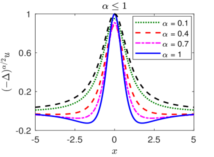
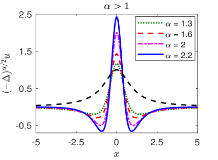
Figure 2: Illustration of function $(-\Delta)^{\frac{\alpha}{2}}(1+x^{2})^{-1}$ for various $\alpha$. For easy comparison, the function $u(x)=(1+x^{2})^{-1}$ is also presented by black dashed lines.

Fig. 2 illustrates function $(-\Delta)^{\frac{\alpha}{2}}u$ for various $\alpha$. It shows that function $(-\Delta)^{\frac{\alpha}{2}}u$ approaches to $u$ as $\alpha\to 0$. The nonlocal effects become stronger for smaller $\alpha$, and particularly we find that $(-\Delta)^{\frac{\alpha}{2}}u(x)\leq u(x)$ for any $x\in{\mathbb{R}}$ if $\alpha\leq 1$. For $\alpha>2$ but $\frac{\alpha}{2}\notin{\mathbb{N}}$, the operator $(-\Delta)^{\frac{\alpha}{2}}$ remains nonlocal, which is beyond the scope of our study.

Table 1 presents the RMS errors of our method in approximating $(-\Delta)^{\frac{\alpha}{2}}u$ on domain $\Omega=(-2,2)$. Here, we take the shape parameter $\varepsilon=2$. The center and test points are chosen to be uniformly distributed on $[-2,2]$. We remark that our method is flexible in choosing center and test points, but the “best” shape parameter might change according to this choice. For example, our studies show that using the Chebyshev points as RBF center and test points can give the similar numerical accuracy as in Table 1, if a larger shape parameter is used. Note that the optimal choice of shape parameter and center and test points of RBF-based methods is still an open research topic [36, 21], and we will leave it for our future study [45].

$\bar{N}$	$\alpha=0.4$	$\alpha=1$	$\alpha=1.6$	$\alpha=2$	$\mathcal{K}$
9	1.957E-3	2.177E-2	8.091E-2	1.941E-1	5.431
17	8.442E-4	4.009E-3	2.230E-2	8.116E-2	5.079E3
33	1.010E-6	7.856E-6	7.732E-5	4.949E-4	2.369E14
65	2.220E-9	1.486E-8	1.832E-7	1.514E-6	2.350E17

Table 1: Numerical errors $\|e_{\Delta}\|_{\rm rms}$ and condition number ${\mathcal{K}}$ in approximating $(-\Delta)^{\frac{\alpha}{2}}u$ for $x\in(-2,2)$, where the shape parameter $\varepsilon=2$ and the exact solution is given in (3.1).

Table 1 shows that our method yields a good approximation to $(-\Delta)^{\frac{\alpha}{2}}u$ even with a small number of points $\bar{N}$. Comparing the errors of different $\alpha$, we find that the larger the exponent $\alpha$, the bigger the numerical errors, but a spectral accuracy is achieved for any $\alpha\in(0,2]$. The condition number ${\mathcal{K}}$ of the linear system increases with the number of points $\bar{N}$, which may lead to an ill-conditioned system if $\bar{N}$ is too big. The ill-conditioning is one issue of methods with infinitely differentiable RBFs, and so far different strategies have been developed to improve or control it (see e.g. [28] and references therein). Recently, new algorithms based on expansion of RBFs have been also proposed in [20, 25, 30] to tackle the ill-conditioning issues. However, the expansion of Gaussian RBFs destroys the property in Lemma 2.1 and thus fails to work for our method. In practical simulations, we can control the condition number to ${\mathcal{O}}(10^{13})\sim{\mathcal{O}}(10^{17})$ via adjusting the shape parameter $\varepsilon$ so as to obtain the best accuracy. Furthermore, multi-precision toolboxes and domain decompositions are also recommended in the literature [42, 28, 43], if higher accuracy is demanded.

As discussed previously, our method of approximating the classical and fractional Laplacians are the same, where extra efforts are required in the fractional cases to evaluate the integrals over the domain ${\mathbb{R}}\backslash(-2,2)$. In Fig. 3, we further demonstrate the pointwise error for $\bar{N}=33$ and $129$. It shows that if $\bar{N}$ is small the maximum error occurs symmetrically around the domain boundary (see Fig. 3 (a)). This is simply because of the lack of points around the domain boundary. Our extensive studies show that including more RBF points around or outside of the boundary could improve the accuracy of approximation, consistent with the observations in [22].

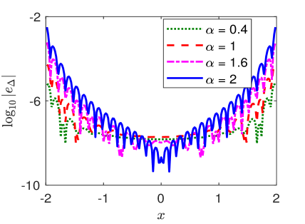
(a) (b)

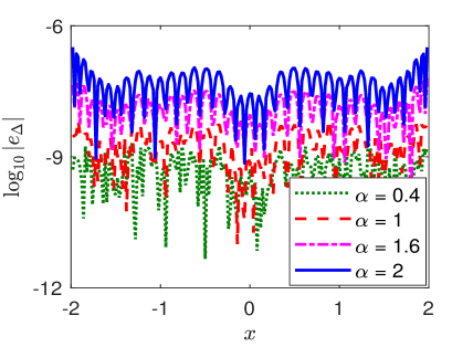
Figure 3: Error distribution in approximating (3.1), where $|e_{\Delta}|=\big{|}(-\Delta)^{\frac{\alpha}{2}}u-(-\Delta)_{h}^{\frac{\alpha}{2}}u\big{|}$. (a) $\bar{N}=33$ and (b) $\bar{N}=129$.

In Fig. 4, we present the numerical approximation of the two-dimensional function $(-\Delta)^{\frac{\alpha}{2}}u$ with $u({\bf x})=\exp[-(x^{2}+y^{2})]\sin(y)$. It shows that the result is symmetric with respect to the $x$-axis, as the function $u$.

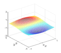
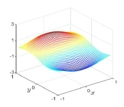
(a) (b) (c)

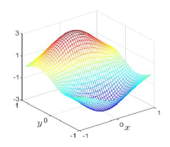
Figure 4: Numerical approximation of $(-\Delta)^{\frac{\alpha}{2}}u$ for two-dimensional function $u({\bf x})=e^{-(x^{2}+y^{2})}\sin(y)$. From (a) to (c): $\alpha=0.6,1.4$, and $2$.

In this case, the exact solution of $(-\Delta)^{\frac{\alpha}{2}}u$ is unknown for $\alpha<2$, but if $\alpha=2$ we have the analytical result:

$$-\Delta u({\bf x})=e^{-(x^{2}+y^{2})}\Big{[}\sin(y)\big{(}4x^{2}+4y^{2}-5\big{)}-4y\cos(y)\Big{]},\qquad\mbox{for}\ {\bf x}\in{\mathbb{R}}^{2}.$$

For $\alpha=2$, our approximate results agree well with their exact solutions (see Fig. 4 (c)). Furthermore, we compare our method with the finite difference method in Table 2, where the RBF center points are taken to be the same as the finite difference grid points. It shows that our method provides a more accurate approximation with the same number of points $\bar{N}$. Moreover, the geometric flexibility and easy implementation make our method more advantageous in high dimensions.

$\bar{N}$	$4^{2}$	$5^{2}$	$6^{2}$	$7^{2}$
FDM	1.046E-2	5.493E-3	3.388E-3	2.299E-3
RBF	3.094E-3	5.479E-5	5.818E-7	4.010E-9

Table 2: Numerical errors $\|e_{\Delta}\|_{\rm rms}$ of the finite difference method (FDM) and our method (RBF) with $\varepsilon=1$ in approximating function $-\Delta u$ on $(-1,1)^{2}$, where $u({\bf x})=e^{-(x^{2}+y^{2})}\sin(y)$.

3.2 Compactly supported functions

In the following, we approximate the Laplacian of compactly supported functions which are often studied in the field of fractional calculus. Consider function $u(x)=x(1-x^{2})^{p}_{+}$ for $x\in{\mathbb{R}}$, which has compact support on $(-1,1)$ and is always zero for $x\notin(-1,1)$. For $p>-1$, there is the exact solution [15]:

$$(-\Delta)^{\frac{\alpha}{2}}u(x)=\frac{2^{\alpha}(\alpha+1)\Gamma((1+\alpha)/2)\Gamma(p+1)}{\sqrt{\pi}\,\Gamma(p+1-\alpha/2)}\,_{2}F_{1}\Big{(}\frac{\alpha+3}{2},\,-p+\frac{\alpha}{2};\,\frac{3}{2};\,x^{2}\Big{)}x,\quad\mbox{for \ $|x|<1$}.$$ (3.2)

It shows in [15] that the exact solution (3.2) holds for $\alpha\in(0,2)$, but we find that it is also valid for $\alpha=2m$ with $m\in{\mathbb{N}}$.

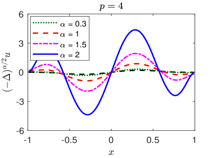
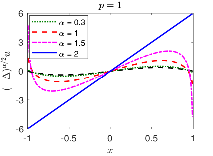
Figure 5: Illustration of function $(-\Delta)^{\frac{\alpha}{2}}\big{[}x(1-x^{2})^{p}_{+}\big{]}$ for different $p$ and $\alpha$. For easy comparison, the function $u(x)=x(1-x^{2})^{p}_{+}$ is also presented by black dashed lines.

It is easy to see that the differentiability of function $u$ at $x=\pm 1$ increases as $p>0$ increases. Fig. 5 compares the solution behavior of $(-\Delta)^{\frac{\alpha}{2}}\big{[}x(1-x^{2})^{p}_{+}\big{]}$ for different $p$ and $\alpha$. It shows that for $p=1$, the results become much sharper around the boundary as $\alpha<2$ increases, which makes the accurate approximation more challenging for low-order methods.

Table 3 presents the RMS errors for cases of $p=4$ and $p=1$, where the RBF center and test points are chosen uniformly on $[-1,1]$ and the shape parameter $\varepsilon=4$. The function $(-\Delta)^{\frac{\alpha}{2}}u$ is approximated following the same process as in Section 3.1, except the boundary conditions considered here are $g(x)=0$ for $x\in{\mathbb{R}}\backslash(-1,1)$. It shows that our method provides a good approximation to $(-\Delta)^{\frac{\alpha}{2}}u$ for both $\alpha=2$ and $\alpha<2$.

$p=4$					$p=1$
$\alpha=0.3$	$\alpha=1$	$\alpha=1.5$	$\alpha=2$	$\bar{N}$	$\alpha=0.3$	$\alpha=1$	$\alpha=1.5$	$\alpha=2$
1.208E-1	4.521E-1	1.2041	3.2937	5	1.725E-1	6.789E-1	2.0617	6.5544
1.456E-3	9.267E-3	3.709E-2	1.539E-1	9	3.423E-2	1.993E-1	7.551E-1	2.9834
1.266E-4	1.169E-3	5.867E-3	2.963E-2	17	3.519E-3	3.159E-2	1.551E-1	7.596E-1
6.636E-7	1.389E-5	1.096E-4	8.462E-4	33	3.074E-6	6.261E-5	4.905E-4	3.777E-3
4.251E-9	4.174E-8	2.793E-7	2.029E-6	65	5.917E-9	5.736E-8	3.803E-7	2.720E-6

Table 3: Numerical errors $\|e_{\Delta}\|_{\rm rms}$ in approximating $(-\Delta)^{\frac{\alpha}{2}}u$ for $x\in(-1,1)$, where the shape parameter $\varepsilon=4$ and the exact solution is given in (3.2).

The larger the exponent $\alpha$, the bigger the numerical errors, similar observation to that from Table 1. Our studies show that the numerical errors are symmetric with respect to $x=0$. Compared to the finite difference methods in [10, 13], the proposed method has significantly smaller errors with the same number of points (see Fig. 6).

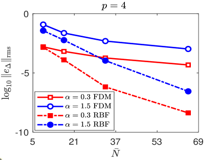
(a) (b)

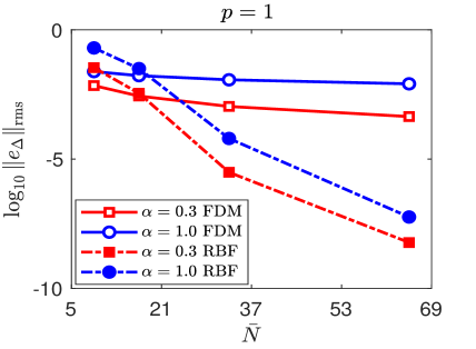
Figure 6: Comparison of numerical errors from our method with $\varepsilon=4$ and the finite difference method in approximating $(-\Delta)^{\frac{\alpha}{2}}\big{[}x(1-x^{2})^{p}_{+}\big{]}$ for $x\in(-1,1)$.

Moreover, the finite difference method fails to converge when $p=1$ and $1<\alpha<2$, since the function $u$ in this case does not satisfy the consistency condition as discussed in [13, 14]. In contrast to it, our method achieves a spectral accuracy for both $p=1$ and $4$.

In Fig. 7, we further study the numerical errors for different shape parameters, where the number of points $\bar{N}=33$ is fixed. We find that the dependence of numerical errors on the shape parameter are qualitatively the same for different $\alpha$ and $p$.

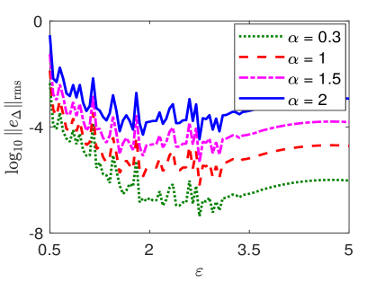
(a) (b)

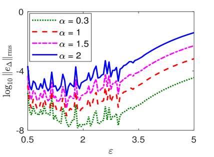
Figure 7: Numerical errors versus shape parameters in approximating the function in (3.2), where the number of points $\bar{N}=33$. (a) $p=4$; (b) $p=1$.

To obtain good accuracy, one should choose the shape parameter neither too small nor too large. The optimal shape parameter might exist and depend not only on the choice RBF points but also on function $u$ and exponent $\alpha$. In Fig. 7, for example, the optimal shape parameter occurs around $2.8$ for $p=4$, while $1.8$ for $p=1$. How to find the optimal shape parameter remains an active research topic in the field of RBF-related methods, and we will leave it for our future research.

4 Solutions of classical and fractional PDEs

In this section, we test the performance of our method in solving both classical and fractional PDEs. So far, most existing numerical methods for fractional PDEs with the integral fractional Laplacian are incompatible with those for their classical counterparts, due to different formulations of the Laplace operators as well as the boundary conditions. For example, the weak formulation of the classical and fractional Poisson equations are significantly different when using finite element methods. Consequently, numerical schemes and computer codes have to be developed separately for the classical and fractional problems. One important merit of our method is to solve both the classical and fractional problems in a single scheme, owing to the unified Laplace formulation of the Gaussian RBFs in Lemmas 2.1 and 2.2. We will further demonstrate this and other advantages of our method in this section. To quantify its performance, we define the RMS error in solution $u$ as:

$$\|e_{u}\|_{\rm rms}=\bigg{(}\frac{1}{M}\sum_{j=1}^{M}\big{|}u_{j}-u_{j}^{h}\big{|}^{2}\bigg{)}^{1/2},$$

where $M$ denotes the number of interpolation points on $\Omega$, and $u_{j}$ and $u_{j}^{h}$, respectively, represent the exact and numerical solutions at point ${\bf x}_{j}\in{\Omega}$.

4.1 One-dimensional Poisson problems

In this case, we take $d=1$ in (2.5)–(2.6) and choose the domain $\Omega=(-1,1)$. We study a benchmark fractional Poisson problem in [10, 40, 2], i.e., choosing

$$f(x)=\frac{2^{\alpha}\Gamma(\frac{\alpha+1}{2})\Gamma(s+1+\frac{\alpha}{2})}{\sqrt{\pi}\Gamma(s+1)}\,_{2}F_{1}\Big{(}\frac{\alpha+1}{2},-s;\,\frac{1}{2};\,x^{2}\Big{)}, \mbox{for}\ x\in\Omega,\qquad$$ (4.1)

$$g(x)\equiv 0, \mbox{for}\ x\in\Upsilon,$$ (4.2)

for $s\in{\mathbb{N}}^{0}$. Noticing the definition of $\Upsilon$, (4.2) implies that the two-point zero boundary conditions at $x=\pm 1$ are imposed for the classical problem with $\alpha=2$, while the extended homogeneous Dirichlet boundary conditions are considered for $\alpha<2$. The exact solution of the Poisson equation with (4.1)–(4.2) is given by $u(x)=(1-x^{2})_{+}^{s+\frac{\alpha}{2}}$ for any $\alpha\in(0,2]$. It is evident that the larger the value of $s$, the better the regularity of solution $u$ up to the boundary.

Table 4 presents the RMS errors $\|e_{u}\|_{\rm rms}$ when different $s$ are chosen in (4.1). In our simulations, the center and test points are taken to be uniformly distributed on $[-1,1]$, and the shape parameter $\varepsilon=4.5$ is used. From Table 4, we find that numerical errors depend on the solution regularity and exponent $\alpha$.

$s=3$					$s=0$
$\alpha=0.6$	$\alpha=1$	$\alpha=1.5$	$\alpha=2$	$\bar{N}$	$\alpha=0.6$	$\alpha=1$	$\alpha=1.5$	$\alpha=2$
3.262E-1	4.134E-1	4.791E-1	5.074E-1	$5$	5.863E-1	6.539E-1	6.922E-1	6.952E-1
5.052E-3	1.308E-2	4.263E-2	1.166E-1	$9$	1.627E-1	1.357E-1	1.437E-1	2.098E-1
1.147E-4	1.648E-4	2.553E-4	3.750E-4	$17$	7.746E-2	5.225E-2	3.405E-2	1.607E-2
3.120E-7	2.909E-6	1.174E-5	2.383E-5	$33$	3.265E-2	1.867E-2	9.485E-3	3.193E-4
8.147E-8	1.719E-7	2.288E-7	1.462E-6	$65$	1.631E-2	8.538E-3	3.966E-3	3.014E-6

Table 4: Numerical errors $\|e_{u}\|_{\rm rms}$ in solving the 1D Poisson problem with $f$ and $g$ defined in (4.1)–(4.2), where the shape parameter $\varepsilon=4.5$.

If the solution $u$ is smooth enough up to the boundary (e.g., $s=3$), the numerical errors decrease with a spectral rate as the number of RBF points increases. Moreover, our numerical errors are much smaller than those computed from finite difference method [10, Tables 4–5] with the same number of points. While $s=0$, the solution of the fractional Poisson problem has low regularity around the boundary, which negatively affects the accuracy of our method. Consequently, the numerical errors of $s=0$ are much larger than those of $s=3$ for any $\alpha\in(0,2)$. However, the effect of $s$ on the solution of the classical problem (i.e., $\alpha=2$) is less significant, as the classical Laplacian is a local operator. For both $s=0$ and $3$, the numerical errors are generally larger around the two boundary points $x=\pm 1$ (see Fig. 8). It implies that including more points around the boundary might improve the accuracy of our method.

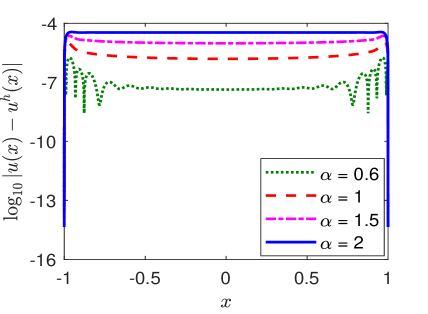
(a) (b)

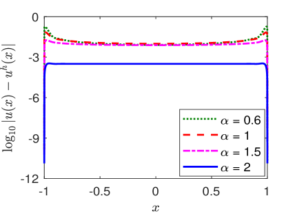
Figure 8: Numerical errors in solving the 1D Poisson problem with $f$ and $g$ defined in (4.1)–(4.2), where we use $\varepsilon=4.5$ and $\bar{N}=33$ in our simulations. (a) $s=3$; (b) $s=0$.

As discussed previously, the shape parameter $\varepsilon$ plays an important role in the accuracy of RBF-based methods. To study it, we compare the numerical errors of different shape parameters in Fig. 9. It shows that the optimal shape parameter depends not only on exponent $\alpha$ but also on solution regularity. For $s=3$, large numerical errors are found if the shape parameter is too small or too big.

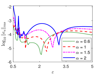
(a) (b)

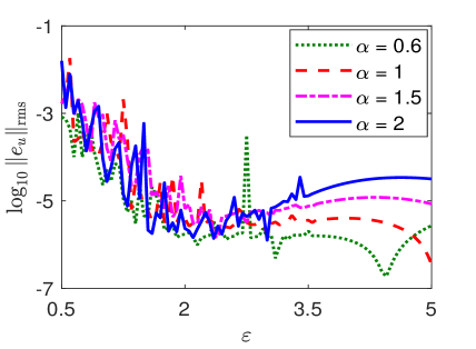
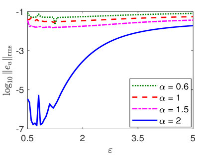
(c) (d)

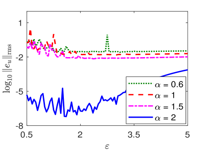
Figure 9: Numerical errors versus shape parameters in solving the 1D Poisson problem with $f$ and $g$ in (4.1)–(4.2). (a) $\bar{N}=17,s=3$; (b) $\bar{N}=33,s=3$; (c) $\bar{N}=17,s=0$; (d) $\bar{N}=33,s=0$.

However, numerical errors for $s=0$ and $\alpha<2$ become almost insensitive to the shape parameter (see Fig. 9 (c) and (d)), suggesting that the solution regularity caps the numerical errors in this case. Moreover, the dependence of numerical errors on the shape parameter becomes more complicated when the number of RBF center points increases, and multiple optimal shape parameters might occur; (cf. Fig. 9 (a) and (b)). We will leave the investigation of optimal shape parameters in solving nonlocal problems as our future research.

Next, we compare our method with the recently proposed pseudospectral method in [40], where the benchmark fractional Poisson problem with $s=0$ was studied. The method in [40] is different from ours mainly in the following aspects:

• It applies the extended Dirichlet boundary conditions to the pseudo-differential form of the fractional Laplacian in (1.1). To this end, this method requires a much larger computational domain than the physical domain $\Omega$. For instance, a computational domain of $[-8,8]$ was taken in solving the Poisson problem on $\Omega=(-1,1)$; see [40, Section 4.2]. This significantly increases the computational cost and storage requirement as more points are demanded in their computations. Fig. 10 (a) compares our numerical errors with those in [40, Table 2] in solving the 1D fractional Poisson problem with $s=0$, where the uniform distance between center points is denoted as $h$. Numerical errors of these two methods are comparable, but the method in [40] used 8 times more points than ours due to its larger computational domain.

  (a) (b)

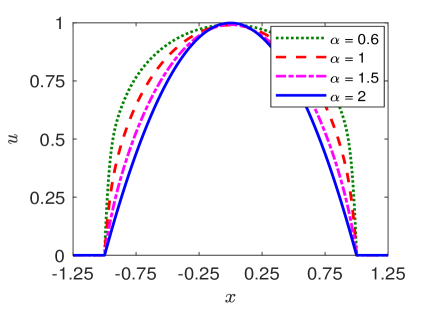
  Figure 10: (a) Comparison of our numerical errors (dashed line) with those in [40, Table 2] (solid line) in solving 1D Poisson problem with $s=0$. (b) Numerical solution of the 1D Poisson problem with $s=0$, showing no Gibbs phenomenon of our method, where the shape parameter $\varepsilon=4.3$.

• Even though a larger computational domain is adopted, it has difficulties to handle the exact boundary conditions over $\Omega^{c}$. In fact, the boundary conditions only on a small region $\omega\subset\Omega^{c}$ is considered in their method; see more discussion in Remark 2.1. Consequently, as pointed out in [40, Figs. 2 and 3], the Gibbs phenomenon was observed near the boundary points $x=\pm 1$, and large numerical errors were found outside of the domain $[-1,1]$. In contrast, our method is free of these issues (see Fig. 10 (b)), as it exactly utilizes the boundary conditions and avoids the RBF approximation on ${\mathbb{R}}\backslash\bar{\Omega}$.

• Different from ours, the method in [40] uses the compactly supported Wendland RBFs as the basis function. Since the fractional Laplacian of Wendland RBFs is unknown, numerical quadrature rules are required for their approximation. This not only complicates the practical implementation of this method but hinders its generalization to problems with the classical Laplacian.

4.2 Two-dimensional Poisson problems

Our meshfree method can easily handle complex geometry, and its computational complexity is independent of dimension $d\geq 1$. In this section, we will study its performance in solving the two-dimensional Poisson problem (2.5)–(2.6) on both regular and irregular domains.

4.2.1 Regular domain

Here, we consider the two-dimensional Poisson problem (2.5)–(2.6) on a unit disk domain, i.e., $\Omega=\{{\bf x}\in{\mathbb{R}}^{2}\,|\,|{\bf x}|<1\}$. We choose function $f({\bf x})\equiv 1$ for ${\bf x}\in\Omega$, and homogeneous Dirichlet boundary conditions $g({\bf x})\equiv 0$ for ${\bf x}\in\Upsilon$. In this case, the exact solution is given by

$$u({\bf x})=2^{-\alpha}\Big{(}\Gamma(1+\frac{\alpha}{2})\Big{)}^{-2}\big{(}1-|{\bf x}|^{2}\big{)}^{\frac{\alpha}{2}},\qquad\mbox{for}\ \ {\bf x}\in\Omega,\quad\alpha\in(0,2].$$

In our simulations, we choose the RBF center and test points radially distributed on the disk domain $\bar{\Omega}$. Choose an integer $n\geq 1$, and define the sets

$${\mathcal{S}}_{\bar{\Omega}}^{c}={\mathcal{S}}_{\bar{\Omega}}^{t}=\bigg{\{}\frac{l}{n}\Big{(}\cos\big{(}2j\pi/(n+1)\big{)},\ \sin\big{(}2j\pi/(n+1)\big{)}\bigg{)},\ \ \mbox{for}\ 0\leq l\leq n,\ 0\leq j\leq n\Big{\}}.$$

that is, the total number of points is $\bar{N}=n(n+1)+1$ with $n$ radial layers.

In this example, the solution has low regularity up to the boundary, i.e. $u\in C^{0,\frac{\alpha}{2}}(\bar{\Omega})$ [13, 15, 2]. The smaller the exponent $\alpha$, the less smooth the solution near boundaries; see Fig. 11 for numerical solution of $\alpha=0.6,1.5$ and $2$. Moreover, the solution becomes much flatter as $\alpha$ increases.

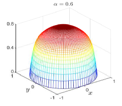
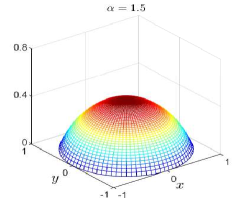
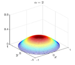
Figure 11: Numerical solution of the Poisson problem on a unit disk domain.

Table 5 presents numerical errors $\|e_{u}\|_{\rm rms}$ for different $n$, where we take the shape parameter $\varepsilon=2$. It shows that as the number of points increases, the numerical errors decrease with a spectral rate for $\alpha=2$. While $\alpha<2$, the solution regularity dominates the problem, and numerical errors decrease slowly, which is similar to the observations in Table 4 for $s=0$.

$n$	$\alpha=0.6$	$\alpha=1$	$\alpha=1.5$	$\alpha=2$
$3$	1.360E-1	8.187E-2	3.817E-2	1.211E-2
$4$	9.802E-2	5.640E-2	2.459E-2	5.924E-3
$5$	7.471E-2	4.130E-2	1.667E-2	2.488E-3
$6$	5.925E-2	3.178E-2	1.204E-2	9.059E-4
$7$	4.844E-2	2.544E-2	9.229E-3	2.803E-4

Table 5: Numerical errors $\|e_{u}\|_{\rm rms}$ in solving the Poisson problem on a unit disk domain, where the shape parameter $\varepsilon=2$.

Fig. 12 further shows the pointwise errors for $\alpha=1$. We find that numerical errors are radially symmetric and the maximum error is found around the domain boundary. This suggests that the local refinement (including more points around boundary) might improve the accuracy of this problem. Our extensive studies show that numerical errors are considerably smaller if the solution is smoother around boundary.

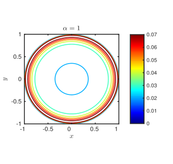
(a) (b)

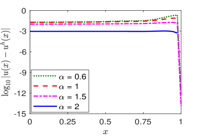
Figure 12: Pointwise numerical errors in solving the Poisson problem on a unit disk domain, where $\alpha=1$ and $y=0$ is fixed in (b).

Compared to other methods, the geometric flexibility enables our method to solve this problem with much less computational efforts. For instance of $\alpha=1$, our method can achieve the accuracy of ${\mathcal{O}}(10^{-2})$ with the total number of points $\bar{N}\approx 10$, but the Wendland RBF method requires at least 400 points due to its larger computational domain (see [40, Table 4]). On the other hand, finite element methods (FEM) are also flexible of domain geometry, but they are mesh-based local approximation methods. The results in [6] show that to achieve the same accuracy, much larger number of unknowns are introduced by FEMs; see [6, Table1]. Moreover, the nonlocality and singularity of the fractional Laplacian makes assembling the stiffness matrix extremely challenging for FEMs [1, 6].

4.2.2 Irregular domain

In this section, we solve the two-dimensional Poisson problem (2.5)–(2.6) on an irregular domain $\Omega=\big{\{}{\bf x}\,|\,{\bf x}\in(-1,1)^{2}\ {\rm and}\ |{\bf x}|>0.5\big{\}}$, i.e. a two-dimensional domain confined between a unit square and a circle with radius $r=0.5$. We will consider an inhomogeneous Dirichlet boundary condition and choose

$$f({\bf x})=\Gamma(2+\alpha)\,_{2}F_{1}\Big{(}\frac{2+\alpha}{2},\frac{3+\alpha}{2};1;-|{\bf x}|^{2}\Big{)}, \quad\mbox{for}\ \ {\bf x}\in\Omega,\qquad$$

$$g({\bf x})=\sqrt{(1+|{\bf x}|^{2})^{-3}}, \quad\mbox{for}\ \ {\bf x}\in\Upsilon.$$

In this case, the exact solution of the Poisson problem can be constructed as $u({\bf x})=\sqrt{(1+|{\bf x}|^{2})^{-3}}$ for ${\bf x}\in{\mathbb{R}}^{2}$ and $\alpha\in(0,2]$.

In our simulations, we take the shape parameter $\varepsilon=1.5$. The test points are chosen to be the same as center points. To this end, we first choose a set of points radially distributed on an annulus for $0.5\leq|{\bf x}|\leq 1$, i.e., for $n\in{\mathbb{N}}$

$$\hat{\mathcal{S}}=\bigg{\{}\Big{(}\frac{1}{2}+\frac{l}{2n}\Big{)}\Big{(}\cos\big{(}j\pi/2n\big{)},\ \sin\big{(}j\pi/2n\big{)}\bigg{)},\ \ \mbox{for}\ 0\leq l\leq n,\ 1\leq j\leq 4n\Big{\}}.$$

Then we map the points in $\hat{\mathcal{S}}$ to domain $\Omega$ using the elliptic grid mapping [23], i.e., letting

$$x_{i}=\frac{1}{2}\bigg{(}\sqrt{2+\hat{x}_{i}^{2}-\hat{y}_{i}^{2}+2\sqrt{2}\hat{x}_{i}}-\sqrt{2+\hat{x}_{i}^{2}-\hat{y}_{i}^{2}-2\sqrt{2}\hat{x}_{i}}\bigg{)},$$

$$y_{i}=\frac{1}{2}\bigg{(}\sqrt{2-\hat{x}_{i}^{2}+\hat{y}_{i}^{2}+2\sqrt{2}\hat{y}_{i}}-\sqrt{2-\hat{x}_{i}^{2}+\hat{y}_{i}^{2}-2\sqrt{2}\hat{y}_{i}}\bigg{)},$$

for $(\hat{x}_{i},\hat{y}_{i})\in\hat{\mathcal{S}}$. That is, the total number of points is $\bar{N}=4n(n+1)$.

Fig. 13 shows the numerical solution and pointwise errors for $\alpha=1.5$.

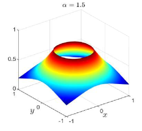
(a) (b)

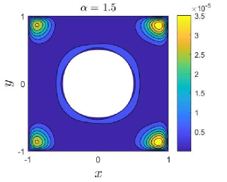
Figure 13: Numerical solution (a) and numerical errors (b) in solving the two-dimensional Poisson problem on an irregular domain, where we choose $n=5$ in our simulations.

We find that numerical errors reach the maximum at four corners of the domain, but overall they are small even with the number of points $\bar{N}=24$. Table 6 further demonstrates the numerical errors $\|e_{u}\|_{\rm rms}$ and condition number ${\mathcal{K}}$ of the linear system for various $\alpha$.

	$\alpha=0.6$		$\alpha=1$		$\alpha=1.5$		$\alpha=2$
n	$\|e_{u}\|_{\rm rms}$	$\mathcal{K}$	$\|e_{u}\|_{\rm rms}$	$\mathcal{K}$	$\|e_{u}\|_{\rm rms}$	$\mathcal{K}$	$\|e_{u}\|_{\rm rms}$	$\mathcal{K}$
$2$	1.635E-3	2.313E7	1.772E-3	3.143E7	2.044E-3	4.694E7	2.503E-3	6.955E7
$3$	2.983E-4	3.50E11	3.958E-4	5.69E11	6.156E-4	1.03E12	1.006E-3	1.51E12
$4$	8.118E-5	1.69E16	9.821E-5	2.48E16	1.554E-4	4.58E16	9.821E-5	4.41E16

Table 6: Numerical errors $\|e_{u}\|_{\rm rms}$ and condition number ${\mathcal{K}}$ in solving the two-dimensional Poisson problem on an irregular domain, where the shape parameter $\varepsilon=1.5$.

Compared to the results in Table 5, numerical errors reduce much faster as the number of points increases, since the solution in this case are infinitely differentiable on ${\mathbb{R}}^{2}$. With $\bar{N}$ further increasing, the system may become ill-conditioned and affect the simulation errors. Recently, multi-precision toolboxes and domain decompositions have been proposed to resolve this issue; see [28, 42, 43] and references therein for more discussion.

4.3 Diffusion problems

In this section, we further study the performance of our method in solving time-dependent problems. To this end, we consider the following diffusion problem with nonhomogeneous Dirichlet boundary conditions:

$$\partial_{t}u({\bf x},t)=-(-\Delta)^{\frac{\alpha}{2}}u+f({\bf x},t), \mbox{for}\ \ {\bf x}\in\Omega=(-1,1)^{2},\quad t>0,\qquad$$ (4.3)

$$u({\bf x},t)=t(1+0.5|{\bf x}|^{2})^{-\frac{3}{2}}, \mbox{for}\ \ {\bf x}\in\Upsilon,\quad t\geq 0,$$ (4.4)

$$u({\bf x},0)=0, \mbox{for}\ \ {\bf x}\in{\mathbb{R}}^{2}.$$ (4.5)

The source term $f$ is chosen such that the exact solution of (4.3)–(4.5) is given by:

$$u(x,y)=t/\sqrt{\big{(}1+0.5(x^{2}+y^{2})\big{)}^{3}},\qquad\mbox{for}\ \ {\bf x}\in{\mathbb{R}}^{2},\quad t\geq 0.$$ (4.6)

Denote time sequence $t_{n}=n\Delta t$ (for $n=0,1,\ldots$) with time step $\Delta t>0$. Choose the RBF center and test points as uniformly distributed tensor grid points on $[-1,1]^{2}$. We then discretize (4.3) with the Crank–Nicolson method in time and our meshfree method in space and obtain the fully discretized scheme as:

$$\frac{u^{n+1}_{k}-u^{n}_{k}}{\Delta t}=-(-\Delta)_{h}^{\frac{\alpha}{2}}\Big{(}\frac{u_{k}^{n}+u_{k}^{n+1}}{2}\Big{)}+\frac{f({\bf x}_{k},t_{n})+f({\bf x}_{k},t_{n+1})}{2},\quad\mbox{for}\ \ {\bf x}_{k}\in{\mathcal{S}}_{\Omega}^{t},\ \ n=0,1,\ldots,$$ (4.7)

where $(-\Delta)_{h}^{\frac{\alpha}{2}}u_{k}^{n}$ represents the numerical approximation of $(-\Delta)^{\frac{\alpha}{2}}u({\bf x}_{k},t_{n})$ with $u_{k}^{n}$ being the approximation of $u({\bf x}_{k},t_{n})$, i.e.

$$u^{n}_{k}=\sum_{1\leq i\leq\bar{N}}\lambda_{i}^{n}\varphi^{\varepsilon}(|{\bf x}_{k}-{\bf x}_{i}|).$$ (4.8)

At each time step, we will solve for the unknowns $\lambda_{i}^{n+1}$ for $1\leq i\leq\bar{N}$. Simplifying (4.7) and applying (4.8) to boundary points ${\bf x}_{k}\in{\mathcal{S}}_{\partial\Omega}^{t}$, we then obtain our scheme in matrix-vector form:

$$\left(\begin{array}[]{c}\displaystyle B_{N\times\bar{N}}+\frac{\Delta t}{2}A_{N\times\bar{N}}\\ \displaystyle C_{(\bar{N}-N)\times\bar{N}}\end{array}\right)\Lambda_{\bar{N}\times 1}^{n+1}=\left(\begin{array}[]{c}\displaystyle\Big{(}B-\frac{\Delta t}{2}A\Big{)}\Lambda^{n}+\frac{\Delta t}{2}\big{(}{\bf f}^{n}+{\bf f}^{n+1}+{\bf w}^{n}+{\bf w}^{n+1}\big{)}\\ \displaystyle{\bf g}^{n+1}\end{array}\right),$$ (4.13)

for $n=0,1,\ldots$, where we denote $\Lambda_{\bar{N}\times 1}^{n}=\big{(}\lambda_{1}^{n},\cdots,\lambda_{\bar{N}}^{n}\big{)}^{T}$,  ${\bf f}_{N\times 1}^{n}=\big{(}f({\bf x}_{1},t_{n}),\cdots,f({\bf x}_{N},t_{n})\big{)}^{T}$, and ${\bf g}_{(\bar{N}-N)\times 1}^{n}=\big{(}g({\bf x}_{N+1},t_{n}),\cdots,g({\bf x}_{\bar{N}},t_{n})\big{)}^{T}$ with $g$ denoting the boundary condition in (4.4). The vector ${\bf w}_{N\times 1}^{n}=\big{(}w({\bf x}_{1},t_{n}),\cdots,w({\bf x}_{N},t_{n})\big{)}^{T}$ is from the discretization of $(-\Delta)^{\frac{\alpha}{2}}$ in (2.11) with

$$w({\bf x},t)=\zeta_{\alpha}C_{d,\alpha}\int_{\Omega^{c}}\frac{g({\bf y},t)}{|{\bf x}-{\bf y}|^{d+\alpha}}d{\bf y},$$

which reduces to zero if $\alpha=2$ or homogeneous boundary conditions are considered. The matrices $B$ and $C$ are composed of the Gaussian RBFs $\varphi^{\varepsilon}(|{\bf x}_{k}-{\bf x}_{i}|)$, while the entries of matrix $A$ are given by the coefficients of $\lambda_{i}$ in (2.2). All of these matrices remain the same at all time steps.

In our simulations, we take a small time step $\Delta t=0.001$ such that the temporal errors are neglectable in comparison to spatial errors. Fig. 14 shows the time evolution of the solution for $\alpha=1$, which agree well with the exact solution in (4.6).

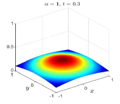
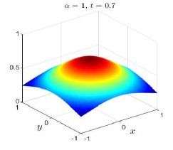
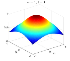
Figure 14: Time evolution of the solution of the diffusion problem (4.3)–(4.5).

Furthermore, we present the numerical errors $\|e_{u}\|_{\rm rms}$ at $t=1$ and the condition number ${\mathcal{K}}$ of the linear system in Fig. 15. It shows that numerical errors decrease with a spectral rate for any $\alpha\in(0,2]$, while the condition number increases quickly as more points are used.

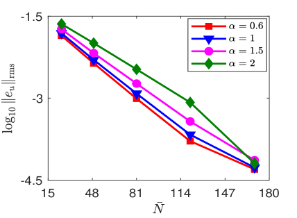
(a) (b)

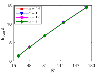
Figure 15: Numerical errors $\|e_{u}\|_{\rm rms}$ at time $t=1$ and condition number ${\mathcal{K}}$ in solving the diffusion problem (4.3)–(4.5), where the shape parameter $\varepsilon=1.9$.

If the number of points $\bar{N}$ is too big, one can adopt the strategies in [42, 28, 43] to avoid the ill-conditioning issue.

5 Summary and discussions

We proposed a novel meshfree pseudospectral method to solve both the classical and fractional PDEs in a unified scheme. Our method takes great advantage of the Laplacian of the Gaussian RBFs and enables us to approximate the classical and fractional Laplacian in a single framework, which is the key merit of our method distinguishing it from other existing methods for fractional PDEs. Extensive numerical experiments were carried out to study the performance of our method in approximating the Dirichlet Laplace operators and solving the classical and fractional PDE problems. Compared to mesh-based methods, our method can easily handle complex geometry and achieve higher accuracy with fewer points. More importantly, our method can solve the $d$-dimensional (for $d\geq 1$) classical and fractional PDEs with a single computer implementation, which could greatly benefit the study of coexistence of normal and anomalous diffusion in recent applications. We compared our method with the recently proposed Wendland RBF method in [40]. In contrast to it, our method exactly incorporates the Dirichlet boundary conditions into the scheme and is free of the Gibbs phenomenon as observed in [40]. Moreover, the method in [40] solves the problem on a computational domain that is much larger than the physical domain $\bar{\Omega}$, and consequently its computational complexity is much larger than ours. Our studies suggested that to obtain good accuracy the shape parameter cannot be too small or too big, and the optimal shape parameter depends on the RBF center points, the exponent $\alpha$, and the solution properties. How to find the optimal shape parameter is still an active research topic in the area of RBF-based methods. We will leave it for our future study, especially in solving nonlocal problems.

Acknowledgements. We acknowledge two anonymous reviewers for their valuable comments that greatly help to improve this manuscript. This work was supported by the US National Science Foundation under Grant Number DMS-1913293 and DMS-1953177.

References

- [1] G. Acosta, F. M. Bersetche, and J. P. Borthagaray. A short FE implementation for a 2d homogeneous Dirichlet problem of a fractional Laplacian. Comput. Math. Appl., 74(4):784–816, 2017.
- [2] G. Acosta and J. P. Borthagaray. A fractional Laplace equation: Regularity of solutions and finite element approximations. SIAM J. Numer. Anal., 55(2):472–495, 2017.
- [3] M. Ainsworth and C. Glusa. Hybrid finite element-spectral method for the fractional Laplacian: Approximation theory and efficient solver. SIAM J. Sci. Comput., 40(4):A2383–A2405, 2018.
- [4] B. Baeumer and M. M. Meerschaert. Tempered stable Lévy motion and transient super-diffusion. J. Comput. Appl. Math., 233(10):2438–2448, 2010.
- [5] S. D. Bond, R. B. Lehoucq, and S. T. Rowe. A Galerkin Radial Basis Function Method for Nonlocal Diffusion. Lect. Notes Comput. Sci. Eng. Springer, 2015.
- [6] A. Bonito, W. Lei, and J. E. Pasciak. Numerical approximation of the integral fractional Laplacian. Numer. Math., 142(2):235–278, 2019.
- [7] W. Chen and G. Pang. A new definition of fractional Laplacian with application to modeling three-dimensional nonlocal heat conduction. J. Comput. Phys., 309:350–367, 2016.
- [8] D. B. Del-Castillo-Negrete, B. Carreras, and V. Lynch. Fractional diffusion in plasma turbulence. Phys. Plasmas, 11(8):3854–3864, 2004.
- [9] M. D’Elia and M. Gunzburger. The fractional Laplacian operator on bounded domains as a special case of the nonlocal diffusion operator. Comput. Math. Appl., 66(7):1245–1260, 2013.
- [10] S. Duo, H. W. van Wyk, and Y. Zhang. A novel and accurate finite difference method for the fractional Laplacian and the fractional Poisson problem. J. Comput. Phys., 355:233–252, 2018.
- [11] S. Duo and Y. Zhang. Computing the ground and first excited states of the fractional Schrödinger equation in an infinite potential well. Commun. Comput. Phys., 18(2):321–350, 2015.
- [12] S. Duo and Y. Zhang. Mass-conservative Fourier spectral methods for solving the fractional nonlinear Schrödinger equation. Comput. Math. with Appl., 71(11):2257–2271, 2016.
- [13] S. Duo and Y. Zhang. Accurate numerical methods for two and three dimensional integral fractional Laplacian with applications. Comput. Methods. Appl. Mech. Eng., 355:639–662, 2019.
- [14] S. Duo and Y. Zhang. Numerical approximations for the tempered fractional Laplacian: Error analysis and applications. J. Sci. Comput., 81(1):569–593, 2019.
- [15] B. Dyda. Fractional calculus for power functions and eigenvalues of the fractional Laplacian. Fract. Calc. Appl. Anal., 15(4):536–555, 2012.
- [16] B. Dyda, A. Kuznetsov, and M. Kwaśnicki. Fractional Laplace operator and Meijer G-function. Constr. Approx., 45(3):427–448, 2017.
- [17] P. W. Egolf and K. Hutter. Nonlinear, Nonlocal and Fractional Turbulence. Graduate Studies in Mathematics. Springer, first edition, 2020.
- [18] B. P. Epps and B. Cushman-Roisin. Turbulence modeling via the fractional Laplacian. arXiv:1909.09943v1, 2019.
- [19] G. E. Fasshauer. Meshfree Approximation Methods with Matlab. World Scientific, first edition, 2007.
- [20] G. E. Fasshauer and M. J. McCourt. Stable evaluation of Gaussian radial basis function interpolants. SIAM J. Sci. Comput., 34(2):A737–A762, 2012.
- [21] G. E. Fasshauer and J. G. Zhang. On choosing “optimal” shape parameters for RBF approximation. Numer. Algorithms, 45(1–4):345–368, 2007.
- [22] A. I. Fedoseyev, M. J. Friedman, and E. J. Kansa. Improved multiquadric method for elliptic partial differential equations via PDE collocation on the boundary. Comput. Math. Appl., 43(3-5):439–455, 2002.
- [23] C. Fong. Analytical methods for squaring the disc. arXiv:1509.06344v4, 2014.
- [24] B. Fornberg and N. Flyer. A Primer on Radial Basis Functions with Applications to the Geosciences. Society for Industrial and Applied Mathematics, Philadelphia, first edition, 2015.
- [25] B. Fornberg, E. Larsson, and N. Flyer. Stable computations with Gaussian radial basis functions. SIAM J. Sci. Comput., 33(2):869–892, 2011.
- [26] B. Fornberg and J. Zuev. The Runge phenomenon and spatially variable shape parameters in RBF interpolation. Comput. Math. Appl., 54(3):379–398, 2007.
- [27] M. Javanainen, H. Hammarén, L. Monticelli, J. Jeon, M. S. Miettinen, H. Martinez-Seara, R. Metzler, and I. Vattulainen. Anomalous and normal diffusion of proteins and lipids in crowded lipid membranes. Faraday Discuss., 161:397–417, 2013.
- [28] E. J. Kansa and P. Holoborodko. On the ill-conditioned nature of RBF strong collocation. Eng. Anal. Bound. Elem., 78:26–30, 2017.
- [29] K. Kirkpatrick and Y. Zhang. Fractional Schrödinger dynamics and decoherence. Physica D, 332:41–54, 2016.
- [30] K. Kormann, C. Lasser, and A. Yurova. Stable interpolation with isotropic and anisotropic gaussians using hermite generating function. SIAM J. Sci. Comput., 41(6):A3839–A3859, 2019.
- [31] M. Kwaśnicki. Ten equivalent definitions of the fractional Laplace operator. Fract. Calc. Appl. Anal., 20(1):7–51, 2017.
- [32] N. S. Landkof. Foundations of Modern Potential Theory. Springer-Verlag, New York-Heidelberg, 1972.
- [33] N. Laskin. Fractional quantum mechanics and Lévy path integrals. Phys. Lett. A, 268(4–6):298–305, 2000.
- [34] R. B. Lehoucq and S. T. Rowe. A radial basis function Galerkin method for inhomogeneous nonlocal diffusion. Comput. Methods Appl. Mech. Eng., 299:366–380, 2016.
- [35] R. L. Magin. Fractional calculus models of complex dynamics in biological tissues. Comput. Math. Appl., 59(5):1586–1593, 2010.
- [36] Z. Majdisova and V. Skala. Radial basis function approximations: Comparison and applications. Appl. Math. Model., 51:728–743, 2017.
- [37] G. Pang, W. Chen, and Z. Fu. Space-fractional advection-dispersion equations by the Kansa method. J. Comput. Phys., 293:280–296, 2015.
- [38] C. Piret and E. Hanert. A radial basis functions method for fractional diffusion equations. J. Comput. Phys., 238:71–81, 2013.
- [39] A. P. Prudnikov, Yu. A. Brychkov, and O. I. Marichev. Integrals and series. Vol. 3. Gordon and Breach Science Publishers, New York, 1990. More special functions, Translated from the Russian by G. G. Gould.
- [40] J. A. Rosenfeld, S. A. Rosenfeld, and W. E. Dixon. A mesh-free pseudospectral approach to estimating the fractional Laplacian via radial basis functions. J. Comput. Phys., 390:306–322, 2019.
- [41] S. G. Samko, A. A. Kilbas, and O. I. Marichev. Fractional Integrals and Derivatives. Gordon and Breach Science Publishers, Yverdon, 1993.
- [42] S. A. Sarra. Radial basis function approximation methods with extended precision floating point arithmetic. Eng. Anal. Bound. Elem., 35(1):68–76, 2011.
- [43] S. A. Sarra and S. Cogar. An examination of evaluation algorithms for the RBF method. Eng. Anal. Bound. Elem., 75:36–45, 2017.
- [44] T. Tang, L. Wang, H. Yuan, and T. Zhou. Rational spectral methods for PDEs involving fractional Laplacian in unbounded domains. SIAM J. Sci. Comput., 42(2):A585–A611, 2020.
- [45] Y. Wu and Y. Zhang. A universal solution scheme for fractional and classical pdes. preprint, 2020.
- [46] S. Zafarghandi, Fahimeh, and M. Maryam. Numerical approximations for the Riesz space fractional advection-dispersion equations via radial basis functions. Appl. Numer. Math., 144:59–82, 2019.
- [47] Y. Zhang, M. Meerschaert, and A. Packman. Linking fluvial bed sediment transport across scales. Geophys. Res. Lett., 39:L20404, 2012.
- [48] Z. Zhang. Error estimates of spectral Galerkin methods for a linear fractional reaction-diffusion equation. J. Sci. Comput., 78(2):1087–1110, 2019.
- [49] W. Zhao, Y. Hon, and M. Stoll. Localized radial basis functions-based pseudo-spectral method (LRBF-PSM) for nonlocal diffusion problems. Comput. Math. Appl., 75(5):1685–1704, 2018.