Effects of Electron-Vibrational Interaction in Polariton Luminescence: Non-Markovian Fano Resonances and Hot Luminescence

Abstract

We have developed a non-Markovian theory of the polariton luminescence taking the molecular vibrations into account. The calculations were made in the polariton basis. We have shown that the frequency shift and the polariton spectral lines broadening strongly depend on the frequency-dependent exciton contribution to the polariton. In the single-mode microcavity our non-Markovian theory predicts the Fano resonances in the polariton luminescence, and also narrowing of the spectral lines with the increase of the total number of molecules in the case of the intramolecular nature of the low frequency vibrations. The theory enables us to consider a non-equilibrium (hot) exciton-polariton luminescence similar to the hot luminescence of molecules and crystals. This opens a way for its observation in organic-based nanodevices.

1 Introduction

In recent years the Frenkel exciton polaritons (EPs) in organic materials such as dye molecules^{1, 2}, polymers and biological nanostructures³, have attracted considerable interest in the context of the polariton chemistry^{4, 5, 6} and due to their property to form the EP Bose-Einstein condensate⁷ leading to the macroscopic coherence and superfluidity⁸. The process of condensation opens a practical possibility for manufacturing of the low threshold polariton lasers with conventional nanosecond excitation³.

The concept of EPs suggests the presence of the strong interaction between light and matter^{9, 10, 11}. This effect becomes well pronounced especially in organic dyes. The oscillator strength of the organic dye molecules is known to be large compared to inorganic semiconductors. This results in a large separation between the lower (L) and upper (U) polariton branches, which can reach values^{1, 12} $\sim 0.5-1eV$.

The absorption spectrum of a large molecule manifests a progression of spectral lines shifted with respect to each other on the frequency of a high-energetic optically active (OA) vibration (a vibrational mode that reorganizes after electronic excitation) $\omega_{0}\approx 1200-1500$ $cm^{-1}$. Polariton absorption of the electron-vibational systems was studied in a microcavity using a model of a single high-frequency (HF) OA vibration with a phenomenological constant decay rate (Markovian relaxation) ¹³; in organic dye nanofibers using a mean-field theory for intermolecular interactions and a realistic non-Markovian model of HF and low frequency (LF) OA molecular vibrations ¹⁴. In a single mode cavity the polariton absorption was investigated in the presence of Brownian dissipation from molecular vibrations ¹⁵, and also in the Langevin approach ^{16, 17}.

The luminescence of EPs attracted attention immediately after introduction of the polariton concept. The clear physical picture of the polariton relaxation formulated for a weak exciton-phonon interaction ¹⁸, however, is not applicable to the molecular systems, where the electron-vibration interactions are strong. In this case, both the interaction with radiation field and the electron-vibrational interaction must be regarded as equally strong, which makes solution of the problem a challenging task ¹⁸. Equilibrium polariton luminescence of molecular electron-vibrational systems in cavity was calculated using numerical solution of coupled equations of motion ¹⁹ or balance equations ²⁰, where the authors took a single HFOA intramolecular vibration into account. They introduced also complex exciton replicas frequencies with an imaginary part describing the phenomenological constant damping rates (Markovian relaxation) ¹³. In a more realistic situation, however, the relaxation of molecular, exciton and polariton systems are essentially non-Markovian ^{21, 22} and cannot be described by means of the constant decay rates, which can only result in the Lorentzian shape spectra. To this end the Brownian dissipation model has been used in Ref.¹⁵. The authors focused on the elastic cavity emission and restricted their consideration onto the specific case, when the polariton spectra linewidth is the mean of the cavity and the molecular linewidth, under the resonance condition, i.e. when the cavity eigenfrequency is in resonance with the molecular excitation transition. However, the luminescence is essentially an inelastic process, where the interaction of the polariton with molecular vibrations should depend on the exciton contribution to the polariton.

In this work we calculate the polariton luminescence, working in the polariton basis and using the non-Markovian theory for the description of the polariton-molecular vibration interactions. We show that the frequency shift and the polariton spectrum broadening strongly depend on the exciton contribution to the polariton, which is a function of frequency. Since the proper description of the Stokes shift is very important for a correct luminescence theory, we adopt here a realistic model, according to which each member of the progression with respect to a HFOA molecular vibrations of the absorption and luminescence molecular spectra is broadened due to the presence of the LFOA vibrations $\{\omega_{\sigma}\}$. The latter makes the main contribution to the Stokes shift in dyes ^{23, 24, 12, 14}.

It is usually believed that the polariton states are formed when the splitting of the upper and the lower polariton branches is larger than the broadening of the molecular resonances. In contrast, our non-Markovian theory demonstrates (i) the main characteristic features of the Fano resonance in the polariton luminescence spectra, which appears due to the interference of the contributions from the upper and lower polariton branches in the regime of small splitting; and (ii) the motional narrowing of the EP luminescence spectrum in the case of the intramolecular nature of the LFOA vibrations with an increase in the number of molecules in the single mode microcavity. In addition (iii), the theory enables us to consider the non-equilibrium (hot) EP luminescence and opens a way for its observation in organic-based nanodevices in analogy with the hot luminescence of molecules and crystals ^{25, 26}.

2 Model Hamiltonian

Consider an ensemble of molecules with two electronic states ($1$ and $2$), which is described by the Hamiltonian

$$H_{0}=\hbar\sum_{m=1}^{\mathcal{N}}\Big{[}(\omega_{el}+\omega_{0}X_{0m}^{2}+\sum\limits_{\sigma}\omega_{\sigma}X_{\sigma m}^{2})b_{m}^{{\dagger}}b_{m}-\omega_{0}X_{0m}(c_{0m}^{{\dagger}}+c_{0m})b_{m}^{{\dagger}}b_{m}\\ -\sum_{\sigma}\omega_{\sigma}X_{\sigma m}(c_{\sigma m}^{{\dagger}}+c_{\sigma m})b_{m}^{{\dagger}}b_{m}+\omega_{0}c_{0m}^{{\dagger}}c_{0m}+\sum\limits_{\sigma}\omega_{\sigma}c_{\sigma m}^{{\dagger}}c_{\sigma m}\Big{]},$$ (1)

where $\omega_{el}$ is the frequency of the transition from the ground state $1$ to the excited electronic state $2$, $\mathcal{N}$ is the number of molecules. Annihilation of the excited state in the molecule $m$ is described by the operator $b_{m}=\left|m1\right\rangle\langle m2|$, and $b_{m}^{{\dagger}}=\left|m2\right\rangle\langle m1|$ describes the excitation in the $m$th molecule. The OA vibrations are accounted by the annihilation and creation operators of the $i$th mode $c_{im}$ and $c_{im}^{{\dagger}}$, respectively. A shift in the equilibrium position of the OA vibration after excitation of the molecule $m$ is described by the quantity $X_{im}$ ($i=0,\sigma$). It is related to the standard Huang-Rhys factor $S_{im}$, e.g. $S_{0m}=X_{0m}^{2}$.

The light-matter interaction in the dipole approximation can be written equivalently in two ways, by using $\mathbf{r\cdot E}$ or $\mathbf{p\cdot A}$ interaction Hamiltonians ²⁷ with $\mathbf{E}$ being the electric field, $\mathbf{A}$ - the vector potential, and $\mathbf{p}$ - the canonical momentum operator. Though both Hamiltonians for the light-matter interaction are related via the gauge transformation and formally equivalent, they can lead to different results ²⁷ and thus have to be used with a care. Since the exciton-polariton problem was first formulated with the aid of the vector potential ^{11, 10} (see also ²⁸), we also stick to the $\mathbf{p\cdot A}$ Hamiltonian. In this case the electromagnetic-field and the light-matter interaction Hamiltonians are

$$H_{ph+int}=\hbar\sum_{\mathbf{q}}\omega_{\mathbf{q}}a_{\mathbf{q}}^{{\dagger}}a_{\mathbf{q}}-\frac{e}{Mc}\sum\limits_{m}\mathbf{A}(\mathbf{r}_{m})\cdot\mathbf{p}(\mathbf{r}_{m}),$$ (2)

with $e$ and $M$ being the electron charge and mass, respectively, $c$ - the light velocity,

$$\mathbf{A}(\mathbf{r}_{m})=\sum_{\mathbf{q,e}_{\mathbf{q}}}\sqrt{\frac{2\pi\hbar c^{2}}{V\omega_{\mathbf{q}}}}\mathbf{e}_{\mathbf{q}}\left[a_{\mathbf{q}}e^{i\mathbf{q\cdot r}_{m}}+H.c.\right],$$ (3)

$$\mathbf{p}(\mathbf{r}_{m})=-\frac{i\mathbf{D}M\omega_{el}}{e}(b_{m}-b_{m}^{{\dagger}})$$ (4)

Here $H.c.$ denotes Hermitian conjugate, $\mathbf{D}$ is the electronic transition dipole moment, $\mathbf{e}_{\mathbf{q}}$ is the unit photon polarization vector, $V$ is the photon quantization volume. In the rotating-wave approximation, Hamiltonian $H_{ph+int}$ can be written as

$$H_{ph+int}=\hbar\sum_{\mathbf{q}}\omega_{\mathbf{q}}a_{\mathbf{q}}^{{\dagger}}a_{\mathbf{q}}\\ -i\hbar\sum\limits_{m}\sum_{\mathbf{q}}\left[\frac{ge^{-i\mathbf{q\cdot r}_{m}}}{\sqrt{\omega_{\mathbf{q}}}}b_{m}a_{\mathbf{q}}^{{\dagger}}-H.c.\right],$$ (5)

using Eqs.(2), (3) and (4). The light-matter interaction parameter $g$ is

$$g=-\omega_{el}\sum_{\mathbf{e}_{\mathbf{q}}}\sqrt{\frac{2\pi}{\hbar V}}(\mathbf{e}_{\mathbf{q}}\cdot\mathbf{D})$$ (6)

Below we consider the LF vibrational subsystem as a classical one, since we assume that $\hbar\omega_{\sigma}\ll k_{B}T$. An optical electronic transition takes place at a fixed nuclear configuration, according to the Franck-Condon principle. Then representing the electron-vibration coupling quantity $\alpha_{m}=\sum_{\sigma}\omega_{\sigma}X_{\sigma m}(c_{\sigma m}^{{\dagger}}+c_{\sigma m})$ can be considered as a perturbation of the electronic transition by nuclear motion. Essentially the LFOA vibrations ²⁹ can be thought of as a random modulation of the electronic transition frequency, such that $\tilde{\omega}_{21}(t)=\omega_{el}+\omega_{st}/2-\alpha_{m}(t)$, where $\omega_{st}=2\sum_{\sigma}\omega_{\sigma}X_{\sigma m}^{2}=\hbar K(0)/(k_{B}T)$ is the contribution of the LFOA vibrations to the Stokes shift of the equilibrium absorption and luminescence spectra, and $\alpha_{m}(t)$ is a random process. In that case $H_{0}$ becomes a stochastic Hamiltonian and can be represented as

$$H_{0}(\alpha)=\hbar\sum\limits_{m}\Big{\{}\big{[}(\omega_{el}+\omega_{st}/2+\omega_{0}X_{0m}^{2}-\alpha_{m})\\ -\omega_{0}X_{0m}(c_{0m}^{{\dagger}}+c_{0m})\big{]}b_{m}^{{\dagger}}b_{m}+\omega_{0}c_{0m}^{{\dagger}}c_{0m}\Big{\}}$$ (7)

We describe the electronic transition relaxation stimulated by LFOA vibrations ^{30, 31, 32} by a one-parametric Gaussian process with $\langle\alpha_{m}(t)\rangle_{1}=0$. In a particular case, this can be a Gauss-Markov process with an exponential correlation function and a characteristic attenuation time $\tau_{\sigma}$, $K_{m}(t)=\langle\alpha_{m}(0)\alpha_{m}(t)\rangle_{1}=K(0)\exp(-|t|/\tau_{\sigma})$, where $\langle\cdot\rangle_{1}$ stands for the trace operation over the reservoir variables in the ground electronic state $1$.

In this work we focus on calculation of the polariton luminescence spectrum, bearing in mind two types of organic dye molecular systems: the H-aggregates of dye molecules and solution of enhanced green fluorescent protein (eGFP). The experimental ³³ and the theoretical¹⁴ results show that the dipole-dipole interaction between the molecules affects more strongly the absorption line-shape of the H-aggregates (due to redistribution of intensities of vibronic transitions related to the HFOA vibration) than their luminescence spectrum. Fast relaxation of the HFOA vibration leads to the fact that only $0-0$ vibronic transition with respect to the HFOA vibration contributes to the polariton luminescence (see below). As for eGFP, the actual fluorophore of FPs is enclosed by a nano-cylinder that consists of eleven $\beta$-sheets ^{34, 3}. This protective shell acts as natural ‘bumper’ and prevents close contact between fluorophores of neighbouring FPs, limiting the intermolecular energy migration even at the highest possible concentration. Thus, as a first approximation, one can exclude the dipole-dipole interactions between molecules from our consideration.

Hamiltonian $H_{0}(\alpha)$ can be diagonalized with respect to the HFOA vibration using unitary Lang-Firsov transformation $\exp(-S)$ ^{35, 36}, where

$$S=\sum\limits_{m}X_{0m}(c_{0m}^{{\dagger}}-c_{0m})b_{m}^{{\dagger}}b_{m}$$ (8)

As a result one get for the transformed Hamiltonian $\tilde{H}_{0}(\alpha)=\exp(-S)H_{0}(\alpha)\exp(S)$

$$\tilde{H}_{0}(\alpha)=\hbar\sum\limits_{m}[(\omega_{el}+\omega_{st}/2-\alpha_{m})b_{m}^{{\dagger}}b_{m}+\omega_{0}c_{0m}^{{\dagger}}c_{0m}]$$ (9)

Next, the HFOA vibrations fast relaxation ($\sim 10-100$ $fs$) has to be taken into account. We believe that the intramolecular relaxation related to the HFOA vibrations takes place in a time shorter than the relaxation of the LFOA system ^{37, 38}. Therefore, only the vibrationless state $v=0$ with respect to the HFOA vibration will be populated in the ground electronic state, and only the vibronic transitions $\left|10\right\rangle\rightarrow\left|2v\right\rangle$ can couple to light to create polariton ²⁰. In this case, the Hamiltonian $\tilde{H}_{0}(\alpha)$ can be rewritten as

$$\tilde{H}_{0}(\alpha)=\hbar\sum\limits_{m}\sum\limits_{v}(\omega_{2v}+\omega_{st}/2-\alpha_{m})b_{mv}^{{\dagger}}b_{mv},$$ (10)

where $\omega_{2v}=\omega_{el}+v\omega_{0}$, $b_{mv}^{{\dagger}}=|m2v\rangle\langle m10|$ and $b_{mv}=|m10\rangle\langle m2v|.$ For the low excitations the operators $b_{mv}$ and $b_{mv}^{{\dagger}}$ can be regarded as bosons

$$[b_{m^{\prime}v^{\prime}},b_{mv}^{{\dagger}}]=\delta_{mm^{\prime}}\delta_{vv^{\prime}}$$ (11)

In the new representation (Eq. 10), the Hamiltonian of the photons and of the light-matter interaction can be written in a compact way by using the coherent states³⁹,

$$\tilde{H}_{ph+int}=\hbar\sum_{\mathbf{q}}\omega_{\mathbf{q}}a_{\mathbf{q}}^{{\dagger}}a_{\mathbf{q}}-i\hbar g\sum\limits_{m,\mathbf{q}}\left[\frac{e^{-i\mathbf{q\cdot r}_{m}}}{\sqrt{\omega_{\mathbf{q}}}}\tilde{b}_{m}a_{\mathbf{q}}^{{\dagger}}-\frac{e^{i\mathbf{q\cdot r}_{m}}}{\sqrt{\omega_{\mathbf{q}}}}\tilde{b}_{m}^{{\dagger}}a_{\mathbf{q}}\right],$$ (12)

where

$$|2X_{0m}\rangle=e^{-X_{0m}^{2}/2}\sum\limits_{v}\frac{X_{0m}^{v}}{\sqrt{v!}}|m2v\rangle,$$ (13)

$$\left(\begin{array}[]{c}\tilde{b}_{m}\\ \tilde{b}_{m}^{{\dagger}}\end{array}\right)=e^{-X_{0m}^{2}/2}\sum\limits_{v=0}\frac{X_{0m}^{v}}{\sqrt{v!}}\left(\begin{array}[]{c}b_{mv}\\ b_{mv}^{{\dagger}}\end{array}\right).$$ (14)

3 Polaritons Dispersion with Accounting of the Electron-Vibration Interactions

Usually, to calculate the polariton frequencies and the Hopfield coefficients, one uses the electronic Hamiltonian ^{11, 40}. In this case, however, the dispersion equation for the polaritons cannot be reduced to the equation for the transverse eigenmodes of the medium, $c^{2}q^{2}=\Omega_{s}^{2}\varepsilon(\Omega_{s})$ ^{41, 12, 14}, where $\varepsilon$ denotes the dielectric function. Below we perform averaging of the Hopfield coefficients with respect to the LFOA vibrations ($\alpha_{m}$) directly. This enables us to get the dispersion equation that coincides with the equation for the transverse eigenmodes of the medium. A side benefit of taking the LFOA vibrations into account at calculations of the polariton frequencies and the Hopfield coefficients we discuss in the Supporting Information.

The bilinear Hamiltonian of the system

$$\tilde{H}=\tilde{H}_{0}(\alpha)+\tilde{H}_{ph+int}$$ (15)

can be diagonalized by introducing the polariton operators $p_{s}$ as a linear combination of operators $b_{mv}$ and $a_{\mathbf{q}}$ in the rotating wave approximation

$$p_{s}=\sum_{\mathbf{q}}v_{s}(\mathbf{q)}a_{\mathbf{q}}+\sum\limits_{mv}u_{smv}b_{mv}.$$ (16)

Here $p_{s}$ denotes the annihilation operator for a polariton in branch $s$. The polariton operators have to obey the Bose commutation relations

$$[p_{s},p_{s}^{{\dagger}}]=\sum_{\mathbf{q}}|v_{s}(\mathbf{q)|}^{2}+\sum\limits_{mv}|u_{smv}|^{2}=1$$ (17)

The unknown coefficients $u_{smv}$ and $v_{s}(\mathbf{q)}$ has to be chosen such, that the Hamiltonian (15) becomes diagonal in the polariton operators,

$$\tilde{H}=\hbar\sum\limits_{s}\Omega_{s}p_{s}^{{\dagger}}p_{s}$$ (18)

The transformation coefficients $u_{smv}$ and $v_{s}(\mathbf{q)}$ obey the following equations (see the Supporting Information)

$$u_{smv}=-i\zeta[\Omega_{s}-(\omega_{2v}+\omega_{st}/2)+\alpha_{m}]v_{s}(\mathbf{q})\times\sum_{\mathbf{q}}\frac{g}{\sqrt{\omega_{\mathbf{q}}}}e^{-X_{0}^{2}/2}\frac{X_{0}^{v}}{\sqrt{v!}}e^{-i\mathbf{q\cdot r}_{m}}$$ (19)

and

$$(\Omega_{s}-\omega_{\mathbf{q}})v_{s}(\mathbf{q)}=\frac{ig}{\sqrt{\omega_{\mathbf{q}}}}\sum\limits_{mv}e^{-\frac{X_{0}^{2}}{2}+i\mathbf{q\cdot r}_{m}}\frac{X_{0}^{v}}{\sqrt{v!}}u_{smv},$$ (20)

where

$$\zeta[x]=\frac{P}{x}-i\pi\delta(x),$$ (21)

$P$ is the symbol of the principal value, and we omitted the subscript $m$ of the quantity $X_{0}$, assuming that all shifts are equal to each other, $X_{0m}\equiv X_{0}$.

Since $\alpha_{m}$ is a stochastic Gaussian variable, one can average the amplitudes $u_{smv}(\mathbf{q})$ over the stochastic process using the density matrix

$$\rho_{11}^{(0)}\left(\alpha_{m}\right)=[2\pi K(0)]^{-1/2}e^{-\frac{\alpha_{m}^{2}}{2K(0)}}$$ (22)

The averaging is reduced to the calculation of the integral

$$W_{av}(\Omega_{s})=\frac{i}{\pi}\int_{-\infty}^{\infty}d\alpha\rho_{11}^{(0)}\left(\alpha_{m}\right)\times\zeta\left[\Omega_{s}-\left(\omega_{2v}+\frac{\omega_{st}}{2}\right)+\alpha_{m}\right]$$ (23)

representing the spectrum of $0\rightarrow v$ vibronic transition with respect to the HFOA vibration ^{12, 14}. The imaginary part of ”$-iW_{av}(\Omega_{s})$” with the minus sign, $-\mathrm{Im}[-iW_{av}(\Omega_{s})]=\mathrm{Re}W_{av}(\Omega_{s})$, describes the absorption lineshape of the vibronic transition $0\rightarrow v$, and the real part, Re$[-iW_{av}(\Omega_{s}\mathbf{)}]=\mathrm{Im}W_{av}(\Omega_{s}\mathbf{)}$, describes the corresponding refraction spectrum. For the ”slow modulation”limit, considered in this work, $K(0)\tau_{\sigma}^{2}>>1$, the quantity $W_{av}(\Omega_{s})$ is given by

$$W_{av}(\Omega_{s})=\sqrt{\frac{1}{2\pi K(0)}}\\ \times w\left(\frac{\Omega_{s}-(\omega_{2v}+\omega_{st}/2)}{\sqrt{2K(0)}}\right),$$ (24)

where $w(z)=\exp(-z^{2})[1+i\mathrm{erfi}(z)]$ is the probability integral⁴² of the complex argument $z$. This representation of the function $W_{av}(\Omega_{s})$ is valid only in the vicinity of the central frequency $\omega_{2v}+\omega_{st}/2$. The function $W_{av}(\Omega_{s})$, however, can be calculated beyond the slow modulation limit ^{12, 14} (see also ⁴³),

$$W_{av}(\Omega_{s}\mathbf{)}=\frac{\tau_{\sigma}}{\pi}\frac{\Phi(1,1+x_{av};K(0)\tau_{\sigma}^{2})}{x_{av}}$$ (25)

where $x_{av}=K(0)\tau_{\sigma}^{2}+i\tau_{\sigma}(\omega_{2v}+\omega_{st}/2-\Omega_{s})$, and $\Phi(1,1+x_{av};K(0)\tau_{\sigma}^{2})$ is the confluent hypergeometric function ⁴². It is worthy to note that Eq.(25) is valid for both small and large detuning away from the central frequency. Note, that Eq.(25) is used in our numerical calculations.

The averaged value of $u_{smv}$ can be obtained using Eqs.(19), (20) and (23), it is

$$\bar{u}_{smv}(\mathbf{q})=\int u_{smv}(\mathbf{q})\rho_{11}^{(0)}\left(\alpha_{m}\right)d\alpha_{m}=-\frac{\pi g}{\sqrt{\omega_{\mathbf{q}}}}e^{-X_{0}^{2}/2-i\mathbf{q\cdot r}_{m}}\frac{X_{0}^{v}}{\sqrt{v!}}W_{av}[\Omega_{s}(\mathbf{q)}]v_{s}(\mathbf{q)}$$ (26)

Finally, we can find the relation for the polariton frequencies $\Omega_{s}$ and the amplitudes $v_{s}(\mathbf{q})$ by substitution of $\bar{u}_{smv}$ from Eq.(26) into Eq.(20),

$$(\Omega_{s}-\omega_{\mathbf{q}})v_{s}(\mathbf{q)}=-\frac{ig^{2}}{\sqrt{\omega_{\mathbf{q}}}}\pi W_{a}(\Omega_{s})\times\sum_{\mathbf{q}^{\prime}}\frac{v_{s}(\mathbf{q}^{\prime})}{\sqrt{\omega_{\mathbf{q}}^{\prime}}}\sum\limits_{m}\exp[i(\mathbf{q}-\mathbf{q}^{\prime})\mathbf{\cdot r}_{m}],$$ (27)

where

$$W_{a}(\Omega_{s})=e^{-X_{0}^{2}}\sum\limits_{v}\frac{X_{0}^{2v}}{v!}W_{av}(\Omega_{s})$$ (28)

is the equilibrium molecular spectrum in the presence of both HF and LF OA vibrations.

For the systems without the spatial symmetry (like eGFP molecules in the diluted protein solution³⁴) the photon amplitude $v_{s}(\mathbf{q})$ enters the right-hand side of Eq.(27) with all possible values of its argument $\mathbf{q}^{\prime}$. The values of $\mathbf{q}^{\prime}$, which differ from the fixed value $\mathbf{q}$ in Eq.(27), describe the light scattering from the inhomogeneities of the medium. When this scattering is neglected⁴⁴, only the term with $\mathbf{q}^{\prime}=\mathbf{q}$ survives under the sum sign, and the sum on the right-hand side of Eq.(27) equals to $\sum_{m}\exp[i(\mathbf{q-q^{\prime})\cdot r}_{m}]=\mathcal{N\delta}_{\mathbf{qq}^{\prime}}$. In this zero-order approximation, Eq.(27) turns into the dispersion equation for the polaritons

$$\Omega_{s}(\mathbf{q)-}\omega_{\mathbf{q}}=-\frac{ig^{2}\mathcal{N}}{\omega_{\mathbf{q}}}\pi W_{a}[\Omega_{s}(\mathbf{q)}]$$ (29)

From the Eq.(6) we have the following relation for the parameters

$$g^{2}\mathcal{N}=\omega_{el}^{2}Q,$$ (30)

where $Q=4\pi N\frac{\mathbf{D}_{12}\mathbf{D}_{21}}{\hbar}$ (note that in Refs.^{12, 14} $Q$ corresponds to the parameter $q$), and $N=\mathcal{N}/V$ is the density of molecules. At the derivation of Eq.(30), we summed up over two independent electric field polarization directions²⁷ $\mathbf{e}_{\mathbf{q}}$ for each $\mathbf{q}$. This summation cancels the factor $1/2$, which otherwise would appear in Eq.(30).

In the case without the symmetry and when the scattering from the inhomogeneities is neglected, the polariton frequency $\Omega_{s}$ and the exciton amplitude $u_{smv}$ become functions of $\mathbf{q}$, $\Omega_{s}=\Omega_{s}(\mathbf{q})$ and $u_{smv}=u_{smv}(\mathbf{q})$, and one can introduce the polariton operators $p_{s\mathbf{q}}$

$$p_{s\mathbf{q}}=v_{s}(\mathbf{q)}a_{\mathbf{q}}+\sum\limits_{mv}u_{smv}(\mathbf{q)}b_{mv}$$ (31)

where $p_{s\mathbf{q}}$ denotes the annihilation operator of a polariton with wave vector $\mathbf{q}$ corresponding to the branch $s$. Then Eq.(18) takes the form

$$\tilde{H}=\hbar\sum\limits_{s\mathbf{q}}\Omega_{s}(\mathbf{q)}p_{s\mathbf{q}}^{{\dagger}}p_{s\mathbf{q}},$$ (32)

where the polariton operators $p_{s\mathbf{q}}$ obey the Bose commutation relation

$$[p_{s\mathbf{q}},p_{s\mathbf{q}}^{{\dagger}}]=|v_{s}(\mathbf{q)|}^{2}+\sum\limits_{mv}|u_{smv}(\mathbf{q)}|^{2}=1$$ (33)

The averaged dispersion equation for the polaritons, Eq.(29), can be reduced to the equation for the transverse eigenmodes of the medium, $c^{2}q^{2}=\Omega_{s}^{2}\varepsilon(\Omega_{s})$, ^{41, 12, 14}. Indeed, bearing in mind that $\omega_{\mathbf{q}}=cq/\sqrt{\varepsilon_{0}}$, where $n_{0}=\sqrt{\varepsilon_{0}}$ is the background refraction index of the medium, in the rotating-wave approximation when $\Omega_{s}\omega_{\mathbf{q}}\approx\Omega_{s}^{2}$ and $\omega_{el}^{2}/\Omega_{s}^{2}\approx 1$ one gets from Eqs.(29) and (30)

$$c^{2}q^{2}/\Omega_{s}^{2}=\varepsilon_{0}[1+Qi\pi W_{a}(\Omega_{s})]$$ (34)

The right-hand side of Eq.(34) presents the dielectric function $\varepsilon(\Omega_{s})$ in the absence of the dipole-dipole interaction between the molecules ^{12, 14}. It is worthy to note that the dispersion equation for the polaritons can be recast in the form $c^{2}q^{2}=\Omega_{s}^{2}\varepsilon(\Omega_{s})$ also when the non-resonant terms and the $\mathbf{A}^{2}$ term in the light-matter interaction part of the Hamiltonian $H_{ph+int}$ are also taken into account ^{11, 28, 45}. Therefore, since both Eq.(29) and Eq.(34) have the same accuracy in the rotating-wave approximation, below in our calculations we stick to Eq.(34). Eq.(34) can be obtained from Eq.(29) under the following substitutions

$$\omega_{\mathbf{q}}\rightarrow\omega_{\mathbf{q}}+\Omega_{s},\quad\omega_{el}^{2}\rightarrow\Omega_{s}^{2}.$$ (35)

It is worthy to note that this substitution, Eq.(35), is consistent with the accounting of the non-resonant terms.

To take into account the non-resonant contributions to the HFOA $0\rightarrow v$ vibronic transition spectrum $W_{av}(\Omega_{s})$, Eqs.(24) and (25), we use the following arguments^{46, 12}. Taking the spectrum $W_{av}(\Omega_{s})$ to be centred at the frequency $\Omega_{s}=\omega_{2v}+\omega_{st}/2$ and having a finite width $\Gamma$, we derive from the dispersion relation Eq.(34) the resonant contribution to the spectrum $W_{av}(\Omega_{s})\sim(i/\pi)/[\Omega_{s}-(\omega_{2v}+\omega_{st}/2)]$ for the case $|\Omega_{s}-(\omega_{2v}+\omega_{st}/2)|>>\Gamma$. Thus to extend the validity of the spectral function $W_{av}(\Omega_{s})$ in the non-resonant approximation, it is enough to add the non-resonant term $(-i/\pi)/[\Omega_{s}+(\omega_{2v}+\omega_{st}/2)]$ to it, i.e.

$$W_{av}^{non}(\Omega_{s}\mathbf{)}=W_{av}(\Omega_{s})-\frac{i/\pi}{\Omega_{s}+(\omega_{2v}+\omega_{st}/2)}$$ (36)

Accordingly, the equilibrium molecular spectrum $W_{av}(\Omega_{s})$, Eq.(28), on the right-hand side of the dispersion equation, Eq.(34), should be replaced by $W_{a}^{non}(\Omega_{s})$

$$W_{a}^{non}(\Omega_{s})=\exp(-X_{0}^{2})\sum\limits_{v}\frac{X_{0}^{2v}}{v!}W_{av}^{non}(\Omega_{s})$$ (37)

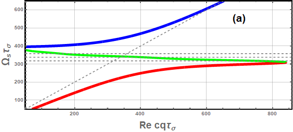
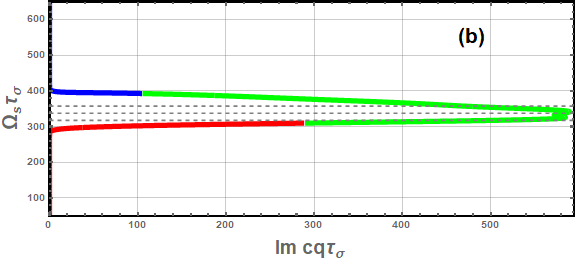
Figure 1: The polariton dispersion curves, $\Omega_{s}(\mathbf{q})$, (eq. 34) for real (a) and imaginary (b) parts of the wavevector $q$. The red/blue curves correspond to the lower/upper polariton branches, the green curve is the leaky part. The model parameters are obtained by fitting the TC dye experimental absorption spectrum in Ref.¹⁴: $K(0)\tau_{\sigma}^{2}=80$, $Q\tau_{\sigma}=84$, $\omega_{st}\tau_{\sigma}=28.6$, $\omega_{0}\tau_{\sigma}=20$, $X_{0}^{2}=0.454$, $\omega_{el}\tau_{\sigma}=303.2$, $1/\tau_{\sigma}=75\,cm^{-1}$.

In Fig.1 we plot the EP dispersion curves, Eqs.(34) and (36), with the model parameters tuned to the experimental observation of the polariton spectrum of the TC dye molecules nanofiber ¹. To satisfy Eqs.(34), the wavevector $q$ has to have a non-zero imaginary part, $q=q^{\prime}+iq^{\prime\prime}$. The imaginary part of wavevector $q^{\prime\prime}$ as a function of the polariton frequency is plotted in Fig.1 b. In the leaky part of the obtained polariton dispersion, i.e. in the range of frequencies corresponding to the gap between the lower and the upper polariton branches (green line), the value of $q^{\prime\prime}$ reaches its largest values. It can be considered as a polariton absorption spectrum.

Note that Eq.(34) can be further extended to the case of the intermolecular dipole-dipole interaction with the help of the mean-field approach^{12, 14}. The intermolecular dipole-dipole interaction, however, does not change the general behaviour of the dispersion curves. This supports the approach used in our paper.

With the help of Eqs.(33), (26), (34) and (35) we can derive the Hopfield coefficients

$$|v_{s}(\mathbf{q})|^{2}=\Bigg{[}1+\frac{\pi^{2}\Omega_{s}^{2}(\mathbf{q)}Q}{\omega_{\mathbf{q}}+\Omega_{s}(\mathbf{q})}\exp(-X_{0}^{2})\times\sum_{v}\frac{X_{0}^{2v}}{v!}\left|W_{av}^{non}[\Omega_{s}(\mathbf{q})]\right|^{2}\Bigg{]}^{-1}$$ (38)

$$\sum_{m}|\bar{u}_{smv}(\mathbf{q})|^{2}=|v_{s}(\mathbf{q})|^{2}\frac{\pi^{2}\Omega_{s}^{2}(\mathbf{q})Q}{\omega_{\mathbf{q}}+\Omega_{s}(\mathbf{q})}\\ \times\exp(-X_{0}^{2})\frac{X_{0}^{2v}}{v!}|W_{av}^{non}[\Omega_{s}(\mathbf{q})]|^{2}$$ (39)

The Hopfield coefficients calculated by Eqs.(38) and (39) are plotted for the upper (U) and the lower (L) polariton branches as a functions of the wavevector $\bm{q}$ absolute value in Fig.2.

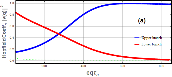
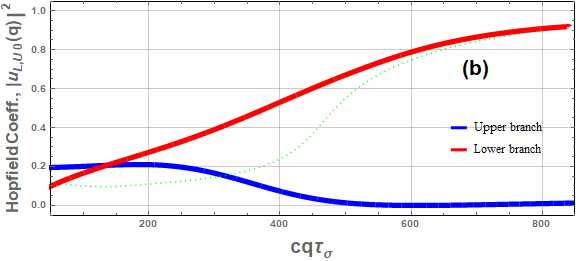
Figure 2: The Hopfield coefficients as functions of the wavevector $q=\left|\bm{q}\right|$. (a) $|v_{L}(\bm{q})|^{2}$ (red line) and $|v_{U}(\bm{q})|^{2}$ (blue line); (b) coefficients $\sum_{m}|u_{Lm0}(\bm{q})|^{2}$ (red line) and $\sum_{m}|u_{Um0}(\bm{q})|^{2}$. Other parameters are identical to those as in Fig. 1.

The obtained Hopfeld coefficients, Eqs.(38) and (39), satisfy the standard normalizing conditions.

One can see from Eq.(26) that

$$\bar{u}_{smv}(\mathbf{q})=\frac{\bar{u}_{sv}(\mathbf{q)}}{\sqrt{\mathcal{N}}}\exp(-i\mathbf{q\cdot r}_{m})$$ (40)

where

$$\bar{u}_{sv}(\mathbf{q})=-\frac{\pi g\sqrt{\mathcal{N}}}{\sqrt{\omega_{\mathbf{q}}}}e^{-X_{0}^{2}/2}\frac{X_{0}^{v}}{\sqrt{v!}}W_{av}[\Omega_{s}(\mathbf{q})]v_{s}(\mathbf{q})$$ (41)

does not depend on $m$. Using Eq.(33), we derive

$$[p_{s\mathbf{q}},p_{s\mathbf{q}}^{{\dagger}}]=|v_{s}(\mathbf{q)|}^{2}+\sum\limits_{v}|\bar{u}_{sv}(\mathbf{q)}|^{2}=1$$ (42)

with

$$|\bar{u}_{sv}(\mathbf{q)|}^{2}=\sum_{m}|\bar{u}_{smv}(\mathbf{q})|^{2}.$$ (43)

4 Polariton Luminescence Spectrum

4.1 General formulas

The frequency spectrum of a light emitting system,

$$I(\omega)=2\mathrm{Re}\int_{0}^{\infty}d\tau\langle\mathbf{E}^{(-)}(t)\mathbf{E}^{(+)}(t-\tau)\rangle e^{-i\omega\tau}$$ (44)

is generally calculated from the two-time correlation function of the quantized electric field ⁴⁷, $\mathbf{\hat{E}}(\mathbf{r},t)=\mathbf{E}^{(+)}(t)+\mathbf{E}^{(-)}(t)$, obtained by the photon leakage (see coefficient $\eta_{phot}$ below) through the mirrows of a microcavity (see Fig.3).

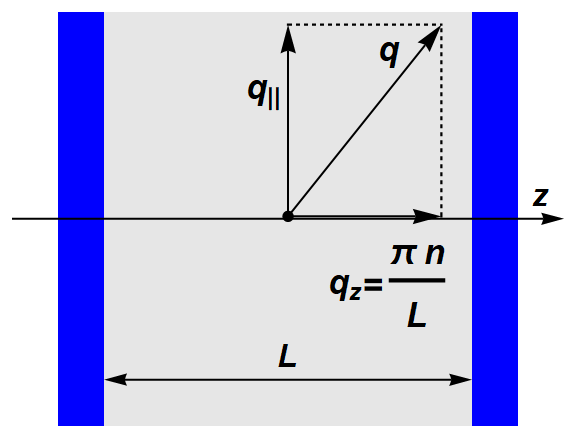
Figure 3: The molecular substance is located between the cavity mirrors separated by distance L. The in-plane wave vector $\mathbf{q}_{||}$ and its $Z$-component are shown in the figure.

The quantum averaging $\langle\dots\rangle$ indicates taking the trace over the density matrices of the phonon and polariton subsystems. Since we consider the LF vibrational system as a classical one, this procedure includes also stochastic averaging (see below). To relate this out field with intracavity one, we will use the quasimode approximation ⁴⁸, according to which the in-out coupling conserves the in-plane wave vector $\mathbf{q}_{||}$. Then one can use $\mathbf{q}_{||}$ to denote external (emitted) photons ^{49, 19, 20}, and

$$\mathbf{E}^{(+)}=[\mathbf{E}^{(-)}]^{{\dagger}}=i\sqrt{2\pi\hbar\omega_{\mathbf{q}_{||}}}\bar{a}_{\mathbf{q}_{||}}u_{\mathbf{q}_{||}}(\mathbf{r)}e^{-i\omega_{\mathbf{q}_{||}}t}$$ (45)

where $\bar{a}_{\mathbf{q}_{||}}$ is the external photon annihilation operator, the amplitude $u_{\mathbf{q}_{||}}(\mathbf{r})$ describes the field spatial dependence. Substituting Eq.(45) into Eq.(44), we obtain

$$I(\omega)=4\pi\hbar\omega_{\mathbf{q}_{||}}|u_{\mathbf{q}_{||}}(\mathbf{r)|}^{2}\times\mathrm{Re}\int_{0}^{\infty}d\tau\left\langle\bar{a}_{\mathbf{q}_{||}}^{{\dagger}}(t)\bar{a}_{\mathbf{q}_{||}}(t-\tau)\right\rangle e^{-i\omega\tau}$$ (46)

Consider the polariton luminescence in a single-mode cavity with the eigenfrequency

$$\omega_{\mathbf{q}n}=cq/n_{0}=\frac{c}{n_{0}}\sqrt{q_{||}^{2}+q_{z}^{2}}$$ (47)

where

$$\mathbf{q=(}q\mathbf{{}_{||},}q_{z}\mathbf{)}$$ (48)

is the total wave vector, $n_{0}$ is the background refraction index of the medium between the mirrors, $q_{z}=n\pi/L$ ($n=1,2,3,...$) and $q=|\mathbf{q}|$. The intracavity photon and the exciton operators can be expressed in terms of the polariton operators by means of the inverse polariton transformation ^{50, 45}

$$a_{\mathbf{q}}=\sum\limits_{s}v_{s}^{\ast}(\mathbf{q)}p_{s\mathbf{q}},b_{mv}=\sum\limits_{s\mathbf{q}}u_{smv}^{\ast}(\mathbf{q})p_{s\mathbf{q}},$$ (49)

From Eq.(46) using Eq.(49) we get

$$I_{p\mathbf{q}_{||}}(\omega)=4\pi\eta_{phot}\sum_{ss^{\prime}}\hbar\omega_{\mathbf{q}_{||}}|u_{\mathbf{q}_{||}}(\mathbf{r)|}^{2}\mathrm{Re}\int_{0}^{\infty}d\tau e^{-i\omega\tau}\left\langle v_{s}(\mathbf{q)}v_{s^{\prime}}^{\ast}(\mathbf{q)}p_{s\mathbf{q}}^{{\dagger}}(t)p_{s^{\prime}\mathbf{q}}(t-\tau)\right\rangle,$$ (50)

where both the amplitudes $v_{s}(\mathbf{q})$ and the polariton variables has to be averaged over the phonon bath.

In the article we consider strong elecron-vibrational interaction. Therefore this interaction has been taken into account in the previous section at the calculation of the amplitudes $v_{s}(\mathbf{q})$ and $u_{smv}(\mathbf{q})$ . Moreover the amplitudes were also averaged over the variables $\alpha_{m}$, which are describing the influence of the LFOA vibrations. This enabled us to reduce the obtained polariton dispersion equation to the dispersion relation known from the dielectric theory of polaritons⁴¹. The latter indicates correctness of the averaging procedure. Therefore, since the averaging of the amplitudes $v_{s}(\mathbf{q})$ and $u_{smv}(\mathbf{q})$ has been done, we can factorize the expectation value

$$\left\langle v_{s}(\mathbf{q)}v_{s^{\prime}}^{\ast}(\mathbf{q)}p_{s\mathbf{q}}^{{\dagger}}(t)p_{s^{\prime}\mathbf{q}}(t-\tau)\right\rangle=\langle v_{s}(\mathbf{q)}v_{s^{\prime}}^{\ast}(\mathbf{q)\rangle\langle}p_{s\mathbf{q}}^{{\dagger}}(t)p_{s^{\prime}\mathbf{q}}(t-\tau)\rangle,$$ (51)

Additional arguments in favour of such factorization will be given in the next section.

4.2 Calculation of the polariton two-particle expectation value

In this section we calculate the polariton two-particle expectation value, Eq.(51). The polariton operators were defined above using the thermal averaging of the LFOA vibrations with respect to the ground electronic state. Usually the polariton excitation occurs in the range of energies where the polaritons are excitons, and therefore the excitation is followed by relaxation of the vibrational subsystem in the excited electronic state. For this reason, under the averaging $\langle\mathbf{...}\rangle$ in the term $\langle p_{s\mathbf{q}}^{{\dagger}}(t)p_{s^{\prime}\mathbf{q}}(t-\tau)\rangle$ on the right-hand side of Eq.(51) we understand the trace over the phonon bath density matrix in the excited electronic state. It is worthy to note that the factorization, Eq.(51), can be justified as follows. The amplitudes $v_{s}(\mathbf{q)}$ and $\bar{u}_{smv}(\mathbf{q)}$ (or $\bar{u}_{sv}(\mathbf{q)}$) are calculated using the averaging with respect to the ground electronic state (see the section above). At the same time, $\langle p_{s\mathbf{q}}^{{\dagger}}(t)p_{s^{\prime}\mathbf{q}}(t-\tau)\rangle$ is calculated for the emission involving relaxation in the excited electronic state. Between these events a rapid dephasing occurs, in particular, due to the HFOA vibrations. Therefore, the averages of the amplitudes $v_{s}(\mathbf{q)}$, $u_{smv}(\mathbf{q)}$ ($u_{sv}(\mathbf{q)}$) and $\langle p_{s\mathbf{q}}^{{\dagger}}(t)p_{s^{\prime}\mathbf{q}}(t-\tau)\rangle$ can be carried out separately.

We rewrite the $\alpha_{m}$-dependent part of the Hamiltonian $\tilde{H}_{0}(\alpha)$, Eq.(10), the term $\tilde{H}_{0}^{\prime}(\alpha)\equiv-\hbar\sum_{m}\sum_{v=0}\alpha_{m}b_{mv}^{{\dagger}}b_{mv}$, through the polariton variables. Using Eqs.(31), (41) and (49), we write

$$\tilde{H}_{0}^{\prime}(\alpha)=-\hbar\sum\limits_{m}\sum\limits_{v=0}\alpha_{m}b_{mv}^{{\dagger}}b_{mv}=-\hbar\sum_{\mathbf{qq}^{\prime}}\alpha(\mathbf{q}-\mathbf{q}^{\prime})\sum\limits_{v=0,s,s^{\prime}}\bar{u}_{sv}(\mathbf{q})\bar{u}_{s^{\prime}v}^{\ast}(\mathbf{q}^{\prime})p_{s\mathbf{q}}^{{\dagger}}p_{s^{\prime}\mathbf{q}^{\prime}},$$ (52)

where

$$\alpha(\mathbf{q}-\mathbf{q}^{\prime})=\frac{1}{\mathcal{N}}\sum\limits_{m}\alpha_{m}\exp[-i(\mathbf{q}-\mathbf{q}^{\prime})\cdot\mathbf{\ r}_{m}].$$ (53)

The polariton operators obey the Heisenberg equations $\frac{\partial p_{s\mathbf{q}}(t)}{\partial t}=\frac{i}{\hbar}[\tilde{H}+\tilde{H}_{0}^{\prime}(\alpha),p_{s\mathbf{q}}(t)]$, which explicit form is

$$\frac{\partial p_{s\mathbf{q}}(t)}{\partial t}=-i\Omega_{s}(\mathbf{q})p_{s\mathbf{q}}(t)++i\sum\limits_{v\mathbf{q}^{\prime}s^{\prime}}\bar{u}_{sv}(\mathbf{q})\bar{u}_{s^{\prime}v}^{\ast}(\mathbf{q}^{\prime})\alpha(\mathbf{q}-\mathbf{q}^{\prime})p_{s^{\prime}\mathbf{q}^{\prime}}(t).$$ (54)

Here we have used Bose commutation relations for the polaritons.

Since other OAHF vibration states with $v\geqslant 1$ relax very fast (see discussion above), only the vibrationless state $v=0$ with respect to the HFOA vibration will contribute to the right-hand side of Eq.(54). The last term on the right-hand side of Eq.(54) describes coupling between different $\mathbf{q}$ and $s$ components of the polariton operator, resulting from the vibrational perturbation $\alpha(\mathbf{q}-\mathbf{q}^{\prime})$. This leads to both transitions between different polariton branches and moving of the corresponding wave packet along the dispersion curve. Note that presence of the HFOA vibrations generates a number of different polariton branches related to either $U$ or $L$ family (see the Supporting Information). However, for a weak electron-vibrational coupling with respect to the HFOA vibration, i.e. $X_{0m}<1$, increase of the vibronic index $v$ increases the energy of the corresponding polariton branches. In other words, the energy increase with the increase of $v$ is conserved also for the polariton branches with $X_{0m}<1$. The case $X_{0m}<1$ is realized in the majority of organic dyes.

4.3 Single mode cavity and semiclassical approximation

Usually they measure a luminescence signal at a specific angle corresponding to the specific values of $\mathbf{q}_{||}$ and $\mathbf{q}=(q_{||},q_{z})$, respectively. So, in the single-mode cavity we are interested in a specific value of $\mathbf{q}$. Assuming that $\mathbf{q}=\mathbf{q}^{\prime}$ in Eq.(54), we get

$$\frac{\partial\tilde{p}_{s\mathbf{q}}(t)}{\partial t}=i\alpha(0\mathbf{)}\sum\limits_{s^{\prime}\neq s}\bar{u}_{s0}(\mathbf{q})\bar{u}_{s^{\prime}0}^{\ast}(\mathbf{q})\tilde{p}_{s^{\prime}\mathbf{q}}e^{i(d_{s\mathbf{q}}-d_{s^{\prime}\mathbf{q}})t}$$ (55)

where we put $p_{s\mathbf{q}}(t)=\tilde{p}_{s\mathbf{q}}\exp(-id_{s\mathbf{q}}t)$ and denoted

$$d_{s\mathbf{q}}=\Omega_{s}(\mathbf{q)-}\alpha(0)|\bar{u}_{s0}(\mathbf{q})|^{2}.$$ (56)

Eq.(55) includes the last term on the right-hand side of Eq.(54) only at the largest value of the vibrational perturbation $\alpha(\mathbf{q}-\mathbf{q}^{\prime})$ for $\mathbf{q}^{\prime}=\mathbf{q}$, $\alpha(0\mathbf{)}$. The corresponding processes for $\mathbf{q}^{\prime}\neq\mathbf{q}$ describe polariton relaxation along the dispersion curve and result in the change of the population of polaritons with wave vector $\mathbf{q}$. The latter rather effects the luminescence intensity $I_{p\mathbf{q}_{||}}(\omega)$ than change its spectrum in the slow modulation limit under consideration in this section, and will be studied elsewhere.

To solve the problem, first, we use the semiclassical approximation ⁵¹ considering the quantity $\alpha_{m}$ as time-independent. Physically, the approximation is applicable for the slow modulation limit and means that only vertical (Frank-Condon) electron-vibrational transitions take place. Generalization to the case of arbitrary modulation and accounting for the non-vertical transitions will be carried out below in assumption of the Gauss-Markov process.

In the semiclassical approximation we have a couple of Eqs.(55) written for each polariton branch $s,s^{\prime}=U,L$. Solving them for a specific case of equal initial excitation of both polariton branches, with the help of Eq.(50) in the steady-state regime ($t=0$) we get

$$I_{p\mathbf{q}_{||}}(\omega)=4\pi\eta_{phot}\hbar\omega_{\mathbf{q}_{||}}|u_{\mathbf{q}_{||}}(\mathbf{r)|}^{2}\mathrm{Re}\int_{0}^{\infty}d\tau e^{-i\omega\tau}\\ \times\Bigg{\langle}e^{i\frac{d_{U\mathbf{q}}+d_{L\mathbf{q}}}{2}\tau}\sum_{s=U,L}\Big{[}\langle|v_{s}(\mathbf{q)|}^{2}\mathbf{\rangle}P_{ss}(\mathbf{q,}\tau)+\langle v_{s}(\mathbf{q)}v_{s^{\prime}}^{\ast}(\mathbf{q)\rangle}P_{ss^{\prime}}(\mathbf{q,}\tau)\Big{]}\Bigg{\rangle}$$ (57)

The diagonal element $P_{ss}(\mathbf{q,}\tau)$ is expressed by the formula

$$P_{ss}(\mathbf{q,}\tau)=\frac{|\tilde{p}_{\mathbf{q}}(0)|^{2}}{2}\sum_{+,-}\left[1\pm\frac{2\alpha(0\mathbf{)}\bar{u}_{U0}\bar{u}_{L0}+d_{s\mathbf{q}}-d_{s^{\prime}\mathbf{q}}}{\sqrt{(d_{L\mathbf{q}}-d_{U\mathbf{q}})^{2}+4\bar{c}}}\right]\times e^{\mp\frac{i\tau}{2}\sqrt{(d_{L\mathbf{q}}-d_{U\mathbf{q}})^{2}+4\bar{c}}}.$$ (58)

In both equations (eqs. 57, 58) it is assumed that $s\neq s^{\prime}$. The off-diagonal terms $P_{ss^{\prime}}(\mathbf{q,}\tau)$ are $P_{LU}(\mathbf{q,}\tau)=P_{UL}^{\ast}(\mathbf{q,}\tau)=P_{LL}(\mathbf{q,}\tau)=P_{UU}^{\ast}(\mathbf{q,}\tau)$ and $\bar{c}=\alpha^{2}(0)|\bar{u}_{U0}(\mathbf{q})\bar{u}_{L0}^{\ast}(\mathbf{q})|^{2}$. To perform the integration with respect to $\tau$ on the right-hand side of Eq.(57) we use the $\delta$-function integral representation $\mathrm{Re}\int_{0}^{\infty}d\tau e^{ix\tau}=\pi\delta(x)$.

On the next step we take averaging over the phonon bath, i.e. averaging over $\alpha_{m}$, in the resulting integral Eq.(57). Since $\alpha_{m}$ are normally distributed stochastic variables, which distribution is defined by the density matrix element corresponding to the excited electronic state

$$\rho_{22}^{(0)}(\alpha_{m})=[2\pi K(0)]^{-1/2}e^{-\frac{(\alpha_{m}-\omega_{st})^{2}}{2K(0)}},$$ (59)

their normalized sum, $\alpha(0)=\frac{1}{\mathcal{N}}\sum_{m}\alpha_{m}\equiv\frac{1}{\mathcal{N}}A$, is also a Gaussian variable. Then the probability density $\alpha(0)$ is

$$\rho_{22}\left(\alpha(0)\right)=[2\pi K(0)k_{N}]^{-1/2}e^{\frac{(\alpha(0)-\omega_{st})^{2}}{2K(0)k_{N}}}$$ (60)

where

$$k_{N}=(\mathcal{N+}2\sum_{i<j}^{\mathcal{N}}r_{ij})/\mathcal{N}^{2},$$ (61)

$0\leqslant r_{ij}\leqslant 1$ are the correlation coefficients that are different from zero when the LFOA vibrations include both the intra- and the intermolecular ones.

Assumption of the intramolecular nature of the LFOA vibrations, $\alpha_{m}$, allows us to conclude that in this case they are statistically independent, so that the coefficient $k_{N}$ is equal to $k_{N}=1/\mathcal{N}$. In another extreme case when the LFOA vibrations are intermolecular ones, correlation coefficients $r_{ij}=1$, and $k_{N}=1$.

The averaging $\langle(...)\rangle$ in Eq.(57) has to be done by using the probability density $\rho_{22}\left(\alpha(0)\right)$ and it reduces to the calculation of the integral $\langle(...)\rangle=\int_{-\infty}^{\infty}d\alpha(0)\rho_{22}\left(\alpha(0)\right)(...)$. Using Eqs.(57), (58) and (60), we get

$$I_{p\mathbf{q}_{||}}(\omega)=\frac{4\pi^{2}\eta_{phot}\hbar\omega_{\mathbf{q}_{||}}|u_{\mathbf{q}_{||}}(\mathbf{r)|}^{2}|\tilde{p}_{\mathbf{q}}(0)|^{2}}{\sqrt{2\pi k_{N}K(0)T^{2}(\omega)}}\exp\left\{-\frac{[(\omega-\Omega_{U})(\omega-\Omega_{L})+\omega_{st}T(\omega)]^{2}}{2k_{N}K(0)T^{2}(\omega)}\right\}\\ \times\frac{(\omega-\Omega_{L})\bar{u}_{U0}+(\omega-\Omega_{U})\bar{u}_{L0}}{|T(\omega)|}\sum\limits_{s=L,U}[\langle|v_{s}(\mathbf{q)|}^{2}\mathbf{\rangle+\langle}v_{s^{\prime}}\mathbf{(\mathbf{q)}}v_{s}^{\ast}\mathbf{(\mathbf{q)\rangle}]}(\omega-\Omega_{s^{\prime}})\bar{u}_{s0}$$ (62)

Here $\tilde{p}_{L\mathbf{q}}(0)=\tilde{p}_{U\mathbf{q}}(0)\equiv\tilde{p}_{\mathbf{q}}(0)$, $s\neq s^{\prime}$, $T(\omega)=(\omega-\Omega_{U})|\bar{u}_{L0}(\mathbf{q})|^{2}+(\omega-\Omega_{L})|\bar{u}_{U0}(\mathbf{q})|^{2}$ and we consider $\langle v_{s^{\prime}}(\mathbf{q})v_{s}^{\ast}(\mathbf{q)\rangle}$ as a real-valued. Note, Eq.(62) shows that the luminescence spectrum is narrowing with the intramolecular nature of the LFOA vibrations ($k_{N}=1/\mathcal{N}$) as the number of molecules increase (the term $k_{N}K(0)=K(0)/\mathcal{N}$ in the exponent), though such dependence can be compensated at weak exciton-photon coupling as the Hopfield coefficients become proportional to $Q$ and $\mathcal{N}$, i.e. $|\bar{u}_{s0}(\mathbf{q})|^{2}\sim Q\sim\mathcal{N}$ (see Eqs.(30), (39) and (43)). In contrast, for a strong exciton-photon interaction when $|\bar{u}_{s0}|^{2}$ do not depend on $\mathcal{N}$ the spectral narrowing can be observed. The latter depends also on the strength of correlations between different molecules. The effect is weakened when the LFOA vibrations include both intra- and intermolecular contributions, and disappears when the LFOA vibrations are intermolecular ones ($k_{N}=1$).

The narrowing of the polariton luminescence spectrum by increasing the number of molecules resembles the exchange (motional) narrowing in the absorption of molecular aggregates ⁵². The difference lies in the nature of the interaction responsible for the exchange effects. In molecular aggregate, this is the nearest-neighbour intermolecular coupling (Coulomb interaction), and in the case of polariton luminescence, this is a retarded interaction. Indeed, the width of a vibronic transition in a single molecule is due to the LFOA vibrations. The retarded interaction leads to the delocalization of a polariton and to averaging over the various configurations of the LFOA intramolecular vibrational subsystems. This motional narrowing effect reduces the the bandwidth of the molecular vibronic transitions. It is worthy to note that our model is more general, and unlike Ref.⁵², is not limited by static inhomogeneous broadening.

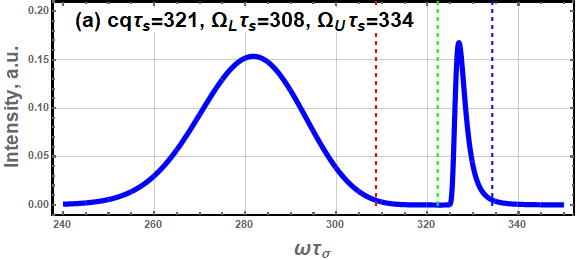
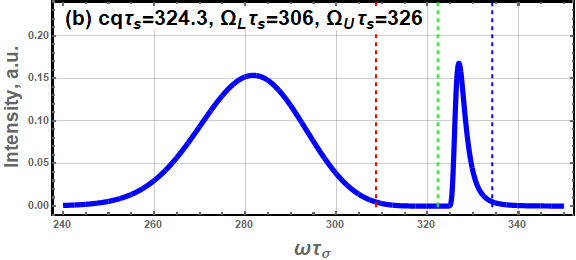
Figure 4: Luminescence spectra of molecules in a single-mode cavity in the case of the intermolecular nature of the LFOA vibrations ($k_{N}=1$) for $Q\tau_{\sigma}=2$, $K(0)\tau_{\sigma}^{2}=120$ and a) $cq\tau_{\sigma}=321$, $X_{0m}^{2}<<1$ (a single vibronic transition); b) $cq\tau_{\sigma}=324$, $X_{0m}^{2}=0.49$ (involving various vibronic transitions). The dashed lines correspond to the frequency of the lower polariton branch (red), upper polariton branch (blue) and to the ”zero” frequency (green).

Our non-Markovian theory enables us to consider both small and large splitting between the upper and the lower polariton branches compared to the spectral (homogeneous or inhomogeneous) broadening. The luminescence spectra of molecules, Eq.(62), in the case of the intermolecular nature of the LFOA vibrations, placed in a single-mode cavity at the splitting having the same order of magnitude as the inhomogeneous broadening ($K(0)\tau_{\sigma}^{2}=120$) of the molecular spectra, are presented in Fig.4. The plots in Fig.5 show behaviour of the $L$ and $U$ polariton dispersion branches (a); the Hopfield coefficients $|v_{L,U}(\mathbf{q})|^{2}$ describing the photon contributions (b); and the coefficients $|\bar{u}_{L,U0}(\mathbf{q})|^{2}$ describing the exciton contributions (c) as functions of the wave number.

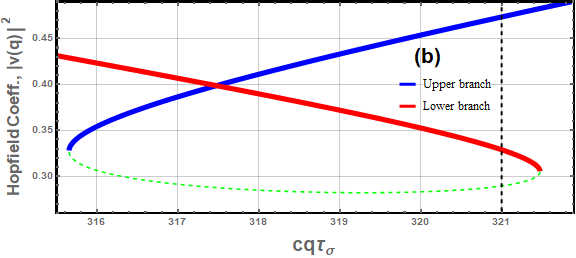
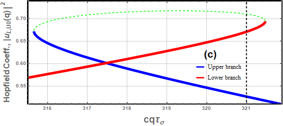
Figure 5: The EP dispersion curves (a) plotted for a single vibronic transition ($X_{0m}^{2}<<1$) at $Q\tau_{\sigma}=2$, $K(0)\tau_{\sigma}^{2}=120$; (b) The Hopfield coefficient $\left|v(\mathbf{q})\right|^{2}$ and (c) the Hopfield coefficients $\left|\bar{u}_{L0}(\mathbf{q})\right|^{2}$ and $\left|\bar{u}_{U0}(\mathbf{q})\right|^{2}$. The blue lines correspond to the upper polariton branch, and the red lines - to the lower polariton branch. The vertical black dashed line corresponds to the cavity mode wavevector chosen for the plot in Fig. 4 a.

It is believed that the polariton states are not formed, when the molecular resonances broadening is close to, or exceeds the splitting between the upper and the lower polariton branches. In contrast, for these conditions our non-Markovian theory demonstrates the main characteristic features of the Fano resonance ⁵³. Remind, that the Fano resonance is a widespread phenomenon associated with the characteristic “zero” frequency, at which the spectrum is zero, $I_{p\mathbf{q}_{||}}(\omega_{zero})=0$, and a peculiar asymmetric and ultra-sharp line shape. Such specific spectral features has found applications in a large variety of prominent optical devices ^{54, 55}. One can easily see presence of the zero frequency from Eq.(62), it becomes zero when the term $(\omega-\Omega_{L})\bar{u}_{U0}+(\omega-\Omega_{U})\bar{u}_{L0}$ in the right-hand side of Eq.(62) is zero. This gives

$$\omega_{zero}=\frac{\bar{u}_{U0}\Omega_{L}+\bar{u}_{L0}\Omega_{U}}{\bar{u}_{U0}+\bar{u}_{L0}}.$$ (63)

The “zero” frequency together with the frequencies of the lower and upper polariton branches are shown in Fig.4.

To conclude the section, we emphasize that the result Eq.(62) predicts the non-Markovian Fano resonance in the polariton luminescence, which appears because of interference of the contributions from the upper and the lower polariton branches.

4.4 Large splitting of the upper and lower polariton branches. Hot luminescence.

In the molecular systems based on the organic dyes^{1, 12} the dispersion splitting can reach the values $\sim 6000-8000$ $cm^{-1}$. At large splitting between the upper and lower polariton branches the terms with $s=s^{\prime}$ in Eqs.(50) and (51) produce the main contribution to the polariton luminescence. For large detuning $\Omega_{s}(\mathbf{q)-}\Omega_{s^{\prime}}(\mathbf{q})$ ($s\neq s^{\prime}$) the polariton operators are approximated as follows

$$p_{s\mathbf{q}}(\alpha(0),t-\tau)\approx p_{s\mathbf{q}}(\alpha(0),t)\exp(id_{s\mathbf{q}}\tau),$$ (64)

so that

$$\sum\limits_{ss^{\prime}}\langle v_{s}(\mathbf{q)}v_{s^{\prime}}^{\ast}(\mathbf{q)\rangle\langle}p_{s\mathbf{q}}^{{\dagger}}(t)p_{s^{\prime}\mathbf{q}}(t-\tau)\rangle\approx\sum\limits_{s}\langle|v_{s}(\mathbf{q)|}^{2}\mathbf{\rangle\langle}p_{s\mathbf{q}}^{{\dagger}}(t)p_{s\mathbf{q}}(t-\tau)\rangle.$$ (65)

In the slow modulation limit the average $\mathbf{\langle}p_{s\mathbf{q}}^{{\dagger}}(t)p_{s\mathbf{q}}(t-\tau)\rangle$ can be represented as
$\langle p_{s\mathbf{q}}^{{\dagger}}p_{s\mathbf{q}}(\alpha(0),t)\exp(id_{s\mathbf{q}}\tau)\rangle$, where $p_{s\mathbf{q}}^{{\dagger}}p_{s\mathbf{q}}(\alpha(0),t)=\hat{n}_{s\mathbf{q}}(\alpha(0),t)$ is the polariton population of the branch $s$, and

$$\mathrm{Re}\int_{0}^{\infty}d\tau\mathbf{\langle}p_{s\mathbf{q}}^{{\dagger}}(t)p_{s\mathbf{q}}(t-\tau)\rangle\exp(-i\omega\tau)=\pi\mathbf{\langle}p_{s\mathbf{q}}^{{\dagger}}p_{s\mathbf{q}}(\alpha(0),t)\delta(d_{s\mathbf{q}}-\omega)\rangle.$$ (66)

Since $\alpha(0)=A/\mathcal{N}$ is a stochastic Gaussian variable, one can average the product $p_{s\mathbf{q}}^{{\dagger}}(t)p_{s\mathbf{q}}(t-\tau)$ over the stochastic process using  the conditional probability density of the Gaussian process

$$P\left(\alpha(0),t;\alpha^{\prime}(0),0\right)=\frac{1}{\sqrt{2\pi\sigma\left(t\right)/\mathcal{N}}}\exp\left\{-\frac{\left[(\alpha(0)-\omega_{st})-(\alpha^{\prime}(0)-\omega_{st})S\left(t\right)\right]^{2}}{2\sigma\left(t\right)/\mathcal{N}}\right\}.$$ (67)

It is obtained from the conditional probability density distribution of $\alpha_{m}$,

$$P\left(\alpha_{m},t;\alpha_{m}^{\prime},0\right)=\frac{1}{\sqrt{2\pi\sigma\left(t\right)}}\exp\left\{-\frac{\left[(\alpha_{m}-\omega_{st})-(\alpha_{m}^{\prime}-\omega_{st})S\left(t\right)\right]^{2}}{2\sigma\left(t\right)}\right\}$$ (68)

in the case of statistically independent $\alpha_{m}$. In another extreme case when the LFOA vibrations are intermolecular ones, Eq.(68) will be also valid for $\alpha(0)$. To combine these extreme cases we write

$$P\left(\alpha(0),t;\alpha^{\prime}(0),0\right)=\frac{1}{\sqrt{2\pi\tilde{k}_{N}\sigma(t)}}\exp\left\{-\frac{\left[(\alpha(0)-\omega_{st})-(\alpha^{\prime}(0)-\omega_{st})S(t)\right]^{2}}{2\tilde{k}_{N}\sigma(t)}\right\}.$$ (69)

The parameter $\tilde{k}_{N}$ equals $1/\mathcal{N}$ for the intramolecular LFOA vibrations ($\alpha_{m}$ are statistically independent), and $\tilde{k}_{N}=1$ for the LFOA vibrations having the intermolecular nature. The variance $\sigma(t)=K(0)\left[1-S^{2}\left(t\right)\right]$, and $S(t)\equiv K(t)/K(0)$. In the long time limit, the distributions $P\left(\alpha_{m},t;\alpha_{m}^{\prime},0\right)$ and $P\left(\alpha(0),t;\alpha^{\prime}(0),0\right)$ tend to the equilibrium density matrices of LFOA vibraions in the excited state, Eqs.(59) and (60), respectively. It is worthy to note that in general $S(t)$ is not necessary an exponential function. Then the averaging in Eq.(66) is reduced to the calculation of the integral

$$\langle p_{s\mathbf{q}}^{{\dagger}}p_{s\mathbf{q}}(\alpha(0),t)\delta(d_{s\mathbf{q}}-\omega)\rangle=n_{s\mathbf{q}}(\alpha^{\prime}(0),0)\\ \times\int_{-\infty}^{\infty}d\alpha(0)P\left(\alpha(0),t;\alpha^{\prime}(0),0\right)\delta\left[\Omega_{s}(\mathbf{q})-|\bar{u}_{s0}(\mathbf{q})|^{2}\alpha(0)-\omega\right]$$ (70)

with $n_{s\mathbf{q}}(\alpha^{\prime}(0),0)=\left\langle p_{s\mathbf{q}}^{{\dagger}}p_{s\mathbf{q}}(\alpha^{\prime}(0),0)\right\rangle$. Using Eqs.(50), (51), (65), (66), (69) and (70), we get the time-dependent spectrum of the hot (non-equilibrium) luminescence

$$I_{p\mathbf{q}_{||}}(\omega,t)=4\pi^{2}\sum_{s}\eta_{phot}\hbar\omega_{\mathbf{q}_{||}}n_{s\mathbf{q}}(\alpha^{\prime}(0),0)\frac{|u_{\mathbf{q}_{||}}(\mathbf{r)|}^{2}\langle|v_{s}(\mathbf{q)|}^{2}\mathbf{\rangle}}{\sqrt{2\pi\tilde{k}_{N}\sigma\left(t\right)|\bar{u}_{s0}(\mathbf{q})|^{4}}}\\ \times\exp\Bigg{\{}-\frac{1}{2\tilde{k}_{N}\sigma\left(t\right)|\bar{u}_{s0}(\mathbf{q})|^{4}}\Big{[}(\Omega_{s}(\mathbf{q)}-\omega-\omega_{st}|\bar{u}_{s0}(\mathbf{q})|^{2})-(\alpha^{\prime}(0)-\omega_{st})|\bar{u}_{s0}(\mathbf{q})|^{2}S\left(t\right)\Big{]}^{2}\Bigg{\}}$$ (71)

Since $S(0)=1$, the spectrum is centred around the frequency $\Omega_{s}(\mathbf{q})-\alpha^{\prime}(0)$ and is very narrow for $t\rightarrow 0$, $I_{p\mathbf{q}_{||}}(\omega,0)\sim\delta[\Omega_{s}(\mathbf{q})-\alpha^{\prime}(0)-\omega]$. Remind that Eq.(71) is derived using the slow modulation limit where the time instant $t$ might be smaller than $\tau_{\sigma}$, but must be larger than the irreversible dephasing time of the vibronic transition ^{31, 32, 56, 23, 24}. The right-hand side of Eq.(71) describes the time-dependent Gaussian spectrum, which center moves from the initial frequency $\Omega_{s}(\mathbf{q})-\alpha^{\prime}(0)$ to the frequency $\Omega_{s}(\mathbf{q})-\omega_{st}|\bar{u}_{s0}(\mathbf{q})|^{2},$ and broadens over time. For long times $t>>\tau_{\sigma}$, the spectrum tends to the value

$$I_{p\mathbf{q}_{||}}(\omega,\infty)=4\pi^{2}\eta_{phot}\hbar\omega_{\mathbf{q}_{||}}|u_{\mathbf{q}_{||}}(\mathbf{r)|}^{2}\\ \times\sum_{s}\frac{\langle|v_{s}(\mathbf{q)|}^{2}\mathbf{\rangle}n_{s\mathbf{q}}(\alpha^{\prime}(0\mathbf{)},0)}{\sqrt{2\pi\tilde{k}_{N}K(0)|\bar{u}_{s0}(\mathbf{q})|^{4}}}\exp\left\{-\frac{\left[\Omega_{s}(\mathbf{q)}-\omega-\omega_{st}|\bar{u}_{s0}(\mathbf{q})|^{2}\right]^{2}}{2\tilde{k}_{N}K(0)|\bar{u}_{s0}(\mathbf{q})|^{4}}\right\}$$ (72)

with both the first, $\Omega_{s}(\mathbf{q)}-\omega_{st}|\bar{u}_{s0}(\mathbf{q})|^{2}$, and the second central moments, $\tilde{k}_{N}K(0)|\bar{u}_{s0}(\mathbf{q})|^{4}$, depending on the exciton contribution to the polariton. In other words, transition to the polariton degrees of freedom in our calculations results in replacement of the correlation function, $K(0)$, and the Stokes shift, $\omega_{st}$, generated by the LFOA vibrations, by the corresponding quantities multiplied by the factors $|\bar{u}_{s0}(\mathbf{q)}|^{4}$ and $|\bar{u}_{s0}(\mathbf{q})|^{2}$ (up to factor $\tilde{k}_{N}$), respectively. In contrast, in Ref.¹⁵, the authors were focused on the elastic cavity emission and constrained themselves to a specific case, when the polariton linewidth is the mean of the cavity and of the molecular linewidth, although this holds only when the cavity frequency is in resonance with the electron transition.

The time dependent spectrum of the light emitting polariton system, Eq.(71), is shown in Fig.6 when the lower polariton branch is initially excited. Note that since $\bar{u}_{L0}(\mathbf{q})\neq\bar{u}_{U0}(\mathbf{q})$, the hot luminescence dynamics differ quantitatively for the lower and for the upper polariton branches.

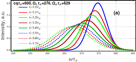
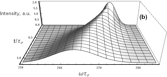
Figure 6: The time-dependent spectrum of molecules in a single-mode cavity ($cq\tau_{\sigma}=500$) in the case of the intermolecular nature of the LFOA vibrations ( $\tilde{k}_{N}=1$), Eq.( 71), plotted as a function of time $t$ and (a) frequency $\omega$, and its cross-sections (b) at different instants of time for $\alpha^{\prime}(0)=0$. The model parameters are the same as in Fig.1.

It is worthy to note that Eqs.(71) and (72) do not include further relaxation along the polariton branches to the value of $\mathbf{q}=(q_{||}=0,q_{z})$ (see the comment below Eq.(56)). This relaxation leads to a further change in luminescence intensity $I_{p\mathbf{q}_{||}}(\omega)$. The synergy of the mechanism discussed in this section and the relaxation along the polariton branches will be considered elsewhere.

4.5 Averaging with respect to the LFOA vibrations when the slow modulation limit is not implemented.

In the case of the intramolecular LFOA vibrations, i.e. when the stochastic variables $\alpha_{m}$ are statistically independent, and the value of $\tilde{k}_{N}K(0)\mathcal{=}K(0)/\mathcal{N}$ in Eqs.(71) and (72) is much smaller than $K(0)$, which is the case at large total number of molecules, $\mathcal{N}>>1$, the slow modulation limit ($\tau_{\sigma}^{2}K(0)/\mathcal{N}>>1$) cannot be taken, and the semiclassical approximation made in the section ”Single mode cavity and semiclassical approximation”, which is based on the frozen nuclear configuration assumption, ceases to be correct.

In this section we calculate the equilibrium polariton luminescence spectrum without the constrain of the slow modulation approximation. For the steady-state conditions the luminescence polariton spectrum is determined by the Fourier transform of the polariton correlation function $\mathbf{\langle}p_{s\mathbf{q}}^{{\dagger}}(\tau)p_{s\mathbf{q}}(0)\rangle$ where $p_{s\mathbf{q}}^{{\dagger}}(t)$ obeys the hermitian conjugate of Eq.(54). Setting $p_{s\mathbf{q}}^{{\dagger}}(t)=\bar{p}_{s\mathbf{q}}^{{\dagger}}\exp[i\Omega_{s}(\mathbf{q)}t]$, we obtain

$$\frac{\partial\bar{p}_{s\mathbf{q}}^{{\dagger}}}{\partial t}=-i|\bar{u}_{s0}(\mathbf{q})|^{2}\alpha(0)\bar{p}_{s\mathbf{q}}^{{\dagger}}-i\bar{u}_{s0}^{\ast}(\mathbf{q})\bar{u}_{s^{\prime}0}(\mathbf{q})\alpha(0\mathbf{)}\bar{p}_{s^{\prime}\mathbf{q}}^{{\dagger}}e^{i[\Omega_{s^{\prime}}(\mathbf{q)}-\Omega_{s}(\mathbf{q})]t},$$ (73)

where $s\neq s^{\prime}$. The expectation value of the polariton operator obeys the equation

$$\frac{\partial\langle\bar{p}_{s\mathbf{q}}^{{\dagger}}(\alpha(0),t)\rangle}{\partial t}=-i|\bar{u}_{s0}(\mathbf{q})|^{2}\alpha(0\mathbf{)}\langle\bar{p}_{s\mathbf{q}}^{{\dagger}}(\alpha(0\mathbf{),}t\mathbf{)\rangle}\\ -i\bar{u}_{s^{\prime}0}(\mathbf{q})\bar{u}_{s0}^{\ast}(\mathbf{q})\alpha(0\mathbf{)}\langle\bar{p}_{s^{\prime}\mathbf{q}}^{{\dagger}}(\alpha(0),t)e^{i[\Omega_{s}(\mathbf{q)}-\Omega_{s^{\prime}}(\mathbf{q)]}t}+\left.\frac{\partial\langle\bar{p}_{s\mathbf{q}}^{{\dagger}}(\alpha(0),t)\rangle}{\partial t}\right|_{rel}$$ (74)

where the last term on the right-hand side describes relaxation due to interaction of the polaritons with the LFOA vibrations. Using Eqs.(31) and (49), one gets for the derivative in Eq.(74)

$$\left.\frac{\partial\langle\bar{p}{\dagger}_{s\mathbf{q}}(\alpha(0\mathbf{),}t\mathbf{)\rangle}}{\partial t}\right|_{rel}=\bar{u}_{s0}^{\ast}(\mathbf{q})\left.\frac{\partial}{\partial t}\langle b_{\mathbf{q}0}^{{\dagger}}(\alpha(0),t)\rangle e^{-i\Omega_{s}(\mathbf{q)}t}\right|_{rel}.$$ (75)

To proceed we use the property of the Gauss-Markov stochastic process. The mean value of some function is known to satisfy the differential equation

$$\frac{\partial}{\partial t}\langle b_{\mathbf{q}0}^{{\dagger}}(\alpha_{m},t)\rangle|_{rel}=L_{22}(\alpha_{m})\langle b_{\mathbf{q}0}^{{\dagger}}(\alpha_{m},t)\rangle,$$ (76)

with the differential operator ¹⁴

$$L_{22}(\alpha_{m})=\tau_{\sigma}^{-1}\left[1+\frac{(\alpha_{m}-\omega_{st})\partial}{\partial(\alpha_{m}-\omega_{st})}+\frac{K(0)\partial^{2}}{\partial(\alpha_{m}-\omega_{st})^{2}}\right].$$ (77)

Bearing in mind Eqs.(76) and (77) we rewrite the right-hand side of Eq.(74) as

$$\bar{u}_{s0}^{\ast}(\mathbf{q})\left.\frac{\partial}{\partial t}\langle b_{\mathbf{q}0}^{{\dagger}}(\alpha(0),t)\rangle e^{-i\Omega_{s}(\mathbf{q)}t]}\right|_{rel}\\ =L_{22}\Big{[}\bar{u}_{s0}^{\ast}(\mathbf{q)}u_{s^{\prime}0}(\mathbf{q})e^{i(\Omega_{s^{\prime}}(\mathbf{q})-\Omega_{s}(\mathbf{q}))t}\langle\bar{p}_{s^{\prime}\mathbf{q}}^{{\dagger}}(\alpha(0\mathbf{),}t)\rangle+|\bar{u}_{s0}(\mathbf{q})|^{2}\langle\bar{p}_{s\mathbf{q}}^{{\dagger}}(\alpha(0),t)\rangle\Big{]}$$ (78)

where the operator $L_{22}(\alpha_{m})$ is now simplified to

$$L_{22}\equiv\tau_{\sigma}^{-1}\left[1+\alpha_{2}\frac{\partial}{\partial\alpha_{2}}+\tilde{k}_{N}K(0)\frac{\partial^{2}}{\partial\alpha_{2}^{2}}\right]$$ (79)

with $\alpha_{2}=\alpha(0)-\omega_{st}$. Here we have used the same arguments which led us to Eq.(60). After the above simplifications we formulate the set of equation for the functions

$$A(\alpha_{2},t) = \exp(-i\Lambda t/2)\langle\bar{p}_{U\mathbf{q}}^{{\dagger}}(\alpha_{2},t)\rangle+\frac{\bar{u}_{L0}}{\bar{u}_{U0}}\exp(i\Lambda t/2\mathbf{)}\langle\bar{p}_{L\mathbf{q}}^{{\dagger}}(\alpha_{2},t)\rangle$$ (80)

$$B(\alpha_{2},t) = \exp(-i\Lambda t/2)\langle\bar{p}_{U\mathbf{q}}^{{\dagger}}(\alpha_{2},t)-\frac{\bar{u}_{L0}}{\bar{u}_{U0}}\exp(i\Lambda t/2)\langle\bar{p}_{L\mathbf{q}}^{{\dagger}}(\alpha_{2},t)\rangle,$$ (81)

where $\Lambda=\Omega_{L}(\mathbf{q})-\Omega_{U}(\mathbf{q})$. The functions $A(\alpha_{2},t)$ and $B(\alpha_{2},t)$ satisfy the set of partial-derivative equations

$$\frac{\partial}{\partial t}A(\alpha_{2},t) = (|\bar{u}_{U0}|^{2}+|\bar{u}_{L0}|^{2})[-i\alpha_{2}-i\omega_{st}+L_{22}]A(\alpha_{2},t)-i\frac{\Lambda}{2}B(\alpha_{2},t)+A(\alpha_{2},0)\delta(t)$$ (82)

$$\frac{\partial}{\partial t}B(\alpha_{2},t) = (|\bar{u}_{U0}|^{2}-|\bar{u}_{L0}|^{2})(-i\alpha_{2}-i\omega_{st}\mathbf{+}L_{22})A(\alpha_{2},t)-i\frac{\Lambda}{2}A(\alpha_{2},t)+B(\alpha_{2},0)\delta(t).$$ (83)

To simplify solution of the equations we also took into account the initial conditions $A(\alpha_{2},0)$ and $B(\alpha_{2},0)$ by introducing the terms with the delta-function $\delta(t)$. The inverse transformation from the functions $A(\alpha_{2},t)$ and $B(\alpha_{2},t)$ to the functions $\langle\bar{p}_{s\mathbf{q}}^{{\dagger}}(\alpha_{2},t)\rangle$ has the form

$$\langle\bar{p}_{U\mathbf{q}}^{{\dagger}}(\alpha_{2},t)\rangle=\frac{1}{2}e^{i\Lambda t/2}[A(\alpha_{2},t)+B(\alpha_{2},t)],$$ (84)

$$\langle\bar{p}_{L\mathbf{q}}^{{\dagger}}(\alpha_{2},t)\rangle=\frac{1}{2}\frac{\bar{u}_{U0}}{\bar{u}_{L0}}e^{-i\Lambda t/2}[A(\alpha_{2},t)-B(\alpha_{2},t)].$$ (85)

Eqs.(82) and (83) are solved in the Supporting Information.

4.5.1 Luminescence spectrum calculation

The equilibrium luminescence spectrum ($t=0$) in a single-mode cavity according to Eqs.(50) and (51) is written as

$$I_{p\mathbf{q}_{||}}(\omega)=4\pi\eta_{phot}\hbar\omega_{\mathbf{q}_{||}}|u_{\mathbf{q}_{||}}(\mathbf{r)|}^{2}\sum_{ss^{\prime}}\langle v_{s}(\mathbf{q)}v_{s^{\prime}}^{\ast}(\mathbf{q})\rangle\\ \times\langle p_{s^{\prime}\mathbf{q}}(0)\rangle\mathrm{Re}\int_{0}^{\infty}d\tau\mathbf{\langle}\bar{p}_{s\mathbf{q}}^{\prime}{\dagger}(\tau)\rangle e^{-i(\omega-\Omega_{s}(\mathbf{q}))\tau}$$ (86)

where the polariton operator $\mathbf{\langle}\bar{p}_{s\mathbf{q}}^{\prime}{\dagger}(\tau)\rangle$ includes averaging over the stochastic process described by the variable $\alpha_{2}$,

$$\langle\bar{p}_{s\mathbf{q}}^{\prime}{\dagger}(\tau)\rangle=\int d\alpha_{2}\langle\bar{p}_{s\mathbf{q}}^{{\dagger}}(\alpha_{2},\tau)\rangle$$ (87)

The latter expression means that the function $\langle\bar{p}_{s\mathbf{q}}^{\prime}{\dagger}(\tau)\rangle$ is the Fourier transform of the polariton operator $\langle\bar{p}_{s\mathbf{q}}^{{\dagger}}(\alpha_{2},\tau)\rangle$ over $\alpha_{2}$, which has to be taken at zero Fourier-conjugate variable $\varkappa$ (see the Supporting Information). At the same time $\mathbf{\langle}\bar{p}_{s\mathbf{q}}^{\prime}{\dagger}(\tau)\rangle$ can be written as the Fourier-transform of $\langle\bar{P}_{s\mathbf{q}}^{\prime}{\dagger}(\tilde{\omega}\mathbf{)\rangle}$

$$\mathbf{\langle}\bar{p}_{s\mathbf{q}}^{\prime}{\dagger}(\tau)\rangle=\frac{1}{2\pi}\int_{-\infty}^{\infty}d\tilde{\omega}\exp(i\tilde{\omega}\tau)\langle\bar{P}_{s\mathbf{q}}^{\prime}{\dagger}(\tilde{\omega}\mathbf{)\rangle}$$ (88)

where $\langle\bar{P}_{s\mathbf{q}}^{\prime}{\dagger}(0\mathbf{,}\tilde{\omega}\mathbf{)\rangle=}\int_{-\infty}^{\infty}d\tau\mathbf{\langle}\bar{p}_{s\mathbf{q}}^{\prime}{\dagger}(\tau)\rangle\exp(-i\tilde{\omega}\tau)$. Using Eq.(88), the real part of the integral on the right-hand side of Eq.(86), can be written as

$$\mathrm{Re}\int_{0}^{\infty}d\tau\mathbf{\langle}\bar{p}_{s\mathbf{q}}^{\prime}{\dagger}(\tau)\rangle\exp(-i\tilde{\omega}\tau)=-\mathrm{Im}\frac{1}{2\pi}P\int_{-\infty}^{\infty}d\tilde{\omega}^{\prime}\frac{\mathbf{\langle}\bar{P}_{s\mathbf{q}}^{\prime}{\dagger}(0,\tilde{\omega}^{\prime})\rangle}{\tilde{\omega}^{\prime}-\tilde{\omega}}+\frac{1}{2}\mathrm{Re}\langle\bar{P}_{s\mathbf{q}}^{\prime}{\dagger}(0,\tilde{\omega})\rangle,$$ (89)

where $\tilde{\omega}=\omega-\Omega_{s}(\mathbf{q)}$. The direct calculation of the first term on the right-hand side of Eq.(89) is difficult. However, this term can be expressed in terms of $\mathrm{Re}\mathbf{\langle}\bar{P}_{s\mathbf{q}}^{\prime}{\dagger}(0,\tilde{\omega})\rangle$, using  the Kramers-Kronig relations ^{57, 30, 58} (see the Supporting Information)

$$-\frac{1}{\pi}P\int_{-\infty}^{\infty}d\tilde{\omega}^{\prime}\frac{\mathrm{Im}\mathbf{\langle}\bar{P}_{s\mathbf{q}}^{\prime{\dagger}}(0,\tilde{\omega}^{\prime})\rangle}{\tilde{\omega}^{\prime}-\omega}=\mathrm{Re}\mathbf{\langle}\bar{P}_{s\mathbf{q}}^{\prime{\dagger}}(0,\tilde{\omega})\rangle$$ (90)

Then only the real part of the Fourier transform defines the luminescence spectrum

$$\mathrm{Re}\langle\bar{P}_{s\mathbf{q}}^{\prime{\dagger}}(\tilde{\omega})\rangle=\mathrm{Re}\int_{0}^{\infty}d\tau e^{-i\tilde{\omega}\tau}\langle\bar{p}_{s\mathbf{q}}^{\prime}{\dagger}(\tau)\rangle$$ (91)

According to Eqs.(84) and (85) the function $\langle\bar{P}_{s\mathbf{q}}^{\prime{\dagger}}(\tilde{\omega})\rangle$ is a linear combination of the functions $g(0,\tilde{\omega})$ and $G(0,\tilde{\omega})$, Eqs.(119), (120) and (117) of the Supporting Information, with the frequencies shifted by the factor $\Lambda/2$,

$$\langle\bar{P}_{L,U\mathbf{q}}^{{\dagger}}(\tilde{\omega})\rangle=\frac{1}{2}\left(\begin{array}[]{c}\bar{u}_{U0}/\bar{u}_{L0}\\ 1\end{array}\right)\left[G(0,\tilde{\omega}\pm\frac{\Lambda}{2})\mp g(0,\tilde{\omega}\pm\frac{\Lambda}{2})\right]$$ (92)

Using Eqs.(117), (120) of the Supporting Information and (92), we obtain

$$\mathrm{Re}\langle\bar{P}_{s\mathbf{q}}^{\prime{\dagger}}(\omega-\Omega_{s})\rangle=\langle p_{s\mathbf{q}}{\dagger}(0\mathbf{)\rangle}\\ \times\frac{\bar{u}_{L0}(\omega-\Omega_{s^{\prime}})}{T^{2}(\omega)}[\bar{u}_{U0}(\omega-\Omega_{L})+\bar{u}_{L0}(\omega-\Omega_{U})]\mathrm{Re}\frac{\Phi(1,1+\bar{x}_{f};\tilde{k}_{N}K(0)\tau_{\sigma}^{2})}{\tau_{\sigma}^{-1}\bar{x}_{f}}$$ (93)

where $s,s^{\prime}=L,U$; $s\neq s^{\prime}$, and

$$\bar{x}_{f}=\tilde{k}_{N}K(0)\tau_{\sigma}^{2}+i\tau_{\sigma}\left[\frac{(\omega-\Omega_{L})(\omega-\Omega_{U})}{T(\omega)}+\omega_{st}\right]$$ (94)

Substituting Eqs.(91) and (93) into Eq.(86), we finally get

$$I_{p\mathbf{q}_{||}}(\omega)=4\pi\eta_{phot}\hbar\omega_{\mathbf{q}_{||}}|u_{\mathbf{q}_{||}}(\mathbf{r)|}^{2}\frac{\bar{u}_{U0}(\omega-\Omega_{L})+\bar{u}_{L0}(\omega-\Omega_{U})}{T^{2}(\omega)}\mathrm{Re}\frac{\Phi(1,1+\bar{x}_{f};\tilde{k}_{N}K(0)\tau_{\sigma}^{2})}{\tau_{\sigma}^{-1}\bar{x}_{f}}\\ \times\sum_{s=L,U}|\langle p_{s\mathbf{q}}(0)\rangle|^{2}\bar{u}_{s0}(\omega-\Omega_{s^{\prime}})\left[\langle|v_{s}(\mathbf{q})|^{2}\rangle+\langle v_{s}(\mathbf{q})v_{s^{\prime}}^{\ast}(\mathbf{q})\rangle\right],$$ (95)

where $s\neq s^{\prime}$ and the equally distributed initial population is assumed, $\tilde{p}_{L\mathbf{q}}(0)=\tilde{p}_{U\mathbf{q}}(0)=\tilde{p}_{s\mathbf{q}}(0)$.

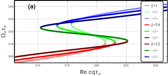
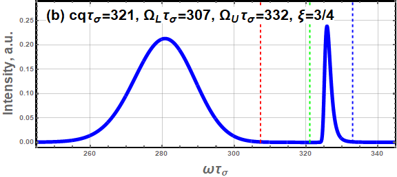
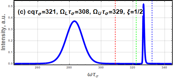
Figure 7: The dispersion curves (a) and the polariton luminescence spectrum (b, c) of molecules in a single-mode cavity in the case of the intermolecular nature of the LFOA vibrations ($\tilde{k}_{N}=1$) calculated by Eq. (95) for a single vibronic transition ($X_{0m}^{2}\ll 1$) for various $Q\tau_{\sigma}=2\xi$ and $K(0)\tau_{\sigma}^{2}=120\xi^{2}$, namely in plot (b) $Q\tau_{\sigma}=1.5$, $K(0)\tau_{\sigma}^{2}=67.5$ and (c) $Q\tau_{\sigma}=1$ and $K(0)\tau_{\sigma}^{2}=30$ (compare with Fig.4 a, where $K(0)\tau_{\sigma}^{2}=120$ and $Q\tau_{\sigma}=2$).

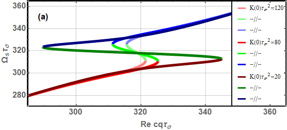
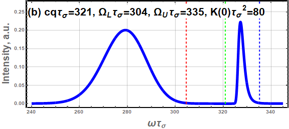
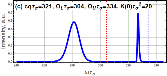
Figure 8: The dispersion curves (a) and the polariton luminescence spectrum (b, c) of molecules in a single-mode cavity in the case of the intermolecular nature of the LFOA vibrations ($\tilde{k}_{N}=1$) calculated by Eq. (95) for a single vibronic transition ($X_{0m}^{2}\ll 1$) for various $K(0)\tau_{\sigma}^{2}=80$ (b) and $20$ (c) at $Q\tau_{\sigma}=2$ (compare with Fig.4 a, where $K(0)\tau_{\sigma}^{2}=120$ and $Q\tau_{\sigma}=2$).

In the slow modulation limit when $\tau_{\sigma}^{2}\tilde{k}_{N}K(0)\mathcal{>>}1$, Eq.(95) transforms into Eq.(62). It is worthy to note that the same factor $(\omega-\Omega_{L})\bar{u}_{U0}+(\omega-\Omega_{U})\bar{u}_{L0}$ is present in both equations which determines the ”zero” frequency, Eq.(63). By this means, the luminescence spectra described by Eqs.(62) and (95) have the main characteristic features of the Fano resonances. Therefore, these equations can be viewed as a generalization of Fano resonances to the non-Markovian case. Our numerical results (Fig. 7, 8) show that the best condition for observing the Fano resonances in polariton luminescence is the limit of slow modulation, which corresponds to the inhomogeneous broadening of the molecular spectra, i.e. the extreme non-Markovian limit. The condition of the interference between the fluorescent peaks requires also that the splitting between the upper and the lower polariton branches has to be of the same order as the inhomogeneous broadening.

5 Conclusion

In our work a theory of equilibrium and non-equilibrium (hot) polariton luminescence spectra in the polariton basis was developed using the non-Markovian theory for the description of the polariton interaction with molecular vibrations. We adopted here a realistic model, according to which each member of the HFOA vibronic progression in the absorption and luminescence molecular spectra is broadened due to the presence of the LFOA vibrations $\{\omega_{\sigma}\}$. At the calculation of the polariton frequencies and the Hopfield coefficients, we average them over $\alpha_{m}$, the electron-vibration coupling related to the LFOA molecular vibrations. This enabled us to get the dispersion equation that coincides with the equation for the transverse eigenmodes of the medium.

In spite of averaging of the Hopfield coefficients over the electron-vibration coupling related to the LFOA molecular vibrations, our theory demonstrates vibrational relaxation of polaritons after excitation, since equilibrium positions of molecular vibrations in the ground and excited states do not coincide (the polaron effect). We have shown that the frequency shift and the broadening of polariton luminescence spectra strongly depend on the exciton contribution to the polariton, which itself is a function of frequency.

Our theory predicts the non-Markovian Fano resonance in the polariton luminescence due to the interference contributions from the upper and lower polariton branches, and motional narrowing of the EP luminescence spectrum in the case of the intramolecular nature of the LFOA vibrations with an increase of the number of molecules in a single-mode microcavity. In addition, the theory enables us to consider a non-equilibrium (hot) EP luminescence and opens a way for its observation in organic-based nanodevices in analogy with the hot luminescence of molecules and crystals ^{25, 26}.

The last term on the right-hand side of Eq.(54) describes EP relaxation along the polariton branches when $\mathbf{q}^{\prime}\neq\mathbf{q}$. It will be took into account elsewhere to extend our theory to the multimode cavities, wave guides, and to consider the synergy of the EP relaxation over wave numbers with the mechanism of the hot EP luminescence discussed in this paper.

The work was supported by the Ministry of Science & Technology of Israel (Grant No. 79518) and the Grant RA1900000633 for cooperation between Ariel University and Holon Institute of Technology.

Appendix A Supporting Information

A.1 Calculations of the polariton dispersion and the Hopfield coefficients

The transformation coefficients $u_{smv}$ and $v_{s}(\mathbf{q)}$ in Eq.(16) of the main text and the polariton spectrum $\Omega_{s}$ can be found by evaluating the commutator $[p_{s},\tilde{H}]/\hbar$. Using Eq.(18) and Eq.(16) together with the total Hamiltonian (15) we obtain

$$\Omega_{s}p_{s}=\Omega_{s}\left[\sum_{\mathbf{q}}v_{s}(\mathbf{q)}a_{\mathbf{q}}+\sum\limits_{mv}u_{smv}b_{mv}\right]\\ =\sum_{\mathbf{q}}\left[\omega_{\mathbf{q}}v_{s}(\mathbf{q)}+\frac{ig}{\sqrt{\omega_{\mathbf{q}}}}\sum\limits_{mv}\frac{X_{0m}^{v}}{\sqrt{v!}}e^{-\frac{X_{0m}^{2}}{2}+i\mathbf{q\cdot r}_{m}}u_{smv}(\mathbf{q})\right]a_{\mathbf{q}}\\ +\sum\limits_{mv}\left[u_{smv}(\omega_{2v}+\frac{\omega_{st}}{2}-\alpha_{m})-i\frac{X_{0m}^{v}}{\sqrt{v!}}\sum_{\mathbf{q}}\frac{g}{\sqrt{\omega_{\mathbf{q}}}}e^{-\frac{X_{0m}^{2}}{2}-i\mathbf{q\cdot r}_{m}}v_{s}(\mathbf{q)}\right]b_{mv}$$ (96)

Comparing the coefficients of $a_{\mathbf{q}}$ and $b_{mv}$, we find

$$(\Omega_{s}-\omega_{\mathbf{q}})v_{s}(\mathbf{q})=\frac{ig}{\sqrt{\omega_{\mathbf{q}}}}\sum\limits_{mv}e^{-\frac{X_{0m}^{2}}{2}+i\mathbf{q\cdot r}_{m}}\frac{X_{0m}^{v}}{\sqrt{v!}}u_{smv}$$ (97)

and

$$u_{smv}=\frac{-i}{\Omega_{s}\mathbf{-(}\omega_{2v}+\omega_{st}/2)+\alpha_{m}}\sum_{\mathbf{q}}\frac{g}{\sqrt{\omega_{\mathbf{q}}}}v_{s}(\mathbf{q)}e^{-\frac{X_{0m}^{2}}{2}-i\mathbf{q\cdot r}_{m}}\frac{X_{0m}^{v}}{\sqrt{v!}}$$ (98)

Introducing a small decay, the term $1/[\Omega_{s}-(\omega_{2v}+\omega_{st}/2)+\alpha_{m}]$ on the right-hand side of Eq.(98) can be written as

$$\lim_{\gamma\rightarrow 0}\frac{1}{\Omega_{s}-(\omega_{2v}+\omega_{st}/2)+\alpha_{m}+i\gamma}=\zeta[\Omega_{s}\mathbf{-(}\omega_{2v}+\omega_{st}/2)+\alpha_{m}]$$ (99)

where $\zeta[\omega]=\frac{P}{\omega}-i\pi\delta[\omega]$, and $P$ stands for the principal value. Substituting Eq.(99) into Eq.(98), we get Eq.(19) of the main text.

A.2 The whys and wherefores of taking LFOA vibrations into account on calculations of the polariton dispersion and the Hopfield coefficients.

It is worthy to note that in the absense of the LFOA vibrations, the number of different polariton branches $s$ is not limited by $s=U,L$. In presence of the HFOA vibrations, instead of two polariton branches one can define a family of dispersion curves related either to the upper, $U$, or the lower, $L$, families. Moreover, the $L$ family branches can cross each other at $X_{0}>1$ (see the figure below). The reason of this intersection can be explained as follows. At $X_{0}>1$, the vibronic transition $0\rightarrow 1$ and possibly the transition $0\rightarrow 2$ become stronger (the corresponding absorption intensity peaks increase) than the vibronic transition $0\rightarrow 0$. In this case, the avoided crossing gap of the $L$ and $U$ branches corresponding to the transition $0\rightarrow 0$ is smaller than that for the transitions $0\rightarrow 1$ and $0\rightarrow 2$. This eventually results in the light-induced intersection of different branches in the family of lower branches. This means that some of the polariton frequencies $\Omega_{s}(\mathbf{q})$ can be very close to each other.

For the HFOA vibration mode the cases $X_{0}<1$ and $X_{0}>1$ correspond to the limits of weak and strong electron-vibrational coupling, respectively. Therefore, the approaches based solely on the calculations of the electron system can be inappropriate for $X_{0}>1$ (see figure below). The lower family dispersion curves crossings at $X_{0}>1$ lead to the light-induced conical intersection in the polariton energy manifold, and the topological effects become important. However, the broadening caused by the presence of the LFOA vibrations, in our approach, effectively merges the different branches of the lower dispersion curves family and thus pushes the problem aside.

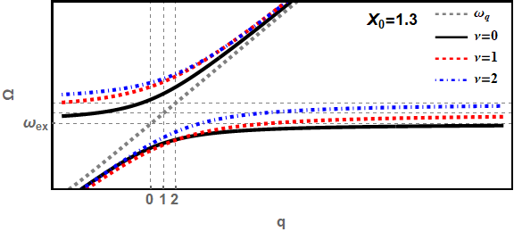
Figure 9: *

The upper and lower families of the polariton dispersion curves calculated for various vibronic levels at $X_{0}=1.3$.

A.3 Solution of Eqs.(74) of the main text for large detuning $\Omega_{U}(\mathbf{q})-\Omega_{L}(\mathbf{q}).$

Introducing the Fourier-transform

$$\Psi_{s}(\varkappa,t) = \int_{-\infty}^{\infty}d\alpha_{2}\exp(-i\varkappa\alpha_{2})\langle\bar{p}_{s\mathbf{q}}^{\prime}{\dagger}(\alpha_{2},t\mathbf{)\rangle},$$ (100)

$$\langle\bar{p}_{s\mathbf{q}}^{\prime}{\dagger}(\alpha_{2},t\mathbf{)\rangle} = \frac{1}{2\pi}\int_{-\infty}^{\infty}\Psi_{s}(\varkappa,t)\exp(i\varkappa\alpha_{2})d\varkappa$$

and applying it to Eqs.(74) of the main text, bearing in mind Eqs.(75) and (78) we get

$$\frac{\partial\Psi_{s}(\varkappa,t)}{\partial t}=\left[-i\omega_{st}+(1-\tau_{\sigma}^{-1}\varkappa)\frac{\partial}{\partial\varkappa}-\tau_{\sigma}^{-1}\tilde{k}_{N}K(0)\varkappa^{2}\right]\\ \times\left\{|\bar{u}_{s0}(\mathbf{q})|^{2}\Psi_{s}(\varkappa,t)+\bar{u}_{s0}^{\ast}(\mathbf{q)}u_{s^{\prime}0}(\mathbf{q})\Psi_{s^{\prime}}(\varkappa,t)e^{-i\big{(}\Omega_{s}(\mathbf{q})-\Omega_{s^{\prime}}(\mathbf{q})\big{)}t}\right\}.$$ (101)

Here $s\neq s^{\prime}$. For large detunings $\Omega_{s}(\mathbf{q})-\Omega_{s^{\prime}}(\mathbf{q})$ the last term on the right-hand side of Eq.(101) gives small contribution due to fast oscillations and can be neglected. Setting

$$\Psi_{s}(\varkappa,t)=\tilde{\Psi}_{s}(\varkappa,t)e^{-i|\bar{u}_{s0}(\mathbf{q})|^{2}\omega_{st}t}$$ (102)

the Eq.(101) for large detuning becomes

$$\frac{\partial\bar{\Psi}_{s}(\varkappa,\tilde{t})}{\partial\tilde{t}}\approx-\left[(-1\mathbf{+}\tau_{\sigma}^{-1}\varkappa)\frac{\partial}{\partial\varkappa}+\tau_{\sigma}^{-1}K^{\prime}(0)\varkappa^{2}\right]\bar{\Psi}_{s}(\varkappa,\tilde{t}),$$ (103)

which is the one-dimensional version of the equation obtained in Ref.⁵⁹. Here $K^{\prime}(0)=\tilde{k}_{N}K(0)$, $\tilde{t}=|\bar{u}_{s0}(\mathbf{q})|^{2}t$ and $\bar{\Psi}_{s}(\varkappa,\tilde{t})=\tilde{\Psi}_{s}(\varkappa,t).$ Returning back to the function $\tilde{\Psi}_{s}(\varkappa,t)$, we rewrite the solution of Eq.(103) as

$$\tilde{\Psi}_{s}(\varkappa,t)=B\exp\Bigg{\{}-\frac{\tilde{k}_{N}K(0)}{2}\Big{[}\varkappa^{2}+2\varkappa\tau_{\sigma}\left(1-e^{-|\bar{u}_{s0}(\mathbf{q})|^{2}t/\tau_{\sigma}}\right)\\ +2\tau_{\sigma}^{2}\left(|\bar{u}_{s0}(\mathbf{q})|^{2}t/\tau_{\sigma}-1+e^{-|\bar{u}_{s0}(\mathbf{q})|^{2}t/\tau_{\sigma}}\right)\Big{]}\Bigg{\}}$$ (104)

with $\tilde{\Psi}_{s}(0,t)=B\tilde{\Psi}_{s}^{\prime}(0,t)$, where

$$\tilde{\Psi}_{s}^{\prime}(0,t)=\exp\left\{-\tilde{k}_{N}K(0)\tau_{\sigma}^{2}\left[|\bar{u}_{s0}(\mathbf{q})|^{2}t/\tau_{\sigma}-1+e^{-|\bar{u}_{s0}(\mathbf{q})|^{2}t/\tau_{\sigma}}\right]\right\}$$ (105)

and $B=\langle p_{s\mathbf{q}}{\dagger}(0\mathbf{)\rangle}$ is a constant. Then the luminescence spectrum given by Eq.(50) of the main text can be written for the large detuning as

$$I_{p\mathbf{q}_{||}}(\omega)=4\pi\eta_{phot}\hbar\omega_{\mathbf{q}_{||}}|u_{\mathbf{q}_{||}}(\mathbf{r)|}^{2}\sum_{s}\langle|v_{s}(\mathbf{q)|}^{2}\rangle\langle|p_{s\mathbf{q}}(0)|^{2}\mathbf{\rangle}\\ \times\mathrm{Re}\int_{0}^{\infty}d\tau\tilde{\Psi}_{s}^{\prime}(0,\tau)\exp[i(\Omega_{s}(\mathbf{q)}-|\bar{u}_{s0}(\mathbf{q})|^{2}\omega_{st}-\omega)\tau]$$ (106)

where $\tilde{\Psi}_{s}^{\prime}(0,\tau)$ is the characteristic function. Calculating the integral on the right-hand side of Eq.(106), we finally obtain

$$I_{p\mathbf{q}_{||}}(\omega)=4\pi\eta_{phot}\sum_{s}\hbar\omega_{\mathbf{q}_{||}}|u_{\mathbf{q}_{||}}(\mathbf{r)|}^{2}\langle|v_{s}(\mathbf{q)|}^{2}\rangle\langle|p_{s\mathbf{q}}(0\mathbf{)|}^{2}\mathbf{\rangle}\mathrm{Re}\left[\frac{\tau_{\sigma}}{|\bar{u}_{s0}(\mathbf{q})|^{2}x_{f}}\Phi(1,1+x_{f};\tilde{k}_{N}K(0)\tau_{\sigma}^{2})\right]$$ (107)

with

$$x_{f}=\tilde{k}_{N}K(0)\tau_{\sigma}^{2}+i\tau_{\sigma}\left[\frac{\omega-\Omega_{s}(\mathbf{q)}}{|\bar{u}_{s0}(\mathbf{q})|^{2}}+\omega_{st}\right]$$ (108)

and the confluent hypergeometric function $\Phi(1,1+x_{f};\tilde{k}_{N}K(0)\tau_{\sigma}^{2})$.

In the slow modulation limit, $\tilde{k}_{N}K(0)\tau_{\sigma}^{2}>>1$, the function $\tilde{\Psi}_{s}^{\prime}(0,\tau)$ on the right-hand side of Eq. (106) becomes $\tilde{\Psi}_{s}^{\prime}(0,\tau)\simeq\exp[-\frac{\tilde{k}_{N}K(0)|\bar{u}_{s0}(\mathbf{q})|^{4}}{2}\tau^{2}]$. This leads to the polariton luminescence spectrum given by Eq. (72) of the main text, where $n_{s\mathbf{q}}(\alpha^{\prime}(0),0)=\langle|p_{s\mathbf{q}}(0)|^{2}\rangle$, and the bandwidth of which is $\sim\sqrt{\tilde{k}_{N}K(0)|\bar{u}_{s0}(\mathbf{q})|^{4}}$. For the fast modulation case, $\tilde{k}_{N}K(0)\tau_{\sigma}^{2}<<1$, and $\tau$ is large, the function $\tilde{\Psi}_{s}^{\prime}(0,\tau)$ behaves like $\tilde{\Psi}_{s}^{\prime}(0,\tau)\simeq\exp[-\Gamma|\bar{u}_{s0}(\mathbf{q})|^{2}\tau]$, where $\Gamma=\tilde{k}_{N}K(0)\tau_{\sigma}$. This results in the Lorentzian-shape spectrum

$$I_{p\mathbf{q}_{||}}(\omega)=4\pi\eta_{phot}\hbar\omega_{\mathbf{q}_{||}}|u_{\mathbf{q}_{||}}(\mathbf{r)|}^{2}\sum_{s}\frac{\Gamma\langle|v_{s}(\mathbf{q)|}^{2}\rangle\langle|p_{s\mathbf{q}}(0)|^{2}\rangle|\bar{u}_{s0}(\mathbf{q})|^{2}}{\Gamma^{2}|\bar{u}_{s0}(\mathbf{q})|^{4}+(\Omega_{s}(\mathbf{q)}-|\bar{u}_{s0}(\mathbf{q})|^{2}\omega_{st}-\omega)^{2}}.$$ (109)

One can see that in both limiting cases of the slow and the fast modulation, the bandwidth of the polariton luminescence spectrum is proportional to the square of the Hopfield coefficient corresponding to the exciton contribution to the polariton, $|\bar{u}_{s0}(\mathbf{q})|^{2}$.

A.4 Solution of Eqs.(82) and (83) of the main text

Eqs.(82) and (83) of the main text can be reduced to the second order equation for $A(\alpha_{2},t)$

$$\left[\frac{\partial^{2}}{\partial t^{2}}+\frac{\Lambda^{2}}{4}-(-i\alpha_{2}-i\omega_{st}+L_{22})\left[\left(|\bar{u}_{U0}|^{2}+|\bar{u}_{L0}|^{2}\right)\frac{\partial}{\partial t}-i\left(|\bar{u}_{U0}|^{2}-|\bar{u}_{L0}|^{2}\right)\frac{\Lambda}{2}\right]\right]A(\alpha_{2},t)\\ =-i\frac{\Lambda}{2}B(\alpha_{2},0)\delta(t)+A(\alpha_{2},0)\delta^{\prime}(t)$$ (110)

Here $\delta^{\prime}(t)$ denotes the derivative of the $\delta$-function.

Consider the initial conditions. We assume that initially both polariton branches are equally excited, i.e. $\tilde{p}_{L\mathbf{q}}(0)=\tilde{p}_{U\mathbf{q}}(0)=\tilde{p}_{s\mathbf{q}}(0)$. According to Eqs.(80) and (81) of the main text

$$A,B(\alpha_{2},0)=\left(1\pm\frac{\bar{u}_{L0}}{\bar{u}_{U0}}\right)\langle\bar{p}_{s\mathbf{q}}^{{\dagger}}(\alpha_{2}\mathbf{,}0\mathbf{)\rangle}$$ (111)

Therefore from Eq.(111), and Eqs. (100, 104) we derive the expression for the initial conditions

$$A,B(\alpha_{2},0)=\left(1\pm\frac{\bar{u}_{L0}}{\bar{u}_{U0}}\right)\frac{\langle p_{s\mathbf{q}}^{{\dagger}}(0)\rangle}{\sqrt{2\pi\tilde{k}_{N}K(0)}}e^{-\frac{\alpha_{2}^{2}}{2\tilde{k}_{N}K(0)}}.$$ (112)

The differential equation (Eq. 110) of the main text can be conveniently solved by using the Fourier-transforms with respect to $t$,

$$a(\alpha_{2},\tilde{\omega})=\int_{-\infty}^{\infty}dte^{-i\tilde{\omega}t}A(\alpha_{2},t),$$

and $\alpha_{2}$,

$$G(\varkappa,\tilde{\omega})=\int_{-\infty}^{\infty}d\alpha_{2}e^{-i\varkappa\alpha_{2}}a(\alpha_{2},\tilde{\omega})$$

Then from Eq.(110) we derive

$$\frac{\partial}{\partial x}G_{1}(x,\tilde{\omega})=\frac{i\omega_{st}\tau_{\sigma}+\frac{i(\tilde{\omega}^{2}-\frac{\Lambda^{2}}{4})\tau_{\sigma}}{T_{1}(\tilde{\omega})}+x^{2}\tilde{k}_{N}K(0)\tau_{\sigma}^{2}-1}{1-x}G_{1}(x,\tilde{\omega})\\ +\frac{\langle p_{s\mathbf{q}}^{{\dagger}}(0\mathbf{)\rangle}[\frac{\Lambda}{2}(1-\frac{\bar{u}_{L0}}{\bar{u}_{U0}})-\tilde{\omega}(1+\frac{\bar{u}_{L0}}{\bar{u}_{U0}})]\tau_{\sigma}}{T_{1}(\tilde{\omega})}e^{-\frac{\tilde{k}_{N}K(0)\tau_{\sigma}^{2}x^{2}}{2}}$$ (113)

for the function

$$G_{1}(x,\tilde{\omega})=(1-x)G(\tau_{\sigma}x,\tilde{\omega})$$ (114)

with $x=\varkappa/\tau_{\sigma}$ and

$$T_{1}(\tilde{\omega})=|\bar{u}_{U0}|^{2}(\tilde{\omega}-\frac{\Lambda}{2})+|\bar{u}_{L0}|^{2}(\tilde{\omega}+\frac{\Lambda}{2})$$ (115)

Integrating Eq.(113) and using the representation for the confluent hypergeometric function ⁴² ($\Gamma(x)$ is the Gamma function)

$$\Phi(a,b;z)=\frac{\Gamma(b)}{\Gamma(b-a)\Gamma(a)}\int_{0}^{1}\frac{dxe^{zx}x^{a-1}}{(1-x)^{1-b+a}},$$ (116)

we finally get for $\varkappa=0$ the result

$$G_{1}(0,\tilde{\omega})=G(0,\tilde{\omega})=\frac{\langle p_{s\mathbf{q}}{\dagger}(0)\rangle}{T_{1}(\tilde{\omega})}\left[(\tilde{\omega}-\frac{\Lambda}{2})+\frac{\bar{u}_{L0}}{\bar{u}_{U0}}(\tilde{\omega}+\frac{\Lambda}{2})\right]\frac{\tau_{\sigma}}{\bar{x}_{f1}}\Phi(1,1+\bar{x}_{f1};\tilde{k}_{N}K(0)\tau_{\sigma}^{2})$$ (117)

where

$$\bar{x}_{f1}=\tilde{k}_{N}K(0)\tau_{\sigma}^{2}+i\tau_{\sigma}\left[\frac{(\tilde{\omega}-\frac{\Lambda}{2})(\tilde{\omega}+\frac{\Lambda}{2})}{T_{1}(\tilde{\omega})}+\omega_{st}\right]\text{,}$$ (118)

Having found expression for $G(\varkappa,\tilde{\omega})$ we can find the final expression for the Fourier transform of the second function $B(\alpha_{2},t)$,

$$g(\varkappa,\tilde{\omega})=\iint_{-\infty}^{\infty}d\alpha_{2}dte^{-i\varkappa\alpha_{2}-i\tilde{\omega}t}B(\alpha_{2},t),$$ (119)

Note that, as it is pointed out in the main text, only the real part of the functions $g(\varkappa,\tilde{\omega})$ and $G(\varkappa,\tilde{\omega})$ define the equilibrium luminescence spectrum. Therefore under assumption that the initial population of the polariton branches $\langle p_{s\mathbf{q}}^{\dagger}(0)\rangle$ are real coefficients and using Eqs.(83) of the main text,(113), and (114) we derive for the real part of the function $g(\varkappa,\tilde{\omega})$

$$\mathrm{Re}g(\varkappa,\tilde{\omega})=\frac{(\tilde{\omega}-\frac{\Lambda}{2})|\bar{u}_{U0}|^{2}-(\tilde{\omega}+\frac{\Lambda}{2})|\bar{u}_{L0}|^{2}}{T_{1}(\tilde{\omega})}\mathrm{Re}G(\varkappa,\tilde{\omega})$$ (120)

This allows us to calculate the spectrum.

A.5 Calculation of the integral $\frac{1}{\pi}P\int_{-\infty}^{\infty}d\tilde{\omega}^{\prime}\frac{\mathrm{Im}\langle\bar{P}_{s\mathbf{q}}^{\prime}{\dagger}(0,\tilde{\omega}^{\prime})\rangle}{\tilde{\omega}^{\prime}-\tilde{\omega}}$ using
the Kramers-Kronig relations

The direct calculation of the imaginary part of the integral on the right-hand side of Eq.(100) from the main text is a difficult task. However, the integral can be recast in terms of the integral of the real part, $\mathrm{Re}\langle\bar{P}_{s\mathbf{q}}^{\prime}{\dagger}(0,\tilde{\omega})\rangle$ with the help of the Kramers-Kronig relations^{57, 30, 58}. To do this we replace the integration variable in the integral representation of the confluent hypergeometric function, Eqs.(116) and (118)

$$\frac{\Phi(1,1+\bar{x}_{f1};z)}{\bar{x}_{f1}}=\int_{0}^{1}\frac{dxe^{zx}}{(1-x)^{2-b}}\\ =\int_{0}^{\infty}dt\exp[-z(e^{-t}-1+t)]\exp\left\{-i\tau_{\sigma}\left[\frac{(\tilde{\omega}-\frac{\Lambda}{2})(\tilde{\omega}+\frac{\Lambda}{2})}{T_{1}(\tilde{\omega})}+\omega_{st}\right]t\right\}$$ (121)

Consider, first, the case of large detuning $\Omega_{U}(\mathbf{q})-\Omega_{L}(\mathbf{q})$. Then for the small difference $|\omega-\Omega_{U}|<<|\omega-\Omega_{L}|$, the function $\langle\bar{P}_{U\mathbf{q}}^{\prime{\dagger}}(\omega-\Omega_{U})\rangle$ can be written as

$$\langle\bar{P}_{U\mathbf{q}}^{\prime{\dagger}}(\omega-\Omega_{U})\rangle=\frac{\langle p_{s\mathbf{q}}{\dagger}(0)\rangle\tau_{\sigma}}{|\bar{u}_{U0}(\mathbf{q)}|^{2}}\frac{\Phi(1,1+\bar{x}_{fU};\tilde{k}_{N}K(0)\tau_{\sigma}^{2})}{\bar{x}_{fU}},$$ (122)

where

$$\bar{x}_{fU}=\tilde{k}_{N}K(0)\tau_{\sigma}^{2}+i\tau_{\sigma}\left[\frac{(\omega-\Omega_{U})}{|\bar{u}_{U0}(\mathbf{q)}|^{2}}+\omega_{st}\right]$$ (123)

using Eqs.(93) and (94) of the main text. Comparing Eqs.(121), (122) and (123), we get

$$\langle\bar{P}_{U\mathbf{q}}^{\prime{\dagger}}(\omega-\Omega_{U})\rangle=\langle p_{s\mathbf{q}}{\dagger}(0)\rangle\int_{0}^{\infty}d\tau\tilde{\Psi}_{U}^{\prime}(0,\tau)\exp\{i\left[\Omega_{U}-|\bar{u}_{U0}(\mathbf{q)}|^{2}\omega_{st}-\omega\right]\tau\}$$ (124)

where the characteristic real function $\tilde{\Psi}_{U}^{\prime}(0,\tau)$, Eq.(105), can be considered as a relaxation function ⁶⁰.

According to Ref.⁵⁷, the susceptibility of a system is defined by

$$\chi(\tilde{\omega})=\int_{0}^{\infty}d\tau\varphi(\tau)\exp(i\tilde{\omega}\tau)$$ (125)

where $\varphi(\tau)$ is the response function that is related to the relaxation function by $\tilde{\Psi}_{U}^{\prime}(0,\tau)=\int_{\tau}^{\infty}dt\varphi(t)$. Then $\chi(\tilde{\omega})$ becomes

$$\chi(\tilde{\omega})=1+i\tilde{\omega}\int_{0}^{\infty}d\tau\tilde{\Psi}_{U}^{\prime}(0,\tau)\exp(i\tilde{\omega}\tau)$$ (126)

Substituting Eq.(124) into Eq.(126), we get for the real and imaginary parts of the susceptibility

$$\chi^{\prime}(\tilde{\omega})=1+\tilde{\omega}\mathrm{Im}\frac{\langle\bar{P}_{U\mathbf{q}}^{\prime}{\dagger}(0,\tilde{\omega}-|\bar{u}_{U0}(\mathbf{q})|^{2}\omega_{st})\rangle}{\langle p_{U\mathbf{q}}{\dagger}(0)\rangle}$$ (127)

$$\chi^{\prime\prime}(\tilde{\omega})=\tilde{\omega}\mathrm{Re}\frac{\langle\bar{P}_{U\mathbf{q}}^{\prime}{\dagger}(0,\tilde{\omega}-|\bar{u}_{U0}(\mathbf{q})|^{2}\omega_{st})\rangle}{\langle p_{U\mathbf{q}}{\dagger}(0)\rangle}$$ (128)

Using the Kramers-Kronig relations ^{57, 30, 58},

$$\chi^{\prime}(\tilde{\omega})=\frac{1}{\pi}P\int_{-\infty}^{\infty}d\tilde{\omega}^{\prime}\frac{\chi^{\prime\prime}(\tilde{\omega}^{\prime})}{\tilde{\omega}^{\prime}-\tilde{\omega}}$$ (129)

$$\chi^{\prime\prime}(\tilde{\omega})=-\frac{1}{\pi}P\int_{-\infty}^{\infty}d\tilde{\omega}^{\prime}\frac{\chi^{\prime}(\tilde{\omega}^{\prime})}{\tilde{\omega}^{\prime}-\tilde{\omega}}$$ (130)

we get after some calculations for $\tilde{\omega}^{\prime}/\tilde{\omega}\approx 1$

$$\mathrm{Re}\langle\bar{P}_{U\mathbf{q}}^{\prime}{\dagger}(0,\tilde{\omega}-|\bar{u}_{U0}(\mathbf{q})|^{2}\omega_{st}\mathbf{)\rangle}=-\frac{1}{\pi}P\int_{-\infty}^{\infty}\frac{\mathrm{Im}\langle\bar{P}_{U\mathbf{q}}^{\prime}{\dagger}(0,\tilde{\omega}^{\prime}-|\bar{u}_{U0}(\mathbf{q})|^{2}\omega_{st})\rangle}{\tilde{\omega}^{\prime}-\tilde{\omega}}d\tilde{\omega}^{\prime}$$ (131)

The last relation is valid not only for large detunings but also for a more general case. Indeed, if $\mathbf{\langle}i\bar{P}_{s\mathbf{q}}^{\prime}(0,\tilde{\omega})\rangle$ is analytic in the closed upper-half plane of the complex variable $\tilde{\omega}$ and vanishes as $1/|\tilde{\omega}|$ at $|\tilde{\omega}|\rightarrow\infty$ or faster, the following relation holds

$$\mathrm{Im}\mathbf{\langle}i\bar{P}_{s\mathbf{q}}^{\prime}(0,\tilde{\omega})\rangle=-\frac{1}{\pi}P\int_{-\infty}^{\infty}d\tilde{\omega}^{\prime}\frac{\mathrm{Re}\mathbf{\langle}i\bar{P}_{s\mathbf{q}}^{\prime}(0,\tilde{\omega}^{\prime})\rangle}{\tilde{\omega}^{\prime}-\omega}$$ (132)

Eq.(132) is equivalent to Eq.(90) of the main text.

References

- Takazawa et al. 2010 Takazawa, K.; Inoue, J.; Mitsuishi, K.; Takamasu, T. Fraction of a Millimeter Propagation of Exciton Polaritons in Photoexcited Nanofibers of Organic Dye. Phys. Rev. Letters 2010, 105, 067401
- Fainberg et al. 2017 Fainberg, B. D.; Rosanov, N. N.; Veretenov, N. A. Light-induced “plasmonic” properties of organic materials: Surface polaritons and switching waves in bistable organic thin films. Applied Phys. Lett. 2017, 110, 203301
- Dietrich et al. 2016 Dietrich, C. P.; Steude, A.; Tropf, L.; Schubert, M.; Kronenberg, N. M.; Ostermann, K.; Hofling, S.; Gather, M. C. An exciton-polariton laser based on biologically produced fluorescent protein. Sci. Adv. 2016, 2, e1600666
- Hutchison et al. 2012 Hutchison, J. A.; Schwartz, T.; Genet, C.; Devaux, E.; Ebbesen, T. W. Modifying Chemical Landscapes by Coupling to Vacuum Fields. Angewandte Chemie International Edition 2012, 51, 1592–1596
- Ribeiro et al. 2018 Ribeiro, R. F.; Martínez-Martínez, L. A.; Du, M.; Campos-Gonzalez-Angulo, J.; Yuen-Zhou, J. Polariton chemistry: controlling molecular dynamics with optical cavities. Chem. Sci. 2018, 9, 6325–6339
- Li et al. 2022 Li, T. E.; Cui, B.; Subotnik, J. E.; Nitzan, A. Molecular Polaritonics: Chemical Dynamics Under Strong Light–Matter Coupling. Annu. Rev. Phys. Chem. 2022, 73, 3.1–3.29
- Plumhof et al. 2014 Plumhof, J. D.; Stoferle, T.; Mai, L.; Scherf, U.; Mahrt, R. F. Room-temperature Bose-Einstein condensation of cavity exciton–polaritons in a polymer. Nature Materials 2014, 13, 247–252
- Lerario et al. 2017 Lerario, G.; Fieramosca, A.; Barachati, F.; Ballarini1, D.; Daskalakis, K. S.; Dominici, L.; Giorgi, M. D.; Maier, S. A.; Gigli, G.; Kena-Cohen, S. et al. Room-temperature superfluidity in a polariton condensate. Nature Physics 2017, 13, 837–841
- Knoester and Agranovich 2003 Knoester, J.; Agranovich, V. M. In Thin Films and Nanostructures: Electronic Excitations in Organic Based Nanostructures; Agranovich, V. M., Bassani, G. F., Eds.; Elsevier Academic Press: Amsterdam, 2003; Vol. 31; pp 1–96
- Agranovich 2009 Agranovich, V. M. Excitations in Organic Solids; Oxford University Press: New York, 2009
- Hopfield 1958 Hopfield, J. J. Theory of the Contribution of Excitons to the Complex Dielectric Constant of Crystals. Phys. Rev. 1958, 112, 1555–1567
- Fainberg 2018 Fainberg, B. D. Mean-field electron-vibrational theory of collective effects in photonic organic materials. Long-range Frenkel exciton polaritons in nanofibers of organic dye. AIP Advances 2018, 8, 075314
- Fontanesi et al. 2009 Fontanesi, L.; Mazza, L.; Rocca, G. C. L. Organic-based microcavities with vibronic progressions: Linear spectroscopy. Phys. Rev. B 2009, 80, 235313
- Fainberg 2019 Fainberg, B. D. Study of Electron-Vibrational Interaction in Molecular Aggregates Using Mean-Field Theory: From Exciton Absorption and Luminescence to Exciton-Polariton Dispersion in Nanofibers. J. Phys. Chem. C 2019, 123, 7366–7375
- Kansanen et al. 2021 Kansanen, K. S. U.; Toppari, J. J.; Heikkilä, T. T. Polariton response in the presence of Brownian dissipation from molecular vibrations. The Journal of Chemical Physics 2021, 154, 044108
- Reitz et al. 2019 Reitz, M.; Sommer, C.; Genes, C. Langevin Approach to Quantum Optics with Molecules. Phys. Rev. Lett. 2019, 122, 203602
- Reitz et al. 2020 Reitz, M.; Sommer, C.; Gurlek, B.; Sandoghdar, V.; Martin-Cano, D.; Genes, C. Molecule-photon interactions in phononic environments. Phys. Rev. Research 2020, 2, 033270
- Toyozawa 1959 Toyozawa, Y. On the Dynamical Behavior of an Exciton. Progr. Theor. Phys. Suppl. 1959, 12, 111–140
- Chovan et al. 2008 Chovan, J.; Perakis, I. E.; Ceccarelli, S.; Lidzey, D. G. Controlling the interactions between polaritons and molecular vibrations in strongly coupled organic semiconductor microcavities. Phys. Rev. B 2008, 78, 045320
- Mazza et al. 2009 Mazza, L.; Fontanesi, L.; Rocca, G. C. L. Organic-based microcavities with vibronic progressions: Photoluminescence. Phys. Rev. B 2009, 80, 235314
- Canaguier-Durand et al. 2015 Canaguier-Durand, A.; Genet, C.; Lambrecht, A.; Ebbesen, T. W.; Reynaud, S. Non-Markovian polariton dynamics in organic strong coupling. The European Physical Journal D 2015, 69, 24
- Strathearn et al. 2018 Strathearn, A.; Kirton, P.; Kilda, D.; Keeling, J.; Lovett, B. W. Efficient non-Markovian quantum dynamics using time-evolving matrix product operators. Nature Communications 2018, 9, 3322
- Fainberg 2000 Fainberg, B. D. Diagram technique for nonlinear optical spectroscopy in the fast electronic dephasing limit. J. Chinese Chem. Soc. 2000, 47, 579–582
- Fainberg 2003 Fainberg, B. D. In Advances in Multiphoton Processes and Spectroscopy; Lin, S. H., Villaeys, A. A., Fujimura, Y., Eds.; World Scientific: Singapore, New Jersey, London, 2003; Vol. 15; pp 215–374
- Rebane and Saari 1978 Rebane, K.; Saari, P. Hot luminescence and relaxation processes in resonant secondary emission of solid matter. Journal of Luminescence 1978, 16, 223–243
- Freiberg and Saari 1983 Freiberg, A.; Saari, P. Picosecond spectrochronography. IEEE Journal of Quantum Electronics 1983, QE-19, 622–630
- Scully and Zubairy 1997 Scully, M. O.; Zubairy, M. S. Quantum Optics; Cambridge University Press, 1997
- Mukamel et al. 1988 Mukamel, S.; Deng, Z.; Grad, J. Dielectric response, nonlinear-optical processes, and the Bloch-Maxwell equations for polarizable fluids. J. Opt. Soc. Am. B 1988, 5, 804–816
- Fainberg and Neporent 1980 Fainberg, B. D.; Neporent, B. S. Spectral evidence of the reorganization of low-frequency intramolecular and intermolecular vibrations in electronic transitions. Realization of a four-level system of transitions. Opt. Spectrosc. 1980, 48, 393, [Opt. Spektrosk., v. 48, 712 (1980)]
- Mukamel 1995 Mukamel, S. Principles of Nonlinear Optical Spectroscopy; Oxford University Press: New York, 1995
- Fainberg 1990 Fainberg, B. D. Theory of the non-stationary spectroscopy of ultrafast vibronic relaxations in molecular systems on the basis of degenerate four-wave mixing. Opt. Spectrosc. 1990, 68, 305–309, [Opt. Spektrosk., vol. 68, 525, 1990]
- Fainberg 1993 Fainberg, B. Learning about non-Markovian effects by degenerate four-wave-mixing processes. Phys. Rev. A 1993, 48, 849–850
- Takazawa et al. 2005 Takazawa, K.; Kitahama, Y.; Kimura, Y.; Kido, G. Optical Waveguide Self-Assembled from Organic Dye Molecules in Solution. Nano Letters 2005, 5, 1293–1296
- Gather and Yun 2014 Gather, M. C.; Yun, S. H. Bio-optimized energy transfer in densely packed fluorescent protein enables near-maximal luminescence and solid-state lasers. Nature Commun 2014, 5, 5722
- Lang and Firsov 1963 Lang, I. G.; Firsov, Y. A. Kinetic theory of semiconductors with low mobility. Sov. Phys. JETP 1963, 16, 1301
- Grover and Silbey 1970 Grover, M. K.; Silbey, R. Exciton-Phonon Interactions in Molecular Crystals. J. Chem. Phys. 1970, 52, 2099–2108
- Fainberg and Huppert 1999 Fainberg, B. D.; Huppert, D. Theoretical and experimental study of ultrafast solvation dynamics by transient four-photon spectroscopy. Adv. Chem. Phys. 1999, 107 (Chapter 3), 191–261
- Fainberg and Narbaev 2002 Fainberg, B. D.; Narbaev, V. Chirped pulse excitation in condensed phase involving intramolecular modes. II. Absorption spectrum. J. Chem. Phys. 2002, 116, 4530–4541
- Glauber 1963 Glauber, R. J. Coherent and Incoherent States of the Radiation Field. Phys. Rev 1963, 131, 2766–2788
- Knoester and S.Mukamel 1989 Knoester, J.; S.Mukamel, Polaritons and retarded interactions in nonlinear optical susceptibilities. J. Chem. Phys. 1989, 91, 989–1007
- Haug and Koch 2001 Haug, H.; Koch, S. W. Quantum theory of the optical and electronic properties of semiconductors; World Scientific: Singapore, 2001
- Abramowitz and Stegun 1964 Abramowitz, M.; Stegun, I. Handbook on Mathematical Functions; Dover: New York, 1964
- Fainberg 1985 Fainberg, B. D. Stochastic theory of the spectroscopy of optical transitions based on four-photon resonance interaction and photo-echo-type effects. Opt. Spectrosc. 1985, 58, 323–328, [Opt. Spektrosk. v. 58, 533 (1985)]
- Agranovich et al. 2003 Agranovich, V. M.; Litinskaya, M.; Lidzey, D. G. Cavity polaritons in microcavities containing disordered organic semiconductors. Phys. Rev. B 2003, 67, 085311
- Knoester and S.Mukamel 1991 Knoester, J.; S.Mukamel, Transient gratings, four-wave mixing and polariton effects in nonlinear optics. Phys. Reports 1991, 205, 1–58
- Eisfeld and Briggs 2006 Eisfeld, A.; Briggs, J. S. Absorption Spectra of Quantum Aggregates Interacting via Long-Range Forces. Phys. Rev. Lett. 2006, 96, 113003
- Eberly and Wodkiewicz 1981 Eberly, J. H.; Wodkiewicz, K. The time-dependent physical spectrum of light. J. Opt. Soc. Am. 1981, 67, 1252–1261
- Savona et al. 1999 Savona, V.; Piermarocchi, C.; Quattropani, A.; Schwendimann, P.; Tassone, F. Optical properties of microcavity polaritons. Phase Transitions 1999, 68, 169–279
- Zoubi and Rocca 2005 Zoubi, H.; Rocca, G. C. L. Microscopic theory of anisotropic organic cavity exciton polaritons. Phys. Rev. B 2005, 71, 235316
- Tyablikov 1967 Tyablikov, S. V. Methods in the quantum theory of magnetism; Plenum Press: New York, 1967
- Perlin and Tsukerblat 1974 Perlin, Y. E.; Tsukerblat, B. S. Effects of Electron-Phonon Interaction in Optical Spectra of Paramagnetic Impurity Ions; Shtiintsa: Kishinev, 1974
- Knapp 1984 Knapp, E. W. Lineshapes of molecular aggregates. Exchange narrowing and intersite correlation. Chem. Phys. 1984, 85, 73–82
- Fano 1961 Fano, U. Effects of Configuration Interaction on Intensities and Phase Shifts. Phys. Rev. 1961, 124, 1866–1875
- Joe et al. 2006 Joe, Y. S.; Satanin, A. M.; Kim, C. S. Classical analogy of Fano resonances. Physica Scripta 2006, 74, 259–266
- Limonov et al. 2017 Limonov, M. F.; Rybin, M. V.; Poddubny, A. N.; Kivshar, Y. S. Fano resonances in photonics. Nature Photonics 2017, 11, 543–554
- Fainberg 1998 Fainberg, B. D. Nonperturbative analytic approach to interaction of intense ultrashort chirped pulses with molecules in solution: Picture of ”moving” potentials. J. Chem. Phys. 1998, 109, 4523–4532
- Fain and Khanin 1969 Fain, V. M.; Khanin, Y. I. Quantum Electronics; Pergamon Press: Braunschweig, 1969; Vol. 1. Basic Theory
- Nitzan 2006 Nitzan, A. Chemical Dynamics in Condensed Phases; Oxford University Press: Oxford, New York, 2006
- Rautian and Sobel’man 1967 Rautian, S. G.; Sobel’man, I. I. The effect of collision on the dopler broadening of spectral lines. SOVIET PHYSICS USPEKHI 1967, 9, 701–716, [Usp. Fiz. Nauk 90, 209-238 (1966)]
- Kubo 1962 Kubo, R. In Relaxation, Fluctuation and Resonance in Magnetic Systems; ter Haar, D., Ed.; Oliver Boyd: Edinburgh, 1962; p 23