Multivariate Rational Approximation
Using a Stabilized Sanathanan-Koerner Iteration

Abstract

The Sanathanan-Koerner iteration developed in 1963 is classical approach for rational approximation. This approach multiplies both sides of the approximation by the denominator polynomial yielding a linear problem and then introduces a weight at each iteration to correct for this linearization. Unfortunately this weight introduces a numerical instability. We correct this instability by constructing Vandermonde matrices for both the numerator and denominator polynomials using the Arnoldi iteration with an initial vector that enforces this weighting. This Stabilized Sanathanan-Koerner iteration corrects the instability and yields accurate rational approximations of arbitrary degree. Using a multivariate extension of Vandermonde with Arnoldi, we can apply the Stabilized Sanathanan-Koerner iteration to multivariate rational approximation problems. The resulting multivariate approximations are often significantly better than existing techniques and display a more uniform accuracy throughout the domain.

41A20, 41A63, 65D15

1 Introduction

Given pairs of inputs $\{x_{j}\}_{j=1}^{M}\subset\mathbb{C}$ and outputs $\{y_{j}\}_{j=1}^{M}\subset\mathbb{C}$, we wish to construct a degree-$(m,n)$ rational approximation $r:\mathbb{C}\to\mathbb{C}$ where

(1) $$y_{j}\approx r_{j}=r(x_{j})\coloneqq\frac{p(x_{j})}{q(x_{j})}$$

and $p$ and $q$ are two polynomials of degree $m$ and $n$, denoted $p\in{\mathcal{P}}_{m}$ and $q\in{\mathcal{P}}_{n}$. After constructing discrete bases ${\mathbf{P}}\in\mathbb{C}^{M\times(m+1)}$ and ${\mathbf{Q}}\in\mathbb{C}^{M\times(n+1)}$ for ${\mathcal{P}}_{m}$ and ${\mathcal{P}}_{n}$ on $\{x_{j}\}_{j=1}^{M}$, we can restate the rational approximation problem as identifying polynomial coefficients ${\mathbf{a}}\in\mathbb{C}^{m+1}$ and ${\mathbf{b}}\in\mathbb{C}^{n+1}$ such that

(2) $${\mathbf{y}}\approx\operatorname{diag}({\mathbf{Q}}{\mathbf{b}})^{-1}{\mathbf{P}}{\mathbf{a}}.$$

One challenge of rational approximation is that as a nonlinear least squares problem,

(3) $$\min_{{\mathbf{a}}\in\mathbb{C}^{m+1},{\mathbf{b}}\in\mathbb{C}^{n+1}}\|{\mathbf{y}}-\operatorname{diag}({\mathbf{Q}}{\mathbf{b}})^{-1}{\mathbf{P}}{\mathbf{a}}\|_{2},$$

most solvers when initialized randomly tend to converge to approximations with a large residual norm as illustrated in Fig. 1. This had lead to a variety of non-optimal techniques based on linearizing the rational approximation problem by multiplying both sides of Eq. 2 by the denominator:

(4) $$\operatorname{diag}({\mathbf{Q}}{\mathbf{b}})^{-1}{\mathbf{P}}{\mathbf{a}}\approx{\mathbf{y}}\quad\Longrightarrow\quad{\mathbf{P}}{\mathbf{a}}\approx\operatorname{diag}({\mathbf{Q}}{\mathbf{b}}){\mathbf{y}}=\operatorname{diag}({\mathbf{y}}){\mathbf{Q}}{\mathbf{b}}.$$

Rational approximation algorithms using this linearization, although not least-squares optimal in general [18], tend to yield rational approximations with smaller residual norm. These include: linearized rational approximation that solves Eq. 4 in a least-squares sense [2, 12], the Sanathanan-Koerner (SK) iteration [16], Vector Fitting [9, 10], the Loewner framework [1], and Adaptive Anderson-Antoulas (AAA) [13]. An important consideration in these algorithms is the choice polynomial basis to construct ${\mathbf{P}}$ and ${\mathbf{Q}}$. For example, Vector Fitting uses a barycentric Lagrange basis [3] and iteratively updates the interpolation nodes whereas AAA uses the same basis but adds nodes greedily. Here we construct a well-conditioned basis for the SK iteration using a weighted Arnoldi iteration.

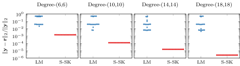
Figure 1: The residual norm of the rational approximation from twenty different initializations computed using Levenberg-Marquardt (LM) applied to Eq. 3 and the Stabilized SK iteration (S-SK) introduced here. In this example, we approximate $|x|$ on $[-1,1]$ using 200,000 equispaced spaced points. The initial numerator and denominator polynomials, both of degree $m$, take normally distributed values with zero mean and unit variance on $m+1$ equispaced points on $[-1,1]$.

1.1 The SK Iteration

Sanathanan and Koerner’s key contribution was to introduce a weight into the linearized rational approximation problem Eq. 4 to better reflect the original rational approximation problem Eq. 2. At the $\ell+1$th iteration, they include the weight $\operatorname{diag}({\mathbf{Q}}{\mathbf{b}}^{\ell})^{-1}$ (the previous iterate’s denominator) and compute new coefficients ${\mathbf{a}}^{\ell+1}$ and ${\mathbf{b}}^{\ell+1}$ solving the approximation problem

(5) $$~{}\operatorname{diag}({\mathbf{Q}}{\mathbf{b}}^{\ell})^{-1}{\mathbf{P}}{\mathbf{a}}^{\ell+1}\approx\operatorname{diag}({\mathbf{Q}}{\mathbf{b}}^{\ell})^{-1}\operatorname{diag}({\mathbf{y}}){\mathbf{Q}}{\mathbf{b}}^{\ell+1}.$$

If ${\mathbf{a}}^{\ell}\to{\mathbf{a}}^{\star}$ and ${\mathbf{b}}^{\ell}\to{\mathbf{b}}^{\star}$, then this limit is a rational approximation of ${\mathbf{y}}$:

(6) $$\operatorname{diag}({\mathbf{Q}}{\mathbf{b}}^{\star})^{-1}{\mathbf{P}}{\mathbf{a}}^{\star}\approx{\mathbf{y}}.$$

If we approximate in a least-squares sense, solving Eq. 5 corresponds to

(7) $${\mathbf{a}}^{\ell+1},{\mathbf{b}}^{\ell+1}\leftarrow\operatorname*{argmin}_{\begin{subarray}{c}{\mathbf{a}},{\mathbf{b}}\\ {\mathbf{b}}\neq{\mathbf{0}}\end{subarray}}\left\|\operatorname{diag}({\mathbf{Q}}{\mathbf{b}}^{\ell})^{-1}\begin{bmatrix}{\mathbf{P}}&-\operatorname{diag}({\mathbf{y}}){\mathbf{Q}}\end{bmatrix}\begin{bmatrix}{\mathbf{a}}\\ {\mathbf{b}}\end{bmatrix}\right\|_{2}$$

which we solve using the singular value decomposition (SVD). The primary challenge with the SK iteration is even if ${\mathbf{P}}$ and ${\mathbf{Q}}$ have condition number one, the weighting can cause this system to be ill-conditioned and consequently yield poor approximations as illustrated in Fig. 2.

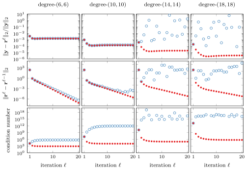
Figure 2: Iteration histories for approximating $|x|$ on $[-1,1]$ using 200,000 equispaced points using the SK iteration. Hollow dots show the standard SK iteration using the Arnoldi basis with condition number one; the solid dots show the Stabilized SK iteration; ${\mathbf{r}}^{\ell}$ is the rational approximation evaluated at $\{x_{j}\}_{j=1}^{M}$ on the $\ell$th iteration; the bottom row refers to the condition number of the smallest right singular vector of the system in Eq. 7 or Eq. 11; see, e.g., [17, Chap. 3, eq. (3.16)].

1.2 Stabilizing the SK Iteration

We correct the ill-conditioning of the SK iteration by building ${\mathbf{P}}$ and ${\mathbf{Q}}$ using a weighted Arnoldi iteration. Recall the Arnoldi iteration builds an orthonormal basis for the for the Krylov subspace

(8) $${\mathcal{K}}_{m}({\mathbf{A}},{\mathbf{w}})=\operatorname{Span}\left\{{\mathbf{w}},{\mathbf{A}}{\mathbf{w}},{\mathbf{A}}^{2}{\mathbf{w}},\ldots,{\mathbf{A}}^{m-1}{\mathbf{w}}\right\}$$

by applying Gram-Schmidt to produce orthonormal vectors ${\mathbf{q}}_{\ell}$ from the sequence ${\mathbf{v}}_{1}={\mathbf{w}}$ and ${\mathbf{v}}_{\ell}\leftarrow{\mathbf{A}}{\mathbf{q}}_{\ell-1}$. If use the Arnoldi iteration to construct a basis for

(9) $${\mathcal{K}}_{m+1}(\operatorname{diag}({\mathbf{x}}),{\mathbf{1}})=\operatorname{Span}\left\{\begin{bmatrix}1\\ \vdots\\ 1\end{bmatrix},\begin{bmatrix}x_{1}\\ \vdots\\ x_{M}\end{bmatrix},\begin{bmatrix}x_{1}^{2}\\ \vdots\\ x_{M}^{2}\end{bmatrix},\cdots,\begin{bmatrix}x_{1}^{m}\\ \vdots\\ x_{M}^{m}\end{bmatrix}\right\}$$

we have constructed an orthonormal basis on $\{x_{j}\}_{j=1}^{M}$ for polynomials of degree $m$. This technique is called Vandermonde with Arnoldi [5] and accurately computes a discrete polynomial basis while avoiding the ill-conditioning of standard Vandermonde matrices [14]. Here we use this insight to construct an orthonormal basis with respect to weighting at each step of the SK iteration. If ${\mathbf{V}}_{m}\in\mathbb{C}^{M\times(m+1)}$ is a basis for ${\mathcal{P}}_{m}$ on $\{x_{j}\}_{j=1}^{M}$, then $\operatorname{Range}({\mathbf{V}}_{m})={\mathcal{K}}_{m+1}(\operatorname{diag}({\mathbf{x}}),{\mathbf{1}})$ and

(10) $$\operatorname{Range}(\operatorname{diag}({\mathbf{w}}){\mathbf{V}}_{m})=\operatorname{Span}\left\{\operatorname{diag}({\mathbf{w}})\begin{bmatrix}x_{1}^{k}\\ \vdots\\ x_{M}^{k}\end{bmatrix}\right\}_{k=0}^{m}={\mathcal{K}}_{m+1}(\operatorname{diag}({\mathbf{x}}),{\mathbf{w}}).$$

By choosing the initial vector ${\mathbf{w}}^{\ell}$ to be the inverse of the previous iterate’s denominator, $w_{j}^{\ell}=1/q_{\ell-1}(x_{j})$, we can then construct iteration-dependent bases ${\mathbf{P}}^{\ell}$ and ${\mathbf{Q}}^{\ell}$ using Vandermonde with Arnoldi. As these bases implicitly include the weight, we can update the polynomial coefficients by solving

(11) $${\mathbf{a}}^{\ell},{\mathbf{b}}^{\ell}\leftarrow\min_{\begin{subarray}{c}{\mathbf{a}},{\mathbf{b}}\\ {\mathbf{b}}\neq 0\end{subarray}}\left\|\begin{bmatrix}{\mathbf{P}}^{\ell}&-\operatorname{diag}({\mathbf{y}}){\mathbf{Q}}^{\ell}\end{bmatrix}\begin{bmatrix}{\mathbf{a}}\\ {\mathbf{b}}\end{bmatrix}\right\|_{2}.$$

Unlike the standard SK iteration Eq. 7, this problem tends to be well-conditioned and often converges linearly to its fixed points as seen in Fig. 2. As the same weight appears in both the numerator and denominator, we can evaluate the rational approximation on $\{x_{j}\}_{j=1}^{M}$ by simply computing $\operatorname{diag}({\mathbf{Q}}^{\ell}{\mathbf{b}}^{\ell})^{-1}{\mathbf{P}}^{\ell}{\mathbf{a}}^{\ell}$. However to evaluate the denominator when computing the initial vector ${\mathbf{w}}^{\ell}$, we must undo the action of the previous weight: $q_{\ell-1}(x_{j})=[{\mathbf{Q}}^{\ell-1}{\mathbf{b}}^{\ell-1}]_{j}/w_{j}^{\ell-1}$. This new Stabilized Sanathanan-Koerner iteration is summarized in Algorithm 1.

Input : Data $\{x_{j},y_{j}\}_{j=1}^{M}$, degrees $m$, $n$ Output : ${\mathbf{R}}_{\mathbf{P}}^{\ell}$, ${\mathbf{R}}_{\mathbf{Q}}^{\ell}$, ${\mathbf{a}}^{\ell}$, ${\mathbf{b}}^{\ell}$ for $\ell$ minimizing $\|{\mathbf{y}}-\operatorname{diag}({\mathbf{Q}}^{\ell}{\mathbf{b}}^{\ell})^{-1}{\mathbf{P}}^{\ell}{\mathbf{a}}^{\ell}\|_{2}$ 1 ${\mathbf{w}}^{0}\leftarrow{\mathbf{1}}$; 2 for $\ell=0,1,2,\ldots$ and not converged do 3       ${\mathbf{P}}^{\ell},{\mathbf{R}}_{\mathbf{P}}^{\ell}\leftarrow$ Arnoldi for ${\mathcal{K}}_{m+1}(\operatorname{diag}({\mathbf{x}}),{\mathbf{w}}^{\ell})$ or Algorithm 2 if multivariate; 4       ${\mathbf{Q}}^{\ell},{\mathbf{R}}_{\mathbf{Q}}^{\ell}\leftarrow$ Arnoldi for ${\mathcal{K}}_{n+1}(\operatorname{diag}({\mathbf{x}}),{\mathbf{w}}^{\ell})$ or Algorithm 2 if multivariate; 5       ${\mathbf{a}}^{\ell},{\mathbf{b}}^{\ell}\leftarrow\min_{{\mathbf{a}},{\mathbf{b}}}\|{\mathbf{P}}^{\ell}{\mathbf{a}}-\operatorname{diag}({\mathbf{y}}){\mathbf{Q}}^{\ell}{\mathbf{b}}\|_{2}$ s.t. $\|{\mathbf{a}}\|_{2}^{2}+\|{\mathbf{b}}\|_{2}^{2}=1$; 6       $[{\mathbf{w}}^{\ell+1}]_{j}\leftarrow w_{j}^{\ell}/[{\mathbf{Q}}^{\ell}{\mathbf{b}}^{\ell}]_{j}$; 7       8

Algorithm 1 Stabilized Sanathanan-Koerner Iteration

1.3 Advantages

The main utility of the Stabilized SK iteration comes in its use for multivariate rational approximation. The only modification required is to replace the use of Vandermonde with Arnoldi to construct discrete polynomial bases ${\mathbf{P}}^{\ell}$ and ${\mathbf{Q}}^{\ell}$ with the corresponding multivariate generalization developed in [2, Subsec. 3.2]. The rational approximations generated by the Stabilized SK iteration often have a least-squares residual norm an order of magnitude smaller than both Parametric-AAA (p-AAA) [6] and the linearized approach advocated in [2, Subsec. 3.1]; moreover the Stabilized SK iteration avoids the spurious poles often encountered in other algorithms (Section 4.2). Additionally, the Stabilized SK places no restriction on the points $\{{\mathbf{x}}_{j}\}_{j=1}^{M}\subset\mathbb{C}^{d}$, unlike p-AAA which requires points on a tensor-product grid.

Applied to univariate rational approximation problems, the Stabilized SK iteration yields comparable approximations to Vector Fitting (Section 4.1). These approximations often have a far smaller least-squares residual norm than those generated by AAA and the linearized approach.

1.4 Disadvantages

Unfortunately the Stabilized SK iteration inherits some limitations of the original SK iteration: fixed points of this iteration are not least squares optimal [18, Subsec. 5.2], the iteration can cycle (this happens for odd degrees in the example from Fig. 2), and iterates do not monotonically decrease the least-squares residual norm as seen in Fig. 2. We address the last two issues by performing only a few iterations (typically twenty) and returning the best rational approximation. The first issue tends not to be significant in practice. As residual of the rational approximation decreases, fixed points of the SK iteration approach those of the least squares problem. Often we see in our examples that refining rational approximation using nonlinear least squares only slightly decreases the residual norm.

The Stabilized SK iteration is more expensive than other algorithms due to the need to perform two orthogonalizations at each step. However, this does not increase the asymptotic complexity; each of AAA, SK, Stabilized SK, and Vector Fitting require $\mathcal{O}(MN^{2})$ operations where $N$ is the number of columns in ${\mathbf{P}}$ and ${\mathbf{Q}}$.

1.5 Outline

In the remainder of this paper we first review the multivariate Vandermonde with Arnoldi algorithm introduced in [2] and extend it for total-degree polynomials (Section 2). We then briefly discuss implementation details for refining rational approximations using nonlinear least squares techniques (Section 3). Finally, we conclude with several numerical examples comparing the Stabilized SK iteration to other rational approximation techniques on both univariate and multivariate test problems (Section 4).

1.6 Reproducibility

Following the principles of reproducible research, we provide software implementing the algorithms in this paper and scripts generating the figures at https://github.com/jeffrey-hokanson/polyrat.

2 Multivariate Vandermonde with Arnoldi

We extend the univariate Stabilized Sanathanan-Koerner iteration to multivariate rational approximation,

(12) $$y_{j}\approx r_{j}=r({\mathbf{x}}_{j})\coloneqq\frac{p({\mathbf{x}}_{j})}{q({\mathbf{x}}_{j})}\quad\text{where}\quad\{{\mathbf{x}}_{j}\}_{j=1}^{M}\subset\mathbb{C}^{d}\quad\text{and}\quad p,q\text{ polynomials},$$

by replacing Vandermonde with Arnoldi with its multivariate extension developed in [2, Subsec. 3.2]. Here consider two classes of multivariate polynomials: total degree polynomials ${\mathcal{P}}^{\text{tot}}_{m}$ and maximum degree polynomials ${\mathcal{P}}_{{\mathbf{m}}}^{\text{max}}$,

(13) $${\mathcal{P}}_{m}^{\text{tot}} \coloneqq\operatorname{Span}\left\{f:f({\mathbf{x}})=\prod_{i=1}^{d}x_{i}^{\alpha_{i}}\right\}_{|{\boldsymbol{\alpha}}|\leq m}, \quad|{\boldsymbol{\alpha}}|=\sum_{i=1}^{d}\alpha_{i};$$ where

(14) $${\mathcal{P}}_{{\mathbf{m}}}^{\text{max}} \coloneqq\operatorname{Span}\left\{f:f({\mathbf{x}})=\prod_{i=1}^{d}x_{i}^{\alpha_{i}}\right\}_{{\boldsymbol{\alpha}}\leq{\mathbf{m}}}, \quad{\boldsymbol{\alpha}}\leq{\mathbf{m}}\Leftrightarrow\alpha_{i}\leq m_{i}.$$ where

The main difference in the multivariate extension of Vandermonde with Arnoldi is that the basis no longer corresponds to a Krylov subspace. Instead we generate new columns by carefully selecting one coordinate of the points $\{{\mathbf{x}}_{j}\}_{j=1}^{M}$ to multiply by a proceeding column and then apply Gram-Schmidt as before. Here we briefly provide the details on constructing this basis and evaluating this basis at new points.

2.1 Building a Basis

Our goal will be to find an ordering of multi-indices ${\mathcal{I}}$ appearing in the polynomial basis definition in Eqs. 13 and 14 such that the columns ${\mathbf{q}}_{1},\ldots,{\mathbf{q}}_{\ell}$ generated by multivariate Vandermonde with Arnoldi satisfy

(15) $$\operatorname{Span}\{{\mathbf{q}}_{k}\}_{k=1}^{\ell}=\operatorname{Span}\left\{\begin{bmatrix}{\mathbf{x}}_{1}^{{\boldsymbol{\alpha}}}\\ \vdots\\ {\mathbf{x}}_{M}^{{\boldsymbol{\alpha}}}\end{bmatrix}\right\}_{{\boldsymbol{\alpha}}\in{\mathcal{I}}[1:\ell]},\quad\text{where}\quad{\mathbf{x}}^{{\boldsymbol{\alpha}}}=\prod_{i=1}^{d}x_{i}^{\alpha_{i}}.$$

At each step of multivariate Vandermonde with Arnoldi, we generate the next column ${\mathbf{v}}_{\ell+1}$ to orthogonalize against ${\mathbf{q}}_{1},\ldots,{\mathbf{q}}_{\ell}$ by multiplying ${\mathbf{q}}_{k}$ by the $j$th:

(16) $${\mathbf{v}}_{\ell+1}=\operatorname{diag}\left(\begin{bmatrix}[{\mathbf{x}}_{1}]_{j}\\ \vdots\\ [{\mathbf{x}}_{M}]_{j}\end{bmatrix}\right){\mathbf{q}}_{k}.$$

We choose $j$ and $k$ by finding the smallest $k$ such that ${\mathcal{I}}[k]+{\mathbf{e}}_{j}={\mathcal{I}}[\ell+1]$ where ${\mathbf{e}}_{j}$ is the $j$th column of the $d\times d$ identity matrix. With this update rule, we need to pick an ordering ${\mathcal{I}}$ such that Eq. 15 is satisfied; many orderings do not satisfy this constraint! For total degree polynomials a grevlex ordering (ordered by total degree and then lexicographically) satisfies this constraint; i.e.,

$${\mathcal{I}}_{3}^{\text{tot}}=\left[(0,0),(1,0),(0,1),(2,0),(1,1),(0,2),(3,0),(2,1),(1,2),(0,3)\right].$$

For maximum degree polynomials we satisfy this constraint using a lexicographic ordering; i.e.,

$${\mathcal{I}}_{(2,2)}^{\text{max}}=\left[(0,0),(0,1),(0,2),(1,0),(1,1),(1,2),(2,0),(2,1),(2,2)\right].$$

Algorithm 2 summarizes the multivariate Vandermonde with Arnoldi process. In our implementation we use classical Gram-Schmidt with two steps of iterative refinement [4, Sec. 6] rather than modified Gram-Schmidt. Although this uses more floating point operations, classical Gram-Schmidt allows us to make use of BLAS level 2 operations yielding a net decrease in wall-clock time compared to the BLAS level 1 operations used in modified Gram-Schmidt.

Input :  $\{{\mathbf{x}}_{j}\}_{j=1}^{M}\subset\mathbb{C}^{d}$, weight ${\mathbf{w}}$ index set ${\mathcal{I}}$ of length $N$ Output :  ${\mathbf{Q}}\in\mathbb{C}^{M\times N}$, ${\mathbf{R}}\in\mathbb{C}^{N\times N}$ 1 ${\mathbf{Q}}\leftarrow{\mathbf{0}}$, ${\mathbf{R}}\leftarrow{\mathbf{0}}$; 2 $[{\mathbf{R}}]_{1,1}\leftarrow\|{\mathbf{w}}\|_{2}$; 3 $[{\mathbf{Q}}]_{:,1}\leftarrow{\mathbf{w}}/[{\mathbf{R}}]_{1,1}$; 4 for $\ell=2,3,\ldots,|{\mathcal{I}}|$ do 5       Pick smallest $k$ such that $\exists j$ where ${\mathcal{I}}[k]+{\mathbf{e}}_{j}={\mathcal{I}}[\ell]$; 6       ${\mathbf{v}}_{\ell}\leftarrow\operatorname{diag}([[{\mathbf{x}}_{1}]_{j},\cdots,[{\mathbf{x}}_{M}]_{j}]){\mathbf{q}}_{k}$; 7       for $t=1,2$ do 8             ${\mathbf{s}}\leftarrow[{\mathbf{Q}}]_{\cdot,1:\ell-1}^{*}{\mathbf{v}}_{\ell}$; 9             ${\mathbf{v}}_{\ell}\leftarrow{\mathbf{v}}_{\ell}-[{\mathbf{Q}}]_{\cdot,1:\ell-1}{\mathbf{s}}$; 10             $[{\mathbf{R}}]_{1:\ell-1,\ell}\leftarrow[{\mathbf{R}}]_{1:k-1,k}+{\mathbf{s}}$; 11             12      $[{\mathbf{R}}]_{\ell,\ell}\leftarrow\|{\mathbf{v}}_{\ell}\|_{2}$; 13       $[{\mathbf{Q}}]_{:,\ell}\leftarrow{\mathbf{v}}_{\ell}/[{\mathbf{R}}]_{\ell,\ell}$; 14      

Algorithm 2 Multivariate Vandermonde with Arnoldi

2.2 Evaluating a Basis

Once we have constructed a polynomial basis in Algorithm 2, we need to be able to evaluate the resulting basis at new points ${\mathbf{z}}\in\mathbb{C}^{d}$. To do so, we simply repeat the construction as before but keep ${\mathbf{R}}$ fixed as illustrated in Algorithm 3.

Input :  $\{{\mathbf{z}}_{j}\}_{j=1}^{M}\subset\mathbb{C}^{d}$, index set ${\mathcal{I}}$ of length $N$, ${\mathbf{R}}\in\mathbb{C}^{N\times N}$ Output :  ${\mathbf{W}}\in\mathbb{C}^{M\times N}$ 1 $[{\mathbf{W}}]_{\cdot,1}\leftarrow{\mathbf{1}}/[{\mathbf{R}}]_{1,1}$; 2 for $\ell=2,3,\ldots,|{\mathcal{I}}|$ do 3       Pick smallest $k$ such that $\exists j$ where ${\mathcal{I}}[k]+{\mathbf{e}}_{j}={\mathcal{I}}[\ell]$; 4       ${\mathbf{v}}_{\ell}\leftarrow\operatorname{diag}([[{\mathbf{z}}_{1}]_{j},\ldots,[{\mathbf{z}}_{M}]_{j}]){\mathbf{q}}_{j}$; 5       ${\mathbf{v}}_{\ell}\leftarrow{\mathbf{v}}_{\ell}-[{\mathbf{W}}]_{\cdot,1:\ell-1}[{\mathbf{R}}]_{1:\ell-1,\ell}$; 6       $[{\mathbf{W}}]_{\cdot,\ell}\leftarrow{\mathbf{v}}_{\ell}/[{\mathbf{R}}]_{\ell,\ell}$; 7      

Algorithm 3 Evaluating a Vandermonde with Arnoldi Basis at New Points

3 Refinement to Local Optimality

In some situations we desire locally optimal rational approximations; namely, ${\mathbf{a}}^{\star}$ and ${\mathbf{b}}^{\star}$ satisfying the first order necessary conditions of

(17) $$\min_{{\mathbf{a}},{\mathbf{b}}}\|{\mathbf{f}}({\mathbf{a}},{\mathbf{b}})\|_{2},\quad\text{where}\quad{\mathbf{f}}({\mathbf{a}},{\mathbf{b}})\coloneqq{\mathbf{y}}-\operatorname{diag}({\mathbf{Q}}{\mathbf{b}})^{-1}{\mathbf{P}}{\mathbf{a}}.$$

Although the best iterate of the Stabilized SK will not satisfy the local optimality conditions, it frequently provides a good initialization for a nonlinear least squares solver. There is only one difficulty in applying standard nonlinear least squares algorithms to the rational approximation problem Eq. 17: the Jacobian of ${\mathbf{f}}$ is structurally rank-deficient. For any scalar $\alpha$, ${\mathbf{f}}({\mathbf{a}},{\mathbf{b}})={\mathbf{f}}(\alpha{\mathbf{a}},\alpha{\mathbf{b}})$. Hence there is one additional degree of freedom if the coefficients ${\mathbf{a}}$ and ${\mathbf{b}}$ are real; two if these coefficients are complex. In our implementation we remove this rank deficiency by fixing the value of the largest entry in ${\mathbf{b}}$.

An additional concern is that the Jacobian of ${\mathbf{f}}$,

(18) $${\mathbf{F}}({\mathbf{a}},{\mathbf{b}}) =\begin{bmatrix}\operatorname{diag}({\mathbf{Q}}{\mathbf{b}})^{-1}{\mathbf{P}}&-\operatorname{diag}[\operatorname{diag}({\mathbf{Q}}{\mathbf{b}})^{-2}{\mathbf{P}}{\mathbf{a}}]{\mathbf{Q}}\end{bmatrix},$$

can be ill-conditioned due to the presence of $\operatorname{diag}({\mathbf{Q}}{\mathbf{b}})^{-1}$ much like the SK iteration. We can partially rectify this by using the basis generated by the $\ell$th step of the Stabilized SK iteration.

4 Numerical Experiments

Here we compare the Stabilized SK iteration to other univariate and multivariate rational approximation algorithms on a series of test problems from recent literature.

4.1 Univariate Problems

Here we consider four univariate rational approximation test problems from Nakatsukasa, Sète, and Trefethen [13] and compare the performance of of AAA [13], vector fitting [10], linearized rational approximation [2], and our Stabilized SK iteration both with and without refinement to local least-squares optimality. These results are shown in Fig. 3. In each case we see that the rational approximation generated by the Stabilized SK iteration yields one of the best approximations with a similar residual norm as to Vector Fitting; both AAA and the linearized approach yield worse approximations. We also observe that refining the Stabilized SK approximation to a local optimizer does not often substantially improve the result. Details on these four examples follows.

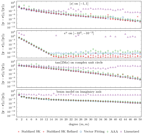
Figure 3: The performance of different rational approximation algorithms on the four univariate rational approximation examples described in Section 4.1. Many of the linearized results for the exponential example are outside the plotting range.

Example 4.1 (Absolute Value).

Approximating $f(x)=|x|$ using 200,000 equispaced points on the interval $[-1,1]$ [13, Subsec. 6.7].

This example challenges each algorithm with a large quantity of data. As the absolute value function is even, we only see improvement when the numerator and denominator degrees are even. Although the Stabilized SK iteration often yields a good rational approximation, there are some cases where this algorithm fails; i.e., degrees 30, 37, and 49. This may be due to extreme ill-conditioning on the first step, as seen in Fig. 2, preventing the algorithm from making further progress.

Example 4.2 (Exponential).

Approximating $f(x)=\exp(x)$ using 2,000 logarithmically spaced points on the interval $[-10^{4},-10^{-3}]$ [13, Subsec. 6.8].

This example challenges each algorithm to handle points separated by seven orders of magnitude. Each algorithm except for the linearized rational approximation performs well in this example. The linearized approach breaks down because the denominator it identifies has a near zero-value at every point.

Example 4.3 (Tangent).

Approximating $f(x)=\tan(256x)$ using 1000 equispaced points on the unit circle [13, Subsec. 6.3].

This example illustrates behavior using complex-valued points $x_{j}$ and responses $y_{j}$. AAA exhibits some oscillations in the accuracy of its approximation whereas the Stabilized SK iteration (especially after refinement) converges smoothly.

Example 4.4 (Beam).

Approximating the beam model [7] (a rational function of degree $(347,348)$) using 1000 points on the imaginary axis with 500 logarithmically spaced points between $10^{-2}i$ and $10^{2}i$ and their complex conjugates [13, Subsec. 6.9].

This example provides a system identification application of rational approximation. There is no clear best algorithm among Stabilized SK, AAA, and Vector Fitting, although the overall trend is similar.

4.2 Spurious Poles

A concern with both AAA [13, Sec. 5] and the linearized rational approximation [2, Subsec. 3.3] is the appearance of Froissart doublets—poles of the rational approximation with a near-zero residue contributing little to the approximation. Some Froissart doublets are numerical artifacts of the fitting procedure; others occur even in exact arithmetic as in the absolute value test case (example 4.1) where every odd degree approximation has one pole with zero residue. Froissart doublets rarely appear in the rational approximations produced by the Stabilized SK iteration in our experience. Fixed points of the SK iteration are often nearby least-squares local minimizers and these local minimizers are unlikely to have poles with a near-zero residue as they would contribute little to reducing the residual. The following example appearing in Fig. 4 illustrates this point.

Example 4.5.

Approximating

(19) $$f(x_{1},x_{2})=\frac{\exp(x_{1}x_{2})}{(x_{1}-1.2)(x_{1}+1.2)(x_{2}-1.2)(x_{2}+1.2)}\quad\text{on}\quad{\mathbf{x}}\in[-1,1]^{2}$$

using 1000 randomly distributed points with uniform probability [2, Subsec. 3.3].

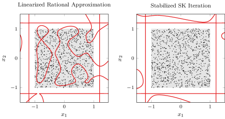
Figure 4: The Stabilized SK iteration avoids spurious poles unlike linearized rational approximation. Here we approximate Example 4.5 by a rational function of total degree-$(20,20)$ and show zeros of the denominator (lines), points used to construct the approximation (dots), and the region of approximation (shaded square); cf. [2, Fig. 1].

In this example we expect the rational approximation to be analytic on $[-1,1]^{2}$ and have poles at $x_{1}=\pm 1.2$ and $x_{2}=\pm 1.2$. In Fig. 4 we see that the linearized approach introduces spurious zeros inside the approximation domain $[-1,1]^{2}$ whereas the Stabilized SK iteration avoids these for the same degree rational approximation.

4.3 Parametric Transfer Function Approximation

One important application of multivariate rational approximation is parametric model reduction. In this setting we have a transfer function $H$ that depends on both frequency $z\in\mathbb{C}$ and some parameters ${\mathbf{t}}$, typically real:

(20) $$H(z,{\mathbf{t}})={\mathbf{c}}^{*}(z{\mathbf{I}}-{\mathbf{A}}({\mathbf{t}}))^{-1}{\mathbf{b}}.$$

In this context we seek a max-degree rational approximations as the degree in $z$ is typically much higher than in the parameters ${\mathbf{t}}$. Here we consider two variants of the Penzl model [15, Ex. 3]: one with one parameter, the other with two.

Example 4.6 (One Parameter Penzl Model).

Consider a one parameter variant of the Penzl model [11, Subsec. 5.2]

(21) $$H(z,t) ={\mathbf{c}}^{\top}\left[z{\mathbf{I}}-\operatorname{diag}({\mathbf{A}}_{1}(t),{\mathbf{A}}_{2},{\mathbf{A}}_{3},{\mathbf{A}}_{4})\right]^{-1}{\mathbf{b}}\quad\text{with}$$

(22) $${\mathbf{A}}_{1}(t) =\begin{bmatrix}-1&t\\ -t&-1\end{bmatrix},\ {\mathbf{A}}_{2}=\begin{bmatrix}-1&200\\ -200&-1\end{bmatrix},\ {\mathbf{A}}_{3}=\begin{bmatrix}-1&400\\ -400&-1\end{bmatrix},$$

${\mathbf{A}}_{4}=-\operatorname{diag}(1,2,\ldots,1000)$, and ${\mathbf{b}}={\mathbf{c}}=[\overbrace{10\cdots 10}^{6}\overbrace{1\cdots 1}^{1000}]$. We seek to approximate $H$ where $z\in[0.1,1000]i$ and $t\in[10,100]$ using a tensor product grid with 100 logarithmically spaced points in $z$ and 30 uniformly spaced points in $t$ [6, Subsec. 3.2.3].

Figure 5 shows the point-wise error of the multivariate rational approximations produced by linearized rational approximation [2], Parametric-AAA [6], and our Stabilized SK iteration. In this case the Stabilized SK iteration produces an approximation that is accurate throughout the domain whereas the p-AAA approximation is most accurate near its interpolation points and the linearized approximation is only accurate for large $z$. Note the least squares residual norm of Stabilized SK is approximately one tenth that of p-AAA and approximately one hundredth that of the linearized approach.

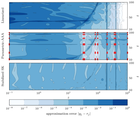
Figure 5: The error in rational approximations of of total degree $([8,8],[8,8])$ on the one-parameter Penzl model with two variables described in Example 4.6. Dots denote the p-AAA interpolation points. The least squares residual norm on the training data is $2.203$ for linearized rational approximation, $0.238$ for p-AAA, and $0.0189$ for Stabilized SK.

Example 4.7 (Two Parameter Penzl Model).

Consider a two parameter variant of the Penzl model [6, Subsec. 3.3.1]

(23) $$H(z,t,u) ={\mathbf{c}}^{\top}\left[z{\mathbf{I}}-\operatorname{diag}({\mathbf{A}}_{1}(t),{\mathbf{A}}_{2}(u),{\mathbf{A}}_{3}(u),{\mathbf{A}}_{4})\right]^{-1}{\mathbf{b}}\text{ with}$$

(24) $${\mathbf{A}}_{2}(u) =\begin{bmatrix}-1&u\\ -u&-1\end{bmatrix},\ {\mathbf{A}}_{3}(u)=\begin{bmatrix}-1&2u\\ -2u&-1\end{bmatrix}$$

with the remainder of the variables are as defined in Example 4.6. We approximate $H$ for $z\in[1,2000]i$, $t\in[10,100]$, and $u\in[150,250]$ using a tensor product grid with $100$ logarithmically spaced frequencies in $z$ and $10$ equispaced points in $t$ and $u$.

Table 1: A performance comparison of linearized rational approximation, Parametric-AAA, and Stabilized SK on the two parameter Penzl model (example 4.7) using the total degrees generated by iterates of p-AAA.

numerator			denominator			$\|{\mathbf{y}}-{\mathbf{r}}\|_{2}/\|{\mathbf{y}}\|_{2}$
$z$	$t$	$u$	$z$	$t$	$u$	Linearized		Parametric-AAA		Stabilized SK
$6$	$6$	$4$	$6$	$6$	$4$	$1$	$.7457\cdot 10^{-2}$	$4$	$.8495\cdot 10^{-2}$	$1$	$.0519\cdot 10^{-3}$
$7$	$6$	$5$	$7$	$6$	$5$	$1$	$.5665\cdot 10^{-2}$	$1$	$.7257\cdot 10^{-2}$	$2$	$.4642\cdot 10^{-4}$
$8$	$7$	$5$	$8$	$7$	$5$	$5$	$.5283\cdot 10^{-3}$	$1$	$.0156\cdot 10^{-3}$	$5$	$.0861\cdot 10^{-4}$
$9$	$7$	$6$	$9$	$7$	$6$	$1$	$.0274\cdot 10^{-3}$	$2$	$.1641\cdot 10^{-4}$	$9$	$.3558\cdot 10^{-5}$
$10$	$7$	$6$	$10$	$7$	$6$	$6$	$.9173\cdot 10^{-4}$	$2$	$.6580\cdot 10^{-5}$	$7$	$.2155\cdot 10^{-7}$
$11$	$7$	$6$	$11$	$7$	$6$	$6$	$.1594\cdot 10^{-4}$	$2$	$.8536\cdot 10^{-6}$	$2$	$.0291\cdot 10^{-7}$
$12$	$8$	$7$	$12$	$8$	$7$	$5$	$.0109\cdot 10^{-3}$	$5$	$.0087\cdot 10^{-6}$	$1$	$.7921\cdot 10^{-8}$

Table 1 shows the history of rational approximations generated by Parametric-AAA for the two parameter Penzl model and the corresponding residual norms for both linearized rational approximation and the Stabilized SK iteration. This example shows the Stabilized SK iteration produces an approximation with a smaller residual norm, often by an order of magnitude or more.

5 Discussion

Here we corrected the numerical instability in the Sanathanan-Koerner iteration exposing a practical algorithm for univariate and multivariate rational approximations. Although not optimal, this algorithm yields excellent rational approximations. Here we have only considered scalar-valued rational approximation problems, however we could extend the Stabilized Sanathanan-Koerner iteration to vector- and matrix-valued rational approximation following [8, subsec. 2.4].

References

- [1] A. C. Antoulas and B. D. Q. Anderson, On the scalar rational interpolation problem, IMA Journal of Mathematical Control & Information, 3 (1986), pp. 61–88, https://doi.org/10.1093/imamci/3.2-3.61.
- [2] A. P. Austin, M. Krishnamoorthy, S. Leyffer, S. Mrenna, J. Müller, and H. Schulz, Multivariate rational approximation, 2019, https://arxiv.org/abs/1912.02272v1.
- [3] J.-P. Berrut and L. N. Trefethen, Barycentric Lagrange interpolation, SIAM Rev., 46 (2004), pp. 501–517, https://doi.org/10.1137/S0036144502417715.
- [4] Å. Björck, Numerics of Gram-Schmidt orthogonalization, Linear Algebra and its Applications, 198 (1994), pp. 297–316, https://doi.org/10.1016/0024-3795(94)90493-6.
- [5] P. D. Brubeck, Y. Nakatsukasa, and L. N. Trefethen, Vandermonde with Arnoldi, 2019, https://arxiv.org/abs/1911.099988v1.
- [6] A. Carracedo Rodriguez and S. Gugercin, The p-AAA algorithm for data driven modeling of parameteric dynamical systems, 2020, https://arxiv.org/abs/2003.06536v2.
- [7] Y. Chahlaoui and P. V. Dooren, A collection of benchmark examples for model reduction of linear time invariant dynamical systems, Tech. Report 2, SLICOT, Feb. 2002.
- [8] Z. Drmač, S. Gugercin, and C. Beattie, Vector fitting for matrix-valued rational approximation, SIAM J. Sci. Comput., 37 (2015), pp. A2346–A2379, https://doi.org/10.1137/15M1010774.
- [9] B. Gustavsen, Improving the pole relocating properties of vector fitting, IEEE T. Power Deliv., 21 (2006), pp. 1587–1592, https://doi.org/10.1109/TPWRD.2005.860281.
- [10] B. Gustavsen and A. Semlyen, Rational approximation of frequency domain responses by vector fitting, IEEE T. Power Deliv., 14 (1999), pp. 1052–1061.
- [11] A. C. Ionita and A. C. Antoulas, Data-driven parametrized model reduction in the Loewner framework, SIAM J. Sci. Comput., 36, pp. A984–A1007, https://doi.org/10.1137/130914619.
- [12] E. C. Levy, Complex-curve fitting, IRE Trans. Autom. Control, 4 (1959), pp. 37–43, https://doi.org/10.1109/TAC.1959.6429401.
- [13] Y. Nakatsukasa, O. Sète, and L. N. Trefethen, The AAA algorithm for rational approximation, SIAM J. Sci. Comput., 40 (2018), pp. A1494–A1522, https://doi.org/10.1137/16M1106122.
- [14] V. Y. Pan, How bad are Vandermonde matrices?, SIAM J. Matrix Anal. A., 37 (2016), pp. 676–694, https://doi.org/10.1137/15M1030170.
- [15] T. Penzl, Algorithms for model reduction of large dynamical systems, Linear Algebra and its Applications, 415 (2006), pp. 322–343, https://doi.org/10.1016/j.laa.2006.01.007.
- [16] C. K. Sanathanan and J. Koerner, Transfer function synthesis as a ratio of two complex polynomials, IEEE T. Automat. Contr., 8 (1963), pp. 56–58, https://doi.org/10.1109/TAC.1963.1105517.
- [17] G. W. Stewart, Matrix Algorithms, SIAM, 2001.
- [18] A. H. Whitfield, Asymptotic behaviour of transfer function synthesis methods, Int. J. Control, 45 (1987), pp. 1083–1092, https://doi.org/10.1080/00207178708933791.