A Hybrid Model for Learning Embeddings
and Logical Rules Simultaneously
from Knowledge Graphs

Abstract

The problem of knowledge graph (KG) reasoning has been widely explored by traditional rule-based systems and more recently by knowledge graph embedding methods. While logical rules can capture deterministic behavior in a KG they are brittle and mining ones that infer facts beyond the known KG is challenging. Probabilistic embedding methods are effective in capturing global soft statistical tendencies and reasoning with them is computationally efficient. While embedding representations learned from rich training data are expressive, incompleteness and sparsity in real-world KGs can impact their effectiveness. We aim to leverage the complementary properties of both methods to develop a hybrid model that learns both high-quality rules and embeddings simultaneously. Our method uses a cross feedback paradigm wherein, an embedding model is used to guide the search of a rule mining system to mine rules and infer new facts. These new facts are sampled and further used to refine the embedding model. Experiments on multiple benchmark datasets show the effectiveness of our method over other competitive standalone and hybrid baselines. We also show its efficacy in a sparse KG setting and finally explore the connection with negative sampling.

I Introduction

Knowledge graphs (KGs) are large directed graphs where nodes represent concrete or abstract entities and edges symbolize relations for a pair of nodes. Many KGs containing millions of entities and relation types exist today viz. Freebase [1], YAGO [2], Wikidata [3], and Google Knowledge Graph [4] which are pivotal in reasoning about multi-relational data from different domains. One important reasoning problem is that of predicting missing relationships between entities (link prediction). Reasoning over KGs is particularly challenging in part due of their characteristic properties: large size, incompleteness, sparsity and noisy facts. Latent feature (a.k.a embedding) models learned probabilistically (RESCAL [5], TransE [6], ComplEx [7] and RotatE [8]) and inductive logic programming (ILP) inspired techniques which mine interpretable logical rules (WARMER [9], AIME+ [10]) are two prominent KG reasoning approaches.

Relations in knowledge graphs adhere to certain constraints which enforce syntactic validity and typically follow deterministic connectivity patterns like equivalence, symmetry, inversion and composition. Rules which capture such patterns are precise, interpretable and can generalize well. Drawbacks includes potential low coverage, mining inefficiency (large search space) and difficulty in mining quality rules from incomplete KGs. Embedding methods aim to learn useful representations of entities and relations by projecting known triplets into low-dimensional vector spaces and maximizing the total plausibility of known facts in the KG. Embedding models are able to capture unobservable but intrinsic and semantic properties of entities and relations [11]. As reasoning with embeddings boils down to vector space calculations it is computationally efficient, but it can be inaccurate when the entities and relations are sparse or noisy. [12].

Since both methods have their advantages and disadvantages, in this paper we propose a hybrid model which aims to exploit their complementary strengths. The main idea is to selectively utilize inferred facts from logical rules for embedding learning. Also, embedding feedback is used to prune the search space of the rule mining system. This cross feedback process when run for many iterations, simultaneously learns to incorporate deterministic structure into embeddings and mine rules that are consistent with “global” KG patterns. Hybrid models proposed previously in the literature use simple logical rules to place constraints on the embedding space in order to incorporate structure. Rule learning is detached from embedding learning and most methods just naively enumerate all possible rules to start with, which doesn’t scale for larger KGs. Methods like IterE [13] place assumptions on the kind of rules and embedding techniques that can be used and are built specifically to tackle sparse entities. Different from such methods, our model aims to simultaneously improve embeddings and mine diverse and reliable rules. Moreover, our method can be incorporated with any embedding technique and rule mining system.

II Background

Let $\mathcal{E}$ represent the set of all entities and $\mathcal{R}$ the set of all relation types in the KG. A knowledge graph $G$ contains a set of factual triplets $\{(h,r,t)|h,t\in\mathcal{E};r\in\mathcal{R}\}$. $h,r,t$ are called head, relation and tail respectively. Figure 1 shows a sample from a larger knowledge graph about sports. Knowledge graph reasoning in particular link prediction deals with the problem of inferring new relationships between entities and triplet classification involves predicting the existence of candidate triplets in a given KG.

Knowledge graph embedding Entities are represented as vectors and relations are seen as operations in vector space and are typically represented as vectors, matrices or tensors. These models assume that the existence of individual triplets in a KG are conditionally independent given latent representations a.k.a embeddings of entities and relations in a continuous vector space. A score function $\phi:\mathcal{E}\times\mathcal{R}\times\mathcal{E}\rightarrow\mathbb{R}$ is used to measure the model’s confidence in a candidate triplet and defined based on different vector space assumptions for e.g., a popular model called TransE [6] aims is to have $\mathbf{h}+\mathbf{r}\approx\mathbf{t}$ if $(h,r,t)\in KG$, (boldface letters represent respective embeddings in $\mathbb{R}^{d}$). So, the score function $\phi(h,r,t)=-\|\mathbf{h}+\mathbf{r}-\mathbf{t}\|$ is expected to be large if $(h,r,t)$ exists in the KG . Embedding learning is done under open world assumption (OWA) where un-observed triplets are either false or unknown. Negative sampling is employed due to the lack of negative examples in the input KG. A simple and effective approach [6] is to corrupt either the head or tail of a true triplet with a random entity sampled uniformly from $\mathcal{E}$. Entity and relation embeddings are learned by minimizing logistic or pairwise ranking loss.

TABLE I: State-of-the-art embedding score functions.

Model	Score Function ($\phi$)
TransE	$-\|\mathbf{h}+\mathbf{r}-\mathbf{t}\|$
DistMult	$\langle\mathbf{h},\mathbf{r},\mathbf{t}\rangle$
ComplEx	$\textbf{Re}(\langle\mathbf{h},\mathbf{r},\overline{\mathbf{t}}\rangle)$
RotatE	$-\|\mathbf{h}\circ\mathbf{r}-\mathbf{t}\|$

Rule Mining A rule is a formulae of atoms connected with logical connectives. In particular, a rule is Horn if the conjunction of a set of body atoms results in a single head atom like, $\tau:B_{1}\land B_{2}\land\dots\land B_{n}\rightarrow r(X,Y)$ where $B_{i}$’s are body atoms and $r(X,Y)$ is a head atom. We use $body(\tau)$ to denote the body atoms of rule $\tau$. An instantiation of a rule is the act of substituting all its variables with entities from $\mathcal{E}$. The head atom of an instantiated rule is called an inferred head atom if all body atoms of the instantiated rule exist in the KG. $S_{\tau}$ is the set of all inferred head atoms obtained from the instantiation of a rule $\tau$.

$$S_{\tau}=\{r(X,Y)\mid\exists z_{1},\dots,z_{m}:body(\tau)\}$$ (1)

where $z_{1},\dots,z_{m}$ are variables that appear in the body of the rule. A principled approach to mine horn rules from a KG is by an association rule learning algorithm [14] and [9]. To deal with the vast search space, language biases viz. limiting rule length, having every atom to be transitively connected to each other in a rule (a.k.a connected rules) and ensuring all variables in a rule to to be closed (i.e. appears at least twice) are utilized. During mining, various statistical measures assess the quality of intermediate rules to help prune the search space. According to [14], Rule Support is the number of distinct grounding of the head atom resulting from the body. Formally,

$$supp(\tau)=\#(x,y)\;:\exists z_{1},z_{2},\dots,z_{m}:body(\tau)\land r(x,y)$$ (2)

Standard Confidence (SC) is the ratio of the number of head groundings to the body grounding in the KG.

$$SC(\tau)=\frac{supp(\tau)}{\#(x^{\prime},y^{\prime}):\exists z_{1},z_{2},\dots,z_{m}:body(\tau)}$$ (3)

III Motivation

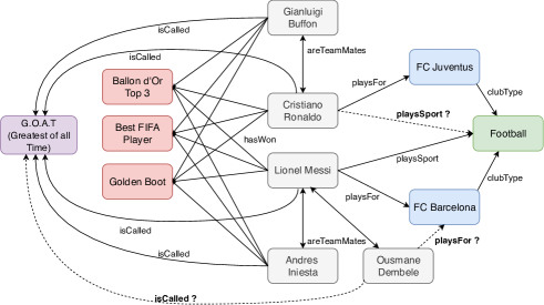
Figure 1: Entities and Relations in $G_{f}$. Known relationships shown as solid edges and possible relations in dashed.

Consider the sample $G_{f}$ in Fig. 1 drawn from a larger KG $G$ about sports. Suppose a rule learning system has found the following three rules:

$$l_{1}:playsFor(V_{1},V_{3})\land clubType(V_{3},V_{2})\rightarrow playsSport(V_{1},V_{2})$$

$$l_{2}:playsFor(V_{1},V_{2})\land playsFor(V_{3},V_{2})\rightarrow teamMate(V_{1},V_{3})$$

$$l_{3}:isCalled(V_{1},V3)\land teamMate(V_{1},V_{2})\rightarrow isCalled(V_{2},V_{3})$$

Q1: Can the generalizing ability of logical rules help embedding methods learn better representations? Rules $l_{1}$ and $l_{2}$ have a number of conforming instantiations in $G_{f}$ and one can argue for them to hold in the larger knowledge graph $G$. Say in a sample pertaining to basketball $G_{b}$, the entities are sparsely connected. Embedding representations of entities in such a “less-connected” sub-graph will not be expressive because of poor data quality. On the other hand, rules $l_{1}$ and $l_{2}$ mined with support from facts in $G_{f}$ can accurately reason about entities in $G_{b}$.

Q2: Can feedback from an embedding model improve the quality of mined rules? Embedding models are good at incorporating global patterns. For example, a possible explanation for Ronaldo being G.O.A.T (greatest of all time) is the presence of a large number of links between him and different sport awards (see Fig. 1). An embedding method say, RESCAL [5] can easily model the pattern: consistent top players of a sport are likely to be called G.O.A.T. Specifically, the model can learn the features of “consistent top player” and “concept of eminence” for different entities from data.

$$\mathbf{h}_{ronaldo}=\begin{bmatrix}0.9\\ 0.1\end{bmatrix}\;\mathbf{M}_{isCalled}=\begin{bmatrix}0.1&0.9\\ 0.1&0.1\end{bmatrix}\;\mathbf{t}_{G.O.A.T}=\begin{bmatrix}0.2\\ 0.9\end{bmatrix}$$

The first embedding feature of $\mathbf{h}$ and $\mathbf{t}$ might model “consistent top player” and the second “concept of eminence”. Thus,

$$\phi\texttt{(ronaldo, isCalled, G.O.A.T)}=\mathbf{h}^{\top}\mathbf{M_{r}}\mathbf{t}=0.76$$

gives a high score denoting validity.

Now, although rule $l_{3}$ has multiple instantiations in $G_{f}$, it is quite noisy and unreliable. For e.g. it will incorrectly infer that Dembele (an upcoming young player) is G.O.A.T by the virtue of him being teammates with Messi. Now, such a noisy rule could have been pruned out if the information from an embedding method modelling consistent top player were to be used. Specifically having,

$$\mathbf{h}_{dembele}=\begin{bmatrix}0.3\\ 0.1\end{bmatrix}$$

$$\phi\texttt{(dembele, isCalled, G.O.A.T)}=\mathbf{h}^{\top}\mathbf{M_{r}}\mathbf{t}=0.26$$

gives a low score showing lower confidence compared to earlier. The two questions raised in the above examples motivates us to develop a cross feedback hybrid model for knowledge base reasoning.

IV Related Work

Here we give a brief overview of embedding learning and rule mining methods and review relevant hybrid models from literature.

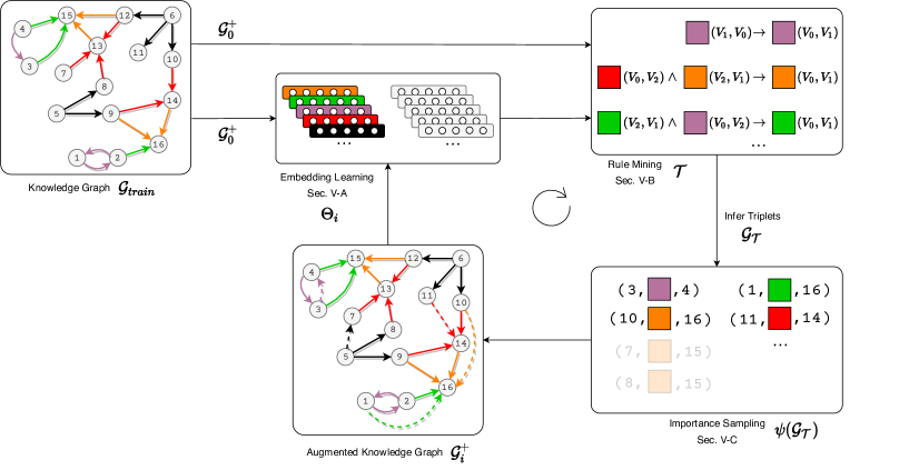
Figure 2: Overall framework architecture.

IV-A Knowledge graph embeddings

RESCAL [5] one of the earliest works in KGE used a bilinear form for the scoring function inspired from matrix factorization. Specifically, $f(h,r,t)=\mathbf{h}^{\top}\mathbf{M_{r}}\mathbf{t}$ where entities $h$ and $t$ are represented by vectors in $\mathbb{R}^{d}$ and relations as matrices in $\mathbb{R}^{d\times d}$ that model pairwise interactions. DistMult [15] simplifies RESCAL further by restricting $\mathbf{M_{r}}$ to be a diagonal matrix . This added simplicity does well for capturing symmetric relationships but bad for others. TransE [6] introduces entity and relation specific embeddings and models them as translations in vector spaces. ComplEx [7] is an extension to DistMult where embedding lie in $\mathbb{C}^{d}$. This accounts for order of the entities and thus is able to model asymmetric relations. A newer method RotatE [8] is able to model symmetry, asymmetry, inversion and composition of relations. It uses the concept of rotations in complex space as opposed to translations in real space. Concretly, $f(h,r,t)=\left\|\mathbf{h}\circ\mathbf{r}-\mathbf{t}\right\|$ with constraint $|r_{i}|=1$ where $\mathbf{h},\mathbf{r},\mathbf{t}\in\mathbb{C}^{d}$ and $\circ$ is the element-wise product. ConvE [16] employs a 2D convolutional neural network to model the score function where the aim is to utilize the expressivity of multiple non-linear features in the architecture to better model relationships in the KG. A comprehensive survey of methods for Knowledge graph embeddings is given in [17] and [18].

IV-B Rule mining

These models assume that existence of a individual triples/facts can be inferred from observable features in the graph usually in the form of logical rules. The extracted rules are then used to infer new facts. Mining rules from a KB has its roots in inductive logic programming (ILP) [19] and association rule mining [20] from the databases community. The use of declarative language biases [21] help in restricting the large search space. Language biases like limiting rule length, having every atom to be transitively connected to each other in a rule (a.k.a connected rules) and ensuring all variables in a rule to to be closed (i.e. appears at least twice) offer a trade-off between the expressivity of rules and size of the search space. WARMR [22] and its extension WARMER [9] is based on the APRIORI algorithm [23] and makes use of a language bias where only conjunctive rules are mined. Sherlock [24] an unsupervised ILP learns first order Horn rules and infers new facts using probabilistic graphical models. To prune the search space it uses two heuristics: statistical significance and relevance. All the above approaches are designed to work under the closed world assumption of KBs due to their treatment of the rule quality measure. AIME [14] and it’s efficient version AIME+ [10] take into account the incompleteness of KBs by proposing a new quality measure based on partial completeness assumption. Additionally they mines Horn rules which are connected, closed, non-reflexive and monotonic (predicates in the rule body are all positive) rules.

IV-C Hybrid Methods

The complementary strengths [25] of observed (rules, paths) and latent (embeddings) KG features has given rise to a number of hybrid models in recent years. In [26] link prediction is cast as an integer linear programming problem in which the objective function is from an embedding model and implication rules are used as constraints. This method is essentially a post processing step which helps in inference but not better embedding representations. Another paradigm of hybrid models is to perform some form of regularization on the embedding loss function using simple rules. In [27] implication rules are first naively extracted by iterating over all possible relation pairs and then differentiable terms are added to the embedding objective function for each grounding of the extracted rules. The naive rule extraction process is costly and the procedure leads to a large number of regularization terms which doesn’t scale. RUGE [28] uses t-norm based fuzzy logic to model the rules and uses inferred triplets to perform embedding rectification. In [29] non-negativity constraints for entity embeddings and entailment constraint for relation embeddings is explored. [30] enforce the subsumption property by having an equality constraint $\mathbf{r_{1}}=\mathbf{r_{2}}-\mathbf{\delta}$, where $\mathbf{\delta}$ is a learnable non-negative vector that specifies how relation $r_{1}$ differs from $r_{2}$. Our work is closest to IterE [13] which is designed for improving embeddings of sparse entities. Seven ontology property axioms from OWL2 Web Ontology Language are used to model relations in the KG. First a pool of valid axioms are generated, by randomly sampling $k$ triples and matching them to seven axiom templates. Then, inferred facts that relate to sparse entities help in learning better embeddings because they essentially provide extra information. We consider horn rules that are more expressive and unlike them, we have no assumptions on the embedding score function. We improve embedding representations of both sparse and non-sparse entities. Different from constraint based hybrid methods, our selective augmentation of inferred facts provides 1) structure to the embedding space and 2) extra information for sparse entities.

V Our Approach

Here, we introduce our hybrid model for learning horn rules and vector space embeddings in a cross feedback paradigm. Initially, embedding learning is performed on the input KG resulting in entity and relation embeddings. The learnt embeddings are then used to guide the rule mining system. Further, the extracted rules are materialized and new inferred triplets are sampled for learning embeddings in the next iteration. Fig. 2 shows the overall framework. In what follows, we describe the three main constituent parts (1) embedding learning, (2) rule learning with embedding feedback and (3) importance sampling of triplets.

V-A Embedding Learning

We associate a label $y_{hrt}$ to each triplet $(h,r,t)$ to model its truth value. Labels of triplets in $G^{+}_{i}$ are set to 1. As there are no negative triplet examples, we generate $G^{-}_{i}$ by negatively sampling $G^{+}_{i}$ and labels of triplets in $G^{-}_{i}$ are set to 0. A score function $\phi(h,r,t;\Theta):\mathcal{E}\times\mathcal{R}\times\mathcal{E}\rightarrow\mathbb{R}$ is used to measure the salience of a triplet $(h,r,t)$. We further map the output of the score function to a continuous truth value between $(0,1)$ using a sigmoid function $\sigma(z)=1/(1+exp(-z))$.

$$\xi(h,r,t)=\sigma(\phi(h,r,t;\Theta))$$ (4)

The objective of embedding learning is to learn $\Theta_{i}$ for iteration $i$ by minimizing the loss over triplets in $G^{+}_{i}$ and $G^{-}_{i}$. $G_{i}=G^{+}_{i}\cup G^{-}_{i}$ represents our learning set for the current iteration $i$. Then,

$$\min_{\Theta_{i}}\frac{1}{|G_{i}|}\sum_{((h,r,t),y_{hrt})\in G_{i}}\mathcal{L}(\xi(h,r,t),y_{hrt})$$ (5)

where $\mathcal{L}(x,y)=-y\log(x)-(1-y)\log(1-x)$ is the cross entropy loss between $x$ and $y$, $\xi(\cdot)$ is the function defined in Eq. 4. It is important to note that in our method, learning is done on an extended set of rule enriched triples. Also, our method does not depend on specific or class of scoring functions unlike IterE [13]. All we require is that the score function $\phi$ output a real valued score. Table I shows the score functions proposed by various state-of-the-art methods in the literature.

V-B Rule Mining with Embedding Feedback

In this step we aim to mine quality horn rules from the set of initial triplets in $G^{+}_{0}$ using the current iteration embeddings $\Theta_{i}$. According to AIME+ [10], rules are modelled as a sequence of atoms with the first atom as the head atom and other body atoms following it. The process of building a quality rule boils down to extending a partial rule sequence and carefully traversing the search space. Rule building is done by a set of mining operators that iteratively add atoms to partial rules until a termination criterion is met. To prune the search space during rule building filtering criteria is utilized. We now explain the three sub parts.

V-B1 Rule Building

Initially, all possible binary atoms using relations in $\mathcal{R}$ are held in a priority queue. These represent partial rule heads with empty bodies. At each iteration of the algorithm, a single partial rule is dequeued and checked for termination (defined below). If successful, it is output as a possible rule. If not, it is extended by each of the following operators:

• Add a new dangling atom ($\mathcal{O}_{D}$) which uses a fresh variable for one argument and a shared variable/entity (used earlier in the rule) for the other.

• Add a new instantiated atom ($\mathcal{O}_{I}$) which uses a shared variable/entity for one argument and an entity for the other.

• Add a new closing atom ($\mathcal{O}_{C}$) which uses shared variable/entity for both arguments.

The expansion produces multiple candidate rules. All candidate rules are checked if they can be pruned by filtering criteria. Pruned ones are discarded and non pruned ones are enqueued for the next iteration. The iterative algorithm is run until the queue is empty.

V-B2 Filtering Criteria

The application of mining operators to a rule produces a set of candidate rules. Since not all candidate rules are promising, this steps aims to filter some of them. Ideally, filtering criteria should allow the generation of rules that (1) explain facts in the KG and (2) infer facts outside the observable KG while being consistent w.r.t global “soft” KG properties. Classical measures of rule quality like standard confidence and PCA confidence introduced by [14] are based on the observable KG. They work well in selecting rules that explain known facts. Every so often, candidate rules infer facts that are outside the known KG and classical measures neglect them. We seek to use the learned embedding as a proxy for measuring the quality of candidate rules which infer facts outside the known KG. This is based on the intuition that embeddings $\Theta$ can capture global statistical patterns. To this end, given a candidate rule, we average the individual embedding scores of all its newly inferred atoms. We call this measure embedding confidence (EC). Given a candidate rule $\tau$, consider the set $S_{\tau}$ defined in Eq. 1. The unobserved facts predicted by instantiating $\tau$ is given by $S_{\tau}\setminus G^{+}_{0}$. Then,

$$\small\begin{split}EC(\tau)&=\frac{1}{|S_{\tau}\setminus G^{+}_{0}|}\sum_{(h,r,t)\in S_{\tau}\setminus G^{+}_{0}}\xi(h,r,t)\end{split}$$ (6)

where $\xi(\cdot)$ is the function defined in Eq. (4). $EC\in(0,1)$ as $\xi(\cdot)$ is designed to give confidence values between $(0,1)$. We consider the weighted average of the classical standard confidence i.e. $SC$ (Eq. 3) and our embedding confidence $EC$ (Eq. 6) for the final rule quality measure $Q$.

$$\small Q(\tau)=(1-\omega)SC(\tau)+\omega EC(\tau)$$ (7)

where $\omega$ the weight factor is a model hyper-parameter. Thus, for each candidate rule we check if there is an increase w.r.t rule quality measure $Q$ and if not it is discarded. Before calculating the $Q$ score for a candidate rule, we use a heuristic pruning strategy followed by AIME+ [14] to discard non-interesting rules. This is done so as to reduce the load on calculating the $Q$ score. One quick statistical check we perform is to make sure a candidate rule covers more than 1% of known facts using head coverage [14]. We also incorporate language biases like restricting the search to rules of length three in order to deal with the vast search space.

Termination Criteria As the extension operators produce rules that are not necessarily closed, we follow [14] in outputting only closed and connected rules.

V-C Importance Sampling of Triplets

Once the rule mining system has extracted rules with a our quality measure, we now incorporate them in refining the embeddings for the next iteration. To do so, the first task is to select top-K rules by ranking the extracted rules according to their quality measure $Q$ which is already calculated (Eq. 7). Let $\mathcal{T}$ represent the set of all the selected rules. Then, the newly inferred triplets from the rules in $\mathcal{T}$ will be represented by,

$$\small G_{\mathcal{T}}=(\bigcup\limits_{\tau\in\mathcal{T}}S_{\tau})\setminus G^{+}_{0}$$ (8)

where $S_{\tau}$ (Eq. 1) is the set of inferred triplets from rule $\tau$. Next we augment the current positive triplet set $G^{+}_{i}$ with $G_{\mathcal{T}}$ to create $G^{+}_{i+1}$ which will be used for embedding learning in iteration $i+1$. Instead of naively augmenting all of $G_{\mathcal{T}}$ with label 1, we use an importance sampling scheme that uses $\Theta_{i}$ from current iteration $i$. Specifically, we sample triplets from the following distribution,

$$\small p((h,r,t)|G_{\mathcal{T}})=\frac{\exp{\beta\phi(h,r,t;\Theta_{i})}}{\sum\limits_{((h_{j},r_{j},t_{j})\in G_{\mathcal{T}})}\exp\beta\phi(h_{j},r_{j},t_{j};\Theta_{i})}$$ (9)

where $\phi(\cdot)$ is the embedding score function and $\beta$ is the sampling temperature. The set of input triplets for the next embedding learning iteration is generated as shown in line 8 of Algorithm 1, where $\psi$ represents the importance sampling strategy.

Algorithm 1 Hybrid Learning Procedure

Input: Given initial training knowledge graph ($\mathcal{KG}$), embedding method $\phi$
Output: Final embeddings $\Theta$ and mined rules $\mathcal{T}$

1:$G^{+}_{0}\leftarrow\{((h,r,t),y_{hrt}=1)|(h,r,t)\in\mathcal{KG}\}$

2:$\mathcal{T}\leftarrow\emptyset$

3:Randomly initialize entity and relation embeddings $\Theta_{0}$

4:for $i=1:M$ do

5:     $G^{-}_{i-1}\leftarrow NegativeSampling(G^{+}_{i-1})$

6:     $\Theta_{i}\leftarrow EmbeddingLearning(G^{+}_{i-1},G^{-}_{i-1})$ $\triangleright$ Eq. 5

7:     $\mathcal{T}\leftarrow RuleMining(G_{0}^{+},\Theta_{i})$

8:     $G^{+}_{i}=G^{+}_{i-1}\;\cup\;\psi(G_{\mathcal{T}})$ $\triangleright$ Sec. V-C

9:end for

10:return $\Theta_{M},\mathcal{T}$

VI Experiments and Analysis

TABLE II: Benchmark results for link prediction. Comparison against state-of-the-art standalone KGE and hybrid methods. Results of [$\spadesuit$] are taken from [8]. YAGO3-10 results for methods with [$\bigstar$] are taken from [28]. Results of [$\clubsuit$] are produced by us using code provided by respective authors. All other results are taken from corresponding original papers. Best scores are in bold, runner-up is underlined and “$*$” represents statistically significant improvements over RotatE (paired t-test; p-value $<0.01$)

	FB15K-237				WN18RR				YAGO3-10
	MRR	Hit@1	Hit@3	Hit@10	MRR	Hit@1	Hit@3	Hit@10	MRR	Hit@1	Hit@3	Hit@10
TransE [$\spadesuit,\bigstar$ ]	0.293	0.140	0.268	0.463	0.226	-	-	0.501	0.303	0.218	0.336	0.475
DistMult [$\spadesuit$]	0.241	0.155	0.263	0.419	0.430	0.390	0.440	0.490	0.340	0.240	0.380	0.540
ComplEx [$\spadesuit$]	0.247	0.158	0.275	0.428	0.440	0.410	0.460	0.510	0.360	0.260	0.400	0.550
ConvE	0.325	0.237	0.356	0.501	0.430	0.400	0.440	0.520	0.440	0.350	0.490	0.620
RotatE	0.338	0.241	0.375	0.533	0.476	0.428	0.492	0.571	0.495	0.402	0.550	0.670
RUGE [$\clubsuit,\bigstar$]	0.169	0.087	0.181	0.345	0.231	0.218	0.387	0.439	0.431	0.340	0.482	0.603
NNE-AER [$\clubsuit$]	0.317	0.183	0.294	0.478	0.431	0.412	0.437	0.467	0.390	0.310	0.419	0.597
pLogicNet	0.332	0.237	0.369	0.528	0.441	0.398	0.446	0.537	-	-	-	-
Our method	$\textbf{0.478}^{*}$	$\textbf{0.409}^{*}$	$\textbf{0.522}^{*}$	$\textbf{0.624}^{*}$	0.479	0.425	0.489	0.579	$\textbf{0.557}^{*}$	$\textbf{0.469}^{*}$	$\textbf{0.621}^{*}$	$\textbf{0.748}^{*}$

TABLE III: Statistics of Datasets

Dataset	$|\mathcal{E}|$	$|\mathcal{R}|$	#Train	#Valid	#Test
FB15K-237	14,541	237	272,115	17,535	20,466
WN18RR	40,943	11	86,835	3,034	3,134
YAGO3-10	123,182	37	1,079,040	5,000	5,000
FB15K-237- sparse	14,541	237	272,115	10,671	12,454
WN18RR- sparse	40,943	11	86,835	1,609	1,661

Data We evaluate our proposed method on multiple widely used benchmark datasets. FB15k-237 [25], which has facts about movies, actors, awards, sports and sport teams, is a subsset of FB15k [6] with no inverse relations. WN18RR [16] a subset of WordNet is a KG describing lexical relations between words. YAGO3-10 [31] deals with descriptive attributes of people. We also consider sparse variants from [13] for one of our experiments. Statistics of all datasets are given in Table III. We use the original train/valid/test splits provided by authors of the dataset and represent it as $G_{train},G_{valid}$ and $G_{test}$.

TABLE IV: Sparse KG results. Results of [$\clubsuit$] are produced by us using code provided by respective authors. Other results are taken from [13]. Best scores are highlighted in bold and runner-up is underlined.

	FB15K-237-sparse				WN18RR-sparse
	MRR	Hit@1	Hit@3	Hit@10	MRR	Hit@1	Hit@3	Hit@10
TransE	0.238	0.164	0.261	0.385	0.146	0.034	0.247	0.288
DistMult	0.204	0.128	0.226	0.362	0.255	0.238	0.260	0.225
ComplEx	0.197	0.120	0.217	0.354	0.259	0.246	0.262	0.286
RotatE [$\clubsuit$]	0.292	0.213	0.320	0.445	0.340	0.299	0.354	0.422
RUGE [$\clubsuit$]	0.241	0.172	0.267	0.393	0.145	0.199	0.263	0.292
NNE-AER [$\clubsuit$]	0.212	0.133	0.238	0.395	0.279	0.284	0.304	0.305
IterE + axioms	0.247	0.179	0.262	0.392	0.274	0.254	0.281	0.314
Our method	0.401	0.322	0.435	0.547	0.350	0.312	0.364	0.448

Evaluation Protocol We consider the standard link prediction task following a standard protocol introduced by [6]. For a test triplet $(h,r,t)$, we replace the head $h$ with each entity $e_{i}\in\mathcal{E}$ and find the score of $(e_{i},r,t)$ using $\phi$. From the descending order of scores, the rank of the correct entity i.e. $h$ is found. This gives us the head rank. Similarly, we run the same procedure for the tail $t$ that gives the tail rank. Finally, the average of head and tail ranks is used to report popular metrics like Mean Reciprocal Rank (MRR) and percentage of predicting ranks within N which is Hit@N. Higher values in both metrics signify better results. Also, during the ranking process, we make sure that the replaced triplet does not exist in either the training, validation, or test set. This corresponds to the “filtered” setting in [6]. [32] propose a RANDOM protocol to be used when choosing triplets that get the same score by the model. Following such a protocol, when we generate the rankings and if more than two entities receive the same score, we randomly pick one of them because picking in any order will be unfair as argued by [32].

Hyperparameter Setting We fine-tune the hyper-parameters on the validation set $G_{valid}$. We grid searched embedding dimension $d$ in $\{200,500,1000\}$, batch size $\mathcal{B}$ in $\{256,512,1024\}$, embedding weight factor $\omega$ in $\{0.1,0.3,0.5,0.7,0.9\}$ and top-K extracted rules for $K$ in $\{50,100,200,500\}$. Initially, all embeddings are randomly initialized and the cross feedback learning procedure is run with $M$ set to 10. (see line 4 in Algo. 1). During each global iteration, embedding learning is run for $k$ steps. We set $k$ to 100. During rule mining, we mine rules with length of at most 3 to keep a check on the search space. $G_{valid}$ is used for early stopping and obtaining the best model on which $G_{test}$ is evaluated.

VI-A Embedding Evaluation

We compare our model with state-of-the-art standalone knowledge graph embedding methods representing a variety of modelling approaches, viz. TransE [6], DistMult [15], ComplEx [7], ConvE [16] and RotatE [8]. The standalone models rely only on observed triplets in KG and use no logical rules. We further compare with additional hybrid baselines, including RUGE [28] and NNE-AER [29] which make use of certain logical rules to constrain the vector space of $\Theta$ and pLogicNet [33] which utilizes probabilistic logical rules in a Markov Logic Network (MLN) framework. For all baseline models we run (marked with $\clubsuit$ in result table), optimal hyper-parameters are obtained using grid search. Table II shows the evaluation on different datasets. We can see that our model outperforms both standalone and hybrid baselines by a large margin for FB15K-237 and YAGO3-10 datasets. Both the two datasets have diverse relation patterns like composition, symetry and inversion in them and mined rules can infer rich triplets which leads to increased data quality when augmented to the original KG. There is no statistically significant improvement for WN18RR because the number of rules that are mined from WN18RR are only a few tens whereas for FB15K-237 and YAGO3-10 they are in the hundreds. Number of rules mined is directly correlated to the number of relations in the dataset (see Table III). Moreover, WN18RR dataset is less diverse and mainly made up of relations that conform to symmetry pattern. Constraint based hybrid approaches perform poorly across dataset as they don’t model all rule patterns. We also perform a paired t-test between our method and the best baseline i.e. RotatE with a p-value $<$ 0.01 using 5 different trials to show statistical significance.

VI-B Rule Evaluation

Precision measures the ability of the rules to infer true facts beyond the train set. Mathematically, given test set $G_{test}$, the precision of a set of mined (using $G_{train}$) rules $\mathcal{T}$ is,

$$\small precision(\mathcal{T})=\frac{|G_{\mathcal{T}}\cap G_{test}|}{|G_{\mathcal{T}}|}$$ (10)

$G_{\mathcal{T}}$, defined in Eq. (8) is the set of all newly inferred triplets from the set of rules $\mathcal{T}$. Using this metric, we compare against AIME+ [10]. We compare the top-k rules that are output for better understanding. Results (Table V) show that our embedding confidence measure when combined with standard filtering techniques used by AIME+ leads to higher quality rules. We conclude that feedback from embeddings that carry “global” KG pattern information is useful when mining rules.

TABLE V: Quantitative evaluation of learned top-k rules using $precision$ (Eq.10). AIME+ uses PCA confidence while our method utilizes Embedding confidence (Eq. 7) for measuring rule quality.

top-K	FB15K-237		WN18RR
	AIME+	Our Method	AIME+	Our Method
10	0.357	0.614	0.369	0.375
20	0.422	0.693	0.162	0.194
50	0.585	0.712	-	-
100	0.613	0.761	-	-
200	0.679	0.785	-	-
500	0.384	0.662	-	-

VI-C Training with Different Score Functions

One may argue that our boost in performance is from a particular score function we used for embedding learning (i.e. RotatE). We experimentally show in Table VI that our cross feedback learning approach significantly improves performance when used with different scoring functions. The point we make here is that our rich data augmentation approach brings in deterministic structure leading to better embedding representations irrespective of the scoring function used for embeddings.

TABLE VI: Performance of our cross feedback paradigm with different embedding learning methods (i.e. $\phi$ is from Table I). Results in the second row for each embedding method, i.e. with brackets, report performance without our paradigm.

Embedding Methods	FB15K-237		YAGO3-10
	MRR	Hit@10	MRR	Hit@10
TransE	0.466 (0.293)	0.595 (0.42)	0.436 (0.303)	0.619 (0.475)
ComplEx	0.401 (0.247)	0.570 (0.428)	0.501 (0.417)	0.679 (0.603)
RotatE	0.478 (0.338)	0.624 (0.533)	0.557 (0.495)	0.748 (0.670)

VI-D Sparse KG Evaluation

Here we compare our model against IterE [13] for the sparse KG setting using the same datasets provided by the authors of IterE. In the sparse versions of FB15K-237 and WN18RR, only entities with sparsity (Eq. 11 ) greater than 0.995 are allowed in the validation ($G_{valid}$) and test ($G_{test}$) sets while training sets ($G_{train}$) remain unchanged. According to [13], sparsity of an entity $e$ is defined as,

$$sparsity(e)=1-\frac{freq(e)-freq_{min}}{freq_{max}-freq_{min}}$$ (11)

where freq(e) is the frequency of entity $e$ participating in a triple among all triples in $G_{train}$. $freq_{min}$ and $freq_{max}$ are minimum and maximum frequency of all entities in $\mathcal{E}$.

These datasets provides us a way to evaluate if our model has the ability to improve embedding representations of sparse entities. From the results (Table IV), it is clear that our method significantly improves the score on all metrics for both sparse versions compared to baselines. Embeddings guiding the search space of the rule mining system instead of a naive fixed $k$ pruning strategy used by IterE and the importance sampling mechanism employed by us leads to effective utilization of the generalizing power of rules. IterE is tied to a certain class of embedding methods which assume a linear map between subject and object entities while our model places no such assumptions. RotatE, the state-of-the-art standalone model also suffers when reasoning about sparse entities. Although RUGE and NNE-AER do better than some standalone methods, they fall short when compared to a our method.

VII Additional Analysis

VII-A Computational Complexity

With regard to embedding learning, our approach has the same complexity as the score function that is chosen. If RotatE is used, the space complexity is $\mathcal{O}(d(|\mathcal{E}|+|\mathcal{R}|))$ which scales linearly w.r.t number of entities, number of relations and embedding dimension. Each iteration of our learning procedure has a time complexity of $\mathcal{O}(b+kbd+\bar{n}d)$ for negative sampling, embedding learning and importance sampling combined where b represents batch size, d is embedding dimension, $k$ the inner embedding learning epochs (used by Eq. 5) and finally $\bar{n}$ is average size of $G_{\mathcal{T}}$ (see Eq. 8) for each iteration. As $k$ is usually set to a small number and usually the number of average entailments is fewer than batchsize i.e. $\bar{n}<b$ our time complexity is on par with conventional KGE methods which have a complexity of $\mathcal{O}(bd)$. It is important to note that the above embedding time complexity does not depend on the size of the input graph $G_{i}$ at iteration $i$ because training is done using SGD in minibatch mode. As we also run rule mining with embedding guidance every global iteration it adds additional complexity. AIME+ [10] is known to be very efficient with its use of an in-memory database to store the KG and its use of various optimizations to prune the large search space.

VII-B Iterative Learning Profile

Here we assess how performance (e.g., Hit@10, MRR) varies with the number of gloabl iterations. Fig. 3 shows our findings for FB15K-237 and WN18RR. Big gains are observed after two iterations and performance continues to increase until it levels off around iteration eight. These plots indicate that these is a positive effect when we sample triplets from rule mining and augment them for embedding learning.

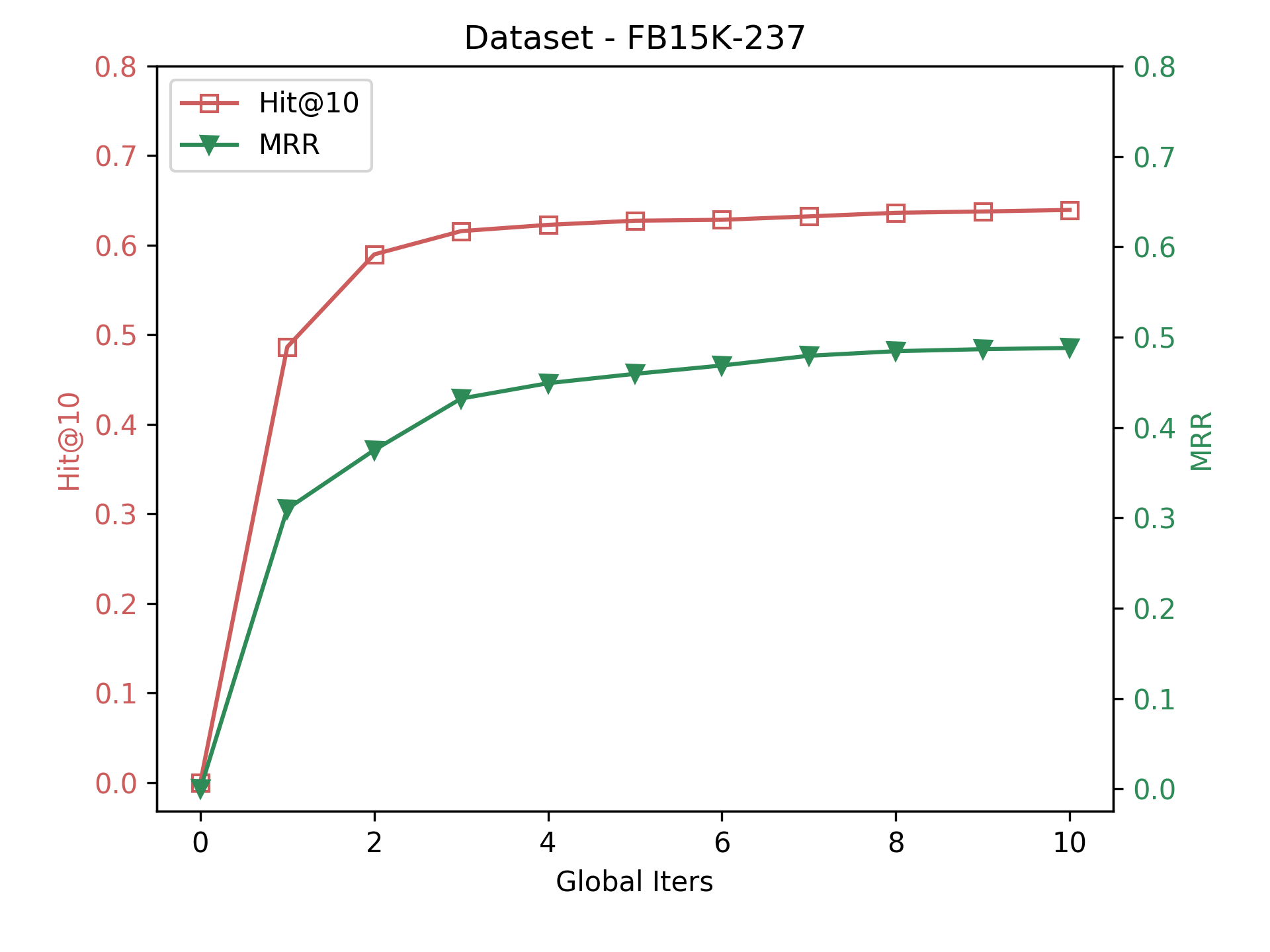
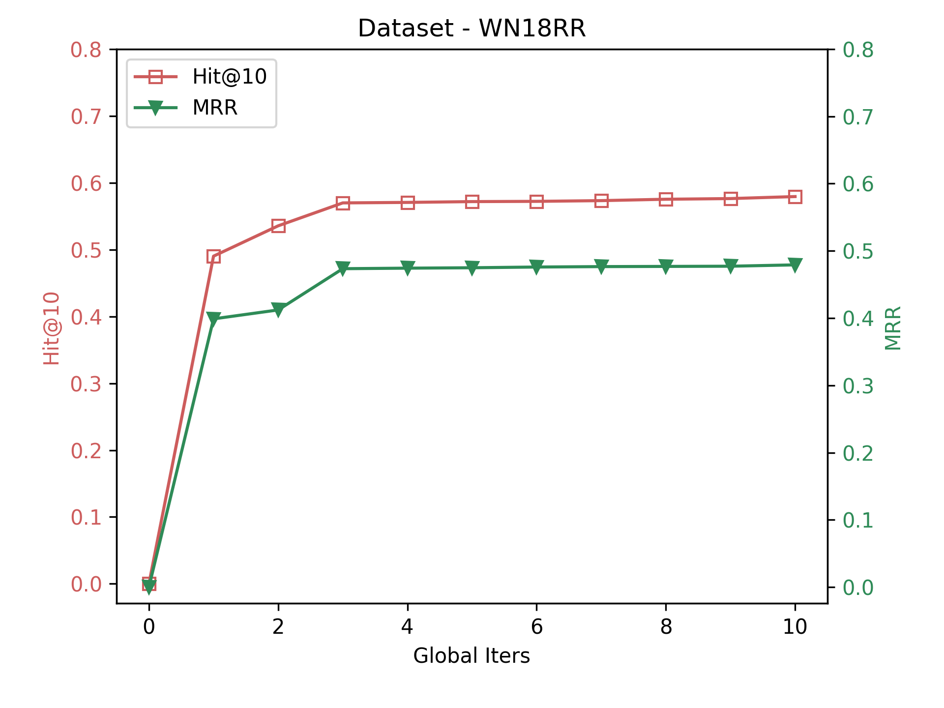
Figure 3: Link Prediction Performance vs Global Iterations

VII-C Case Study

TABLE VII: Qualitative results showing link prediction rank change of entities of test triplets by comparing our method and baseline RotatE. The associated rule used for providing feedback is shown for each test triplet

Test Triplet	(Louis Armstrong, /people/person/nationality, United States)
Rule	/music/artist/origin($V_{0},V_{2}$) $\land$ /location/administrative_division/country($V_{2},V_{1}$) $\rightarrow$ /people/person/nationality($V_{0},V_{1}$)
Rank Change	head: 1154 $\rightarrow$ 68 (+1086) tail: 1 $\rightarrow$ 1 (+0)
Test Triplet	(15 Minutes, /film/country, United States)
Rule	/film/production_companies($V_{0},V_{2}$) $\land$ /organization/headquarters./location/country($V_{2},V_{1}$) $\rightarrow$ /film/country($V_{0},V_{1}$)
Rank Change	head: 314 $\rightarrow$ 12 (+302) tail: 1 $\rightarrow$ 1 (+0)
Test Triplet	(Poland, /location/second_level_divisions, Szczecin )
Rule	/bibs_location/country($V_{2},V_{0}$) $\land$ /location/county_place/($V_{2},V_{1}$)$\rightarrow$ /location/second_level_divisions($V_{0},V_{1}$)
Rank Change	head: 1 $\rightarrow$ 1 (+0) tail: 384 $\rightarrow$ 8 (+376)
Test Triplet	(Fort Lauderdale, /location/location/time_zones, Eastern Time Zone)
Rule	/location/location/contains($V_{0},V_{2}$) $\land$ /location/location/time_zones($V_{2},V_{1}$) $\rightarrow$ /location/location/time_zones($V_{0},V_{1}$)
Rank Change	head: 414 $\rightarrow$ 45 (+369) tail: 1 $\rightarrow$ 1 (+0)

We give some qualitative examples from FB15K-237 dataset to demonstrate the effectiveness of our model. First, consider Table VII. It shows multiple test triplets from $G_{test}$ and their corresponding head and tail rank change when comparing RotatE [8] as baseline with our method. The relevant rule that provides feedback to embedding learning in our framework is also shown for each test triplet. As an example, take the first test triplet (Louis Armstrong, /people/person/nationality, United States). Because Louis Armstrong is a sparse entity with sparsity 0.995, traditional embedding methods suffer in the head prediction task i.e. asking (?, /people/person/nationality, United States) essentially because the embedding representations of sparse entities are not informative. Concretely, RotatE gives a filtered rank of 1154. Compare this to our method which utilizes the rule that says musicians have the same nationality as the country of the town they are originally from. Having $V_{2}$ as New Orleans satisfies the rule for the test triplet and our method improves the subject prediction rank to 68, a gain of 1086. An observation about the tail prediction task, i.e. (Louis Armstrong, /people/person/nationality, ?) conveys that baseline methods perform well when entities are not so sparse for e.g. here it is United States that is not sparse. The other examples show a similar qualitative trend demonstrating that using feedback from relevant rules improves embedding representations of entities especially sparse ones.

TABLE VIII: Qualitative results showing the comparison between standard embeddding confidence scores for three candidate rules inferring the same head atom.

	Rule	Rule Support	No. Predictions	Standard Confidence	Embedding Confidence
1	/olmpic_sport./affiliation_country($V_{0},V_{2}$) $\land$ /location/import_and_exports($V_{2},V_{1}$) $\rightarrow$ /olympic_sport./affiliation_country($V_{0},V_{1}$)	548	1723	0.318	0.207
2	/olympic_sport./affiliation_country($V_{0},V_{2}$) $\land$ /location./adjoins_location($V_{2},V_{1}$) $\rightarrow$ /olympic_sport./affiliation_country($V_{0},V_{1}$)	1524	4747	0.321	0.404
3	/sport./pro_olympic_athlete($V_{0},V_{2}$) $\land$ /person./nationality($V_{2},V_{1}$) $\rightarrow$ /olympic_sport./affiliation_country($V_{0},V_{1}$)	588	1792	0.328	0.701

TABLE IX: TransE with different negative sampling techniques.

	FB15K-237		WN18RR
	MRR	Hit@10	MRR	Hit@10
uniform	0.241	0.422	0.186	0.459
KBGAN	0.278	0.453	0.210	0.479
self-adversarial	0.298	0.475	0.223	0.510
uniform + our method	0.435	0.545	0.234	0.515

Next we show qualitatively how rule quality can be improved with embedding guidance through our embedding confidence measure (Eq. 6). Table VIII shows three different rule bodies mined by AIME+ on FB15K-237, which all result in the same head atom i.e. /olympic_sport./affiliation_country($V_{0},V_{1}$) which means $V_{0}$ is an olympic sport that has representation for country $V_{1}$. An example triplet in $G_{train}$ is (Trialathon, /olympic_sport/affiliation_country, France). Rules one and two say that an olympic sport $V_{0}$ has representation from country $V_{1}$ if there is another country $V_{2}$ that represents $V_{0}$ and is adjoining $V_{1}$ or does trade with it. Both rules get very similar standard confidence measures because the ratio of corresponding rule support and number of predictions is alike and choosing a relevant rule is not clear. Compare this with rule three, which says an olympic sport $V_{0}$ has representation from country $V_{1}$ if there is a professional olympic athlete $V_{2}$ who plays $V_{0}$ and $V_{2}$ has nationality $V_{1}$. This rule is more apt compared to the earlier ones but still gets similar standard confidence of 0.328. Now contrast this with the embedding confidence scores for each of the three rules. Rule three gets a much better EC score compared to one and two because most of its instantiations give high embedding scores (see Eq. 6). This shows that embedding confidence which is able model the rules probabilistically is helpful when used in conjunction with standard confidence to assess the quality of rules when mining.

VII-D Connections to Negative Sampling

The results from the previous section made us look at our paradigm through the lens of negative sampling for explanation. At each iteration, when new inferred triplets are introduced, the underlying uniform negative sampling generates higher quality negatives simply because of the superior positives that are augmented. We further show (Table IX) how our method stacks up against other negative sampling methods like uniform, KBGAN [34] and self-adversarial [8]. For all methods including ours, TransE [6] is used as the embedding method for a fair comparison. The results indicate that the augmented inferred triplets invariably lead to better quality negatives thus improving the overall train set on which the embeddings are learned. In our opinion, this is also a possible explanation for the significant boost in performance for models like TransE and ComplEx that are actually incapable of modelling symmetry and composition patterns in data [8].

VIII Conclusion

In this work, we have developed a hybrid method which utilizes the complementary properties of rules and embeddings. Experimental results empirically support the two main claims we raised (1) structure and richer data quality in training results in superior embedding representations, and (2) incorporation of “global” KG statistical patterns in rule mining lead to reliable rules. We extensively evaluated our approach with varied experiments and showed its effectiveness. The connections to negative sampling motivate us investigate more deeply about the framework in future for possible theoretical claims and develop other general hybrid models for unifying different learning schemes.

References

- [1] Freebase, Freebase Data Dumps, (accessed June 5, 2020). [Online]. Available: https://developers.google.com/freebase/
- [2] F. M. Suchanek, G. Kasneci, and G. Weikum, “Yago: a core of semantic knowledge,” in Proceedings of the 16th international conference on World Wide Web, 2007, pp. 697–706.
- [3] Wikidata, Main page, (accessed June 5, 2020). [Online]. Available: https://www.wikidata.org/
- [4] Google, Google Knowledge Graph, (accessed June 5, 2020). [Online]. Available: https://www.blog.google/products/search/introducing-knowledge-graph-things-not/
- [5] M. Nickel, V. Tresp, and H.-P. Kriegel, “A three-way model for collective learning on multi-relational data.” 2011.
- [6] A. Bordes, N. Usunier, A. Garcia-Duran, J. Weston, and O. Yakhnenko, “Translating embeddings for modeling multi-relational data,” in Advances in neural information processing systems, 2013, pp. 2787–2795.
- [7] T. Trouillon, J. Welbl, S. Riedel, É. Gaussier, and G. Bouchard, “Complex embeddings for simple link prediction,” in International Conference on Machine Learning, 2016, pp. 2071–2080.
- [8] Z. Sun, Z.-H. Deng, J.-Y. Nie, and J. Tang, “Rotate: Knowledge graph embedding by relational rotation in complex space,” arXiv preprint arXiv:1902.10197, 2019.
- [9] B. Goethals and J. Van den Bussche, “Relational association rules: getting w armer,” in Pattern Detection and Discovery. Springer, 2002, pp. 125–139.
- [10] L. Galárraga, C. Teflioudi, K. Hose, and F. M. Suchanek, “Fast rule mining in ontological knowledge bases with amie+,” The VLDB Journal—The International Journal on Very Large Data Bases, vol. 24, no. 6, pp. 707–730, 2015.
- [11] R. Jenatton, N. L. Roux, A. Bordes, and G. R. Obozinski, “A latent factor model for highly multi-relational data,” in Advances in Neural Information Processing Systems, 2012, pp. 3167–3175.
- [12] J. Pujara, E. Augustine, and L. Getoor, “Sparsity and noise: Where knowledge graph embeddings fall short,” in Proceedings of the 2017 Conference on Empirical Methods in Natural Language Processing, 2017, pp. 1751–1756.
- [13] W. Zhang, B. Paudel, L. Wang, J. Chen, H. Zhu, W. Zhang, A. Bernstein, and H. Chen, “Iteratively learning embeddings and rules for knowledge graph reasoning,” in The World Wide Web Conference. ACM, 2019, pp. 2366–2377.
- [14] L. A. Galárraga, C. Teflioudi, K. Hose, and F. Suchanek, “Amie: association rule mining under incomplete evidence in ontological knowledge bases,” in Proceedings of the 22nd international conference on World Wide Web. ACM, 2013, pp. 413–422.
- [15] B. Yang, W.-t. Yih, X. He, J. Gao, and L. Deng, “Embedding entities and relations for learning and inference in knowledge bases,” arXiv preprint arXiv:1412.6575, 2014.
- [16] T. Dettmers, P. Minervini, P. Stenetorp, and S. Riedel, “Convolutional 2d knowledge graph embeddings,” in Thirty-Second AAAI Conference on Artificial Intelligence, 2018.
- [17] M. Nickel, K. Murphy, V. Tresp, and E. Gabrilovich, “A review of relational machine learning for knowledge graphs,” Proceedings of the IEEE, vol. 104, no. 1, pp. 11–33, 2015.
- [18] Q. Wang, Z. Mao, B. Wang, and L. Guo, “Knowledge graph embedding: A survey of approaches and applications,” IEEE Transactions on Knowledge and Data Engineering, vol. 29, no. 12, pp. 2724–2743, 2017.
- [19] S. Muggleton and L. De Raedt, “Inductive logic programming: Theory and methods,” The Journal of Logic Programming, vol. 19, pp. 629–679, 1994.
- [20] R. Agrawal, T. Imieliński, and A. Swami, “Mining association rules between sets of items in large databases,” in Acm sigmod record, vol. 22, no. 2. ACM, 1993, pp. 207–216.
- [21] H. Adé, L. De Raedt, and M. Bruynooghe, “Declarative bias for specific-to-general ilp systems,” Machine Learning, vol. 20, no. 1-2, pp. 119–154, 1995.
- [22] L. Dehaspe and H. Toivonen, “Discovery of relational association rules,” in Relational data mining. Springer, 2001, pp. 189–212.
- [23] R. Agrawal, H. Mannila, R. Srikant, H. Toivonen, and A. I. Verkamo, “Fast discovery of association rules,” in Advances in knowledge discovery and data mining. American Association for Artificial Intelligence, 1996, pp. 307–328.
- [24] S. Schoenmackers, O. Etzioni, D. S. Weld, and J. Davis, “Learning first-order horn clauses from web text,” in Proceedings of the 2010 Conference on Empirical Methods in Natural Language Processing. Association for Computational Linguistics, 2010, pp. 1088–1098.
- [25] K. Toutanova and D. Chen, “Observed versus latent features for knowledge base and text inference,” in Proceedings of the 3rd Workshop on Continuous Vector Space Models and their Compositionality, 2015, pp. 57–66.
- [26] Q. Wang, B. Wang, and L. Guo, “Knowledge base completion using embeddings and rules,” in Twenty-Fourth International Joint Conference on Artificial Intelligence, 2015.
- [27] T. Rocktäschel, S. Singh, and S. Riedel, “Injecting logical background knowledge into embeddings for relation extraction,” in Proceedings of the 2015 Conference of the North American Chapter of the Association for Computational Linguistics: Human Language Technologies, 2015, pp. 1119–1129.
- [28] S. Guo, Q. Wang, L. Wang, B. Wang, and L. Guo, “Knowledge graph embedding with iterative guidance from soft rules,” in Thirty-Second AAAI Conference on Artificial Intelligence, 2018.
- [29] B. Ding, Q. Wang, B. Wang, and L. Guo, “Improving knowledge graph embedding using simple constraints,” arXiv preprint arXiv:1805.02408, 2018.
- [30] B. Fatemi, P. Taslakian, D. Vazquez, and D. Poole, “Knowledge hypergraphs: Extending knowledge graphs beyond binary relations,” arXiv preprint arXiv:1906.00137, 2019.
- [31] F. Mahdisoltani, J. Biega, and F. M. Suchanek, “Yago3: A knowledge base from multilingual wikipedias,” 2015.
- [32] Z. Sun, S. Vashishth, S. Sanyal, P. Talukdar, and Y. Yang, “A re-evaluation of knowledge graph completion methods,” arXiv preprint arXiv:1911.03903, 2019.
- [33] M. Qu and J. Tang, “Probabilistic logic neural networks for reasoning,” in Advances in Neural Information Processing Systems, 2019, pp. 7710–7720.
- [34] L. Cai and W. Y. Wang, “Kbgan: Adversarial learning for knowledge graph embeddings,” arXiv preprint arXiv:1711.04071, 2017.