Quasinormal modes of dirty black holes in the two-loop renormalizable effective gravity.

Abstract

We consider gravitational quasinormal modes of the static and spherically-symmetric dirty black holes in the effective theory of gravity which is renormalizable at the two-loop level. It is demonstrated that using the WKB-Padé summation proposed in Matyjasek and Opala (2017) one can achieve sufficient accuracy to calculate corrections to the complex frequencies of the quasinormal modes caused by the Goroff-Sagnotti curvature terms. It is shown that the Goroff-Sagnotti correction (with our choice of the sign of the coupling constant) increases damping of the fundamental modes (except for the lowest fundamental mode) and decreases their frequencies. We argue that the methods adopted in this paper can be used in the analysis of the influence of the higher-order curvature terms upon the quasinormal modes and in a number of related problems that require high accuracy.

I Introduction

The reaction of a black hole to small perturbations is described by a set of oscillations, called quasinormal, and characterized by complex numbers, $\omega,$ the real part of which gives the frequency of the mode whereas the imaginary part controls its damping rate. Mathematically, the quasinormal modes considered in this paper are the solutions to the ordinary second order Schrödinger-like differential equation

$$\frac{d^{2}}{dx^{2}}\Psi+\left(\omega^{2}-V[r(x)]\right)\Psi=0$$ (1)

with the boundary conditions corresponding to purely outgoing waves at infinity and purely ingoing waves at the horizon. Here $x$ is the tortoise coordinate, $\Psi=\Psi[r(x)]$ describes the radial perturbations in the linear regime and $V$ is the potential. The potential is constant as $|x|\to\infty$ and has a maximum at $x_{0}.$ For the mode of a given spin weight, $j,$ the quasinormal frequencies are labeled by the multipole number, $\ell,$ and the overtone number $n.$

Unfortunately, in the black hole context, it is impossible to solve this equation exactly and consequently one has to resort to numerical and/or approximate methods. Since their discovery by Vishveshwara in 1970 Vishveshwara (1970) an enormous amount of work has been carried out on the quasinormal oscillations. Interested readers are referred to the excellent reviews Kokkotas and Schmidt (1999); Nollert (1999); Konoplya and Zhidenko (2011); Berti et al. (2009) covering almost all aspects of the problem. Here we mention only the most popular and highly accurate numerical approaches: the method of continued fractions Leaver (1985); Nollert (1993); Rostworowski (2007), the Hill determinant method Majumdar and Panchapakesan (1989), asymptotic iteration Cho et al. (2010), the pseudospectral method Jansen (2017) and the method of Nollert and Schmidt Nollert and Schmidt (1992). On the other hand, we have a group of analytic and semi-analytic methods based on the WKB expansion and its variants Schutz and Will (1985); Iyer and Will (1987); Iyer (1987); Kokkotas and Schutz (1988); Seidel and Iyer (1990); Froeman et al. (1992); Andersson and Linneaus (1992); Konoplya (2003) and the related method of Gal’tsov and Matukhin Gal’tsov and Matiukhin (1992). Among the WKB-based approximations the most popular are the (third-order) Iyer-Will method Iyer and Will (1987) and its sixth-order generalization constructed by Konoplya Konoplya (2003). Moreover, coputationally still very promising is the method developed by Zaslavskii Zaslavskii (1991), who following the ideas of Refs. Blome and Mashhoon (1984); Ferrari and Mashhoon (1984a, b) reduced the problem to the calculation of the energy levels of the quantum anharmonic oscillator. As has been demonstrated in Ref. Zaslavskii (1991), one can reproduce the Iyer-Will Iyer and Will (1987) results by calculating the first two nontrivial corrections to the energy levels of the sixth-order anharmonic oscillator and this equivalence can be extended to higher orders Matyjasek and Telecka (2019).

Recently, it has been proposed to construct the Padé transform of the WKB series describing complex frequencies of the quasinormal modes instead of just summing them term by term Matyjasek and Opala (2017); Matyjasek and Telecka (2019). This approach appears to be a major improvement over the pure WKB method. Indeed, its has been shown in Refs Matyjasek and Opala (2017); Matyjasek and Telecka (2019) that (within the domain of applicability) one can obtain highly accurate values of the quasinormal frequencies. Depending on the number of terms retained in the WKB expansion one can achieve the accuracy of (at least) 24 decimal places for the low-lying modes.

The aforementioned techniques have been successfully applied to various black hole systems, too numerous to list them here. Once again the reader is referred to review papers. Here we shall discuss certain aspects of the effective gravity in the context of the quasinormal oscillations of black holes. The influence of the higher-order curvature terms (see, e.g., Refs Myers (1999); Lu and Wise (1993); Matyjasek et al. (2006); Dobado and Maroto (1993) ) on quasinormal modes has attracted some attention recently. (See for example Refs. Konoplya et al. (2020); Momennia and Hendi (2020); Bouhmadi-López et al. (2020) and the references cited therein). In this paper we shall investigate this problem in some detail. We will limit ourselves to the two-loop renormalizable effective gravity and concentrate on the following issues: First, we check if the adapted method (which is based on the results of Refs. Matyjasek and Opala (2017); Matyjasek and Telecka (2019)) is sufficiently sensitive to quantify the influence of the higher order terms upon the quasinormal modes. Secondly, we compare the complex frequencies calculated for the classical black hole and its two-loop counterpart. Finally, we will briefly discuss the danger of relying too much on the schemes that involve only a few first terms of the WKB expansion.

The paper is organized as follows. In Sec. II we study the spherically-symmetric black holes in the two-loop renormalizable effective gravity and give main equations of the problem. In Sec. III.1 we illustrate the adopted method using simple Mashhoon Mashhoon and Schutz-Will Schutz and Will (1985) approach with the Regge-Wheeler and the Zerilli potentials expressed in terms of the Lambert functions. The corrections caused by the sixth-order terms are presented graphically. The accurate calculations of the quasinormal modes are carried out in Sec. III.2, where we also study the influence of the second-order corrections to the black hole solution on the quasinormal frequencies. Finally, in Sec. IV we discuss the results obtained and the dangers of naive summation of the WKB terms or using simplistic methods.

Throughout the paper we use natural units $c=G=1.$ The signature of the metric is taken to be “mainly positive”, i.e., $+2,$ and the conventions for the curvature tensor are $\mathcal{R}^{a}_{\,bcd}=\partial_{c}\Gamma^{a}_{\,bd}...,$ and $\mathcal{R}^{a}_{\,bac}=\mathcal{R}_{bd}$.

II Dirty black holes

As is well-known, the macroscopic black holes are sensitive to the higher-order terms in the gravitational action. Typically, such terms are constructed from the basis of the curvature monomial invariants of definite order and degree and appear in a natural way in the low-energy limit of the string theory, phenomenological effecitve Lagrangians and the Lovelock gravity. Moreover, the renormalized one-loop effective action of the quantized massive fields in the large mass limit is constructed form the curvature invariants (the type of the field enters through the spin-dependent numerical coefficients). The general gravitational action of this type can be written as

$$S_{g}=\sum_{k=0}^{m}\alpha_{k}S_{k},$$ (2)

where each $S_{k}$ is constructed from the curvature invariants of the definite order $s$ (the number of differentiations of the metric) and degree $q$ (the number of factors). Here $s=2k,$ $S_{0}$ is related to the cosmological term and $S_{1}$ is the standard Einstein-Hilbert action. The total action is therefore the sum of the gravitational action and the matter contribution, where the latter may also contain quantum corrections. The result of the functional differentiations of the total action with respect to the metric tensor can generally be written as

$$\mathcal{R}_{ab}-\frac{1}{2}\mathcal{R}g_{ab}+\Lambda g_{ab}+\mathcal{P}_{ab}=8\pi\left(T_{ab}+T_{ab}^{(1)}\right),$$ (3)

where $\mathcal{P}_{ab}$ represents the result of the functional differentiation of the higher-order curvature terms, $T_{ab}$ is the stress-energy tensor of the classical matter, $T_{ab}^{(1)}$ is a small correction (presumably of quantum origin) and all the remaining symbols have their usual meaning. Both the left and the right hand side of (3) functionally depends on the metric tensor. Of course, there is no necessity to introduce $P_{ab}$ and $T_{ab}^{(1)}$ terms simultaneously, typically we have either one or the other present. It should be noted that when the tensor $T_{ab}^{(1)}$ is of purely geometric origin it may (with some reservations), equally well, be treated as the object that modifies the left hand side of the equations Matyjasek (2001, 2004).

One of the most important and interesting applications of the higher-order theories of gravitation is the search for their imprints on classical configurations modeled by the solutions of the Einstein field equations. This should lead to some definite predictions. Unfortunately, the complexity of the problem practically excludes construction of the exact solutions and one is forced to adopt either some approximations or refer to numerics. Here we shall choose the first option. To illustrate the procedure, we consider the simplest case of the spacetime generated by the spherically symmetric matter distribution. The line element describing the spacetime in question can be written as

$$ds^{2}=-e^{-2\psi}\left(1-\frac{2m}{r}\right)dt^{2}+\left(1-\frac{2m}{r}\right)^{-1}dr^{2}+r^{2}d\Omega^{2},$$ (4)

where $m=m(r)$ and $\psi=\psi(r)$ are two functions of the radial coordinate and $d\Omega^{2}$ denotes the metric on the unit sphere. The functions $m(r)$ and $\psi(r)$ are model-dependent, i.e., they are the solutions of the Einstein field equations describing the particular model. Now, let us assume that the line element (4) describes a black hole with the event horizon located at $r=r_{+}.$ In what follows we shall refer to this configuration as ‘dirty’ or ‘corrected’ black hole. For the line element (4) the field equations (3) with the cosmological constant set to zero assume the form

$$-\frac{2}{r^{2}}\frac{dm}{dr}+\varepsilon P_{t}^{t}=8\pi\left(T_{t}^{t}+\varepsilon T_{t}^{(1)t}\right)$$ (5)

and

$$-\frac{2}{r^{2}}\frac{dm}{dr}-\frac{2}{r}\frac{d\psi}{dr}\left(1-\frac{2m(r)}{r}\right)+\varepsilon P_{r}^{r}=8\pi\left(T_{r}^{r}+\varepsilon T_{r}^{(1)r}\right),$$ (6)

where $\varepsilon$ is the dimensionless parameter that helps to keep track of the order of terms in complicated expansions, and as such, it should be set to 1 at the end of the calculation.

The potential of the gravitational perturbations can be written in the form Medved et al. (2004a, b)

$$V(r)=e^{-2\psi}\left(1-\frac{2m}{r}\right)\left[\frac{\ell(\ell+1)}{r^{2}}-\frac{6m}{r^{3}}+\frac{2}{r^{2}}\frac{dm}{dr}+\frac{1}{r}\left(1-\frac{2m}{r}\right)\frac{d\psi}{dr}\,\right].$$ (7)

With $m(r)=\mathcal{M}$ and $\psi(r)=0$ the potential $V(r)$ reduces to the Regge-Wheeler potential of the Schwarzschild black hole. It belongs to a more general class of potentials describing scalar, vector and gravitational perturbations

$$V(r)=e^{-2\psi}\left(1-\frac{2m}{r}\right)\left[\frac{\ell(\ell+1)}{r^{2}}+(1-j^{2})\frac{2m}{r^{3}}-(1-j)\,\mathcal{R}_{\theta}^{\theta}\,\right],$$ (8)

where

$$j=\begin{cases}0&{\rm for\,scalar}\\ 1&{\rm for\,vector}\\ 2&{\rm for\,gravity}\end{cases}$$ (9)

and the angular components of the Ricci tensor are given by

$$\mathcal{R}_{\theta}^{\theta}=\mathcal{R}_{\phi}^{\phi}=\frac{2}{r^{2}}\frac{dm}{dr}+\frac{1}{r}\left(1-\frac{2m}{r}\right)\frac{d\psi}{dr}.$$ (10)

Our discussion has been exact up to this point. Now, let us assume that the functions $m(r)$ and $\psi(r)$ have the following expansion

$$m(r)=\sum_{k=0}^{N}\varepsilon^{k}M_{k}(r)+\mathcal{O}(\varepsilon^{N+1})$$ (11)

and

$$\psi(r)=\sum_{k=1}^{N}\varepsilon^{k}\psi_{k}(r)+\mathcal{O}(\varepsilon^{N+1}),$$ (12)

where $\varepsilon$ is the dimensionless parameter. Note that the term $\psi_{0}$ has no independent physical meaning and is omitted. The system of the differential equations has to be supplemented with the suitable boundary conditions. In what follows we shall relate the additive integration constant with the total mass of the system measured from infinity $r_{\infty},$ i.e., $m(r_{\infty})=\mathcal{M},$ whereas the second integration constant can be determined from the natural condition $\psi(r_{\infty})=0.$ Now, inserting the expansions of the functions $m(r)$ and $\psi(r)$ into Eqs. (5) and (6) and collecting terms with like powers of $\varepsilon,$ one obtains a system of the ordinary differential equations of ascending complexity.

Let us concentrate on pure gravity. As is well known, the one-loop corrections to the pure classical gravity are quadratic and the divergent terms calculated by ’t Hooft and Veltman have the form ’t Hooft and Veltman (1974)

$$\frac{1}{(4\pi)^{2}(D-4)}\left(\frac{1}{120}\mathcal{R}_{ab}\mathcal{R}^{ab}+\frac{7}{20}\mathcal{R}^{2}\right),$$ (13)

where $D$ is the dimension. Hence the one-loop divergences of pure gravity vanish on-shell, the result that can be obtained on the basis of symmetry. In their seminal papers, Goroff and Sagnotti Goroff and Sagnotti (1985, 1986) showed that at the two-loop level the divergences of the gravitational action are encoded in the term

$$\frac{209}{2880(4\pi)^{2}(D-4)}\int d^{4}x\,\sqrt{-g}\,\mathcal{R}_{ab}^{\phantom{c}\phantom{d}cd}\mathcal{R}_{cd}^{\phantom{c}\phantom{d}ef}\mathcal{R}_{ef}^{\phantom{c}\phantom{d}ab},$$ (14)

and thus the Einstein theory of gravitation is not renormalizable. Although this result seems to be quite pessimistic, one can think of it as the indication of possible modifications of the Einstein gravity. Indeed, introducing the term proportional to

$$S_{3}=\int d^{4}x\,\sqrt{-g}\,\mathcal{R}_{ab}^{\phantom{c}\phantom{d}cd}\mathcal{R}_{cd}^{\phantom{c}\phantom{d}ef}\mathcal{R}_{ef}^{\phantom{c}\phantom{d}ab}$$ (15)

to the total action one obtains, in concord with the philosophy of the effective lagrangians, a simplest generalization of the pure Einstein gravity that absorbs the divergent term. At the level of the field equations $S_{3}$ introduces the term proportional to

$$\frac{1}{\sqrt{-g}}\frac{\delta}{\delta g_{ab}}S_{3} = -12\mathcal{R}_{c\phantom{b};d}^{\phantom{c}b\phantom{;\phantom{d}}}\mathcal{R}_{\phantom{c}\phantom{a}\phantom{;\phantom{d}}}^{ca;d}+12\mathcal{R}_{c\phantom{b};d}^{\phantom{c}b\phantom{;\phantom{d}}}\mathcal{R}_{\phantom{d}\phantom{a}\phantom{;\phantom{c}}}^{da;c}-6\mathcal{R}_{cde\phantom{b};i}^{\phantom{c}\phantom{d}\phantom{e}b\phantom{;\phantom{i}}}\mathcal{R}_{\phantom{c}\phantom{d}\phantom{i}\phantom{a}\phantom{;\phantom{e}}}^{cdia;e}+12\mathcal{R}_{c\phantom{b};de}^{\phantom{c}b\phantom{;\phantom{d}}\phantom{e}}\mathcal{R}_{\phantom{c}\phantom{d}\phantom{e}\phantom{a}}^{cdea}\mathcal{R}$$

$$+12\mathcal{R}_{c\phantom{a};de}^{\phantom{c}a\phantom{;\phantom{d}}\phantom{e}}\mathcal{R}_{\phantom{c}\phantom{d}\phantom{e}\phantom{b}}^{cdeb}-12\mathcal{R}_{cdei}^{\phantom{c}\phantom{d}\phantom{e}\phantom{i}}\mathcal{R}_{j\phantom{c}\phantom{e}\phantom{b}}^{\phantom{j}ceb}\mathcal{R}_{\phantom{d}\phantom{j}\phantom{i}\phantom{a}}^{djia}-6\mathcal{R}_{cd}^{\phantom{c}\phantom{d}}\mathcal{R}_{ei\phantom{c}\phantom{b}}^{\phantom{e}\phantom{i}cb}\mathcal{R}_{\phantom{d}\phantom{a}\phantom{e}\phantom{i}}^{daei}+\frac{1}{2}g_{\phantom{a}\phantom{b}}^{ab}\mathcal{R}_{cdei}^{\phantom{c}\phantom{d}\phantom{e}\phantom{i}}\mathcal{R}_{jk\phantom{c}\phantom{d}}^{\phantom{j}\phantom{k}cd}\mathcal{R}_{\phantom{e}\phantom{i}\phantom{j}\phantom{k}}^{eijk}.$$

Now, let us analyze the influence of the higher-derivative terms that may appear in the low-energy effective action functional on the complex frequencies of the quasinormal modes. To keep the calculations as simple as possible we neglect, in concord with our previous discussion, the four derivative terms and restrict ourselves to the first order expansion of the functions $m(r)$ and $\psi(r).$ Additionally we assume that the total stress-energy tensor vanishes and the sixth-order term (15) is the only source of the modifications of the vacuum field equations. The total (effective) action is therefore given by

$$S_{total}=\int d^{4}x\sqrt{-g}\,\mathcal{R}-\alpha\int d^{4}x\,\sqrt{-g}\,\mathcal{R}_{ab}^{\phantom{c}\phantom{d}cd}\mathcal{R}_{cd}^{\phantom{c}\phantom{d}ef}\mathcal{R}_{ef}^{\phantom{c}\phantom{d}ab}.$$ (17)

Our first task is to solve the field equations. To this end, let us return to the spherically symmetric line element (4) with (11) and (12). Now, making a substitution $\alpha\to\varepsilon\alpha$ and subsequently, as has been mentioned earlier, functionally differentiating the total gravitational action with respect to the metric tensor, inserting the line element to the thus obtained system of the differential equations and finally expanding the result in the powers of $\varepsilon,$ one obtains a chain of differential equations for $\psi_{i}(r)$ and $M_{i}(r).$ The zeroth-order solution is the Schwarzschild line element characterized by the mass $\mathcal{M},$ whereas the first order equations can be written as

$$-\frac{2}{r^{2}}\frac{dM_{1}(r)}{dr}+\,{\frac{24\mathcal{M}^{2}\left(98\,{\mathcal{M}}-45\,r\right)}{{r}^{9}}}=0$$ (18)

and

$$-\frac{d\psi_{1}(r)}{dr}+\frac{648\mathcal{M}^{2}}{r^{7}}=0.$$ (19)

They can be easily integrated and the perturbative solution to the sixth-order gravity field equations is given by

$$m(r)=\mathcal{M}-\alpha\frac{4\mathcal{M}^{2}}{r^{6}}\left(49\mathcal{M}-27r\right)$$ (20)

and

$$\psi_{1}(r)=-\alpha\frac{108\mathcal{M}^{2}}{r^{6}},$$ (21)

where $\varepsilon$ has been put to 1. Since the black hole solution is characterized by a total mass as seen by a distant observer, the corrected location of the event horizon is

$$r_{+}=2\mathcal{M}\left(1+\frac{5\alpha}{16\mathcal{M}^{4}}\right).$$ (22)

It should be noted that the solution we just found is equivalent to the solution constructed in Ref. Dobado and Maroto (1993), where $g_{00}$ and $g_{11}$ have been expanded in the powers of $r^{-1}.$ The coefficients of the expansion satisfy a system of algebraic equations. Indeed, inserting (20) and (21) into (4), expanding the result in $\varepsilon$ and finally making substitution $\alpha\to 16\pi\alpha,$ one obtains precisely the solution presented in Dobado and Maroto (1993). We prefer our method simply because it is (in our opinion) more natural and for higher orders it reduces to simple quadratures. More information is given at the end of Sec. III.2.

Of course, the representation given by (20) and (21) is not unique. One can, equally well, make use of the another set of conditions: $m(r_{+})=r_{+}/2$ and $\psi(r_{\infty})=0,$ where $r_{+}$ is the corrected location of the event horizon. In what follows, however, we will use the former parametrization and characterize the black hole by its total mass as seen by a distant observer rather than the radius of the event horizon.

III Quasinormal modes

Let us return to our discussion of the quasinormal modes and observe that the potential $V(r)$ of the gravitational $(j=2)$ perturbations of the black holes described by the line element (4) with (20) and (21) is given by

$$V(r)=\frac{1}{r}\left(1-\frac{2\mathcal{M}}{r}\right)\left(\frac{L}{r}-\frac{6\mathcal{M}}{r^{2}}\right)-\frac{8\mathcal{M}^{2}\alpha}{r^{10}}\left(528\mathcal{M}^{2}-549\mathcal{M}r+5\mathcal{M}Lr+135r^{2}\right),$$ (23)

where $L=\ell(\ell+1).$ Here we focus on the gravitational modes; the scalar and electromagnetic perturbations can be analyzed in a similar manner. It can be easily checked that (23) vanishes at the event horizon, as expected. In what follows we also need the radial coordinate of the maximum of the effective potential. A simple calculation shows that it is given by

$$r_{0}=r_{(0)}+\alpha\,r_{(1)},$$ (24)

where

$$r_{(0)}=\frac{\left(3L+9+\sqrt{9L^{2}-42L+81}\right)\mathcal{M}}{2L},$$ (25)

$$r_{(1)}=-\frac{4\mathcal{M}^{2}\left(3(5L-549)\mathcal{M}r_{(0)}+1760\mathcal{M}^{2}+360r_{(0)}^{2}\right)}{r_{(0)}^{5}\left(40\mathcal{M}^{2}-4(L+3)\mathcal{M}r_{(0)}+Lr_{(0)}^{2}\right)}.$$ (26)

Asymptotically, as $\ell\to\infty,$ the leading behavior of $r_{(0)}$ and $r_{(1)}$ is given, respectively, by

$$r_{(0)}\sim 3\mathcal{M}+\frac{\mathcal{M}}{\ell^{2}}$$ (27)

and

$$r_{(1)}\sim\frac{20}{81\mathcal{M}^{3}}+\frac{356}{729\mathcal{M}^{3}\ell^{2}}.$$ (28)

Now, we have all the necessary ingredients to calculate the complex frequencies of the quasinormal modes.

III.1 The first-order approach

Our strategy for calculating the quasinormal modes can be illustrated by the following simple example, that is, nevertheless, valid for $\ell\gg 1.$ It would be instructive to analyze it in some detail as the more accurate approaches roughly follow a similar path. This (first-order) approach is mainly due to Mashhoon Mashhoon and Schutz and Will Schutz and Will (1985), and it leads to the following simple and elegant expression

$$iQ_{0}/\left(Q_{0}^{\prime\prime}\right)^{1/2}=\left(n+\frac{1}{2}\right),$$ (29)

where $n=0,1,2,..,$ $Q_{0}=\omega^{2}-V_{0}$ and prime denotes differentiation with respect to the tortoise coordinate $x.$ Here, the subscript ‘0’ means that the subscripted quantity has to be evaluated at the maximum of the potential. The relation (29) can be rewritten in the following simple ‘ready to use’ form

$$\omega^{2}=V_{0}-i\left(n+\frac{1}{2}\right)\left(2Q_{0}^{\prime\prime}\right)^{1/2}.$$ (30)

This formula is the starting point for various more profound analyses and is an indispensable tool in determining the order of magnitude and the general behaviour of the modes. Moreover, for more complex potentials (as the one studied here) the MSW method allows splitting of the quasinormal frequencies into two parts: the classical part and the correction, each of which can be calculated and studied independently. It is evident that the methods based on the summation of the higher-order WKB terms also share this property. Unfortunately, even for such simple approximation as that given by (30), the analytic formulas are too complicated (and not very illuminating) to be shown here. Instead, we will present the results of our calculations graphically.

To illustrate the approach we have calculated frequencies of the all fundamental gravitational modes for $2\leq\ell\leq 100.$ The calculated frequencies have the general form

$$\omega=\omega_{0}+\alpha\delta\omega,$$ (31)

where $\omega_{0}$ denotes the frequencies of the classical Schwarzschild black hole, $\delta\omega$ is the correction and $\alpha$ is the coupling constant. It should be noted that the modifications of the results caused by the two-loop gravity effects are expected to be small and consequently in order to detect them very accurate results for both the Schwarzschild and the dirty black hole are needed. Since the formula (30) gives only qualitative information (although it gets progressively better with increasing $\ell$) it cannot be used for the actual comparisons. On the other hand, its simplicity and the fact that for a given potential both $\omega_{0}$ and $\delta\omega$ are the known (although very complicated) functions of the parameters $\ell$ and $n$ makes this approach ideal for preliminary analyses. The results of the calculations are plotted in Figs 1 and 2.

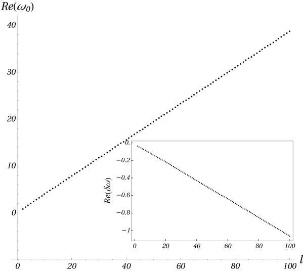
Figure 1: The real part of the quasinormal frequencies of the fundamental modes for $2\leq\ell\leq 100.$ Here $\omega_{0}$ and $\delta\omega$ denote respectively the frequencies of the quasinormal oscillations of the classical black hole and their corrections.

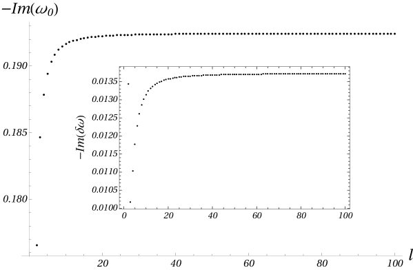
Figure 2: The imaginary part of the quasinormal frequencies of the fundamental modes for $2\leq\ell\leq 100.$ Here $\omega_{0}$ and $\delta\omega$ denote respectively the frequencies of the quasinormal oscillations of the classical black hole and their corrections. The asymptotic value of $\Im(\omega_{0})$ and $\Im(\delta\omega)$ as $\ell\to\infty$ is $-(27)^{-1/2}$ and $-\frac{52}{729}(27)^{-1/2},$ respectively.

Inspection of the figures shows that the behavior of the real and the imaginary part of $\delta\omega$ follows the behavior of the Schwarzschild modes. Indeed, the linear dependence of $\Re(\omega_{0})$ on $\ell$ is also visible in $\Re(\delta\omega).$ For $\alpha>0,$ the sixth-order terms tend to decrease the real part of the frequency. Similarly, the imaginary part of the corrections follows the pattern of $\Im(\omega_{0}),$ making the modes slightly more damped. Finally, observe that both $\Im(\omega_{0})$ and $\Im(\delta\omega)$ asymptotically approach well defined limits. Indeed, $\Im(\omega_{0})=-(27)^{-1/2}=-0.192450$ and $\Im(\delta\omega)=-\frac{52}{729}(27)^{-1/2}=-0.013728$ as $\ell\to\infty.$

Let us return to the Schwarzschild black hole. Inverting standard relation between the radial and the Regge-Wheeler coordinates

$$x=r+2\mathcal{M}\ln\left(\frac{r}{2\mathcal{M}}-1\right)$$ (32)

and expressing the result in term of the principal branch of the Lambert $\mathcal{W}$ function, one has

$$r=2\mathcal{M}\left(1+\mathcal{W}(y)\right),$$ (33)

where $y=\exp(x/(2\mathcal{M})-1).$ Now, the Regge-Wheeler potential can be written in the form

$$V_{0}=\frac{\mathcal{W}(y)\left[\ell(\ell+1)W(y)-3\right]}{4\left(1+\mathcal{W}(y)\right)^{4}},$$ (34)

whereas a slightly more complicated Zerilli potential assumes the form

$$V_{0}=\mathcal{W}(y)\frac{9+18\beta\,[1+\mathcal{W}(y)]+12\beta^{2}\,[1+\mathcal{W}(y)]^{2}+8\beta^{2}(1+\beta)[1+\mathcal{W}(y)]^{3}}{4\,[1+\mathcal{W}(y)]^{4}\,[3+2\beta(1+\mathcal{W}(y)]^{2}},$$ (35)

where $\beta=(l-1)(l+2)/2.$ We prefer this representation over the standard one simply because it depends explicitly on the Regge-Wheeler coordinate $x.$ Now, in order to make use of Eq.(30) it suffices to calculate $x_{0}$ and the second derivative of the potentials with respect to $x$ at $x_{0}.$ Results for the first nine fundamental gravitational modes are tabulated in Table 1. Even a brief analysis of the results shows that the accuracy is not high. Moreover, taking into account a few additional WKB terms does not necessarily improve the quality of the approximation. The foregoing analysis indicates that using simple approximation schemes naively, the calculated corrections may be smaller than the deviations between the approximate and the exact quasinormal frequencies of the classical black hole, so care is needed.

Table 1: The complex frequencies of the fundamental gravitational quasinormal modes of the Schwarzschild black hole calculated for the Regge-Wheeler potential (left column) and the Zerilli potential (right column).

$\ell$	$\omega_{RW}$	$\omega_{Z}$
2	$0.7976992-0.1765708i$	$0.7977882-0.1767022i$
3	$1.2331224-0.1846363i$	$1.2331234-0.1846375i$
4	$1.6446063-0.1878587i$	$1.6446064-0.1878588i$
5	$2.0459245-0.1894270i$	$2.0459245-0.1894270i$
6	$2.4420040-0.1903071i$	$2.4420040-0.1903071i$
7	$2.8350206-0.1908507i$	$2.8350206-0.1908507i$
8	$3.2260873-0.1912102i$	$3.2260873-0.1912102i$
9	$3.6158342-0.1914605i$	$3.6158342-0.1914605i$
10	$4.0046454-0.1916419i$	$4.0046454-0.1916419i$

A very important lesson that follows from this analysis is the observation that, in principle, it should be possible to differentiate between the ‘ideal’ and the dirty black holes, even if the corrections caused by the external factors are small. To do so, however, it is necessary to have a reliable, robust and accurate method for calculation the complex frequencies. Moreover, in view of the expected smallness of the corrections the adopted techniques should allow to work with as many decimal places as needed.

III.2 Padé approximants

Before we extend the above analysis and make our calculations much more accurate let us discuss the options we have. First, it would be natural to extend the method of calculations along the lines developed by Iyer and Will Iyer and Will (1987). As has been demonstrated in Refs. Iyer and Will (1987); Iyer (1987); Kokkotas and Schutz (1988); Konoplya (2003); Matyjasek and Opala (2017) it usually gives slightly more accurate results than its simplified version given by Schutz and Will (1985). The formula relating the complex frequencies of the quasinormal modes and the derivatives of $Q(x)$ at $x=x_{0}$ can be written in the form

$$\frac{iQ_{0}}{\sqrt{2Q^{\prime\prime}_{0}}\tilde{\varepsilon}}-\sum_{k=2}^{N}\tilde{\varepsilon}^{k-1}\Lambda_{k}=n+\frac{1}{2},$$ (36)

where the overtones are labeled by $n$ and $\tilde{\varepsilon}$ is the expansion parameter that helps to keep track of the order of terms in the expansion. The parameter $\tilde{\varepsilon}$ must not be confused with $\varepsilon.$ Each $\Lambda_{k}$ is a combination of the derivatives of $Q(x)$ calculated at $x_{0}$ and its complexity grows fast with the order. The general form of the functions $\Lambda_{k}$ are known for $k\leq 16$ and, in principle, it is possible to construct the analog of Eq.(31). However, since the Iyer-Will technique consists of just summing up the $\Lambda$ terms it cannot be used to obtain highly accurate results. Moreover, increasing the number of $\Lambda$ terms does not improve the quality of the approximation. On the contrary, it can be shown that the moduli of the real and imaginary parts of the quasinormal frequencies rapidly grow with the number of the terms of WKB series summed.

A second approach, and the one that will be used here, consists of treating the right hand side of the expression

$$\omega^{2}=V(x_{0})-i\left(n+\frac{1}{2}\right)\sqrt{2Q^{\prime\prime}_{0}}\tilde{\varepsilon}-i\sqrt{2Q^{\prime\prime}_{0}}\sum_{i=2}^{N}\tilde{\varepsilon}^{j}\Lambda_{j}\equiv V(x_{0})+\sum_{i=1}^{N}\tilde{\varepsilon}^{i}\tilde{\Lambda}_{i}$$ (37)

as the power series and instead of summing the terms (which is a bad strategy) we construct the Padé approximants Matyjasek and Opala (2017); Matyjasek and Telecka (2019). The Padé approximants of a formal power series $\sum a_{k}\tilde{\varepsilon}^{k}$ are defined as the unique rational functions $\mathcal{P}_{N}^{M}(\tilde{\varepsilon})$ of degree $N$ in the denominator and $M$ in the numerator satisfying Bender and Orszag (1978)

$$\mathcal{P}_{N}^{M}(\tilde{\varepsilon})-\sum_{k=0}^{M+N}a_{k}\tilde{\varepsilon}^{k}={\cal{O}}(\tilde{\varepsilon}^{M+N+1}).$$ (38)

It has been shown that this simple strategy yields amazingly accurate results. For example, it can be demonstrated that for the low-lying fundamental gravitational modes of the Schwarzschild black hole one can easily achieve accuracy of 32 decimal places or better. Such accuracy is a must as we are interested in the corrections to $\omega_{0}$ caused by the very subtle effects. The Padé summation of the WKB terms in Eq.(37) has been introduced in Ref. Matyjasek and Opala (2017) and subsequently extended in Ref.Matyjasek and Telecka (2019) to which the interested reader is referred for the technical details and a general discussion. Although the functions $\Lambda_{k}$ for $k\geq 17$ are unknown, they can be constructed for a given potential with prescribed $\ell$ and $n$ numerically Matyjasek and Telecka (2019); Hatsuda (2020b); Sulejmanpasic and Ünsal (2018). Since the approach is numerical it is practically impossible to construct the complex frequencies of the quasinormal modes for a general coupling constant. On the other hand, the calculations can be repeated as many times as needed with various choices of the coupling constant $\alpha,$ and, consequently, given the expected benefits, the loss of the analyticity in the coupling constant can be treated as a minor sacrifice.

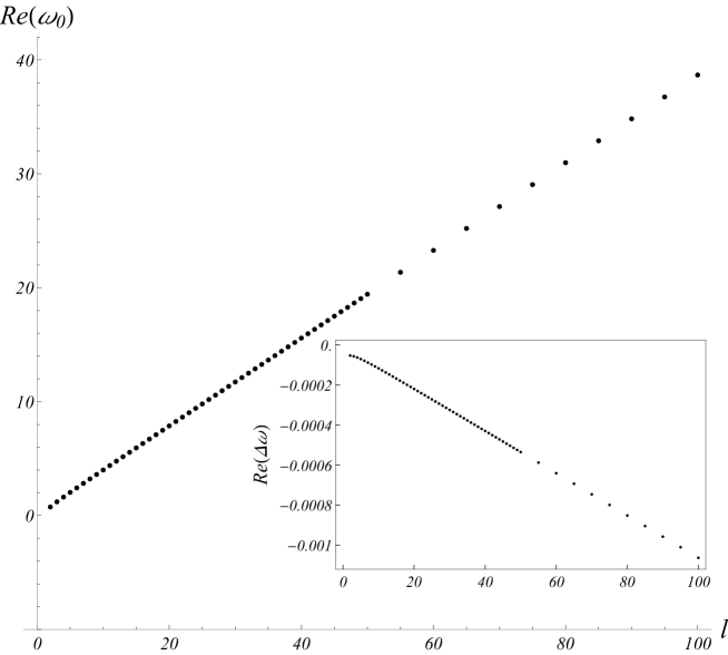
Figure 3: The real part of the quasinormal frequencies of the fundamental modes for $2\leq\ell\leq 100$ calculated for $\alpha=10^{-3}.$ Here $\omega_{0}$ and $\Delta\omega$ denote respectively the frequencies of the quasinormal oscillations of the classical black hole and their corrections. As the quality of the approximation grows with $\ell,$ starting with $\ell=50$ we reduced the number of calculated modes.

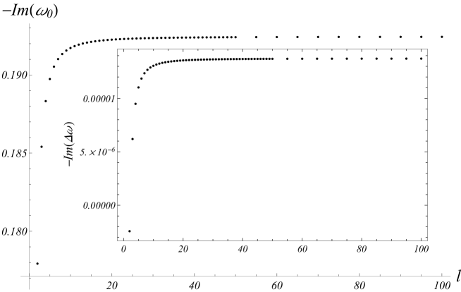
Figure 4: The imaginary part of the quasinormal frequencies of the fundamental modes for $2\leq\ell\leq 100$ calculated for $\alpha=10^{-3}.$ Here $\omega_{0}$ and $\Delta\omega$ denote respectively the frequencies of the quasinormal oscillations of the classical black hole and their corrections. As the quality of the approximation grows with $\ell,$ starting with $\ell=50$ we reduced the number of calculated modes.

Since we do not know the coupling parameter $\alpha$ and the adopted method requires knowledge of its numerical value, we shall consider a toy model in which $\alpha=10^{-3}.$ Such a choice, although unphysical, guarantees that the corrections will be easily visible in the final results. Of course the method is capable of a very high precision and allows for much smaller values of $\alpha$ as will be demonstrated explicitly at the end of this section.

Because of the nature of the problem at hand we want to (numerically) construct the quantities $\omega$ and $\Delta\omega(\alpha)$ that satisfy

$$\omega=\omega_{0}+\Delta\omega(\alpha)$$ (39)

and $\Delta\omega(\alpha)\to 0$ as $\alpha\to 0.$ Before we start the presentation of the results let us briefly discuss the general features of the method. First, it should be observed that for a given $N,$ the accuracy of the Padé transform $\mathcal{P}_{N}^{N}$ increases with $\ell$ and decreases with $n.$ On the other hand, increasing of $N$ improves the accuracy of the overtones. Of course, for each problem there is a minimal $N$ starting with which one obtains sensible results. Since we are interested in a moderate accuracy of the fundamental gravitational quasinormal modes, say up tp 20 decimal places, it suffices to start with $\mathcal{P}_{150}^{150}$ and gradually decrease $N$ with increasing $\ell.$ For example, it suffices to take $N=40$ for $\ell=10.$ Unfortunately, for more complex potentials this places severe demands on the computer resources.

Table 2: The complex frequencies of the fundamental gravitational quasinormal modes of the Schwarzschild black hole (left column) and the dirty black hole (right column) calculated for $\alpha=10^{-3}.$ The Padé approximants of the WKB series, $\mathcal{P}_{N}^{N},$ are calculated for $N=150.$

$\ell$	$\omega_{0}$	$\omega$
2	$0.747343368836083672-0.177924631377871397i$	$0.747289996857394327-0.177922202116315106i$
3	$1.198886576874980146-0.185406095889895208i$	$1.198829745091059250-0.185412294358677386i$
4	$1.618356755064478281-0.188327921977846499i$	$1.618293764592806149-0.188337413836831943i$
5	$2.024590624270701002-0.189741032163219024i$	$2.024519942903865805-0.189752057406537987i$
6	$2.424019641304260981-0.190531691684164105i$	$2.423940385532620070-0.190543545087114363i$
7	$2.819470241218645086-0.191019258552094436i$	$2.819381873352072298-0.191031608642424504i$
8	$3.212387456545430050-0.191341402053726517i$	$3.212289629226929000-0.191354073479312716i$
9	$3.603589562167645343-0.191565498650669442i$	$3.603482039130982745-0.191578390083493717i$
10	$3.993575588236105108-0.191727744259109785i$	$3.993458201820883910-0.191740793053382124i$

Now, in order to obtain $\Delta\omega$ for a given $\ell$ we calculate both $\omega_{0}$ and $\omega.$ Since the quality of the approximation grows with $\ell,$ starting with $\ell=50$ we reduce the number of calculated modes. Inspection of Figs. 3 and  4 shows that the quasinormal frequencies calculated within the framework of the Padé-WKB approach and the MSW method follow a similar pattern. Of course, the latter method is unable to provide required accuracy of the calculations. Once again we see that for a given $\ell$ and a positive $\alpha$ the quasinormal modes of the corrected black hole are more suppressed (except for the lowest fundamental mode) whereas their frequency is decreased. The results of the calculations (rounded to 19 decimal places) are presented in Table 2. We believe that they are correct to the assumed accuracy.

It should be noted that with the increase of $\ell$ the stabilization of results is achieved for lower values $N$ in $\mathcal{P}_{N}^{N}$ and this observation may speed up the calculations considerably. Moreover, inspection of Table 2 and Figs. 5 and 6 shows that even with such moderate accuracy it is possible to detect the influence of the Goroff-Sagnotti term for $\alpha$ of order $10^{-14}.$ In the log-log plots (Figs. 5 and 6) both $-\Re(\Delta\omega)$ and $\Im(\Delta\omega)$ of the gravitational fundamental mode $(\ell=2,n=0)$ calculated for $\alpha=10^{-8},5\times 10^{-8},10^{-7},5\times 10^{-7},\dots,10^{-3}$ lie on a straight line, an expected result which, nevertheless, can be regarded as the useful check of the correctness of the calculations. For $\ell>2$ the corrections follow the same pattern for $-\Re(\Delta\omega)$ and $-\Im(\Delta\omega).$

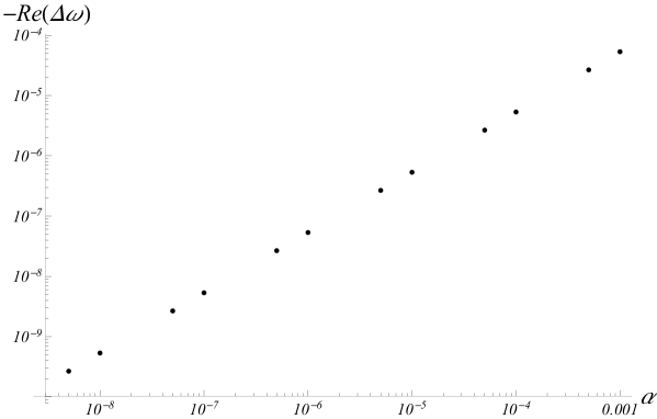
Figure 5: The log-log plot of the $-\Re(\Delta\omega)$ part of the gravitational fundamental mode $(\ell=2,n=0)$ for $\alpha=5\times 10^{-9},10^{-8},5\times 10^{-8},10^{-7},5\times 10^{-7},\dots,10^{-3}$

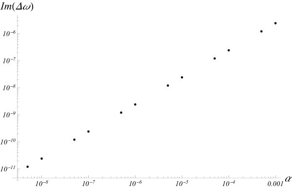
Figure 6: The log-log plot of the $\Im(\Delta\omega)$ part of the gravitational fundamental mode $(\ell=2,n=0)$ for $\alpha=5\times 10^{-9},10^{-8},5\times 10^{-8},10^{-7},5\times 10^{-7},\dots,10^{-3}$

III.3 The second-order solution

Finally, let us consider the influence of the second-order solution of the equations (5) and (6) upon the quasinormal modes. Now, for $m(r)$ and $\psi(r)$ one has

$$m(r)=\mathcal{M}-\alpha\frac{4\mathcal{M}^{2}}{r^{6}}\left(49\mathcal{M}-27r\right)+\frac{24\alpha^{2}\mathcal{M}^{4}(6787\mathcal{M}-4104r)}{11r^{12}}$$ (40)

and

$$\psi(r)=-\alpha\frac{108\mathcal{M}^{2}}{r^{6}}+\frac{1296\alpha^{2}\mathcal{M}^{3}(253\mathcal{M}-128r)}{11r^{12}},$$ (41)

whereas the event horizon $r_{+}$ is located at

$$r_{+}=2\mathcal{M}\left(1+\frac{5\alpha}{16\mathcal{M}^{4}}-\frac{1623\alpha^{2}}{5632\mathcal{M}^{8}}\right).$$ (42)

Making use of Eq. (7) one obtains the following expression describing the effective potential

$$V(r) = \frac{1}{r}\left(1-\frac{2\mathcal{M}}{r}\right)\left(\frac{L}{r}-\frac{6\mathcal{M}}{r^{2}}\right)$$ (43)

$$-\frac{8\mathcal{M}^{2}\alpha}{r^{10}}\left(528\mathcal{M}^{2}-549\mathcal{M}r+5\mathcal{M}Lr+135r^{2}\right)$$

$$-\frac{48\alpha^{2}\mathcal{M}^{3}}{11r^{16}}\left(-29249L\mathcal{M}^{2}r+28728L\mathcal{M}r^{2}-6912Lr^{3}\right.$$

$$\left.+436656M^{3}-567867\mathcal{M}^{2}r+250128\mathcal{M}r^{2}-38016r^{3}\right).$$

Repeating the steps of Sec. III.2 one can construct the quasinormal frequencies. The results of our calculations are tabulated in Tab. 3. This time however, the calculations are more complex and time consuming as the construction of the derivatives of $V(x)$ could impose severe demands on the computer resources.

Table 3: The complex frequencies of the fundamental gravitational quasinormal modes of the dirty black hole with the second-order corrections calculated within the framework of the WKB-Padé technique. The geometry of the black hole is characterized by Eqs. (40) and (41).

$\ell$	$\omega$
2	$0.747290083278501734-0.177922209944631719i$
3	$1.198829835396153738-0.185412278758324958i$
4	$1.618293857305014600-0.188337388043360077i$
5	$2.024520040450694490-0.189752027161955573i$
6	$2.423940490052797489-0.190543512760709371i$
7	$2.819381986313369047-0.191031575267004615i$
8	$3.212289751605332245-0.191354039537637231i$
9	$3.603482171586300389-0.191578355817096047i$
10	$3.993458344812290014-0.191740758590793688i$

Inspection of tables 2 and 3 shows that the absolute value of the difference between the first and the second-order results is a few orders of magnitude smaller than the difference between the Schwarzschild and the first order results. Indeed, in the first case the difference of the real part does not exceed $1.5\times 10^{-7}$ whereas the imaginary part is always smaller than $3.5\times 10^{-8}.$ This can be contrasted with the first case, where the analogous differences are typically $10^{3}$ times bigger.

IV Final Remarks

In this paper, we have investigated the influence of the effective two-loops renormalizable gravity upon the quasinormal modes. The idealized “experimental” situation we have in mind is the following: we have two black holes characterized by the same mass $\mathcal{M}.$ One of them is described by the Schwarzschild line element whereas the second one has (presumable small) corrections caused by the Goroff-Sagnotti sixth-order curvature terms. Our task is to determine which black hole is which. We see that this question - when addressed naively - may lead to incorrect answer. Indeed, making use of unsophisticated claculational techniques one can obtain results in which the error of the method is bigger than the expected effect, so the results, although mathematically correct, do not reflect the actual situation. For example, $\Re(\omega)$ of the lowest fundamental mode of the dirty black hole clculated within the framework of the MSW method is closer to the exact Schwarzschild value than its uncorrected counterpart. Assuming that the coupling constant $\alpha$ is small all we need is a very accurate and sensitive method for calculations of the complex frequencies. In this paper we argue that the Padé approximants of the (formal) WKB series describing quasinormal frequencies of the black holes may have desired features. In the case in hand, one can easily approach the accuracy of, say, 30 decimal places (or more) even for low-lying modes. For example, both the continued fraction method and the WKB-Padé summation agree that to 32 digits accuracy

$$\omega=0.74734336883608367158698400595410-0.17792463137787139656092185436905i$$ (44)

for the lowest fundamental gravitational mode of the Schwarzschild black hole. Of course, the method have some limitations, but because of its simplicity we believe that it can be the method of choice in many calculations of this type. We have limited ourselves to the two-loop renormalizable effective gravity. It is clear that this approach is easily adaptable to other theories (not necessarily pure gravity) with the higher-order curvature terms and in many related problems.

Finally, a few words on the computational side of the problem are in order. The calculations can be roughly divided into the three parts. First, we calculate the derivatives of the potential with respect to the $x$ coordinate at $x_{0}.$ Although highly algorithmic, this stage (when performed analytically) can be both time and memory consuming. Subsequently we construct the $\tilde{\Lambda}$ functions and finally we calculate the Padé transforms of the WKB series. It should be noted that the time spent on calculations of the Padé transforms is only a small fraction of the total time of computations. On the other hand, for a given $N,$ the calculation time of the WKB series is practically insensitive to the type of the black hole. All the calculations presented in this paper can easily be completed on a budget laptop with 16 GB of RAM.

References

- Matyjasek and Opala (2017) J. Matyjasek and M. Opala, Phys. Rev. D96, 024011 (2017).
- Fiziev (2006) P. P. Fiziev, Class. Quant. Grav. 23, 2447 (2006).
- Fiziev (2019) P. P. Fiziev (2019), eprint arXiv:1912.13432.
- Hatsuda (2020a) Y. Hatsuda (2020a), eprint arXiv:2006.08957.
- Vishveshwara (1970) C. V. Vishveshwara, Phys. Rev. D1, 2870 (1970).
- Kokkotas and Schmidt (1999) K. D. Kokkotas and B. G. Schmidt, Living Rev. Rel. 2, 2 (1999).
- Nollert (1999) H.-P. Nollert, Class. Quant. Grav. 16, R159 (1999).
- Konoplya and Zhidenko (2011) R. A. Konoplya and A. Zhidenko, Rev. Mod. Phys. 83, 793 (2011), eprint 1102.4014.
- Berti et al. (2009) E. Berti, V. Cardoso, and A. O. Starinets, Class. Quant. Grav. 26, 163001 (2009).
- Leaver (1985) E. W. Leaver, Proc. Roy. Soc. Lond. A402, 285 (1985).
- Nollert (1993) H.-P. Nollert, Phys. Rev. D 47, 5253 (1993).
- Rostworowski (2007) A. Rostworowski, Acta Phys. Polon. B38, 81 (2007).
- Majumdar and Panchapakesan (1989) B. Majumdar and N. Panchapakesan, Phys. Rev. D40, 2568 (1989).
- Cho et al. (2010) H. T. Cho, A. S. Cornell, J. Doukas, and W. Naylor, Class. Quant. Grav. 27, 155004 (2010).
- Jansen (2017) A. Jansen, Eur. Phys. J. Plus 132, 546 (2017).
- Nollert and Schmidt (1992) H.-P. Nollert and B. G. Schmidt, Phys. Rev. D 45, 2617 (1992).
- Schutz and Will (1985) B. F. Schutz and C. M. Will, Astrophys. J. 291, L33 (1985).
- Iyer and Will (1987) S. Iyer and C. M. Will, Phys. Rev. D35, 3621 (1987).
- Iyer (1987) S. Iyer, Phys. Rev. D35, 3632 (1987).
- Kokkotas and Schutz (1988) K. D. Kokkotas and B. F. Schutz, Phys. Rev. D37, 3378 (1988).
- Seidel and Iyer (1990) E. Seidel and S. Iyer, Phys. Rev. D41, 374 (1990).
- Froeman et al. (1992) N. Froeman, P. O. Froeman, N. Andersson, and A. Hoekback, Phys. Rev. D45, 2609 (1992).
- Andersson and Linneaus (1992) N. Andersson and S. Linneaus, Phys. Rev. D46, 4179 (1992).
- Konoplya (2003) R. A. Konoplya, Physical Review D 68, 024018 (2003).
- Gal’tsov and Matiukhin (1992) D. V. Gal’tsov and A. A. Matiukhin, Class. Quant. Grav. 9, 2039 (1992).
- Zaslavskii (1991) O. B. Zaslavskii, Phys. Rev. D43, 605 (1991).
- Blome and Mashhoon (1984) H. Blome and B. Mashhoon, Physics Letters A 100 (1984).
- Ferrari and Mashhoon (1984a) V. Ferrari and B. Mashhoon, Phys. Rev. Lett. 52, 1361 (1984a).
- Ferrari and Mashhoon (1984b) V. Ferrari and B. Mashhoon, Phys. Rev. D30, 295 (1984b).
- Matyjasek and Telecka (2019) J. Matyjasek and M. Telecka, Phys. Rev. D 100, 124006 (2019).
- Myers (1999) R. C. Myers, in Black holes, gravitational radiation and the universe (Kluwer Acad. Publ., Dordrecht, 1999).
- Lu and Wise (1993) M. Lu and M. B. Wise, Phys. Rev. D47, 3095 (1993).
- Matyjasek et al. (2006) J. Matyjasek, M. Telecka, and D. Tryniecki, Phys. Rev. D73, 124016 (2006).
- Dobado and Maroto (1993) A. Dobado and A. L. Maroto, Phys. Lett. B 316, 250 (1993).
- Konoplya et al. (2020) R. Konoplya, A. Zinhailo, and Z. Stuchlik, Phys. Rev. D 102, 044023 (2020).
- Momennia and Hendi (2020) M. Momennia and S. H. Hendi, Eur. Phys. J. C 80, 505 (2020).
- Bouhmadi-López et al. (2020) M. Bouhmadi-López, S. Brahma, C.-Y. Chen, P. Chen, and D.-h. Yeom, JCAP 2007, 066 (2020).
- Matyjasek (2001) J. Matyjasek, Phys. Rev. D63, 084004 (2001).
- Matyjasek (2004) J. Matyjasek, Phys. Rev. D70, 047504 (2004).
- Medved et al. (2004a) A. Medved, D. Martin, and M. Visser, Class. Quant. Grav. 21, 1393 (2004a).
- Medved et al. (2004b) A. Medved, D. Martin, and M. Visser, Class. Quant. Grav. 21, 2393 (2004b).
- ’t Hooft and Veltman (1974) G. ’t Hooft and M. Veltman, Ann. Inst. H. Poincare Phys. Theor. A 20, 69 (1974).
- Goroff and Sagnotti (1985) M. H. Goroff and A. Sagnotti, Phys. Lett. B 160, 81 (1985).
- Goroff and Sagnotti (1986) M. H. Goroff and A. Sagnotti, Nucl. Phys. B 266, 709 (1986).
- (45) B. Mashhoon, in Third Marcel Grossmann Meeting on General Relativity (North-Holland, Amsterdam, 1983).
- Matyjasek (2004b) J. Matyjasek, Phys. Rev. D 70, 047504 (2004b).
- Berej et al. (2006) W. Berej, J. Matyjasek, D. Tryniecki, and M. Woronowicz, Gen. Rel. Grav. 38, 885 (2006).
- Bender and Orszag (1978) C. M. Bender and S. A. Orszag, Advanced mathematical methods for scientists and engineers (McGraw-Hill, New York, 1978).
- Hatsuda (2020b) Y. Hatsuda, Phys. Rev. D 101, 024008 (2020b).
- Sulejmanpasic and Ünsal (2018) T. Sulejmanpasic and M. Ünsal, Comput. Phys. Commun. 228, 273 (2018).