Using Unsupervised Learning to Help Discover the Causal Graph

Abstract

The software outlined in this paper, AitiaExplorer, is an exploratory causal analysis tool which uses unsupervised learning for feature selection in order to expedite causal discovery. In this paper the problem space of causality is briefly described and an overview of related research is provided. A problem statement and requirements for the software are outlined. The key requirements in the implementation, the key design decisions and the actual implementation of AitiaExplorer are discussed. Finally, this implementation is evaluated in terms of the problem statement and requirements outlined earlier. It is found that AitiaExplorer meets these requirements and is a useful exploratory causal analysis tool that automatically selects subsets of important features from a dataset and creates causal graph candidates for review based on these features. The software is available at https://github.com/corvideon/aitiaexplorer

I Introduction

Causality has become a major research interest in the field of machine learning. Although collecting vast amounts of data leads to the creation of useful systems, in order to truly understand the data one needs to understand the causes and effects that are implicit in the data. As Peters et al. (2017) point out, causal reasoning is actually “more powerful” than just using probabilistic and statistical reasoning alone. Unlocking causality will allow our machine learning systems to do more with the data available.

The software outlined in this paper, AitiaExplorer (from the Ancient Greek for cause, aitía), directly addresses this need to unlock causality within our systems. AitiaExplorer is an exploratory causal analysis (ECA) tool which uses unsupervised learning for feature selection in order to expedite causal discovery. Exploratory causal analysis is an initial first step in the causal analysis of a system, a causal counterpart to exploratory data analysis. ECA can be at least partially automated and the results can guide more formal causal analysis.

Feature selection methods are used in data analysis to suggest subsets of features that reduce dimensionality while minimising information loss. These methods can be divided into standard (or “classical”) feature selection methods and causal feature selection methods. Classical feature selection methods identify subsets of features using non-causal correlations. Causal feature selection methods seek to identify subsets of features by capturing actual casual relationships between selected features. However, [45] argue that both “causal and non-causal feature selection have the same objective”. This research suggests that even though classical feature selection methods have a different methodology to causal feature selection methods, they both work by exploiting common underlying structures in the data. Unfortunately, causal feature selection methods are less computationally efficient than classical feature selection methods and causal feature selection is still an active area of research. Classical feature selection is much better understood and the algorithms are generally faster. This is why AitiaExplorer provides an easy way to exploit standard feature selection methods as part of exploratory causal analysis (ECA) rather than causal feature selection methods.

One of the main outputs of ECA are causal graphs. Causal graphs are a useful tool in exploring causality but creating the correct causal graph is difficult. AitiaExplorer facilitates straightforward causal exploration of even quite large datasets by automatically creating causal graphs of subsets of the features of the dataset.

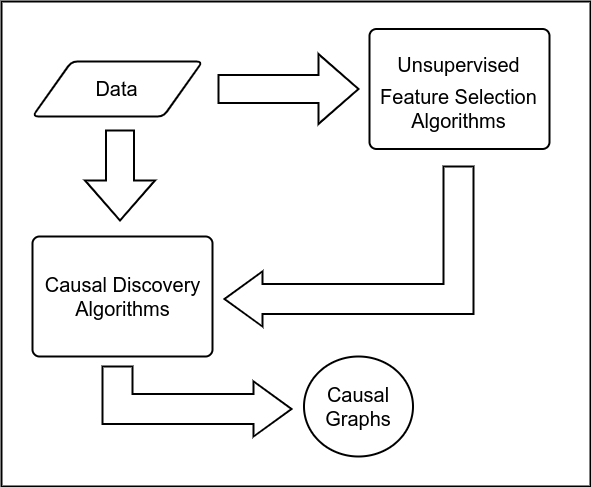
Figure 1: System overview.

This paper makes the following contributions:

• An overview and evaluation of the AitiaExplorer system which contains an ensemble of both causal discovery algorithms (responsible for creating the causal graphs) and an ensemble of unsupervised feature selection algorithms (responsible for automatically selecting the most important features). The two ensembles work together as outlined in Figure 1.

• The use of clustering analysis for feature selection via Principal Feature Analysis.

• The innovative use of standard supervised learning algorithms to allow their use in unsupervised feature selection. This is achieved by using synthetic data generated via a Bayesian Gaussian Mixture model.

• The ability of AitiaExplorer to create causal graphs from a dataset when no known target causal graph is provided.

• The ability of AitiaExplorer to automatically provide insights into latent unobserved variables in a causal graph.

This paper is structured as follows: In Section 2, the problem space of causality is described and a concise problem statement is provided. In Section 3, an overview of related research is provided. In Section 4, key requirements in the implementation of AitiaExplorer are discussed and in Section 5 the key design decisions behind AitiaExplorer are explored. In Section 6, the actual implementation of AitiaExplorer is described and in Section 7, this implementation is evaluated in terms of the problem statement and requirements outlined earlier.

II Background

II-A What is Causation?

The dictionary definition of causation (or more correctly causality) is “the act or agency which produces an effect” or the “connection between two events or states such that one produces or brings about the other”. This is certainly close to the intuitive, idiomatic idea of causation that one uses in daily life. An action produces an effect. For example, the rain caused the grass to be wet. The act of walking in a puddle without shoes causes my feet to get wet.

Philosophers have argued over the metaphysics of causality for nearly two millennia and modern psychology has added more layers of ambiguity to these discussions. This level of discussion is very interesting but a simpler definition will suffice for this article. The definition used in this document is that given by Pearl et al. (2016):

“A variable X is a cause for a variable Y if Y in any way relies on X for its value”.

This definition will cover intuitive everyday ideas of causality (for example, the grass relies on the rain for its wetness) and will also cover causal graphs later, where X and Y will express variables in a more formal causal inference.

II-B Causation and the Sciences

To many in the sciences during the early twentieth century, there was “a general suspicion of causal notions [which] pervaded a number of fields outside of philosophy, such as statistics and psychology”. However, despite efforts to banish causality from statistical research in fields such as medicine, many scientists continued to attempt to answer causal questions, despite having inadequate statistical training. As Hernan et al. put it, even today “confusions generated by a century-old refusal to tackle causal questions explicitly are widespread in scientific research”. However, causality has become a mainstream concern for scientists. In the words of one author, now it seems that we are all becoming social scientists as the causal analysis techniques that were widely used in social and biological research are moving into other fields such as machine learning.

II-C Competing Methods of Learning Causality

Unfortunately, for a student of machine learning entering the field of causality, there still seems to be no general agreement on what way is appropriate and correct for approaching causal inference. Depending on the field, whether it be social science, biological science or statistics, there are overlapping definitions and competing claims on what is most important. In a review of the available methods of learning causality, Guo et al. (2018) point out that “… the two most important formal frameworks … [are] … the structural causal models and the potential outcome framework[s]…” (emphasis added). However, if we consult another review of the available methods in Lattimore and Ong (2018), we find that they break down the competing schools of causality into counterfactuals (Neyman–Rubin), Structural Equation Models and causal Bayesian networks, with a short mention of Granger causality. As we can see, even in two recent review papers of the field, there are multiple competing naming conventions.

II-D Causal Model Framework (CFM)

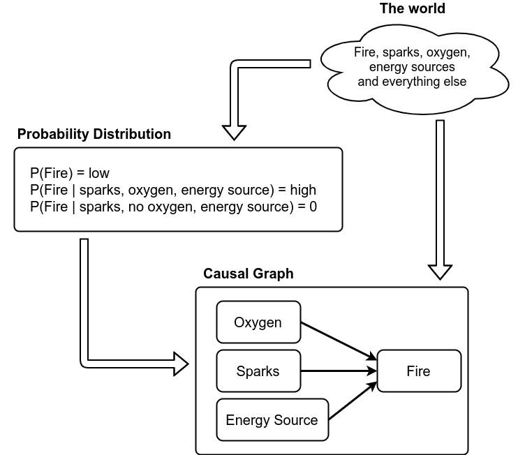
Figure 2: Causal Model Framework.

This document will use what Steven Sloman calls the “causal model framework”. This framework unites many of the disparate causal elements identified above into one scheme. He points out that this model is first described in 1993 and then completed in the work of Judea Pearl. The causal model framework consists of three entities:

1. A representation of the state of a system. This generally means some kind of dataset which acts as a proxy for the system.

2. A probability distribution that describes the causal connections in the dataset.

3. A causal graph depicting this dataset.

From this description we can see that any useful causal discovery tool needs to support these three entities.

The major advantage of using the causal model framework (CMF) is that using this scheme bypasses much of the confusing causal terminology that is used across several dozen scientific fields from genomics to social science. CMF allows a student of machine learning to use Bayesian networks, Structural Equation Models (SEM) and even potential outcomes (which are normally seen as an alternative, if not competition to SEM) in modelling a causal system. What brings all of these methods together in CMF is the causal graph. See Figure 2 for an illustration of CMF.

II-E What is a Causal Graph?

In general, causal graphs are graphical models that are used to provide formal and transparent representation of causal assumptions. They can be used for inference and testing assumptions about the underlying data. They can also be known as path diagrams or causal Bayesian networks.

More formally in CMF, a causal graph or graphical causal model consists of a directed acyclic graph (DAG) where an edge between nodes $X$ and $Y$ represents a function $f_{Y}$ that assigns a value to $Y$ based on the value of $X$. We can say in this case that $X$ is a cause of $Y$. In general, parent nodes are causes of child nodes. For a quick and thorough look at the relationship between all these terms see An Introduction to Causal Inference by Pearl.

For instance, in the example graph in Figure 3, one can see that the edge between nodes $sprinkler$, $rain$ and $wet$ represents a function $f_{wet}$ that assigns a value to $wet$ based on the value of $rain$ and $sprinkler$. You can see that $rain$ and $sprinkler$ are both causes of $wet$.

Figure 3: Example causal graph.

II-F Causal Inference, Causal Discovery and Learning Causality

The causal model (also known as a Structural Causal Model) underlying the causal graph is the conceptual model that describes the causal mechanisms of the system, i.e. the functions represented above by the edges of the causal graph. In CMF, the causal model is captured in the probability distributions that describe the underlying causal connections in the data.

But a causal model can be expressed with or without or a causal graph. For example, a set of Structural Equation Models (SEM) can describe the causal mechanisms of a system without a causal graph.

If one has a causal graph and a causal model for a system, this means that one has a comprehensive overview of the causal structure of that system. Guo et al. (2018) call the process of finding the causal graph causal discovery and the process of working with the causal model causal inference. Both of these terms come under the more general term of learning causality. There are other ways of defining these terms of course, but in general this is a useful distinction to make as it allows for more clarity in refining the research problem of this document.

II-G How a Causal Discovery Algorithm Works

To understand the causal model framework and learning causality in a little more depth, it is useful to consider the logic behind one of the first causal discovery algorithms, the IC Algorithm (Inductive Causation).

The relationship between a causal model and the real world system is the joint probability distribution over the variables in the system. Within the causal model framework, there are two assumptions made concerning this relationship:

1. The causal Markov condition which assumes that the direct causes of a variable, i.e. its parents, make it probabilistically independent of other variables in the system. Once one knows the values of the parental causes, there is no need to go back though long chains of indirect causes to find the value of a variable.

2. The stability or faithfulness assumption which assumes that the probabilistic independencies captured in the causal graph are because of an underlying causal structure and not just randomness.

One of the outcomes of these assumptions is the criterion of d-separation (where the d stands for dependence). Consider three sets of nodes in a causal graph $X$, $Y$ and $Z$. Set $Z$ is said to d-separate the nodes in $X$ from the nodes in $Y$ if and only if $Z$ blocks all paths (edges), and hence information, from a node in $X$ to a node in $Y$.

Consider the example graph from Figure 3:

• geographic position and Earth’s tilt are causally independent.

• season, sprinkler, rain and wet are causally dependent on geographic position and Earth’s tilt.

• geographic position and Earth’s tilt are direct causes of season (an example of a $v$-structure).

• geographic position and Earth’s tilt are indirect causes of sprinkler, rain and wet.

• If season is fixed, for example to "Winter", i.e. changes are prevented to geographic position and Earth’s tilt, then geographic position and Earth’s tilt will no longer cause changes in sprinkler, rain and wet. This is also called blocking or controlling for the season node.

• Node sprinkler can be said to be d-separated (and hence conditionally independent) from node rain when we control for the season node.

The criteria of d-separation can be used to generate a causal graph by calculating the various joint probability distributions over the pairs of variables in a dataset. This is how the IC Algorithm generates a partial directed acyclic graph (PDAG, a graph where the direction of some edges is ambivalent).

IC Algorithm (Inductive Causation) Input: $\hat{P}$, a stable probability distribution on a set of variables $V$. Output: A PDAG $H(\hat{P})$, compatible with $\hat{P}$. 1. For each pair of variables $a$ and $b$ in $V,$ search for a set $S_{ab}$ such that $(a\perp b\mid S_{ab})$ holds in $\hat{P}.$ This means $a$ and $b$ should be independent in $\hat{P}$, or d-separated, when conditioned on $S_{ab}$. Create a DAG $G$ such that the vertices $a$ and $b$ are connected with an edge if and only if no set $S_{ab}$ can be found. 2. For each pair of nonadjacent variables $a$ and $b$ with a common neighbour $c$, check if $c\in S_{ab}$. • If it is, then continue. • If not, then add directed edges pointing at $c$ i.e. $a\rightarrow c\leftarrow b$. 3. In the PDAG that results, orient as many of the undirected edges as possible, subject to these two conditions: • The orientation should not create a new $v$-structure. • The orientation should not create a directed cycle.

Of course, there are other ways of discovering the causal graph (see Section VI(E) for more details on the algorithms included in AitiaExplorer). But the IC algorithm illustrates the close connection between the causal model (understood as the joint probability distribution in the system) and the causal graph.

II-H Motivation for AitiaExplorer

The main problem with causal discovery is captured by Hyttinen et al. (2016):

“ … full knowledge of the true [causal] graph requires a rather extensive understanding of the system under investigation. Data alone is in general insufficient to uniquely determine the true causal graph. Even complete discovery methods will usually leave the graph under determined.”

Finding the causal graph of a system, or causal discovery, is difficult. Even if your causal discovery method creates an interesting graph, the graph may not be unique. This is because the graph may be a member of a set of possibly Markov-equivalent structures, each of which would satisfy the data.

However, there is some consolation:

“Algorithms that search for causal structure information … do not generally pin down all the possible causal details, but they often provide important insight into the underlying causal relations…” (emphasis added).

So this is an important motivation of AitiaExplorer and bolsters the claim that AitiaExplorer enables exploratory causal analysis. AitiaExplorer assists in the creation of causal graphs and can therefore provide important insights into underlying causal structures.

This insight provides AitiaExplorer with a simple problem statement.

Problem Statement Input: A dataset with a large number of features and with no known causal graph. Task: To automatically select subsets of important features from the dataset and create causal graphs candidates for review based on these features. Then provide a metric to compare these candidate causal graphs.

III Related Research

III-A Causal Inference in Current Machine Learning Research

There are many papers available in causal inference in machine learning research as this is currently a popular topic for research. In order to ascertain an idea of the amount of new research that is carried out in this area, see the GitHub repository associated with [13]. For this reason, it is quite difficult to isolate the current “state of the art” approach. However, each machine learning approach does seem to have its own causal learning experiments, as one can see in the selection of papers that are mentioned below. These papers were interesting but differ from the approach that is undertaken in this research:

Bengio et al. train a deep learning network on labelled causal data and allow the system to exploit small changes in probability distributions during interventions to identify causal structures. As this method uses labelled data, it does not fulfil the requirements of the current work and will be left to one side.

Dasgupta et al. uses a recurrent neural network with reinforcement learning in tasks with different causal structures. As they note, their research is “the first direct demonstration that causal reasoning can arise out of model-free reinforcement learning”. They note “traditional formal approaches usually decouple the problems of causal induction (inferring the structure of the underlying model from data), and causal inference (estimating causal effects based on a known model)”. However their work does not decouple these tasks (the use of causal induction here is what this document refers to as causal discovery). This use of reinforcement learning is highly attractive as it is model free. However this approach will be left to one side in this work in favour of less complex unsupervised methods.

Kalainathan et al. present a new approach to causal learning called the Structural Agnostic Model (SAM) which uses several different causal learning techniques within a Generative Adversarial Neural network. They claim that this provides a robust approach that has the advantages of multiple other techniques combined. However, as this paper is concentrating on unsupervised learning, the GAN approach will not be considered.

Bucur et al. offer an interesting approach from genetic research. They attempt to predict the causal structure of Gene Regulatory Networks (GRNs) using the covariance values in the genetic data alongside existing background knowledge of the genetic data priors to feed a Bayesian algorithm. This research is illustrative of the wide applicability of causal methods in many disciplines but it is too narrow in scope to provide much assistance to the research in this document.

III-B Complementary Causal Inference Research

There have been multiple papers published in the last few years in learning causality that share some of the same objectives as this work.

The paper from Pashami et al. discusses “the potential benefits, and explore[s] the hints that clusters in the data can provide for causal discovery”. This research provides some of the inspiration for AitiaExplorer, in that unsupervised learning can provide, at the very least, some heuristics for causal inference.

The work of Borboudakis and Tsamardinos on ETIO (from the Greek word for “cause”), a new “general causal discovery algorithm”, is in the same spirit as the research outlined in this document. The authors create this tool for what they call “integrative causal discovery” which is in keeping with the pragmatic ensemble approach suggested for AitiaExplorer.

Lin and Zhang explore the limitations of causal learning while also still retaining statistical consistency. They outline a new learning theory that may provide some ballast for a more general, ensemble approach to causal learning when they say “we should look for what can be achieved, and achieve the best we can”.

IV Requirements

IV-A Strategy

The strategy behind AitiaExplorer is to create an exploratory causal analysis (ECA) tool which will provide meaningful causal heuristics in the causal analysis of a specific dataset.

This will satisfy the problem statement defined in Section 2.7.

IV-B Primary Requirements

The development of AitiaExplorer will be subject to the following requirements, which follow on from the ECA discussion above:

• The software must place emphasis on augmenting human causal discovery in a pragmatic way.

• The software must be automated, at least partially.

These more technical requirements follow on from the problem statement:

• The software must be able to handle datasets with multiple features and no known causal graph.

• The software must be able to create multiple causal graphs and provide a way to compare these causal graphs.

Due to the time scale and resources available for the development of the software, the following will also apply:

• The software must make use of existing libraries and technology stacks.

• The software must be open source.

IV-C Secondary Requirements

The development of AitiaExplorer will be subject to the following requirements, which follow on from the primary requirements above:

• As the software needs to be at least partly automated, it follows therefore that only unsupervised learning is an option. This means no labelled data is required.

• The software will need little or no data preparation work (beyond the usual, such as scaling or encoding).

• The software will not need specialist hardware such as GPUs (graphics processing unit).

• The software will take an ensemble approach, allowing multiple algorithms to be tested in one pass.

For this reason, certain trends in current machine learning are not pursued, as outlined above.

V Key Design Decisions

V-A Programming Language Choice

There are several probabilistic programming languages available and these seemed like interesting choices for implementing a causal discovery tool.

Several candidates were reviewed:

• Pyro - A universal probabilistic programming language written in Python.

• Infer.NET - A .NET framework for probabilistic programming.

• Gen - A general-purpose probabilistic programming system with programmable inference.

In the end, useful as these languages are for generic probabilistic programming, none of the choices contained sufficient support for learning causality. Most of the existing causal-related software is implemented in Python (rather than in a subset of Python such as Pyro), so it was deemed more appropriate for AitiaExplorer to be written directly in Python.

V-B Causal Discovery Components

After reviewing many causality-related software packages, several were identified as being particularly useful for AitiaExplorer.

• Amongst these, the Tetrad Project appeared to be promising as this contains many causal discovery algorithms. Unfortunately Tetrad is implemented in Java which it makes unsuitable for AitiaExplorer. However, a Python package called py-causal exposes these causal discovery algorithms via a Java-Python communication layer. AitiaExplorer wraps the causal discovery algorithms provided by py-causal.

• The package CausalGraphicalModels was selected for displaying and manipulating causal graphs in Jupyter Notebooks due to its simplicity and elegance.

• The package pyAgrum provides two algorithms used internally in AitiaExplorer:

  • A target causal graph as supplied to AitiaExplorer represents the full causal model contained within the dataset. Sometimes this is known, but more often it is not. The greedy hill climbing algorithm provided by pyAgrum is used to approximate causal graphs when no target causal graph is provided. In theory, any causal discover algorithm could be used as a benchmark in this case (see Section VI for more details). However the algorithm used by pyAgrum is written in C++ and is very fast which makes it an excellent choice.

  • The MIIC (Multivariate Information based Inductive Causation) exposed by pyAgrum is used to identify latent unobserved edges in causal graphs. There does not seem to be many implementations of this algorithm (or similar) available in Python. Most implementations are in R.

V-C Unsupervised Learning for Feature Selection and Extraction

Although the approach using clustering as a causal heuristic in [27] is very interesting, it is beyond the scope of this particular research and does not provide a suitably pragmatic solution for AitiaExplorer.

Instead, two approaches using feature selection and extraction were identified as being suitable for AitiaExplorer:

1. The use of clustering via Principal Feature Analysis to select important features.

2. The use of standard supervised learning algorithms in an unsupervised manner as outlined below in the Design and Implementation section. These unsupervised versions of the algorithms can then be used for feature selection.

V-D Causal Graph Comparison Metrics

In order to allow AitiaExplorer to compare causal graphs, AitiaExplorer provides two metrics, Structural Hamming Distance (SHD) and Area Under the Precision-Recall Curve (AUPRC). Both of these metrics are reasonably quick and an implementation of each was available in Python. These measurements are provided in AitiaExplorer, with an emphasis on SHD.

VI Implementation

VI-A Design Overview

A high level design for the AitiaExplorer system can be seen in the Figure 4 below. The system design is based loosely on the design of the system outlined in Hyttinen et al. (2016).

• (A) The data to be analysed is passed in as a Pandas Dataframe. If a target causal graph is supplied, this is used as a benchmark for measuring all causal graphs generated by the system. If no target causal graph is provided, the system assumes that it is unknown and a target causal graph is generated from the data. This is then used as a proxy benchmark by the system.

• (B) The data is passed to the ensemble of unsupervised feature selection algorithms.

• (C) Each unsupervised feature selection algorithm selects what it considers to be the most important features.

• (D) The selected features from each unsupervised feature selection algorithm are made available to the causal discovery algorithms.

• (E) The data is passed to the ensemble of causal discovery algorithms.

• (F) Each causal discovery algorithm is run in turn with just the selected features from each unsupervised feature selection algorithm.

• (G) A set of causal graphs and associated metrics is outputted.

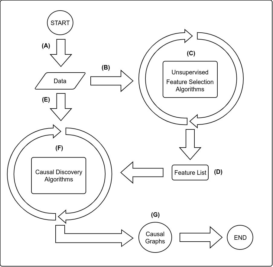
Figure 4: Overall structure of the system.

The software is implemented as a set of Python classes and can be used as either a Python library in an existing application, or as an analysis tool within a Jupyter Notebook.

VI-B Principal Feature Analysis

Principal Feature Analysis (PFA) is a method used for harnessing the dimensionality reduction ability of Principal Component Analysis (PCA) whilst also being able to identify the most important features that make up each principal component. In PFA, the data is clustered using PCA and then the components are fitted to a K-Means clustering algorithm. The most important features are those with the minimum euclidean distance from a cluster centre.

Principal Feature Analysis is available as one of the unsupervised feature selection methods in AitiaExplorer.

VI-C Turning Supervised Learning Algorithms into Unsupervised Learning Algorithms

Traditional supervised learning algorithms can be turned into unsupervised learning algorithms in the following way:

• Create suitable synthetic data from a reference distribution. In AitiaExplorer this is achieved by using a Bayesian Gaussian Mixture Model (BGMM). A BGMM can be used for clustering but it can also be used to model the data distribution that best represents the data. This means that a BGMM, when fitted to a specific dataset, can be used to provide sample data, allowing the creation of synthetic data.

• This synthetic data can then be combined with real data, along with an extra label that separates the synthetic data from the real data.

• This new dataset can then allow a classifier to be trained in an unsupervised manner.

• The supervised learning algorithm learns to distinguish the original data from the synthetic data.

The actual classification ability of the algorithms described above is not vitally important for AitiaExplorer. Instead, AitiaExplorer exploits the fact that as part of the training and classification cycle above, each algorithm internally selects and orders features in the dataset. AitiaExplorer puts the outputs of the classification process to one side and instead queries each algorithm for the features it considers to be the most important.

There are other choices for creating plausible synthetic data that would work e.g. using an autoencoder. However, the choice of BGMM is pragmatic as befits the AitiaExplorer requirements outlined in Section IV. The advantage of the BGMM is the actual scikit-learn implementation. This implementation is fast, simple to use and actually infers the effective number of clusters directly from the data.

Of course, multiple tools and techniques exist that could could be plugged into AitiaExplorer for feature selection. However, within the constraints of this research, the Bayesian Gaussian Mixture Model was found to be a good overall candidate that works well.

VI-D Feature Selection Algorithms Available in AitiaExplorer

The feature selection algorithms are listed in Table II. PFA (Principal Feature Analysis) is implemented internally in AitiaExplorer, XGBClassifier is provided as part of XGBoost and the remainder of the algorithms are provided through SKLearn.

Algorithm
Principal Feature Analysis (PFA)
XGBClassifier
Recursive Feature Elimination
Linear Regression
SGD Classifier
Random Forest Classifier
Gradient Boosting Classifier

Table I: Feature selection algorithms available in AitiaExplorer.

VI-E Causal Discovery Algorithms Available in AitiaExplorer

There are two main types of causal discovery algorithms. These are constraint-based algorithms and score based algorithms:

• Constraint-based algorithms build the graph by parsing the data and looking for independent conditional probabilities as described in Section II.

• Score-based methods search over a set of possible graphs that fits the data according to a metric.

AitiaExplorer allows the use of both types of causal discovery algorithms.

Algorithm	Description
bayesEst	Score-based - a revised Greedy Equivalence Search (GES) algorithm.
PC Algorithm	The original constraint-based algorithm.
FCI Algorithm	Constraint-based algorithm.
FGES Algorithm	Score-based - optimised and parallelised Greedy Equivalence Search (GES).
GFCI Algorithm	Hybrid - a combination of the FGES and the FCI algorithm.
RFCI Algorithm	Constraint-based algorithm - a faster modification of the FCI algorithm.

Table II: Causal discovery algorithms available in AitiaExplorer.

VII Evaluation

The evaluations below are based on the requirements outlined in Section IV. Each scenario captures an illustration of how AitiaExplorer meets these requirements. All of these evaluations were carried out using AitiaExplorer running through a Jupyter Notebook.

VII-A Evaluating the Unsupervised Learning Algorithms

As explained earlier, AitiaExplorer uses supervised learning algorithms in an unsupervised manner. A selection of these algorithms were trained in this manner with data from the HEPAR II dataset combined with synthetic data. The results are displayed in Table III. Several of the classifiers have an almost perfect score on the dataset in separating the real data from the synthetic data. Even though the SGDClassifier does very poorly, it is still useful for feature selection. LinearRegression and Principal Feature Analysis have been omitted from this test as the score metric is not meaningful for these algorithms.

Algorithm	Score
SGDClassifier	0.	5004
RandomForestClassifier	1.	0
GradientBoostingClassifier	1.	0
XGBClassifier	1.	0

Table III: Unsupervised learning algorithm scores.

VII-B Evaluating Causal Discovery When No Causal Graph is Supplied

A target causal graph is important in AitiaExplorer because it offers the user a simple way of comparing causal graphs produced by the system. Each causal graph that is outputted has an Structural Hamming Distance (SHD) and Area Under the Precision-Recall Curve (AUPRC) score given against the target causal graph. When no target causal graph is supplied, as outlined in Section V(B), AitiaExplorer will generate a proxy target graph using a fast greedy hill climbing algorithm. The proxy target causal graph is not meant as a absolute measure of correctness, but rather as an heuristic for the user to be able to compare across causal graphs, independent of any specific combination of causal discovery / feature selection algorithm.

AitiaExplorer was run twice with data from the HEPAR II dataset. Both runs used the same parameters, except that in the first run the known target causal graph was supplied. In the second, no target graph was supplied, forcing AitiaExplorer to create a proxy target causal graph. The results from the first run with the known target causal graph are displayed in Table IV overleaf. The results from the second run with the proxy target causal graph are displayed in Table V overleaf. As one would expect, the SHD scores are higher and the AUPRC scores are lower in the second run. However, after a closer inspection the changes in values are consistent across both runs. The SHD values remain constant across all combinations in both runs. Also, the AUPRC from the Random Forest Classifier fare worse than other feature selection methods in both runs. These results verify that the target causal graph, created by AitiaExplorer in run number two, provides a reasonable proxy benchmark when no target causal graph is supplied. The differences between the runs are proportional and consistent.

Causal Algorithm	Feature Selection Method	AUPRC		SHD
PC	Linear Regression	0.	5101	99
FCI	Linear Regression	0.	5101	99
RFCI	Linear Regression	0.	5101	99
PC	Random Forest Classifier	0.	26505	99
FCI	Random Forest Classifier	0.	26505	99
RFCI	Random Forest Classifier	0.	26505	99
PC	Recursive Feature Elimination	0.	5101	99
FCI	Recursive Feature Elimination	0.	5101	99
RFCI	Recursive Feature Elimination	0.	5101	99

Table IV: Causal discovery when causal graph is supplied.

Causal Algorithm	Feature Selection Method	AUPRC		SHD
PC	Linear Regression	0.	51255	123
FCI	Linear Regression	0.	51255	123
RFCI	Linear Regression	0.	51255	123
PC	Random Forest Classifier	0.	01255	125
FCI	Random Forest Classifier	0.	01255	125
RFCI	Random Forest Classifier	0.	01255	125
PC	Recursive Feature Elimination	0.	51255	123
FCI	Recursive Feature Elimination	0.	51255	123
RFCI	Recursive Feature Elimination	0.	51255	123

Table V: Causal discovery when no causal graph is supplied.

VII-C Evaluating Causal Discovery with a Set Number of Features

AitiaExplorer allows one to select the number of features that are selected in the causal discovery process. In this example, AitiaExplorer was run with a combination of causal discovery / feature selection algorithms. For clarity and simplicity, a small simulated dataset was used and only 7 features of a possible 10 features were selected. The results from the run are displayed in Table VI below. The best results have a lower SHD and a higher AUPRC.

Run Index	Causal Algorithm	Feature Selection Method	AUPRC		SHD
0	PC	Linear Regression	0.	662500	8
1	FCI	Linear Regression	0.	662500	8
2	FGES	Linear Regression	0.	662500	8
3	GFCI	Linear Regression	0.	662500	8
4	RFCI	Linear Regression	0.	662500	8
5	PC	Principal Feature Analysis	0.	370313	10
6	FCI	Principal Feature Analysis	0.	370313	10
7	FGES	Principal Feature Analysis	0.	370313	10
8	GFCI	Principal Feature Analysis	0.	370313	10
9	RFCI	Principal Feature Analysis	0.	370313	10
10	PC	Random Forest	0.	495833	9
11	FCI	Random Forest	0.	370313	10
12	FGES	Random Forest	0.	370313	10
13	GFCI	Random Forest	0.	370313	10
14	RFCI	Random Forest	0.	370313	10
15	PC	Recursive Feature Elimination	0.	286979	11
16	FCI	Recursive Feature Elimination	0.	078125	12
17	FGES	Recursive Feature Elimination	0.	078125	12
18	GFCI	Recursive Feature Elimination	0.	078125	12
19	RFCI	Recursive Feature Elimination	0.	078125	12
20	PC	XGBoost	0.	286979	11
21	FCI	XGBoost	0.	286979	11
22	FGES	XGBoost	0.	286979	11
23	GFCI	XGBoost	0.	286979	11
24	RFCI	XGBoost	0.	286979	11

Table VI: Causal discovery with a set number of features.

One can in the plot the relationship between the SHD and the AUPRC as in Figure 5 above. In general, the lower SHD is associated with a higher AUPRC, suggesting that the combination of causal discovery / feature selection algorithms from earlier runs may be optimal. These results demonstrate a simple use case of AitiaExplorer which allows the user to fix the number of features and test multiple combinations of algorithms in one step. These combinations can then be compared for further exploration.

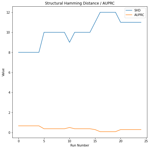
Figure 5: Causal discovery with a set number of features.

VII-D Evaluating Causal Discovery Within a Range of Features

AitiaExplorer allows one to select a numeric range of features that are selected in the causal discovery process. In this example, AitiaExplorer was run with a range of between 10 and 20 features from the HEPAR II dataset. The PC and FGES causal discovery algorithms and the Linear Regression and Random Forest feature selection algorithms were selected. AitiaExplorer then ran the selected combinations of algorithms across the data for each number of features, from 10 to 20. The results for the SHD and AUPRC values are graphed below in Figure 6 and Figure 7.

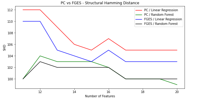
Figure 6: SHD - causal discovery with a range of features.

The results of this example are interesting because here a score-based causal discovery algorithm (PC) is pitted against a constraint-based causal discovery algorithm. Both causal discovery algorithms have a lower SHD when the number of features goes above 17. However, it appears that the AUPRC of the PC causal discovery algorithm is higher when used with the Random Forest Classifier. This knowledge can be used in further causal analysis. This example is an indication of how AitiaExplorer automatically provides a way of comparing multiple methods of producing a causal graph to see which is the most promising.

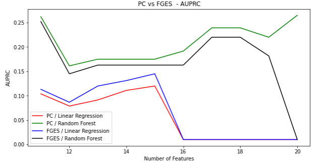
Figure 7: AUPRC - causal discovery with a range of features.

VII-E Evaluating Causal Discovery with Latent Unobserved Variables

The nodes in a causal graph are the observable or measured causal features. However, unobserved or latent variables can be inferred by certain causal discovery algorithms. These confounding variables (where the node is an unobservable common cause of two observable nodes) can be represented on a causal graph as an empty node as in Figure 8. In this example, the latent variable could be $hosepipe$ which could be a cause of both $ice$ and $wet$ depending on the season.

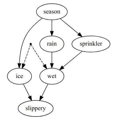
Figure 8: Example of a causal graph with latent edges.

AitiaExplorer will identify latent unobserved features in the causal discovery process as outlined in Section V(B). In this example, AitiaExplorer was run with a selection of 30 features from the HEPAR II dataset. Once the system has finished running the causal discovery process, once can display the causal graphs that contain latent unobserved features. A section of such a causal graph is displayed in Figure 9 above (highlight added). One can also get a list of the edges where these missing nodes are. In this case, these edges are identified as [(’Cirrhosis’, ’platelet’), (’Cirrhosis’, ’alcoholism’)]. These values can then be used in further analysis, as required.

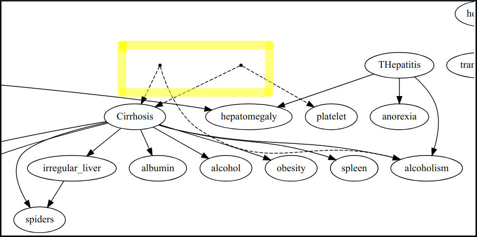
Figure 9: A causal graph with latent unobserved edges.

VII-F Achievement of Requirements

AitiaExplorer can now be evaluated as to whether it meets the primary and secondary requirements as outlined in Section IV.

VII-F1 Primary Requirements

• The software must place emphasis on augmenting human causal discovery in a pragmatic way: AitiaExplorer meets this requirement. The examples in this section illustrate how AitiaExplorer is an exploratory causal analysis, extending the ability of a user to explore the causal structures inherent in a given dataset.

• The software must be automated, at least partially: AitiaExplorer meets this requirement. As shown in Sections VII(B), VII(C) and VII(D), AitiaExplorer just needs the user to pass in the required parameters and the system will do the rest.

• The software must be able to handle datasets with multiple features and no known causal graph: AitiaExplorer meets this requirement. Several of the examples here use the HEPAR II dataset which contains ten thousand records and seventy feature nodes.

• The software must be able to create multiple causal graphs and provide a way to compare these causal graphs: AitiaExplorer meets this requirement. As shown in Sections VII(C) and VII(D), AitiaExplorer provides the SHD and AUPRC metrics for each combination of algorithm. These values are returned in a dataframe and can be plotted using standard Python tools in a Jupyter Notebook.

• The software must make use of existing libraries and technology stacks: AitiaExplorer meets this requirement. AitiaExplorer relies upon several open source Python frameworks as outlined in Section V.

• The software must be open source: AitiaExplorer meets this requirement. The source code is available on GitHub under a permissive open source license.

VII-F2 Secondary Requirements

• As the software needs to be at least partly automated, it follows therefore, that only unsupervised learning is an option: AitiaExplorer meets this requirement. All feature selection algorithms used are unsupervised. No labelled training data is required.

• The software will need little or no data preparation work: AitiaExplorer meets this requirement. AitiaExplorer accepts a dataset in a standard Pandas Dataframe.

• The software will not need specialist hardware such as GPUs: AitiaExplorer meets this requirement. All evaluations were run on a laptop without the use of a GPU and most were completed in under an hour.

• The software will take an ensemble approach, allowing multiple algorithms to be tested in one pass: AitiaExplorer meets this requirement. AitiaExplorer will take an arbitrary number of causal discovery and feature selection algorithms, once they are defined with the system.

VIII Conclusion

AitiaExplorer provides an efficient solution to the problem statement from Section 2.7. The software is a useful exploratory causal analysis tool that automatically selects subsets of important features from a dataset and creates causal graph candidates for review based on these features. A metric is also provided to compare these candidate causal graphs.

VIII-A SWOT Analysis

VIII-A1 Strengths

• AitiaExplorer met the requirements for an exploratory causal analysis as set out in Section IV.

• AitiaExplorer demonstrates that one can build a system that augments the ability of a user to find candidate causal graphs efficiently.

• The Python language and ecosystem is an excellent choice for this kind of project. The availability of many excellent causality-related libraries is a major advantage. Working within a Jupyter Notebook with AitiaExplorer is very straightforward and productive.

VIII-A2 Weaknesses

• Causal discovery is still very difficult without an extensive understanding of the system under investigation. Many of the causal graphs returned by AitiaExplorer are poor candidates. This is part of the challenge of causal discovery.

• The SHD and AUPRC metrics as provided by AitiaExplorer are useful, but only provide a shallow comparison metric between graphs. With more time and resources, better comparison metrics with more detailed analysis could be provided.

VIII-A3 Opportunities

• AitiaExplorer could be extended in several interesting ways, perhaps to allow further analysis of causal models. As per the terminology outlined in Section II(F), AitiaExplorer is primarily a causal discovery tool and works on the level of causal graphs. With more time and resources, AitiaExplorer could become a causal inference tool also, and allow analysis of the underlying causal models behind the causal graphs.

• A version of AitiaExplorer with causal feature selection methods alongside classical feature selection methods for comparison would be a very interesting and potentially useful research project.

VIII-A4 Threats

• AitiaExplorer was tested against reasonably large datasets and worked efficiently. However, some of the datasets where exploratory causal analysis would be really useful are very large indeed, often with thousands of features and hundreds of thousands of records. It is unknown how well AitiaExplorer would perform under this type of workload.

VIII-B Future Work

It was hoped that AitiaExplorer could be extended to include support for the DoWhy calculus of Judea Pearl which would open up the ability for AitiaExplorer to explore counterfactual causal graphs and perhaps compare scenarios of several candidate graphs. It was also desirable to include some different, more innovative algorithms in AitiaExplorer, such as the NOTEARS algorithm and the Boruta algorithm. However, due to time and resource constraints, this interesting work will have to be carried out at a future time.

VIII-C Acknowledgements

The author would like to thank Dr. Alessio Benavoli and Dr Pepijn van de Ven for their professional advice and support.

References

- [1] John T. Behrens “Principles and Procedures of Exploratory Data Analysis” In Psychological Methods 2.2 US: American Psychological Association, 1997, pp. 131–160 DOI: 10.1037/1082-989X.2.2.131
- [2] Yoshua Bengio et al. “A Meta-Transfer Objective for Learning to Disentangle Causal Mechanisms”, 2019 arXiv: http://arxiv.org/abs/1901.10912
- [3] Kenneth A. Bollen “Structural Equation Models” In Encyclopedia of Biostatistics American Cancer Society, 2005 DOI: 10.1002/0470011815.b2a13089
- [4] Kenneth A. Bollen and Judea Pearl “Eight Myths About Causality and Structural Equation Models” In Handbook of Causal Analysis for Social Research Dordrecht: Springer Netherlands, 2013, pp. 301–328 DOI: 10.1007/978-94-007-6094-3_15
- [5] Giorgos Borboudakis and Ioannis Tsamardinos “Towards Robust and Versatile Causal Discovery for Business Applications” In Proceedings of the 22Nd ACM SIGKDD International Conference on Knowledge Discovery and Data Mining, KDD ’16 New York, NY, USA: ACM, 2016, pp. 1435–1444 DOI: 10.1145/2939672.2939872
- [6] Kendrick Boyd, Kevin H. Eng and C. Page “Area under the Precision-Recall Curve: Point Estimates and Confidence Intervals” In Machine Learning and Knowledge Discovery in Databases, Lecture Notes in Computer Science Berlin, Heidelberg: Springer, 2013, pp. 451–466 DOI: 10.1007/978-3-642-40994-3_29
- [7] Ioan Gabriel Bucur, Tom Bussel, Tom Claassen and Tom Heskes “A Bayesian Approach for Inferring Local Causal Structure in Gene Regulatory Networks”, 2018 arXiv: http://arxiv.org/abs/1809.06827
- [8] David Chickering “Optimal Structure Identification With Greedy Search.” In Journal of Machine Learning Research 3, 2002, pp. 507–554 DOI: 10.1162/153244303321897717
- [9] Diego Colombo, Marloes H. Maathuis, Markus Kalisch and Thomas S. Richardson “LEARNING HIGH-DIMENSIONAL DIRECTED ACYCLIC GRAPHS WITH LATENT AND SELECTION VARIABLES” In The Annals of Statistics 40.1 Institute of Mathematical Statistics, 2012, pp. 294–321 JSTOR: 41713636
- [10] Ishita Dasgupta et al. “Causal Reasoning from Meta-Reinforcement Learning”, 2019 arXiv: http://arxiv.org/abs/1901.08162
- [11] Thompson Gale “Causation: Philosophy of Science | Encyclopedia.Com”, 2006 URL: https://www.encyclopedia.com/humanities/encyclopedias-almanacs-transcripts-and-maps/causation-philosophy-science
- [12] Justin Grimmer “We Are All Social Scientists Now: How Big Data, Machine Learning, and Causal Inference Work Together” In PS: Political Science & Politics 48.01, 2015, pp. 80–83 DOI: 10.1017/S1049096514001784
- [13] Ruocheng Guo et al. “A Survey of Learning Causality with Data: Problems and Methods”, 2018 arXiv: http://arxiv.org/abs/1809.09337
- [14] Miguel A. Hernan, John Hsu and Brian Healy “A Second Chance to Get Causal Inference Right: A Classification of Data Science Tasks” In CHANCE 32.1, 2019, pp. 42–49 DOI: 10.1080/09332480.2019.1579578
- [15] Antti Hyttinen and Frederick Eberhardt “Do-Calculus When the True Graph Is Unknown”, 2016 URL: https://core.ac.uk/display/103695128
- [16] Guido W. Imbens and Donald B. Rubin “Rubin Causal Model” In Microeconometrics, The New Palgrave Economics Collection London: Palgrave Macmillan UK, 2010, pp. 229–241 DOI: 10.1057/9780230280816_28
- [17] Amin Jaber, Jiji Zhang and Elias Bareinboim “Causal Identification under Markov Equivalence”, 2018 arXiv: http://arxiv.org/abs/1812.06209
- [18] Diviyan Kalainathan et al. “Structural Agnostic Modeling: Adversarial Learning of Causal Graphs”, 2019 arXiv: http://arxiv.org/abs/1803.04929
- [19] Miron B. Kursa and Witold R. Rudnicki “Feature Selection with the Boruta Package” In Journal of Statistical Software 36.11, 2010 DOI: 10.18637/jss.v036.i11
- [20] Finnian Lattimore and Cheng Soon Ong “A Primer on Causal Analysis”, 2018 arXiv: http://arxiv.org/abs/1806.01488
- [21] Hanti Lin and Jiji Zhang “How to Tackle an Extremely Hard Learning Problem: Learning Causal Structures from Non-Experimental Data without the Faithfulness Assumption or the Like”, 2018 arXiv: http://arxiv.org/abs/1802.07051
- [22] Yijuan Lu, Ira Cohen, Xiang Sean Zhou and Qi Tian “Feature Selection Using Principal Feature Analysis” In Proceedings of the 15th International Conference on Multimedia - MULTIMEDIA ’07 Augsburg, Germany: ACM Press, 2007, pp. 301 DOI: 10.1145/1291233.1291297
- [23] Daniel Malinsky and David Danks “Causal Discovery Algorithms: A Practical Guide” In Philosophy Compass 13.1, 2018, pp. e12470 DOI: 10.1111/phc3.12470
- [24] James M. McCracken “Exploratory Causal Analysis with Time Series Data” In Synthesis Lectures on Data Mining and Knowledge Discovery 8.1 Morgan & Claypool Publishers, 2016, pp. 1–147 DOI: 10.2200/S00707ED1V01Y201602DMK012
- [25] C. Meek “Causal Inference and Causal Explanation with Background, Uncertainty in Artificial Intelligence: Proc. of the Eleventh Conf (Besnard P & Hanks S, Eds.)” Morgan Kaufmann, San Mateo CA, 1995
- [26] Juan Miguel Ogarrio, Peter Spirtes and Joe Ramsey “A Hybrid Causal Search Algorithm for Latent Variable Models” In JMLR: Workshop and Conference Proceedings 52, 2016, pp. 368–379
- [27] Sepideh Pashami, Anders Holst, Juhee Bae and Sławomir Nowaczyk “Causal Discovery Using Clusters from Observational Data”, 2018 URL: http://urn.kb.se/resolve?urn=urn:nbn:se:hh:diva-39216
- [28] Judea Pearl “Causality: Models, Reasoning, and Inference” Cambridge, U.K. ; New York: Cambridge University Press, 2000
- [29] Judea Pearl “An Introduction to Causal Inference” In The International Journal of Biostatistics 6.2, 2010 DOI: 10.2202/1557-4679.1203
- [30] Judea Pearl “Book of Why - the New Science of Cause and Effect.”, 2019
- [31] Judea Pearl, Madelyn Glymour and Nicholas P. Jewell “Causal Inference in Statistics: A Primer” Chichester, West Sussex: Wiley, 2016
- [32] Jonas Peters, Dominik Janzing and Bernhard Schölkopf “Elements of Causal Inference: Foundations and Learning Algorithms”, Adaptive Computation and Machine Learning Series Cambridge, Massachuestts: The MIT Press, 2017
- [33] Xinpeng Shen, Sisi Ma, Prashanthi Vemuri and Gyorgy Simon “Challenges and Opportunities with Causal Discovery Algorithms: Application to Alzheimer’s Pathophysiology” In Scientific Reports 10.1 Nature Publishing Group, 2020, pp. 2975 DOI: 10.1038/s41598-020-59669-x
- [34] Tao Shi and Steve Horvath “Unsupervised Learning With Random Forest Predictors” In Journal of Computational and Graphical Statistics - J COMPUT GRAPH STAT 15, 2005 DOI: 10.1198/106186006X94072
- [35] Steven A. Sloman “Causal Models: How People Think about the World and Its Alternatives” Oxford: Oxford University Press, 2009
- [36] Peter Spirtes, Clark N Glymour and Richard Scheines “Causation, Prediction, and Search.” Cambridge, Mass.: MIT Press, 2000 URL: http://search.ebscohost.com/login.aspx?direct=true&scope=site&db=nlebk&db=nlabk&AN=138589
- [37] Peter Spirtes, Clark Glymour and Richard Scheines “Causation, Prediction, and Search”, 1993 DOI: 10.1007/978-1-4612-2748-9
- [38] Eric V. Strobl, Kun Zhang and Shyam Visweswaran “Approximate Kernel-Based Conditional Independence Tests for Fast Non-Parametric Causal Discovery”, 2017 arXiv: http://arxiv.org/abs/1702.03877
- [39] Ghada Trabelsi, Philippe Leray, Mounir Ben Ayed and Adel M. Alimi “Benchmarking Dynamic Bayesian Network Structure Learning Algorithms” In 2013 5th International Conference on Modeling, Simulation and Applied Optimization (ICMSAO) IEEE, 2013, pp. 1–6
- [40] Sofia Triantafillou and Ioannis Tsamardinos “Score-Based vs Constraint-Based Causal Learning in the Presence of Confounders.” In CFA@ UAI, 2016, pp. 59–67
- [41] Thomas Verma and Judea Pearl “Equivalence and Synthesis of Causal Models” UCLA, Computer Science Department, 1991
- [42] Louis Verny et al. “Learning Causal Networks with Latent Variables from Multivariate Information in Genomic Data” In PLoS Computational Biology 13.10, 2017 DOI: 10.1371/journal.pcbi.1005662
- [43] Peter A. White “Ideas about Causation in Philosophy and Psychology” In Psychological Bulletin 108.1, 1990, pp. 3–18 DOI: 10.1037/0033-2909.108.1.3
- [44] Kui Yu et al. “Causality-Based Feature Selection: Methods and Evaluations”, 2019 arXiv: http://arxiv.org/abs/1911.07147
- [45] Kui Yu, Lin Liu and Jiuyong Li “A Unified View of Causal and Non-Causal Feature Selection”, 2018 arXiv: http://arxiv.org/abs/1802.05844
- [46] Xun Zheng, Bryon Aragam, Pradeep K Ravikumar and Eric P Xing “DAGs with NO TEARS: Continuous Optimization for Structure Learning” In Advances in Neural Information Processing Systems 31 Curran Associates, Inc., 2018, pp. 9472–9483 URL: http://papers.nips.cc/paper/8157-dags-with-no-tears-continuous-optimization-for-structure-learning.pdf