preprint SISSA 23/2020/FISI,  MIT-CTP/5242

Chaos exponents of SYK traversable wormholes




Tomoki Nosaka^1,2 and Tokiro Numasawa<sup>3,4


1</sup>: INFN Sezione di Trieste, Via Valerio 2, 34127 Trieste, Italy
²: International School for Advanced Studies (SISSA), Via Bonomea 265, 34136 Trieste, Italy

³: Center for Theoretical Physics, Massachusetts Institute of Technology
Cambridge, MA 02139, USA
⁴: Department of Physics, McGill University
3600 Rue University, Montreal, Quebec H3A 2T8, Canada

In this paper we study the chaos exponent, the exponential growth rate of the out-of-time-ordered four point functions, in a two coupled SYK models which exhibits a first order phase transition between the high temperature black hole phase and the low temperature gapped phase interpreted as a traversable wormhole. We see that as the temperature decreases the chaos exponent exhibits a discontinuous fall-off from the value of order the universal bound $2\pi/\beta$ at the critical temperature of the phase transition, which is consistent with the expected relation between black holes and strong chaos. Interestingly, the chaos exponent is small but non-zero even in the wormhole phase. This is surprising but consistent with the observation on the decay rate of the two point function [1], and we found the chaos exponent and the decay rate indeed obey the same temperature dependence in this regime. We also studied the chaos exponent of a closely related model with single SYK term, and found that the chaos exponent of this model is always greater than that of the two coupled model in the entire parameter space.

1 Introduction and Summary

The SYK model [2, 3] and its variants are useful toy models to study various aspects of quantum chaos and its gravity dual related to the black hole dynamics [4, 5]. The SYK model is a disordered quantum mechanical model where $N$ Majorana fermions are coupled by $q$-body interactions with random couplings $J_{i_{1}i_{2}\cdots i_{q}}$. This model is simple enough to study directly at finite parameter regime. The perturbative expansion of the correlation functions simplifies in the large $N$ limit, where only the melonic diagrams survives. As a result one can resum the perturbation series and write down the Schwinger-Dyson equation explicitly, with which one can study the thermalization property (decay of autocorrelation function) and the chaos exponent (out-of-time-ordered four point function) [6, 7] directly at finite coupling. We can also study the fluctuation properties of the spectrum and the eigenvectors [8, 9] for finite $N$ by the exact diagonalization of the Hamiltonian as a $2^{N/2}\times 2^{N/2}$ matrix for each realization of $J_{i_{1}i_{2}\cdots i_{q}}$. Despite these simplicities the dynamics of the SYK model is highly chaotic. By solving the Schwinger-Dyson equation at the strong coupling limit we find that the chaos exponent saturates the universal upper bound [10] for $q\geq 4$. The SYK model for $q\geq 4$ also enjoys the random matrix theory like level statistics [11, 12, 13, 14, 15, 16], which are distinctive criteria for the quantum chaos. For $q=2$ the SYK model is not chaotic.

Although there are no direct argument on the gravity dual of the SYK model, the SYK model has in common with $\text{AdS}_{2}$ spacetime at finite distance from the boundary (which is called nearly $\text{AdS}_{2}$ or N$\text{AdS}_{2}$) in the following sence [17]. In the low energy limit the large $N$ SYK model enjoys an emergent symmetry corresponding to the reparametrization of the time variable. This symmetry is spontaneously broken to $\text{SL}(2,\mathbb{R})$ by choosing a single solution to the Schwinger-Dyson equation (or equivalently, a single reparametrization), and is broken explicitly once we take into account the term of time derivative in the Schwinger-Dyson equation. The low energy effective theory of the reparametrization modes is given by the Schwarzian action. Whole these structures are same as what we encounter for the dynamics of the shape of the cutoff boundary of N$\text{AdS}_{2}$.

We can construct various models by using the SYK models as building blocks, often keeping the aformentioned tractabilities of the original SYK model and play. Such models would play the role of experiments to understand various phenomena related to the quantum chaos. For example, we can study the thermalization process under various quantum quench caused by SYK-like deformations [18], can introduce spatial directions [19, 20], can realize a model with tunable chaoticity by coupling $\text{SYK}_{q\geq 4}$ with $\text{SYK}_{2}$ to compare different characterizations of the quantum chaos [21, 22], and so on.

In this paper we consider the model of two SYK systems (which we call L system and R system) coupled by a uniform quadratic interaction, where the random coupling of the two SYK systems are completely correlated. This model was proposed [23] to be dual to the two sided $\text{AdS}_{2}$ black hole or the global $\text{AdS}_{2}$ spacetime depending on the strength of the LR coupling, where in the latter situation can be interpreted as a traversable wormhole created by negative null energy due to the direct coupling between the two boundaries [24, 25]. Indeed from the analysis of the large $N$ free energy this model was found to exhibit a first order phase transition between the low temperature gapped phase and the high temperature (or small LR coupling) large entropy phase, which correspond respectively to the traversable wormhole and the two-sided black hole [23].

Note that the thermodynamic quantities which characterize the black hole phase and the Hawking-Page like phase transition mentioned above are not by themselves direct criteria for the quantum chaos. However, since various holographic arguments suggests that the system dual to a black hole spacetime is highly chaotic [26, 27, 28, 29, 30], it would be natural to expect that the Hawking-Page like transition is indeed related to the quantum chaos [21]. This motivate us to study in detail how the chaotic property of a system varies around the phase transition. As the phase transition takes place only in the large $N$ limit, in this paper we focus on the chaos exponent which we can study directly in the large $N$ limit by solving the real time Schwinger-Dyson equation, rather than the level statistics which would require a non-trivial extrapolation to address the large $N$ limit [31].

Here we briefly summarize our results. First of all, at high temperature far from the phase transition regime the chaos exponent of the two coupled model agrees with that for the single SYK model. This is because the LR coupling is essentially a mass term and hence irrelevant in the high energy limit. As the temperature is decreased the two results start to deviate; while the chaos exponent for the SYK model monotonically approaches the upper bound $\frac{2\pi}{\beta}$, for the two coupled model $\lambda_{L}/(2\pi/\beta)$ starts to decrease at some temperature above the phase transition temperature $T_{c}$. This is in contrast to the behavior of the free energy whose temperature dependence in the black hole phase is almost same as that for the uncoupled case even near $T=T_{c}$. At $T=T_{c}$ the chaos exponent jumps due to the interchange of the dominant configuration among the two distinctive solutions to the Schwinger-Dyson equation.

We have also studied the chaos exponent in the low-temperature wormhole phase in detail. At first thought one may expect that the system is not chaotic at all in the wormhole phase. For example if we consider the decay rate of a large $N$ two point function, the decaying behavior in the black hole phase can be understood as the fact that the infalling mode does not come out from the black hole again [32]. In the wormhole geometry, on the other hand, the signal from the right boundary reaches the left boundary and then reflects back to reach the right boundary again, which seems to suggest that the two point function continues to oscillate and the system never thermalizes. This is indeed the case for example for the confining phase of the 4d $\text{U}(N)$ Yang-Mills theory on $S^{3}$ [26, 33, 34]. However, it was found [1] that the two point functions exhibit exponential decay even in the wormhole phase, although the decay rate is small so that the signal can traverse between the two boundaries many times before it disappears [35]. We have found that the chaos exponent in the wormhole phase is also small but non-zero, which is consistent with the results in [1]. We have further discovered a simple relation between the chaos exponent $\lambda_{L}$ and the energy gap $E_{\text{gap}}$ holds in the low temperature regime:

$$\lambda_{L}\sim e^{-\frac{\frac{q}{2}-2}{2}\beta E_{\text{gap}}},\quad\quad(q=4).$$ (1.1)

We found this is true also when the LR coupling is sufficiently large so that the phase transition does not exist any more [23, 31], as long as the temperature is sufficiently low. This formula is reminiscent of the low temperature limit of the chaos exponent for the weakly coupled matrix field theory $\lambda_{L}\sim\lambda^{2}e^{-m\beta}$ [36] where $m$ is the mass of the matrix scalar field and $\lambda$ is the ’t Hooft coupling.

As a comparison, we have also studied the chaos exponent of the single SYK model with the same quadratic deformation [37]. Although this single sided model is similar to the two coupled model when the quadratic coupling is zero or large enough, it was found [38] that this model does not exhibit phase transition in any parameter regime. We have found that as we decrease the temperature the chaos exponent of the single sided model behaves qualitatively similarly to that of the two coupled model in the black hole phase, while the temperature where $\lambda_{L}/(2\pi/\beta)$ starts to decrease is slightly lower than that in the two coupled model. At low temperature, the chaos exponent is significantly large compared with the two coupled model due to the absence of the phase transition. We have also found that the chaos exponent of the single sided model also obeys the same formula (1.1) when the energy gap is significant compared with the thermal fluctuations (i.e. when the spectral function shows well separated peaks).

This paper is organized as follows. In section 2, we introduce the models we will study: the two coupled model [23] and the single sided model [37], and review their large $N$ effective descriptions by the bilocal fields ($G\Sigma$ formalism). In section 3 we continue the $G\Sigma$ formalism to the Lorentzian real time to study the OTOC and the chaos exponent of the two models. In section 4, after reviewing the phase structures of the two models, we display the results of the real time numerical analysis. In particular, we display the chaos exponent of the two models in the whole parameter regime including the vicinity of the phase transition point in the case of the two coupled model. We observe an interesting similarity between the critical behavior of the chaos exponent and that of the specific heat. We also argue an analytic derivation of the chaos exponent in the low temperature regime. In section 5 we discuss implications of our results and propose future directions.

Although in section 4 we focus on the cases where the two models are built from the SYK model with $q=4$, in appendix A we also display some results for the two models built from $\text{SYK}_{q=6}$ or $\text{SYK}_{q=8}$.

2 Models

In this paper we consider the following two models. The first model consists of the two SYK systems with $N/2$ fermions per each side, coupled with a simple quadratic interaction: coupled with a simple quadratic interaction:

$$H_{\text{two}} =i^{\frac{q}{2}}\sum_{i_{1}<i_{2}<\cdots<i_{q}}^{\frac{N}{2}}J_{i_{1}i_{2}\cdots i_{q}}(\psi_{i_{1}}^{L}\psi_{i_{2}}^{L}\cdots\psi_{i_{q}}^{L}+(-1)^{\frac{q}{2}}\psi_{i_{1}}^{R}\psi_{i_{2}}^{R}\cdots\psi_{i_{q}}^{R})+i\mu\sum_{i=1}^{\frac{N}{2}}\psi_{i}^{L}\psi_{i}^{R},$$ (2.1)

where $\{\psi_{i}^{a},\psi_{j}^{b}\}=\delta^{ab}\delta_{ij}$ and

$$\langle J_{i_{1}i_{2}\cdots i_{q}}\rangle=0,\quad\langle(J_{i_{1}i_{2}\cdots i_{q}})^{2}\rangle=\frac{{\cal J}^{2}\cdot 2^{q-1}(q-1)!}{q(N/2)^{q-1}}.\quad(\text{no sum over }i_{1},i_{2},\cdots,i_{q})$$ (2.2)

The second model is the single SYK system with $N$ fermions with the same mass deformation:

$$H_{\text{single}} =i^{\frac{q}{2}}\sum_{i_{1}<i_{2}<\cdots<i_{q}}^{N}J^{\prime}_{i_{1}i_{2}\cdots i_{q}}\chi_{i_{1}}\chi_{i_{2}}\cdots\chi_{i_{q}}+i\mu\sum_{i=1}^{\frac{N}{2}}\chi_{2i-1}\chi_{2i},$$ (2.3)

where $\{\chi_{i},\chi_{j}\}=\delta_{ij}$ and

$$\langle J^{\prime}_{i_{1}i_{2}\cdots i_{q}}\rangle=0,\quad\langle(J^{\prime}_{i_{1}i_{2}\cdots i_{q}})^{2}\rangle=\frac{{\cal J}^{2}\cdot 2^{q-1}(q-1)!}{qN^{q-1}}.\quad(\text{no sum over }i_{1},i_{2},\cdots,i_{q})$$ (2.4)

In the following sections we shall call these models respectively as “two coupled model” and “single sided model”. These models show interesting thermodynamical properties [23, 38]. We will review some of these properties in section 4 which are particularly relevant to the study of the chaos exponent.

The two coupled model (2.1) has a $\mathbb{Z}_{4}$ symmetry [31] that is generated by

$$\psi_{i}^{L}\to\psi_{i}^{R},\qquad\psi_{i}^{R}\to-\psi_{i}^{L}.$$ (2.5)

2.1 $G\Sigma$ formalism

In these models we can rewrite the partition function into an expression without disorder by introducing new variables of bi-local fields. This formalism turns out to be useful for analyzing the system in the large $N$ limit.

2.1.1 Two coupled model

First let us consider the two coupled model (2.1), whose partition function is defined as

$$Z_{\text{two}}(\beta)=\biggl{\langle}\int{\cal D}\psi_{i}^{a}(u)\exp\biggl{[}-\int du\Bigl{(}\frac{1}{2}\sum_{a=L,R}\sum_{i=1}^{N/2}\psi_{i}^{a}\partial_{u}\psi_{i}^{a}+H_{\text{two}}\Bigr{)}\biggr{]}\biggr{\rangle}_{J_{i_{1}i_{2}\cdots i_{q}}}.$$ (2.6)

We can perform the disorder average first by writing it explicitly as the Gaussian integration over $J_{i_{1}i_{2}\cdots i_{q}}$, to obtain

$$Z_{\text{two}}(\beta) =\Bigl{(}\frac{\pi\mathcal{J}^{2}2^{q-1}(q-1)!}{q(N/2)^{q-1}}\Bigr{)}^{-\frac{1}{2}{{N/2}\choose{q}}}\int dJ_{i_{1}i_{2}\cdots i_{q}}\exp\biggl{[}-\frac{(N/2)^{q-1}q}{2\mathcal{J}^{2}2^{q-1}(q-1)!}\sum_{i_{1}<i_{2}<\cdots<i_{q}}J_{i_{1}i_{2}\cdots i_{q}}^{2}\biggr{]}$$

$$\quad\int{\cal D}\psi_{i}^{a}\exp\biggl{[}-\int du\Bigl{(}\frac{1}{2}\sum_{a,i}\psi_{i}^{a}\partial_{u}\psi_{i}^{a}+H_{\text{two}}\Bigr{)}\biggr{]}$$

$$=\int{\cal D}\psi_{i}^{a}\exp\biggl{[}\frac{i^{q}\mathcal{J}^{2}2^{q-1}(q-1)!}{2q(N/2)^{q-1}}\sum_{i_{1}<i_{2}<\cdots<i_{q}}\Bigl{(}\int du(\psi_{i_{1}}^{L}\psi_{i_{2}}^{L}\cdots\psi_{i_{q}}^{L}+(-1)^{\frac{q}{2}}\psi_{i_{1}}^{R}\psi_{i_{2}}^{R}\cdots\psi_{i_{q}}^{R})\Bigr{)}^{2}$$

$$\quad-\int du\Bigl{(}\frac{1}{2}\sum_{a,i}\psi_{i}^{a}\partial_{u}\psi_{i}^{a}+i\mu\sum_{i}\psi_{i}^{L}\psi_{i}^{R}\Bigr{)}\biggr{]}.$$ (2.7)

If we define the bi-local fields

$$G_{ab}(u,u^{\prime})=\frac{1}{(N/2)}\sum_{i=1}^{N/2}\psi_{i}^{a}(u)\psi_{i}^{b}(u^{\prime}),$$ (2.8)

the last expression can be written as

$$Z_{\text{two}}(\beta) =\int{\cal D}\psi_{i}^{a}\exp\biggl{[}-\frac{1}{2}\sum_{a,i}\int du\psi_{i}^{a}\partial_{u}\psi_{i}^{a}$$

$$\quad+\sum_{a,b}\int dudu^{\prime}\Bigl{[}\frac{N\mathcal{J}^{2}2^{q-1}}{4q^{2}}s_{ab}G_{ab}(u,u^{\prime})-\frac{i\mu}{4}\epsilon_{ab}G_{ab}(u,u^{\prime})\delta(u-u^{\prime})\Bigr{]}\biggr{]},$$ (2.9)

where we have defined $G_{ab}(u,u^{\prime})=\frac{1}{(N/2)}\sum_{i=1}^{N/2}\psi_{i}^{a}(u)\psi_{i}^{b}(u^{\prime})$ and also the following constant matrices

$$s_{ab}=\begin{pmatrix}1&(-1)^{\frac{q}{2}}\\ (-1)^{\frac{q}{2}}&1\end{pmatrix},\quad\epsilon_{ab}=\begin{pmatrix}0&1\\ -1&0\end{pmatrix}.$$ (2.10)

If we further introduce Lagrange multiplier bilocal field $\Sigma_{ab}(u,u^{\prime})$

$$1 =\int{\cal D}G_{ab}(u,u^{\prime})\prod_{u,u^{\prime}}\delta\Bigl{(}G_{ab}(u,u^{\prime})-\frac{1}{(N/2)}\sum_{i}\psi_{i}^{a}(u)\psi_{i}^{b}(u^{\prime})\Bigr{)}$$

$$=\int{\cal D}G_{ab}{\cal D}\Sigma_{ab}e^{-\frac{N}{4}\int dudu^{\prime}(\Sigma_{ab}(u,u^{\prime})-i\mu\epsilon_{ab}\delta(u-u^{\prime}))(G_{ab}(u,u^{\prime})-\frac{1}{(N/2)}\sum_{i}\psi_{i}^{a}(u)\psi_{i}^{b}(u^{\prime}))},$$ (2.11)

to regard $G_{ab}(u,u^{\prime})$ as an independent set of the integration variables from $\psi_{i}^{a}(u)$, we can perform the inntegration over $\psi_{i}^{a}$ in (2.9) explicitly as

$$\int{\cal D}\psi_{i}^{a}(u)\exp\Biggl{[}\frac{1}{2}\int dudu^{\prime}\begin{pmatrix}\psi_{i}^{L}(u)&\psi_{i}^{R}(u)\end{pmatrix}$$

$$\quad\begin{pmatrix}-\delta(u-u^{\prime})\partial_{u^{\prime}}+\frac{\Sigma_{LL}(u,u^{\prime})-\Sigma_{LL}(u^{\prime},u)}{2}&\frac{\Sigma_{LR}(u,u^{\prime})-\Sigma_{RL}(u^{\prime},u)}{2}-i\mu\delta(u-u^{\prime})\\ \frac{\Sigma_{RL}(u,u^{\prime})-\Sigma_{LR}(u^{\prime},u)}{2}+i\mu\delta(u-u^{\prime})&-\delta(u-u^{\prime})\partial_{u^{\prime}}+\frac{\Sigma_{RR}(u,u^{\prime})-\Sigma_{RR}(u^{\prime},u)}{2}&\end{pmatrix}\begin{pmatrix}\psi_{i}^{L}(u^{\prime})\\ \psi_{i}^{R}(u^{\prime})\end{pmatrix}\Biggr{]}$$

$$=\text{Pf}\Biggl{[}\begin{pmatrix}-\delta(u-u^{\prime})\partial_{u^{\prime}}+\frac{\Sigma_{LL}(u,u^{\prime})-\Sigma_{LL}(u^{\prime},u)}{2}&\frac{\Sigma_{LR}(u,u^{\prime})-\Sigma_{RL}(u^{\prime},u)}{2}-i\mu\delta(u-u^{\prime})\\ \frac{\Sigma_{RL}(u,u^{\prime})-\Sigma_{LR}(u^{\prime},u)}{2}+i\mu\delta(u-u^{\prime})&-\delta(u-u^{\prime})\partial_{u^{\prime}}+\frac{\Sigma_{RR}(u,u^{\prime})-\Sigma_{RR}(u^{\prime},u)}{2}&\end{pmatrix}\Biggr{]}^{\frac{N}{2}}.$$ (2.12)

As a result we obtain [23]

$$Z_{\text{two}}(\beta)=\int{\cal D}G_{ab}{\cal D}\Sigma_{ab}e^{-NS_{\text{two}}}$$ (2.13)

with

$$S_{\text{two}} =-\frac{1}{4}\log\det\begin{pmatrix}-\delta(u-u^{\prime})\partial_{u^{\prime}}+\frac{\Sigma_{LL}(u,u^{\prime})-\Sigma_{LL}(u^{\prime},u)}{2}&\frac{\Sigma_{LR}(u,u^{\prime})-\Sigma_{RL}(u^{\prime},u)}{2}-i\mu\delta(u-u^{\prime})\\ \frac{\Sigma_{RL}(u,u^{\prime})-\Sigma_{LR}(u^{\prime},u)}{2}+i\mu\delta(u-u^{\prime})&-\delta(u-u^{\prime})\partial_{u^{\prime}}+\frac{\Sigma_{RR}(u,u^{\prime})-\Sigma_{RR}(u^{\prime},u)}{2}&\end{pmatrix}$$

$$\quad+\sum_{a,b}\frac{1}{4}\int dudu^{\prime}\Bigl{(}\Sigma_{ab}(u,u^{\prime})G_{ab}(u,u^{\prime})-\frac{\mathcal{J}^{2}}{2q^{2}}s_{ab}[2G_{ab}(u,u^{\prime})]^{q}\Bigr{)}.$$ (2.14)

In the large $N$ limit, the partition function is dominated by the contribution from the saddle point configurations, which are the solutions of the following Schwinger-Dyson equations

$$\frac{\delta S_{\text{two}}}{\delta\Sigma_{ab}(u,u^{\prime})}=0\quad\leftrightarrow$$

$$G_{ab}(u,u^{\prime})$$

$$=-\begin{pmatrix}-\delta(u-u^{\prime\prime})\partial_{u^{\prime\prime}}+\frac{\Sigma_{LL}(u,u^{\prime\prime})-\Sigma_{LL}(u^{\prime\prime},u)}{2}&\frac{\Sigma_{LR}(u,u^{\prime\prime})-\Sigma_{RL}(u^{\prime\prime},u)}{2}-i\mu\delta(u-u^{\prime\prime})\\ \frac{\Sigma_{RL}(u,u^{\prime\prime})-\Sigma_{LR}(u^{\prime\prime},u)}{2}+i\mu\delta(u-u^{\prime\prime})&-\delta(u-u^{\prime\prime})\partial_{u^{\prime\prime}}+\frac{\Sigma_{RR}(u,u^{\prime\prime})-\Sigma_{RR}(u^{\prime\prime},u)}{2}\end{pmatrix}^{-1}_{ab}(u,u^{\prime}),$$ (2.15)

$$\frac{\delta S_{\text{two}}}{\delta G_{ab}(u,u^{\prime})}=0\quad\leftrightarrow\quad\Sigma_{ab}(u,u^{\prime})=\frac{\mathcal{J}^{2}}{q}s_{ab}[2G_{ab}(u,u^{\prime})]^{q-1}.$$ (2.16)

Note that in the $G\Sigma$ formalism we do not impose the symmetry property $G_{ab}(u,u^{\prime})=-G_{ba}(u^{\prime},u)$ which follows from the original way we have introduced them (2.8), and treat each of $G_{ab}(u,u^{\prime})$, $\Sigma_{ab}(u,u^{\prime})$ as independent bilocal fields. This symmetry property, however, must be recovered once we integrate out the auxiliary bilocal fields $\Sigma_{ab}(u,u^{\prime})$. Indeed, in the first line of the equation of motion (2.15) since the right-hand side is anti-symmetric under $(u,a)\leftrightarrow(u^{\prime},b)$ it follows that a saddle solution satisfies

$$G_{ab}(u,u^{\prime})=-G_{ba}(u^{\prime},u),\quad\Sigma_{ab}(u,u^{\prime})=-\Sigma_{ba}(u^{\prime},u).$$ (2.17)

Here we have also recalled the second line of (2.16) to obtain the latter result. Taking into account these relations we can rewrite the first line of the equations of motion $\delta S_{\text{two}}/\delta\Sigma_{ab}(u,u^{\prime})=0$ simpliy as

$$\partial_{u}G_{ab}(u,u^{\prime})-\sum_{c}\Bigl{(}-i\mu\epsilon_{ac}G_{cb}(u,u^{\prime})+\int du^{\prime\prime}\Sigma_{ac}(u,u^{\prime\prime})G_{cb}(u^{\prime\prime},u^{\prime})\Bigr{)}=\delta_{ab}\delta(u-u^{\prime}),$$ (2.18)

which we will use to derive the real time continuation in the next section.

Lastly, note that the solution we are interested in is the one which we can indeed interpret as the two point function of $\psi_{i}^{a}(u)$ at finite temperature

$$G_{ab}(u,u^{\prime}) =\frac{1}{(N/2)}\sum_{i=1}^{\frac{N}{2}}\langle{\cal T}\psi_{i}^{a}(u)\psi_{i}^{b}(u^{\prime})\rangle$$

$$=\begin{cases}\frac{1}{(N/2)}\sum_{i=1}^{\frac{N}{2}}\langle\text{tr}e^{{\widehat{H}}u}\psi_{i}^{a}(0)e^{-{\widehat{H}}(u-u^{\prime})}\psi_{i}^{b}(0)e^{-{\widehat{H}}u^{\prime}}e^{-\beta{\widehat{H}}}\rangle_{J_{i_{1}i_{2}\cdots i_{q}}}\quad(\text{Re}[u]>\text{Re}[u^{\prime}])\\ -\frac{1}{(N/2)}\sum_{i=1}^{\frac{N}{2}}\langle\text{tr}e^{{\widehat{H}}u^{\prime}}\psi_{i}^{b}(0)e^{-{\widehat{H}}(u^{\prime}-u)}\psi_{i}^{a}(0)e^{-{\widehat{H}}u}e^{-\beta{\widehat{H}}}\rangle_{J_{i_{1}i_{2}\cdots i_{q}}}\quad(\text{Re}[u]<\text{Re}[u^{\prime}])\end{cases},$$ (2.21)

which obeys the following properties:

$$G_{ab}(u,u^{\prime})^{*} =-G_{ab}(-u^{*},-{u^{\prime}}^{*}),$$ (2.22)

$$G_{ab}(u+\beta,u^{\prime}) =-G_{ab}(u,u^{\prime})\quad\text{(if }\text{Re}[u]<\text{Re}[u^{\prime}]<\text{Re}[u+\beta]\text{)}.$$ (2.23)

Hence when we solve the equations of motions we should further impose these properties as ansatze, although they are neither imposed on the integration measure ${\cal D}G_{ab}(u,u^{\prime})$ in (2.13) nor consequences of the equations of motion (2.18),(2.16).

2.1.2 Single sided model

One can do the same rewriting for the single sided model (2.3) by introducing

$$G_{LL}(u,u^{\prime}) =\frac{1}{N/2}\sum_{i=1}^{\frac{N}{2}}\chi_{2i-1}(u)\chi_{2i-1}(u^{\prime}),\quad G_{LR}(u,u^{\prime})=\frac{1}{N/2}\sum_{i=1}^{\frac{N}{2}}\chi_{2i-1}(u)\chi_{2i}(u^{\prime}),$$

$$G_{RL}(u,u^{\prime}) =\frac{1}{N/2}\sum_{i=1}^{\frac{N}{2}}\chi_{2i}(u)\chi_{2i-1}(u^{\prime}),\quad G_{RR}(u,u^{\prime})=\frac{1}{N/2}\sum_{i=1}^{\frac{N}{2}}\chi_{2i}(u)\chi_{2i}(u^{\prime}),$$ (2.24)

as

$$Z_{\text{single}} =\biggl{\langle}\int{\cal D}\chi_{i}(u)\exp\biggl{[}-\int du\Bigl{(}\frac{1}{2}\sum_{i=1}^{N}\chi_{i}\partial_{u}\chi_{i}\text{+}H_{\text{single}}\Bigr{)}\biggr{]}\biggr{\rangle}_{J^{\prime}_{i_{1}i_{2}\cdots i_{q}}}$$

$$=\int{\cal D}G_{ab}{\cal D}\Sigma_{ab}e^{-NS_{\text{single}}},$$ (2.25)

with

$$S_{\text{single}} =-\frac{1}{4}\log\det\begin{pmatrix}-\delta(u-u^{\prime})\partial_{u^{\prime}}+\frac{\Sigma_{LL}(u,u^{\prime})-\Sigma_{LL}(u^{\prime},u)}{2}&\frac{\Sigma_{LR}(u,u^{\prime})-\Sigma_{RL}(u^{\prime},u)}{2}-i\mu\delta(u-u^{\prime})\\ \frac{\Sigma_{RL}(u,u^{\prime})-\Sigma_{LR}(u^{\prime},u)}{2}+i\mu\delta(u-u^{\prime})&-\delta(u-u^{\prime})\partial_{u^{\prime}}+\frac{\Sigma_{RR}(u,u^{\prime})-\Sigma_{RR}(u^{\prime},u)}{2}\end{pmatrix}$$

$$\quad+\frac{1}{4}\int dudu^{\prime}\Bigl{(}\sum_{a,b}\Sigma_{ab}(u,u^{\prime})G_{ab}(u,u^{\prime})-\frac{\mathcal{J}^{2}2^{q}}{q^{2}}\Bigl{(}\frac{G_{LL}(u,u^{\prime})+G_{RR}(u,u^{\prime})}{2}\Bigr{)}^{q}\Bigr{)}.$$ (2.26)

The equations of motion are

$$\frac{\delta S_{\text{single}}}{\delta\Sigma_{ab}}=0\quad\leftrightarrow$$

$$G_{ab}(u,u^{\prime})$$

$$=-\begin{pmatrix}-\delta(u-u^{\prime})\partial_{u^{\prime}}+\frac{\Sigma_{LL}(u,u^{\prime})-\Sigma_{LL}(u^{\prime},u)}{2}&\frac{\Sigma_{LR}(u,u^{\prime})-\Sigma_{RL}(u^{\prime},u)}{2}-i\mu\delta(u-u^{\prime})\\ \frac{\Sigma_{RL}(u,u^{\prime})-\Sigma_{LR}(u^{\prime},u)}{2}+i\mu\delta(u-u^{\prime})&-\delta(u-u^{\prime})\partial_{u^{\prime}}+\frac{\Sigma_{RR}(u,u^{\prime})-\Sigma_{RR}(u^{\prime},u)}{2}\end{pmatrix}^{-1}_{ab}(u,u^{\prime}),$$ (2.27)

$$\frac{\delta S_{\text{single}}}{\delta G_{ab}}=0\quad\leftrightarrow$$

$$\Sigma_{LL}(u,u^{\prime})=\Sigma_{RR}(u,u^{\prime})=\frac{\mathcal{J}^{2}}{q}\Bigl{(}G_{LL}(u,u^{\prime})+G_{RR}(u,u^{\prime})\Bigr{)}^{q-1},\quad\Sigma_{LR}(u,u^{\prime})=\Sigma_{RL}(u,u^{\prime})=0.$$ (2.28)

Similarly to the case of the two coupled model, from the equations of motion we immediately find

$$G_{ab}(u,u^{\prime}) =-G_{ba}(u^{\prime},u),\quad\Sigma_{ab}=-\Sigma_{ba}(u^{\prime},u),$$

$$\Sigma_{LL}(u,u^{\prime}) =\Sigma_{RR}(u,u^{\prime}),\quad\Sigma_{LR}(u,u^{\prime})=\Sigma_{RL}(u,u^{\prime})=0.$$ (2.29)

Using the last three equations of (2.29), we can simplify the first line of the equaitons of motion (2.27) as

$$\partial_{u}G_{LL}(u,u^{\prime})-\int du^{\prime\prime}\Sigma_{LL}(u,u^{\prime\prime})G_{LL}(u^{\prime\prime},u^{\prime})+i\mu G_{RL}(u,u^{\prime}) =\delta(u-u^{\prime}),$$

$$\partial_{u}G_{LR}(u,u^{\prime})-\int du^{\prime\prime}\Sigma_{LL}(u,u^{\prime\prime})G_{LR}(u^{\prime\prime},u^{\prime})+i\mu G_{RR}(u,u^{\prime}) =0,$$

$$\partial_{u}G_{RL}(u,u^{\prime})-\int du^{\prime\prime}\Sigma_{LL}(u,u^{\prime\prime})G_{RL}(u^{\prime\prime},u^{\prime})-i\mu G_{LL}(u,u^{\prime}) =0,$$

$$\partial_{u}G_{RR}(u,u^{\prime})-\int du^{\prime\prime}\Sigma_{LL}(u,u^{\prime\prime})G_{RR}(u^{\prime\prime},u^{\prime})-i\mu G_{LR}(u,u^{\prime}) =\delta(u-u^{\prime}).$$ (2.30)

Remarkably, in the single sided model we can solve these equations of motion explicitly with respect to $G_{LR}$, $G_{RL}$

$$G_{LR}(u,u^{\prime}) =-\frac{i}{\mu}(\partial_{u}G_{RR}(u,u^{\prime})-\int du^{\prime\prime}\Sigma_{LL}(u,u^{\prime\prime})G_{RR}(u^{\prime\prime},u^{\prime})-\delta(u-u^{\prime})),$$

$$G_{RL}(u,u^{\prime}) =\frac{i}{\mu}(\partial_{u}G_{LL}(u,u^{\prime})-\int du^{\prime\prime}\Sigma_{LL}(u,u^{\prime\prime})G_{LL}(u^{\prime\prime},u^{\prime})-\delta(u-u^{\prime})),$$ (2.31)

with which we obtain a closed set of equations only for $G_{LL},G_{RR},\Sigma_{LL}$:

$$\frac{i}{\mu}\int du^{\prime\prime}(\delta(u-u^{\prime\prime})\partial_{u^{\prime\prime}}-\Sigma_{LL}(u,u^{\prime\prime}))\Bigl{[}\int du^{\prime\prime\prime}(\delta(u^{\prime\prime}-u^{\prime\prime\prime})\partial_{u^{\prime\prime\prime}}-\Sigma_{LL}(u^{\prime\prime},u^{\prime\prime\prime}))G_{LL}(u^{\prime\prime\prime},u^{\prime})$$

$$\quad\quad\quad\quad\quad\quad\quad\quad\quad\quad\quad\quad\quad\quad\quad\quad-\delta(u^{\prime\prime}-u^{\prime})\Bigr{]}-i\mu G_{LL}(u,u^{\prime})=0,$$

$$\frac{i}{\mu}\int du^{\prime\prime}(\delta(u-u^{\prime\prime})\partial_{u^{\prime\prime}}-\Sigma_{LL}(u,u^{\prime\prime}))\Bigl{[}\int du^{\prime\prime\prime}(\delta(u^{\prime\prime}-u^{\prime\prime\prime})\partial_{u^{\prime\prime\prime}}-\Sigma_{LL}(u^{\prime\prime},u^{\prime\prime\prime}))G_{RR}(u^{\prime\prime\prime},u^{\prime})$$

$$\quad\quad\quad\quad\quad\quad\quad\quad\quad\quad\quad\quad\quad\quad\quad\quad-\delta(u^{\prime\prime}-u^{\prime})\Bigr{]}-i\mu G_{RR}(u,u^{\prime})=0,$$ (2.32)

together with the first equation of (2.28).

Lastly, as in the case of the two coupled model, our interest is restricted to the solutions which satisfies the following additional properties

$$G_{ab}(u,u^{\prime})^{*} =-G_{ab}(-u^{*},-{u^{\prime}}^{*}),$$ (2.33)

$$G_{ab}(u+\beta,u^{\prime}) =-G_{ab}(u,u^{\prime})\quad\text{(if }\text{Re}[u]<\text{Re}[u^{\prime}]<\text{Re}[u+\beta]\text{)},$$ (2.34)

such that we can interpret $G_{ab}(u,u^{\prime})$ as

$$G_{LL}(u,u^{\prime}) =\frac{1}{N/2}\sum_{i=1}^{\frac{N}{2}}\langle{\cal T}\chi_{2i-1}(u)\chi_{2i-1}(u^{\prime})\rangle,\quad G_{LR}(u,u^{\prime})=\frac{1}{N/2}\sum_{i=1}^{\frac{N}{2}}\langle{\cal T}\chi_{2i-1}(u)\chi_{2i}(u^{\prime})\rangle,$$

$$G_{RL}(u,u^{\prime}) =\frac{1}{N/2}\sum_{i=1}^{\frac{N}{2}}\langle{\cal T}\chi_{2i}(u)\chi_{2i-1}(u^{\prime})\rangle,\quad G_{RR}(u,u^{\prime})=\frac{1}{N/2}\sum_{i=1}^{\frac{N}{2}}\langle{\cal T}\chi_{2i}(u)\chi_{2i}(u^{\prime})\rangle.$$ (2.35)

3 Chaos exponent

3.1 Two coupled model

The quantum chaoticity of the two coupled model can be characterized by the following four point functions called the out-of-time-ordered correlators (OTOC)

$$\frac{1}{(N/2)^{2}}\sum_{i,j}\Bigl{\langle}\psi_{i}^{a}\Bigl{(}\frac{3\beta}{4}+it_{1}\Bigr{)}\psi_{i}^{b}\Bigl{(}\frac{\beta}{4}+it_{2}\Bigr{)}\psi_{j}^{c}\Bigl{(}\frac{\beta}{2}\Bigr{)}\psi_{j}^{d}(0)\Bigr{\rangle}_{J_{i_{1}i_{2}\cdots i_{1}}}$$

$$=\frac{1}{(N/2)^{2}}\sum_{i,j}\Bigl{\langle}\psi_{i}^{a}\Bigl{(}\frac{3\beta}{4}+it_{1}\Bigr{)}\psi_{i}^{b}\Bigl{(}\frac{\beta}{4}+it_{2}\Bigr{)}\Bigr{\rangle}\Bigl{\langle}\psi_{j}^{c}\Bigl{(}\frac{\beta}{2}\Bigr{)}\psi_{j}^{d}(0)\Bigr{\rangle}_{J_{i_{1}i_{2}\cdots i_{1}}}+\frac{1}{N/2}{\cal F}_{abcd}(t_{1},t_{2}).$$ (3.1)

When the system is chaotic, the connected part ${\cal F}_{abcd}(t_{1},t_{2})$ of an OTOC behaves at late time as

$${\cal F}_{abcd}(t_{1},t_{2})\sim e^{\frac{\lambda_{L}(t_{1}+t_{2})}{2}}$$ (3.2)

where $\lambda_{L}$ is the chaos exponent which quantify the chaoticity of the system. Since the left-hand side of (3.1) inside $\langle\cdots\rangle_{J_{i_{1}i_{2}\cdots i_{q}}}$ is written in terms of the bi-local field (2.8) as $G_{ab}(\beta/2+i(t_{1}-t_{2}))G_{cd}(\beta/2)$, we can calculate this four point function as well as the connected part in the large $N$ limit within the $G\Sigma$ formalism, with the Euclidean time variables continued appropriately. Below we first demonstrate the analytic continuation and derive the real time Schwinger-Dyson equations (3.21),(3.22), and then explain how to obtain the chaos exponent from the real time two point functions.

3.1.1 Real time Schwinger-Dyson equation

Our starting point is the Schwinger-Dyson equations (2.18),(2.16) together with the symmetry properties (2.17) and ansatz (2.22),(2.23). To obtain the Schwinger-Dyson equation in Lorentzian time $t$, we continue $u$ to $u=it$. There are two different ways to continue $G_{ab}(u_{1},u_{2})$ when $\text{Re}[u_{1}]=\text{Re}[u_{2}]$ corresponding to the ordering in the operator formalism, which define the following two independent components

$$G_{ab}^{>}(t_{1},t_{2}) =-iG_{ab}(it_{1}^{-},it_{2}^{+})=-i\lim_{\epsilon\rightarrow+0}G_{ab}(\epsilon+it_{1},-\epsilon+it_{2}),$$

$$G_{ab}^{<}(t_{1},t_{2}) =-iG_{ab}(it_{1}^{+},it_{2}^{-})=-i\lim_{\epsilon\rightarrow+0}G_{ab}(-\epsilon+it_{1},\epsilon+it_{2}).$$ (3.3)

When an operator is inserted at some $u$ the forward/backward time evolution around $u$ does not cancel, which result in the Keldysh contour (see figure 1) in the path integral formalism.

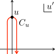
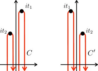
Figure 1: Left: Keldysh contour for the insertion of single operator. Right: Contours $C,C^{\prime}$ used in (3.4),(3.5).

As a result we obtain the following two real time equations from the continuation of (2.18)

$$-i\partial_{t_{1}}G_{ab}(it_{1}^{-},it_{2}^{+})-\sum_{c}\Bigl{(}-i\mu\epsilon_{ac}G_{cb}(it_{1}^{-},it_{2}^{+})+\int_{C}du^{\prime}\Sigma_{ac}(it_{1}^{-},u^{\prime})G_{cb}(u^{\prime},it_{2}^{+})\Bigr{)} =0,$$ (3.4)

$$-i\partial_{t_{1}}G_{ab}(it_{1}^{+},it_{2}^{-})-\sum_{c}\Bigl{(}-i\mu\epsilon_{ac}G_{cb}(it_{1}^{+},it_{2}^{-})+\int_{C^{\prime}}du^{\prime}\Sigma_{ac}(it_{1}^{+},u^{\prime})G_{cb}(u^{\prime},it_{2}^{-})\Bigr{)} =0,$$ (3.5)

where the integrations are over the contours depicted in Fig. 1 and can be rewritten as

$$\int_{C}du^{\prime}\Sigma_{ac}(it_{1}^{-},u^{\prime})G_{cb}(u^{\prime},it_{2}^{+}) =-i\int_{-\infty}^{\infty}dt_{3}(\Sigma_{ac}^{R}(t_{1},t_{3})G^{>}_{cb}(t_{3},t_{2})+\Sigma_{ac}^{>}(t_{1},t_{3})G^{A}_{cb}(t_{3},t_{2}))$$

$$\int_{C^{\prime}}du^{\prime}\Sigma_{ac}(it_{1}^{+},u^{\prime})G_{cb}(u^{\prime},it_{2}^{-}) =-i\int_{-\infty}^{\infty}dt_{3}(\Sigma_{ac}^{R}(t_{1},t_{3})G^{<}_{cb}(t_{3},t_{2})+\Sigma_{ac}^{<}(t_{1},t_{3})G^{A}_{cb}(t_{3},t_{2})).$$ (3.6)

Here we have defined the retarded/advanced component of the two point funcitons

$$G_{ab}^{R}(t_{1},t_{2}) =\theta(t_{1}-t_{2})(G^{>}(t_{1},t_{2})-G^{<}(t_{1},t_{2})),$$ (3.7)

$$G_{ab}^{A}(t_{1},t_{2}) =\theta(t_{2}-t_{1})(G^{<}(t_{1},t_{2})-G^{>}(t_{1},t_{2})),$$ (3.8)

and $\Sigma^{R}_{ab},\Sigma^{A}_{ab}$ in the same way. Taking the difference between (3.4) and (3.5), and using the formulas (3.6), we obtain

$$-i\partial_{t_{1}}G_{ab}^{R}(t_{1},t_{2})-\sum_{c}\Bigl{(}-i\mu\rho_{ac}G_{cb}^{R}(t_{1},t_{2})-\int dt_{3}(\Sigma_{ac}^{R}(t_{1},t_{3})G_{cb}^{R}(t_{3},t_{2})-\Sigma_{ac}^{A}(t_{1},t_{3})G_{cb}^{A}(t_{3},t_{2}))\Bigr{)}$$

$$\quad=-i\delta(t_{1}-t_{2})\cdot 2G^{>}_{ab}(t_{1},t_{1})=-\delta_{ab}\delta(t_{1}-t_{2}).$$ (3.9)

Here the second term in the integrand $\Sigma_{ac}^{A}(t_{1},t_{3})G_{cb}^{A}(t_{3},t_{2})$ vanishes for $t_{1}>t_{2}$, hence we end up with the following set of equations:

$$-i\partial_{t_{1}}G_{ab}^{R}(t_{1},t_{2})-\sum_{c}\Bigl{(}-i\mu\rho_{ac}G_{cb}^{R}(t_{1},t_{2})-\int dt_{3}\Sigma_{ac}^{R}(t_{1},t_{3})G_{cb}^{R}(t_{3},t_{2})\Bigr{)}=-\delta_{ab}\delta(t_{1}-t_{2}),$$ (3.10)

$$\Sigma_{ab}^{>}(t_{1},t_{2})=-\frac{i^{q}\mathcal{J}^{2}}{q}s_{ab}G^{>}_{ab}(t_{1},t_{2})^{q-1},$$ (3.11)

$$\Sigma_{ab}^{R}(t_{1},t_{2})=\theta(t_{1}-t_{2})(\Sigma_{ab}^{>}(t_{1},t_{2})+\Sigma_{ba}^{>}(t_{2},t_{1})).$$ (3.12)

Here we have also written the continuation of the second line of the equations of motion (2.16) and the definition of the retarded component (3.8) with $\Sigma_{ab}^{<}$ eliminated with the help of the anti-symmetric property $\Sigma_{ab}(u_{1},u_{2})=-\Sigma_{ba}(u_{2},u_{1})$ (2.17). If we assume $G_{ab}^{>}(t_{1},t_{2})$ and $G_{ab}^{R}(t_{1},t_{2})$ depends only on $t_{1}-t_{2}$, we can write the two point functions also in the Fourier modes

$${\widetilde{f}}^{X}(\omega)=\int_{-\infty}^{\infty}dte^{i\omega t}f^{X}(t),\quad f^{X}(t)=\int_{-\infty}^{\infty}\frac{d\omega}{2\pi}e^{-i\omega t}{\widetilde{f}}^{X}(t),\quad(f=G_{ab},\Sigma_{ab},\quad X=>,<,R,A).$$ (3.13)

The first equation (3.10) can be written in the Fourier modes as

$${\widetilde{G}}_{LL}^{R}(\omega)=\frac{-(-\omega+{\widetilde{\Sigma}}_{RR}^{R}(\omega))}{(-\omega+{\widetilde{\Sigma}}_{LL}^{R}(\omega))(-\omega+{\widetilde{\Sigma}}_{RR}^{R}(\omega))-({\widetilde{\Sigma}}_{LR}^{R}+i\mu)({\widetilde{\Sigma}}_{RL}^{R}-i\mu)},$$

$${\widetilde{G}}_{LR}^{R}(\omega)=\frac{{\widetilde{\Sigma}}_{LR}^{R}(\omega)+i\mu}{(-\omega+{\widetilde{\Sigma}}_{LL}^{R}(\omega))(-\omega+{\widetilde{\Sigma}}_{RR}^{R}(\omega))-({\widetilde{\Sigma}}_{LR}^{R}+i\mu)({\widetilde{\Sigma}}_{RL}^{R}-i\mu)},$$

$${\widetilde{G}}_{RL}^{R}(\omega)=\frac{{\widetilde{\Sigma}}_{RL}^{R}(\omega)-i\mu}{(-\omega+{\widetilde{\Sigma}}_{LL}^{R}(\omega))(-\omega+{\widetilde{\Sigma}}_{RR}^{R}(\omega))-({\widetilde{\Sigma}}_{LR}^{R}+i\mu)({\widetilde{\Sigma}}_{RL}^{R}-i\mu)},$$

$${\widetilde{G}}_{RR}^{R}(\omega)=\frac{-(-\omega+{\widetilde{\Sigma}}_{LL}^{R}(\omega))}{(-\omega+{\widetilde{\Sigma}}_{LL}^{R}(\omega))(-\omega+{\widetilde{\Sigma}}_{RR}^{R}(\omega))-({\widetilde{\Sigma}}_{LR}^{R}+i\mu)({\widetilde{\Sigma}}_{RL}^{R}-i\mu)}.$$ (3.14)

Apparently the equations (3.10)-(3.12), (3.14), and (3.8) are not closed by themselves as $G_{ab}^{R}$ does not completely determine $G_{ab}^{>}$ throught (3.8). This problem is fixed by taking into account the KMS condition (2.23) in the following way. First using the KMS relation in Lorentzian signature, we obtain

$$G_{ab}^{R}(t_{1},t_{2}) =\theta(t_{1}-t_{2})(G_{ab}^{>}(t_{1},t_{2})-G^{<}_{ab}(t_{1},t_{2}))$$

$$=\theta(t_{1}-t_{2})(G_{ab}^{>}(t_{1},t_{2})+G_{ab}^{>}(t_{1}-i\beta,t_{2})).$$ (3.15)

Next we consider $(G_{ba}^{R}(t_{2},t_{1}))^{*}$, use (2.22) to rewrite $(G_{ba}^{>,<})^{*}$ in terms of $G_{ab}^{>}$, and then do the same rewriting as above:

$$(G_{ba}^{R}(t_{2},t_{1}))^{*} =\theta(t_{2}-t_{1})(G^{>}_{ba}(t_{2},t_{1})^{*}-G^{<}_{ba}(t_{2},t_{1})^{*})$$

$$=\theta(t_{2}-t_{1})(G^{<}_{ba}(t_{2},t_{1})-G^{>}_{ba}(t_{2},t_{1}))$$

$$=\theta(t_{2}-t_{1})(-G^{>}_{ab}(t_{1},t_{2})+G^{<}_{ab}(t_{1},t_{2}))$$

$$=\theta(t_{2}-t_{1})(-G^{>}_{ab}(t_{1},t_{2})-G_{ab}^{>}(t_{1}-i\beta,t_{2})).$$ (3.16)

Combining these relations, we obtain

$$G_{ab}^{>}(t_{1},t_{2})+G_{ab}^{>}(t_{1}-i\beta,t_{2})=G_{ab}^{R}(t_{1},t_{2})-(G_{ba}^{R}(t_{2},t_{1}))^{*}.$$ (3.17)

In the Fourier modes this is written as

$${\widetilde{G}}_{ab}^{>}(\omega)=\frac{{\widetilde{G}}_{ab}^{R}(\omega)-({\widetilde{G}}_{ba}^{R}(\omega))^{*}}{1+e^{-\beta\omega}}.$$ (3.18)

Hence (3.10)-(3.12), (3.14) and (3.18) together form a closed system of the equations for $G_{ab}^{R}(t)$ which we can solve numerically.

Note that once we obtain the retarded component $G^{R}_{ab}(t)$, we can compute $G_{ab}(u)$ for general $u\in\mathbb{C}$ with $0<\text{Re}[u]<\beta$ as

$$G_{ab}(u)=iG_{ab}^{>}(t=-iu)=i\int\frac{d\omega}{2\pi}e^{-\omega u}\frac{{\widetilde{G}}_{ab}^{R}(\omega)-({\widetilde{G}}_{ba}^{R}(\omega))^{*}}{1+e^{-\beta\omega}},$$ (3.19)

which we use to compute the chaos exponent in section 3.1.4. Also note that by setting $u=\tau$ $(0<\tau<\beta)$ the formula (3.19) reproduces the Euclidean propagator which we can obtain relatively easily by solving the Schwinger-Dyson equations (2.18),(2.16) on the real contour, hence (3.19) can be also used as a trivial check for the validity of the real time computation.

3.1.2 Further symmetry ansatz

We can further impose the following symmetry properties consistently with the Schwinger-Dyson equations (3.10)-(3.12), (3.14) and the physical ansatz (2.22)-(2.23), (3.18)

$$G_{RR}^{>}(t)=G_{LL}^{>}(t),\quad G_{RL}^{>}(t)=-G_{LR}^{>}(t),\quad\Sigma_{RR}^{>}(t)=\Sigma_{LL}^{>}(t),\quad\Sigma_{RL}^{>}(t)=-\Sigma_{LR}^{>}(t).$$ (3.20)

Note that this corresponds to imposing the $\mathbb{Z}_{4}$ symmetry (2.5). Under these additional constraints, the Schwinger-Dyson equations (3.10)-(3.12), (3.14) reduce to the following set of equations:

$${\widetilde{G}}_{LL}^{R}(\omega) =\frac{-(-\omega+{\widetilde{\Sigma}}_{LL}^{R}(\omega))}{(-\omega+{\widetilde{\Sigma}}_{LL}^{R}(\omega))^{2}+({\widetilde{\Sigma}}_{LR}^{R}(\omega)+i\mu)^{2}},\quad{\widetilde{G}}_{LR}^{R}(\omega)=\frac{{\widetilde{\Sigma}}_{LR}^{R}(\omega)+i\mu}{(-\omega+{\widetilde{\Sigma}}_{LL}^{R}(\omega))^{2}+({\widetilde{\Sigma}}_{LR}^{R}(\omega)+i\mu)^{2}},$$

$$\Sigma_{LL}^{>}(t) =-\frac{i^{q}\mathcal{J}^{2}}{q}[2G_{LL}^{>}(t)]^{q-1},\quad\Sigma_{LR}^{>}(t)=-\frac{\mathcal{J}^{2}}{q}[2G_{LR}^{>}(t)]^{q-1},$$

$$\Sigma_{LL}^{R}(t) =\theta(t)(\Sigma_{LL}^{>}(t)+\Sigma_{LL}^{>}(-t)),\quad\Sigma_{LR}^{R}(t)=\theta(t)(\Sigma_{LR}^{>}(t)-\Sigma_{LR}^{>}(-t)),$$ (3.21)

while the constraints of the physical ansatz are now written as

$$G_{LL}^{>}(t)^{*} =-G_{LL}^{>}(-t),\quad G_{LR}^{>}(t)^{*}=G_{LR}^{>}(-t),$$

$${\widetilde{G}}_{LL}^{>}(\omega) =\frac{2i\text{Im}[{\widetilde{G}}_{LL}^{R}(\omega)]}{1+e^{-\beta\omega}}=-\frac{i\rho_{LL}(\omega)}{1+e^{-\beta\omega}},\quad{\widetilde{G}}_{LR}^{>}(\omega)=\frac{2\text{Re}[{\widetilde{G}}_{LR}^{R}(\omega)]}{1+e^{-\beta\omega}}=-\frac{\rho_{LR}(\omega)}{1+e^{-\beta\omega}}.$$ (3.22)

Here we have defined the spectral functions

$$\rho_{LL}(\omega)=-2\text{Im}[{\widetilde{G}}_{LL}^{R}(\omega)],\quad\rho_{LR}(\omega)=-2\text{Re}[{\widetilde{G}}_{LR}^{R}(\omega)].$$ (3.23)

As we see in section 4, these quantities are useful to characterize the gapped regime.

3.1.3 Four point function

We consider the following four point function which is written as the two point function in the $G\Sigma$ formalism:

$$\frac{1}{(N/2)^{2}}\sum_{i,j}^{N/2}\langle\psi_{i}^{a}(u_{1})\psi_{i}^{b}(u_{2})\psi_{j}^{c}(u_{3})\psi_{j}^{d}(u_{4})\rangle=\frac{1}{Z_{\text{two}}}\int{\cal D}G_{ab}{\cal D}\Sigma_{ab}G_{ab}(u_{1},u_{2})G_{cd}(u_{1},u_{2})e^{-NS_{\text{two}}}.$$ (3.24)

In the large $N$ limit we can evaluate this correlation function by expanding $S_{\text{two}}$ around a solution of the Schwinger-Dyson equations (2.15),(2.16), $G_{ab}=G_{ab}^{(0)}+N^{-\frac{1}{2}}\delta G_{ab}$, $\Sigma_{ab}=\Sigma_{ab}^{(0)}+N^{-\frac{1}{2}}\delta\Sigma_{ab}$ as

$$S_{\text{two}} =S_{\text{two}}^{(0)}+\sum_{a,b,c,d}\frac{1}{8N}\int du_{1}du_{2}du_{3}du_{4}$$

$$\quad\begin{pmatrix}-\delta(u-u^{\prime})\partial_{u^{\prime}}+\frac{\Sigma_{LL}^{(0)}(u,u^{\prime})-\Sigma_{LL}^{(0)}(u^{\prime},u)}{2}&\frac{\Sigma_{LR}^{(0)}(u,u^{\prime})-\Sigma_{RL}^{(0)}(u^{\prime},u)}{2}-i\mu\delta(u-u^{\prime})\\ \frac{\Sigma_{RL}^{(0)}(u,u^{\prime})-\Sigma_{LR}^{(0)}(u^{\prime},u)}{2}+i\mu\delta(u-u^{\prime})&-\delta(u-u^{\prime})\partial_{u^{\prime}}+\frac{\Sigma_{RR}^{(0)}(u,u^{\prime})-\Sigma_{RR}^{(0)}(u^{\prime},u)}{2}\end{pmatrix}^{-1}_{da}(u_{4},u_{1})$$

$$\quad\frac{\delta\Sigma_{ab}(u_{1},u_{2})-\delta\Sigma_{ba}(u_{2},u_{1})}{2}$$

$$\quad\begin{pmatrix}-\delta(u-u^{\prime})\partial_{u^{\prime}}+\frac{\Sigma_{LL}^{(0)}(u,u^{\prime})-\Sigma_{LL}^{(0)}(u^{\prime},u)}{2}&\frac{\Sigma_{LR}^{(0)}(u,u^{\prime})-\Sigma_{RL}^{(0)}(u^{\prime},u)}{2}-i\mu\delta(u-u^{\prime})\\ \frac{\Sigma_{RL}^{(0)}(u,u^{\prime})-\Sigma_{LR}^{(0)}(u^{\prime},u)}{2}+i\mu\delta(u-u^{\prime})&-\delta(u-u^{\prime})\partial_{u^{\prime}}+\frac{\Sigma_{RR}^{(0)}(u,u^{\prime})-\Sigma_{RR}^{(0)}(u^{\prime},u)}{2}\end{pmatrix}^{-1}_{bc}(u_{2},u_{3})$$

$$\quad\frac{\delta\Sigma_{cd}(u_{3},u_{4})-\delta\Sigma_{dc}(u_{4},u_{3})}{2}$$

$$\quad+\sum_{a,b}\frac{1}{4N}\int du_{1}du_{2}$$

$$\quad\Bigl{(}\delta\Sigma_{ab}(u_{1},u_{2})\delta G_{ab}(u_{1},u_{2})-\frac{\mathcal{J}^{2}2^{q-1}(q-1)}{2q}s_{ab}G^{(0)}_{ab}(u_{1},u_{2})^{q-2}\delta G_{ab}(u_{1},u_{2})^{2}\Bigr{)}$$ (3.25)

where the terms of ${\cal O}(\delta G_{ab},\delta\Sigma_{ab})$ trivially vanish since we are expanding $G_{ab},\Sigma_{ab}$ around a solution of the equations of motion. Note that the matrix elements in the first term can be replaced with $-G_{da}(u_{4},u_{1})$ and $-G_{bc}(u_{2},u_{3})$ with the help of (2.15). Also noticing that $G_{ab}^{(0)}(u,u^{\prime})=-G_{ba}^{(0)}(u^{\prime},u)$, we obtain

$$S_{\text{two}} =S^{(0)}_{\text{two}}+\sum_{a,b,c,d}\frac{1}{8N}\int du_{1}du_{2}du_{3}du_{4}\frac{G_{ac}^{(0)}(u_{1},u_{3})G_{bd}^{(0)}(u_{2},u_{4})-G_{ad}^{(0)}(u_{1},u_{4})G_{bc}^{(0)}(u_{2},u_{3})}{2}$$

$$\quad\delta\Sigma_{ab}(u_{1},u_{2})\delta\Sigma_{cd}(u_{3},u_{4})+\sum_{a,b}\frac{1}{4N}\int du_{1}du_{2}$$

$$\quad\Bigl{(}\delta\Sigma_{ab}(u_{1},u_{2})\delta G_{ab}(u_{1},u_{2})-\frac{\mathcal{J}^{2}2^{q-1}(q-1)}{2q}s_{ab}G^{(0)}_{ab}(u_{1},u_{2})^{q-2}\delta G_{ab}(u_{1},u_{2})^{2}\Bigr{)}$$

$$=S_{\text{two}}^{(0)}+\sum_{A,B}\frac{1}{8N}\int dUdV{\cal G}_{AB}(U,V)\delta\Sigma_{A}(U)\delta\Sigma_{B}(V)$$

$$\quad+\sum_{A}\frac{1}{4N}\Bigl{(}\delta\Sigma_{A}(U)\delta G_{A}(U)-\frac{\mathcal{J}^{2}2^{q-1}(q-1)}{2q}s_{A}G_{A}^{(0)}(U)^{q-2}\delta G_{A}(U)^{2}\Bigr{)},$$ (3.26)

where in the second line we have abbreviated the pair of indices/coordinates as $A=(a,b)$, $U=(u_{1},u_{2})$, and denoted the kernel of $\delta\Sigma$ as ${\cal G}_{A}(U,V)$:

$${\cal G}_{AB}(U,V)=\frac{G^{(0)}_{A_{1}B_{1}}(U_{1},V_{1})G^{(0)}_{A_{2}B_{2}}(U_{2},V_{2})-G^{(0)}_{A_{1}B_{2}}(U_{1},V_{2})G^{(0)}_{A_{2}B_{1}}(U_{2},V_{1})}{2}.$$ (3.27)

Since the inserted operator $G_{ab}(u_{1},u_{2})G_{cd}(u_{3},u_{4})$ does not depends on $\Sigma_{ab}$ we can integrate $\delta\Sigma_{ab}$ first, which is under the current approximation simply a Gaussian integration:

$$\int{\cal D}\Sigma_{ab}e^{-NS_{\text{two}}}$$

$$=e^{-S_{\text{two}}^{(0)}}\int{\cal D}\delta\Sigma_{A}\exp\biggl{[}-\sum_{A,B}\frac{1}{8}\int dUdV{\cal G}_{AB}(U,V)\delta\Sigma_{A}(U)\delta\Sigma_{B}(V)$$

$$\quad-\frac{1}{4}\sum_{A}\int dU\Bigl{(}\delta G_{A}(U)\delta\Sigma_{A}(U)-\frac{\mathcal{J}^{2}2^{q-1}(q-1)}{2q}G_{A}^{(0)}(U)^{q-2}\delta G_{A}(U)^{2}\Bigr{)}\biggr{]}$$

$$=e^{-S_{\text{two}}^{(0)}}\int{\cal D}\delta\Sigma_{A}\exp\biggl{[}-\frac{1}{8}\sum_{A,B}\int dUdV\Bigl{(}\delta\Sigma_{A}(U)-\sum_{C}\int dW\delta G_{C}(W)({\cal G}^{-1})_{CA}(W,U)\Bigr{)}$$

$$\quad{\cal G}_{AB}(U,V)\Bigl{(}\delta\Sigma_{B}(V)-\sum_{D}\int dX({\cal G}^{-1})_{BD}(V,X)\delta G_{D}(X)\Bigr{)}$$

$$\quad+\sum_{A,B}\int dUdV\delta G_{A}(U)\Bigl{(}\frac{1}{8}({\cal G}^{-1})_{AB}(U,V)$$

$$\quad+\frac{\mathcal{J}^{2}2^{q-1}(q-1)}{8q}s_{A}G_{A}^{(0)}(U)^{q-2}\delta_{AB}\delta(U-V)\Bigr{)}\delta G_{B}(V)\biggr{]}$$

$$=e^{-S_{\text{two}}^{(0)}}\exp\biggl{[}-\frac{1}{8}\sum_{A,B}\int dUdV\delta G_{A}(U)\Bigl{(}({\cal G}^{-1})_{AB}(U,V)$$

$$\quad+\frac{\mathcal{J}^{2}2^{q-1}(q-1)}{q}s_{A}G_{A}^{(0)}(U)^{q-2}\delta_{AB}\delta(U-V)\Bigr{)}\delta G_{B}(V)\biggr{]}.$$ (3.28)

Expanding the inserted $G_{ab}(u_{1},u_{2})G_{cd}(u_{3},u_{4})$ also around the saddle configuration, now we are left with the Gaussian integration in $\delta G_{A}(U)$ which we can perform as

$$\frac{1}{(N/2)^{2}}\sum_{i,j}^{N/2}\langle\psi_{i}^{a}(u_{1})\psi_{i}^{b}(u_{2})\psi_{j}^{c}(u_{3})\psi_{j}^{d}(u_{4})\rangle=G^{(0)}_{ab}(u_{1},u_{2})G^{(0)}_{cd}(u_{3},u_{4})+\frac{1}{(N/2)}{\cal F}_{abcd}(u_{1},u_{2},u_{3},u_{4})$$ (3.29)

Swiching the notation back to $A\rightarrow(a,b)$, $U\rightarrow(u_{1},u_{2})$, the connected part ${\cal F}_{abcd}(u_{1},u_{2},u_{3},u_{4})$ of the four point function is written as

$${\cal F}_{abcd}(u_{1},u_{2},u_{3},u_{4})$$

$$=-2\Bigl{[}({\cal G}^{-1})_{AB}(U,V)$$

$$\quad+\frac{\mathcal{J}^{2}2^{q-1}(q-1)}{q}s_{A}G_{A}^{(0)}(U)^{q-2}\delta_{AB}\delta(U-V)\Bigr{]}^{-1}_{A=(a,b),B=(c,d)}(U=(u_{1},u_{2}),V=(u_{3},u_{4}))$$

$$=\sum_{n=0}^{\infty}{\cal F}_{n,abcd}(u_{1},u_{2},u_{3},u_{4}).$$ (3.30)

with

$${\cal F}_{0,abcd}(u_{1},u_{2},u_{3},u_{4})=-2{\cal G}_{(a,b),(c,d)}((u_{1},u_{2}),(v_{1},v_{2}))$$

$$\quad\quad\quad\quad\quad\quad\quad\quad\quad=-G^{(0)}_{ac}(u_{1},u_{3})G^{(0)}_{bd}(u_{2},u_{4})+G_{ad}^{(0)}(u_{1},u_{4})G_{bc}^{(0)}(u_{2},u_{3}),$$

$${\cal F}_{n,abcd}(u_{1},u_{2},u_{3},u_{4})$$

$$=\sum_{B}\int dV\biggl{[}-{\cal G}_{(a,b),B}((u_{1},u_{2}),V)\cdot\frac{\mathcal{J}^{2}2^{q-1}(q-1)}{q}s_{B}G_{B}^{(0)}(V)^{q-1}\biggr{]}_{(a,b),B}((u_{1},u_{2}),V)$$

$$\quad\quad\quad\quad{\cal F}_{n,B_{1}B_{2}cd}(V_{1},V_{2},u_{3},u_{4})$$

$$=\sum_{e,f}\int dvdv^{\prime}{\cal K}_{abef}(u_{1},u_{2},v,v^{\prime}){\cal F}_{n-1,efcd}(v,v^{\prime},u_{3},u_{4}),$$

$${\cal K}_{abcd}(u_{1},u_{2},u_{3},u_{4})=-\frac{\mathcal{J}^{2}2^{q-1}(q-1)}{q}G^{(0)}_{ac}(u_{1},u_{3})G^{(0)}_{bd}(u_{2},u_{4})s_{cd}G^{(0)}_{cd}(u_{3},u_{4})^{q-2}.$$ (3.31)

Here to write down the ladder kernel ${\cal K}_{abcd}(u_{1},u_{2},u_{3},u_{4})$ we have used the fact that the matrix on which ${\cal K}$ acts, ${\cal F}_{n,abcd}(u_{1},u_{2},u_{3},u_{4})$, is always anti-symmetric under $(a,u_{1})\leftrightarrow(b,u_{2})$, which holds inductively. Note that ${\cal F}_{abcd}$ obeys the following self consistency equation

$${\cal F}_{abcd}(u_{1},u_{2},u_{3},u_{4})={\cal F}_{0,abcd}(u_{1},u_{2},u_{3},u_{4})+\sum_{e,f}\int dvdv^{\prime}{\cal K}_{abef}(u_{1},u_{2},v,v^{\prime}){\cal F}_{efcd}(v,v^{\prime},u_{3},u_{4}),$$ (3.32)

which we use in the next section.

3.1.4 Chaos exponent from OTOC at late time

Now we continue $u_{1},u_{2},u_{3},u_{4}$ in (3.32) to

$$u_{1}=\frac{3\beta}{4}+it_{1},\quad u_{2}=\frac{\beta}{4}+it_{2},\quad u_{3}=\frac{\beta}{2},\quad u_{4}=0,$$ (3.33)

and take the integration contour of $v,v^{\prime}$ as the following Keldysh contour.

We are interested in the growing behavior of ${\cal F}(3\beta/4+it_{1},\beta/4+it_{2},\beta/2,0)\equiv{\cal F}(t_{1},t_{2})$ at late time $t_{1},t_{2}\gg 1$, where the only relevant contributions in the right-hand side of (3.32) are the second terms with $v\in C_{u_{1}},v^{\prime}\in C_{u_{2}}$; the integrations with $v\in C_{u_{2}}$ or $v^{\prime}\in C_{u_{1}}$ cancel by themselves due to the regularity of the integrand, and all the other terms including the first term ${\cal F}_{0,abcd}$ in (3.32) are suppressed as they contain the two point functions evaluated at $u$ with $\text{Im}[u]\sim t_{1},t_{2}$ being large. For the same reason, since the integration over $v\in C_{u_{1}}$, $v^{\prime}\in C_{u_{2}}$ is dominated only by the contributions from $\text{Im}[v_{1}]\sim t_{1},\text{Im}[v_{2}]\sim t_{2}$, we can freely add to $C_{u_{1}}$ and $C_{u_{2}}$ the infinite intervals $\text{Im}[v],\text{Im}[v^{\prime}]\in(-\infty,0)$. Hence we can approximate the ladder relation (3.32) as

$${\cal F}_{abcd}(t_{1},t_{2}) \approx\sum_{ef}\int dtdt^{\prime}{\cal K}^{R}_{abef}(t_{1},t_{2},t,t^{\prime}){\cal F}_{efcd}(t,t^{\prime}),$$

$${\cal K}^{R}_{abcd}(t_{1},t_{2},t_{3},t_{4}) =-\frac{\mathcal{J}^{2}2^{q-1}(q-1)}{q}G_{ac}^{(0)R}(t_{1}-t_{3})G_{bd}^{(0)R}(t_{2}-t_{4})s_{cd}G_{cd}^{(0)}\Bigl{(}\frac{\beta}{2}+i(t_{3}-t_{4})\Bigr{)}^{q-2}.$$ (3.34)

If we further pose the following ansatz

$${\cal F}_{abcd}(t_{1},t_{2})=e^{\frac{\lambda_{L}(t_{1}+t_{2})}{2}}f_{abcd}(t_{12}),$$ (3.35)

we finally obtain, after a little change of the integration variables,

$$f_{abcd}(t_{12}) \approx-\frac{\mathcal{J}^{2}2^{q-1}(q-1)}{q}\sum_{ef}\int dt_{-}e^{-\frac{\lambda_{L}(t_{12}-t_{-})}{2}}\biggl{[}\int dt^{\prime\prime}G_{ae}^{(0)R}(t_{12}-t_{-}-t^{\prime\prime})G_{bf}^{(0)R}(-t^{\prime\prime})e^{\lambda_{L}t^{\prime\prime}}\biggr{]}$$

$$\quad s_{ef}G_{ef}^{(0)}\Bigl{(}\frac{\beta}{2}+it_{-}\Bigr{)}^{q-2}f_{efcd}(t_{-}),$$ (3.36)

The consequences of this equation are the followings. First suppose that $\lambda_{L}$ is less than or equal to the actual value of the largest chaos exponent of the system. Then the mode (3.35) indeed exists and hence (3.36) has a non-trivial solution $f(t)$ corresponding to that mode. On the other hand, if $\lambda_{L}$ is larger than the largest chaos exponent, such mode does not exist and hence (3.36) can only have a trivial solution $f(t)=0$. Regarding the operation in the right-hand side of (3.36) as a matrix, the former case is possible only if the largest eigenvalue of the matrix is greater than or equal to $1$. Therefore we can obtain the chaos exponent by varying the test value $\lambda_{L}$ and finding the point where the largest eigenvalue crosses $1$. This procedure can be implemented numerically by the power iteration method.

We cau further simplify the ladder equation (3.36) as follows. First of all, notice that the indices $cd$ of $f_{2,abcd}$ are not mixed through the operation of $M_{1},M_{2}$. This implies that we have only to consider a single choice of $cd$, say $cd=LL$, which hereafter we do not write: $f_{ab}\equiv f_{abLL}$. Next, using the symmetry properties $G^{>}_{LL}(t)=G^{>}_{RR}(t)$, $G^{>}_{LR}(t)=-G_{RL}^{>}(t)$ we have imposed by hand (3.20), we can show that the kernel ${\cal K}_{abcd}^{R}(t_{1},t_{2},t_{3},t_{4})$ (3.34) is invariant under the simultaneous replacement $L\leftrightarrow R$ in the four indices $abcd$ together with a sign multiplication

$${\cal K}^{R}_{IJ}\rightarrow\begin{pmatrix}0&0&0&1\\ 0&0&-1&0\\ 0&-1&0&0\\ 1&0&0&0\end{pmatrix}_{IK}{\cal K}^{R}_{KL}\begin{pmatrix}0&0&0&1\\ 0&0&-1&0\\ 0&-1&0&0\\ 1&0&0&0\end{pmatrix}_{LJ},\quad\quad(I=LL,LR,RL,LL)$$ (3.37)

which is equivalent to the following change of basis of ${\cal F}_{ab}$:

$$\begin{pmatrix}{\cal F}_{LL}\\ {\cal F}_{LR}\\ {\cal F}_{RL}\\ {\cal F}_{RR}\end{pmatrix}\rightarrow\begin{pmatrix}0&0&0&1\\ 0&0&-1&0\\ 0&-1&0&0\\ 1&0&0&0\end{pmatrix}\begin{pmatrix}{\cal F}_{LL}\\ {\cal F}_{LR}\\ {\cal F}_{RL}\\ {\cal F}_{RR}\end{pmatrix}.$$ (3.38)

Hence the ladder equation splits to the one for the ${\cal F}_{ab}$ which is symmetric under the flip: $({\cal F}_{LL},{\cal F}_{LR},{\cal F}_{RL},{\cal F}_{RR})=({\cal F}_{LL},{\cal F}_{LR},-{\cal F}_{LR},{\cal F}_{LL})$ and the one for ${\cal F}_{ab}$ being antisymmetric: $({\cal F}_{LL},{\cal F}_{LR},{\cal F}_{RL},{\cal F}_{RR})=({\cal F}_{LL},{\cal F}_{LR},{\cal F}_{LR},-{\cal F}_{LL})$. We can finally write the ladder equation for the symmetric/anti-symmetric sector, which we denote by $\sigma=\pm 1$, as

$$\begin{pmatrix}f_{2,LL}+\sigma f_{2,RR}\\ f_{2,LR}-\sigma f_{2,RL}\end{pmatrix}$$

$$=\begin{pmatrix}M_{1,LLLL}+\sigma M_{1,LRLR}&M_{1,LLLR}-\sigma M_{1,LRLL}\\ -(M_{1,LLLR}-\sigma M_{1,LRLL})&M_{1,LLLL}+\sigma M_{1,LRLR}\end{pmatrix}\circ\begin{pmatrix}M_{2,LL}(f_{2,LL}+\sigma f_{2,RR})\\ M_{2,LR}(f_{2,LR}-\sigma f_{2,RL})\end{pmatrix}$$ (3.39)

where $\circ$ is the convolution $(f\circ g)(t)=\int dt^{\prime}f(t-t^{\prime})g(t^{\prime})$ and

$$f_{2,ab}(t_{12}) =e^{\frac{\lambda_{L}t_{12}}{2}}f_{ab}(t_{12}),$$

$$M_{1,abcd}(t) =\int dt^{\prime}G_{ab}^{(0)R}(t-t^{\prime})G^{(0)R}_{cd}(-t^{\prime})e^{\lambda_{L}t^{\prime}},$$

$$M_{2,ab}(t) =-\frac{\mathcal{J}^{2}2^{q-1}(q-1)}{q}s_{ab}G_{ab}^{(0)}\Bigl{(}\frac{\beta}{2}+it\Bigr{)}^{q-2}.$$ (3.40)

Note that $M_{1,abcd}$ itself can also be written as a convolution: $M_{1,abcd}=G^{(0)R}_{ab}\circ({\widehat{G}}^{(0)R}_{cd}e^{\lambda_{L}t})$ with ${\widehat{G}}^{(0)R}_{ab}(t)=G^{(0)}_{ab}(-t)$.

3.2 Single sided model

3.2.1 Real time Schwinger-Dyson equation

Thanks to the redundant $G\Sigma$ formalism (2.25),(2.26), the calculation for the single sided model is completely parallel to those for the two coupled model; the only difference is in the form of the potential term of $G_{ab}(u,u^{\prime})$ (right-hand side of (2.28)), which do not disturb the argument on the analytic continuation in sectoin 3.1.1,3.1.4 and the derivation of the ladder equation in section 3.1.3. Hence we obtain the following set of real time Schwinger-Dyson equations

$$-i\partial_{t_{1}}G_{LL}^{R}(t_{1},t_{2})+i\mu G_{RL}^{R}(t_{1},t_{2})+\int dt_{3}\Sigma_{LL}^{R}(t_{1},t_{3})G_{LL}^{R}(t_{3},t_{2})=-\delta(t_{1}-t_{2}),$$

$$-i\partial_{t_{1}}G_{LR}^{R}(t_{1},t_{2})+i\mu G_{RR}^{R}(t_{1},t_{2})+\int dt_{3}\Sigma_{LL}^{R}(t_{1},t_{3})G_{LR}^{R}(t_{3},t_{2})=0,$$

$$-i\partial_{t_{1}}G_{RL}^{R}(t_{1},t_{2})-i\mu G_{LL}^{R}(t_{1},t_{2})+\int dt_{3}\Sigma_{LL}^{R}(t_{1},t_{3})G_{RL}^{R}(t_{3},t_{2})=0,$$

$$-i\partial_{t_{1}}G_{RR}^{R}(t_{1},t_{2})-i\mu G_{LR}^{R}(t_{1},t_{2})+\int dt_{3}\Sigma_{LL}^{R}(t_{1},t_{3})G_{RR}^{R}(t_{3},t_{2})=-\delta(t_{1}-t_{2}),$$ (3.41)

$$\Sigma_{LL}^{>}(t_{1},t_{2})=-\frac{i^{q}\mathcal{J}^{2}}{q}\Bigl{(}G^{>}_{LL}(t_{1},t_{2})+G^{>}_{RR}(t_{1},t_{2})\Bigr{)}^{q-1},$$ (3.42)

$$\Sigma_{LL}^{R}(t_{1},t_{2})=\theta(t_{1}-t_{2})(\Sigma_{LL}^{>}(t_{1},t_{2})+\Sigma_{LL}^{>}(t_{2},t_{1})),$$ (3.43)

where we have also used the fact $\Sigma_{RR}(u,u^{\prime})=\Sigma_{LL}(u,u^{\prime})$ and $\Sigma_{LR}(u,u^{\prime})=\Sigma_{RL}(u^{\prime},u)=0$ (2.29). If we assume that $G_{ab}^{>}(t_{1},t_{2})$ and $G_{ab}^{R}(t_{1},t_{2})$ depend only on $t_{1}-t_{2}$, we obtain from the first four equations (3.41)

$${\widetilde{G}}_{LL}^{R}(\omega)={\widetilde{G}}_{RR}^{R}(\omega)=\frac{-(-\omega+{\widetilde{\Sigma}}_{LL}^{R}(\omega))}{(-\omega+{\widetilde{\Sigma}}_{LL}^{R}(\omega))^{2}-\mu^{2}},$$ (3.44)

$${\widetilde{G}}_{LR}^{R}(\omega)=-{\widetilde{G}}_{RL}^{R}(\omega)=\frac{i\mu}{(-\omega+{\widetilde{\Sigma}}_{LL}^{R}(\omega))^{2}-\mu^{2}},$$ (3.45)

The greater components $G^{>}_{ab}(t)$ are related to the retarded components as

$${\widetilde{G}}_{ab}^{>}(\omega)=\frac{{\widetilde{G}}_{ab}^{R}(\omega)-({\widetilde{G}}_{ba}^{R}(\omega))^{*}}{1+e^{-\beta\omega}},$$ (3.46)

or explicitly

$${\widetilde{G}}_{LL}^{>}(\omega)=\frac{2i\text{Im}[{\widetilde{G}}_{LL}^{R}(\omega)]}{1+e^{-\beta\omega}}=-\frac{i\rho_{LL}(\omega)}{1+e^{-\beta\omega}},\quad{\widetilde{G}}_{LR}^{>}(\omega)=\frac{2\text{Re}[{\widetilde{G}}_{LR}^{R}(\omega)]}{1+e^{-\beta\omega}}=-\frac{\rho_{LR}(\omega)}{1+e^{-\beta\omega}},$$ (3.47)

where we have defined the spectral functions $\rho_{LL}(\omega)=-2\text{Im}[{\widetilde{G}}_{LL}(\omega)]$, $\rho_{LR}(\omega)=-2\text{Re}[{\widetilde{G}}_{LR}(\omega)]$ in the same was as in the two coupled model (3.23). As we have already mentioned at the end of section 2.1.2, the Schwinger-Dyson equations are decomposed into a closed set of equations only for $G_{LL}^{R}$, $G_{LL}^{>}$, $\Sigma_{LL}^{R}$, $\Sigma_{LL}^{>}$ (3.42),(3.43),(3.44),(3.47) and the rest which gives $G_{LR}^{R}$, $G_{LR}^{>}$ explicitly in terms of $\Sigma_{LL}^{R}$ (3.45),(3.47).

Once we obtain the retarded component $G^{R}_{ab}(t)$, we can compute $G_{ab}(u)$ for general $u\in\mathbb{C}$ with $0<\text{Re}[u]<\beta$ as

$$G_{ab}(u)=iG_{ab}^{>}(t=-iu)=i\int\frac{d\omega}{2\pi}e^{-\omega u}\frac{{\widetilde{G}}_{ab}^{R}(\omega)-({\widetilde{G}}_{ba}^{R}(\omega))^{*}}{1+e^{-\beta\omega}},$$ (3.48)

and $G_{ab}(u)$ with $-\beta<\text{Re}[u]<0$ by using the anti-symmetry property $G_{ab}(u)=-G_{ba}(-u)$ (2.29).

3.2.2 Four point function

The caculation for the four point functions is also in parallel. If we denote $\chi_{2i-1}(u)$ as $\chi_{i}^{L}(u)$ and $\chi_{2i}(u)$ as $\chi_{i}^{R}(u)$, the four point functions are expressed in the large $N$ limit as follows

$$\frac{1}{(N/2)^{2}}\sum_{i,j}^{\frac{N}{2}}\langle\chi_{i}^{a}(u_{1})\chi_{i}^{b}(u_{2})\chi_{j}^{c}(u_{3})\chi_{j}^{d}(u_{4})\rangle =\frac{1}{Z_{\text{single}}}\int{\cal D}G_{ab}{\cal D}\Sigma_{ab}G_{ab}(u_{1},u_{2})G_{cd}(u_{3},u_{4})e^{-NS_{\text{single}}}$$

$$=G_{ab}^{(0)}(u_{1},u_{2})G_{cd}^{(0)}(u_{3},u_{4})+\frac{1}{(N/2)}{\cal F}_{abcd}(u_{1},u_{2},u_{3},u_{4})$$ (3.49)

where $G_{ab}^{(0)}$ are a solutions to the Schwinger-Dyson equations. The connected part ${\cal F}_{abcd}$ is

$${\cal F}_{abcd}(u_{1},u_{2},u_{3},u_{4})=\sum_{n=0}^{\infty}{\cal F}_{n,abcd}(u_{1},u_{2},u_{3},u_{4})$$ (3.50)

where

$${\cal F}_{0,abcd}(u_{1},u_{2},u_{3},u_{4})=-G_{ac}^{(0)}(u_{1},u_{3})G_{bd}^{(0)}(u_{2},u_{4})+G_{ad}^{(0)}(u_{1},u_{4})G_{bc}^{(0)}(u_{2},u_{3}),$$

$${\cal F}_{n,abcd}(u_{1},u_{2},u_{3},u_{4})=\sum_{e,f}\int dvdv^{\prime}{\cal K}_{abef}^{\text{(single)}}(u_{1},u_{2},v,v^{\prime}){\cal F}_{n-1,abcd}(v,v^{\prime},u_{3},u_{4}),$$ (3.51)

with

$${\cal K}_{abcd}^{\text{(single)}}(u_{1},u_{2},u_{3},u_{4}) =-\frac{\mathcal{J}^{2}2^{q-1}(q-1)}{2q}\Bigl{(}\sum_{e}G_{ae}^{(0)}(u_{1},u_{3})G_{be}^{(0)}(u_{2},u_{4})\Bigr{)}$$

$$\quad\Bigl{(}\frac{G_{LL}^{(0)}(u_{3},u_{4})+G_{RR}^{(0)}(u_{3},u_{4})}{2}\Bigr{)}^{q-2}\delta_{cd}.$$ (3.52)

Here we observe an additional simplification which did not occur in the two coupled model: due to the structure of the $cd$ index in ${\cal K}_{abcd}^{\text{(single)}}$ it follows that the recursive relation (3.52) decomposes to the following recursive relation which closes only within ${\cal F}_{ab}(u_{1},u_{2},u_{3},u_{4})\equiv{\cal F}_{LLab}(u_{1},u_{2},u_{3},u_{4})+{\cal F}_{RRab}(u_{1},u_{2},u_{3},u_{4})$

$${\cal F}_{n,ab}(u_{1},u_{2},u_{3},u_{4}) =\int dvdv^{\prime}{\cal K}^{\text{(single)}}(u_{1},u_{2},v,v^{\prime}){\cal F}_{n-1,ab}(v,v^{\prime},u_{3},u_{4}),$$

$${\cal K}^{\text{(single)}}(u_{1},u_{2},u_{3},u_{4}) =-\frac{\mathcal{J}^{2}2^{q-1}(q-1)}{2q}\Bigl{(}\sum_{a,b}G_{ab}^{(0)}(u_{1},u_{3})G_{ab}^{(0)}(u_{2},u_{4})\Bigr{)}$$

$$\quad\Bigl{(}\frac{G_{LL}^{(0)}(u_{3},u_{4})+G_{RR}^{(0)}(u_{3},u_{4})}{2}\Bigr{)}^{q-2},$$ (3.53)

and the rest which explicitly determines the other components of ${\cal F}_{abcd}(u_{1},u_{2},u_{3},u_{4})$ in terms of ${\cal F}_{cd}(u_{1},u_{2},u_{3},u_{4})$:

$${\cal F}_{n,abcd}(u_{1},u_{2},u_{3},u_{4}) =-\frac{\mathcal{J}^{2}2^{q-1}(q-1)}{2q}\int dvdv^{\prime}\Bigl{(}\sum_{e}G_{ae}^{(0)}(u_{1},u_{3})G_{be}^{(0)}(u_{2},u_{4})\Bigr{)}$$

$$\quad\Bigl{(}\frac{G_{LL}^{(0)}(u_{3},u_{4})+G_{RR}^{(0)}(u_{3},u_{4})}{2}\Bigr{)}^{q-2}{\cal F}_{n-1,cd}(v,v^{\prime},u_{3},u_{4}).$$ (3.54)

Therefore, for the purpose of determining the chaos exponent of the single sided model, it is enough to proceed with only the recursive relation for ${\cal F}_{ab}(u_{1},u_{2},u_{3},u_{4})$ written in the form of a self-consistency equation

$${\cal F}_{ab}(u_{1},u_{2},u_{3},u_{4})={\cal F}_{0,ab}(u_{1},u_{2},u_{3},u_{4})+\int dvdv^{\prime}{\cal K}^{\text{(single)}}(u_{1},u_{2},v,v^{\prime}){\cal F}_{ab}(v,v^{\prime},u_{3},u_{4}).$$ (3.55)

where ${\cal F}_{0,ab}(u_{1},u_{2},u_{3},u_{4})={\cal F}_{0,LLab}(u_{1},u_{2},u_{3},u_{4})+{\cal F}_{0,RRab}(u_{1},u_{2},u_{3},u_{4})$.

3.2.3 Chaos exponent

By continuing the ladder equation (3.55) to real time with $u_{1}=3\beta/4+it_{1}$, $u_{2}=\beta/4+it_{2}$, $u_{3}=\beta/2$, $u_{4}=0$ and assuming a growing behavior of ${\cal F}_{ab}(t_{1},t_{2})\equiv{\cal F}_{ab}(3\beta/4+it_{1},\beta/4+it_{2},\beta/2,0)$ at late time $t_{1},t_{2}\gg 1$, we obtain the following real time ladder equation

$${\cal F}_{ab}(t_{1},t_{2}) \approx\int dtdt^{\prime}{\cal K}^{\text{(single)}R}(t_{1},t_{2},t,t^{\prime}){\cal F}_{ab}(t,t^{\prime}),$$ (3.56)

with the retarded kernel given as

$${\cal K}^{\text{(single)}R}(t_{1},t_{2},t_{3},t_{4})$$

$$=-\frac{\mathcal{J}^{2}2^{q-1}(q-1)}{2q}\Bigl{(}\sum_{a,b}G_{ab}^{(0)R}(t_{1}-t_{3})G_{ab}^{(0)R}(t_{2}-t_{4})\Bigr{)}$$

$$\quad\Bigl{(}\frac{G_{LL}^{(0)}(\frac{\beta}{2}+i(t_{3}-t_{4}))+G_{RR}^{(0)}(\frac{\beta}{2}+i(t_{3}-t_{4}))}{2}\Bigr{)}^{q-2}$$

$$=-\frac{\mathcal{J}^{2}2^{q-1}(q-1)}{q}(G_{LL}^{(0)R}(t_{1}-t_{3})G_{LL}^{(0)R}(t_{2}-t_{4})+G_{LR}^{(0)R}(t_{1}-t_{3})G_{LR}^{(0)R}(t_{2}-t_{4}))G_{LL}^{(0)}$$

$$\quad\Bigl{(}\frac{\beta}{2}+i(t_{3}-t_{4})\Bigr{)}^{q-2},$$ (3.57)

where in the third line we have used the fact that $G^{(0)R}_{RL}(t)=-G^{(0)R}_{LR}(t)$ and $G^{(0)}_{RR}(u)=G^{(0)}_{LL}(u)$ (3.44),(3.45). If we further pose the exponentially growing ansatz

$${\cal F}_{ab}(t_{1},t_{2})=e^{\frac{\lambda_{L}(t_{1}+t_{2})}{2}}f_{ab}(t_{12}),$$ (3.58)

the real time ladder equation reduces to

$$f_{ab}(t_{12}) \approx-\frac{\mathcal{J}^{2}2^{q-1}(q-1)}{q}\int dt_{-}e^{-\frac{\lambda_{L}(t_{12}-t_{-})}{2}}\biggl{[}\int dt^{\prime\prime}(G_{LL}^{(0)R}(t_{12}-t_{-}-t^{\prime\prime})G_{LL}^{(0)R}(-t^{\prime\prime})$$

$$\quad+G_{LR}^{(0)R}(t_{12}-t_{-}-t^{\prime\prime})G_{LR}^{(0)R}(-t^{\prime\prime}))e^{\lambda_{L}t^{\prime\prime}}\biggr{]}G_{LL}^{(0)}\Bigl{(}\frac{\beta}{2}+it_{-}\Bigr{)}^{q-2}f_{ab}(t_{-}).$$ (3.59)

We can also understand the structure of the retarded kernels and ladder equations using diagrams (figure 2).

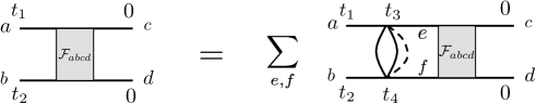
Figure 2: Top/Middle: The diagrammatic representation of the ladder equation/ retarded kernel (3.34). Bottom: The diagrammatic representation of the retarded kernel (3.57).

4 Results

In this section we display the numerical results for the real time two point functions and the chaos exponent of the two coupled model and the single sided model. In all of the following analyses we have chosen $q=4$ and ${\cal J}=1$ for both of the two models. Some results for different values of $q$ are displayed in appendix A.

4.1 Two coupled model

4.1.1 Euclidean propagator $G_{ab}(\tau)$, phase diagram and $E_{\text{gap}}$

When the contour of $u$ in (2.6) is taken as the Euclidean slice $u=\tau\in(0,\beta)$ with $\tau\sim\tau+\beta$, the partition function gives the thermal free energy

$$\frac{F(T)}{N}=-\frac{1}{\beta N}\log Z\approx-\frac{1}{\beta N}\sum_{\text{saddles}}e^{-NS_{\text{two}}[G_{ab}^{\text{(saddle)}},\Sigma_{ab}^{\text{(saddle)}}]},\quad\quad T=\beta^{-1},$$ (4.1)

where $(G_{ab}^{\text{(saddle)}},\Sigma_{ab}^{\text{(saddle)}})$ are the solutions of the Schwinger-Dyson equations (2.18),(2.16).

By solving the Schwinger-Dyson equations numerically by using the iteration method [7] we found that when $\mu$ is smaller than $\mu_{c}\approx 0.177$ [31], for each $\mu$ there are two distinctive solutions each of which varies continuously as the temperature is varied. One of these two solutions exists only for $T>T_{c,\text{BH}}$ while the other exists only for $T<T_{c,\text{WH}}$ with some $T_{c,\text{BH}}(\mu),T_{c,\text{WH}}(\mu)$ which satisfies $T_{c,\text{BH}}<T_{c,\text{WH}}$. For example for $\mu=0.1$ we have obtained $T_{c,\text{BH}}=0.032$, $T_{c,\text{WH}}=0.04$. We call the solution exists at high temperature “the black hole (BH) solution” and the other “the wormhole (WH) solution”. See Fig. 3 for the profile of these two solutions.

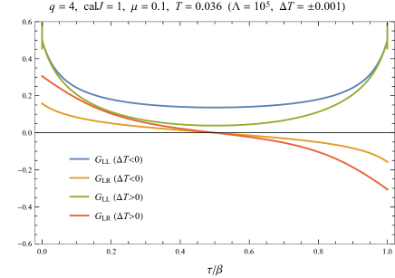
Figure 3: Euclidean propagators for the black hole phase ($\Delta T<0$) and those for the wormhole phase ($\Delta T>0$).

The free energies evaluated at these two solution intersect at some $T_{c}(\mu)$ which satisfies $T_{c,\text{BH}}<T_{c}<T_{c,\text{WH}}$ hence the system exhibhts a first order phase transition at $T=T_{c}$. See Fig. 4 for the phase diagram together with the list of $T_{c,\text{BH}}$ and $T_{c,\text{WH}}$.

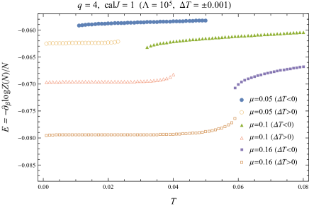
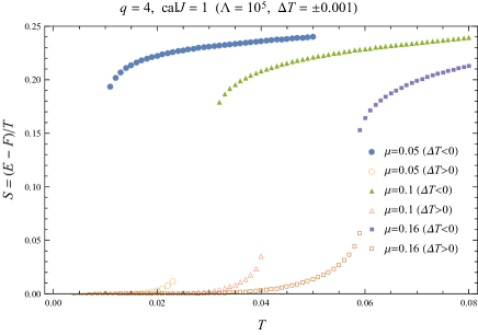
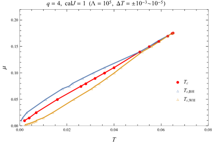
Figure 4: Top left/top right/bottom left: free energy/energy/entropy for the black hole solution and the wormhole solution; bottom right: phase diagram of the two coupled model. In the phase diagram we have computed $T_{c,\text{BH}}$, $T_{c}$ and $T_{c,\text{WH}}$ for $\mu=0.07,0.08,0.09,0.1$ and $\mu\geq 0.16$ with $\Delta T=\pm 10^{-5}$, $T_{c,\text{BH}}$ for $\mu=0.01,0.015$ and $T_{c,\text{WH}}$ for $0.002\leq\mu\leq 0.009$ with $\Delta T=\pm 10^{-4}$, while all the other data points with $\Delta T=10^{-3}$.

Note that the values of $T_{c,\text{BH}}$ and $T_{c,\text{WH}}$ we have obtained are respectively higher and lower compared with those displayed in [23, 39]. These discrepancies are presumably because our criterion for a given configuration to be the solution (4.2) is more strict than that adopted in [39]. We have further evidence for the values of $T_{c,\text{BH}}$ and $T_{c,\text{WH}}$: (i) for several values of $\mu$ we ran the iterations with $\Delta T=\pm 0.0001$ as well as $\Delta T=\pm 0.001$, and obtained the same values of $(T_{c,\text{BH}},T_{c,\text{WH}})$; (ii) we have obtained the same values of $T_{c,\text{BH}},T_{c,\text{WH}}$ from the numerical study of the real time Schwinger-Dyson equation. However, at present it is not clear which results are closer to the exact values of $T_{c,\text{BH}}$, $T_{c,\text{WH}}$.

We observe that the slope of the energy $E(T)$ diverges as the temperature approaches $T_{c,\text{BH}}$ in the black hole phase or $T_{c,\text{WH}}$ in the wormhole phase, where we can define the critical exponents $\nu_{\text{BH}}$, $\nu_{\text{WH}}$ as

$$c_{T}=\frac{\partial E}{\partial T}\sim\begin{cases}(T-T_{c,\text{BH}})^{-\nu_{\text{BH}}}\quad(T\approx T_{c,\text{BH}},\,\text{black hole phase})\\ (T_{c,\text{WH}}-T)^{-\nu_{\text{WH}}}\quad(T\approx T_{c,\text{WH}},\,\text{wormhole phase})\end{cases}.$$ (4.3)

We have obtained $\nu_{\text{BH}},\nu_{\text{WH}}\approx 0.5$ when $\mu$ is not close to $\mu_{c}$, while $\nu_{\text{BH}},\nu_{\text{WH}}$ approaches $\approx 0.66$ as $\mu$ approaches $\mu_{c}$. See Fig. 5.

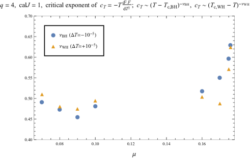
Figure 5: The critical exponents $\nu_{\text{BH}}$, $\nu_{\text{WH}}$ of the specific heat (4.3) of the two coupled model with $q=4$, ${\cal J}=1$. We have determined $\nu_{\text{BH}}$, $\nu_{\text{WH}}$ by fitting $(\partial E/\partial T)^{-1}$ near the discontinuity of $E(T)$ (Fig. 4) by the ansatz $(\partial E/\partial T)^{-1}=c(T-T_{c,\text{BH}})^{\nu_{\text{BH}}}$ and $(\partial E/\partial T)^{-1}=c(T_{c,\text{WH}}-T)^{\nu_{\text{WH}}}$ with the fitting parameters $(c,\nu_{\text{BH}})$ and $(c,\nu_{\text{WH}})$.

These results are consistent with the claim that there are no phase transition in the micro canonical picture [23], where the black hole phase and the wormhole phase are smoothly connected by a canonically unstable intermediate phase which was called “hot wormhole phase” in [39]. Indeed, if $T(E)$ is infinitely differentiable with respect to $E$ at the canonical critical points $E_{c,\text{BH}}\equiv E(T_{c,\text{WH}})$ and $E_{c,\text{WH}}\equiv E(T_{c,\text{WH}})$, we have $T(E)=T_{c,\text{BH}}+(\cdots)(E-E_{c,\text{BH}})^{m}+\cdots$ and $T(E)=T_{c,\text{WH}}+(\cdots)(E_{c,\text{WH}}-E)^{n}+\cdots$ around these points, with $m,n$ being some integers greater than $1$. Inverting these relations we find that the possible values of critical exponents are $1-1/\mathbb{N}_{>1}=1/2,2/3,\cdots$. The critical exponents we found for $\mu<\mu_{c}$ and for $\mu\rightarrow\mu_{c}$ are close to $1/2$ and $2/3$ respectively.

As we can see from Fig. 6 (left), the wormhole solution exhibits exponential decay $G_{ab}(\tau)\sim e^{-E_{\text{gap}}\tau}$ which indicates that the system is gapped with the energy gap $E_{\text{gap}}$. Indeed when the temperature is sufficiently low ($\beta$ is large) the two point functions can be expanded as

$$\langle\psi^{a}_{i}(\tau)\psi_{i}^{b}(0)\rangle_{\beta} =\frac{1}{Z(\beta)}\text{Tr}e^{\tau{\widehat{H}}}{\widehat{\psi}}^{a}_{i}e^{-\tau{\widehat{H}}}{\widehat{\psi}}_{i}^{b}e^{-\beta{\widehat{H}}}$$

$$=\frac{1}{Z(\beta)}\sum_{m,n}\langle E_{m}|{\widehat{\psi}}_{i}^{a}|E_{n}\rangle\langle E_{n}|{\widehat{\psi}}_{i}^{b}|E_{m}\rangle e^{-\beta E_{m}+\tau(E_{m}-E_{n})}$$

$$\approx\langle E_{0}|{\widehat{\psi}}_{i}^{a}|E_{0}\rangle\langle E_{0}|{\widehat{\psi}}_{i}^{b}|E_{0}\rangle+\langle E_{0}|{\widehat{\psi}}_{i}^{a}|E_{1}\rangle\langle E_{1}|{\widehat{\psi}}_{i}^{b}|E_{0}\rangle e^{-(E_{1}-E_{0})\tau}+\cdots,$$ (4.4)

where the fist term is zero since the Hamiltonian of the two coupled model preserves parity (fermion number) symmetry. See Fig. 6 (right) for the values of $E_{\text{gap}}(\mu)$ which we have obtained by fitting the Euclidean propagators at $T=0.001$.

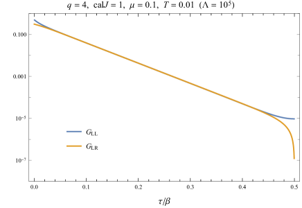
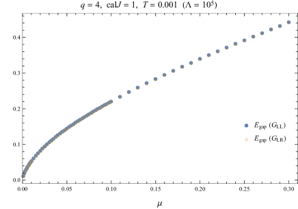
Figure 6: Left: Euclidean propagator for the wormhole phase around $\tau\sim 0$ which show exponential decay $G_{ab}(\tau)\sim e^{-E_{\text{gap}}\tau}$ with a common exponent $E_{\text{gap}}$ for $ab=LL,LR$. Right: $E_{\text{gap}}$ obtained by fitting $G_{ab}(\tau)$ of the wormhole solutions at $T=0.001$.

For $\mu>\mu_{c}$ there is only one solution with which both the BH/WH solutions in the subcritical regime are smoothly connected.

4.1.2 Real time propagator $G_{ab}^{>}(t)$ and decay rates $\Gamma$

By solving the real time Schwinger-Dyson equations (3.21),(3.22) we found two distinctive solutions for each single point on the $\mu$-$T$ plane around the line $T=T_{c}(\mu)$ (see Fig. 7). These two solutions correspond respectively to the black hole phase and the wormhole phase. Indeed, by calculating the Euclidean propagator from the spectral function of each solution by (3.19), we have obtained precisely the same configuration as those obtained by directly solving the Euclidean Schwinger-Dyson equations. We have also found that the real time BH/WH solution stops to exist precisely at $T=T_{c,\text{BH}}$/$T=T_{c,\text{WH}}$ as we decrease/increase the temperature slowly, as we have mentioned in the previous subsection. In Fig. 7 we have displayed the real time propagator $G_{ab}^{>}(t)$ together with the spectral functions $\rho_{LL}(\omega)=-2\text{Im}[{\widetilde{G}}_{LL}(\omega)]$, $\rho_{LR}(\omega)=-2\text{Re}[{\widetilde{G}}_{LR}(\omega)]$ of BH/WH phase for $\mu=0.1$, $T=0.036$. Note that these two quantities $(G_{ab}^{>}(t),\rho_{ab}(\omega))$ are not independent with each other; given one of them one can construct the other through (3.8),(3.22).

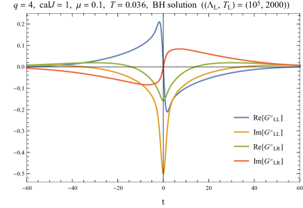
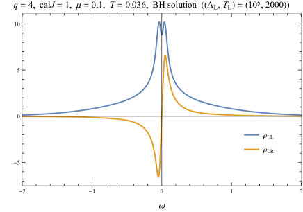
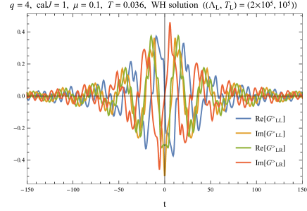
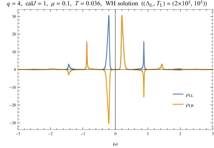
Figure 7: Top left/right: propagators/spectral functions $\rho_{LL}(\omega)=-2\text{Im}[{\widetilde{G}}^{R}_{LL}(\omega)]$, $\rho_{LR}(\omega)=-2\text{Re}[{\widetilde{G}}^{R}_{LR}(\omega)]$ for the black hope solution. Bottom left/right: propagators/spectral functions for the wormhole solution.

Here are additional remarks on the wormhole solution. As shown in Fig. 7, the spectral functions $\rho_{ab}(\omega)$ of the wormhole solution split into sharp peaks. We find that the position of the peaks are same for $\rho_{LL}(\omega)$ and $\rho_{LR}(\omega)$ and, in particular, the position of the first peak is in good agreement with $E_{\text{gap}}$ obtained by fitting the Euclidean propagator (see Fig. 6). Indeed, if $\rho_{ab}(\omega)$ were given as $\rho_{LL}(\omega)=A_{LL}(\delta(\omega-E_{\text{gap}})+\delta(\omega+E_{\text{gap}}))$ and $\rho_{LR}(\omega)=A_{LR}(\delta(\omega-E_{\text{gap}})-\delta(\omega+E_{\text{gap}}))$, then from (3.19) we obtain

$$G_{LL}(\tau) =\frac{A_{LL}}{\pi}\Bigl{(}\frac{e^{-E_{\text{gap}}\tau}}{1+e^{-\beta E_{\text{gap}}}}+\frac{e^{E_{\text{gap}}\tau}}{1+e^{\beta E_{\text{gap}}}}\Bigr{)}\approx\frac{A_{LL}}{\pi}e^{-E_{\text{gap}}\tau},$$

$$G_{LR}(\tau) =-\frac{iA_{LR}}{\pi}\Bigl{(}\frac{e^{-E_{\text{gap}}\tau}}{1+e^{-\beta E_{\text{gap}}}}-\frac{e^{E_{\text{gap}}\tau}}{1+e^{\beta E_{\text{gap}}}}\Bigr{)}\approx-\frac{iA_{LR}}{\pi}e^{-E_{\text{gap}}\tau}.$$ (4.5)

The situation is not completely same with the actual result of $\rho_{ab}$ where there are infinitely many other peaks and each peak is of finite width. Each peak can be fit well with $A\delta_{\Gamma}(\omega-\omega_{0})$ with $\delta_{\Gamma}(\omega)=-\frac{1}{\pi}\text{Im}[\frac{1}{\omega-\omega_{0}+i\Gamma}]$ (see Fig. 8), which corresponds to a particle of finite lifetime:

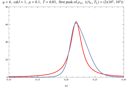
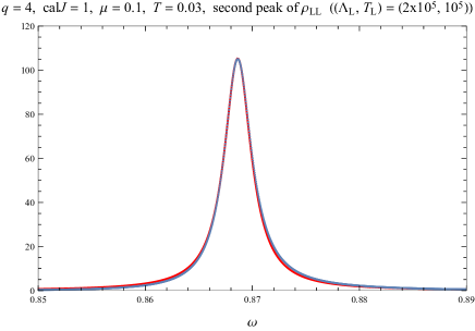
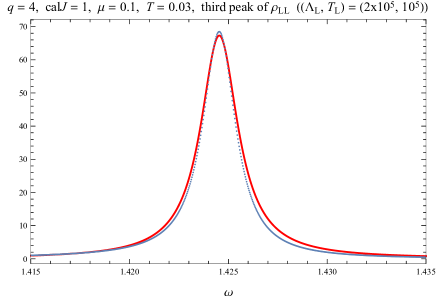
	$\omega_{0}$	$A$	$\Gamma$
$LL$, 1st	$0.217$	$2.28$	$0.0115$
$LL$, 2nd	$0.869$	$0.508$	$0.00153$
$LL$, 3rd	$1.42$	$0.243$	$0.00115$
$LR$, 1st	$0.217$	$2.28$	$0.0115$
$LR$, 2nd	$0.869$	$0.508$	$0.00153$
$LR$, 3rd	$1.42$	$0.242$	$0.00114$

Figure 8: Top left/top right/bottom left: first/second/third peak of the spectral function $\rho_{LL}(\omega)$ for $q=4$, ${\cal J}=1$, $\mu=0.1$, $T=0.03$ with $(\Lambda_{L},T_{L})=(2\times 10^{5},10^{5})$. Red lines: fitting curve $\frac{A}{\pi}\frac{\Gamma}{(\omega-\omega_{0})^{2}+\Gamma^{2}}$. Here we have determined $A,\omega_{0}$ separately as the integration of $\rho_{LL}$ around the peak and the local maximim, and used only $\Gamma$ as the fitting parameter. Bottom right: results of fitting for the first three peaks of $\rho_{LL}(\omega)$, $\rho_{LR}(\omega)$.

$$\rho_{LL}(\omega)=A_{LL}(\delta_{\Gamma}(\omega-E_{\text{gap}})+\delta_{\Gamma}(\omega+E_{\text{gap}}))$$

$$\quad\Rightarrow\quad G^{>}_{LL}=-\frac{iA_{LL}}{\pi}\Bigl{(}\frac{e^{-iE_{\text{gap}}t}}{1+e^{-\beta E_{\text{gap}}}}+\frac{e^{iE_{\text{gap}}t}}{1+e^{\beta E_{\text{gap}}}}\Bigr{)}e^{-\Gamma|t|},$$

$$\rho_{LR}(\omega)=A_{LR}(\delta_{\Gamma}(\omega-E_{\text{gap}})-\delta_{\Gamma}(\omega+E_{\text{gap}}))$$

$$\quad\Rightarrow\quad G^{>}_{LR}=-\frac{A_{LR}}{\pi}\Bigl{(}\frac{e^{-iE_{\text{gap}}t}}{1+e^{-\beta E_{\text{gap}}}}-\frac{e^{iE_{\text{gap}}t}}{1+e^{\beta E_{\text{gap}}}}\Bigr{)}e^{-\Gamma|t|}.$$ (4.6)

The decay width of each peak decreases as the temperature decreases. In order the finite IR cutoff $|t|<T_{L}/2$ to be a good approximation to the reality $t\in(-\infty,\infty)$, $T_{L}$ has to be sufficiently larger than the inverse of the decay rates so that $G_{ab}^{R}(t),G_{ab}^{>}(t)\approx 0$ at the IR cutoff and the effect of compactification $t\sim t+t_{L}$ is negligible. For example, for $\mu=0.1$, if we choose $\Lambda_{L},T_{L}$ as $\Lambda_{L}=10^{5}$, $T_{L}=2000$ we could solve the Schwinger-Dyson equation only for $T\geq 0.03$. In general when we increase $T_{L}$ we also have to increase the number of the discrete points $\Lambda_{L}$ at the same rate to keep the UV resolution, which makes the numerics at low temperature difficult. However, we found that the weight of the peak $A$ is smaller for the higher peaks. In particular, for $\mu=0.1$, $T=0.03$ the total weight of the first three peaks of $\rho_{LL}$ is $6.04$, which is $96.1\%$ of the total weight $\int d\omega\rho_{LL}(\omega)=2\pi i(G_{LL}^{R}(+0)-(G_{LL}^{R}(-0))^{*})=2\pi$; $\rho_{LL}$ is well approximated by the contributions of only first three peaks. We found this is the case also for other values of $\mu,T$ as long as the temperature is low enough so that the peaks are well separated. This fact implies that the sufficient value of $\Lambda_{L}$ relative to $T_{L}$ is such that $\omega_{\text{max}}=(\pi/T_{L})(\Lambda_{L}-1/2)$ is larger than the position of the third peak. This required value is much smaller than $\omega_{\text{max}}=157$ for $(\Lambda_{L},T_{L})=(10^{5},2000)$, hence we can improve the numerics at low temperature by just increasing $T_{L}$ with $\Lambda_{L}$ kept the same. Indeed, by choosing $(\Lambda_{L},T_{L})=(2\times 10^{5},10^{5})$, for $\mu=0.1$ we achieved to reach down to $T=0.019$.

We have displayed in Fig. 8 the fitting results for the first three peaks of the wormhole solution at $\mu=0.1$, $T=0.03$. The results we have obtained are consistent with those displayed in [1, 35]. We have also found that the decay rate of the first peak $\Gamma_{\text{1st}}$ obeys the following relation with $E_{\text{gap}}$

$$\Gamma_{\text{1st}}\sim e^{-\frac{1}{2}E_{\text{gap}}\beta}$$ (4.7)

up to some overall constant which is independent of $T$, as argued in [1]. See Fig. 9.

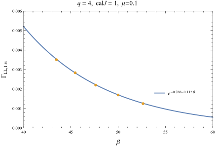
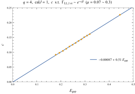
Figure 9: Left: Fitting of decay width of the first peak of $\rho_{LL}$ $\Gamma_{LL,\text{1st}}$ for $\mu=0.1$ with $e^{c_{1}-c_{2}\beta}$. Right: Comparison of the fitting coefficient $c_{2}$ with $E_{\text{gap}}$.

Interestingly, we have found that the chaos exponent $\lambda_{L}$ also obeys the same formula in the wormhole phase, as we display in the next subsection.

4.1.3 Chaos exponent

We can compute the chaos exponent of the two coupled model by solving the ladder equation (3.36) with the ladder kernel evaluated on the real time propagators obtained in the previous section. As we have seen in (3.39), the ladder equation decomposes into the two sectors which are even/odd under the $L\leftrightarrow R$ flipping (3.38), hence we can compute the chaos exponent for each sector separately. We have observed that the chaos exponent of the even ($\sigma=+1$) sector is always larger than that of the odd ($\sigma=-1$) sector (see Fig. 10), hence below we focus on the even sector.

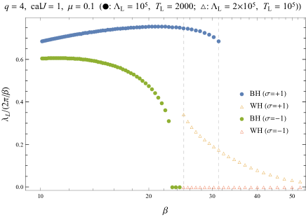
Figure 10: Chaos exponent of the two coupled model with $q=4$, ${\cal J}=1$, $\mu=0.1$ computed separately for $L\leftrightarrow R$ even/odd sector ($\sigma=\pm 1$).

In Fig. 11 we have displayed the chaos exponent of the even sector for various $\mu$ in the two phases.

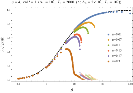
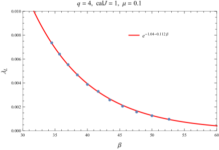
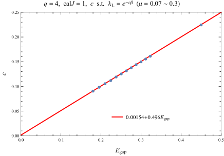
Figure 11: Top left: chaos exponent for the black hole solution and the wormhole solution, where the dashed black line is the chaos exponent of the pure SYK model $\mu=0$. Top right: Fitting of the chaos exponent for $\mu=0.1$ with $e^{c_{1}-c_{2}\beta}$. Bottom: Comparison of the fitting coefficient $c_{2}$ with $E_{\text{gap}}$.

It is remarkable that the chaos exponent is small but non-zero even in the wormhole phase. This is indeed consistent with the fact that the decay rate is small but non-zero in the same phase, as we have seen in the previous subsection; the system thermalize, which is another indication for the system to be quantum chaotic. Furthermore, we have found that the chaos exponent obeys completely the same formula (4.7) as the decay rate of the first peak when the temperature is low enough

$$\lambda_{L}\sim e^{-\frac{1}{2}\beta E_{\text{gap}}},$$ (4.8)

up to an overall factor which is independent of $T$. See Fig. 11. We have found this formula is also satisfied for $\mu>\mu_{c}$ where there are no phase transition, if the temperature is sufficiently low, as was the case also for $\Gamma_{\text{1st}}$.

We also observe that the slope of the chaos exponent of the black hole phase $\partial\lambda_{L}/\partial T$ diverges as the temperature approaches $T_{c,\text{BH}}$ (Fig. 12).

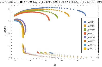
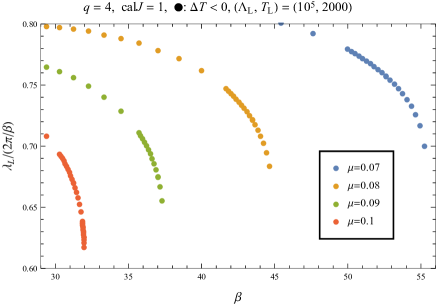
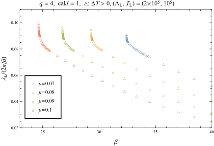
Figure 12: The chaos exponent of the two coupled model near $T=T_{c,\text{BH}}$ and $T=T_{c,\text{WH}}$ ($q=4$, ${\cal J}=1$). The data point in the black hole phase are generated with $(\Lambda_{L},T_{L})=(10^{5},2000)$ and $\Delta T=-10^{-3},-10^{-4},-10^{-5}$, while the data points in the wormhole phase are generated with $(\Lambda_{L},T_{L})=(2\times 10^{5},10^{5})$ and $\Delta T=10^{3},10^{4},10^{5}$.

Similarly, the slope also seems to diverge in the wormhole phase at $T=T_{c,\text{WH}}$. From the detailed analysis close to $T=T_{c,\text{BH}}$ and $T=T_{c,\text{WH}}$ we have identified the critical exponent as

$$\frac{\partial\lambda_{L}}{\partial T}\sim\begin{cases}&(T-T_{c,\text{BH}})^{\eta_{\text{BH}}}\quad(T\approx T_{c,\text{BH}},\,\text{black hole phase})\\ &(T_{c,\text{WH}}-T)^{\eta_{\text{WH}}}\quad(T\approx T_{c,\text{WH}},\,\text{wormhole phase})\end{cases}$$ (4.9)

with $\eta_{\text{BH}}$ and $\eta_{\text{WH}}$ displayed in Fig. 13.

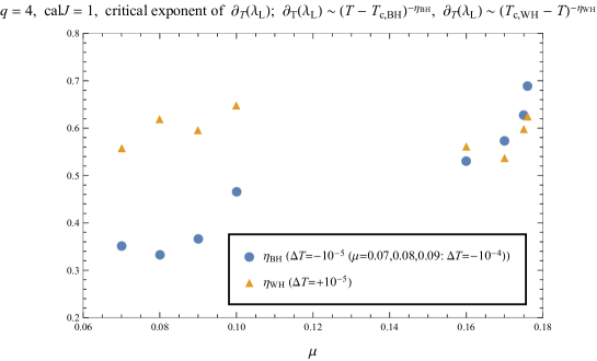
Figure 13: The critical exponent $\eta_{\text{BH}}$ and $\eta_{\text{WH}}$ of the chaos exponent (4.9) of the two coupled model with $q=4$, ${\cal J}=1$. We have determined $\eta_{\text{BH}}$, $\eta_{\text{WH}}$ by fitting $(\partial_{T}\lambda_{L})^{-1}$ by the ansatz $(\partial_{T}\lambda_{L})^{-1}=c(T-T_{c,\text{BH}})^{\eta_{\text{BH}}}$ and $(\partial_{T}\lambda_{L})^{-1}=c(T_{c,\text{WH}}-T)^{\eta_{\text{WH}}}$ with the fitting parameters $(c,\eta_{\text{BH}})$ and $(c,\eta_{\text{WH}})$.

In particular, as $\mu$ approaches $\mu_{c}=0.177$ the two critical exponents almost coincide around $\eta\approx 2/3$. This agrees with the behavior of the critical exponent $\nu_{\text{BH}},\nu_{\text{WH}}$ defined by the specific heat (4.3), and is consistent with the fact that for $\mu\geq\mu_{c}$ the phase transition disappears and the two phases are smoothly connected. On the other hand, for $\mu\leq 0.1$ the critical exponents deviate significantly from those of the specific heat $\nu_{\text{BH}},\nu_{\text{WH}}\approx 1/2$, except $\eta_{\text{BH}}(\mu=0.1)$ and $\eta_{\text{WH}}(\mu=0.07)$.

4.1.4 Chaos exponent in quasi-particle approximation

In the wormhole phase at $T\ll T_{\text{WH}}$, we can reduce the ladder equation (3.34), which is originally a set of integral equations, to a simple differential equation. This enables us to evaluate the chaos exponent in this regime analytically in terms of $E_{\text{gap}}$ and the decay rate of the first peak $\Gamma$.

The calculation goes as follows. When the temperature is sufficiently low, the spectral function is dominated by the first peak and its mirror image

$$\rho_{LL}(\omega)\approx\pi(\delta_{\Gamma}(\omega-E_{\text{gap}})+\delta_{\Gamma}(\omega+E_{\text{gap}})),\quad\rho_{LR}(\omega)\approx\pi(\delta_{\Gamma}(\omega-E_{\text{gap}})-\delta_{\Gamma}(\omega+E_{\text{gap}})),$$ (4.10)

from which we obtain, via (3.22),

$$G_{LL}^{R}(t) \approx-\frac{i}{2}\theta(t)(e^{-iE_{\text{gap}}t}+e^{iE_{\text{gap}}t})e^{-\Gamma t},\quad G_{LL}\Bigl{(}\frac{\beta}{2}+it\Bigr{)}\approx e^{-\frac{\beta E_{\text{gap}}}{2}}\cos(E_{\text{gap}}t)e^{-\Gamma|t|},$$

$$G_{LR}^{R}(t) \approx-\frac{1}{2}\theta(t)(e^{-iE_{\text{gap}}t}-e^{iE_{\text{gap}}t})e^{-\Gamma t},\quad G_{LR}\Bigl{(}\frac{\beta}{2}+it\Bigr{)}\approx-e^{-\frac{\beta E_{\text{gap}}}{2}}\sin(E_{\text{gap}}t)e^{-\Gamma|t|}.$$ (4.11)

By substituting these $G_{LL}^{R}$, $G_{LR}^{R}$ into the ladder equation (3.34) we obtain, under the assumption ${\cal F}_{RL}=-{\cal F}_{LR}$, ${\cal F}_{RR}={\cal F}_{LL}$ (here we suppress the last two indices of ${\cal F}_{abcd}$ to which the ladder kernel does not act, and we denote ${\cal F}_{abcd}$ simply as ${\cal F}_{ab}$), the following equations

$${\cal F}_{LL}(t_{1},t_{2})\pm i{\cal F}_{LR}(t_{1},t_{2})$$

$$=\frac{{\cal J}^{2}\cdot 2^{q-1}(q-1)}{q}\int dtdt^{\prime}\theta(t_{1}-t)\theta(t_{2}-t^{\prime})e^{(\mp iE_{\text{gap}}-\Gamma)(t_{1}-t)}e^{(\pm iE_{\text{gap}}-\Gamma)(t_{2}-t^{\prime})}$$

$$\quad\Bigl{[}G_{LL}\Bigl{(}\frac{\beta}{2}+i(t-t^{\prime})\Bigr{)}^{q-2}{\cal F}_{LL}(t,t^{\prime})\pm i(-1)^{\frac{q}{2}}G_{LR}\Bigl{(}\frac{\beta}{2}+i(t-t^{\prime})\Bigr{)}^{q-2}{\cal F}_{LR}(t,t^{\prime})\Bigr{]}.$$ (4.12)

Now we differentiate both sides of this equation by $\partial_{t_{1}}+\Gamma\pm iE_{\text{gap}}$ and $\partial_{t_{2}}+\Gamma\mp iE_{\text{gap}}$. Since the exponential factors in (4.12) are eliminated by these differential operators, from the right-hand side of (4.12) only gain $\partial_{t_{1}}\partial_{t_{2}}\theta(t_{1}-t)\theta(t_{2}-t^{\prime})=\delta(t_{1}-t)\delta(t_{2}-t^{\prime})$, which cancel the integrations and we obtain a differential equation

$$(\partial_{t_{1}}+\Gamma\pm iE_{\text{gap}})(\partial_{t_{2}}+\Gamma\mp iE_{\text{gap}})({\cal F}_{LL}(t_{1},t_{2})\pm i{\cal F}_{LR}(t_{1},t_{2}))=\frac{{\cal J}^{2}\cdot 2^{q-1}(q-1)}{q}$$

$$\quad\Bigl{[}G_{LL}\Bigl{(}\frac{\beta}{2}+i(t_{1}-t_{2})\Bigr{)}^{q-2}{\cal F}_{LL}(t_{1},t_{2})\pm i(-1)^{\frac{q}{2}}G_{LR}\Bigl{(}\frac{\beta}{2}+i(t_{1}-t_{2})\Bigr{)}^{q-2}{\cal F}_{LR}(t_{1},t_{2})\Bigr{]}.$$ (4.13)

If we assume the $t_{1}+t_{2}$ dependence of ${\cal F}_{ab}(t_{1},t_{2})$ as ${\cal F}_{ab}=e^{\lambda_{L}(t_{1}+t_{2})/2}f_{ab}(t_{1}-t_{2})$ and also assume $f_{ab}\in\mathbb{R}$, the ladder equation (4.13) becomes ($t\equiv t_{1}-t_{2}$)

$$\Bigl{[}-\partial_{t}^{2}+E_{\text{gap}}^{2}+\Bigl{(}\frac{\lambda_{L}}{2}+\Gamma\Bigr{)}^{2}\Bigr{]}f_{LL}(t)+2E_{\text{gap}}\partial_{t}f_{LR}(t)$$

$$\quad=\frac{{\cal J}^{2}\cdot 2^{q-1}(q-1)}{q}G_{LL}\Bigl{(}\frac{\beta}{2}+it\Bigr{)}^{q-2}f_{LL}(t),$$

$$\Bigl{[}-\partial_{t}^{2}+E_{\text{gap}}^{2}+\Bigl{(}\frac{\lambda_{L}}{2}+\Gamma\Bigr{)}^{2}\Bigr{]}f_{LR}(t)-2E_{\text{gap}}\partial_{t}f_{LL}(t)$$

$$\quad=\frac{(-1)^{\frac{q}{2}}{\cal J}^{2}\cdot 2^{q-1}(q-1)}{q}G_{LR}\Bigl{(}\frac{\beta}{2}+it\Bigr{)}^{q-2}f_{LR}(t),$$ (4.14)

For $q\in 4\mathbb{N}$ these equations simplify drastically with the following additional ansatz

$$f_{LL}(t)=\cos(E_{\text{gap}}t)g(t),\quad f_{LR}(t)=-\sin(E_{\text{gap}}t)g(t),$$ (4.15)

as

$$\Bigl{[}-\partial_{t}^{2}+\Bigl{(}\frac{\lambda_{L}}{2}+\Gamma\Bigr{)}^{2}\Bigr{]}g(t) =\frac{{\cal J}^{2}\cdot 2^{q-1}(q-1)}{q}G_{LL}\Bigr{(}\frac{\beta}{2}+it\Bigr{)}^{q-2}g(t),$$

$$\Bigl{[}-\partial_{t}^{2}+\Bigl{(}\frac{\lambda_{L}}{2}+\Gamma\Bigr{)}^{2}\Bigr{]}g(t) =\frac{{\cal J}^{2}\cdot 2^{q-1}(q-1)}{q}G_{LR}\Bigr{(}\frac{\beta}{2}+it\Bigr{)}^{q-2}g(t).$$ (4.16)

By assuming that $g(t)$ varies slowly compared to the scale $E_{\text{gap}}^{-1}$, we can replace $\cos^{q-2}E_{\text{gap}}t$ in $G_{LL}(t)^{q-2}$ and $\sin^{q-2}E_{\text{gap}}t$ in $G_{LR}(t)^{q-2}$ with their average over the period as

$$\cos^{q-2}E_{\text{gap}}t,\quad\sin^{q-2}E_{\text{gap}}t\,\longrightarrow\,\frac{(q-2)!}{2^{q-2}((\frac{q}{2}-1)!)^{2}},$$ (4.17)

hence we obtain

$$\Bigl{[}-\partial_{t}^{2}+\Bigl{(}\frac{\lambda_{L}}{2}+\Gamma\Bigr{)}^{2}-\frac{2{\cal J}^{2}(q-1)!}{q((\frac{q}{2}-1)!)^{2}}e^{-(\frac{q}{2}-1)\beta E_{\text{gap}}}e^{-(q-2)\Gamma|t|}\Bigr{]}g(t)=0.$$ (4.18)

If we rescale $t$ as $t^{\prime}=(q-2)\Gamma t$ and use the expression for $\Gamma$ under the quasi-particle approximation $\Gamma\approx\sqrt{2{\cal J}^{2}(q-2)!/(((q/2)!)^{2})}e^{-(q/2-1)\beta E_{\text{gap}}/2}$ [1], we finally obtain

$$\Bigl{[}-\frac{\partial^{2}}{\partial t^{\prime 2}}+\frac{1}{(q-2)^{2}}\Bigl{(}\frac{\lambda_{L}}{2\Gamma}+1\Bigr{)}^{2}-\frac{q(q-1)}{(q-2)!}e^{-|t^{\prime}|}\Bigr{]}g(t^{\prime})=0.$$ (4.19)

It is not difficult to solve the differential equation (4.19); the solution for $t^{\prime}>0$ and $t^{\prime}<0$ are separately given by Bessel function $J[n,z]$ with $n=2(\lambda_{L}/(2\Gamma)+1)/(q-2)$ and $z=2\sqrt{q(q-1)/(q-2)^{2}}e^{-|t^{\prime}|/2}]$, and the value of $\lambda_{L}/\Gamma$ is determined by requiring a smooth connection of $g(t^{\prime})$ at $t^{\prime}=0$, as

$$\frac{\lambda_{L}}{\Gamma}=(q-2)n-2,\quad\quad\frac{\partial J[n,z]}{\partial z}\biggr{|}_{z=2\sqrt{\frac{q(q-1)}{(q-2)^{2}}}}=0.$$ (4.20)

For $q=4$ this gives $\lambda_{L}/\Gamma\approx 2.706$. Actually it is not easy to reproduce this value (as well as the overall factor $\sqrt{2{\cal J}^{2}(q-2)!/(((q/2)!)^{2})}$ of $\Gamma$) precisely from the numerical analysis. However, the remarkable point of this conclusion is rather that when the temperature is sufficiently low the ratio $\lambda_{L}/\Gamma$ is completely independent of the temperature and the other parameters of the two coupled model ${\cal J},\mu$.

4.2 Single sided model

In Fig. 14 we have displayed the Euclidean propagators and the free energy of the single sided model for $\mu=0.1$.

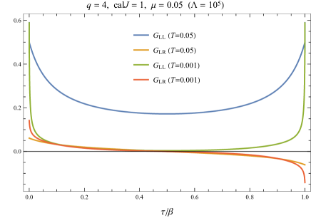
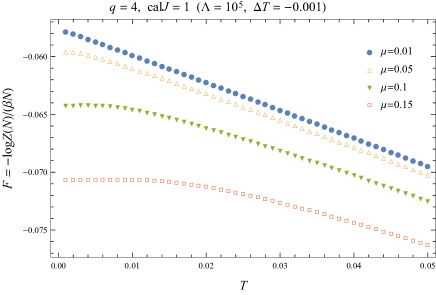
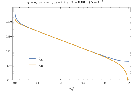
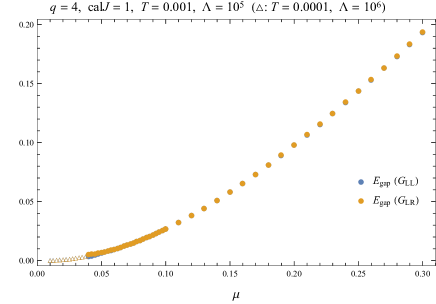
Figure 14: Top left: Euclidean propagator $G_{ab}(\tau)$ of the single sided model with $\mu=0.05$, $T=0.001,0.05$. Top right: Free energy. Bottom left: Euclidean propagator at low temperature $\mu=0.05$, $T=0.001$ where the exponential decay is significant. Bottom right: $E_{\text{gap}}$ of the single sided model obtained by fitting $G_{ab}(\tau)$ at $T=0.001$ ($\mu\geq 0.04$) and at $T=0.0001$ ($\mu\leq 0.03$). For $\mu\leq 0.03$ we have set $\Lambda=10^{6}$.

This model does not exhibit a phase transition regardless of the value of $\mu$ [38]. When the temperature is sufficiently low, however, the Euclidean propagators exhibits exponential decay, which indicates that the system is gapped. We find that $E_{\text{gap}}$ of the single sided model is smaller than that of the two coupled model at same value of $\mu$ and that it behaves as $E_{\text{gap}}\sim\mu^{2}$ at small $\mu$ [38], which is in contrast to the two coupled model where $E_{\text{gap}}\sim\mu^{2/3}$ [23].

The real time propagators also behave similarly to those in the two coupled model both at high temperature and at low temperature. In particular when the temperature is sufficiently low the spectral functions split into sharp peaks, which corresponds to the fact that the system is gapped. The height of the first peak is lower than that for the two coupled model. This is not because the weight $A$ is smaller but rather because the decay width $\Gamma$ is larger. Indeed we have found the decay width of the first peak for the single sided model again obeys the formula (4.7) when the temperature is sufficiently low

$$\Gamma_{\text{1st}}\sim e^{-\frac{1}{2}\beta E_{\text{gap}}}.$$ (4.21)

Here $E_{\text{gap}}$ is the energy gap of the single sided model. See Fig. 16.

Lastly we display the chaos exponent $\lambda_{L}$ in Fig. 17. The overall behavior of the chaos exponent is qualitatively same as that of the two coupled model except the absence of the phase transition. We also observe that $\lambda_{L}$ for the single sided model is always greater than that of the two coupled model at the same values of $(\mu,T)$ as displayed in Fig. 15.

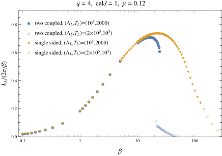
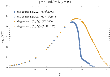
Figure 15: Comparison of the chaos exponent between the two copuled model and the single sided model.

At low temperature we again found that $\lambda_{L}$ obeys (4.8)

$$\lambda_{L}\sim e^{-\frac{1}{2}\beta E_{\text{gap}}}.$$ (4.22)

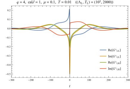
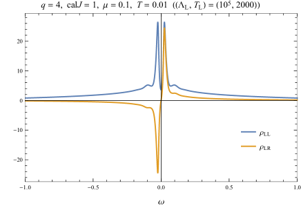
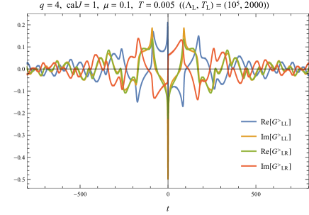
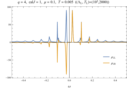
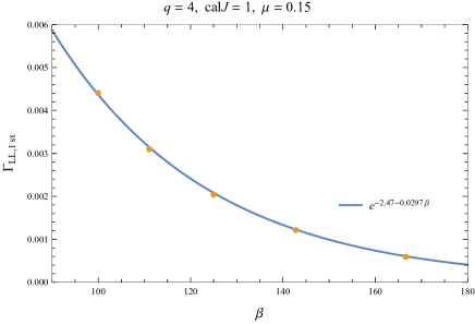
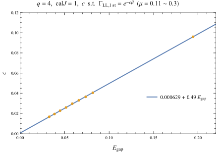
Figure 16: Top left/top right: propagator and spectral function of the single sided model at $\mu=0.1$, $T=0.01$ which are qualitatively same as those in the black hole phase of the two coupled model. Middle left/middle right: propagator and spectral funcntion at $\mu=0.1$, $T=0.01$ where the spectral functions split into well separated peaks as in the wormhole phase of the two coupled model. Bottom left: fitting of the decay width of the first peak with $e^{c_{1}-c_{2}\beta}$, at sufficiently low temperature where the first peak is well separated from the second peak and the mirror of the first peak at $\omega<0$. Bottom right: Comparison of $c_{2}$ with $E_{\text{gap}}$ of the single sided model.

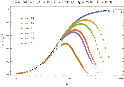
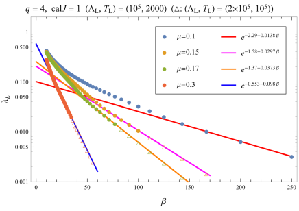
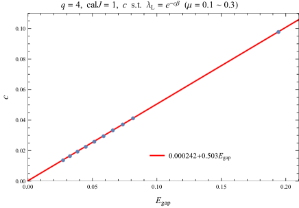
Figure 17: Top left: Chaos exponent $\lambda_{L}$ of the single sided model. Top right: Comparison of $\lambda_{L}$ with the exponential decay $e^{c_{1}-c_{2}\beta}$ obtained by fitting last three to six data points with the largest values of $\beta$ for each $\mu$. Bottom: Comparison of the fitting coefficient $c_{2}$ with $E_{\text{gap}}$.

As $E_{\text{gap}}$ for the single sided model is smaller than that of the two coupled model, this explains the fact that $\lambda_{L}$ for the single sided model is greater than that of the two coupled model. For the same dominance persisting at higher temperature we do not have such clear explanation, but we argue a possible interpretation of it in section 5.

5 Discussion

In this paper we have studied the chaos exponent of the Maldacena-Qi model [23] in detail. The analysis of the level statistics at finite $N$ [31] suggests that there is a quantum chaos transition below $\mu=\mu_{c}=0.177$ where the Hawking-Page like transition in the Maldacena-Qi model disappears. This motivate us to study the chaos exponents, which can be analyzed in the large $N$ limit using the $G,\Sigma$ formalism. Since the Hawking-Page like transition originates from the exchange of the dominance of two different saddles, one may think that the coincidence of the thermal phase transition and a chaos transition is not so surprising. However, it is still non trivial how both phases are characterized from the view of quantum chaos. We have found that when the system goes to the wormhole phase from the black hole phase, the chaos exponent jumps to extremely small values, which is consistent with the expectation in [31].

Another motivation of our analysis is to study the chaos exponent in the gapped phase, which we expect to be an integrable phase. Surprisingly, however, it was found [1] that the two point function shows an exponential decay, which indicates that the system is still chaotic even in this regime. Indeed, we have found that that the chaos exponent is small but non-zero also in the wormhole phase. Moreover, we have found a quantitative relation (4.20) between the chaos exponent and the decay rate which was found to behave as $\Gamma_{\text{1st}}\approx{\cal J}\sqrt{(q-2)!/(2((q/2)!)^{2})}e^{-(q/2-1)E_{\text{gap}}\beta/2}$ [1]. Note that these formulas imply that both the decay rate and the chaos exponent vanishes non-perturbatively in the large $q$ limit with $q\mu$ and $qT$ kept fixed, which is consistent with the fact that we did not observe these chaotic properties in the direct large $q$ analysis [23]. Also note that such a simple relation would not hold in general. For example, in a general conformal field theory the two point function is completely determined by the conformal dimension of the two operators, while to calculate the four point function, which encodes the chaos exponent, we also have to know the OPE coefficients. It would be interesting to understand how the simple relation (4.20) between the chaos exponent and the decay rate, if it exists, will be generalized in other chaotic systems.

We have also found that the slope of the chaos exponent $\partial_{T}\lambda_{L}(T)$ diverges at the end of the two phases $T=T_{c,\text{BH}}$, $T=T_{c,\text{WH}}$. These divergent behaviors resemble that of the energy $E(T)$ and the entropy $S(T)$, rather than of the free energy $F$ whose slope is finite (almost constant) in each phase even near $T_{c,\text{BH}},T_{c,\text{WH}}$. In [23] it was claimed that for $T_{c,\text{BH}}<T<T_{c,\text{WH}}$ there exists another canonically unstable phase throught which the energy varies completely smoothly in the all parameter regime [39]. Although we could not reach the unstable phase in the current analysis, we expect that the chaos exponent shows a similar behavior as the energy, as sketched in Fig. 18. This would be confirmed by solving the Kadanoff-Baym equation of the two coupled system coupled to a cool bath and evaluating the chaos exponent by using the propagators at each time $t_{1}+t_{2}$ before it reaches the equilibrium with $T_{\text{bath}}$ [39, 41, 42].

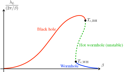
Figure 18: Schematic picture for the expected behavior of the chaos exponent in the unstable hot wormhole phase for $\mu<\mu_{c}$.

We have also considered a model with single SYK with a mass deformation (2.3) [37]. While the single sided model is qualitatively same as the two coupled model in the limit of $\mu\rightarrow 0$ and $\mu\rightarrow\infty$, in contrast to the two coupled model, this model does not exhibit a phase transition. Correspondingly, the chaos exponent we have obtained varies smoothly at all $(\mu,T)$. We have also found that the chaos exponent obeys the same exponential formula $\lambda_{L}\sim e^{-(q/2-1)\beta E_{\text{gap}}/2}$ (1.1) as the decay rate of the first peak [1]. As displayed in appendix A.2, for the single sided model we have reached the low temperature regime also for $q=6,8$, where we have confirmed the formula (1.1) holds also for $q=6,8$.

We have further found that the chaos exponent of the single sided model is always greater than that of the two coupled model in the whole parameter regime. Though in this paper we have regarded the two models in independent ways, we can treat the two models as two different parameter points of a unifed model, where the direct comparison would be more reasonable. We can consider a generalization of the two coupled model with the correlation between the random couplings of the two sides being incomplete $\langle J_{i_{1}i_{2}\cdots i_{q}}^{L}J_{i_{1}i_{2}\cdots i_{q}}^{R}\rangle<\langle(J_{i_{1}i_{2}\cdots i_{q}}^{L})^{2}\rangle=\langle(J_{i_{1}i_{2}\cdots i_{q}}^{R})^{2}\rangle$, where $\langle J_{i_{1}i_{2}\cdots i_{q}}^{L}J_{i_{1}i_{2}\cdots i_{q}}^{R}\rangle/\langle(J_{i_{1}i_{2}\cdots i_{q}}^{L})^{2}\rangle$ is a new tunable parameter of the theory. As we have commented in [38], the single sided model (2.3) is equivanlent to this model with $\langle J^{L}_{i_{1}i_{2}\cdots i_{q}}J^{R}_{i_{1}i_{2}\cdots i_{q}}\rangle/\langle(J^{L}_{i_{1}i_{2}\cdots i_{q}})^{2}\rangle=0$ at the level of the large $N$ $G\Sigma$ formalism. Hence this model unifies the two coupled model and the single sided model, and our observation can be rephrased that the model is less chaotic when $J^{L}_{i_{1}i_{2}\cdots i_{q}}$ and $J^{R}_{i_{1}i_{2}\cdots i_{q}}$ are more correlated. It would be interesting to study the chaotic property of this unifying model and see whether the chaos exponent monotonically decreases with respect to $0<\langle J_{i_{1}i_{2}\cdots i_{q}}^{L}J_{i_{1}i_{2}\cdots i_{q}}^{R}\rangle/\langle(J_{i_{1}i_{2}\cdots i_{q}}^{L})^{2}\rangle<1$ [43].

Appendix A Numerical results for $q=6,8$

A.1 two coupled model

Below we display the results for the phase diagram obtained by solving the Euclidean Schwinger-Dyson equations, and the chaos exponent obtained by solving the real time Schwinger-Dyson equations. See Fig. 19,20. In contrast to the $q=4$ case in the real time analysis we could not reach the convergence in the wormhole regime even with the method of taking $\Lambda/T_{L}$ small explained in the end of section 4.1.2.

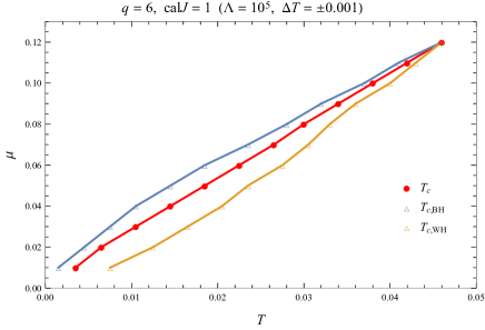
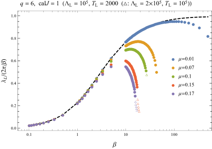
Figure 19: Phase diagram (left) and the chaos exponent (right) of the two coupled model with $q=6$, ${\cal J}=1$.

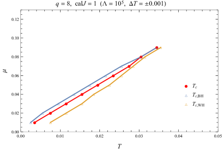
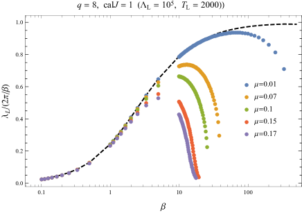
Figure 20: Phase diagram (left) and the chaos exponent (right) of the two coupled model with $q=8$, ${\cal J}=1$.

A.2 single sided model

Below we display the results for the chaos exponent of the single sided model with $q=6,8$. See Fig. 21. As in the case of $q=4$, there are no phase transition. At low temperature we found that the chaos exponent obeys the following formula

$$\lambda_{L}\sim e^{-\frac{q/2-1}{2}\beta E_{\text{gap}}}.$$ (A.1)

Interestingly, this behavior is completely same as that of the decay rate of the first peak [1].

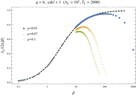
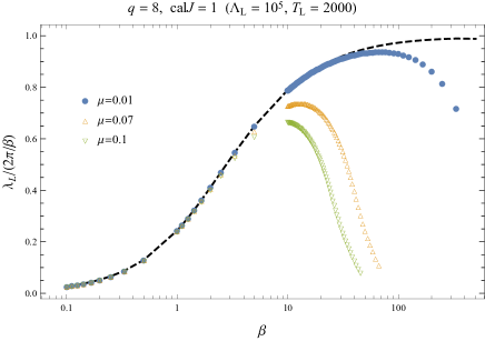
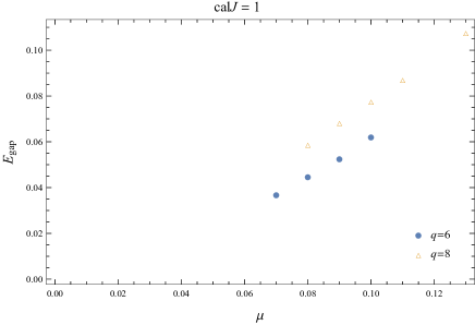
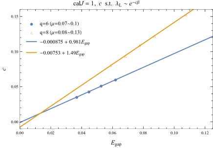
Figure 21: Top left/right: The chaos exponent of the single sided model with $q=6$, ${\cal J}=1$ and $q=8$, ${\cal J}=1$. Bottom left/right: The energy gap $E_{\text{gap}}$ and its comparison with the decay exponent $c$ of the chaos exponent $\lambda_{L}\sim e^{-c\beta}$ at low temperature regime.

References

- [1] X.-L. Qi and P. Zhang, “The Coupled SYK model at Finite Temperature,” JHEP 05 (2020) 129, arXiv:2003.03916 [hep-th].
- [2] S. Sachdev and J. Ye, “Gapless spin-fluid ground state in a random quantum heisenberg magnet,” Phys. Rev. Lett. 70 (May, 1993) 3339–3342. https://link.aps.org/doi/10.1103/PhysRevLett.70.3339.
- [3] A. Kitaev, “A simple model of quantum holography,” talk at KITP strings seminar and Entanglement 2015 program (2015) . http://online.kitp.ucsb.edu/online/entangled15/.
- [4] P. Hayden and J. Preskill, “Black holes as mirrors: Quantum information in random subsystems,” JHEP 09 (2007) 120, arXiv:0708.4025 [hep-th].
- [5] Y. Sekino and L. Susskind, “Fast Scramblers,” JHEP 10 (2008) 065, arXiv:0808.2096 [hep-th].
- [6] A. I. Larkin and Y. N. Ovchinnikov, “Quasiclassical Method in the Theory of Superconductivity,” Soviet Journal of Experimental and Theoretical Physics 28 (Jun, 1969) 1200.
- [7] J. Maldacena and D. Stanford, “Remarks on the Sachdev-Ye-Kitaev model,” Phys. Rev. D94 no. 10, (2016) 106002, arXiv:1604.07818 [hep-th].
- [8] M. V. Berry and M. Tabor, “Level Clustering in the Regular Spectrum,” Proceedings of the Royal Society of London Series A 356 no. 1686, (Sep, 1977) 375–394.
- [9] O. Bohigas, M. J. Giannoni, and C. Schmit, “Characterization of chaotic quantum spectra and universality of level fluctuation laws,” Phys. Rev. Lett. 52 (1984) 1–4.
- [10] J. Maldacena, S. H. Shenker, and D. Stanford, “A bound on chaos,” JHEP 08 (2016) 106, arXiv:1503.01409 [hep-th].
- [11] J. S. Cotler, G. Gur-Ari, M. Hanada, J. Polchinski, P. Saad, S. H. Shenker, D. Stanford, A. Streicher, and M. Tezuka, “Black Holes and Random Matrices,” JHEP 05 (2017) 118, arXiv:1611.04650 [hep-th]. [Erratum: JHEP09,002(2018)].
- [12] H. Gharibyan, M. Hanada, S. H. Shenker, and M. Tezuka, “Onset of Random Matrix Behavior in Scrambling Systems,” JHEP 07 (2018) 124, arXiv:1803.08050 [hep-th]. [Erratum: JHEP 02, 197 (2019)].
- [13] B. Kobrin, Z. Yang, G. D. Kahanamoku-Meyer, C. T. Olund, J. E. Moore, D. Stanford, and N. Y. Yao, “Many-Body Chaos in the Sachdev-Ye-Kitaev Model,” arXiv:2002.05725 [hep-th].
- [14] Y.-Z. You, A. W. W. Ludwig, and C. Xu, “Sachdev-Ye-Kitaev Model and Thermalization on the Boundary of Many-Body Localized Fermionic Symmetry Protected Topological States,” Phys. Rev. B95 no. 11, (2017) 115150, arXiv:1602.06964 [cond-mat.str-el].
- [15] A. M. García-García and J. J. M. Verbaarschot, “Spectral and thermodynamic properties of the Sachdev-Ye-Kitaev model,” Phys. Rev. D94 no. 12, (2016) 126010, arXiv:1610.03816 [hep-th].
- [16] Y. Jia and J. J. Verbaarschot, “Spectral Fluctuations in the Sachdev-Ye-Kitaev Model,” arXiv:1912.11923 [hep-th].
- [17] J. Maldacena, D. Stanford, and Z. Yang, “Conformal symmetry and its breaking in two dimensional Nearly Anti-de-Sitter space,” PTEP 2016 no. 12, (2016) 12C104, arXiv:1606.01857 [hep-th].
- [18] R. Bhattacharya, D. P. Jatkar, and N. Sorokhaibam, “Quantum Quenches and Thermalization in SYK models,” arXiv:1811.06006 [hep-th].
- [19] A. M. García-García and M. Tezuka, “Many-body localization in a finite-range Sachdev-Ye-Kitaev model and holography,” Phys. Rev. B99 no. 5, (2019) 054202, arXiv:1801.03204 [hep-th].
- [20] Y. Gu, X.-L. Qi, and D. Stanford, “Local criticality, diffusion and chaos in generalized Sachdev-Ye-Kitaev models,” JHEP 05 (2017) 125, arXiv:1609.07832 [hep-th].
- [21] A. M. García-García, B. Loureiro, A. Romero-Bermúdez, and M. Tezuka, “Chaotic-Integrable Transition in the Sachdev-Ye-Kitaev Model,” Phys. Rev. Lett. 120 no. 24, (2018) 241603, arXiv:1707.02197 [hep-th].
- [22] T. Nosaka, D. Rosa, and J. Yoon, “The Thouless time for mass-deformed SYK,” JHEP 09 (2018) 041, arXiv:1804.09934 [hep-th].
- [23] J. Maldacena and X.-L. Qi, “Eternal traversable wormhole,” arXiv:1804.00491 [hep-th].
- [24] P. Gao, D. L. Jafferis, and A. C. Wall, “Traversable Wormholes via a Double Trace Deformation,” JHEP 12 (2017) 151, arXiv:1608.05687 [hep-th].
- [25] J. Maldacena, D. Stanford, and Z. Yang, “Diving into traversable wormholes,” Fortsch. Phys. 65 no. 5, (2017) 1700034, arXiv:1704.05333 [hep-th].
- [26] G. Festuccia and H. Liu, “The Arrow of time, black holes, and quantum mixing of large N Yang-Mills theories,” JHEP 12 (2007) 027, arXiv:hep-th/0611098.
- [27] D. A. Roberts, D. Stanford, and L. Susskind, “Localized shocks,” JHEP 03 (2015) 051, arXiv:1409.8180 [hep-th].
- [28] S. H. Shenker and D. Stanford, “Black holes and the butterfly effect,” JHEP 03 (2014) 067, arXiv:1306.0622 [hep-th].
- [29] S. H. Shenker and D. Stanford, “Multiple Shocks,” JHEP 12 (2014) 046, arXiv:1312.3296 [hep-th].
- [30] S. H. Shenker and D. Stanford, “Stringy effects in scrambling,” JHEP 05 (2015) 132, arXiv:1412.6087 [hep-th].
- [31] A. M. García-García, T. Nosaka, D. Rosa, and J. J. M. Verbaarschot, “Quantum chaos transition in a two-site Sachdev-Ye-Kitaev model dual to an eternal traversable wormhole,” Phys. Rev. D100 no. 2, (2019) 026002, arXiv:1901.06031 [hep-th].
- [32] J. M. Maldacena, “Eternal black holes in anti-de Sitter,” JHEP 04 (2003) 021, arXiv:hep-th/0106112.
- [33] I. Amado, B. Sundborg, L. Thorlacius, and N. Wintergerst, “Black holes from large N singlet models,” JHEP 03 (2018) 075, arXiv:1712.06963 [hep-th].
- [34] J. Engelsöy, J. Larana-Aragon, B. Sundborg, and N. Wintergerst, “Operator thermalisation in : Huygens or resurgence,” arXiv:2007.00589 [hep-th].
- [35] S. Plugge, E. Lantagne-Hurtubise, and M. Franz, “Revival dynamics in a traversable wormhole,” Phys. Rev. Lett. 124 no. 22, (2020) 221601, arXiv:2003.03914 [cond-mat.str-el].
- [36] D. Stanford, “Many-body chaos at weak coupling,” JHEP 10 (2016) 009, arXiv:1512.07687 [hep-th].
- [37] I. Kourkoulou and J. Maldacena, “Pure states in the SYK model and nearly- gravity,” arXiv:1707.02325 [hep-th].
- [38] T. Nosaka and T. Numasawa, “Quantum Chaos, Thermodynamics and Black Hole Microstates in the mass deformed SYK model,” arXiv:1912.12302 [hep-th].
- [39] J. Maldacena and A. Milekhin, “SYK wormhole formation in real time,” arXiv:1912.03276 [hep-th].
- [40] E. Lantagne-Hurtubise, S. Plugge, O. Can, and M. Franz, “Diagnosing quantum chaos in many-body systems using entanglement as a resource,” Phys. Rev. Res. 2 no. 1, (2020) 013254, arXiv:1907.01628 [cond-mat.str-el].
- [41] A. Almheiri, A. Milekhin, and B. Swingle, “Universal Constraints on Energy Flow and SYK Thermalization,” arXiv:1912.04912 [hep-th].
- [42] T. Numasawa, Work in Progress.
- [43] T. Nosaka and T. Numasawa, Work in Progress.