Fourier Analysis-based Iterative Combinatorial Auctions

Abstract

Recent advances in Fourier analysis have brought new tools to efficiently represent and learn set functions. In this paper, we bring the power of Fourier analysis to the design of combinatorial auctions (CAs). The key idea is to approximate bidders’ value functions using Fourier-sparse set functions, which can be computed using a relatively small number of queries. Since this number is still too large for practical CAs, we propose a new hybrid design: we first use neural networks (NNs) to learn bidders’ values and then apply Fourier analysis to the learned representations. On a technical level, we formulate a Fourier transform-based winner determination problem and derive its mixed integer program formulation. Based on this, we devise an iterative CA that asks Fourier-based queries. We experimentally show that our hybrid ICA achieves higher efficiency than prior auction designs, leads to a fairer distribution of social welfare, and significantly reduces runtime. With this paper, we are the first to leverage Fourier analysis in CA design and lay the foundation for future work in this area. Our code is available on GitHub: https://github.com/marketdesignresearch/FA-based-ICAs.

1 Introduction

Combinatorial auctions (CAs) are used to allocate multiple heterogeneous items to bidders. CAs are particularly useful in domains where bidders’ preferences exhibit complementarities and substitutabilities as they allow bidders to submit bids on bundles of items rather than on individual items.

Since the bundle space grows exponentially in the number of items, it is impossible for bidders to report values for all bundles in settings with more than a modest number of items. Thus, parsimonious preference elicitation is key for the practical design of CAs. For general value functions, Nisan and Segal Nisan and Segal (2006) have shown that to guarantee full efficiency, exponential communication in the number of items is needed. Thus, practical CAs cannot provide efficiency guarantees in large domains. Instead, recent proposals have focused on iterative combinatorial auctions (ICAs), where the auctioneer interacts with bidders over rounds, eliciting a limited amount of information, aiming to find a highly efficient allocation.

ICAs have found widespread application; most recently, for the sale of licenses to build offshore wind farms Ausubel and Cramton (2011). For the sale of spectrum licenses, the combinatorial clock auction (CCA) Ausubel et al. (2006) has generated more than $20 billion in total revenue Ausubel and Baranov (2017). Thus, increasing the efficiency by only 1–2% points translates into monetary gains of millions of dollars.

1.1 Machine Learning-based Auction Design

Recently, researchers have used machine learning (ML) to improve the performance of CAs. Early work by Blum et al. Blum et al. (2004) and Lahaie and Parkes Lahaie and Parkes (2004) first studied the relationship between learning theory and preference elicitation in CAs. Dütting et al. Dütting et al. (2019), Shen et al. Shen et al. (2019) and Rahme et al. Rahme et al. (2021) used neural networks (NNs) to learn whole auction mechanisms from data. Brero et al. Brero et al. (2019) introduced a Bayesian ICA using probabilistic price updates to achieve faster convergence. Shen et al. Shen et al. (2020) use reinforcement learning for dynamic pricing in sponsored search auctions. Most related to the present paper is the work by Brero et al. Brero et al. (2018, 2021), who developed a value-query-based ML-powered ICA using support vector regressions (SVRs) that achieves even higher efficiency than the CCA. In follow-up work, Weissteiner and Seuken Weissteiner and Seuken (2020) extended their ICA to NNs, further increasing the efficiency. In work subsequent to the first version of this paper, Weissteiner et al. Weissteiner et al. (2022a) proposed Monotone-Value Neural Networks (MVNNs), which are particularly well suited to learning value functions in combinatorial assignment domains.

However, especially in large domains, it remains a challenge to find the efficient allocation while keeping the elicitation cost low. Thus, even state-of-the-art approaches suffer from significant efficiency losses and often result in unfair allocations, highlighting the need for better preference elicitation algorithms.

1.2 Combining Fourier Analysis and CAs

The goal of preference elicitation in CAs is to learn bidders’ value functions using a small number of queries. Mathematically, value functions are set functions, which are in general exponentially large and notoriously hard to represent or learn. To address this complexity, we leverage Fourier analysis for set functions Bernasconi et al. (1996); O’Donnell (2014); Püschel and Wendler (2020). In particular, we consider Fourier-sparse approximations, which are represented by few parameters. These parameters are the non-zero Fourier coefficients (FCs) obtained by a base change with the Fourier transform (FT). We use the framework by Püschel and Wendler Püschel and Wendler (2020), which contains new FTs beyond the classical Walsh-Hadamard transform (WHT) Bernasconi et al. (1996), providing more flexibility. Until recently, methods for learning Fourier-sparse set functions focused on the WHT, and they placed assumptions on bidders’ value functions that are too restrictive for CAs Stobbe and Krause (2012). However, recently, Amrollahi et al. Amrollahi et al. (2019) proposed a new algorithm that can approximate general set functions by WHT-sparse ones, which is suitable for large CAs and we use it in this work.

1.3 Our Contribution

Our main contribution in this paper is to bring the power of Fourier analysis to CA design (Section 3). In particular, we formulate FT-based winner determination problems (WDPs) and derive corresponding mixed integer programs (MIPs) for several FTs (Section 4). Our MIPs allow for the efficient solution of the FT-based WDP and provide the foundation for using Fourier-sparse approximations in auction design.

We first experimentally show that the WHT performs best among the FTs in terms of induced level of sparsity (Section 5.1) and reconstruction error (Section 5.2). As an initial approach, we develop a WHT-based allocation rule (Section 5.3). However, this requires too many queries for direct use in CAs. To overcome this, we propose a practical hybrid ICA based on NNs and Fourier analysis (Section 6.1). The key idea is to compute Fourier-sparse approximations of NN-based bidder representations, enabling us to keep the number of queries small. The advantage of the NN-based representations is that they capture key aspects of the bidders’ value functions and can be queried arbitrarily often (Section 6.2).

Our efficiency experiments show that our hybrid ICA achieves higher efficiency than state-of-the-art mechanisms, leads to a significant computational speedup, and yields fairer allocations (Section 6.3). This shows that leveraging Fourier analysis in CA design is a promising new research direction.

2 Preliminaries

In this section, we present our formal model and review the MLCA mechanism, which our hybrid ICA builds upon.

2.1 Formal Model for ICAs

We consider a CA with $n$ bidders and $m$ indivisible items. Let $N=\{1,\ldots,n\}$ and $M=\{1,\ldots,m\}$ denote the set of bidders and items, respectively. We denote with $x\in\mathcal{X}=\{0,1\}^{m}$ a bundle of items represented as an indicator vector, where $x_{j}=1$ iff item $j\in M$ is contained in $x$. Bidders’ true preferences over bundles are represented by their (private) value functions $v_{i}:\mathcal{X}\to\mathbb{R}_{+},\,\,i\in N$, i.e., $v_{i}(x)$ represents bidder $i$’s true value for bundle $x$. By $a=(a_{1},\ldots,a_{n})\in\mathcal{X}^{n}$ we denote an allocation of bundles to bidders, where $a_{i}$ is the bundle bidder $i$ obtains. We denote the set of feasible allocations by $\mathcal{F}=\left\{a\in\mathcal{X}^{n}:\sum_{i\in N}a_{ij}\leq 1,\,\,\forall j\in M\right\}$. The (true) social welfare of an allocation $a$ is defined as $V(a)=\sum_{i\in N}v_{i}(a_{i}).$ We let $a^{*}\in\operatorname*{argmax}_{a\in{\mathcal{F}}}V(a)$ be a social-welfare maximizing, i.e., efficient, allocation. The efficiency of any $a\in\mathcal{F}$ is measured by $V(a)/V(a^{*})$. We assume that bidders’ have quasilinear utilities $u_{i}$, i.e, for a payments $p\in\mathbb{R}^{n}_{+}$ it holds that $u_{i}(a,p)=v_{i}(a_{i})-p_{i}$.

An ICA mechanism defines how the bidders interact with the auctioneer and how the final allocation and payments are determined. We denote a bidder’s (possibly untruthful) reported value function by $\hat{v}_{i}:\mathcal{X}\to\mathbb{R}_{+}$. In this paper, we consider ICAs that ask bidders iteratively to report their value $\hat{v}_{i}(x)$ for particular bundles $x$ selected by the mechanism (for early work on value queries see Hudson and Sandholm (2003)). A finite set of such reported bundle-value pairs of bidder $i$ is denoted as ${R_{i}=\left\{\left(x^{(l)},\hat{v}_{i}(x^{(l)})\right)\right\},\,x^{(l)}\in\mathcal{X}}$. Let $R=(R_{1},\ldots,R_{n})$ denote the tuple of reported bundle-value pairs obtained from all bidders. We define the reported social welfare of an allocation $a$ given $R$ as $\widehat{V}(a|R)=\sum_{i\in N:\,\left(a_{i},\hat{v}_{i}(a_{i})\right)\in R_{i}}\hat{v}_{i}(a_{i}),$ where $\left(a_{i},\hat{v}_{i}(a_{i})\right)\in R_{i}$ ensures that only values for reported bundles contribute. Finally, the optimal allocation $a^{*}_{R}\in\mathcal{F}$ given the reports $R$ is defined as

$$a^{*}_{R}\in\operatorname*{argmax}_{a\in{\mathcal{F}}}\widehat{V}(a|R).$$ (1)

The final allocation $a^{*}_{R}\in\mathcal{F}$ and payments $p(R)\in\mathbb{R}^{n}_{+}$ are computed based on the elicited reports $R$ only.

As the auctioneer can only ask each bidder $i$ a limited number of queries $|R_{i}|\leq Q^{\textrm{\tiny max}}$, the ICA needs a smart preference elicitation algorithm, with the goal of finding a highly efficient $a^{*}_{R}$ with a limited number of value queries.

2.2 A Machine Learning-powered ICA

We now review the machine learning-powered combinatorial auction (MLCA) by Brero et al. Brero et al. (2021). Interested readers are referred to Section A.1, where we present MLCA in detail.

MLCA starts by asking each bidder value queries for $Q^{\textrm{\tiny init}}$ randomly sampled initial bundles. Next, MLCA proceeds in rounds until a maximum number of value queries per bidder $Q^{\textrm{\tiny max}}$ is reached. In each round, for each bidder $i\in N$, it trains an ML algorithm $\mathcal{A}_{i}$ on the bidder’s reports $R_{i}$. Next, MLCA generates new value queries $q^{\textrm{\tiny new}}=(q^{\textrm{\tiny new}}_{i})_{i=1}^{n}$ with $q^{\textrm{\tiny new}}_{i}\in\mathcal{X}\setminus R_{i}$ by solving a ML-based WDP $q^{\textrm{\tiny new}}\in\operatorname*{argmax}\limits_{a\in{\mathcal{F}}}\sum\limits_{i\in N}\mathcal{A}_{i}(a_{i})$. The idea is the following: if $\mathcal{A}_{i}$ are good surrogate models of the bidders’ true value functions then $q^{\textrm{\tiny new}}$ should be a good proxy of the efficient allocation $a^{*}$ and thus provide valuable information.

At the end of each round, MLCA receives reports $R^{\textrm{\tiny new}}$ from all bidders for the newly generated $q^{\textrm{\tiny new}}$ and updates $R$. When $Q^{\textrm{\tiny max}}$ is reached, MLCA computes an allocation $a^{*}_{R}$ maximizing the reported social welfare (eq. 1) and determines VCG payments $p(R)$ (see Section A.2).

2.3 Incentives of MLCA and Hybrid ICA

A key concern in the design of ICAs are bidders’ incentives. However, the seminal result by Nisan and Segal Nisan and Segal (2006) discussed above implies that practical ICAs cannot simply use VCG to achieve strategyproofness. And in fact, no ICA deployed in practice is strategyproof – including the famous SMRA and CCA auctions used to conduct spectrum auctions. Instead, auction designers have designed mechanisms that, while being manipulable, have “good incentives in practice” (see Cramton (2013); Milgrom (2007)).

Naturally, the MLCA mechanism is also not strategyproof, and Brero et al. Brero et al. (2021) provide a simple example of a possible manipulation. The idea behind the example is straightforward: if the ML algorithm does not learn a bidder’s preferences perfectly, a sub-optimal allocation may result. Thus, a bidder may (in theory) benefit from misreporting their preferences with the goal of “correcting” the ML algorithm, so that, with the misreported preferences, the mechanism actually finds a preferable allocation.

However, MLCA has two features that mitigate manipulations. First, MLCA explicitly queries each bidder’s marginal economy, which implies that the marginal economy term of the final VCG payment is practically independent of bidder $i$’s bid (for experimental support see Brero et al. (2021)). Second, MLCA enables bidders to “push” information to the auction which they deem useful. This mitigates certain manipulations of the main economy term in the VCG payment rule, as it allows bidders to increase the social welfare directly by pushing (useful) truthful information, rather than attempting to manipulate the ML algorithm. Brero et al. Brero et al. (2021) argued that with these two design features, MLCA exhibits very good incentives in practice. They performed a computational experiment, testing whether an individual bidder (equipped with more information than he would have in a real auction) can benefit from deviating from truthful bidding, while all other bidders are truthful. In their experiments, they could not identify a beneficial manipulation strategy. While this does not rule out that some (potentially more sophisticated) beneficial manipulations do exist, it provides evidence to support the claim that MLCA has good incentives in practice.

With two additional assumptions, one also obtains a theoretical incentive guarantee for MLCA. Assumption 1 requires that, if all bidders bid truthfully, then MLCA finds an efficient allocation (we show in Section D.3 that in two of our domains, we indeed find the efficient allocation in the majority of cases). Assumption 2 requires that, for all bidders $i$, if all other bidders report truthfully, then the social welfare of bidder $i$’s marginal economy is independent of his value reports. If both assumptions hold, then bidding truthfully is an ex-post Nash equilibrium in MLCA.

Our hybrid ICA (Algorithm 1 in Section 6.1) is built upon MLCA, leaving the general framework in place, and only changing the algorithm that generates new queries each round. Given this design, the incentive properties of MLCA extend to the hybrid ICA. Specifically, our hybrid ICA is also not strategyproof, but it also has the same design features (including push-bids) to mitigate manipulations.

In future work, it would be interesting to evaluate experimentally whether the improved performance of the hybrid ICA translates into better manipulation mitigation compared to MLCA. However, such an analysis is beyond the scope of the present paper, which focuses on the ML algorithm that is integrated into the auction mechanism.

3 Fourier Analysis of Value Functions

We now show how to apply Fourier analysis to value functions providing the theoretical foundation of FT-based WDPs.

Classic Fourier analysis decomposes an audio signal or image into an orthogonal set of sinusoids of different frequencies. Similarly, the classical Fourier analysis for set functions (i.e., functions mapping subsets of a discrete set to a scalar) decomposes a set function into an orthogonal set of Walsh functions Bernasconi et al. (1996), which are piecewise constant with values $1$ and $-1$ only. Recent work by Püschel and Wendler Püschel and Wendler (2020) extends the Fourier analysis for set functions with several novel forms of set Fourier transforms (FTs). Importantly, because bidders’ value functions are set functions, they are amenable to this type of Fourier analysis, and it is this connection that we will leverage in our auction design.

Sparsity. The motivation behind our approach is that we expect bidders’ value functions to be sparse, i.e., they can be described with much less data than is contained in the exponentially-sized full value function. While this sparsity may be difficult to uncover when looking at bidders’ value reports directly, it may reveal itself in the Fourier domain (where then most FCs are zero). As all FTs are changes of basis, each FT provides us with a new lens on the bidder’s value function, revealing structure and thus potentially reducing dimensionality.

Set function Fourier transform. We now provide a formal description of FTs for reported value functions $\hat{v}_{i}$. To do so, we represent $\hat{v}_{i}$ as a vector $(\hat{v}_{i}(x))_{x\in\mathcal{X}}$. Each known FT is a change of basis and thus can be represented by a certain matrix $F\in\{-1,0,1\}^{2^{m}\times 2^{m}}$ with the form:

$$\phi_{\hat{v}_{i}}(y)=(F\hat{v}_{i})({y})=\sum_{x\in\mathcal{X}}F_{y,x}\hat{v}_{i}(x).$$ (2)

There is exactly one Fourier coefficient per bundle, this follows from the theory presented by Püschel and Wendler Püschel and Wendler (2020). The corresponding inverse transform $F^{-1}$ is thus:

$$\hat{v}_{i}(x)=(F^{-1}\phi_{\hat{v}_{i}})(x)=\sum_{y\in\mathcal{X}}F^{-1}_{x,y}\phi_{\hat{v}_{i}}(y).$$ (3)

$\phi_{\hat{v}_{i}}$ is again a set function and we call $\phi_{\hat{v}_{i}}(y)$ the Fourier coefficient at frequency $y$. A value function is Fourier-sparse if $|\operatorname*{supp}(\phi_{\hat{v}_{i}})|=|\{y:\phi_{\hat{v}_{i}}(y)\neq 0\}|\ll 2^{m}$. We call $\operatorname*{supp}(\phi_{\hat{v}_{i}})$ the Fourier support of $\hat{v}_{i}$.

Classically, the WHT is used as $F$ Bernasconi et al. (1996); O’Donnell (2014), but we also consider two recently introduced FTs (FT3, FT4) due to their information-theoretic interpretation given in Püschel and Wendler (2020):

FT3: $$F_{y,x}=(-1)^{|y|-|x|}\mathbb{I}_{\min(x,y)=x},$$ (4)

FT4: $$F_{y,x}=(-1)^{|\min(x,y)|}\mathbb{I}_{\max(x,y)=1_{m}},$$ (5)

WHT: $$F_{y,x}=\frac{1}{2^{m}}(-1)^{|\min(x,y)|}.$$ (6)

Here, $\min$ is the elementwise minimum (intersection of sets), $\max$ analogously, $|\cdot|$ is the set size, $1_{m}$ denotes the $m$-dimensional vector of 1s, and the indicator function $\mathbb{I}_{P}$ is equal to $1$ if the predicate $P$ is true and $0$ otherwise.

Notions of Fourier-sparsity. In recent years, the notion of Fourier-sparsity has gained considerable attention, leading to highly efficient algorithms to compute FTs Stobbe and Krause (2012); Amrollahi et al. (2019); Wendler et al. (2021). Many classes of set functions are Fourier-sparse (e.g., graph cuts, hypergraph valuations and decision trees Abraham et al. (2012)) and can thus be learned efficiently. The benefit of considering multiple FTs is that they offer different, non-equivalent notions of sparsity as illustrated by the following example.

Example 1.

Consider the set of items $M=\{1,2,3\}$ and the associated reported value function $\hat{v}_{i}$ shown in Table 1 (where we use $001$ as a shorthand notation for $(0,0,1)$), together with the corresponding FCs $\phi_{\hat{v}_{i}}$:

	000	100	010	001	110	101	011	111
$\hat{v}_{i}$	0	1	1	1	3	3	3	5
FT3	0	1	1	1	1	1	1	-1
FT4	5	-2	-2	-2	0	0	0	1
WHT	$\nicefrac{{17}}{{8}}$	-$\nicefrac{{7}}{{8}}$	-$\nicefrac{{7}}{{8}}$	-$\nicefrac{{7}}{{8}}$	$\nicefrac{{1}}{{8}}$	$\nicefrac{{1}}{{8}}$	$\nicefrac{{1}}{{8}}$	$\nicefrac{{1}}{{8}}$

Table 1: Example with different induced notions of sparsity of all considered FTs.

This bidder exhibits complementary effects for each bundle containing more than one item, as can be seen, e.g., from $3=\hat{v}_{i}(110)>\hat{v}_{i}(100)+\hat{v}_{i}(010)=2$ and $5=\hat{v}_{i}(111)>\hat{v}_{i}(100)+\hat{v}_{i}(010)+\hat{v}_{i}(001)=3$. Observe that while this value function is sparse in FT4, i.e., $\phi_{\hat{v}_{i}}(110)=\phi_{\hat{v}_{i}}(101)=\phi_{\hat{v}_{i}}(011)=0$, it is neither sparse in FT3 nor WHT. Note that the coefficients $\phi_{\hat{v}_{i}}(100)$, $\phi_{\hat{v}_{i}}(010)$, and $\phi_{\hat{v}_{i}}(001)$ capture the value of single items and thus cannot be zero.

The induced spectral energy distributions for each FT, i.e., for each cardinality (i.e., number of items) $d$ from $0$ to $m=3$, we compute $\sum_{y\in\mathcal{X}:|y|=d}\phi_{\hat{v}_{i}}(y)^{2}/\sum_{y\in\mathcal{X}}\phi_{\hat{v}_{i}}(y)^{2}$, are shown in Table 2.

	$d=0$	$d=1$	$d=2$	$d=3$
FT3	$00.00$	$42.86$	$42.86$	$14.28$
FT4	$65.79$	$31.58$	$00.00$	$02.63$
WHT	$65.69$	$33.41$	$00.68$	$00.22$

Table 2: Spectral energy in $\%$ for each cardinality (i.e., number of items) $d$ from $0$ to $m=3$ of all considered FTs.

Fourier-sparse approximations. In practice, $\hat{v}_{i}$ may only be approximately sparse. Meaning that while not being sparse, it can be approximated well by a Fourier-sparse function $\tilde{v}_{i}$. Formally, let $\mathcal{S}_{i}=\operatorname*{supp}(\phi_{\tilde{v}_{i}})$ with $|\mathcal{S}_{i}|=k$, we call

$$\tilde{v}_{i}(x)=\sum_{y\in\mathcal{S}_{i}}F^{-1}_{x,y}\phi_{\tilde{v}_{i}}(y)\text{ for all }x\in\mathcal{X}$$ (7)

such that $\|\tilde{v}_{i}-\hat{v}_{i}\|_{2}$ is small a $k$-Fourier-sparse approximation of $\hat{v}_{i}$. We denote the vector of FCs by ${\phi_{\tilde{v}_{i}|\mathcal{S}_{i}}=(\phi_{\tilde{v}_{i}}(y))_{y\in\mathcal{S}_{i}}}$.

4 Fourier Transform-based WDPs

To leverage Fourier analysis for CA design, we represent bidders’ value functions using Fourier-sparse approximations. A key step in most auction designs is to find the social welfare-maximizing allocation given bidder’s reports, which is known as the Winner Determination Problem (WDP). To apply FTs, we need to be able to solve the WDP efficiently. Accordingly, we next derive MIPs for each of the FTs.

For each bidder $i\in N$, let $\tilde{v}_{i}:\mathcal{X}\to\mathbb{R}_{+}$ be a Fourier-sparse approximation of the bidders’ reported value function $\hat{v}_{i}$. Next, we define the Fourier transform-based WDP.

Definition 1.

(Fourier transform-based WDP)

$$\operatorname*{argmax}\limits_{a\in\mathcal{F}}\sum_{i\in N}\tilde{v}_{i}(a_{i}).$$ (FT-WDP)

For $x,y\in\mathbb{R}^{d},$ let $x\leq y,\,\max(x,y)$ and $\left(-1\right)^{x}$ be defined component-wise, and let $\langle\cdot,\cdot\rangle$ denote the Euclidean scalar product. First, we formulate succinct representations of $\tilde{v}_{i}$.

Lemma 1.

For $i\in N$ let $\mathcal{S}_{i}=\{y^{(1)},\dots,y^{(k)}\}$ be the support of a $k$-Fourier-sparse approximation $\tilde{v}_{i}$ and $W_{i}\in\{0,1\}^{k\times m}$ be defined as $\left(W_{i}\right)_{l,j}=\mathbb{I}_{y^{(l)}_{j}=1}$. Then it holds that

FT3: $$\tilde{v}_{i}(x)=\left\langle\phi_{\tilde{v}_{i}|\mathcal{S}_{i}},\max\left(0_{k},1_{k}-W_{i}(1_{m}-x)\right)\right\rangle$$ (8)

FT4: $$\tilde{v}_{i}(x)=\left\langle\phi_{\tilde{v}_{i}|\mathcal{S}_{i}},\max\left(0_{k},1_{k}-W_{i}x\right)\right\rangle$$ (9)

WHT: $$\tilde{v}_{i}(x)=\left\langle\phi_{\tilde{v}_{i}|\mathcal{S}_{i}},(-1)^{W_{i}x}\right\rangle.$$ (10)

See Section B.1 for the proof. With Lemma 1 and rewriting $\max(\cdot,\cdot)$ and $(-1)^{\cdot}$ as linear constraints, we next encode (FT-WDP) as a MIP (see Section B.2 for the proof).

Theorem 1.

(FT-based MIPs) Let $\tilde{v}_{i}:\mathcal{X}\to\mathbb{R}$ be a k-Fourier-sparse approximation from (8), (9), or (10). Then there exists a $C>0$ s.t. the MIP defined by the objective

$$\operatorname*{argmax}\limits_{a\in\mathcal{F},\beta_{i}\in\{0,1\}^{k}}\sum_{i\in N}\langle\phi_{\tilde{v}_{i}|\mathcal{S}_{i}},\alpha_{i}\rangle,$$ (11)

and for $i\in N$ one set of transform specific constraints (12)–(14), or (15)–(17), or (18)–(20), is equivalent to (FT-WDP).

FT3:s.t. $$\alpha_{i}\geq 1_{k}-W_{i}(1_{m}-a_{i})$$ (12)

$$\alpha_{i}\leq 1_{k}-W_{i}(1_{m}-a_{i})+C\beta_{i}$$ (13)

$$0_{k}\leq\alpha_{i}\leq C(1_{k}-\beta_{i})$$ (14)

FT4:s.t. $$\alpha_{i}\geq 1_{k}-W_{i}a_{i}$$ (15)

$$\alpha_{i}\leq 1_{k}-W_{i}a_{i}+C\beta_{i}$$ (16)

$$0_{k}\leq\alpha_{i}\leq C(1_{k}-\beta_{i})$$ (17)

WHT:s.t. $$\alpha_{i}=-2\beta_{i}+1_{k}$$ (18)

$$\beta_{i}=W_{i}a_{i}-2\gamma_{i}$$ (19)

$$\gamma_{i}\in\mathbb{Z}^{k}$$ (20)

5 Analyzing the Potential of a FT-based CA

In this section, we experimentally evaluate the FTs and propose an FT-based allocation rule that motivates our practical hybrid ICA mechanism presented later in Section 6.

For our experiments, we use the spectrum auction test suite (SATS) Weiss et al. (2017). SATS enables us to generate synthetic CA instances in different domains. We have access to each bidder’s true full value function $v_{i}$ and the efficient allocation $a^{*}$. When simulating bidders, we assume truthful bidding (i.e., $\hat{v}_{i}=v_{i}$). We consider three domains:

The Global Synergy Value Model (GSVM) Goeree and Holt (2010) has $18$ items, $6$ regional and $1$ national bidder.

The Local Synergy Value Model (LSVM) Scheffel et al. (2012) consists of $18$ items, $5$ regional and $1$ national bidder. Complementarities arise from spatial proximity of items.

The Multi-Region Value Model (MRVM) Weiss et al. (2017) has $98$ items and $10$ bidders (categorized as local, regional, or national) and models large US spectrum auctions.

5.1 Notions of Fourier Sparsity

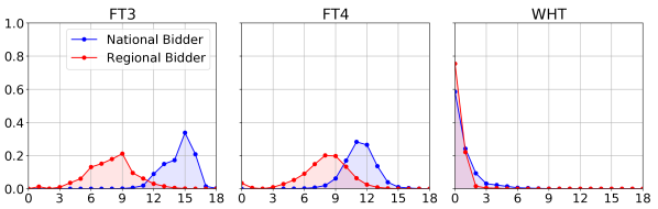
Figure 1: Spectral energy distribution in LSVM for all FTs. For each cardinality (x-axis), we plot the spectral energy of all frequencies of that cardinality normalized by the total spectral energy (y-axis).

We first experimentally show that different notions of FT lead to different types of sparsity in LSVM (for other domains see Section C.1). For this we first compute the FTs of all bidders and then calculate their spectral energy distribution. That is, for each cardinality $d$ (#items) from $0$ to $m$, we compute $\sum_{y\in\mathcal{X}:|y|=d}\phi_{\hat{v}_{i}}(y)^{2}/\sum_{y\in\mathcal{X}}\phi_{\hat{v}_{i}}(y)^{2}$. In Figure 1, we present the mean over 30 LSVM instances and bidder types.

Figure 1 shows that while the energy is spread among FCs of various degrees in FT3 and FT4, in WHT the low degree ($\leq 2$) FCs contain most of the energy, i.e., the WHT has much fewer dominant FCs that accurately describe each value function. As the WHT is orthogonal, learning low degree WHT-sparse approximations leads to low reconstruction error. Low degree WHT-sparse approximations can be learnt efficiently and accurately from a small number of queries using compressive sensing Stobbe and Krause (2012).

Note that the FT3 is identical to the classical polynomial value function representation Lahaie (2010) defined as

$$\hat{v}_{i}^{\text{poly}}(x)=\sum_{l=1}^{m}\sum_{\boldsymbol{j}=\{j_{1},\ldots,j_{l}\}\subseteq M}x_{j_{1}}\cdot...\cdot x_{j_{l}}\cdot c^{(i)}_{\boldsymbol{j}}.$$ (21)

where the coefficient $c^{(i)}_{\boldsymbol{j}}$ is equal to the FT3 FC at frequency $y$ with $y_{i}=1$ for $i\in\{j_{1},\dots,j_{l}\}$ and $y_{i}=0$ else. E.g. for $M=\{1,2\},$ $\hat{v}_{i}^{\text{poly}}(x)=x_{1}c^{(i)}_{\{1\}}+x_{2}c^{(i)}_{\{2\}}+x_{1}x_{2}c^{(i)}_{\{1,2\}}$. Thus, converting $\hat{v}_{i}^{\text{poly}}$ into another FT basis (here WHT) can indeed be very helpful for the design of ML-based CAs.

5.2 Reconstruction Error of Fourier Transforms

Next we validate the FT approach by comparing the reconstruction error of the FTs in the medium-sized GSVM and LSVM, where we can still compute the full FT (in contrast to MRVM). For now, we assume that we have access to bidders’ full $\hat{v}_{i}$. In Procedure 5.2, we determine the best $k$-Fourier-sparse approximation $\tilde{v}_{i}$ (see Section C.2 for details).

(Best FCs Given Full Access to $\hat{v}_{i}$) 
Compute $\tilde{v}_{i}$ using the $k$ absolutely largest FCs $\phi_{\hat{v}_{i}|\mathcal{S}_{i}}$ from the full FT for each bidders’ reported value function $\phi_{\hat{v}_{i}}=F\hat{v}_{i}$.

Remark 1.

Since the WHT is orthogonal and the simulated auction data is noise-free, its approximation error is exactly equal to the residual of the FCs. Thus, Procedure 5.2 is optimal for the WHT. This is not the case for FT3 and FT4 because they are not orthogonal.

Domain	k	Bidder	FT3	FT4	WHT	NN
GSVM	100	Nat.	$11.3\pm 0.7$	$14.2\pm 0.8$	$1.8\pm 0.1$	$9.0\pm 1.8$
		Reg.	$0.0\pm 0.0$	$1.4\pm 0.2$	$0.4\pm 0.1$	$7.2\pm 0.9$
	200	Nat.	$0.0\pm 0.0$	$0.0\pm 0.0$	$0.0\pm 0.0$	$5.7\pm 0.4$
		Reg.	$0.0\pm 0.0$	$0.0\pm 0.0$	$0.0\pm 0.0$	$5.2\pm 0.8$
LSVM	100	Nat.	$78.4\pm 1.0$	$580.2\pm 7.9$	$31.2\pm 0.4$	$48.7\pm 1.2$
		Reg.	$28.2\pm 2.3$	$48.5\pm 2.7$	$6.8\pm 0.3$	$17.8\pm 0.7$
	200	Nat.	$95.8\pm 1.2$	$639.0\pm 10.0$	$26.2\pm 0.3$	$40.6\pm 0.7$
		Reg.	$25.8\pm 2.0$	$43.1\pm 2.4$	$5.3\pm 0.3$	$15.3\pm 0.9$

Table 3: Reconstruction error with a $95\%$-CI of $k$-Fourier-sparse approximations $\tilde{v}_{i}$ and NNs trained on $k$ randomly selected bundles. Winners are marked in grey.

We then calculate the RMSE ${\scriptsize(\frac{1}{2^{m}}\sum_{x\in\mathcal{X}}(\hat{v}_{i}(x)-\tilde{v}_{i}(x))^{2})^{\nicefrac{{1}}{{2}}}}$ averaged over 100 instances and bidder types. In Table 3, we present the RMSEs for the three FTs and for NNs, where we used the architectures from Weissteiner and Seuken Weissteiner and Seuken (2020).

For GSVM, we observe that we can perfectly reconstruct $\hat{v}_{i}$ with the $200$ best FCs, which shows that GSVM is 200-sparse. In contrast, LSVM is non-sparse, and we do not achieve perfect reconstruction with $200$ FCs. Overall, we observe that the WHT outperforms FT3 and FT4. Moreover, we see that, if we could compute the $k$ best FCs of the WHT from $k$ training points, the WHT would outperform the NNs.

However, in practice, we do not have access to full value functions. Instead, we must use an algorithm that computes the best FCs using a reasonable number of value queries.

Remark 2.

Thanks to its orthogonality the WHT has strong theoretical guarantees for sparse recovery from few samples using compressive sensing (see Stobbe and Krause (2012)). Thus, we focus on the WHT in the remainder of this paper.

5.3 A Fourier Transform-based Allocation Rule

We now present an FT-based allocation rule using the robust sparse WHT algorithm (RWHT) by Amrollahi et al. Amrollahi et al. (2019). RWHT learns a Fourier-sparse approximation $\tilde{v}_{i}$ of $\hat{v}_{i}$ from value queries. Procedure 5.3 finds the allocation $\tilde{a}$. (WHT-based Allocation Rule)

i. Use RWHT to compute $k$-sparse approximations $\tilde{v}_{i}\,,i\in N$.

ii. Solve ${\tilde{a}\in\operatorname*{argmax}\limits_{a\in\mathcal{F}}\sum\limits_{i\in N}\tilde{v}_{i}(a_{i})}$ using Theorem 1.

In Figure 2, we present the efficiency of $\tilde{a}$ on 50 GSVM instances for various values of $k$. We see that RWHT achieves a median efficiency of 100% for $90$ or more FCs. Nevertheless, the main practical issue with this approach is the number of value queries required. As we can see, RWHT needs $102,000$ value queries (39% of all bundles) to find the $90$ best FCs. For a practical ICA mechanism this is far too many.

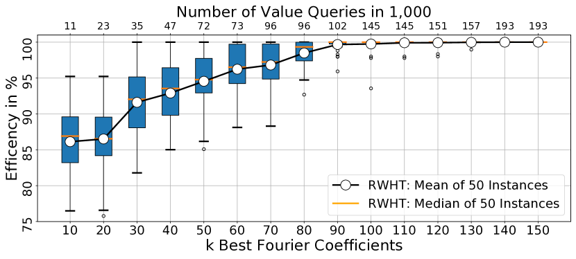
Figure 2: Efficiency of Procedure 2 in GSVM.

6 A Practical Hybrid ICA Mechanism

In this section, we introduce and experimentally evaluate a practical hybrid ICA mechanism, based on FTs and NNs.

6.1 The Hybrid ICA Mechanism

The main issue of the FT-based allocation rule in Section 5.3 is the large number of queries, which we now address. The idea is the following: instead of directly applying a sparse FT algorithm (like RWHT) to bidders, we apply it to a NN-based representation. In this way, we query NNs instead of bidders. Based on the FCs of the NNs, we determine a Fourier-sparse approximation $\tilde{v}_{i}$ with only few value queries, where the idea is that the FCs of each NN concentrate on the most dominant FCs of its respective value function. Indeed, recent evidence suggests that a NN trained by SGD can learn the Fourier-support Rahaman et al. (2019). We analyze our NN support discovery rule in Section 6.2. We now present Hybrid Ica, leaving details of the sub-procedures to Section D.1.

Hybrid Ica (Algorithm 1) consists of 3 phases: the MLCA, the Fourier reconstruction, and the Fourier allocation phase. It is parameterized by an FT $F$ and the numbers $\ell_{1},\ell_{2},\ell_{3},\ell_{4}$ of different query types. In total, it asks each bidder $\sum_{i=1}^{4}\ell_{i}$ queries: $\ell_{1}$ random initial, $\ell_{2}$ MLCA, $\ell_{3}$ Fourier reconstruction, and $\ell_{4}$ Fourier allocation queries.

1. MLCA Phase. We first run Mlca such that the NNs can then be trained on “meaningfully” elicited reports. In Mlca, we request reports for $\ell_{1}$ random initial bundles and for $\ell_{2}$ MLCA queries (Lines 1-2).

Params : $F$ Fourier transform; $\ell_{1},\ell_{2},\ell_{3},\ell_{4}$ query split

Set $Q^{\textrm{\tiny init}}=\ell_{1}$ and $Q^{\textrm{\tiny max}}=\ell_{1}+\ell_{2}$

  $\triangleright$ MLCA phase

1 Run Mlca($Q^{\textrm{\tiny init}},Q^{\textrm{\tiny max}}$); get $\ell_{1}+\ell_{2}$ reports $R$

2 foreach bidder $i\in N$ do $\triangleright$ Fourier reconstr. phase

3       Fit NN $\mathcal{N}_{i}$ to $R_{i}$

       Determine the best FCs of $\mathcal{N}_{i}$

        $\triangleright$ Proc. 3

       Compute $\ell_{3}$ reconstruction queries $\tilde{\mathcal{S}}_{i}\subseteq\mathcal{X}$

        $\triangleright$ Proc. 4

       Ask $\tilde{\mathcal{S}}_{i}$, add reports to $R_{i}$, and fit $\tilde{v}_{i}$ to $R_{i}$

        $\triangleright$ Proc. 5

4      

5for $l=1,\ldots,\ell_{4}$ do $\triangleright$ Fourier alloc. phase   

6       Solve $q\in\operatorname*{argmax}_{a\in\mathcal{F}}\sum_{i\in N}\tilde{v}_{i}(a_{i})\quad\eqref{FourierTransformBasedWDP}$

7       foreach bidder $i\in N$ do

8             if $q_{i}\in R_{i}$ then $\triangleright$ Bundle already queried

9                   Define $\mathcal{F}^{\prime}=\{a\in\mathcal{F}:a_{i}\neq x,\forall x\in R_{i}\}$

10                   Resolve $q^{\prime}\in\operatorname*{argmax}_{a\in\mathcal{F}^{\prime}}\sum_{i\in N}\tilde{v}_{i}(a_{i})$

11                   Update $q_{i}=q^{\prime}_{i}\;$

12            Query bidder $i$’s value for $q_{i}$ and add report to $R_{i}$

             Fit $\tilde{v}_{i}$ to $R_{i}$

              $\triangleright$ Proc. 5

13            

14From $R$ compute: $a^{*}_{R}$ as in eq. 1, VCG payments $p(R)$

return Final allocation $a^{*}_{R}$ and VCG payments $p(R)$

Algorithm 1 Hybrid Ica

2. Fourier Reconstruction Phase. Next, we compute a Fourier-sparse approximation $\tilde{v}_{i}$. For this, we first fit a NN $\mathcal{N}_{i}$ on the reports $R_{i}$ (Line 4). Then we compute the best FCs of the fitted NNs (Line 5, Procedure 3) in order to discover which FCs are important to represent the bidders. Based on these FCs, we determine $\ell_{3}$ Fourier reconstruction queries $\tilde{\mathcal{S}}_{i}$ (Line 6, Procedure 4), send them to the bidders and fit $\tilde{v}_{i}$ to the reports $R_{i}$ received so far (Line 7, Procedure 5).

3. Fourier Allocation Phase. We use the fitted $\tilde{v}_{i}$ to generate $\ell_{4}$ Fourier allocation queries. Here, we solve the FT-based WDP (Line 9) to get candidate queries $q$, ensure that all queries are new (Lines 11–14), add the received reports to $R_{i}$ (Line 15) and refit $\tilde{v}_{i}$ (Line 16). Finally in Line 17, Hybrid Ica computes based on all reports $R$ a welfare-maximizing allocation $a^{*}_{R}$ and VCG payments $p(R)$ (see Section A.2).

Experiment Setup. For Hybrid Ica and Mlca, we use the NN architectures from Weissteiner and Seuken Weissteiner and Seuken (2020) and set a total query budget of $100$ (GSVM, LSVM) and $500$ (MRVM). For Hybrid Ica, we optimized the FTs and query parameters $\ell_{i}$ on a training set of CA instances. Table 4 shows the best configurations.

	NN Architectures	FT	$\ell_{1}$	$\ell_{2}$	$\ell_{3}$	$\ell_{4}$
GSVM	R:$[32,32]\,|$ N:$[10,10]$	WHT	$30$	$21$	$20$	$29$
LSVM	R:$[32,32]\,|$ N:$[10,10,10]$	WHT	$30$	$30$	$10$	$30$
MRVM	L,R,N:$[16,16]$	WHT	$30$	$220$	$0$	$250$

Table 4: Best configuration of Hybrid Ica. R:$[d_{1},d_{2}]$ denotes a 3-hidden-layer NN for the regional bidder with $d_{1}$, and $d_{2}$ nodes.

	GSVM					LSVM					MRVM
	Efficiency	Regional	National	Rev	hrs/	Efficiency	Regional	National	Rev	hrs/	Efficiency	Local	Regional	National	Rev	hrs/
Mechanism	in %	in %	in %	in %	Inst.	in %	in %	in %	in %	Inst.	in %	in %	in %	in %	in %	Inst.
Hybrid Ica	$99.97\pm 0.03$	$94.72$	$5.25$	$81$	$0.81$	$98.74\pm 0.43$	$89.09$	$9.65$	$78$	$1.95$	$96.63\pm 0.31$	$0.00$	$1.19$	$95.44$	$36$	$23.88$
Mlca	$99.17\pm 0.37$	$98.11$	$1.06$	$79$	$4.65$	$99.14\pm 0.42$	$93.40$	$5.75$	$77$	$6.09$	$95.32\pm 0.32$	$0.00$	$0.53$	$94.79$	$41$	$43.26$
Hybrid Ica (no FR)	$98.30\pm 0.49$	$97.94$	$0.36$	$75$	$0.93$	$98.16\pm 0.60$	$93.83$	$4.33$	$72$	$2.03$	$96.63\pm 0.31$	$0.00$	$1.19$	$95.44$	$36$	$23.88$
Hybrid Ica (no FR/FA)	$98.16\pm 0.50$	$97.47$	$0.69$	$75$	$0.71$	$97.75\pm 0.63$	$92.78$	$5.27$	$72$	$1.86$	$93.91\pm 0.36$	$0.01$	$0.42$	$93.48$	$42$	$14.68$
Efficient Allocation		$94.75$	$5.25$				$84.03$	$15.97$				$0.00$	$2.11$	$97.89$

Table 5: Hybrid Ica vs. Mlca, Hybrid Ica (no FR), and Hybrid Ica (no FR/FA). All results are averages over a test set of 100 (GSVM and LSVM) and 30 (MRVM) CA instances. For efficiency we give a 95% confidence interval and mark the best mechanisms in grey.

6.2 NNs Support Discovery Experiments

In Hybrid ICA we use the NNs for support discovery where it is key that the FCs of these NNs concentrate on the dominant FCs of its value function, i.e. $\operatorname*{supp}(\phi_{\mathcal{N}_{i}})\approx\operatorname*{supp}(\phi_{\hat{v}_{i}})$.

To evaluate the NN-based support discovery (Line 5), we consider the spectral energy ratio obtained by dividing the spectral energies of the $k$ frequencies selected from the NN and the $k$ best frequencies (for the WHT the best FCs are the ones with the largest absolute value). Formally, for each bidder $i$, let the $k$ frequencies selected from the NN be $\mathcal{\tilde{S}}_{i}=\{\tilde{y}^{(1)},\dots,\tilde{y}^{(k)}\}$ and the best ones be $\mathcal{S}_{i}^{*}=\{\overset{*}{y}{}^{(1)},\dots,\overset{*}{y}{}^{(k)}\}$. Then, bidder $i$’s energy ratio is given by $\sum_{\tilde{y}\in\tilde{S}_{i}}\phi_{\hat{v}_{i}}(\tilde{y})^{2}/\sum_{\overset{*}{y}{}\in\mathcal{S}_{i}^{*}}\phi_{\hat{v}_{i}}(\overset{*}{y}{})^{2}\in[0,1]$ (see Section D.2 for details). This ratio is equal to one if $\tilde{S}_{i}=\mathcal{S}_{i}^{*}$. Figure 3 shows that the NN-based supports are almost on par with the best supports given a fixed budget of $k$ frequencies.

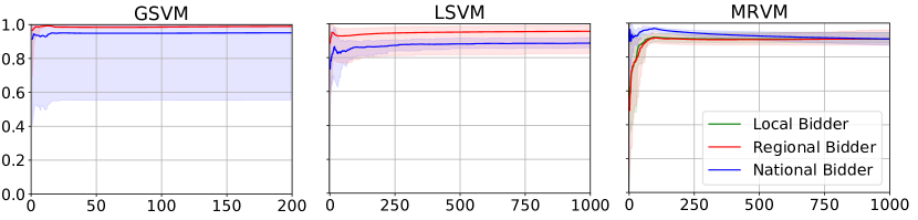
Figure 3: Average energy ratio (y-axis) with 97.5% and 2.5% empirical quantiles for a number of selected frequencies $k$ (x-axis) over 30 instances in GSVM and LSVM and over 5 instances in MRVM.

6.3 Efficiency Experiments

We now evaluate the efficiency of Hybrid Ica vs Mlca.

Results. Table 5 contains our main results in all domains. We show efficiency, distribution of efficiency to bidder types, revenue ${\scriptsize(\sum_{i\in N}p(R)_{i})/V(a^{*})}$, and runtime. First, we see that Hybrid Ica statistically significantly outperforms Mlca w.r.t. efficiency in GSVM and MRVM and performs on par in LSVM. Second, it also leads to a computational speedup ($\times 6$ GSVM, $\times 3$ LSVM, $\times 2$ MRVM). The reason for this computational speedup is that the generation of the $\ell_{3}+\ell_{4}$ Fourier queries (estimating the superset of the support using RWHT on the NNs, fitting the FT models using compressive sensing and solving our new FT-based MIPs) is faster than the generation of the NN-based MLCA allocation queries (training NNs and solving the NN-based MIP). Third, it distributes the welfare more evenly (= fairer) to bidder types. This also leads to a distribution that more closely resembles that of the efficient allocation (see Efficient Allocation). We present full efficiency path plots for the different phases of Hybrid Ica in Section D.3.

Fourier queries. To verify the importance of the $\ell_{3}$ Fourier reconstruction and $\ell_{4}$ Fourier allocation queries, we also present Hybrid Ica (no FR) and Hybrid Ica (no FR/FA), which use random queries in place of the $\ell_{3}$ Fourier reconstruction and the $\ell_{3}+\ell_{4}$ Fourier-based queries. As we see in Table 5, using the Fourier queries leads to significantly better efficiency and Hybrid Ica (no FR/FA) does not achieve a fairer efficiency distribution. A comparison of Hybrid Ica to Hybrid Ica (no FR) reveals that, in GSVM and LSVM, the Fourier reconstruction queries cause the fairer distribution. We empirically verified that these queries are composed of larger bundles (on avg. $17$ items vs. $4$ in MLCA queries) and thus allocate large bundles to bidders that would have been overlooked. In MRVM, the optimal query split for Hybrid Ica uses $\ell_{3}=0$ Fourier reconstruction queries such that Hybrid Ica is equal to Hybrid Ica (no FR). Thus, in MRVM, Hybrid Ica’s increased efficiency and fairer distribution results from the Fourier allocation queries.

Overall, we see that our Fourier-based auction is especially powerful in sparse domains. In practice, bidders are often limited by their cognitive abilities Scheffel et al. (2012) or use a low-dimensional computational model to represent their value function. Thus, their reported preferences typically exhibit only a limited degree of substitutability and complementarity, which is captured well by Fourier-sparsity.

7 Conclusion

We have introduced Fourier analysis for the design of CAs. The main idea was to represent value functions using Fourier-sparse approximations, providing us with a new lens on bidder’s values in the Fourier domain.

On a technical level, we have derived succinct MIPs for the Fourier transform-based WDPs, which makes computing Fourier-based allocation queries practically feasible. We have leveraged this to design a new hybrid ICA that uses NN and Fourier-queries. Our experiments have shown that our approach leads to higher efficiency, a computational speedup and a fairer distribution of social welfare than state-of-the-art.

With this paper, we have laid the foundations for future work leveraging Fourier analysis for representing and eliciting preferences in combinatorial settings.

Appendix

Appendix A Preliminaries

A.1 A Machine Learning powered ICA

In this section, we provide a detailed review of the machine learning-powered combinatorial auction (MLCA) introduced by Brero et al. Brero et al. [2021]. We describe MLCA using NNs $\mathcal{N}_{i}$ as the generic ML algorithm $\mathcal{A}_{i}$ (see Weissteiner and Seuken [2020]).

At the core of MLCA is a query module (Algorithm 2), which, for each bidder $i\in I$, determines a new value query $q_{i}$. First, in the estimation step (Line 1), NNs are used to learn bidders’ valuations from reports $R_{i}$. Next, in the optimization step (Line 2), a NN-based WDP is solved to find a candidate $q$ of value queries (see Weissteiner and Seuken [2020] for details on the NN-based estimation and optimization step). Finally, if $q_{i}$ has already been queried before (Line 4), another, more restricted NN-based WDP (Line 6) is solved and $q_{i}$ is updated correspondingly. This ensures that all final queries $q$ are new.

Function :  NextQueries$(I,R)$

Inputs :  Index set of bidders $I$ and reported values $R$

Parameters :  Neural networks $\mathcal{N}_{i}:\mathcal{X}\to\mathbb{R}_{+},\,i\in N$

1 foreach $i\in I$ do  Fit $\mathcal{N}_{i}$ on $R_{i}$: $\mathcal{N}_{i}[R_{i}]$

  $\triangleright$ Estimation step Solve $q\in\operatorname*{argmax}\limits_{a\in{\mathcal{F}}}\sum\limits_{i\in I}\mathcal{N}_{i}[R_{i}](a_{i})$

  $\triangleright$ Optimization step

2 foreach $i\in I$ do

3       if $q_{i}\in R_{i}$ then $\triangleright$ Bundle already queried

4             Define $\mathcal{F}^{\prime}=\{a\in\mathcal{F}:a_{i}\neq x,\forall x\in R_{i}\}$

5             Re-solve $q^{\prime}\in\operatorname*{argmax}_{a\in\mathcal{F}^{\prime}}\sum_{l\in I}\mathcal{N}_{l}{}[R_{l}](a_{l})$

6             Update $q_{i}=q^{\prime}_{i}\;$

return profile of new queries $q=(q_{1},\ldots,q_{n})$

Algorithm 2 NN-Query Module  (Brero et al. 2021)

Params : $t=1,Q^{\textrm{\tiny init}},Q^{\textrm{\tiny max}}$ init. and max #queries per bidder

1 foreach $i\in N$ do

2      Receive reports $R_{i}$ for $Q^{\textrm{\tiny init}}$ randomly drawn bundles

3while $t\leq\lfloor(Q^{\textrm{\tiny max}}-Q^{\textrm{\tiny init}})/n\rfloor$ do $\triangleright$ Round iterator

       $q^{\textrm{\tiny new}}=$ NextQueries$(N,R)$

        $\triangleright$ Main economy queries

4       foreach bidder $i\in N$ do $\triangleright$ Marginal economy queries

5             $q^{\textrm{\tiny new}}=q^{\textrm{\tiny new}}\cup$ NextQueries$(N\setminus\{i\},R_{-i})$

6      foreach bidder $i\in N$ do

7             Receive reports $R^{\textrm{\tiny new}}_{i}$ for $q^{\textrm{\tiny new}}_{i}$, set $R_{i}=R_{i}\cup R^{\textrm{\tiny new}}_{i}$

8      $t=t+1$

9From elicited reports $R$ compute $a^{*}_{R}$ as in Equation 1

10 From elicited reports $R$ compute VCG-payments $p(R)$

return Final allocation $a^{*}_{R}$ and payments $p(R)$

Algorithm 3 Mlca  (Brero et al. 2021)

In Algorithm 3, we present Mlca in a slightly abbreviated form. Let $R_{-i}=(R_{1},\ldots,R_{i-1},R_{i+1},\ldots,R_{n})$. Mlca proceeds in rounds until a maximum number of queries per bidder $Q^{\textrm{\tiny max}}$ is reached. In each round, it calls Algorithm 2 $n+1$ times: once including all bidders (Line 4, main economy) and $n$ times excluding one bidder (Lines 5–6, marginal economies). At the end of each round, the mechanism receives reports $R^{\textrm{\tiny new}}$ from all bidders for the newly generated queries $q^{\textrm{\tiny new}}$, and updates the overall elicited reports $R$ (Lines 7–8). In Lines 10–11, Mlca computes an allocation $a^{*}_{R}$ that maximizes the reported social welfare and determines VCG payments $p(R)$ (see Section A.2).

A.2 VCG Payments from Reports

In this section, we provide a recap on how to compute VCG payments from bidder’s reports. Let $R=(R_{1},\ldots,R_{n})$ denote an elicited set of reported bundle-value pairs from each bidder obtained from Mlca (Algorithm 3) or Hybrid Ica (Algorithm 1) and let $R_{-i}\coloneqq(R_{1},\ldots,R_{i-1},R_{i+1},\ldots,R_{n})$. We then calculate the VCG payments $p(R)=(p(R)_{1}\ldots,p(R)_{n})\in\mathbb{R}_{+}^{n}$ as follows:

Definition 2.

(VCG Payments from Reports)

$$p(R)_{i}\coloneqq\sum_{j\in N\setminus\{i\}}\hat{v}_{j}\left(\left(a^{*}_{R_{-i}}\right)_{j}\right)-\sum_{j\in N\setminus\{i\}}\hat{v}_{j}\left(\left(a^{*}_{R}\right)_{j}\right).$$ (22)

where $a^{*}_{R_{-i}}$ maximizes the reported social welfare when excluding bidder $i$, i.e.,

$$a^{*}_{R_{-i}}\in\operatorname*{argmax}_{a\in\mathcal{F}}\widehat{V}(a|R_{-i})=\operatorname*{argmax}_{a\in\mathcal{F}}\sum_{\begin{subarray}{c}j\in N\setminus\{i\}:\\ \left(a_{j},\hat{v}_{j}(a_{j})\right)\in R_{j}\end{subarray}}\hat{v}_{j}(a_{j}),$$ (23)

and $a^{*}_{R}$ is a reported-social-welfare-maximizing allocation (including all bidders), i.e,

$$a^{*}_{R}\in\operatorname*{argmax}_{a\in\mathcal{F}}\widehat{V}(a|R)=\operatorname*{argmax}_{a\in\mathcal{F}}\sum_{\hskip 28.45274pti\in N:\,\left(a_{i},\hat{v}_{i}(a_{i})\right)\in R_{i}}\hat{v}_{i}(a_{i}).$$ (24)

As argued by Brero et al. Brero et al. [2021], using such payments are key for Mlca to induce “good” incentives for bidders to report truthfully. As their incentive analysis also applies to Hybrid Ica, we use them in our design too.

Appendix B Fourier Transform-based WDPs

In this section, we present the proofs of Lemma 1 and Theorem 1.

Let $1_{d}$ and $0_{d}$ for $d\in\mathbb{N}$ denote the $d$-dimensional vector of ones and zeros, respectively. For all $x,y\in\mathbb{R}^{d},$ let $x\leq y,\,\max(x,y),\,\min(x,y)$ and $\left(-1\right)^{x}$ be defined component-wise, and let $\langle\cdot,\cdot\rangle$ denote the Euclidean scalar product.

We consider the matrix representation $F$ and $F^{-1}$ of the considered FTs from Püschel and Wendler Püschel and Wendler [2020] given by:

FT3: $$F_{y,x}=(-1)^{|y|-|x|}\mathbb{I}_{\min(x,y)=x},$$ (25)

$$F^{-1}_{x,y}=\mathbb{I}_{\min(x,y)=y},$$ (26)

FT4: $$F_{y,x}=(-1)^{|\min(x,y)|}\mathbb{I}_{\max(x,y)=1_{m}},$$ (27)

$$F^{-1}_{x,y}=\mathbb{I}_{\min(x,y)=0_{m}},$$ (28)

WHT: $$F_{y,x}=\frac{1}{2^{m}}(-1)^{|\min(x,y)|},$$ (29)

$$F^{-1}_{x,y}=(-1)^{|\min(x,y)|}.$$ (30)

The Fourier-sparse approximations used in the WDPs are defined in terms of $F^{-1}$.

B.1 Proof of Lemma 1

Lemma 1.

(Succinct Representations) For $i\in N$ let $\mathcal{S}_{i}=\{y^{(1)},\dots,y^{(k)}\}$ be the support of a $k$-Fourier-sparse approximation $\tilde{v}_{i}$ and $W_{i}\in\{0,1\}^{k\times m}$ be defined as $\left(W_{i}\right)_{l,j}=\mathbb{I}_{y^{(l)}_{j}=1}$. Then $\tilde{v}_{i}$ can be rewritten as:

FT3: $$\tilde{v}_{i}(x)=\left\langle\phi_{\tilde{v}_{i}|\mathcal{S}_{i}},\max\left(0_{k},1_{k}-W_{i}(1_{m}-x)\right)\right\rangle$$ (31)

FT4: $$\tilde{v}_{i}(x)=\left\langle\phi_{\tilde{v}_{i}|\mathcal{S}_{i}},\max\left(0_{k},1_{k}-W_{i}x\right)\right\rangle$$ (32)

WHT: $$\tilde{v}_{i}(x)=\left\langle\phi_{\tilde{v}_{i}|\mathcal{S}_{i}},(-1)^{W_{i}x}\right\rangle.$$ (33)

Proof.

In this proof we are going to make use of the equivalence between bundles (= indicator vectors) and sets. Recall that $x,y\in\mathcal{X}=\{0,1\}^{m}$ are bundles and bundles correspond to subsets of items. We can translate set operations such as intersection, union and complement to indicator vectors as follows:

$$x\cap y=\min(x,y),$$ (34)

$$x\cup y=\max(x,y),$$ (35)

$$(x)^{c}=1_{m}-x,$$ (36)

where we slightly abused notation by identifying the indicator vectors with their corresponding subsets on the left hand sides of (34)–(36). Furthermore, it holds that:

$$|\min(x,y)|=y^{T}x=\sum_{i=1}^{m}x_{i}y_{i}$$ (37)

FT3. Let $F$ denote the matrix representation of FT3 in (25). By definition, we have

$$\tilde{v}_{i}(x)= \sum_{y\in\mathcal{S}_{i}}F^{-1}_{x,y}\phi_{\tilde{v}_{i}}(y)$$ (38)

$$= \sum_{y\in\mathcal{S}_{i}}\mathbb{I}_{\min(x,y)=y}\phi_{\tilde{v}_{i}}(y)$$ (39)

$$= \sum_{y\in\mathcal{S}_{i}}\mathbb{I}_{\min(1_{m}-x,y)=0_{m}}\phi_{\tilde{v}_{i}}(y)$$ (40)

$$= \langle(\mathbb{I}_{\min(1_{m}-x,y)=0_{m}})_{y\in\mathcal{S}_{i}},\phi_{\tilde{v}_{i}|\mathcal{S}_{i}}\rangle,$$ (41)

where we used $x\cap y=y\Leftrightarrow x^{c}\cap y=\emptyset$. Now, the claim follows by observing that

$$\mathbb{I}_{\min(1_{m}-x,y)=0_{m}}=\max\left(0,1-y^{T}(1_{m}-x\right)),$$ (42)

which is a direct consequence of $|\min(1_{m}-x,y)|=y^{T}(1_{m}-x)$, and recalling that for each $y\in\mathcal{S}_{i}$ there is a respective row $y^{T}$ in $W_{i}$.

FT4. Let $F$ be the matrix representation of FT4 in (27). By definition, we have

$$\tilde{v}_{i}(x)= \sum_{y\in\mathcal{S}_{i}}F^{-1}_{x,y}\phi_{\tilde{v}_{i}}(y)$$ (43)

$$= \sum_{y\in\mathcal{S}_{i}}\mathbb{I}_{\min(x,y)=0_{m}}\phi_{\tilde{v}_{i}}(y)$$ (44)

$$= \langle(\mathbb{I}_{\min(x,y)=0_{m}})_{y\in\mathcal{S}_{i}},\phi_{\tilde{v}_{i}|\mathcal{S}_{i}}\rangle.$$ (45)

Now, the claim follows by observing that

$$\mathbb{I}_{\min(x,y)=0_{m}}=\max\left(0,1-y^{T}x\right),$$ (46)

which is a direct consequence of $|\min(x,y)|=y^{T}x$, and recalling that for each $y\in\mathcal{S}_{i}$ there is a respective row $y^{T}$ in $W_{i}$.

WHT. Let $F$ be the matrix representation of WHT in (29). By definition, we have

$$\tilde{v}_{i}(x)= \sum_{y\in\mathcal{S}_{i}}F^{-1}_{x,y}\phi_{\tilde{v}_{i}}(y)$$ (47)

$$= \sum_{y\in\mathcal{S}_{i}}(-1)^{y^{T}x}\phi_{\tilde{v}_{i}}(y)$$ (48)

$$= \langle((-1)^{y^{T}x})_{y\in\mathcal{S}_{i}},\phi_{\tilde{v}_{i}|\mathcal{S}_{i}}\rangle.$$ (49)

Now, the claim follows by recalling that for each $y\in\mathcal{S}_{i}$ there is a respective row $y^{T}$ in $W_{i}$. ∎

B.2 Proof of Theorem 1

We first state and proof two elementary lemmata.

For $x\in\mathbb{R}^{d}$ let $x\ (\mathrm{mod}\ 2)$ be defined component-wise.

Lemma 2.

(Max Representation) Let $\zeta,\eta\in\mathbb{R}^{d}$ for $d\in\mathbb{N}$ and $C>0$ such that for all $l\in\{1,\ldots,d\}$ it holds that $|\zeta_{l}-\eta_{l}|\leq C$. Let $\alpha:=\max(\zeta,\eta)$ and consider the polytope $\mathcal{P}$ in $(\tilde{\alpha},\beta)$ defined by (50)–(54)

$$\tilde{\alpha}\geq\eta$$ (50)

$$\tilde{\alpha}\leq\eta+C\beta$$ (51)

$$\tilde{\alpha}\geq\zeta$$ (52)

$$\tilde{\alpha}\leq\zeta+C(1_{d}-\beta)$$ (53)

$$\beta\in\{0,1\}^{d}.$$ (54)

Then it holds that $\mathcal{P}\neq\emptyset$ and every element $(\tilde{\alpha},\beta)\in\mathcal{P}$ satisfies $\tilde{\alpha}=\alpha.$

Proof.

Non-emptiness follows from the assumption that $|\zeta_{l}-\eta_{l}|\leq C$ for all $l\in\{1,\ldots,d\}$. For any $l\in\{1,\ldots,d\}$ we have to distinguish the following cases:

$$\zeta_{l}<\eta_{l}\implies\beta_{l}=0,\,\tilde{\alpha}_{l}=\eta_{l}=\max(\zeta_{l},\eta_{l})=\alpha_{l}$$

$$\zeta_{l}>\eta_{l}\implies\beta_{l}=1,\,\tilde{\alpha}_{l}=\zeta_{l}=\max(\zeta_{l},\eta_{l})=\alpha_{l}$$

$$\zeta_{l}=\eta_{l}\implies\tilde{\alpha}_{l}=\zeta_{l}=\eta_{l}=\max(\zeta_{l},\eta_{l})=\alpha_{l}$$

This yields that $\tilde{\alpha}=\alpha$. ∎

Lemma 3.

(Odd-Even Representation) Let $\zeta\in\mathbb{Z}^{d}$ for $d\in\mathbb{N}$. Let $\beta:=\zeta\ (\mathrm{mod}\ 2)\in\{0,1\}^{d}$ and consider the polytope $\mathcal{P}$ in $(\tilde{\beta},\gamma)$ defined by (55) and (56)

$$\tilde{\beta}=\zeta-2\gamma$$ (55)

$$\tilde{\beta}\in\{0,1\}^{d},\gamma\in\mathbb{Z}^{d}.$$ (56)

Then it holds that $\mathcal{P}\neq\emptyset$ and every element $(\tilde{\beta},\gamma)\in\mathcal{P}$ satisfies $\tilde{\beta}=\beta.$

Proof.

Non-emptiness follows since $\zeta\in\mathbb{Z}^{d}$ per assumption. For any $l\in\{1,\ldots,d\}$ we have to distinguish the following cases:

$$\zeta_{l}\ (\mathrm{mod}\ 2)=0\implies\gamma_{l}=\frac{\zeta}{2},\,\tilde{\beta}_{l}=0=\beta_{l}$$

$$\zeta_{l}\ (\mathrm{mod}\ 2)=1\implies\gamma_{l}=\frac{\zeta-1}{2},\,\tilde{\beta}_{l}=1=\beta_{l}$$

Thus $\tilde{\beta}=\beta$. ∎

For each bidder $i\in N$ let $\tilde{v}_{i}:\mathcal{X}\to\mathbb{R}_{+}$ be a Fourier-sparse approximation of the bidder’s reported value function $\hat{v}_{i}$. Then the Fourier transform-based WDP was defined as follows:

Definition 3.

(Fourier transform-based WDP)

$$\operatorname*{argmax}\limits_{a\in\mathcal{F}}\sum_{i\in N}\tilde{v}_{i}(a_{i}).$$ (FT-WDP)

Next, we proof Theorem 1.

Theorem 1.

(Fourier Transform-based MIPs) Let $\tilde{v}_{i}:\mathcal{X}\to\mathbb{R}$ be a k-Fourier-sparse approximation as defined in (31), (32), or (33). Then there exists a constant $C>0$ such that the MIP defined by the following objective

$$\operatorname*{argmax}\limits_{a\in\mathcal{F},\beta_{i}\in\{0,1\}^{k}}\sum_{i\in N}\langle\phi_{\tilde{v}_{i}|\mathcal{S}_{i}},\alpha_{i}\rangle,$$ (57)

and for $i\in N$ one set of transform specific constraints (58)–(60), or (61)–(63), or (64)–(66), is equivalent to (FT-WDP).

FT3:s.t. $$\alpha_{i}\geq 1_{k}-W_{i}(1_{m}-a_{i})$$ (58)

$$\alpha_{i}\leq 1_{k}-W_{i}(1_{m}-a_{i})+C\beta_{i}$$ (59)

$$0_{k}\leq\alpha_{i}\leq C(1_{k}-\beta_{i})$$ (60)

FT4:s.t. $$\alpha_{i}\geq 1_{k}-W_{i}a_{i}$$ (61)

$$\alpha_{i}\leq 1_{k}-W_{i}a_{i}+C\beta_{i}$$ (62)

$$0_{k}\leq\alpha_{i}\leq C(1_{k}-\beta_{i})$$ (63)

WHT:s.t. $$\alpha_{i}=-2\beta_{i}+1_{k}$$ (64)

$$\beta_{i}=W_{i}a_{i}-2\gamma_{i}$$ (65)

$$\gamma_{i}\in\mathbb{Z}^{k}$$ (66)

Proof.

We proof the equivalence for each of the FTs and corresponding MIPs separately.

• FT3
  Let $C>0$ such that $|\left[1_{k}-W_{i}(1_{m}-a_{i})\right]_{l}|\leq C$ for all $l\in\{1,\ldots,k\},i\in N$, and $a\in\mathcal{F}$. We then define

  $$\alpha_{i}:=\max\left(0_{k},1_{k}-W_{i}(1_{m}-a_{i})\right)\,\,\textrm{for all }i\in N,$$

  and apply for each $\alpha_{i}$ Lemma 2 to $\zeta:=0_{k}$ and ${\eta:=1_{k}-W_{i}(1_{m}-a_{i})}$, which concludes the proof for FT3.
  

• FT4:
  This follows analogously as for the FT3 when defining $\alpha_{i}:=\max(0_{k},1_{k}-W_{i}a_{i}),\,\zeta:=0_{k}$ and $\eta:=1_{k}-W_{i}a_{i}$.
  

• WHT:
  Since for all $i\in N$ and $a\in\mathcal{F}$ it holds that $W_{i}a_{i}\in\mathbb{Z}^{k}$, an immediate consequence from Lemma 3 is that $\beta_{i}=W_{i}a_{i}\ (\mathrm{mod}\ 2)$ and $(-1)^{W_{i}a_{i}}=-2\beta_{i}+1_{k}$, which concludes the proof for the WHT.

∎

Appendix C Analyzing the Potential of a FT-based CA

C.1 Fourier Sparsity - GSVM and MRVM

In this section, we provide the Fourier sparsity results for GSVM and MRVM. In Figure 4, we present the mean over 30 GSVM instances and bidder types. Figure 4 shows that GSVM is low degree $\leq 2$ in all considered FTs and thus can be represented using less or equal to $172=\binom{18}{0}+\binom{18}{1}+\binom{18}{2}$ FCs with any FT.

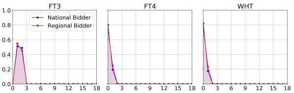
Figure 4: Spectral energy distribution in GSVM for different notions of FTs. For each cardinality (x-axis), we collect the spectral energy (y-axis) of all frequencies of that cardinality and normalize by the total spectral energy.

To the best of our knowledge it is not possible to compute the exact FCs with respect to any of the considered FTs for all MRVM bidders (see Wendler et al. [2021]). In Figure 5, we thus depict the approximate WHT-energy-distribution for MRVM. In order to do so, we used the RWHT algorithm by Amrollahi et al. Amrollahi et al. [2019], which recovers the largest WHT-FCs with high probability. Note that here we do not normalize by the total energy since the total energy is an unknown quantity in the space of $2^{98}$ bundles.

Figure 5 shows the approximate WHT-energy-distribution for MRVM. We see that while most of the energy is contained in the low degree FCs $\leq 2$, there is still some non negligible energy in the FCs of degree 3–7.

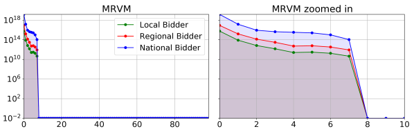
Figure 5: Approximate spectral energy distribution in MRVM for WHT computed with the robust WHT algorithm from Amrollahi et al. [2019]. For each cardinality (x-axis), we collect the spectral energy (y-axis) of all frequencies of that cardinality.

C.2 Reconstruction Error of Fourier Transforms

Using Procedure C.2, we determine the best $k$-Fourier-sparse approximation $\tilde{v}_{i}$ for all considered FTs.

(Best FCs Given Full Access to $\hat{v}_{i}$) 
Compute all FCs by using the full FT for each bidders’ reported value function $\phi_{\hat{v}_{i}}=F\hat{v}_{i}$. Next, compute $\tilde{v}_{i}$ by determining the $k$ best FCs $\phi_{\tilde{v}_{i}|\mathcal{S}_{i}}$ in terms of L2 error $\|\hat{v}_{i}-\tilde{v}_{i}\|_{2}^{2}$ as follows:

1. WHT: use the FCs of $\phi_{\hat{v}_{i}}$ with the $k$ largest absolute values.

2. FT3 and FT4: use the FCs with the $k$ largest coefficients $|\phi_{\hat{v}_{i}}(y)|\|F^{-1}_{\cdot,y}\|_{2}$, where $F^{-1}_{\cdot,y}$ denotes the $y$^th column.

In the following, we present the technical details for i. and ii. in Procedure C.2.

Let $F$ denote the corresponding matrix representation of the FT3, FT4, or the WHT. Furthermore, fix bidder $i\in N$ and for $\mathcal{S}_{i}\subseteq\operatorname*{supp}(\phi_{\hat{v}_{i}}),\,|\mathcal{S}_{i}|=k\ll 2^{m}$ let

$$\tilde{v}_{i}=\sum_{y\in\mathcal{S}_{i}}F^{-1}_{x,y}\phi_{\hat{v}_{i}}(y)=F^{-1}_{\cdot,\mathcal{S}_{i}}\phi_{\hat{v}_{i}|\mathcal{S}_{i}},$$

be a $k$-Fourier-sparse approximation, where we denote by $F^{-1}_{\cdot,\mathcal{S}_{i}}$ the sub matrix of $F^{-1}$ obtained by selecting the columns indexed by the bundles in $\mathcal{S}_{i}$.

C.2.1 Best Fourier Coefficients WHT

For the WHT, we consider the following optimization problem of selecting the $k$-best FCs with respect to the quadratic error:

$$\mathcal{S}_{i}^{*}\in\operatorname*{argmin}\limits_{\mathcal{S}_{i}\subseteq\operatorname*{supp}(\phi_{\hat{v}_{i}}),\,|\mathcal{S}_{i}|=k}\|\hat{v}_{i}-F^{-1}_{\cdot,\mathcal{S}_{i}}\phi_{\hat{v}_{i}|\mathcal{S}_{i}}\|_{2}^{2}.$$ (67)

Then, it follows that $\mathcal{S}_{i}^{*}$ consists out of those bundles $\{y^{(l)}\}_{l=1}^{k}$ with the largest absolute value of the corresponding FCs $\{\phi_{\hat{v}_{i}}(y^{(l)})\}_{l=1}^{k}$. This can be seen as follows.

$$\|\hat{v}_{i}-\underbrace{F^{-1}_{\cdot,\mathcal{S}_{i}}\phi_{\hat{v}_{i}|\mathcal{S}_{i}}}_{\tilde{v}_{i}}\|_{2}^{2}=\|\sum_{y\not\in\mathcal{S}_{i}}F^{-1}_{\cdot,y}\phi_{\hat{v}_{i}}(y)\|_{2}^{2}=$$ (68)

$$= \sum_{x,y\not\in\mathcal{S}_{i}}\langle F^{-1}_{\cdot,x},F^{-1}_{\cdot,y}\rangle\phi_{\hat{v}_{i}}(x)\phi_{\hat{v}_{i}}(y)=$$ (69)

$$= \sum_{y\not\in\mathcal{S}_{i}}\phi_{\hat{v}_{i}}(y)^{2},$$ (70)

where in the last equality we used that $F^{-1}$ is an orthogonal matrix and thus its columns fulfill $\langle F^{-1}_{\cdot,x},F^{-1}_{\cdot,y}\rangle=\mathbb{I}_{x=y}$.

For the other non-orthogonal transforms FT3 and FT4, we use a heuristic based on the triangular inequality to select the $k$ “best” FCs, which we present next.

C.2.2 Best Fourier Coefficients FT3 and FT4

For FT3 and FT4, we use the triangular inequality

$$\|\hat{v}_{i}-\underbrace{F^{-1}_{\cdot,\mathcal{S}_{i}}\phi_{\hat{v}_{i}|\mathcal{S}_{i}}}_{\tilde{v}_{i}}\|_{2}\leq\sum_{y\not\in\mathcal{S}_{i}}|\phi_{\hat{v}_{i}}(y)|\|F^{-1}_{\cdot,y}\|_{2}$$

to get an upper bound of the quadratic error $\|\hat{v}_{i}-\tilde{v}_{i}\|_{2}^{2}$ and select the FCs with the $k$ largest coefficients $|\phi_{\hat{v}_{i}}(y)|\|F^{-1}_{\cdot,y}\|_{2}$, where $F^{-1}_{\cdot,y}$ denotes the $y$^th column of $F^{-1}$.

Appendix D A Practical Hybrid ICA Mechanism

D.1 Technical Details of Hybrid Ica

In this section, we provide the technical details for the implementation of Hybrid Ica. In particular, we explain in more detail the Fourier Transform-based procedures D.1.1–D.1.3.

D.1.1 Determining the best FCs of NN

(Best FCs of Neural Networks)

1. If $m\leq 29:$ calculate the full FT of the NNs and select the best FCs.

2. If $m>29:$ use sparse FT algorithms, i.e., RWHT for WHT and SSFT Wendler et al. [2021] for FT3 and FT4 to obtain the best FCs of the NNs.

Using Procedure D.1.1 we determine the best FCs of the NN estimates of each bidder. We distinguish the two cases:

• Small number of items: if the number of items is small enough, i.e., $m\leq 29$, we determine the best FCs (and associated locations $\mathcal{S}_{i}\subset\mathcal{X}$) of $\mathcal{N}_{i}$ for all FTs by computing its full Fourier transform $F\mathcal{N}_{i}=\phi_{\mathcal{N}_{i}}$ using the respective algorithms from Püschel and Wendler Püschel and Wendler [2020].

• Large number of items: if the number of items is too large, i.e., $m>29$, we cannot compute the full Fourier transform and thus require sparse FT algorithms to compute the locations of the best FCs. For the WHT, we can do so by using the robust sparse WHT algorithm (RWHT) by Amrollahi et al. Amrollahi et al. [2019]. For FT3 and FT4, we use the sparse set function Fourier transform (SSFT) algorithm by Wendler et al. Wendler et al. [2021]. Both algorithms compute Fourier-sparse approximations by only using queries from the corresponding set function (= a bidder’s value function), and thus do not require a representation of the exponentially large full set function.

• Best WHT FCs: for the WHT the best FCs are the ones with the largest absolute values (see Section C.2.1). We select the locations of the $\ell_{\textrm{\tiny superset}}$ best NN FCs, i.e., $|\mathcal{S}_{i}|=\ell_{\textrm{\tiny superset}}$. We do so because we are going to use the compressive sensing method by Stobbe and Krause Stobbe and Krause [2012], which only requires a superset of the support $\operatorname*{supp}(\phi_{\hat{v}_{i}})$, in Procedure D.1.3 to fit a Fourier-sparse approximations $\tilde{v}_{i}$ to the bidders’ reports $R_{i}$. In our experiments, we set $\ell_{\textrm{\tiny superset}}=2,000$ for all domains. Ideally, we would like to choose $\ell_{\textrm{\tiny superset}}$ as large as possible to ensure that the best NN FCs actually overlap with the best FCs of $\hat{v}_{i}$, however, there is a trade-off between the number of samples (and also running time) required by the compressive sensing method and the size of the support superset. We did not optimize this hyperparameter.

• Best FT3 and FT4 FCs: for the FT3 and FT4 we use a heuristic based on the triangular inequality to select the best FCs and their locations (see Section C.2.2). As neither FT3 nor FT4 are orthogonal or satisfy the restricted isometry property required by the compressive sensing method, we only take the best $\ell_{3}$ locations of NN FCs, i.e., $|\mathcal{S}_{i}|=\ell_{3}$.

Notice that the goal of Procedure D.1.1 is solely to determine a set of bundles $\mathcal{S}_{i}\subseteq\mathcal{X}$ that is likely to contain many of the dominant FCs of $\hat{v}_{i}$. This set $\mathcal{S}_{i}$ is then used to determine reconstructing queries $\tilde{\mathcal{S}}_{i}$.

D.1.2 Determining reconstruction queries

(Fourier Reconstruction Queries)

1. FT3 and FT4: use the sampling theorems by Püschel and Wendler Püschel and Wendler [2020] to determine queries for the bidders, i.e., bundles $\tilde{\mathcal{S}}_{i}\subseteq\mathcal{X}$, that enable a reconstruction of $\tilde{v}_{i}$.

2. WHT: use the same queries as for FT4.

We make use of the sampling theorems for FT3 and FT4 presented by Püschel and Wendler Püschel and Wendler [2020] to obtain reconstruction queries, i.e., queries that help obtaining a small reconstruction error $\|\hat{v}_{i}-\tilde{v}_{i}\|_{2}$. Our rationale here is that the queries given by the sampling theorem $\tilde{\mathcal{S}}_{i}$ would lead to $\|\hat{v}_{i}-\tilde{v}_{i}\|_{2}=0$ for $\operatorname*{supp}(\phi_{\hat{v}_{i}})=\mathcal{S}_{i}$. The sampling theorem by Püschel and Wendler Püschel and Wendler [2020] selects rows $\tilde{\mathcal{S}}_{i}$ such that $F^{-1}_{\tilde{\mathcal{S}}_{i},\mathcal{S}_{i}}$ is of full rank, because then (iff $\operatorname*{supp}(\phi_{\hat{v}_{i}})=\mathcal{S}_{i}$) the Fourier coefficients $\phi_{\tilde{v}_{i}|\mathcal{S}_{i}}$ are the solution of the linear system of equations ${\hat{v}_{i\mid\tilde{\mathcal{S}}_{i}}=F^{-1}_{\tilde{\mathcal{S}}_{i},\mathcal{S}_{i}}\phi_{\tilde{v}_{i}|\mathcal{S}_{i}}}$. In particular, the theorem yields

• FT3: $\tilde{\mathcal{S}}_{i}=\mathcal{S}_{i}$,

• FT4: $\tilde{\mathcal{S}}_{i}=\{1_{m}-y:y\in\mathcal{S}_{i}\}$.

For the WHT there is no sampling theorem and we use

$$\tilde{\mathcal{S}}_{i}=\{1_{m}-y:|\phi_{\mathcal{N}_{i}}(y)|\text{ is in the }\ell_{3}\text{ largest in }\mathcal{S}_{i}\}$$

as a heuristic to obtain reconstruction queries. Choosing $\tilde{\mathcal{S}}_{i}$ in that way empirically often leads to a full-rank submatrix $F^{-1}_{\tilde{\mathcal{S}}_{i},\mathcal{Z}}$ of the inverse WHT obtained by selecting the rows indexed by $\tilde{\mathcal{S}}_{i}$ and the columns indexed by $\mathcal{Z}$, where $\mathcal{Z}\subseteq\mathcal{S}_{i}$ are the locations of the $\ell_{3}$ in absolute value largest FCs in $\mathcal{S}_{i}$, i.e., $\mathcal{Z}:=\{y:|\phi_{\mathcal{N}_{i}}(y)|\text{ is in the }\ell_{3}\text{ largest in }\mathcal{S}_{i}\}$. If $F^{-1}_{\tilde{\mathcal{S}}_{i},\mathcal{Z}}$ is full rank and $\operatorname*{supp}(\phi_{\hat{v}_{i}})=\mathcal{Z}$, the Fourier coefficients $\phi_{\hat{v}_{i}\mid\mathcal{Z}}$ are the solution of the linear system of equations ${\hat{v}_{i\mid\tilde{\mathcal{S}}_{i}}=F^{-1}_{\tilde{\mathcal{S}}_{i},\mathcal{Z}}\phi_{\hat{v}_{i}\mid\mathcal{Z}}}$.

D.1.3 Fitting Fourier-sparse approximations

(Fit Fourier-sparse $\tilde{v}_{i}$ to Reports)

1. FT3 and FT4: solve the least squares problem defined by the best FCs and reports $R_{i}$.

2. WHT: use the compressive sensing method by Stobbe and Krause Stobbe and Krause [2012] defined by the best FCs and reports $R_{i}$.

Lastly, we need to fit our Fourier-sparse approximations $\tilde{v}_{i}$ with $\operatorname*{supp}(\phi_{\tilde{v}_{i}})=\mathcal{S}_{i}$ to the elicited reports $R_{i}\coloneqq\left\{\left(x^{(l)},\hat{v}_{i}(x^{(l)})\right)\right\}$. That is, we determine values $w\in\mathbb{R}^{|\mathcal{S}_{i}|}$ for the FCs of the Fourier-sparse approximation $\tilde{v}_{i}=F^{-1}_{\cdot,\mathcal{S}_{i}}w$.

• WHT: as already mentioned, for the WHT this is done using the compressive sensing method by Stobbe and Krause Stobbe and Krause [2012]. We calculate the full regularization path for the L1-regularization parameter $\lambda$ using the LARS method from Efron et al. Efron et al. [2004], and select the $\lambda$ that yields $\ell_{\textrm{\tiny support}}$ non zero FCs. In our experiments we set $\ell_{\textrm{\tiny support}}=100$ in GSVM and LSVM and $\ell_{\textrm{\tiny support}}=500$ in MRVM. We did not optimize this hyperparameter.

• FT3 and FT4: for FT3 and FT4 we cannot use the compressive sensing method and instead solve the following least squares problem

  $$\min_{w\in\mathbb{R}^{\ell_{3}}}\sum_{(x,\hat{v}_{i}(x))\in R_{i}}\left(\hat{v}_{i}(x)-\underbrace{\left(F^{-1}_{\cdot,\mathcal{S}_{i}}w\right)(x)}_{=\tilde{v}_{i}(x)}\right)^{2}.$$

In Figure 6, we present a flow diagram of the different algorithms we use in Hybrid Ica.

D.2 Details of NNs Support Discovery Experiments

In this section, we discuss the energy ratio plot (see Figure 3 in the main paper) for the large domain MRVM with $m=98$ items. Recall, that in MRVM one cannot compute the full FT analytically and one has to use sparse FT algorithms to obtain an approximation of the true $k$-best possible frequencies $\mathcal{S}_{i}^{*}=\{\overset{*}{y}{}^{(1)},\dots,\overset{*}{y}{}^{(k)}\}$. For this we use the recently developed RWHT algorithm from Amrollahi et al. Amrollahi et al. [2019], which computes the largest WHT-FCs with high probability and thus gives us an approximation $\mathcal{S}_{i}^{\text{rwht}}\approx\mathcal{S}_{i}^{*}$. As in the main paper, we then calculate for each bidder $i\in N$ the energy ratio of the support found by the corresponding NNs $\mathcal{\tilde{S}}_{i}$ and $\mathcal{S}_{i}^{\text{rwht}}$.

D.3 Details of Efficiency Experiments

In Figures 9–9, we present detailed efficiency results of Hybrid Ica in all three SATS domains, where we used the best found configuration of hyperparameters from Table 4 in the main paper.

In the upper plot we show in each figure the efficiency of the different phases of Hybrid Ica. In the lower plot, we present a histogram of the final efficiency distribution over 100 (in GSVM and LSVM) and 30 (in MRVM) new CA instances. To enable a head-to-head comparison, we use for the test set of CA instances the seeds 1–100 in GSVM and LSVM, and seeds 51–80 in MRVM.

All experiments were conducted on machines with Intel Xeon E5 v4 2.20GHz processors with 24 cores and 128GB RAM or with Intel E5 v2 2.80GHz processors with 20 cores and 128GB RAM.

D.3.1 GSVM (Figure 9)

After $30$ random queries, Hybrid Ica achieves an (avg.) efficiency of $66\%$. Next, after three Mlca iterations, i.e., $21$ MLCA queries, 99 instances have an efficiency $\geq 90\%$. Finally, the Fourier-based queries significantly increase the (avg.) efficiency by 1.87 percentage points from 98.1% to 99.97%.​​ Furthermore, we present in the lower plot a histogram of the final efficiency distribution. We see, that for 94 out of 100 instances Hybrid Ica impressively achieves an economic efficiency of 100% using in total only 100 value queries per bidder.

D.3.2 LSVM (Figure 9)

Starting with $\ell_{1}=30$ random initial queries, Hybrid Ica achieves an average efficiency of approximately $62\%$. Next, Hybrid Ica performs 5 Mlca iterations. After these 5 Mlca iterations, Hybrid Ica already found for each of the 100 instances an allocation with an efficiency of at least 80% with an average efficiency of 97.80%. Here, in the non-sparse LSVM domain, the Fourier reconstruction and allocation queries can increase the efficiency of some outliers arriving at an average efficiency of 98.74%. In the histogram, we see, that for 66 instances, Hybrid Ica was able to achieve full efficiency. Overall, we observe, that in the non-sparse LSVM the Fourier-based approach is not as effective as in the sparse GSVM, but still leads to results, that statistically match the efficiency of Mlca (see Table 5 in the main paper).

D.3.3 MRVM (Figure 9)

Starting with $\ell_{1}=30$ random initial queries, Hybrid Ica achieves an average efficiency of approximately $50\%$. Next, Hybrid Ica performs 55 Mlca iterations and asks in total 220 MLCA allocation queries. Here, we observe a steep increase in efficiency at the beginning. In later iterations the increase in efficiency gets smaller resulting in an average efficiency of $94.20\%$. In MRVM, the best query split we found uses $\ell_{3}=0$ Fourier-based reconstruction queries, thus the Fourier reconstruction queries (FR) do not change the efficiency distribution in Figure 9. However, the $\ell_{4}=250$ Fourier-based allocation queries significantly increase the efficiency further by $2.43\%$ resulting in a final average efficiency of $96.63\%$.

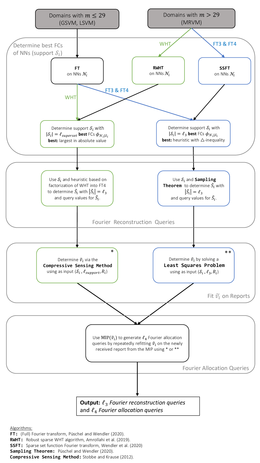
Figure 6: Overview of Fourier Transform-based Procedures in Hybrid Ica.

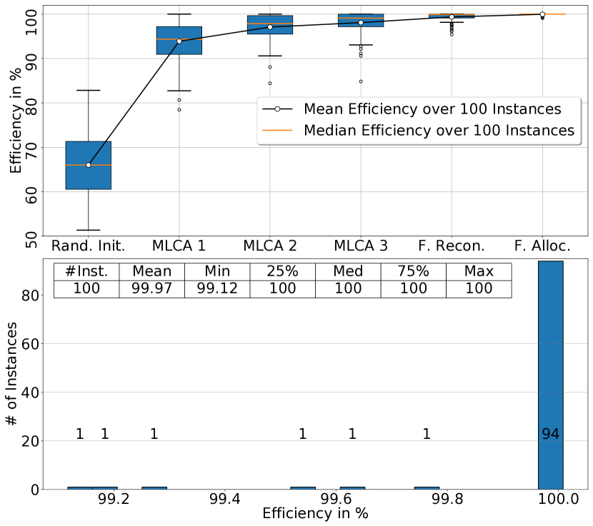
Figure 7: Details of Hybrid Ica in GSVM.

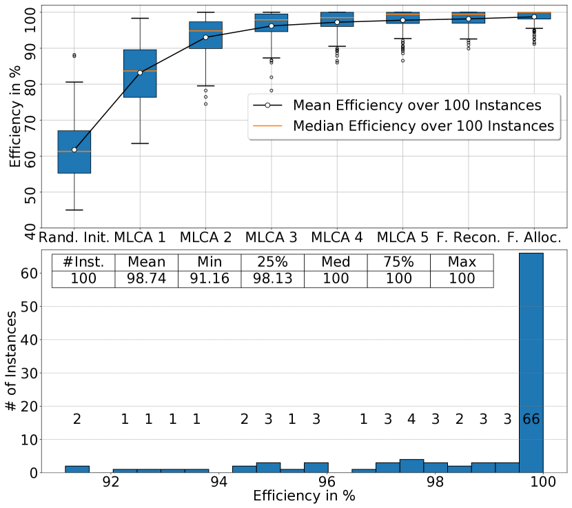
Figure 8: Details of Hybrid Ica in LSVM.

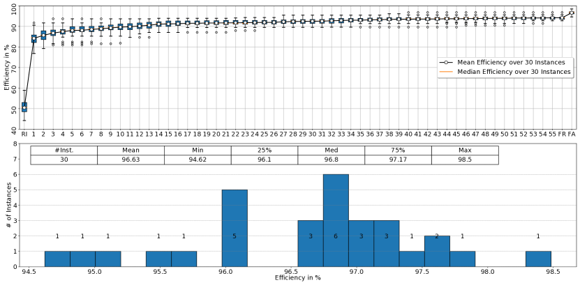
Figure 9: Details of Hybrid Ica in MRVM.

References

- Abraham et al. [2012] I. Abraham, M. Babaioff, S. Dughmi, and T. Roughgarden. Combinatorial auctions with restricted complements. In Proceedings of the 13th ACM Conference on Electronic Commerce, 2012.
- Amrollahi et al. [2019] A. Amrollahi, A. Zandieh, M. Kapralov, and A. Krause. Efficiently learning Fourier sparse set functions. In Advances in Neural Information Processing Systems, 2019.
- Ausubel and Baranov [2017] L. M. Ausubel and O. Baranov. A practical guide to the combinatorial clock auction. Economic Journal, 127(605):F334–F350, 2017.
- Ausubel and Cramton [2011] L. Ausubel and P. Cramton. Auction design for wind rights. Report to Bureau of Ocean Energy Management, Regulation and Enforcement, 2011.
- Ausubel et al. [2006] L. Ausubel, P. Cramton, and P. Milgrom. The clock-proxy auction: A practical combinatorial auction design. In Combinatorial Auctions, pages 115–138. MIT Press, 2006.
- Bernasconi et al. [1996] A. Bernasconi, B. Codenotti, and J. Simon. On the Fourier analysis of Boolean functions. preprint, pages 1–24, 1996.
- Blum et al. [2004] A. Blum, J. Jackson, T. Sandholm, and M. Zinkevich. Preference elicitation and query learning. Journal of Machine Learning Research, 5:649–667, 2004.
- Brero et al. [2018] G. Brero, B. Lubin, and S. Seuken. Combinatorial auctions via machine learning-based preference elicitation. In Proceedings of the 27th International Joint Conference on Artificial Intelligence, 2018.
- Brero et al. [2019] G. Brero, S. Lahaie, and S. Seuken. Fast iterative combinatorial auctions via bayesian learning. In Proceedings of the 33rd AAAI Conference of Artificial Intelligence, 2019.
- Brero et al. [2021] G. Brero, B. Lubin, and S. Seuken. Machine learning-powered iterative combinatorial auctions. arXiv preprint arXiv:1911.08042, Jan 2021.
- Cramton [2013] P. Cramton. Spectrum auction design. Review of Industrial Organization, 42(2):161–190, 2013.
- Dütting et al. [2019] P. Dütting, Z. Feng, H. Narasimhan, D. Parkes, and S. Ravindranath. Optimal auctions through deep learning. In Proceedings of the 36th International Conference on Machine Learning, 2019.
- Efron et al. [2004] B. Efron, T. Hastie, I. Johnstone, R. Tibshirani, et al. Least angle regression. The Annals of statistics, 32(2):407–499, 2004.
- Goeree and Holt [2010] J. K. Goeree and C. A. Holt. Hierarchical package bidding: A paper & pencil combinatorial auction. Games and Economic Behavior, 2010.
- Heiss et al. [2022] Jakob M Heiss, Jakob Weissteiner, Hanna S Wutte, Sven Seuken, and Josef Teichmann. NOMU: Neural optimization-based model uncertainty. In Proceedings of the 39th International Conference on Machine Learning, volume 162 of Proceedings of Machine Learning Research, pages 8708–8758. PMLR, 17–23 Jul 2022.
- Hudson and Sandholm [2003] B. Hudson and T. Sandholm. Using value queries in combinatorial auctions. In Proceedings of the 4th ACM Conference on Electronic commerce, pages 226–227, 2003.
- Lahaie and Parkes [2004] S. Lahaie and C. Parkes. Applying learning algorithms to preference elicitation. In Proceedings of the 5th ACM Conference on Electronic Commerce, 2004.
- Lahaie [2010] S. Lahaie. Kernel methods for revealed preference analysis. In ECAI, pages 439–444, 2010.
- Milgrom [2007] P. Milgrom. Package auctions and exchanges. Econometrica, 75(4):935–965, 2007.
- Nisan and Segal [2006] N. Nisan and I. Segal. The communication requirements of efficient allocations and supporting prices. Journal of Economic Theory, 2006.
- O’Donnell [2014] R. O’Donnell. Analysis of boolean functions. Cambridge University Press, 2014.
- Püschel and Wendler [2020] M. Püschel and C. Wendler. Discrete signal processing with set functions. IEEE Transactions on Signal Processing, 69:1039–1053, 2020.
- Rahaman et al. [2019] N. Rahaman, A. Baratin, D. Arpit, F. Draxler, M. Lin, F. Hamprecht, Y. Bengio, and A. Courville. On the spectral bias of neural networks. In International Conference on Machine Learning, 2019.
- Rahme et al. [2021] J. Rahme, S. Jelassi, J. Bruna, and M. Weinberg. A permutation-equivariant neural network architecture for auction design. In Proceedings of the 35th AAAI Conference on Artificial Intelligence, 2021.
- Scheffel et al. [2012] T. Scheffel, G. Ziegler, and M. Bichler. On the impact of package selection in combinatorial auctions: an experimental study in the context of spectrum auction design. Experimental Economics, 2012.
- Shen et al. [2019] W. Shen, P. Tang, and S. Zuo. Automated mechanism design via neural networks. In Proceedings of the 18th International Conference on Autonomous Agents and MultiAgent Systems, 2019.
- Shen et al. [2020] W. Shen, B. Peng, H. Liu, M. Zhang, R. Qian, Y. Hong, Z. Guo, Z. Ding, P. Lu, and P. Tang. Reinforcement mechanism design: With applications to dynamic pricing in sponsored search auctions. In Proceedings of the 34th AAAI Conference, 2020.
- Stobbe and Krause [2012] P. Stobbe and A. Krause. Learning Fourier sparse set functions. In Artificial Intelligence and Statistics, 2012.
- Weiss et al. [2017] M. Weiss, B. Lubin, and S. Seuken. Sats: A universal spectrum auction test suite. In Proceedings of the 16th Conference on Autonomous Agents and Multi-Agent Systems, 2017.
- Weissteiner and Seuken [2020] Jakob Weissteiner and Sven Seuken. Deep learning—powered iterative combinatorial auctions. Proceedings of the AAAI Conference on Artificial Intelligence, 34(02):2284–2293, Apr. 2020.
- Weissteiner et al. [2022a] Jakob Weissteiner, Jakob Heiss, Julien Siems, and Sven Seuken. Monotone-value neural networks: Exploiting preference monotonicity in combinatorial assignment. In Proceedings of the Thirty-First International Joint Conference on Artificial Intelligence, IJCAI-22, pages 541–548. International Joint Conferences on Artificial Intelligence Organization, 7 2022. Main Track.
- Weissteiner et al. [2022b] Jakob Weissteiner, Chris Wendler, Sven Seuken, Ben Lubin, and Markus Püschel. Fourier analysis-based iterative combinatorial auctions. In Proceedings of the Thirty-First International Joint Conference on Artificial Intelligence, IJCAI-22, pages 549–556. International Joint Conferences on Artificial Intelligence Organization, 7 2022. Main Track.
- Weissteiner et al. [2023] Jakob Weissteiner, Jakob Heiss, Julien Siems, and Sven Seuken. Bayesian optimization-based combinatorial assignment. Proceedings of the AAAI Conference on Artificial Intelligence, 37, 2023.
- Wendler et al. [2021] C. Wendler, A. Amrollahi, B. Seifert, A. Krause, and M. Püschel. Learning set functions that are sparse in non-orthogonal Fourier bases. In Proceedings of the 35th AAAI Conference on Artificial Intelligence, 2021.