Evolution of Non-Gaussian Hydrodynamic Fluctuations

Abstract

In the context of the search for the QCD critical point using non-Gaussian fluctuations, we obtain the evolution equations for non-Gaussian cumulants to the leading order of the systematic expansion in the magnitude of thermal fluctuations. We develop a diagrammatic technique in which the leading order contributions are given by tree diagrams. We introduce a Wigner transform for multipoint correlators and derive the evolution equations for three- and four-point Wigner functions for the problem of nonlinear stochastic diffusion with multiplicative noise.

I Introduction

The recent resurgence of interest in the classic subject of hydrodynamics in general Landau:2013fluid and hydrodynamic fluctuations Landau:2013stat2 in particular has been largely driven by the progress in heavy-ion collision experiments that create and study droplets of hot and dense matter governed by the physics of strong interactions described by quantum chromodynamics (QCD). The importance of fluctuations in heavy-ion collisions is due to the fact that the QCD fireballs created in such experiments, with typical particle multiplicities $\mathcal{O}(10^{2-4})$, while being large enough for hydrodynamics to apply, are not too large for fluctuations to be negligible.

Such fluctuations are observable in heavy-ion collisions via event-by-event measurements. Furthermore, fluctuations are enhanced if the matter created in the collisions is in a state close to a critical point and can serve as signatures of the criticality Stephanov:1998dy ; Stephanov:1999zu ; Stephanov:2008qz ; Stephanov:2011pb in the beam energy scan experiments Aggarwal:2010cw ; Bzdak:2019pkr . The magnitude of the signatures is determined by the competition between the critical slowing down and the finiteness of the expansion time Stephanov:1999zu ; Berdnikov:1999ph ; Mukherjee:2015swa ; Akamatsu:2018tcp .

This necessitates a quantitative description of the fluctuation evolution within a hydrodynamic framework, and there have been significant advances in that area recently Kapusta:2011gt ; Kapusta:2012zb ; Young:2014pka ; Stephanov:2018hydro+ ; Akamatsu:2017 ; Akamatsu:2018 ; Martinez:2018 ; Nahrgang:2018afz ; An:2019rhf ; An:2019fdc ; An:2020jjk ; Rajagopal:2019hydro ; Du:2020bxp ; Chao:2020kcf . Most relevant for this work is the formalism describing the evolution of correlation functions coupled to the hydrodynamic background. While the approach was considered long ago in a nonrelativistic context Andreev:1978 , the relativistic formalism has been introduced recently in the boost-invariant Bjorken flow characteristic of heavy-ion collisions in Refs. Akamatsu:2017 ; Akamatsu:2018 , and in general background in Refs. An:2019rhf ; An:2019fdc .

However, so far the formalism has been limited to two-point correlation functions. The description of the higher-point correlators quantifying the non-Gaussianity of the fluctuations has been elusive until now. On the other hand, the experimental search for the QCD critical point relies heavily on such measures of non-Gaussianity Stephanov:2008qz ; Stephanov:2011pb ; Bzdak:2019pkr ; Aggarwal:2010cw (which, similar to fluctuation magnitudes, depend on time evolution Mukherjee:2015swa ). We tackle this crucial gap between the ability of the theory w.r.t. non-Gaussian fluctuations and the demand of the experiment.

We obtain evolution equations for appropriate measures of non-Gaussianity in the hydrodynamic regime, that is, the regime where the ratio of correlation length to typical fluctuation wavelength is small. Such a regime exists even near the critical point, provided the correlation length remains much shorter than the size of the system, as is the case in most physical systems, including heavy-ion collisions.

II General multivariable formalism

To understand better the issues of nonlinearity and multiplicative noise, which is essential for non-Gaussian fluctuations, we begin with a more general formalism for a discrete set of stochastic variables $\breve{v}_{i}$, labeled by index $i$. The set of stochastic Langevin equations reads

$$\frac{d\breve{v}_{i}}{dt}=F_{i}[\breve{v}]+H_{ij}[\breve{v}]\eta_{j}\,,$$ (1)

where drift $F$ and noise magnitude $H$ are functions of $\breve{v}_{i}$, summation over repeated indices is implied, and $\eta_{i}$ is the Gaussian white noise, i.e.,

$$\langle\eta_{i}(t_{1})\eta_{j}(t_{2})\rangle=2\delta_{ij}\delta(t_{1}-t_{2}).$$ (2)

Eq. (1) suffers from a well-known ambiguity often referred to as the problem of multiplicative noise: it needs additional information to define the product of the stochastic function $H[\breve{v}]$ and the noise $\eta$. From our point of view, this is not really a problem but rather a shortcoming of the notation used in Eq. (1), which does not reflect the necessary information. The ambiguity is removed by discretizing time in Eq. (1) and taking the limit $\Delta t\to 0$. The choice of the definition of the product of $H$ and $\eta$ is a matter of convenience. We shall use the choice known as Ito calculus, where $H$ and $\eta$ are evaluated at the same moment. It is also well-known that the change of the definition of stochastic calculus (e.g., Stratonovich instead of Ito) is simply equivalent to a shift of the drift term $F_{i}$ ZinnJustin:2002ru .

Using Ito calculus, one can derive a Fokker-Plank equation for the probability distribution of $\breve{v}$:

$$\partial_{t}P=\left(-F_{i}P+\left(Q_{ij}P\right)_{,j}\right)_{,i},$$ (3)

where $Q\equiv HH^{T}$, $(\ldots)_{,i}\equiv\partial(\ldots)/\partial v_{i}$ and $\partial_{t}\equiv\partial/\partial t$. The Fokker-Plank equation is unambiguous as written, unlike the Langevin equation [Eq. (1)].

Let us consider the equilibrium solution $P_{\rm eq}$ to the Fokker-Plank equation, i.e., $\partial_{t}P_{\rm eq}=0$. While the divergence of the probability flux on the rhs of Eq. (3) vanishes, the flux itself does not have to and could be equal to the divergence of an antisymmetric 2-form, which we write as

$$F_{i}P_{\rm eq}-\left(Q_{ij}P_{\rm eq}\right)_{,j}=\left(\Omega_{ij}P_{\rm eq}\right)_{,j}\,,$$ (4)

where $\Omega_{ij}=-\Omega_{ji}$. Thus, $F_{i}$ can be expressed in terms of the equilibrium distribution

$$F_{i}=P_{\rm eq}^{-1}\left((Q+\Omega)_{ij}P_{\rm eq}\right)_{,j}=M_{ij}S_{,j}+M_{ij,j}\,,$$ (5)

where we introduced the Onsager matrix

$$M\equiv Q+\Omega\quad\mbox{and also}\quad S\equiv\log P_{\rm eq}\,.$$ (6)

Rather than defining the stochastic process in terms of the function $F_{i}$, which additionally needs specification of the stochastic calculus rule, it makes more sense to use $S$ and $M$ to define the process Arnold:1999uza . While $S$ describes the equilibrium distribution, and in a certain sense is analogous to entropy, the matrix $M$ describes the dynamics of the stochastic process: the symmetric semipositive definite part $Q$ is responsible for relaxation and the antisymmetric matrix $\Omega$ (symplectic form) for the Hamiltonian-like nondissipative motion. These physical properties of the process are independent of the stochastic calculus prescription, while their relationship to drift $F$ depends on such a prescription and is written in Eq. (5) for Ito calculus.

III Perturbative expansion

Using the Fokker-Plank equation [Eq. (3)], we can now write the evolution equation for any function of variables $\breve{v}$, including arbitrary products of their fluctuations $\delta v_{i}=\breve{v}_{i}-\langle{\breve{v}_{i}}\rangle$ or $n$-point functions such as $G_{i_{1}\ldots i_{n}}\equiv\langle{\delta v_{i_{1}}\ldots\delta v_{i_{n}}}\rangle\equiv G_{n}$.

For example, if $S$ is a bilinear function of $v_{i}$ and $M_{ij}$ are constants, (i.e., when Eq. (1) describes a linear Ornstein-Uhlenbeck process) the equations for $G_{n}$ are linear and involve only $G_{n}$ and $G_{n-2}$, and therefore can be solved iteratively. The equations for the cumulants,

$$G^{\text{c}}_{i_{1}\ldots i_{n}}\equiv\left.\frac{\partial^{n}\log\langle{\exp(\mu_{i}\breve{v}_{i})}\rangle}{\partial\mu_{i_{1}}\ldots\partial\mu_{i_{n}}}\right|_{\mu=0},$$ (7)

are even simpler — they decouple from each other. Equilibrium is achieved when all $n>2$ cumulants vanish, as expected for the Gaussian distribution $P_{\rm eq}=e^{S}$, while $G^{\rm eq}_{2}=-(S^{\prime\prime})^{-1}$ where $(S^{\prime\prime})_{ij}\equiv S_{,ij}$.

In general, $S$ is not a bilinear and $M_{ij}$ are not constants, and we have an infinite system of coupled equations for cumulants. To organize this system into a hierarchy, we develop a perturbation theory.

In many physical systems of interest, particularly in hydrodynamics, the fluctuations around the equilibrium are controllably small. In other words, the probability distribution $P$ is sharply peaked and can be treated as Gaussian in the lowest order of an approximation.

To be systematic, we introduce an expansion parameter $\varepsilon$ to control the magnitude of the deviations from equilibrium. We assume

$$S^{\prime\prime}\sim\varepsilon^{-1}$$ (8)

and that this remains true for all higher-order derivatives of $S$, ensuring that for small $\varepsilon$ the probability distribution $e^{S}$ approaches a narrow Gaussian with the characteristic magnitude of fluctuations $|\delta v|\sim\sqrt{G_{2}}\sim\sqrt{\varepsilon}$.

Thus, $G_{2n-1}\sim G_{2n}\sim\varepsilon^{n}.$ The odd-order moments $G_{2n-1}$ are of the same order as $G_{2n}$ because $\langle\delta v\rangle=0$. On the other hand, the non-Gaussian cumulants are smaller for the same order:

$$G^{\text{c}}_{n}\sim\varepsilon^{n-1}.$$ (9)

This power counting is easily established by a diagrammatic expansion of Eq. (7) using probability $e^{S}$, with $(S^{\prime\prime})^{-1}\sim\varepsilon$ playing the role of a propagator and each vertex being of order $\varepsilon^{-1}$.

Because, according to Eq. (9), cumulants of higher orders are progressively suppressed, the hierarchy is now parametrically controllable by $\varepsilon$. Truncating each equation at the leading order, we find, for $n=2,3$,

$$\partial_{t}G^{\text{c}}_{i_{1}i_{2}}=\left[{M}_{i_{1}j}\left(S_{,jk}G^{\text{c}}_{ki_{2}}+\delta_{ji_{2}}\right)\right]_{{\rm P}i_{1}i_{2}},$$ (10a)

$$\partial_{t}G^{\text{c}}_{i_{1}i_{2}i_{3}}=\Big{[}\frac{1}{2}{M}_{i_{1}j}\left(S_{,jk}G^{\text{c}}_{ki_{2}i_{3}}+S_{,jk\ell}G^{\text{c}}_{ki_{2}}G^{\text{c}}_{\ell i_{3}}\right)\\ +{M}_{i_{1}j,m}G^{\text{c}}_{mi_{2}}\left(S_{,jk}G^{\text{c}}_{ki_{3}}+\delta_{ji_{3}}\right)\Big{]}_{{\rm P}i_{1}i_{2}i_{3}},$$ (10b)

where $[\ldots]_{{\rm P}i_{1}\ldots i_{n}}$ denotes the sum over permutations of indices. The corresponding equation for $\partial_{t}G^{\text{c}}_{i_{1}i_{2}i_{3}i_{4}}$ contains nine terms (before index permutations), and it is easier to express using diagrammatic representation in Figs. 1 and 2. The symmetry factors, such as $1/2$ in Eq. (10b), count the number of permutations that do not produce different terms.

It is notable that the only diagrams appearing at the leading order in $\varepsilon$ are “trees.” The first term in each equation is the same as in the linear problem, as it involves only $S^{\prime\prime}$ and no derivatives of $M$. Other terms are due to nonlinearities and/or multiplicative noise, which contribute at the same order in $\varepsilon$. Higher-order terms contain loop diagrams, which we shall not discuss in this Letter.

In most applications, the noise $\eta$ is almost Gaussian, being a cumulative result of many uncorrelated factors. In our approach, one can treat noise non-Gaussianity systematically when $H$ is a small parameter and the noise cumulants obey the same hierarchy, as in Eq. (9). These assumptions hold in hydrodynamics. The $n$-th ($n>2$) noise cumulant contribution will enter at order $H^{n}$, while the leading terms we keep in Eq. (10) are of order $H^{2}$.

Figure 1: Diagrammatic notation used in Fig. 2 to represent the evolution equations [Eq. (10)]. The subsets of diagrams denoted by half-filled circles vanish in equilibrium.

Figure 2: Diagrammatic representation of the evolution equations [Eq. (10)] using notations described in Fig. 1.

Eq. (10) and its diagrammatic representation are among the main results of this work. We shall apply this approach to hydrodynamics, i.e., a system of stochastic continuum fields, rather than discrete variables.

IV Stochastic Nonlinear Diffusion

As the simplest example of a stochastic hydrodynamic problem, we shall consider the diffusion of conserved density (of, e.g., particle number or charge) in a slowly evolving (e.g., expanding and/or cooling) medium. This problem carries the most important features we want to address in this work, including multiplicative noise, without the complications of additional degrees of freedom and the Hamiltonian (nondissipative) dynamics of ideal fluid motion. We shall postpone the extension of these results to full stochastic hydrodynamics to future work but will discuss the implications of our findings below.

The diffusion equation is essentially a conservation equation for fluctuating density $\breve{n}$:

$$\partial_{t}\breve{n}=-\bm{\nabla}\cdot\bm{\breve{J}}\,,$$ (11a)

where the constitutive relation is

$$\bm{\breve{J}}=-\breve{\lambda}\bm{\nabla}\breve{\alpha}+\sqrt{\breve{\lambda}}\,\bm{\eta},$$ (11b)

with the stochastic noise $\bm{\eta}$ given by

$$\langle{\eta^{i}(t_{1},\bm{x})\,\eta^{j}(t_{2},\bm{y})}\rangle=2\delta^{ij}\delta(t_{1}-t_{2})\delta^{(3)}(\bm{x}-\bm{y}).$$ (12)

$\breve{\lambda}=\lambda(\breve{n})$ is conductivity and $\breve{\alpha}=\alpha(\breve{n})$ is chemical potential (in units of temperature).

To translate the generic multivariable stochastic system into a stochastic hydrodynamic diffusion problem, we use the following dictionary:

$$\delta_{ij} \to\delta^{(3)}(\bm{x}-\bm{y})\equiv\delta_{\bm{x}\bm{y}},~{}v_{i}\to n(\bm{x})\equiv n_{\bm{x}},$$ (13a)

$$S \to\int_{\bm{x}}\left(s(n_{\bm{x}})+\bar{\alpha}n_{\bm{x}}\right),$$ (13b)

$$S_{,i} \to{\delta S}/{\delta n_{\bm{x}}}=-(\alpha(n_{\bm{x}})-\bar{\alpha}),$$ (13c)

$${M}_{ij} \to-\bm{\nabla}_{\bm{x}}\lambda(n_{\bm{x}})\bm{\nabla}_{\bm{x}}\delta_{\bm{xy}},$$ (13d)

where $\alpha=-\partial s/\partial n$ and $\bar{\alpha}$ is a constant, understood as the chemical potential (in units of temperature) of the particle reservoir controlling the average particle density (similar to a Lagrange multiplier). Since the indices $i$, $j$, etc. become continuous coordinates $\bm{x}$, $\bm{y}$, etc., matrices $M$ and $H$ become operators, which in Eq. (13) are expressed in terms of their integral kernels. They are local, i.e., could be also written as differential operators, i.e., $H=\bm{\nabla}\sqrt{\lambda}$ and $M=-\bm{\nabla}\lambda\bm{\nabla}$. Note that ${M}=HH^{T}$, i.e., $\Omega=0$ for the diffusion problem.

As in Eq. (1), because the noise is multiplied by a function of the stochastic variable $\breve{n}$, the stochastic equation [Eq. (11)] is not well-defined as written. As before, we can define the problem by specifying the equilibrium distribution or, equivalently, the thermodynamic entropy $S$, as well as the Onsager matrix/operator $M$, given in Eq. (13).

The role of expansion parameter allowing us to organize and systematically truncate the infinite system of coupled equations for correlation functions is played by a certain ratio of scales. Hydrodynamics describes long wavelength modes of the field $n_{\bm{x}}$, characterized by wave numbers $q\ll\xi^{-1}$, where $\xi$ is the microscopic correlation length. The noise is local, i.e., correlated on the scale $\xi$, and thus its effect on the long wavelength modes involves averaging over a large number $\mathcal{O}(q\xi)^{-3}$ of uncorrelated cells, suppressing fluctuations (see, e.g., Refs.An:2019rhf ; An:2019fdc ). The small parameter $(q\xi)^{3}$ plays a role similar to parameter $\varepsilon$ in Eq. (9). The smallness of $H$, suppressing the contribution of noise non-Gaussianity, is due to the gradient in conservation equation [Eq. (11a)] and is also controlled by $q\xi$. Near the critical point, $\xi$ becomes large, but as long as $\xi$ is much smaller than the system size, hydrodynamic fluctuation theory applies.

Applying the dictionary in Eq. (13), we can derive evolution equations for the $n$-point correlators

$$G_{n}(\bm{x}_{1},\ldots,\bm{x}_{n})\equiv\langle{\delta n(\bm{x}_{1})\ldots\delta n(\bm{x}_{n})}\rangle.$$ (14)

The equations for $G_{n}$ can then be converted into corresponding equations for multipoint Wigner functions after we introduce and define these objects.

V Multipoint Wigner transform

In hydrodynamics we consider fluctuations on a smoothly varying background (see, e.g., Refs. Akamatsu:2017 ; An:2019rhf ; An:2019fdc . As a result, two separate scales characterize fluctuation correlators $G_{n}$. A shorter scale, corresponding to wave number $q$, characterizes the dependence on the separation between points, while the dependence on the midpoint position occurs at a much longer scale.

The well-known method to take advantage of such a scale separation in a two-point function is to work with the Wigner transform (as in the derivation of kinetic theory). In order to do this for $n$-point functions, we need to generalize the Wigner transform, thus far only known for two-point functions.

We propose to define the symmetric generalization of the Wigner transform and its inverse as follows:

$$W_{n}(\bm{x},\bm{q}_{1},\ldots,\bm{q}_{n})\equiv\int d^{3}\bm{y}_{1}\ldots\int d^{3}\bm{y}_{n}\,G_{n}\left(\bm{x}+{\bm{y}_{1}},\ldots,\bm{x}+{\bm{y}_{n}}\right)\delta^{(3)}\left(\frac{\bm{y}_{1}+\ldots+\bm{y}_{n}}{n}\right)e^{-i(\bm{q}_{1}\cdot\bm{y}_{1}+\ldots+\bm{q}_{n}\cdot\bm{y}_{n})};$$ (15a)

$$G_{n}\left({\bm{x}_{1}},\ldots,{\bm{x}_{n}}\right)=\int\frac{d^{3}\bm{q}_{1}}{(2\pi)^{3}}\ldots\int\frac{d^{3}\bm{q}_{n}}{(2\pi)^{3}}\,W_{n}(\bm{x},\bm{q}_{1},\ldots,\bm{q}_{n})(2\pi)^{3}\delta^{(3)}\left({\bm{q}_{1}+\ldots+\bm{q}_{n}}\right)e^{i(\bm{q}_{1}\cdot\bm{x}_{1}+\ldots+\bm{q}_{n}\cdot\bm{x}_{n})}\,.$$ (15b)

Note that, because of the $\delta$ function in Eq. (15a), the Wigner function $W_{n}$ is invariant under the shift of all momenta $\bm{q}_{i}$ by the same vector. Effectively, there are only $n-1$ nonredundant wave vector arguments in $W_{n}$ (i.e., the total number of nonredundant arguments is the same as for $G_{n}$ itself). Therefore, it is not surprising that, in Eq. (15b), to obtain $G_{n}$ we only need to evaluate $W_{n}$ for a set of $\bm{q}_{i}$’s that sum to zero. The same is true for all expressions that follow.

As an example, consider the case $n=2$. Then $\bm{q}_{1}=-\bm{q}_{2}\equiv\bm{q}$ and

$$W_{2}(\bm{x},\bm{q}_{1},\bm{q}_{2})=W_{2}(\bm{x},\bm{q},-\bm{q})\equiv W_{2}(\bm{x},\bm{q})\\ \equiv\int d^{3}\bm{y}\,G_{2}(\bm{x}+\bm{y}/2,\bm{x}-\bm{y}/2)e^{-i\bm{q}\cdot\bm{y}}.$$ (16)

This is the usual Wigner transform. Because one of the $\bm{q}_{i}$’s is always redundant, we shall adopt a simplified notation for $W_{n}$ by dropping the redundant argument, as in Eq. (16). Since, in this work, we consider Wigner functions symmetric w.r.t. their arguments, it does not matter which argument is dropped. Also note that the Wigner transform of a generalized $n$-point $\delta$ function is unity for all $n$.

The Wigner transform of the partial derivative of $G_{n}$ is given by

$$\bm{\nabla}_{i}G_{n}\ext@arrow 0099\arrowfill@\relbar\relbar\longrightarrow{}{\text{W.T.}}\left(i\bm{q}_{i}+\frac{1}{n}\bm{\nabla}_{\bm{x}}\right)W_{n}\,.$$ (17)

In hydrodynamics, the gradient term is subleading to the term proportional to $\bm{q}_{i}$. As a result, partial derivatives in the equations for $G_{n}$ turn into factors of $\bm{q}$ and partial differential equations become ordinary differential equations. To simplify notations, below we shall omit the spatial $\bm{x}$ and the time $t$ arguments for the Wigner functions.

Applying the generalized Wigner transform to the evolution equations for $G_{n}$ we arrive at the following evolution equations for $n=2,3,4$:

$$\partial_{t}W_{2}(\bm{q}_{1})=-\left[\gamma\bm{q}_{1}^{2}W_{2}(\bm{q}_{2})+\lambda\bm{q}_{1}\cdot\bm{q}_{2}\right]_{{\rm P}\bm{q}_{1}\bm{q}_{2}}\,,$$ (18a)

$$\partial_{t}W_{3}(\bm{q}_{1},\bm{q}_{2})=-\left[\frac{1}{2}\gamma\bm{q}_{1}^{2}W_{3}(\bm{q}_{2},\bm{q}_{3})+\frac{1}{2}\gamma^{\prime}\bm{q}_{1}^{2}W_{2}(\bm{q}_{2})W_{2}(\bm{q}_{3})+\lambda^{\prime}\bm{q}_{1}\cdot\bm{q}_{2}W_{2}(\bm{q}_{3})\right]_{{\rm P}\bm{q}_{1}\bm{q}_{2}\bm{q}_{3}}\,,$$ (18b)

$$\partial_{t}W^{\text{c}}_{4}(\bm{q}_{1},\bm{q}_{2},\bm{q}_{3})=-\left[\frac{1}{6}\gamma\bm{q}_{1}^{2}W^{\text{c}}_{4}(\bm{q}_{2},\bm{q}_{3},\bm{q}_{4})+\frac{1}{2}\gamma^{\prime}\bm{q}_{1}^{2}W_{2}(\bm{q}_{2})W_{3}(\bm{q}_{3},\bm{q}_{4})\right.\\ \left.+\frac{1}{6}\gamma^{\prime\prime}\bm{q}_{1}^{2}W_{2}(\bm{q}_{2})W_{2}(\bm{q}_{3})W_{2}(\bm{q}_{4})+\frac{1}{2}\lambda^{\prime}\bm{q}_{1}\cdot\bm{q}_{2}W_{3}(\bm{q}_{3},\bm{q}_{4})+\frac{1}{2}\lambda^{\prime\prime}\bm{q}_{1}\cdot\bm{q}_{2}W_{2}(\bm{q}_{3})W_{2}(\bm{q}_{4})\right]_{{\rm P}\bm{q}_{1}\bm{q}_{2}\bm{q}_{3}\bm{q}_{4}},$$ (18c)

where $\gamma=\lambda\alpha^{\prime}$. Eq. (18) is the main result of this work.

It is easy to map Eq. (18) to diagrams in Figs. 1 and 2 by using the dictionary in Eq. (13) and noting that $S_{,ij}\to-\alpha^{\prime}$, $S_{,ijk}\to-\alpha^{\prime\prime}$, $M_{ij}\to-\lambda\bm{q}_{1}\cdot\bm{q}_{2}$, $M_{ij,k}\to-\lambda^{\prime}\bm{q}_{1}\cdot\bm{q}_{2}$, etc. Eq. (18) describes the relaxation of the Wigner functions to their equilibrium values which, as one can check, agree with thermodynamics. Consistent with the underlying conservation laws, the longer wavelength modes relax more slowly at a rate proportional to the square of their wave number.

Eq. (18) bears a certain similarity to equations in Ref. Mukherjee:2015swa for cumulants in a uniform finite size system (with $1/q$ in Eq. (18) and the system size in Ref. Mukherjee:2015swa playing similar roles). However, the terms with derivatives of $\lambda$, related to multiplicative noise, are absent in Ref. Mukherjee:2015swa , where $\lambda$ is a constant. These terms are not negligible in general and, in particular, near the liquid-gas-type critical point where $\lambda$ is divergent Hohenberg:1977 .

We considered the problem of the diffusion of a conserved quantity and left the generalization to full stochastic hydrodynamics, including pressure and flow, to future work. However, we can anticipate some features of this full system based on what we have already learned from the diffusion problem.

If we focus on the fluctuations of the slowest hydrodynamic mode, that is, entropy per charge, $m\equiv s/n$, at constant pressure, we should find a similar diffusion equation with the substitution

$$n\to m,\quad\gamma\to\frac{\kappa}{c_{p}},\quad\alpha^{\prime}\to\frac{n^{2}}{c_{p}}\,,$$ (19)

where $\kappa$ is thermal conductivity and $c_{p}$ is heat capacity at constant pressure.

The equation for a two-point function $\langle{\delta m\delta m}\rangle$ was derived by two different methods in Refs. Stephanov:2018hydro+ ; An:2019fdc . As expected, in the regime we consider, $q\xi\ll 1$, it coincides with our Eq. (18a) upon substitution Eq. (19). One can argue that this should hold true for higher-point correlators as well. It would be interesting and important for applications to heavy-ion collisions to combine the approach to non-Gaussianity presented here with the relativistic treatment of fluctuations in Ref. An:2019fdc . One can anticipate that, in addition to Eq. (19), the time derivatives will be replaced by corresponding Liouville operators. Additional correlators will appear but, near the critical point, the slowest and thus most out-of-equilibrium fluctuations will be described by cumulants of $m$. The validity of this argument should be checked by direct derivation, which we defer to future work.

VI Conclusions

We found a systematically controllable hierarchy of equations describing the evolution of higher-order, non-Gaussian cumulants of fluctuations in a general multivariable stochastic system and introduced a convenient diagrammatic representation.

We used this approach to tackle the problem of stochastic nonlinear diffusion with density-dependent conductivity, which involves multiplicative noise. We introduced a generalization of a Wigner transform to multipoint correlation function [Eq. (15)] that allows us to take advantage of the separation of scales in hydrodynamics and obtain evolution equations [Eq. (18)]. The equations for the full system of hydrodynamic variables can be derived along the same lines, and we defer this to future work.

It would also be interesting to extend the evolution equations [Eqs. (10) and (18)] beyond the leading order to loop diagrams and study the effects of ultraviolet renormalization and long-time tails, as in, e.g., Ref. An:2019fdc , now involving multipoint correlations and multiplicative noise.

The formalism and the results we present are very general and would pertain to problems where nonlinearity and non-Gaussian fluctuations are of interest — from cosmology and astrophysics KNOBLOCH198039 ; RevModPhys.15.1 ; 1993ApJ…402..387L to the physics of electronic devices PhysRev.108.541 ; PhysRevLett.90.206801 ; PhysRevE.84.011122 , glassy, granular, or colloidal materials PhysRevLett.81.3848 , and even finance PhysRevLett.89.098701 , to name only a few examples. Among the most immediate and practical applications is the description of the evolution of the non-Gaussian measures of fluctuations in heavy-ion collisions, which is crucial for the ongoing QCD critical point search.

VII Supplemental material

VII.1 Numerical solution

To illustrate the main features of the evolution of Wigner functions we solve Eq. (18) numerically in a simplified setup relevant to critical point search in heavy-ion collisions. We consider the system that expands along a trajectory which passes through the crossover region near a critical point. The main features of the equation of state are due to the singular behavior of the correlation length which we model approximately by an ansatz which satisfies well-known scaling properties, i.e., $\xi=r^{-\nu}f(Mr^{-\beta})$. A simple model of the scaling function, $f=(1+x^{2})^{-\nu/2\beta}$, will be more than sufficient for our purposes. The Ising variables $r$ (reduced temperature) and $M$ (magnetization) are given by linear functions of $T-T_{c}$ and $n-n_{c}$ respectively. We model expansion by assuming that $n$ is a linear function of time $t$, choosing $n(t=0)=n_{c}$. We also use the scaling form of the inverse susceptibility $\alpha^{\prime}\sim\xi^{-\gamma/\nu}$ and conductivity $\lambda\sim\xi^{x_{\lambda}}$ with well-known critical exponents. We use arbitrary units, since our purpose is to illustrate the major qualitative features.

To further simplify the calculation without losing the main features of the results, we consider an isotropic system such that $W_{n}$ depend only on scalar invariants. We note that the number of such independent invariants of $n$ vectors $\bm{q}_{i}$ which obey a constraint $\sum_{i}\bm{q}_{i}=0$ is $n(n-1)/2$. We can choose them to be $\bm{q}_{i}\cdot\bm{q}_{j}$, $i<j$, since $\bm{q}_{i}^{2}=-\sum_{j\neq i}\bm{q}_{i}\cdot\bm{q}_{j}$.

We shall demonstrate the dependence of the Wigner functions on time and on the scale of $\bm{q}$. For that purpose we shall plot solutions for a set of momenta for which all independent invariants $\bm{q}_{i}\cdot\bm{q}_{j}$ are equal to the same value $q^{2}$. The numerical solutions of Eq. (18) for two different representative values of $q$ are shown in Fig 3.

One readily observes two characteristic features. First, due to the relaxation nature of the equations, the evolution of $W_{n}$ lags behind the change of their equilibrium values (dashed curves) driven by the expansion of the system through the critical region. Similar “memory” effects have been observed in various models for cumulants in Refs. Berdnikov:1999ph ; Mukherjee:2015swa . Second, unlike previous approaches, Eq. (18) also describes the dependence of the memory effects on the wave number $q$ of the fluctuations. As expected from the conservation laws underlying hydrodynamics, the longer wavelength modes relax slower, i.e., retain “memory” longer. This behavior has important consequences for observation of critical fluctuations in heavy-ion collisions. The strength of the observed signal depends on the fluctuation scale probed. A more quantitative analysis of such effects will require application of Eq. (18) in a more realistic setting of a heavy-ion collision and we leave it to future work.

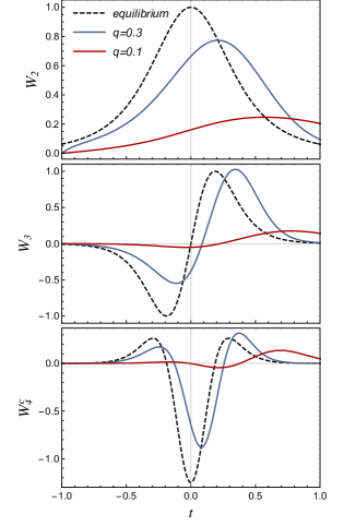
Figure 3: The time dependence of Wigner functions in comparison with their equilibrium value (dashed line) as the system is driven by expansion through the critical region. The evolution strongly depends on the scale of the fluctuations given by $q$ (see text).