Anomalies in gravitational charge algebras of null boundaries and black hole entropy

Abstract

Contents

1. 1 Introduction and summary
   1. 1.1 Notation
2. 2 Quasilocal charge algebra
   1. 2.1 Covariant phase space
   2. 2.2 Quasilocal charges
   3. 2.3 Barnich-Troessaert bracket
3. 3 Symplectic potential on a null boundary
   1. 3.1 Geometry of null hypersurfaces
   2. 3.2 Boundary conditions
   3. 3.3 Symplectic potential
   4. 3.4 Anomalous transformation of boundary term
   5. 3.5 Stretched horizon
4. 4 Virasoro symmetry
   1. 4.1 Near-horizon expansion
   2. 4.2 Expression for the noncovariance
   3. 4.3 Virasoro vector fields
   4. 4.4 Central charges
   5. 4.5 Frame dependence
5. 5 Entropy from the Cardy formula
   1. 5.1 Canonical Cardy formula
   2. 5.2 Integrable charges
   3. 5.3 Microcanonical Cardy formula
6. 6 Discussion
   1. 6.1 Algebra extension as a scaling anomaly
   2. 6.2 Barnich-Troessaert bracket and Dirichlet matching
   3. 6.3 Edge modes and the factor of 2
   4. 6.4 Future work
7. A Commutation relation for anomaly operator
8. B Derivation of the bracket identity
9. C Corner improvement
10. D Checking extension is central

1 Introduction and summary

Observables in general relativity tend to be global in nature, owing to the fact that diffeomorphisms are gauge symmetries of the theory. This large gauge redundancy causes the Hamiltonian of the theory to be localized to the asymptotic boundary, and diffeomorphism-invariant observables must be constructed relationally, using the fixed structures at the asymptotic boundary as points of reference [1, 2, 3]. Nonetheless, there exist notions of quasilocal observables that describe degrees of freedom inside of spatial subregions. In particular, several approaches to understanding the origin of black hole entropy deal with quasilocal charges on the event horizon [4, 5, 6, 7, 8, 9, 10, 11]. Moreover, charges associated with $\mathscr{I}$ in asymptotically flat space [12, 13, 14, 15, 16] and more general null surfaces [17, 18, 19, 20, 21, 22, 23] have received recent attention, due to their potential relevance to quantum gravity and flat space holography.

The appearance of quasilocal observables when considering subregions can be understood in terms of symmetry breaking. The introduction of a fixed boundary partially violates the diffeomorphism symmetry present in the theory, causing some transformations that were formerly considered gauge to become physical [4, 24]. The charges associated with the broken diffeomorphisms localize on the boundary of the subregion, and hence are referred to as edge modes [7, 25, 26]. The connection to black hole entropy comes from the proposal that the edge modes represent the degrees of freedom counted by the Bekenstein-Hawking entropy of a surface, given by $S_{\text{BH}}=\frac{A}{4G}$, with $A$ the area of the surface. The fact that the edge modes are localized on the boundary qualitatively explains the scaling with area, but in some examples the numerical coefficient can be computed in a precise manner. As first shown by Strominger for BTZ black holes in $\text{AdS}_{3}$ [27] using the Brown-Henneaux central charge [28], and subsequently generalized by Carlip to generic Killing horizons [4, 29], if the quasilocal charge algebra includes a Virasoro algebra, the entropy can be derived by applying the Cardy formula for the entropy of a 2D conformal field theory [30]. The rationale behind this procedure is that the Virasoro algebra is the symmetry algebra of 2D CFTs, so it is natural to conjecture that the quantization of the edge modes is given by a CFT, with the central charge determined by the classical brackets of the quasilocal charges. The precise agreement between the Cardy entropy and the Bekenstein-Hawking entropy then provides a posteriori justification for associating the entropy with edge mode degrees of freedom.

In most constructions in which the entropy arises from the Cardy formula applied to a boundary charge algebra, boundary conditions are needed to ensure the charges are integrable. The need for boundary conditions arises because the vector fields generating the symmetry have a transverse component to the codimension-2 surface on which the charge is being evaluated. This means they are generating a transformation that moves the bounding surface, and hence without boundary conditions, symplectic flux can leak out of the subregion as the system evolves. Imposing the boundary conditions ensures that the subregion behaves as a closed system, but gives the boundary the status of a physical barrier, preventing exchange of information between the subregion and its complement. When viewing the boundary as an arbitrary partition used to define a subregion, one would like a definition of quasilocal charges that does not employ such restrictive boundary conditions, and need not require conservation under time evolution. In the place of conservation, one seeks an independent definition of the flux of the quasilocal charge through the subregion boundary, so that the charge instead obeys a continuity equation. For general relativity and other diffeomorphism-invariant theories, Wald and Zoupas provided such a construction of quasilocal charges using covariant phase space techniques [12], and its application to null boundaries at a finite location was considered in [17].

Another reason for utilizing the Wald-Zoupas prescription is that in some cases, there is no obvious boundary condition that ensures integrability of the quasilocal charges. Such was the situation encountered by Haco, Hawking, Perry, and Strominger (HHPS) [10], who identified a set of near-horizon Virasoro symmetries for Kerr black holes, inspired by the hidden conformal symmetry of the near horizon wave equation identified in [31]. These symmetries suggest a possible extension of the results of the Kerr/CFT correspondence [32, 33], which deals with extremal Kerr black holes, to a holographic description of more general horizons. There does not exist a local boundary condition one can impose on the dynamical fields that is preserved by the HHPS vector fields, while simultaneously ensuring integrability of the corresponding charges. Hence, the Wald-Zoupas procedure is needed to define the quasilocal charges.

A specific form of the flux in the Wald-Zoupas prescription was conjectured in [10], and was also used in various subsequent works generalizing the construction [11, 35, 34, 36]. The goal of the present work is to derive the necessary Wald-Zoupas prescription for these constructions from first principles. In order to do so, there are three main technical challenges that need to be resolved.

First, there are a number of ambiguities that arise when carrying out the Wald-Zoupas construction, some of which affect the final result for the entropy. The most important ambiguity is in the ability to shift the symplectic potential on the bounding hypersurface by total variations, which subsequently affects the definitions of the charges and fluxes. To resolve this issue, we first reformulate the Wald-Zoupas procedure in section 2.2 using Harlow and Wu’s presentation of the covariant phase space formalism with boundaries [37]. Doing so allows for an efficient parameterization of the ambiguities that can appear in terms of boundary and corner terms in the variational principle. Rather than imposing boundary conditions to eliminate some terms that appear in the variations, as was done in [37], we interpret the nonzero boundary terms as representing a symplectic flux through the boundary. Explicitly, we decompose the pullback $\bm{\theta}$ of the symplectic potential current into boundary $\ell$, corner $\beta$, and flux $\mathcal{E}$ terms:

$$\bm{\theta}+\delta\ell=d\beta+\mathcal{E}.$$ (1.1)

Resolving the ambiguities in the Wald-Zoupas prescription then amounts to finding a preferred choice for the flux term $\mathcal{E}$.

We propose a principle for fixing this ambiguity in section 2.2, namely that $\mathcal{E}$ should be of Dirichlet form, meaning it involves variations only of intrinsic quantities on the surface. It therefore is expressible as

$$\mathcal{E}=\pi^{ij}\delta g_{ij},$$ (1.2)

where $\delta g_{ij}$ is the variation of the induced metric on the bounding hypersurface, and $\pi^{ij}$ are the conjugate momenta constructed from extrinsic quantities. For null hypersurfaces, the variation of the null generator $\delta l^{i}$ is also considered an intrinsic quantity, so the Dirichlet form of the flux in this case reads

$$\mathcal{E}=\pi^{ij}\delta g_{ij}+\pi_{i}\delta l^{i}.$$ (1.3)

The terminology “Dirichlet” refers to the fact that vanishing flux is equivalent to Dirichlet boundary conditions for this choice. The Dirichlet flux condition is a novel proposal in the context of the Wald-Zoupas construction, in contrast with previous proposals which employed properties of the flux in stationary solutions to partially fix its form [38, 17]. However, it is familiar from the Brown-York procedure for quasilocal energy [39], and has a natural interpretation in the context of holography. We also argue that this form of the flux is preferred from the perspective of gluing subregions together in the gravitational path integral [40]. As a byproduct of fixing this form of the flux, we can also employ Harlow and Wu’s [37] resolution of the standard Jacobson-Kang-Myers ambiguities in the covariant phase space formalism [41, 42], leading to unambiguous definitions of the quasilocal charges.

The second issue to address is the problem of constructing a bracket for the quasilocal charges that defines their algebra. Poisson brackets are not available when employing the Wald-Zoupas procedure, since we are dealing with an open system with respect to the symplectic flux. Therefore, in section 2.3, we instead utilize the bracket defined by Barnich and Troessaert in [43] for nonintegrable charges. It has the advantage of representing the algebra satisfied by the vector fields generating the symmetry transformations, up to abelian extensions. We further show that the algebra extension has a simple expression

$$K_{\xi,\zeta}=\int_{\partial\Sigma}\Big{(}i_{\xi}\Delta_{\hat{\zeta}}\ell-i_{\zeta}\Delta_{\hat{\xi}}\ell\Big{)}$$ (1.4)

in terms of $\Delta_{\hat{\xi}}\ell$, the anomalous transformation with respect to the symmetry generator $\xi^{a}$ of the boundary term $\ell$ in (1.1). The anomaly operator $\Delta_{\hat{\xi}}$, defined in (2.1), directly measures the failure of an object to transform covariantly under the diffeomorphism generated by $\xi^{a}$, and hence we immediately see that algebra extensions only appear when the boundary term $\ell$ is not covariant with respect to the transformation. Because the Barnich-Troessaert bracket coincides with the Poisson bracket when the charges are integrable, this formula for the extension applies in the case of integrable charges as well. This shows quite generally that central charges and abelian extensions appear as a type of classical anomaly associated with the boundary term in the variational principle. This statement is directly analogous to the appearance of holographic Weyl anomalies in AdS/CFT [44, 45, 46, 47].

The third issue to address is finding a decomposition of the symplectic potential for general relativity when restricted to a null boundary $\mathcal{N}$. This question has been treated in previous analyses [17, 48, 18, 19, 49, 50]; however, most of these employ boundary conditions that are too strong to allow for the symmetries generated by the HHPS vector fields. In our analysis in section 3, we employ the weakest possible boundary conditions that ensure the presence of a null surface, and in which the variations of all quantities are entirely determined in terms of $\delta g_{ab}$. This is done by fixing the normal covector, $\delta l_{a}=0$, and imposing nullness by requiring that $l^{a}l^{b}\delta g_{ab}=0$ on $\mathcal{N}$. The covector $l_{a}$ is thus viewed as a background structure introduced into the theory in order to define the boundary. Because it is a background structure, no issues arise if the symmetry generators do not preserve it; in fact, the failure of $l_{a}$ to be preserved by the symmetry generators is the sole source of noncovariance in the construction, and hence is responsible for the appearance of a nonzero central charge. By contrast, it is crucial that the vector fields satisfy $l^{a}l^{b}\pounds_{\xi}g_{ab}=0$ on $\mathcal{N}$, since this arises from a boundary condition imposed on the dynamical metric; violating it would cause the symmetry transformations to be ill-defined. The HHPS vector fields satisfy this condition, as do any vectors which preserve the null surface.

The result of the decomposition of the symplectic potential is given in equations (3.26)–(3.30), in which the Dirichlet form of $\mathcal{E}$ is decomposed into $\frac{d(d-1)}{2}$ canonical pairs on the null surface. The decomposition that we find has appeared before in [48], and related decompositions can be found in [18, 19]. The boundary term $\ell$ that arises in the decomposition is constructed from the inaffinity $k$ of the null generator $l^{a}$, and has appeared in previous analyses on null boundary terms in the action for general relativity [48, 18, 50]. In particular, we find additional flux terms beyond those employed in [10, 34], whose presence is necessary to ensure that the flux is independent of the choice of auxiliary null vector $n_{a}$.

With all this in place, we give a systematic analysis in section 4 of the quasilocal charges in the HHPS construction, as well as the generalization to arbitrary bifurcate, axisymetric Killing horizons [10, 34]. The symmetry algebra consists of two copies of the Virasoro algebra, and the central charges are computed to be

$$c=\bar{c}=\frac{3A}{\pi G(\alpha+\bar{\alpha})},$$ (1.5)

where $\alpha$ and $\bar{\alpha}$ are two parameters characterizing the symmetry generators, and are related to the choice of left and right temperatures. These values of $c$, $\bar{c}$ are twice the value given in [10, 34], and consequently, when applying the Cardy formula in section 5.1, we find that the entropy is twice the Bekenstein-Hawking entropy of the horizon. We take this as an indication that the quasilocal charge algebra is sensitive to degrees of freedom associated with the complementary region. In particular, we note that the factor of $2$ could be explained if the central charge appearing in the Barnich-Troessaert bracket was associated with a pair of quasilocal charge algebras, one on each side of the dividing surface. This interpretation is further motivated by the conjectured edge mode contribution to entanglement entropy in gravitational theories, which employ such a pair of quasilocal charges at an entangling surface [7]. The doubling of $c$, $\bar{c}$ would then be intimately related to the fact that we are considering an open system that is interacting with its complement. Conversely, if the charges were instead integrable so that they lived in a closed system, we would expect the standard entropy to arise via the Cardy formula. We demonstrate that this is the case in sections 5.2 and 5.3 by showing that a different boundary term is needed in order to find integrable generators. The new boundary term halves the value of the central charges and the entropy, and also leads to agreement between the microcanonical and canonical Cardy formulas.

In section 6, we further discuss the interpretation of these results, and describe some directions for future work.

Note added:

This work is being released in coordination with [51], which explores some related topics.

1.1 Notation

We work in arbitrary spacetime dimension $d$ with metric signature $(-,+,+,\ldots)$. Spacetime tensors will be written with abstract indices $a,b,\ldots$, such as the metric $g_{ab}$. We denote null hypersurfaces by $\mathcal{N}$, and indices $i,j,\ldots$ will denote tensors defined on $\mathcal{N}$, such as $q_{ij}$ and $l^{k}$. An equality that only holds at the location of $\mathcal{N}$ in spacetime will be written as $\mathrel{\mathop{\widehat{=}}}$. Differential forms will often be written without indices, and, when necessary, we distinguish a form $\theta$ defined on spacetime from its pullback ${\bm{\theta}}$ to $\mathcal{N}$ using boldface. The null normal to $\mathcal{N}$ will be denoted $l_{a}$, and the auxiliary null vector will be denoted $n^{a}$. The volume form on spacetime is denoted $\epsilon$, and occasionally it will be written as $\epsilon_{a}$ or $\epsilon_{ab}$ when the displayed indices are being contracted; the undisplayed indices are left implicit. The volume form on $\mathcal{N}$ induced from $l_{a}$ will be denoted $\eta$, and the horizontal spatial volume form on $\mathcal{N}$ will be denoted $\mu$. The notation for the contraction of a vector $v^{a}$ into a differential form $m$ is $i_{v}m$. The notation for operations defined on $\mathcal{S}$, the space of solutions to the field equations, is described in section 2.1 below, including definitions of $I_{\hat{\xi}}$, $L_{\hat{\xi}}$, $\delta$, and $\Delta_{\hat{\xi}}$.

2 Quasilocal charge algebra

We begin by reviewing the covariant phase space construction in section 2.1, before turning to the construction of quasilocal charges in section 2.2, and their algebra in section 2.3. Section 2.2 explains the relation between the Wald-Zoupas construction [12] and the recent work by Harlow and Wu on the covariant phase space with boundaries [37]. This yields an unambiguous definition of the quasilocal charges by the arguments of [37], once the form of the flux $\mathcal{E}$ has been specified. To fix this final ambiguity, we require that the flux be of Dirichlet form, and we discuss the motivation for this choice coming from the combined variational principle for the subregion and its complement. The algebra of charges is then defined in section 2.3, where we give a general expression for the extension of the algebra in terms of the anomaly of the boundary term appearing in the symplectic potential decomposition.

2.1 Covariant phase space

The main tool we employ in constructing the quasilocal charge algebra is the covariant phase space [52, 53, 54, 55, 56]. It provides a canonical description of field theories without singling out a preferred time foliation, and therefore is well-suited for handling diffeomorphism-invariant theories, such as general relativity. Covariance is achieved by working with the space $\mathcal{S}$ of solutions to the field equations, as opposed to the space of initial data on a time slice.

$\mathcal{S}$ can be viewed as an infinite-dimensional manifold, on which many standard differential-geometric techniques apply. Fields such as the metric $g_{ab}$ can be viewed as functions on $\mathcal{S}$, and their variations, such as $\delta g_{ab}$, are one-forms. The operation $\delta$ of taking variations can be viewed as the exterior derivative on $\mathcal{S}$, and forms of higher degree can be built by taking exterior derivatives and wedge products in the usual way. The product of two differential forms $\alpha$ and $\beta$ on $\mathcal{S}$ will always implicitly be a wedge product, so that $\alpha\beta=(-1)^{\deg(\alpha)\deg(\beta)}\beta\alpha$, which allows the symbol $\wedge$ to exclusively denote the wedge product between differential forms on the spacetime manifold $\mathcal{M}$. We denote by $I_{V}$ the operation of contracting a vector field $V$ on $\mathcal{S}$ with a differential form. Functions of the form $h_{ab}=I_{V}\delta g_{ab}$ are simply solutions to the linearized field equations, and so the vector fields on $\mathcal{S}$ are seen to coincide with the space of linearized solutions.

Since diffeomorphisms of $\mathcal{M}$ are gauge symmetries of general relativity, they define an important subclass of linearized solutions $h_{ab}=\pounds_{\xi}g_{ab}$, where $\xi^{a}$ is a spacetime vector field. The corresponding vector field on $\mathcal{S}$ generating this transformation will be called $\hat{\xi}$, which satisfies $I_{\hat{\xi}}\delta g_{ab}=\pounds_{\xi}g_{ab}$. Note also that $I_{\hat{\xi}}\delta g_{ab}=L_{\hat{\xi}}g_{ab}$, where $L_{\hat{\xi}}$ is the Lie derivative along the vector $\hat{\xi}$ in $\mathcal{S}$, and hence $L_{\hat{\xi}}$ and $\pounds_{\xi}$ agree when acting on the metric $g_{ab}$. The action of $L_{\hat{\xi}}$ on higher order differential forms on $\mathcal{S}$ can be computed via the Cartan formula $L_{\hat{\xi}}=I_{\hat{\xi}}\delta+\delta I_{\hat{\xi}}$. Any differential form $\alpha$ that is locally constructed from dynamical fields and for which $L_{\hat{\xi}}\alpha=\pounds_{\xi}\alpha$ will be called covariant with respect to $\hat{\xi}$. Since we later work with noncovariant objects as well, it is useful to define the anomaly operator

$$\Delta_{\hat{\xi}}=L_{\hat{\xi}}-\pounds_{\xi},$$ (2.1)

as in [19], which measures the failure of a local object to be covariant. We therefore also refer to $\Delta_{\hat{\xi}}\alpha$ as the noncovariance or anomaly of $\alpha$ with respect to $\hat{\xi}$. As we will see, $\Delta_{\hat{\xi}}$ plays a prominent role in characterizing the extensions that appear in quasilocal charge algebras, and the anomalies it computes are, in many ways, classical analogs of the anomalies that appear in quantum field theories. In particular, as we show in appendix A, $\Delta_{\hat{\xi}}$ satisfies

$$[\Delta_{\hat{\xi}},\Delta_{\hat{\zeta}}]=-\Delta_{\widehat{[\xi,\zeta]}},$$ (2.2)

which, when imposed on the functionals of the theory, is the direct analog of the Wess-Zumino consistency condition for quantum anomalies [57].

The covariant phase space arises from $\mathcal{S}$ by imbuing it with a presymplectic form. To construct it, one begins with the Lagrangian of the theory, $L$, which is a spacetime top form whose variation satisfies

$$\delta L=E^{ab}\delta g_{ab}+d\theta,$$ (2.3)

where $E^{ab}=0$ are the classical field equations, and $\theta$ is a one-form on $\mathcal{S}$ and a $(d-1)$-form on spacetime called the symplectic potential current. For general relativity, the various quantities are

$$L =\frac{1}{16\pi G}(R-2\Lambda)\epsilon$$ (2.4)

$$E^{ab} =\frac{-\epsilon}{16\pi G}\left(R^{ab}-\frac{1}{2}Rg^{ab}+\Lambda g^{ab}\right)$$ (2.5)

$$\theta =\frac{1}{16\pi G}\epsilon_{a}\Big{(}g^{bc}\delta\Gamma^{a}_{bc}-g^{ac}\delta\Gamma^{b}_{bc}\Big{)},$$ (2.6)

where the variation of the Christoffel symbol is

$$\delta\Gamma^{a}_{bc}=\frac{1}{2}g^{ad}\left(\nabla_{b}\delta g_{dc}+\nabla_{c}\delta g_{bc}-\nabla_{d}\delta g_{bc}\right),$$ (2.7)

and we recall that $\epsilon_{a}$ still denotes the spacetime volume form, with uncontracted indices not displayed.

The $\mathcal{S}$-exterior derivative of $\theta$ defines the symplectic current $\omega=\delta\theta$, and its integral over a Cauchy surface $\Sigma$ for the region of spacetime under consideration yields the presymplectic form,

$$\Omega=\int_{\Sigma}\omega.$$ (2.8)

$\Omega$ is called “presymplectic” because it contains degenerate directions corresponding to diffeomorphisms of $\mathcal{M}$. Since diffeomorphisms are symmetries of the Lagrangian, they lead to Noether currents that are conserved on shell, given by

$$J_{\xi}=I_{\hat{\xi}}\theta-i_{\xi}L.$$ (2.9)

Because $dJ_{\xi}=0$ identically for all vectors $\xi^{a}$, the Noether current can be written as the exterior derivative of a potential, $J_{\xi}=dQ_{\xi}$, which is locally constructed from the metric; for general relativity, this potential is [59, 38],

$$Q_{\xi}=\frac{-1}{16\pi G}\epsilon\indices{{}^{a}_{b}}\nabla\indices{{}_{a}}\xi^{b}.$$ (2.10)

The degeneracy of $\Omega$ follows straightforwardly from computing the contraction with $I_{\hat{\xi}}$,

$$-I_{\hat{\xi}}\Omega=\int_{\partial\Sigma}\Big{(}\delta Q_{\xi}-i_{\xi}\theta\Big{)},$$ (2.11)

using the fact that $\theta$ is covariant, $I_{\hat{\xi}}\delta\theta+\delta I_{\hat{\xi}}\theta=\pounds_{\xi}\theta$ [42]. Since this contraction localizes to a boundary integral, any diffeomorphism that acts purely in the interior is a degenerate direction of $\Omega$. The phase space $\mathcal{P}$ is a quotient of $\mathcal{S}$ by the degenerate directions, onto which $\Omega$ descends to a nondegenerate symplectic form [56].

2.2 Quasilocal charges

According to (2.11), diffeomorphisms with support near the Cauchy surface boundary $\partial\Sigma$ are not degenerate directions; rather, they lead to a notion of quasilocal charges associated with the subregion defined by $\Sigma$. In the case that $\xi^{a}$ at $\partial\Sigma$ is vanishing or tangential, the term $i_{\xi}\theta$ in (2.11) drops out when pulled back to $\partial\Sigma$, and a Hamiltonian for the transformation can be defined by

$$H_{\xi}=\int_{\partial\Sigma}Q_{\xi},$$ (2.12)

which generates the symmetry transformation on phase space via Hamilton’s equations,

$$\delta H_{\xi}=-I_{\hat{\xi}}\Omega.$$ (2.13)

When $\xi^{a}$ is not tangential to $\partial\Sigma$, $-I_{\hat{\xi}}\Omega$ generally cannot be written as a total variation, unless boundary conditions are imposed so that $\int_{\partial\Sigma}i_{\xi}\theta=\delta B_{\xi}$ for some quantity $B_{\xi}$. Such boundary conditions are natural when $\partial\Sigma$ sits at an asymptotic boundary, but not at boundaries associated with subregions of a larger system, where the boundary conditions are generically inconsistent with the global dynamics. Instead, one can define a quasilocal charge associated with the transformation following the Wald-Zoupas prescription [12]. The quasilocal charge is not conserved since it fails to satisfy Hamilton’s equation (2.13), but it satisfies a modified equation that relates the nonconservation to a well-defined flux through the boundary of the subregion.

Figure 1: In the Wald-Zoupas construction, one seeks to construct quasilocal charges for a transformation generated by $\xi^{a}$, which is tangent to a hypersurface $\mathcal{N}$ bounding an open subregion $\mathcal{U}$ to the right of $\mathcal{N}$. The charges are constructed as integrals over a codimension-2 surface $\partial\Sigma$, bounding a Cauchy surface $\Sigma$ for the subregion. The vector field $\xi^{a}$ can have both tangential and normal components to $\partial\Sigma$. In this figure, $\mathcal{N}$ is a null hypersurface, and the Cauchy surface has been chosen to include a segment of $\mathcal{N}$.

Here, we give a presentation of the Wald-Zoupas construction, using the formalism developed by Harlow and Wu [37] for dealing with boundaries in the covariant phase space. The Wald-Zoupas construction begins with a subregion of spacetime $\mathcal{U}$, bounded by a hypersurface $\mathcal{N}=\partial\mathcal{U}$ (see figure 1). Later $\mathcal{N}$ will be taken to be a null hypersurface, but the present discussion applies more generally for any signature of $\mathcal{N}$. On $\mathcal{N}$, one looks for a decomposition of the pullback ${\bm{\theta}}$ of the symplectic potential of the following form

$${\bm{\theta}}=-\delta\ell+d\beta+\mathcal{E}$$ (2.14)

where $\ell$ is referred to as the boundary term, $\beta$ is the corner term, and $\mathcal{E}$ is the flux term. The reason for this terminology becomes apparent from the variational principle for the theory defined in the subregion $\mathcal{U}$ [37, 61]. The action for the subregion is

$$S=\int_{\mathcal{U}}L+\int_{\mathcal{N}}\ell,$$ (2.15)

and by the decomposition (2.14) the variation satisfies

$$\delta S=\int_{\mathcal{U}}E^{ab}\delta g_{ab}+\int_{\mathcal{N}}\left(\mathcal{E}+d\beta\right),$$ (2.16)

and so the action is stationary when the bulk field equations $E^{ab}=0$ hold and boundary conditions are chosen to make $\mathcal{E}$ vanish, with the $d\beta$ term localizing to the boundary of $\mathcal{N}$, i.e. the corner. In the Wald-Zoupas setup, boundary conditions to make $\mathcal{E}$ vanish are not imposed; instead, $\mathcal{E}$ is used to construct the fluxes of the quasilocal charges. In [12], the combination $\mathcal{E}+d\beta$ is referred to as a potential for the pullback of $\omega$ to $\mathcal{N}$, since by equation (2.14) we see that

$$\delta(\mathcal{E}+d\beta)=\delta{\bm{\theta}}={\bm{\omega}}.$$ (2.17)

The corner term $\beta$ is used to modify the symplectic form for the subregion. This is done by extending $d\beta$ to an exact form on all of $\mathcal{U}$, and then treating $\theta-d\beta$ as the symplectic potential current. The symplectic form then becomes

$$\Omega=\int_{\Sigma}\omega-\int_{\partial\Sigma}\delta\beta.$$ (2.18)

We can then evaluate the contraction of $\Omega$ with a diffeomorphism generator $\xi^{a}$ that is parallel to $\mathcal{N}$, but not necessarily to $\partial\Sigma$,

$$-I_{\hat{\xi}}\Omega =\int_{\partial\Sigma}\Big{(}\delta Q_{\xi}-i_{\xi}\theta+I_{\hat{\xi}}\delta\beta\Big{)}$$

$$=\int_{\partial\Sigma}\Big{(}\delta Q_{\xi}+i_{\xi}\delta\ell-\delta I_{\hat{\xi}}\beta\Big{)}-\int_{\partial\Sigma}\Big{(}i_{\xi}\mathcal{E}-\Delta_{\hat{\xi}}\beta\Big{)}.$$ (2.19)

The first term is the total variation of a quantity

$$H_{\xi}=\int_{\partial\Sigma}\Big{(}Q_{\xi}+i_{\xi}\ell-I_{\hat{\xi}}\beta\Big{)},$$ (2.20)

which we call the quasilocal charge for the transformation. The second term in (2.19) represents the failure of the quasilocal charge to be an integrable generator of the symmetry. Assuming that $\beta$ is covariant, so that $\Delta_{\hat{\xi}}\beta=0$, the obstruction to integrability of the charge is simply given by the integral of the flux density $i_{\xi}\mathcal{E}$. With slight modifications, the case where $\Delta_{\hat{\xi}}\beta\neq 0$ can be handled, and is described in appendix C. Equation (2.19) can be rearranged slightly to take the form of a modified Hamilton’s equation,

$$\delta H_{\xi}=-I_{\hat{\xi}}\Omega+\int_{\partial\Sigma}i_{\xi}\mathcal{E}$$ (2.21)

To further the interpretation of $\mathcal{E}$ as a flux of $H_{\xi}$, we note first that the integrand of (2.20) is defined on all of $\mathcal{N}$, and its exterior derivative can be computed as

$$d\left(Q_{\xi}+i_{\xi}\ell-I_{\hat{\xi}}\beta\right) =I_{\hat{\xi}}{\bm{\theta}}-i_{\xi}L-i_{\xi}d\ell+\pounds_{\xi}\ell-I_{\hat{\xi}}d\beta$$

$$=I_{\hat{\xi}}\mathcal{E}-\Delta_{\hat{\xi}}\ell-i_{\xi}(L+d\ell)$$ (2.22)

Integrating this relation on a segment $\mathcal{N}_{1}^{2}$ of $\mathcal{N}$ between two cuts $S_{2}$ and $S_{1}$, and using that $\xi^{a}$ is parallel to $\mathcal{N}$ yields

$$H_{\xi}(S_{2})-H_{\xi}(S_{1})=\int_{\mathcal{N}_{1}^{2}}\Big{(}I_{\hat{\xi}}\mathcal{E}-\Delta_{\hat{\xi}}\ell\Big{)}.$$ (2.23)

This can be interpreted as an anomalous continuity equation for the quasilocal charge $H_{\xi}$: the difference in the charge between two cuts is simply given by the flux $F_{\xi}=\int_{\mathcal{N}_{1}^{2}}I_{\hat{\xi}}\mathcal{E}$, up to an anomalous contribution from $\Delta_{\hat{\xi}}\ell$. This anomalous term in the flux vanishes if $\ell$ is covariant with respect to $\xi^{a}$; however, we will find that on null surfaces, the most natural choice for the flux term $\mathcal{E}$ requires a boundary term that is not covariant. Note that this equation differs from the standard continuity equation derived in the Wald-Zoupas and related constructions [17, 12, 60, 21], which assume a covariant boundary term, so that $\Delta_{\hat{\xi}}\ell$ drops out. This is the first indication that the noncovariance of the boundary term can be interpreted as an anomaly, since it behaves as an explicit violation of a contintuity equation for the quasilocal charges. In quantum field theory, anomalies play a similar role to that of $\Delta_{\hat{\xi}}\ell$, where they lead to explicit violations of the Ward identities.

Up to this point, we have placed no restrictions on the precise form of the flux $\mathcal{E}$. Equation (2.14) does not uniquely specify $\mathcal{E}$, since it can always be shifted by terms of the form $\mathcal{E}\rightarrow\mathcal{E}-\delta b-d\lambda$ by making compensating changes $\ell\rightarrow\ell-b$, $\beta\rightarrow\beta+\lambda$. These ambiguities in $\mathcal{E}$ are similar in appearance to the standard Jacobson-Kang-Myers ambiguities [41, 42] in the definition of the symplectic potential current, in which $\theta\rightarrow\theta+\delta b^{\prime}+d\lambda^{\prime}$. Although the $(b,\lambda)$ and $(b^{\prime},\lambda^{\prime})$ ambiguities are in principle distinct, they can be used in tandem to leave $\mathcal{E}$ invariant, by setting $(b,\lambda)=(b^{\prime},\lambda^{\prime})$. Additionally, the charge densities $h_{\xi}=Q_{\xi}+i_{\xi}\ell-I_{\hat{\xi}}\beta$ are also unchanged, provided one shifts the Noether potential by $Q_{\xi}+i_{\xi}b^{\prime}+I_{\hat{\xi}}\lambda^{\prime}$, as was recently emphasized by [37]. These transformations of $Q_{\xi}$ simply follow from its definition as a potential for the Noether current $J_{\xi}$ (2.9) as long as one assumes that $b^{\prime}$ is covariant (no assumption on the covariance properties of $\gamma^{\prime}$ is needed).

Thus, in order to avoid the ambiguities just described, we need to fix the form of the flux $\mathcal{E}$. As discussed in [61, 64], different choices for $\mathcal{E}$ are related to different boundary conditions one would impose to make the flux vanish. The principle we will advocate for in this work is that the flux take a Dirichlet form, which, for $\mathcal{N}$ timelike or spacelike, means it is written as

$$\mathcal{E}=\pi^{ij}\delta g_{ij},$$ (2.24)

where $\delta g_{ij}$ is the metric variation pulled back to $\mathcal{N}$, constituting the intrinsic data on the surface, and $\pi^{ij}$ is a symmetric-tensor-valued top form on $\mathcal{N}$ constructed from the extrinsic data, and interpreted as the conjugate momenta to $\delta g_{ij}$. The intrinsic data on a null surface is slightly different since the induced metric is degenerate, and so it is taken to also include variations of the null generator $\delta l^{i}$, leading to the null Dirichlet flux condition

$$\mathcal{E}=\pi^{ij}\delta g_{ij}+\pi_{i}\delta l^{i}.$$ (2.25)

Dependence on non-intrinsic components of the metric, such as the lapse and shift, is removed by the choice of corner term, which further fixes the ambiguities in specifying the flux. Imposing the Dirichlet form on $\mathcal{E}$ greatly reduces the freedom in its definition, since most of the ambiguities will involve variations of quantities constructed from the extrinsic geometry of $\mathcal{N}$. We will find that for general relativity, the Dirichlet requirement fixes $\mathcal{E}$ essentially uniquely.

One reason for favoring the Dirichlet form of the flux comes from considering the variational principle for a subregion $\mathcal{U}$ and its complement $\bar{\mathcal{U}}$. When gluing the subregions across the boundaries $\mathcal{N}$ and $\bar{\mathcal{N}}$, the Dirichlet form of $\mathcal{E}$ is used when kinematically matching the intrinsic quantities on $\mathcal{N}$. Viewed from one side, this takes the form of a Dirichlet condition, with the value of $g_{ij}$ on one side fixed by the value on the other side. Upon identifying $\mathcal{N}$ with $\bar{\mathcal{N}}$, matching $g_{ij}$, and imposing the bulk field equations, the variation of the action is given by

$$\delta\left(\int_{\mathcal{U}}L+\int_{\mathcal{N}}\ell+\int_{\bar{\mathcal{N}}}\bar{\ell}+\int_{\bar{\mathcal{U}}}L\right)=\int_{\mathcal{N}}(\pi^{ij}-\bar{\pi}^{ij})\delta g_{ij}+\text{corner term}.$$ (2.26)

Stationarity of the action then dynamically sets $\pi^{ij}-\bar{\pi}^{ij}=0$, or more generally equal to the distributional stress energy on $\mathcal{N}$ if present, according to the junction conditions [69, 70]. If instead a Neumann form for the flux $\mathcal{E}^{N}=-g_{ij}\delta\pi^{ij}$ were employed, the matching condition would kinematically set $\pi^{ij}=\bar{\pi}^{ij}$, and then $g_{ij}-\bar{g}_{ij}$ would dynamically be set to zero. In this case, there does not appear to be a straightforward way to allow for distributional stress-energy on $\mathcal{N}$. In vacuum, the end result is classically the same, with both $g_{ij}$ and $\pi^{ij}$ matching at $\mathcal{N}$, although already the Dirichlet form has the advantage of allowing for the presence of distributional stress-energy. In a quantum description, these two options differ even more. Since the path integral receives contributions from off-shell configurations, the Dirichlet matching appears to be preferred, since the Neumann matching allows for discontinuities in the intrinsic metric, which produce distributionally ill-defined curvatures [70]. We further discuss the Dirichlet matching condition in section 6.2.

2.3 Barnich-Troessaert bracket

Having defined the quasilocal charges $H_{\xi}$ given by (2.20) for the diffeomorphisms generated by $\xi^{a}$, we now consider the problem of computing their algebra. In standard Hamiltonian mechanics, this is given by the Poisson bracket constructed from the symplectic form of the system. When the charges are integrable, so that they satisfy Hamilton’s equation (2.13), the Poisson bracket can be evaluated by contracting the vector fields generating the symmetry into the symplectic form,

$$\{H_{\xi},H_{\zeta}\}=-I_{\hat{\xi}}I_{\hat{\zeta}}\Omega=-\left(H_{[\xi,\zeta]}+K_{\xi,\zeta}\right).$$ (2.27)

The second equality in this equation is a statement of the fact that Poisson brackets must reproduce the Lie bracket of the vector fields $\xi^{a}$, $\zeta^{a}$, up to a central extension, denoted $K_{\xi,\zeta}$.

For quasilocal charges, their failure to satisfy Hamilton’s equations due to the flux term in (2.21) prevents a naive application of (2.27) to their brackets. Instead, Barnich and Troessaert [43] proposed a modification to the bracket that accounts for the nonconservation of the charges due to the loss of flux from the subregion. When the corner term $\beta$ is covariant, their bracket is given by

$$\{H_{\xi},H_{\zeta}\}=-I_{\hat{\xi}}I_{\hat{\zeta}}\Omega+\int_{\partial\Sigma}\Big{(}i_{\zeta}I_{\hat{\xi}}\mathcal{E}-i_{\xi}I_{\hat{\zeta}}\mathcal{E}\Big{)},$$ (2.28)

where we see that the bracket is modified by the fluxes $F_{\xi}=\int_{\partial\Sigma}I_{\hat{\xi}}\mathcal{E}$ identified in the Wald-Zoupas construction. A heuristic way to understand this equation is as follows: imagine adding an auxiliary system which collects the flux lost through $\mathcal{N}$ when evolving along $\xi^{a}$ (for example, this could just be the phase space associated with the complementary region $\bar{\mathcal{U}}$). The total system consisting of the subregion and the auxiliary system is assumed to have a Poisson bracket defined on it, such that $\hat{\xi}$ is a symmetry of the bracket in the usual sense. The Hamiltonian for $\hat{\xi}$ should be a sum of the quasilocal Hamiltonian $H_{\xi}$ and a term $H_{\xi}^{\text{aux}}$ associated with the auxiliary system. Hamilton’s equation for the total system then reads

$$I_{\hat{\xi}}\delta H_{\zeta}=\{H_{\xi}+H_{\xi}^{\text{aux}},H_{\zeta}\}.$$ (2.29)

The contribution from $\{H_{\xi}^{\text{aux}},H_{\zeta}\}$ should compute the flux of $H_{\zeta}$ into the auxiliary system due to an infinitesimal change of $\partial\Sigma$ along $\xi^{a}$, which is just the integral of $i_{\xi}I_{\hat{\zeta}}\mathcal{E}$, given our identification of $I_{\hat{\zeta}}\mathcal{E}$ with the flux density. Equation (2.29) then becomes

$$I_{\hat{\xi}}\delta H_{\zeta}=\{H_{\xi},H_{\zeta}\}+\int_{\partial\Sigma}i_{\xi}I_{\hat{\zeta}}\mathcal{E},$$ (2.30)

which reduces to (2.28) after using the expression (2.21) for $\delta H_{\zeta}$. Going forward, we will take (2.28) as the definition of the bracket for the quasilocal charges, and delay further discussion of its interpretation to section 6.2.

An important property of the Barnich-Troessaert bracket is that it reproduces the Lie bracket algebra of the vector fields, up to abelian extensions [43, 72]. This can be explicitly verified using the expression (2.20) for the quasilocal charges, and an exact expression for the extension $K_{\xi,\zeta}$ can be given. After a short calculation (see appendix B), one finds

$$\{H_{\xi},H_{\zeta}\} =-\left(H_{[\xi,\zeta]}+K_{\xi,\zeta}\right)$$ (2.31)

$$K_{\xi,\zeta} =\int_{\partial\Sigma}\Big{(}i_{\xi}\Delta_{\hat{\zeta}}\ell-i_{\zeta}\Delta_{\hat{\xi}}\ell\Big{)}.$$ (2.32)

Hence, we arrive at one of the main results of this work, namely, that the extension $K_{\xi,\zeta}$ is determined entirely by the noncovariance of the boundary term, $\Delta_{\hat{\xi}}\ell$. As an immediate corollary, we see that the extension $K_{\xi,\zeta}$ always vanishes if the boundary term $\ell$ is covariant with respect to the generators $\xi^{a}$. Equation (2.32) remains valid even when boundary conditions are imposed to ensure the transformation has integrable generators. In this case, the fluxes in (2.28) vanish, and we see that the Barnich-Troessaert bracket reduces to a Dirac bracket on the subspace of field configurations that satisfy the boundary conditions. This therefore gives a universal formula for the central extension in these cases, in addition to the more general cases involving nonintegrable generators.

It is worth emphasizing that the central charge appears in this formula because we have chosen to fix a background structure in defining the boundary, which gives rise to nonzero anomalies $\Delta_{\hat{\xi}}\ell$. However, the value of $K_{\xi,\zeta}$ does not depend on the choice of constant added to the Hamiltonians, which, for example, could be chosen to ensure that the Hamiltonians vanish in a given background solution. More precisely, different choices for these constant shifts can only change the extension by trivial constant terms of the form $C_{[\xi,\zeta]}$, which will not change the 2-cocycle that $K_{\xi,\zeta}$ represents for the Lie algebra of the vector fields $\xi^{a},\zeta^{a}$. In particular, $C_{[\xi,\zeta]}$ cannot be chosen to cancel $K_{\xi,\zeta}$ if the extension comes from a nontrivial 2-cocycle, as occurs in the Virasoro example we consider in section 4.

In general, the new generators $K_{\xi,\zeta}$ are not central, since they are allowed to transform nontrivially under the action of another generator $H_{\chi}$. Instead, they give an abelian extension of the algebra by defining their brackets to be

$$\{H_{\chi},K_{\xi,\zeta}\} =I_{\hat{\chi}}\delta K_{\xi,\zeta}$$ (2.33)

$$\{K_{\xi,\zeta},K_{\chi,\psi}\} =0.$$ (2.34)

This algebra closes provided $I_{\hat{\chi}}\delta K_{\xi,\zeta}$ is expressible as a sum of other generators $K_{\xi^{\prime},\zeta^{\prime}}$, and the Jacobi identity holds as long as $K_{\xi,\zeta}$ satisfies a generalized cocycle condition [43],

$$I_{\hat{\chi}}\delta K_{\xi,\zeta}+K_{[\chi,\xi],\zeta}+(\text{cyclic $\chi\rightarrow\xi\rightarrow\zeta$})=0.$$ (2.35)

Of course, when the right hand side of (2.33) vanishes, $K_{\xi,\zeta}$ represents a central extension of the algebra.

We verify the above cocycle condition for (2.32) in appendix B. We should expect this to be the case because $K_{\xi,\zeta}$ in (2.32) is of the form of a trivial field-dependent 2-cocycle, in the terminology of [43]. That is, it can be expressed as

$$K_{\xi,\zeta}=I_{\hat{\zeta}}\delta B_{\xi}-I_{\hat{\xi}}\delta B_{\zeta}-B_{[\xi,\zeta]},\qquad B_{\xi}\equiv\int_{\partial\Sigma}i_{\xi}\ell$$ (2.36)

Despite this terminology, $K_{\xi,\zeta}$ is certainly not required to be trivial as a cocycle for the Lie algebra generated by the vector fields. This will be explicitly demonstrated for the algebra considered in section 4, in which case $K_{\xi,\zeta}$ becomes the nontrivial central extension of the Witt algebra to Virasoro.

Finally, it is worth noting that the corner term $\beta$, although important in arriving at the Dirichlet form (2.24) or (2.25) for the flux, is not important for obtaining the correct algebra for the quasilocal charges, including the extension $K_{\xi,\zeta}$. Algebraically, the $\beta$ term in the quasilocal charge is functioning as a trivial extension of the algebra, since the $\beta$ terms do not mix with other terms when deriving the identity (2.31), as discussed in appendix B. This is the reason that the central charges computed in [10, 34] were correctly identified, even without taking corner terms into account.

3 Symplectic potential on a null boundary

In this section, we apply the covariant phase space formalism to null boundaries. We decompose the symplectic potential into boundary, corner, and flux terms, and describe the resulting canonical pairs on the null surface. This generalizes the calculation in [17] (see also [19, 49]) by weakening the boundary conditions imposed on the field configurations. The expression for the anomalous transformation of the boundary term under diffeomorphisms is derived, and shown to arise from fixing a choice of scaling frame on the null boundary.

3.1 Geometry of null hypersurfaces

We start by briefly reviewing the geometric fields on a null hypersurface and their salient properties, following [17]. For a detailed review see [74]. Consider a spacetime $(\mathcal{M},g_{ab})$ and a null hypersurface $\cal N$ in $\cal M$. To begin with, we have the null normal $l_{a}$ to $\cal N$. An important property of null surfaces is that $l_{a}$ has no preferred normalization, unlike for spacelike or timelike surfaces. Consequently, we can rescale it according to

$$l_{a}\rightarrow e^{f}l_{a}.$$ (3.1)

We refer to a choice of $f$ as a scaling frame. From $l_{a}$ we can construct the null generator tangent to $\mathcal{N}$ by raising the index, $l^{a}=g^{ab}l_{b}$. Associated to the null generator is the inaffinity $k$, defined by

$$l^{a}\nabla_{a}l^{b}\mathrel{\mathop{\widehat{=}}}kl^{b},$$ (3.3)

where we have introduced the notation $\mathrel{\mathop{\widehat{=}}}$ to denote equality at $\cal N$. The inaffinity will play a central role in this paper.

We denote by $\Pi^{a}_{i}$ the pullback to $\cal N$. Recall that indices $i,j,\ldots$ are intrinsic to $\cal N$. Using the pullback, we can now enumerate the various objects needed for our analysis. The (degenerate) induced metric $q_{ij}$ on $\cal N$ is simply the pullback of $g_{ab}$,

$$q_{ij}=\Pi^{a}_{i}\Pi^{b}_{j}g_{ab}.$$ (3.4)

Next, note that $l_{b}\Pi^{a}_{i}\nabla_{a}l^{b}\mathrel{\mathop{\widehat{=}}}0$ hence the tensor

$$\Pi^{a}_{i}\nabla_{a}l^{b}$$ (3.5)

is actually intrinsic to $\cal N$. Therefore, we denote it by

$$S\indices{{}^{i}_{j}},$$ (3.6)

and refer to it as the shape tensor, or Weingarten map [74]. We can extract the inaffinity from the shape tensor through $S\indices{{}^{i}_{j}}l^{j}=kl^{i}$. From $S\indices{{}^{i}_{j}}$, we can obtain the extrinsic curvature of $\cal N$,

$$K_{ij}=q_{jk}S\indices{{}^{k}_{i}},$$ (3.7)

which can be decomposed into its familiar form

$$K_{ij}=\sigma_{ij}+\frac{1}{d-2}\Theta q_{ij},$$ (3.8)

where $\sigma_{ij}$ is the shear and $\Theta$ is the expansion.

Lastly, we can define induced $(d-1)$ and $(d-2)$ volume forms on $\cal N$ as follows. Given a spacetime volume form $\epsilon$, we can define a $(d-1)$ volume form $\tilde{\eta}$ by

$$\epsilon\mathrel{\mathop{\widehat{=}}}-l\wedge\tilde{\eta}.$$ (3.9)

Note that $\tilde{\eta}$ is fully determined by a choice of $l_{a}$ up to the addition of terms of the form $l\wedge\sigma$ for some $(d-2)$ form $\sigma$. However, given a choice of $l_{a}$, the pullback of $\tilde{\eta}$ to $\cal N$ is unique. We simply denote this pullback by $\eta$, as we will only be using the pullback henceforth. Given the pullback $\eta$, we can define a $(d-2)$ volume form $\mu$ by

$$\mu=i_{l}\eta$$ (3.10)

which is uniquely determined by $\eta$.

We now list the transformation properties of the geometric fields defined above under the rescaling (3.1):

$$q_{ij}\rightarrow q_{ij},$$ (3.11a)

$$\mu\rightarrow\mu,$$ (3.11b)

$$\eta\rightarrow e^{f}\eta,$$ (3.11c)

$$K_{ij}\rightarrow e^{f}K_{ij},$$ (3.11d)

$$S\indices{{}^{i}_{j}}\rightarrow e^{f}(S\indices{{}^{i}_{j}}+\partial_{j}f\,l^{i}).$$ (3.11e)

We emphasize that this corresponds to a rescaling in a given background geometry. In the next section we will discuss the scale factor $f$ on field space.

We end this section by introducing an auxiliary null vector $n^{a}$ on $\cal N$, as it will prove convenient in later computations. We fix the freedom in the relative normalization of $n^{a}$ by imposing $l_{a}n^{a}=-1$. We can use $n^{a}$ to write the pullback and induced metric as spacetime tensors,

$$\Pi_{a}^{b}=\delta_{a}^{b}+l_{a}n^{b},$$ (3.12a)

$$q_{ab}=g_{ab}+2l_{(a}n_{b)}.$$ (3.12b)

Raising the indices yields a tensor $q^{ab}$ that is tangent to $\mathcal{N}$ since $q^{ab}l_{b}=0$. It therefore defines a tensor $q^{ij}$ intrinsic to $\mathcal{N}$, which defines a partial inverse of $q_{jk}$ on the subspace of vectors that annihilate $n_{i}=\Pi^{a}_{i}n_{a}$. The mixed index tensor $q\indices{{}^{i}_{j}}=q^{ik}q_{kj}$ is then a projector onto this subspace.

We can also use $n^{a}$ to define the Hájíček one-form,

$$\varpi_{a}=-q_{a}^{c}n^{b}\nabla_{c}l_{b}.$$ (3.13)

This pulls back to a one-form $\varpi_{i}$ on $\mathcal{N}$, and under rescaling (3.1), it transforms by

$$\varpi_{i}\rightarrow\varpi_{i}+q\indices{{}^{j}_{i}}\partial_{j}f$$ (3.14)

Using $q^{ij}$ to raise the index of $K_{ij}$, we can give a complete decomposition of the shape tensor,

$$S\indices{{}^{i}_{j}}=l^{i}(\varpi_{j}-kn_{j})+K\indices{{}^{i}_{j}}.$$ (3.15)

This equation emphasizes the difference between the shape tensor $S\indices{{}^{i}_{j}}$ and the extrinsic curvature $K_{ij}$ on a null hypersurface, unlike the case of a spacelike or timelike hypersurface where the two quantities have essentially the same content. An important point to keep in mind is that the quantities on $\mathcal{N}$ that depend on $n_{a}$ are $q^{ij}$, $q\indices{{}^{i}_{j}}$, $n_{i}$, $K\indices{{}^{i}_{j}}$, and $\varpi_{i}$, while the quantities appearing in (3.11) are independent of $n_{a}$.

3.2 Boundary conditions

We now describe the field configuration space for gravitational theories with a null boundary $\mathcal{N}$ in terms of the boundary conditions imposed at $\mathcal{N}$. An important part of this specification is the choice of a background structure derived from structures defined by the boundary. A background structure is a set of fields which are constant across the field space. Fixing these fields is the source of noncovariance in the gravitational charge algebra, and ultimately is responsible for the appearance of central charges.

To this aim, we start by letting $\cal N$ be a hypersurface embedded in $\mathcal{M}$, specified by a normal covector field $l_{a}$. We do not yet impose that $\mathcal{N}$ is a null surface. Consequently, since this specification is independent of the metric, it follows that

$$\delta l_{a}\mathrel{\mathop{\widehat{=}}}0.$$ (3.16)

We take the background structure to solely consist of $l_{a}$, since all other quantities relevant for the symplectic form decomposition are constructed from $l_{a}$ using the metric. Now, in order to impose that $\mathcal{N}$ is a null surface for all points in the field space, we must constrain the metric perturbation $\delta g_{ab}$. This amounts to the boundary condition

$$l^{a}l^{b}\delta g_{ab}\mathrel{\mathop{\widehat{=}}}0.$$ (3.17)

We do not impose any further boundary conditions, so our field configuration space is simply the set of all metrics $g_{ab}$ on a manifold $\cal M$ with boundary $\cal N\subset\partial\cal M$ such that (3.16) and (3.17) are satisfied. This background structure is natural, if not necessary, from the point of view of the gravitational path integral: when we integrate over bulk metrics, we want a null surface as a boundary condition, which must be imposed as a delta function constraint on the dynamical metric, leaving the normal to the surface a non-dynamical variable.

This is a larger field space than that of [17], where the boundary conditions $\delta k=0$ and $l^{b}\delta g_{ab}\mathrel{\mathop{\widehat{=}}}0$ were additionally imposed. Although both sets of boundary conditions lead to the same solution space globally, they differ from the point of view of the subregion $\mathcal{U}$, where they represent different choices of boundary degrees of freedom. Any additional boundary conditions, beyond the condition (3.17) to ensure $\mathcal{N}$ is null, eliminate physical degrees of freedom from the subregion, since these boundary conditions do not correspond to fixing a degenerate direction of the subregion symplectic form. Imposing the stronger boundary conditions is equivalent to gauge fixing the global field space using Gaussian null coordinates in the neighborhood of $\mathcal{N}$, as was done in various works [78, 79]. As we will see in section 4.3, the diffeomorphisms of interest to us satisfy neither $\delta k=0$ nor $l^{b}\delta g_{ab}\mathrel{\mathop{\widehat{=}}}0$, so we cannot impose these conditions. In [17], these additional boundary conditions comprised the minimal set necessary for satisfying the Wald-Zoupas stationarity condition $\mathcal{E}(g_{0},\delta g)=0$ for all $\delta g$, where $g_{0}$ is a solution in which $\mathcal{N}$ is stationary. This stationarity condition has been argued to be a way of fixing the standard ambiguity in defining quasiloal charges [12, 17]; however, we do not see it as being necessary for the construction to make sense. In its place, we have instead the Dirichlet flux condition (2.24). Thus, we have imposed the minimal set of boundary conditions needed to specify gravitational kinematics on a manifold with a null boundary.

We now derive expressions for the variations of $k$ and $\Theta$, which will be needed in the next section when decomposing the symplectic potential. To begin with, we note that

$$\delta l^{a}\mathrel{\mathop{\widehat{=}}}(l^{b}n^{c}\delta g_{bc})l^{a}-q^{ab}\delta g_{bc}l^{c}.$$ (3.18)

Using the definition $\Theta=q^{ab}\nabla_{a}l_{b}$ of the expansion, and the decomposition (3.12b), we find

$$\delta\Theta=-\left(\sigma^{ab}+\frac{\Theta}{d-2}q^{ab}\right)\delta g_{ab}-2l_{c}\delta\Gamma^{c}_{ab}l^{a}n^{b}-l_{c}\delta\Gamma^{c}_{ab}g^{ab}.$$ (3.19)

Separately, using $k=-n^{b}l^{a}\nabla_{a}l_{b}$, we have

$$\delta k=(kn^{b}-\varpi^{b})l^{a}\delta g_{ab}+l_{c}\delta\Gamma^{c}_{ab}l^{a}n^{b}.$$ (3.20)

In arriving at these expressions we have used that $l_{a}\delta n^{a}\mathrel{\mathop{\widehat{=}}}-n^{a}\delta l_{a}\mathrel{\mathop{\widehat{=}}}0$, which is simply a result of fixing the relative normalization $n^{a}l_{a}\mathrel{\mathop{\widehat{=}}}-1$ across phase space, combined with $\delta l_{a}\mathrel{\mathop{\widehat{=}}}0$. In this sense, the expressions for $\delta\Theta$ and $\delta k$ are independent of $\delta n^{a}$. Thus, combining these two expression, we find

$$\delta(\Theta+2k)=2(kn^{b}-\varpi^{b})l^{a}\delta g_{ab}-\left(\sigma^{ab}+\frac{\Theta}{d-2}q^{ab}\right)\delta g_{ab}-l_{c}\delta\Gamma^{c}_{ab}g^{ab}.$$ (3.21)

Lastly, the variation of $\eta$ is given by

$$\delta\eta=\frac{1}{2}g^{ab}\delta g_{ab}\,\eta$$ (3.22)

3.3 Symplectic potential

So far we have only discussed the kinematics, which is valid for any theory of gravity. We now take our theory of gravity to be general relativity. By restricting the field space to on-shell configurations, i.e. metrics which solve Einstein’s equations, we can obtain the associated covariant phase space $\cal P$ as outlined in section 2.1. The symplectic potential current in general relativity pulled back to $\cal N$ can be written (momentarily setting $16\pi G=1$)

$$\bm{\theta}=\eta\left(\frac{1}{2}l^{c}\nabla_{c}\left(g^{bc}\delta g_{bc}\right)-l_{a}g^{bc}\delta\Gamma^{a}_{bc}\right),$$ (3.23)

where the bolded tensor ${\bm{\theta}}$ indicates that it has been pulled back to $\cal N$. We wish to decompose the above expression into boundary, corner, and flux terms, according to the general construction described in section 2.2.

We start by noting that $d\mu=\Theta\eta$. Using this relation, we have

$$d\left(\frac{1}{2}g^{ab}\delta g_{ab}\,\mu\right)\mathrel{\mathop{\widehat{=}}}\frac{1}{2}l^{c}\nabla_{c}(g^{ab}\delta g_{ab})\,\eta+\frac{1}{2}\Theta g^{ab}\delta g_{ab}\,\eta.$$ (3.24)

The second and first terms in (3.23) appear explicitly in (3.21) and (3.24) respectively, so we can simply solve for them using these relations. Combining this with (3.22), we can write the symplectic potential as

$$\bm{\theta}=\delta\Big{[}(\Theta+2k)\eta\Big{]}+d\left[\frac{1}{2}g^{ab}\delta g_{ab}\mu\right]+\eta\left[\sigma^{ab}\delta g_{ab}+2\varpi^{a}l^{b}\delta g_{ab}-\left(k-\frac{\Theta}{d-2}\right)q^{ab}\delta g_{ab}-\Theta g^{bc}\delta g_{bc}\right].$$ (3.25)

We can shift the $\Theta$ contribution in the boundary term into the corner term by noting that $\delta(\Theta\eta)=d\delta\mu$. Note that this shift is an example of an additional ambiguity in the decomposition (2.14) of ${\bm{\theta}}$ in separating the corner and boundary terms. In the present context, this shift will not affect any central charges since $\Theta\eta$ is covariant, but in principle this ambiguity can be resolved using the corner improvements discussed in appendix C.

Finally, by making use of (3.18) we arrive at our desired decomposition of the symplectic potential:

$$\bm{\theta}=-\delta\ell+d\beta+\pi^{ij}\delta q_{ij}+\pi_{i}\delta l^{i},$$ (3.26)

where, restoring the factors of $16\pi G$, the various terms in the decomposition are

$$\ell =-\frac{k\eta}{8\pi G},$$ (3.27)

$$\beta =\frac{1}{16\pi G}(\eta_{a}\delta l^{a}+g^{ab}\delta g_{ab}\mu),$$ (3.28)

$$\pi^{ij} =\frac{\eta}{16\pi G}\left[\sigma^{ij}-\left(k+\frac{d-3}{d-2}\Theta\right)q^{ij}\right],$$ (3.29)

$$\pi_{i} =-\frac{\eta}{8\pi G}(\varpi_{i}+\Theta n_{i}).$$ (3.30)

This decomposition of the symplectic potential on a null boundary is essentially equivalent to the one found in [48], while it differs slightly from the expressions in [18, 19, 17] due to differences in choices of boundary conditions.

The flux terms in (3.26) are in Dirichlet form, as required by our general prescription. The quantity $\pi^{ij}$ defines the conjugate momenta to $\delta q_{ij}$, the horizontal components of the variation of the induced degenerate metric on $\mathcal{N}$. The $\frac{d(d-3)}{2}$ components of the shear make up the momenta associated with gravitons, while the scalar $k+\frac{d-3}{d-2}\Theta$ is a scalar momentum identified in [19] as a gravitational pressure. The other momenta $\pi_{i}$ are conjugate to $\delta l^{i}$. It can further be decomposed into a vector piece constructed from the Hájíček form $\varpi_{i}$ conjugate to spatial variations of $l^{i}$, and a scalar energy density constructed from $\Theta$, conjugate to variations that stretch $l^{i}$. Together, $\pi^{ij}$ and $\pi_{i}$ comprise the null analog of the Brown-York stress tensor, which is usually defined for timelike hypersurfaces [39].

We now discuss the dependence of the terms in the decomposition on arbitrary choices of background quantities. In writing (3.26) we introduced a choice of auxiliary null normal $n^{a}$. Fixing the relative normalization of $n^{a}$ still leaves the freedom $n^{a}\rightarrow n^{a}+V^{a}+\frac{1}{2}V^{2}l^{a}$, where $V^{a}$ is any vector such that $n_{a}V^{a}=l_{a}V^{a}=0$. However, both the boundary term (3.27) and corner term (3.28) are manifestly independent of $n^{a}$ hence it follows that the flux term is independent of $n^{a}$, since ${\bm{\theta}}$ must be. While the total flux term is independent of $n^{a}$, $\pi^{ij}$ and $\pi_{i}$ will in general transform into one another under a change of $n^{a}$.

While we have fixed the fluctuation of the scale factor $f$ when defining our phase space, we still would like to characterize how various quantities depend on its background value. From (3.11), we have the following transformation properties of the various terms in the decomposition (3.26) under a background rescaling:

$$\ell\rightarrow\ell-\frac{\eta}{8\pi G}l^{i}\partial_{i}f,$$ (3.31a)

$$\pi^{ij}\rightarrow\pi^{ij}-\frac{\eta q^{ij}}{16\pi G}l^{k}\partial_{k}f,$$ (3.31b)

$$\pi_{i}\rightarrow e^{-f}\left(\pi_{i}-\frac{\eta}{8\pi G}\partial_{i}f\right).$$ (3.31c)

3.4 Anomalous transformation of boundary term

Having fixed the boundary term, we now derive its noncovariance under diffeomorphisms. We will find that it transforms anomalously, with the anomaly arising directly from fixing a choice of scaling frame (3.16). To see this, we first compute $\pounds_{\xi}l_{a}$ when $\xi^{a}$ is tangent to $\cal N$, i.e. $\xi^{b}l_{b}\mathrel{\mathop{\widehat{=}}}0$. We have

$$\pounds_{\xi}l_{a}\mathrel{\mathop{\widehat{=}}}2\xi^{b}\nabla_{[b}l_{a]}+\nabla_{a}(\xi^{b}l_{b}).$$ (3.32)

Hypersurface orthogonality implies that $\nabla_{[b}l_{a]}\mathrel{\mathop{\widehat{=}}}v_{[b}l_{a]}$ for some $v_{a}$. Moreover, $\nabla_{a}(\xi^{b}l_{b})\propto l_{a}$ on $\cal N$. Therefore,

$$\pounds_{\xi}l_{a}\mathrel{\mathop{\widehat{=}}}w_{\xi}l_{a}.$$ (3.33)

Recall that the anomaly operator is defined as $\Delta_{\hat{\xi}}=L_{\hat{\xi}}-\pounds_{\xi}$. Therefore, since $\delta l_{a}=0$, we find $\Delta_{\hat{\xi}}l_{a}\mathrel{\mathop{\widehat{=}}}-w_{\xi}l_{a}$.

We also need the noncovariance of the induced volume element. Since $\epsilon$ depends only on the metric, $\Delta_{\hat{\xi}}\epsilon=0$. Therefore, using (3.22), we just have

$$\Delta_{\hat{\xi}}\eta=w_{\xi}\eta.$$ (3.34)

Moreover, applying the anomaly operator to $l^{b}\nabla_{b}l_{a}=kl_{a}$, we find

$$\Delta_{\hat{\xi}}k=-w_{\xi}k-l^{a}\nabla_{a}w_{\xi}$$ (3.35)

Putting things together, we have the anomalous transformation of the boundary term:

$$\Delta_{\hat{\xi}}(k\eta)=-(l^{c}\nabla_{c}w_{\xi})\eta$$ (3.36)

This is one of the main results of this paper. From (2.32), we see that the non-vanishing of the central charge is a consequence of choosing $l_{a}$ to be the background structure. We discuss the significance of this in section 6.1. In section 4.4, we evaluate this anomaly explicitly for the Virasoro generators on a Killing horizon.

The expression (2.28) for the Barnich-Troessaert bracket that we employ in the next section applies when $\beta$ is covariant, without needing the corner improvements discussed in appendix C. It is easy to see that our choice of corner term (3.28) does in fact satisfy this. First note that $\Delta_{\hat{\xi}}\mu=0$, which handles the second term in (3.28). For the first term, we have $\Delta_{\hat{\xi}}(\eta_{a}\delta l^{a})=(\Delta_{\hat{\xi}}\eta_{a})\delta l^{a}+\eta_{a}\delta\Delta_{\hat{\xi}}l^{a}=w_{\xi}\eta_{a}\delta l^{a}-\eta_{a}\delta(w_{\xi}l^{a})=0$, since $\delta w_{\xi}=0$. It follows that the corner term is covariant, $\Delta_{\hat{\xi}}\beta=0$, as desired.

As a final note, the fact that the central charge can be expressed as a trivial field-dependent cocycle [43] according to (2.36) means that there always exists a choice of the flux and boundary terms that makes any extensions in the quasilocal charge algebra vanish. Moreover, this choice of flux term would be covariant and rescaling invariant, and was the choice used in [19, 21]. However, consider what would happen if a similar choice were made for asymptotic symmetries: for example, for $\text{AdS}_{3}$ asymptotics, one can choose a boundary term other than the Gibbons-Hawking-York term, in which case the Brown-Henneaux analysis would produce a central charge with $c\neq\frac{3R}{2G}$, with $R$ the AdS radius [28]. The flux term in these cases no longer corresponds to Dirichlet boundary conditions. In holographic setups, these modified boundary conditions lead to CFTs coupled to dynamical metrics [83], producing complications that are usually avoided in standard AdS/CFT with Dirichlet boundary conditions. We therefore draw inspiration from AdS/CFT in imposing that the flux term take Dirichlet form, complementary to the path integral argument in section 2.2.

3.5 Stretched horizon

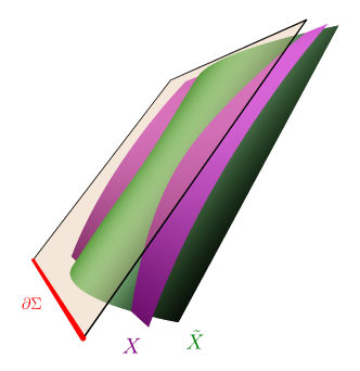
Figure 2: Two different choices of stretched horizons are shown, as the level sets of the functions $X$ and $\tilde{X}$, which lead to different scaling frames for $l_{a}$ on the null surface.

We mentioned in section 3.1 that fixing $l_{a}$ corresponds to a type of frame choice. Here, we will relate this choice to the arbitrariness in choosing a sequence of stretched horizons that approach the null surface. A stretched horizon for a null surface plays a similar role to an asymptotic cutoff surface when discussing asymptotic infinity. These are especially relevant in AdS/CFT, where different choices of the radial cutoff correspond to different conformal frames in the dual theory. This then strengthens the relation between the scaling frame for $l_{a}$ and the choice of conformal frame for the degrees of freedom associated with the quasilocal charges.

To see the relation, we let $X$ denote a function whose level sets define the sequence of stretched horizons approaching $\mathcal{N}$ at $X=0$. We let $l_{a}$ be the (unnormalized) normal form to the $X$ foliation,

$$l_{a}=\nabla_{a}X,$$ (3.37)

which is spacelike for $X>0$ and null at $X=0$. Any reparameterization of the form $X\rightarrow\tilde{X}(X)$ defines the same foliation, and its effect on the normal is simply to rescale $l_{a}$ by $\tilde{F}^{\prime}(X)$. Hence $l_{a}$ at $\mathcal{N}$ only rescales by a constant $\tilde{X}^{\prime}(0)$. We therefore see that the scaling frame of $l_{a}$ is determined by the choice of stretched horizon foliation, up to overall constant rescalings.

A different foliation of stretched horizons can be obtained by reparameterizing by an arbitrary function of the coordinates $X\rightarrow\tilde{X}(X,x^{i})$, subject to the constraint $\tilde{X}(0,x^{i})=0$, so that the foliation still approaches $\mathcal{N}$ (see figure 2). The null normal is now rescaled by the position dependent function $\partial_{X}\tilde{X}(0,x^{i})$, corresponding to a change of scaling frame.

4 Virasoro symmetry

As an application of the null boundary covariant phase space we have just constructed, we now specialize to the case of bifurcate, axisymmetric Killing horizons. These have been the subject of many previous analyses, in which quasilocal charge algebras have been used to derive expressions for the entropy of the Killing horizon [4, 10, 27, 29, 32, 84]. The standard procedure is to find a set of vector fields in the near-horizon region whose Lie brackets yield one or two copies of the Witt algebra. Upon computing the quasilocal charge algebra, one generally finds a central extension. The resulting Virasoro algebra is the symmetry algebra of a 2D CFT, suggesting that the quantization of the near horizon charge algebra should have a CFT description. The asymptotic density of states in such a theory is controlled by the Cardy formula, and by applying it in conjunction with the central charge computed from the quasilocal charge algebra, one arrives at the Bekenstein-Hawking entropy.

This procedure for arriving at the horizon entropy has been applied in a variety of different situations, often differing in the precise details of which symmetry algebra is used and what boundary conditions are imposed [5, 8, 9, 85, 11]. Here, by means of example, we provide evidence for the claim that the central charge occurring in these setups is always computed by the general formula (2.32) in terms of the noncovariance of the boundary Lagrangian for the null surface. The example we will analyze is the set of symmetry generators found for axisymmetric Killing horizons in [34], which generalize the near horizon conformal symmetries of the Kerr black hole proposed by Haco, Hawking, Perry, and Strominger (HHPS) [10]. We show that the null surface Wald-Zoupas construction described above produces a formula for the central charge which, via the Cardy formula, leads to an entropy that is twice the Bekenstein-Hawking entropy of the horizon. We argue that this factor of 2 could arise if the central charge was sensitive to both sets of edge modes, one on either side of the bifurcation surface, coupled together by the Dirichlet flux matching condition. To make a contradistinction, we compare to the case where boundary conditions are found to make the quasilocal charges integrable, and show that a different central charge results, and no factor of 2 appears. This thereby gives a derivation of the appropriate “counterterms” (i.e. fluxes) that had previously been conjectured to be necessary for the construction in [10, 34].

4.1 Near-horizon expansion

We begin by reviewing the expansion of the metric near a bifurcate Killing horizon, following a construction of Carlip [29, 34]. Let $l^{a}$ be the horizon-generating Killing vector, which is timelike in the exterior region, and becomes the null normal on the bifurcate Killing horizon $\mathcal{H}$. A canonical choice of radial vector can be made using the gradient of the norm of $l^{a}$,

$$\rho^{a}=-\frac{1}{2\kappa}\nabla^{a}\left(l\cdot l\right),$$ (4.1)

where $\kappa$ is the surface gravity, which is constant on account of the zeroth law of black hole mechanics [86]. The normalization of $\rho^{a}$ is chosen so that it coincides with $l^{a}$ on $\mathcal{H}$, and as a consequence of Killing’s equation, one finds that $l\cdot\rho=0$ and $[l,\rho]=0$ everywhere. If in addition the horizon is axisymmetric, meaning it possesses a rotational Killing vector $\psi^{a}$ that commutes with $l^{a}$, it follows that $\psi\cdot\rho=0$ and $[\psi,\rho]=0$. This allows us to choose coordinates $(t,r_{*},\phi)$ such that $(l^{a},\rho^{a},\psi^{a})$ are the corresponding coordinate basis vectors, and in this coordinate system, $g_{tr_{*}}=g_{\phi r_{*}}=0$. The radial coordinate $r_{*}$ is analogous to the tortoise coordinate in the Schwarzschild solution, with the horizon positioned at $r_{*}\rightarrow-\infty$. The remaining coordinates will be denoted $\theta^{A}$.

One can demonstrate that the norm of the radial vector near the horizon satisfies [29]

$$\rho\cdot\rho=-\left(l\cdot l\right)+\mathcal{O}\left[\left(l\cdot l\right)^{2}\right],$$ (4.2)

and hence as a function of $r_{*}$, the Killing vector norm satisfies the differential equation

$$\partial_{r_{*}}\left(l\cdot l\right)=\rho^{a}\nabla_{a}\left(l\cdot l\right)=2\kappa\left(l\cdot l\right)+\mathcal{O}\left[\left(l\cdot l\right)^{2}\right]$$ (4.3)

whose solution is

$$\left(l\cdot l\right)=-e^{2\kappa r_{*}}+\mathcal{O}\left[e^{4\kappa r_{*}}\right],$$ (4.4)

where the integration constant has been absorbed by the shift freedom in the definition of the tortoise coordinate, $r_{*}\rightarrow r_{*}+f(\theta^{A})$. This behavior suggests a reparameterization of the radial coordinate,

$$x=\frac{1}{\kappa}e^{\kappa r_{*}},\quad\implies\quad\partial_{x}^{a}=\frac{1}{\kappa x}\rho^{a}$$ (4.5)

in terms of which the Killing vector norm has the expansion

$$\left(l\cdot l\right)=-\kappa^{2}x^{2}+\mathcal{O}\left[x^{4}\right].$$ (4.6)

This also implies that $\partial_{x}^{a}$ is unit normalized to leading order in the near-horizon expansion, which means $x$ coincides with the radial geodesic distance to the bifurcation surface at this order. This fully determines the $x$ coordinate, and in terms of it, the near-horizon metric exhibits a Rindler-like expansion,

$$ds^{2}=-\kappa^{2}x^{2}dt^{2}+dx^{2}+\psi^{2}d\phi^{2}+q_{AB}d\theta^{A}d\theta^{B}-2x^{2}\kappa dt\left(N_{\phi}d\phi+N_{A}d\theta^{A}\right)+\ldots$$ (4.7)

where the $\ldots$ denotes higher order terms which do not play a role in the remainder of the analysis of the near horizon symmetries. Here, we have used the shift freedom $\phi\rightarrow\phi+G(\theta^{A})$ to eliminate any $d\phi d\theta^{A}$ terms that generically appear.

The Rindler coordinates degenerate on the future and past horizons, so it is useful to define Kruskal coordinates which are regular on the horizon,

$$U =-xe^{-\kappa t}$$ (4.8a)

$$V =xe^{\kappa t},$$ (4.8b)

in terms of which the metric becomes

$$ds^{2}=-dUdV+\psi^{2}d\phi^{2}+q_{AB}d\theta^{A}d\theta^{B}+(UdV-VdU)(N_{\phi}d\phi+N_{A}d\theta^{A})+\ldots$$ (4.9)

The Killing vector and radial vector have simple expressions in terms of Kruskal coordinates,

$$l^{a} =\kappa(V\partial_{V}^{a}-U\partial_{U}^{a})$$ (4.10)

$$\rho^{a} =\kappa(V\partial_{V}^{a}+U\partial_{U}^{a}),$$ (4.11)

which demonstrates that near the bifurcation surface at $U=V=0$, $l^{a}$ acts like a boost while $\rho^{a}$ acts like a dilatation.

The future horizon $\mathcal{H}^{+}$ in Kruskal coordinates is located at $U=0$, and on the horizon the generator is $l^{a}=\kappa V\partial_{V}^{a}$. The natural choice of auxiliary null covector there is then $n_{a}=-\frac{1}{\kappa V}\nabla_{a}V+\frac{1}{2}\left|\frac{dV}{\kappa V}\right|^{2}l_{a}$, where the term proportional to $l_{a}$ just ensures that $n_{a}$ is null on all of $\mathcal{H}^{+}$. The spacetime volume form is given by

$$\epsilon=\frac{1}{2}dU\wedge dV\wedge\mu=-l\wedge\eta,$$ (4.12)

where the induced volume form on the horizon is

$$\eta=\frac{1}{\kappa V}dV\wedge\mu.$$ (4.13)

The past horizon $\mathcal{H}^{-}$ is at $V=0$, where the generator is $l^{a}=-\kappa U\partial_{U}^{a}$ and the auxiliary null covector is $n_{a}=\frac{1}{\kappa U}\nabla_{a}U+\frac{1}{2}\left|\frac{dU}{\kappa U}\right|^{2}l_{a}$. The conventions we use to define the volume forms are slightly different than on the future horizon. We choose the volume form on the past horizon to be

$$\eta=-\frac{1}{\kappa U}dU\wedge\mu,$$ (4.14)

to maintain the relationship $\mu=i_{l}\,\eta$. This means that the spacetime volume is related to $\eta$ on the past horizon by

$$\epsilon=l\wedge\eta,$$ (4.15)

and these conventions ensure that $\mu$ limits to the same volume form on the bifurcation surface when approached on $\mathcal{H}^{+}$ or on $\mathcal{H^{-}}$. Because of (4.15), the decomposition of ${\bm{\theta}}$ picks up an overall minus sign relative to the expression (3.23). This means that on $\mathcal{H}^{-}$, the boundary term has a relative minus sign compared to (3.27)

$$\ell=\frac{k\eta}{8\pi G}\qquad(\text{on $\mathcal{H}^{-}$}).$$ (4.16)

4.2 Expression for the noncovariance

The results of section 2.3 show that any extension of the quasilocal symmetry algebra is determined by the noncovariance of the boundary term, $\Delta_{\hat{\xi}}\ell$. The noncovariance of this quantity and the various other structures defined on a generic null surface were determined in section 3.4 in terms of the scalar $w_{\xi}$ which shows up in the noncovariance of the normal form to the horizon, $l_{a}$. To apply these formulas in computations of the algebra extensions, we therefore need an expression for $w_{\xi}$ on a Killing horizon.

This can be derived on $\mathcal{H}^{+}$ by first noting that if $\xi^{a}$ is tangent to the null surface $\mathcal{N}=\mathcal{H}^{+}$, the value of $\pounds_{\xi}l_{a}$ does not depend on how $l_{a}$ is chosen away from $\mathcal{N}$. Since $l_{a}$ and $\rho_{a}$ coincide on $\mathcal{N}$, we can compute $w_{\xi}l_{a}=\pounds_{\xi}l_{a}\mathrel{\mathop{\widehat{=}}}\pounds_{\xi}\rho_{a}=\nabla_{a}(\xi\cdot\rho)$, since $(d\rho)_{ab}=0$ due to its definition as a gradient in equation (4.1). To continue the calculation, we express $\xi^{a}$ in terms of the basis $(l^{a},\rho^{a},\psi^{a},\partial_{A}^{a})$ as $\xi^{a}=\xi^{\rho}\rho^{a}+V^{a}$, where $V^{a}$ is some combination of $l^{a}$, $\psi^{a}$, and $\partial_{A}^{a}$. Since $l\cdot\rho=\psi\cdot\rho=0$ everywhere, and $\partial_{A}\cdot\rho=\mathcal{O}[x^{3}]$, when evaluated on the horizon, only the $\xi^{\rho}$ component survives in the gradient. Hence we find, using (4.2),

$$\nabla_{a}(\xi\cdot\rho)\mathrel{\mathop{\widehat{=}}}\xi^{\rho}\nabla_{a}(\rho\cdot\rho)\mathrel{\mathop{\widehat{=}}}-\xi^{\rho}\nabla_{a}\left(l\cdot l\right)\mathrel{\mathop{\widehat{=}}}2\kappa\xi^{\rho}\,l_{a}.$$ (4.17)

This leads to the simple expression,

$$w_{\xi}=2\kappa\xi^{\rho}\qquad\text{(on $\mathcal{H}^{+}$)},$$ (4.18)

so we see that the noncovariance comes entirely from the dilatation component of $\xi^{a}$, i.e. the component parallel to $\rho^{a}$. Note that although $w_{\xi}$ does not depend on how $l_{a}$ is extended off of $\mathcal{N}$, it does depend on the extension of $\xi^{a}$ in the vicinity of $\mathcal{N}$. To demonstrate this point, we note that because $l^{a}$ and $\rho^{a}$ coincide on $\mathcal{N}$, one cannot separate $\xi^{a}$ into its $l^{a}$ and $\rho^{a}$ components using its value on $\mathcal{N}$ alone. Only after looking at its behavior as you move away from $\mathcal{N}$ can its $l^{a}$ and $\rho^{a}$ components be distinguished, and then only the $\rho^{a}$ component contributes to the noncovariance.

The analysis on the past horizon $\mathcal{H}^{-}$ is similar and leads to

$$w_{\xi}=2\kappa\xi^{\rho}\qquad\text{(on $\mathcal{H}^{-}$)}.$$ (4.19)

4.3 Virasoro vector fields

Having introduced the near-horizon expansion of the metric, we now turn to the choice of vector fields generating the near-horizon symmetries. Motivated by the hidden conformal symmetry of scattering amplitudes in Kerr [31], HHPS proposed a set of vector fields for Kerr black holes whose algebra consisted of two commuting copies of the Witt algebra. This algebra was identified by foliating the near-horizon region by approximately $\text{AdS}_{3}$ slices, and writing down the corresponding asymptotic symmetry generators. The construction of these symmetry generators was extended to Schwarzschild black holes in [87], which also proposed a two-parameter generalization in the choice of vector fields, with the two parameters coinciding with notions of left and right temperatures. The construction was further extended to arbitrary axisymmetric Killing horizons in [34], which similarly identified an algebra $\text{Diff}(S^{1})_{\alpha}\times\text{Diff}(S^{1})_{\bar{\alpha}}$, consisting of two commuting copies of the Witt algebra, and labeled by two parameters $(\alpha,\bar{\alpha})$ which coincide with choices of temperatures. In this section, we will analyze this latter algebra for general choices of $(\alpha,\bar{\alpha})$, and show in section 4.4 that the quasilocal charge algebra leads to an expression for the central charges.

One way to describe the symmetry algebra is to present it in terms of a geometric structure that it preserves. To this end, we define the following “conformal coordinates” depending on the two parameters $(\alpha,\bar{\alpha})$ [34]:

$$W^{+} =Ve^{\alpha\phi}$$ (4.20a)

$$W^{-} =-Ue^{\bar{\alpha}\phi}$$ (4.20b)

$$y =e^{\frac{\alpha+\bar{\alpha}}{2}\phi}.$$ (4.20c)

The $2\pi$ periodicity of $\phi$ requires that these coordinates be identified according to $(W^{+},W^{-},y)\sim(e^{2\pi\alpha}W^{+},e^{2\pi\bar{\alpha}}W^{-},e^{\pi(\alpha+\bar{\alpha})}y)$. We then form the following tensor

$$C_{ab}=-\frac{1}{y^{2}}\nabla_{a}W^{+}\,\nabla_{b}W^{-}=\Big{(}\nabla_{a}V+\alpha V\nabla_{a}\phi\Big{)}\Big{(}\nabla_{b}U+\bar{\alpha}U\nabla_{b}\phi\Big{)}$$ (4.21)

where the second equality demonstrates that $C_{ab}$ is well-defined in light of the periodicity of the conformal coordinates. The near-horizon symmetries are defined to simply be the transformations that preserve $C_{ab}$. A trivial set of such transformations are simply those parallel to the transverse directions, $V^{A}\partial_{A}$. They preserve the bifurcation surface of the horizon, and hence do not require the Wald-Zoupas prescription, nor do they lead to algebra extensions when represented in terms of quasilocal charges. We therefore focus on the nontrivial transformations that act in the $(t,r_{*},\phi)$ plane.

Using the first expression for $C_{ab}$ in (4.21), it is straightforward to see that the vector fields that satisfy $\pounds_{\xi}C_{ab}=0$ are of the form

$$\xi^{a}_{n} =F_{n}(W^{+})\partial_{+}^{a}+\frac{1}{2}F_{n}^{\prime}(W^{+})y\partial_{y}^{a}$$ (4.22)

$$\bar{\xi}^{a}_{n} =\bar{F}_{n}(W^{-})\partial_{-}^{a}+\frac{1}{2}\bar{F}^{\prime}_{n}(W^{-})y\partial_{y}^{a}.$$ (4.23)

In order to be single-valued, the functions $F_{n},\bar{F}_{n}$ must satisfy $F_{n}(W^{+}e^{2\pi\alpha})=F_{n}(W^{+})e^{2\pi\alpha}$, $\bar{F}_{n}(W^{-}e^{2\pi\bar{\alpha}})=\bar{F}_{n}(W^{-})e^{2\pi\bar{\alpha}}$, and hence they can be expanded in modes,

$$F_{n} =\alpha W^{+}\left(W^{+}\right)^{\frac{in}{\alpha}}$$ (4.24)

$$\bar{F}_{n} =-\bar{\alpha}W^{-}\left(W^{-}\right)^{-\frac{in}{\bar{\alpha}}}.$$ (4.25)

We can then compute the Lie brackets of these vector fields, and find that their algebra is given by two commuting copies of the Witt algebra,

$$[\xi_{m},\xi_{n}] =i(n-m)\xi_{m+n}$$ (4.26)

$$[\bar{\xi}_{m},\bar{\xi}_{n}] =i(n-m)\bar{\xi}_{m+n}$$ (4.27)

$$[\xi_{m},\bar{\xi}_{n}] =0$$ (4.28)

Although preservation of the tensor $C_{ab}$ uniquely specifies the near-horizon symmetry generators, there is still a question as to why this is a useful criterion to impose. While we do not have a completely satisfactory answer, we can point out some interesting features of $C_{ab}$ that may inform future investigations into its significance. First we note that the vector fields also preserve the following contravariant tensor,

$$D^{ab}=-y^{2}\partial_{+}^{a}\partial_{-}^{b}=\partial_{V}^{a}\partial_{U}^{b}=\frac{1}{2\kappa^{2}x^{2}}(l^{a}+\rho^{a})(l^{b}-\rho^{b}),$$ (4.29)

for any choice of $(\alpha,\bar{\alpha})$. From this, one can also construct the projectors

$$(P_{+})\indices{{}^{b}_{a}} =C_{ac}D^{bc}=\nabla_{a}W^{+}\partial^{b}_{+}=\left(\frac{\nabla_{a}V}{\kappa V}+\frac{\alpha}{\kappa}\nabla_{a}\phi\right)\kappa V\partial_{V}^{b}$$ (4.30)

$$(P_{-})\indices{{}^{b}_{a}} =C_{ca}D^{cb}=\nabla_{a}W^{-}\partial_{-}^{b}=\left(\frac{\nabla_{a}U}{\kappa U}+\frac{\bar{\alpha}}{\kappa}\nabla_{a}\phi\right)\kappa U\partial_{U}^{b}$$ (4.31)

which are also preserved. On $\mathcal{H^{+}}$, the upper index of $(P_{+})\indices{{}^{a}_{b}}$ is parallel to the horizon generator, and so by pulling back the lower index to $\mathcal{H^{+}}$, one arrives at a vertical projector for vectors on $\mathcal{H^{+}}$ onto $l^{a}$. Such a projector is an example of an Ehresmann connection for the horizon, viewed as a fiber bundle with fibers consisting of the null flow lines of $l^{a}$. It is, in fact, a flat connection, with horizontal directions given by the surfaces of constant $W^{+}$. However, this connection produces a nontrivial holonomy upon completing a $2\pi$ rotation in $\phi$, which results in $V\rightarrow Ve^{-2\pi\alpha}$ (see [34] for a depiction of this spiraling behavior of the conformal coordinates). $(P_{-})\indices{{}^{a}_{b}}$ similarly defines a flat Ehresmann connection on the past horizon, with $2\pi$ holonomy $U\rightarrow Ue^{-2\pi\bar{\alpha}}$.

The relevance of such Ehresmann connections in the study of Carroll geometries on null surfaces [88] was recently emphasized in [89], so investigating the relationship between Carroll geometries and the near-horizon Virasoro symmetries may lead to a deeper understanding as to their fundamental origin. Note, however, it is important that the generators are defined to preserve $C_{ab}$ in a neighborhood of the bifurcation surface; it is not enough to simply find vector fields that preserve $P_{+}$ and $P_{-}$ on each of the respective horizons. This is because the behavior of $\xi^{a}_{n}$ off of the horizon determines the noncovariances, which in turn determine extensions of the quasilocal charge algebra. Since $C_{ab}$ contains the information about both projectors, the geometric interpretation of the symmetry generators seems to involve not only the Ehresmann connections on each individual horizon, but also how they relate to each other in forming a bifurcate horizon.

As discussed in section 4.2, the noncovariances depend on the $\rho^{a}$ component of the symmetry generators. This can be computed by transforming the vector fields (4.22) and (4.23) back to the $(t,r_{*},\phi)$ coordinate system, in which they are expressed in terms of $l^{a}$, $\rho^{a}$, and $\psi^{a}$. Using (4.5), (4.8), and (4.20), this leads to

$$\xi_{n}^{a} =\frac{\left(W^{+}\right)^{\frac{in}{\alpha}}}{\alpha+\bar{\alpha}}\left[\frac{\alpha\bar{\alpha}}{\kappa}l^{a}+\alpha\psi^{a}+in\left(\frac{\bar{\alpha}-\alpha}{2\kappa}l^{a}+\psi^{a}\right)\right]-\frac{in}{2\kappa}\left(W^{+}\right)^{\frac{in}{\alpha}}\rho^{a}$$ (4.32)

$$\bar{\xi}_{n}^{a} =\frac{\left(W^{-}\right)^{-\frac{in}{\bar{\alpha}}}}{\alpha+\bar{\alpha}}\left[\frac{\alpha\bar{\alpha}}{\kappa}l^{a}-\bar{\alpha}\psi^{a}+in\left(\frac{\bar{\alpha}-\alpha}{2\kappa}l^{a}+\psi^{a}\right)\right]-\frac{in}{2\kappa}\left(W^{-}\right)^{-\frac{in}{\bar{\alpha}}}\rho^{a},$$ (4.33)

Note that the prefactor $\left(W^{+}\right)^{\frac{in}{\alpha}}=V^{\frac{in}{\alpha}}e^{in\phi}$ in $\xi_{n}^{a}$ has an oscillating singularity as the past horizon at $V\rightarrow 0$ is approached. This means that the $\xi_{n}^{a}$ vector fields have no well-defined limit to the past horizon, and so their quasilocal charges will be constructed on the future horizon. Similarly, the prefactor $\left(W^{-}\right)^{-\frac{in}{\bar{\alpha}}}=(-U)^{-\frac{in}{\bar{\alpha}}}e^{-in\phi}$ in $\bar{\xi}_{n}^{a}$ has no limit to the future horizon $U\rightarrow 0$, and so the corresponding quasilocal charges will be evaluated on $\mathcal{H}^{-}$. With this in mind, we can read off the expression for the noncovariances associated with these vector fields using (4.18) and (4.19), which gives

$$w_{\xi_{n}} =-in\left(W^{+}\right)^{\frac{in}{\alpha}}\qquad\text{(on $\mathcal{H^{+}}$)}$$ (4.34)

$$w_{\bar{\xi}_{n}} =-in\left(W^{-}\right)^{-\frac{in}{\bar{\alpha}}}\qquad\text{(on $\mathcal{H^{-}}$)}.$$ (4.35)

We now demonstrate that these vector fields do not preserve the boundary conditions $\delta k=0$, $\delta l^{a}\mathrel{\mathop{\widehat{=}}}0$, or $n_{a}\delta l^{a}\mathrel{\mathop{\widehat{=}}}0$ that have been employed in previous works [17, 19, 78, 79]. On $\mathcal{H}^{+}$,

$$I_{\hat{\xi}_{n}}\delta k =-n(n-i\alpha)\frac{\kappa}{\alpha}\left(W^{+}\right)^{\frac{in}{\alpha}},$$ (4.36)

$$I_{\hat{\xi}_{n}}\delta l^{a} =\frac{n(n-i\alpha)}{\alpha+\bar{\alpha}}\left(W^{+}\right)^{\frac{in}{\alpha}}\left[-l^{a}+\frac{\kappa}{\alpha}\psi^{a}\right],$$ (4.37)

which clearly violates all three conditions pointwise. These conditions are also violated pointwise by the $\bar{\xi}_{n}^{a}$ generators on $\mathcal{H}^{-}$,

$$I_{\hat{\bar{\xi}}_{n}}\delta k =-n(n+i\bar{\alpha})\frac{\kappa}{\bar{\alpha}}\left(W^{-}\right)^{-\frac{in}{\bar{\alpha}}}$$ (4.38)

$$I_{\hat{\bar{\xi}}_{n}}\delta l^{a} =\frac{n(n+i\bar{\alpha})}{\alpha+\bar{\alpha}}\left(W^{-}\right)^{-\frac{in}{\bar{\alpha}}}\left[l^{a}+\frac{\kappa}{\bar{\alpha}}\psi^{a}\right].$$ (4.39)

This therefore necessitates the use of the weaker boundary conditions described in section 3.2.

4.4 Central charges

With all this in place, we can proceed to the calculation of the central extension of the quasilocal charge algebra. We denote the quasilocal charges for $\xi_{n}^{a}$ by $L_{n}$, and the charges for $\bar{\xi}_{n}^{a}$ by $\bar{L}_{n}$. Their values are given by the general expression (2.20), evaluated on $\mathcal{H}^{+}$ for the $L_{n}$ generators and on $\mathcal{H}^{-}$ for the $\bar{L}_{n}$ generators. Note that because the background is rotationally symmetric, all of the charges $L_{n}$, $\bar{L}_{n}$ except for $L_{0}$, $\bar{L}_{0}$ vanish, since the generators (4.32), (4.33) come with angular dependence $e^{in\phi}$, which integrates to zero on $\partial\Sigma$. Of course, their variations, which enter the calculation of the brackets, need not vanish. Since the vector fields $\xi_{0}^{a}$ and $\bar{\xi}_{0}^{a}$ are linear combinations of the horizon-generating and rotational Killing vectors, $l^{a}$ and $\psi^{a}$, the $L_{0}$, $\bar{L}_{0}$ charges will be linear combinations of the Noether charges for the Killing vectors, namely, the horizon area $A$ and angular momentum $J_{H}$. The zero mode generators evaluate to

$$L_{0} =\frac{\alpha}{\alpha+\bar{\alpha}}J_{H}$$ (4.40)

$$\bar{L}_{0} =-\frac{\bar{\alpha}}{\alpha+\bar{\alpha}}J_{H},$$ (4.41)

where the horizon angular momentum $J_{H}$ is given by the Noether charge for the rotational Killing vector $\psi^{a}$,

$$J_{H}=\int_{\partial\Sigma}Q_{\psi}=\frac{1}{4G}\int d\theta^{A}\sqrt{q}|\psi|N_{\phi}(\theta^{A}).$$ (4.42)

The area contribution has dropped from these expressions because the quasilocal charge $H_{l}$ for $l^{a}$, which normally is proportional to the area, vanishes upon including the Dirichlet boundary term $i_{l}\ell$ from (2.20). This is somewhat unintuitive because $l^{a}$ vanishes as the bifurcation surface is approached; however, the contraction with $\ell$ has a nonzero value in the limit. The vanishing of this boost Noether charge was similarly observed in the analysis of a phase space bounded by a timelike hypersurface with Dirichlet boundary conditions [37, 63].

The discussion of section 2.3 showed that the Barnich-Troessaert bracket of the charges must reproduce the algebra of the vector fields, up to abelian extensions. Hence, for the $\xi_{n}^{a}$ vector fields, the bracket of the charges can be written

$$\{L_{m},L_{n}\}=-i\Big{[}(n-m)L_{m+n}+K_{m,n}\Big{]},$$ (4.43)

where $K_{m,n}$ is determined by the explicit formula (2.32),

$$K_{m,n}=-i\int_{\partial\Sigma}\Big{(}i_{\xi_{m}}\Delta_{\hat{\xi}_{n}}\ell-i_{\xi_{n}}\Delta_{\hat{\xi}_{m}}\ell\Big{)}.$$ (4.44)

To evaluate this, we first note that the expression (3.36) for the noncovariance of $k\eta$ and the expression (4.34) for $w_{\xi_{n}}$ gives

$$\Delta_{\hat{\xi}_{n}}\ell=\frac{\eta}{8\pi G}l^{a}\nabla_{a}w_{\xi_{n}}=\frac{\eta}{8\pi G}\frac{n^{2}\kappa}{\alpha}\left(W^{+}\right)^{\frac{in}{\alpha}}.$$ (4.45)

For the quantity $i_{\xi_{m}}\eta$, note that the $\psi^{a}$ component will not contribute to this expression when evaluated on a surface of constant $V$. Recalling that $\rho^{a}=l^{a}$ on $\mathcal{H^{+}}$, we have

$$i_{\xi_{m}}\eta=\frac{\left(W^{+}\right)^{\frac{in}{\alpha}}}{\alpha+\bar{\alpha}}\left(\frac{\alpha\bar{\alpha}}{\kappa}-im\frac{\alpha}{\kappa}\right)i_{l}\eta=\frac{\left(W^{+}\right)^{\frac{in}{\alpha}}}{\alpha+\bar{\alpha}}\frac{\alpha}{\kappa}\left(\bar{\alpha}-im\right)\mu.$$ (4.46)

Then we find that

$$i_{\xi_{m}}\left(\Delta_{\hat{\xi}_{-m}}\ell\right)=-im^{2}\frac{(m+i\bar{\alpha})}{(\alpha+\bar{\alpha})}\frac{\mu}{8\pi G},$$ (4.47)

and subtracting the term with $m\leftrightarrow-m$ and integrating over the surface gives a result proportional to the horizon area $A$,

$$K_{m,-m}=\frac{A}{4\pi G(\alpha+\bar{\alpha})}m^{3}.$$ (4.48)

Any other extension term $K_{m,n}$ with $m\neq-n$ vanishes, again due to rotational invariance and the overall $e^{-i(m-n)\phi}$ dependence of the integrand. We verify in appendix D that the variations of the quantities $K_{m,n}$ with $m\neq-n$ are consistent with having identically zero quasilocal charges associated with them, which means that the only nontrivial extension terms are $K_{m,-m}$. Hence, the extension is in fact central, and the algebra obtained is the Virasoro algebra,

$$\{L_{m},L_{n}\}=-i\Big{[}(n-m)L_{m+n}+\frac{c}{12}m^{3}\delta_{m,-n}\Big{]}$$ (4.49)

with central charge

$$c=\frac{3A}{\pi G(\alpha+\bar{\alpha})}.$$ (4.50)

The analysis for the $\bar{\xi}_{n}^{a}$ generators is similar. The calculations need to be done on the past horizon due to the singularity in $\bar{\xi}_{n}^{a}$ on the future horizon. As explained in section 4.1, this flips the sign of the boundary term $\ell$ in the decomposition of the symplectic form. This then gives

$$\Delta_{\hat{\bar{\xi}}_{n}}\ell =-\frac{\eta}{8\pi G}l^{a}\nabla_{a}w_{\bar{\xi}_{n}}=-\frac{\eta}{8\pi G}\frac{n^{2}\kappa}{\bar{\alpha}}\left(W^{-}\right)^{-\frac{in}{\bar{\alpha}}}$$ (4.51)

$$i_{\bar{\xi}_{n}}\eta =\frac{\left(W^{-}\right)^{-\frac{in}{\bar{\alpha}}}}{\alpha+\bar{\alpha}}\frac{\bar{\alpha}}{\kappa}(\alpha+in)\mu$$ (4.52)

$$i_{\bar{\xi}_{m}}\left(\Delta_{\hat{\bar{\xi}}_{-m}}\ell\right) =-im^{2}\frac{(m-i\alpha)}{(\alpha+\bar{\alpha})}\frac{\mu}{8\pi G}$$ (4.53)

From this last expression, we can compute the extension

$$\bar{K}_{m,-m} =-i\int_{\partial\Sigma}\Big{(}i_{\bar{\xi}_{m}}\Delta_{\hat{\bar{\xi}}_{-m}}\ell-i_{\bar{\xi}_{-m}}\Delta_{\hat{\bar{\xi}}_{m}}\ell\Big{)}$$ (4.54)

$$=\frac{A}{4\pi G(\alpha+\bar{\alpha})}m^{3}.$$ (4.55)

As before, the $\bar{L}_{n}$ generators are then seen to satisfy a Virasoro algebra with central charge

$$\bar{c}=\frac{3A}{\pi G(\alpha+\bar{\alpha})},$$ (4.56)

which is the same value as $c$ given in (4.50). Note that $c,\bar{c}$ given in (4.50), (4.56) are twice the values computed in [34, 10]. This factor of 2 will have an effect on the entropy computed in section 5.1.

4.5 Frame dependence

Although the null normal is fixed to coincide with the Killing horizon generator in the definition of the near-horizon phase space, we would like to understand how the central charges depend on the choice of background scaling frame. This is relevant because the choice of frame was related to the choice of stretched horizon in section 3.5, and since this frame has parallels to a choice of Weyl frame in a CFT, we would like the central charge to be insensitve to this choice. Under the rescaling transformation (3.1), the parameter $w_{\xi}$ characterizing the noncovariance of $l_{a}$ transforms according to

$$w_{\xi}\rightarrow w_{\xi}+\pounds_{\xi}f.$$ (4.57)

Using (3.36), this then leads to a change in the anomaly of the boundary term by

$$\Delta_{\hat{\xi}}\ell\rightarrow\Delta_{\hat{\xi}}\ell-\frac{\eta}{8\pi G}\pounds_{l}\pounds_{\xi}f.$$ (4.58)

For the $\xi_{n}^{a}$ generators on $\mathcal{H}^{+}$, this results in an extra contribution to $K_{m,-m}$ given by the integral over the bifurcation surface of the following quantity:

$$\frac{\mu}{2\pi G}\frac{m}{(\alpha+\bar{\alpha})^{2}}\left[\alpha(m^{2}+\bar{\alpha}^{2})V\frac{\partial f}{\partial V}+\frac{\partial}{\partial\phi}\left((\alpha\bar{\alpha}-m^{2})f+(\alpha+\bar{\alpha})\frac{\partial f}{\partial V}\right)\right].$$ (4.59)

The term involving a total $\phi$ derivative integrates to zero, and hence does not affect the central charge. The term that can affect the result is the one proportional to $V\frac{\partial f}{\partial V}$ in the limit $V\rightarrow 0$. If $f$ is a regular function of $V$ at $V=0$, this term drops out and the central charge is unaffected. To get a nonzero contribution from it, we would need $f\sim\lambda\log V$, corresponding to a rescaling of $l^{a}$ by $V^{\lambda}$. This then affects the rate at which $l^{a}$ vanishes (or blows up) as the bifurcation surface is approached. For example, given the form of $l^{a}$ in (4.10), we see that $\lambda=-1$ rescales $l^{a}$ to an affine parameterization, since $V$ is an affine parameter.

In order to arrive at an unambiguous value of the central charge, we must disallow transformations that affect the rate at which $l^{a}$ vanishes as $V\rightarrow 0$. This means choosing a normalization so that it vanishes linearly with respect to an affine parameter as bifurcation surface is approached, just as the horizon-generating Killing vector does. Note that this still allows for rescalings of the generator in a $\phi$ or $\theta^{A}$-dependent manner, or, relatedly, making a different choice of the affine parameter with respect to which $l^{a}$ vanishes linearly. However, it rules out using an affinely parameterized generator when analyzing bifurcate null horizons. Using the Killing parameterization of the null generator is natural for Killing horizons, but it may be that other choices are preferred for different setups. Note that in [10, 34], it seems that a nonstandard choice of this normalization was used, which happened to set any contribution to the central charge from the flux to zero except the Hájíček term. It would be interesting to explore these other normalizations in more detail in the future.

5 Entropy from the Cardy formula

The relevance of equations (4.50) and (4.56) for the central charges is that they contain information about the entropy of the horizon. To see how this comes about, we need to associate a quantum system with the near-horizon degrees of freedom. It is well known that in a theory with gauge symmetry such as general relativity, the introduction of a spatial boundary breaks some of the gauge invariance, thereby producing additional degrees of freedom on the boundary that would otherwise not have been present [25, 24, 7]. The edge modes that arise in this fashion are acted on by the quasilocal charges identified in the previous sections, and thus represent a classical system with Virasoro symmetry. The quantization of this system should respect the symmetry, and since two dimensional conformal field theories share this symmetry algebra, we are led to the postulate that the quantum system should be a 2D CFT. In such a theory, the asymptotic density of states depends in a universal way on the central charge according to the Cardy formula [30]. We will find that applying this formula in the context of a Killing horizon shows that the entropy of the CFT is directly related to the entropy of the horizon.

5.1 Canonical Cardy formula

The Cardy formula comes in two flavors: microcanonical and canonical. The canonical formula applies to a CFT in a thermal state at high temperatures, and states that the entropy is given by

$$S_{\text{Cardy}}=\frac{\pi^{2}}{3}(c\,T+\bar{c}\,\bar{T}),$$ (5.1)

where $T$ and $\bar{T}$ are known as the left and right temperatures; they are the thermodynamic potentials conjugate to the $L_{0}$ and $\bar{L}_{0}$ charges.

To apply this formula in the context of a Killing horizon, we need to identify the temperatures. This can be done in a manner similar to the determination of the Hawking temperature in terms of the horizon surface gravity. We would expect the density matrix for quantum fields just outside of the horizon to be in the Frolov-Thorne vacuum [32, 90, 33], which is thermal with respect to the horizon-generating Killing vector $l^{a}$. This means the density matrix should be of the form

$$\rho\sim e^{-\frac{2\pi}{\kappa}\omega_{l}},$$ (5.2)

where $\omega_{l}=-k_{a}l^{a}$ is the frequency of a mode with wavevector $k_{a}$, relative to $l^{a}$, and the coefficient $\frac{2\pi}{\kappa}$ is the inverse Hawking temperature. Since $l^{a}$ can be expressed in terms of the left and right Virasoro vector fields via $\frac{1}{\kappa}l^{a}=\frac{1}{\alpha}\xi_{0}^{a}+\frac{1}{\bar{\alpha}}\bar{\xi}_{0}^{a}$, the density matrix can equivalently be written

$$\rho\sim e^{-\frac{2\pi}{\alpha}\omega_{0}-\frac{2\pi}{\bar{\alpha}}\bar{\omega}_{0}}$$ (5.3)

where now $\omega_{0}=-k_{a}\xi^{a}_{0}$, $\bar{\omega}_{0}=k_{a}\bar{\xi}^{a}_{0}$ are the frequencies with respect to the Virasoro zero mode generators. This then leads us to identify the left and right temperatures

$$T=\frac{\alpha}{2\pi},\qquad\bar{T}=\frac{\bar{\alpha}}{2\pi}.$$ (5.4)

With these temperatures in hand, the Cardy formula (5.1) applied using the computed values (4.50), (4.56) for $c,\bar{c}$ yields

$$S_{\text{Cardy}}=2\left(\frac{A}{4G}\right).$$ (5.5)

Somewhat unexpectedly, we arrive at twice the entropy of the horizon. To interpret this result, recall that the central charges were computed using the Barnich-Troessaert bracket of quasilocal charges. This bracket was employed because the quasilocal charges are not integrable, since they are associated with evolution up the horizon, during which symplectic flux leaks out. In order to justify such a calculation, one should introduce an auxiliary system that collects the lost symplectic flux, allowing integrable generators and Poisson brackets to be defined on the total system. Since we postulated that the edge modes on one side of the horizon are described by a 2D CFT, it is equally natural to assume that the auxiliary system is another copy of the same CFT, associated with edge modes on the other side of the horizon. This is the picture that would appear when cutting a global Cauchy surface for the full spacetime across the bifurcation surface, in which case the left wedge and its edge modes are the only additional degrees of freedom in the space, and hence must comprise the auxiliary system that collects the fluxes from the right wedge. If we assume that the Barnich-Troessaert bracket computes the central charge of the total system, we would arrive at twice the value of the central charge for one of the CFTs. This would explain the appearance of the factor of 2 in (5.5), since it is counting the entropy associated with edge modes on both sides of the horizon. If we then traced out the auxiliary system, we would expect the entropy to be exactly half the value computed above, and hence would arrive at the correct horizon entropy,

$$S=\frac{A}{4G}.$$ (5.6)

This conjectural resolution will be expanded upon in section 6.2. In order to support this interpretation by way of contrast, we turn now to a case where the quasilocal charges are in fact integrable, so that no fluxes or auxiliary systems are needed.

5.2 Integrable charges

The other possibility that would produce the correct entropy is if the boundary term $\ell$ were half the value given in equation (3.27). This would correspond to different boundary conditions than Dirichlet, since the flux would now contain an additional contribution proportional to $\delta k$. Although this appears unnatural from the perspective of gluing subregions discussed in section 2.2, if we were only interested in integrable charges so that the subregion could be treated as a closed system, any boundary condition that results in integrability is valid. In this section, we will show that such modified boundary conditions are necessary if demanding that the HHPS charges be integrable.

A useful property of the Barnich-Troessaert bracket is that if boundary conditions are imposed to make the charges integrable, it reduces to the Dirac bracket of these charges on the submanifold of phase space defined by imposing the boundary conditions as constraints. The integrable charges therefore need not be considered quasilocal, but rather are legitimate Hamiltonians generating the symmetry on the constrained phase space. Note, however, that the vector fields generating the symmetry must preserve the boundary condition imposed, i.e. they must be tangent to the constraint submanifold, since otherwise they do not produce well-defined transformations of the constrained fields.

Finding a boundary condition that ensures vanishing symplectic flux but is also preserved by the vector fields (4.32) and (4.33) is somewhat nontrivial, since the vector fields tend to violate any local condition fixing the intrinsic or extrinsic quantities on the horizon, see equations (4.36), (4.37), (4.38), and (4.39). However, as discussed in [34], one can consider more general conditions that are preserved by the symmetry generators, involving integrals of variations of quantities over portions of the horizon. Assuming such a condition is found, the fact that the fluxes then vanish consequently implies that the bracket $\{L_{n},L_{-n}\}$ can be computed simply from contracting the vector fields $\hat{\xi}_{n}$, $\hat{\xi}_{-n}$ into the symplectic form $\Omega$. This computation was already performed in [34], and the resulting central charges are

$$c =\frac{24}{(\alpha+\bar{\alpha})^{2}}\left(\frac{\bar{\alpha}A}{8\pi G}+J_{H}\right)$$ (5.7)

$$\bar{c} =\frac{24}{(\alpha+\bar{\alpha})^{2}}\left(\frac{\alpha A}{8\pi G}-J_{H}\right).$$ (5.8)

On the other hand, the general formula (2.32) for the extension in terms of $\Delta_{\hat{\xi}}\ell$ still remains valid, albeit with a possibly different choice of boundary term than $\ell=\frac{-k}{8\pi G}\eta$. The simplest generalization is to take

$$\ell=\frac{-ak}{8\pi G}\eta,$$ (5.9)

with $a$ some constant. In order to ensure that the values of $L_{0}$ and $\bar{L}_{0}$ are the same when computed on either the future or past horizon, we must then choose the boundary term on the past horizon to be $\frac{ak}{8\pi G}\eta$. Doing this produces the central charges

$$c=\bar{c}=\frac{3aA}{\pi G(\alpha+\bar{\alpha})}.$$ (5.10)

Equating the above two expressions for $c$ and $\bar{c}$ yields the conditions

$$\alpha-\bar{\alpha}=\frac{16\pi GJ_{H}}{A},\qquad a=\frac{1}{2}.$$ (5.11)

The first condition restricts the parameters $\alpha,\bar{\alpha}$ defining the symmetry generators, and was identified in [34] as a necessary condition for integrability of the charges. The second condition $a=\frac{1}{2}$ shows that the boundary term $\ell$ is half of the value used when imposing a Dirichlet flux condition. It implies that the central charges are now half of the value computed in section 4.4,

$$c=\bar{c}=\frac{3A}{2\pi G(\alpha+\bar{\alpha})},$$ (5.12)

and consequently the entropy coming from the canonical Cardy formula (5.1) now agrees with the horizon entropy,

$$S_{\text{Cardy}}=\frac{A}{4G}.$$ (5.13)

5.3 Microcanonical Cardy formula

The canonical Cardy formula requires the left and right temperatures as inputs, which were identified for the horizon using properties of the Frolov-Thorne vacuum for quantum fields outside of the horizon. A more microscopic derivation of the entropy would utilize the microcanonical Cardy formula, which expresses the entropy in terms of the density of states at fixed, large values of $L_{0}$, $\bar{L}_{0}$. The microcanonical expression for the entropy is

$$S_{\mu\text{Cardy}}=2\pi\left(\sqrt{\frac{cL_{0}}{6}}+\sqrt{\frac{c\bar{L}_{0}}{6}}\right).$$ (5.14)

To apply this formula, we need the values of the charges $L_{0}$ and $\bar{L}_{0}$. Note that we should expect the microcanoncial formula to work only in the case that the charges are integrable, since only then do $L_{0}$, $\bar{L}_{0}$ represent global charges for a closed system. This is consistent with standard thermodynamics, in which the microcanonical ensemble counts the number of states within a fixed energy band of a closed system, while the canonical ensemble is used for an open system interacting with a bath at fixed temperature.

According to the discussion in section 5.2, integrability of the charges requires that the boundary term $\ell$ be on future horizon

$$\ell=-\frac{k\eta}{16\pi G},$$ (5.15)

and the past horizon expression is just $\ell=\frac{k\eta}{16\pi G}$, which are half the values they take under Dirichlet flux matching. This boundary term enters explicitly into the expression for the charges via equation (2.20), and making the choice (5.15) is important for finding the right entropy from the microcanonical Cardy formula.

Including the contribution from the boundary term (5.15), we now find that the zero mode charges are

$$L_{0} =\frac{\alpha}{\alpha+\bar{\alpha}}\left(\frac{\bar{\alpha}A}{16\pi G}+J_{H}\right)=\frac{\alpha^{2}}{(\alpha+\bar{\alpha})}\frac{A}{16\pi G}$$ (5.16)

$$\bar{L}_{0} =\frac{\bar{\alpha}}{\alpha+\bar{\alpha}}\left(\frac{\alpha A}{16\pi G}-J_{H}\right)=\frac{\bar{\alpha}^{2}}{(\alpha+\bar{\alpha})}\frac{A}{16\pi G},$$ (5.17)

where the latter equalities in these equations employ the integrability condition (5.11) determining $\alpha-\bar{\alpha}$. Using these values in the microcanonical Cardy formula (5.14) with the central charges (5.12) gives

$$S_{\mu\text{Cardy}}=\frac{A}{4G},$$ (5.18)

in agreement with the canonical result (5.13) and coinciding with the horizon entropy.

6 Discussion

In this work, we revisited the Wald-Zoupas construction of quasilocal charges and fluxes for subregions with null boundaries, with the goal of systematically deriving the central charges that have appeared in several recent works on symmetries near Killing horizons [10, 35, 11, 87, 34, 36]. This required generalizing the treatment in [17] of the Wald-Zoupas procedure for null boundaries by allowing for the most general boundary conditions consistent with the presence of a null hypersurface. In the process, we arrived at a general formula (2.32) for the algebra extension that appears in the quasilocal charge algebra, which would be applicable in other investigations of near horizon symmetries. We showed that the central charge arises from fixing $l_{a}$ as the background structure, which we related to a choice of stretched horizon. In this context, the central charge arises as an anomaly, in a manner quite analogous to the holographic Weyl anomaly appearing in AdS/CFT due to noncovariance of the gravitational action under changes in the radial cutoff. Applying the Cardy formula to the central charges of a bifurcate, axisymmetric Killing horizon obtained using the Dirichlet flux condition yielded twice the entropy of the horizon, and we argued that the factor of $2$ could be indicative of a complementary set of edge modes on the other side of the horizon. We now expand upon the possible significance of these results, and end with some future directions.

6.1 Algebra extension as a scaling anomaly

The formula (2.32) for the algebra extension $K_{\xi,\zeta}$ shows that extensions only arise when the boundary term $\ell$ is not covariant with respect to the transformations generated by $\xi^{a}$, $\zeta^{a}$. In several other treatments of symmetries at null boundaries, the boundary term was chosen to be covariant, and equation (2.32) therefore explains the vanishing of the central extensions in those cases [17, 19, 21]. The fact that the extension is always of the form of a trivial field-dependent cocycle [43] given by equation (2.36), means that the boundary term can always be chosen to be covariant so as to eliminate the extension $K_{\xi,\zeta}$. However, such a choice is in conflict with the Dirichlet form of the flux, and hence describes a physically different setup. Put another way, there is nontrivial physics in the choice of boundary term, and we should not view different choices of this term as a type of gauge freedom.

By imposing the Dirichlet flux condition, we were inevitably led to fluxes and boundary terms that were not covariant under the boundary symmetries. This noncovariance seems to be a feature, rather than a bug, as it gives rise to the central charge which ultimately accounts for the horizon entropy. The source of noncovariance came from fixing a choice of the null normal $l_{a}$. This can be viewed as a choice of frame, since there is generally no preferred normalization of $l_{a}$ when the surface is null. The choice of $l_{a}$ bears resemblance to the choice of radial cutoff when describing asymptotic symmetries, or, equivalently, the choice of conformal factor when dealing with the conformal compactification. In holographic renormalization, the appearance of conformal anomalies in the dual CFT is known to be related to anomalous transformations of boundary terms in the gravitational action with respect to the radial cutoff [44, 45, 46, 47, 91]. Changing the radial cutoff then affects the induced metric in the limit that the conformal boundary is approached, and hence coincides with a choice of Weyl frame in the CFT.

To strengthen the analogy between this notion of conformal frame and the scaling frame of $l_{a}$, we showed in section 3.5 that a preferred normalization of $l_{a}$ is determined if one specifies a sequence of stretched horizons that asymptote to the null surface. As has been remarked before, there are multiple ways to stretch the horizon [92], and here we see that this ambiguity has a precise analog in terms of the scaling frame of $l_{a}$. Furthermore, the ambiguity in stretching the horizon, or equivalently, choosing the scaling frame of $l_{a}$, is actually responsible for the appearance of the central charges in the horizon symmetry algebra. The radial vector $\rho^{a}$ introduced in equation (4.1) generates transformations that change the stretched horizon foliation pointwise, acting like a dilatation about the bifurcation surface. Intriguingly, we showed in section 4.2 that the $\rho^{a}$ component of the symmetry generators is solely responsible for producing anomalous transformations of objects on the horizon. This suggests that $\rho^{a}$ should be thought of as generating changes in the scaling frame of the horizon CFT, just as the radial vector in AdS generates Weyl transformations for the holographic CFT. The central charge in the horizon quasilocal charge algebra appears as a classical diffeomorphism anomaly coming from $\Delta_{\hat{\xi}}\ell$, and experience with holographic anomalies tells us that it should be interpreted as a quantum anomaly in a dual quantum description [44, 45, 46, 47]. The Virasoro central charge indeed has this interpretation in 2D CFTs, where it appears as an anomaly in the CFT stress tensor [93].

The interpretation of the central charge as an anomaly may help explain why computations involving the Cardy formula do such a good job of capturing the black hole entropy. It is somewhat surprising that a set of Virasoro symmetry generators appear for Killing horizons of arbitrary dimension, when standard holographic reasoning would suggest that a higher dimensional CFT should appear for higher dimensional black holes. It is also surprising that seemingly disparate symmetry algebras, including $\text{BMS}_{3}$ [5, 9, 85], Virasoro-Kač-Moody [11], Heisenberg [8], or just a single copy of Virasoro [4, 29], all seem to reproduce the black hole entropy when a Cardy-like formula is available, even though each of these symmetries would coincide with physically different quantum theories. Some insight into this situation comes from recalling that the Cardy formula is derived using the anomalous tranformation of the stress tensor when performing a change in conformal frame from the plane to the cylinder [94, 30]. The conformal anomaly determines the vacuum expectation value of the stress tensor, which is attributed to a Casimir energy associated with putting the theory on a cylinder. Modular invariance then relates this vacuum energy to the high temperature density of states, from which one arrives at the Cardy formula for a CFT. The central charge appears in this formula in its capacity as an anomaly coefficient, and it may be that this conformal anomaly controls the density of states in more general contexts when an exact 2D CFT description is not valid. In such a scenario, the extension in the quasilocal algebra would continue to characterize the rescaling anomaly, and one might hope that a suitable generalization of the Cardy formula would still reproduce the black hole entropy. Note, however, that modular invariance is a crucial input in the derivation of the Cardy formula, and hence it should play an important role in arriving at the correct entropy.

6.2 Barnich-Troessaert bracket and Dirichlet matching

The Barnich-Troessaert bracket given in (2.28) played an important role in defining the algebra satisfied by the quasilocal charges. As of yet, however, there is no derivation of this bracket from first principles. The main technical problem is in coming up with an object which replaces the Poisson bracket when dealing with an open subsystem, which can lose symplectic flux through a boundary. There has been some work addressing this problem for general phase spaces with boundaries [96, 97, 98, 99], but it remains to be seen exactly the connection between these works and the present context of quasilocal charges in gravity. The heuristic derivation of the bracket in section 2.3 describes how it might arise by including an auxiliary system which collects the lost symplectic flux, but it would clearly be interesting to carry out such a construction in full detail.

A step toward deriving the Barnich-Troessaert bracket was taken by Troessaert in [72], who interpreted the quasilocal symmetry transformations in terms of a family of phase spaces parameterized by a set of boundary sources. These boundary sources are simply the values taken by the fields appearing in the flux. For the Dirichlet form of the flux the, intrinsic metric $q_{ij}$ and null generator $l^{i}$ constitute the sources. This interpretation is inspired by holography, where the holographic dictionary relates boundary values of the fields to sources in the dual CFT, and their conjugate momenta to expectation values of the sourced operators [100, 101]. In this case, the momenta $\pi^{ij}$ and $\pi_{i}$ from equations (3.29) and (3.30) should have the interpretation of the holographic stress tensor for the null boundary, similar to the Brown-York stress tensor on the timelike boundary in standard examples of AdS/CFT [45]. Dirichlet conditions also play an important role in holography, since other boundary conditions can lead to conformal field theories with fluctuating sources or metrics, whose interpretation as a well-defined theory is less clear [83]. Troessaert describes the quasilocal symmetries as “external symplectic symmetries,” which are transformations that act on the boundary sources as well as the dynamical fields, and demonstrates that the Barnich-Troessaert bracket arises in a natural way on this enlarged phase space. External symplectic symmetries have also appeared in the context of asymptotically flat spaces, where superrotations have been shown to be of this character [102].

The interpretation of the Barnich-Troessaert bracket in terms of an enlarged phase space decomposed into smaller phase spaces of fixed Dirichlet field values is similar to the description of fixed area states in holography [103, 104]. Specifically, in the latter construction, a bulk Cauchy slice is split across the Ryu-Takayanagi (RT) surface [105, 106], and a general state in the gravitational Hilbert space is decomposed into superselection sectors corresponding to area eigenstates of the RT surface, each of which classically corresponds to a fixed Dirichlet boundary condition (albeit for a codimension-two boundary as opposed to a codimension-one boundary). This description in terms of fixed area states was important for reproducing the correct Renyi spectrum of holographic states. The analogue of the external symplectic transformations are operators that belong to neither the algebra of the entanglement wedge nor its complement. In other words, such transformations would not preserve the center. Fixed area states appeared earlier in a slightly different context in [40], where it was argued that the Bekenstein-Hawking entropy arises from summing over all fixed area configurations of a black hole in Euclidean gravity. Therefore, it might not be all that coincidental that we needed to fix the Dirichlet form in the symplectic potential in order to reproduce the Bekenstein-Hawking entropy from the Cardy formula; investigating the connection between the present work and these other works would be an interesting next step.

Ultimately, the Barnich-Troessaert bracket should arise from a Poisson bracket on a larger phase space, consisting of a subregion and its complement. When gluing together the two subregion phase spaces to construct the global phase space, each choice for the form of the flux $\mathcal{E}$ corresponds to a specific matching of the boundary variables. As discussed in section 2.2, the Dirichlet flux is used to kinematically match the metric on the dividing surface, while the discontinuity in momenta $\pi^{ij}$ and $\pi_{i}$ are dynamically set equal to the boundary stress energy by the combined variational principle for the subregion and its complement, yielding a version of the junction conditions for general relativity [69, 70, 107]. Matching the intrinsic data is preferred over matching the momenta, since jumps in intrinsic data lead to distributionally ill-defined curvatures, which we expect to be excluded from the gravitational path integral. In a complete derivation of the Barnich-Troessaert bracket, we therefore expect the Dirichlet flux condition to play an important role.

6.3 Edge modes and the factor of 2

A surprising result of this work is the appearance of the additional factor of $2$ in the central charges (4.50), (4.56) and entropy (5.5) when using the Dirichlet flux condition to define the quasilocal charges. This hints at the existence of a pair of CFTs describing the degrees of freedom near the horizon. The gluing picture described in section 6.2 supports this interpretation, since in such a description, one would naturally construct a pair of quasilocal charge algebras before combining them into a global phase space. Once this procedure is carried out, it may be that the Barnich-Troessaert bracket computes the algebra associated with the global Virasoro charges of the two CFTs combined, which would lead to a central charge that is twice the value associated with the single CFT on one side. The canonical Cardy formula then returns the total entropy assuming the CFT is in a global thermal state, but if we are interested in the entropy associated only with degrees of freedom outside of the horizon, we would first have to trace out the additional interior degrees of freedom. This would have the effect of halving the value of the entropy obtained, which leads to the correct entropy formula, $S=\frac{A}{4G}$.

A contrasting setup was analyzed in sections 5.2 and 5.3, in which the quasilocal charges were specialized to integrable ones. This required a different boundary term that resulted in central charges and an entropy that were both half the values obtained using the Dirichlet flux, and hence correctly gave the horizon entropy. Integrability of the charges allows the subregion to be viewed as a closed system, in which case the central charge we compute would have to be associated with only a single CFT. A further consistency check in this case was agreement with the microcanonical Cardy formula, which holds since the system is isolated. The interpretation of the Dirichlet matching condition then seems to be that it necessarily entails a description in terms of an open system, and the Barnich-Troessaert bracket computes the total central charge associated with both sets of quasilocal charges. On the other hand, the boundary term necessary for integrable charges seems to be associated with one-sided generators, which, at least for the special choice of parameters given in equation (5.11), do not require a gluing construction. Of course, it may be that there is some other justification for using the alternative boundary term over the Dirichlet one in a gluing construction, and it would be interesting to explore this possibility further.

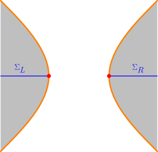
(a) Subregions before gluing

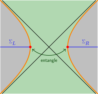
(b) Connected geometry after gluing

Figure 3: Depiction of the gluing procedure. In (3(a)) we show two disconnected subregions, bounded by timelike stretched horizons in orange. The boundaries of the respective Cauchy surfaces $\Sigma_{L}$ and $\Sigma_{R}$ are given by the red dots. In (3(b)), we imagine gluing the subregions by entangling the edge modes on $\partial\Sigma_{L}$ with those on $\partial\Sigma_{R}$. This entanglement should build up the geometry of the intervening space. For the nonextremal horizons considered in this paper, the stretched horizons can approach the bifurcate null horizon, and the gluing occurs accross the bifurcation surface, with the entanglement building up the geometry of the interior.

This picture in terms of a pair of CFTs arises naturally when interpreting the horizon entropy as an entanglement entropy. In a theory with gauge symmetry such as general relativity, the quantum mechanical Hilbert space does not factorize into a tensor product associated with a subregion and its complement. However, one can form an extended Hilbert space [108] that does factorize by introducing additional edge mode degrees of freedom on the boundary which are acted on by a quasilocal charge algebra closely related to the ones considering in the present work [26, 7]. The physical Hilbert space is then identified with a particular subspace of the extended Hilbert space, which is constructed in a way analogous to the gluing construction described above. This gluing procedure produces entanglement between the edge modes, which ultimately contributes to the entropy of the state [108], and in some cases can be the dominant contribution.

In the context of this work, since the quasilocal symmetries contain a Virasoro algebra, we expect each set of edge modes to be described in terms of a CFT. In order to apply the Cardy formula, this CFT must be modular-invariant, which is an additional assumption beyond requiring that the edge mode theory furnish a representation of the Virasoro algebra. In fact, if one worked with an irreducible representation of Virasoro, the density of states would grow like a CFT with central charge $c=1$, which is clearly insufficient to reproduce the horizon entropy. A possible way to view the effect of modular invariance on the edge mode description is to think of it as an additional symmetry that acts on the edge modes, which then implies additional degeneracy of the states when the edge mode theory is quantized. This additional dengeneracy coming from modular invariance appears to be important for arriving at the correct value of the Bekenstein-Hawking entropy.

The gluing procedure for the edge modes should entangle the pair of CFTs at the boundaries into something like a thermofield double state. This creates a picture that is quite familiar from holography, where entanglement between a pair of CFTs builds up a connected black hole geometry in the bulk [109, 110, 111] (see figure 3). The difference when working on the horizon is that when gluing at the bifurcation surface, the two sets of edge modes are coincident, as opposed to being spatially separated by the AdS interior. Nevertheless, one might attribute the smooth region to the future of the bifurcation surface as arising from the edge mode entanglement, similar to how smooth bulk geometries arise from entanglement in holography. If one instead worked on the stretched horizons, there would be a small spatial region between the gluing surfaces which could be thought of as built up from edge mode entanglement.

In a limit where the horizon approaches extremality with $\kappa\rightarrow 0$, the stretched horizon picture begins to look like standard derivations of holographic dualities [112, 113]. The additional ingredient in AdS/CFT is the appearance of a long AdS throat, separating the stretched horizon from what would have been a bifurcation surface, were it not infinitely far away. Associated with this throat is the existence of a decoupling limit between modes deep within the throat and excitations in the distant asymptotically flat region, which allows the CFT dual to the AdS throat to be treated as a closed system. This decoupling limit is not available for the nondegenerate horizons considered in this paper, and the CFT associated with the quasilocal charges must be thought of as interacting with degrees of freedom in the exterior. The need to employ the Wald-Zoupas procedure due to the presence of fluxes can be viewed as an indication of this lack of decoupling. Although nonstandard in traditional treatments of AdS/CFT, recent works on black hole evaporation in holography have employed a similar setup, where the standard Dirichlet boundary conditions in AdS are relaxed to allow fluxes of Hawking radiation to escape into an auxiliary asymptotically flat region [114, 115]. Time translation in such a setup should then be viewed as an external symplectic symmetry of the AdS subregion, and the definitions of energy and the boundary symmetry algebra would require the Wald-Zoupas procedure and the Barnich-Troessaert bracket. Understanding the quasilocal symmetry algebras of horizons may therefore provide additional insights into the black hole evaporation process and information paradox.

6.4 Future work

This work raises a number of questions that motivate further investigation. Foremost amongst these is the interpretation of the Barnich-Troessaert bracket and its relation to the gluing of subregions. Deriving the bracket from a gluing construction would make progress towards confirming the conjectured origin of the factor of 2 appearing in the central charge with Dirichlet flux matching. Beyond that, the gluing construction would demonstrate a way to describe a localized subregion in gravity, from which one could ask additional questions about local gravitational observables. On the quantum side, this gluing procedure gives a way to embed the global gauge-invariant Hilbert space of the theory into an extended Hilbert space, and allows notions of entanglement entropy for a subregion to be defined. It should also have a description in terms of the sewing of path integrals [40, 116, 117], which may also lead to further justifications of the Dirichlet matching condition.

Although the main application of this work was an analysis of the Virasoro vector fields for Killing horizons, the general formalism we developed is much more broadly applicable. In particular, the expression (2.32) for the central extension in terms of the anomalous transformation of the boundary term in the action applies quite generally, and hence can be utilized for a variety of symmetry algebras and types of hypersurfaces. One interesting application would be to investigate the various extended symmetry algebras that have been proposed for asymptotically flat space with these methods [13, 14, 118, 16, 119]. In particular, there may be some connection between the null boundary stress tensor we found in this paper and the celestial stress tensor found for 4D asymptotically flat spaces in [120], although we expect that suitable counterterms to regulate this expression will be needed [65, 67]. It would also be interesting to explore the relation between these boundary terms and fluxes and the recent work on effective actions for superrotation modes [121].

More generally, one could look at symmetry algebras associated with arbitrary null surfaces [17, 21], and analyze the extensions that appear using the Dirichlet flux condition. One intriguing aspect of some of these symmetry algebras is that they include factors of $\text{Diff}(S^{2})$, which is known to have no nontrivial central extensions. However, the Barnich-Troessaert bracket generically produces abelian extensions, which do exist for $\text{Diff}(S^{2})$. It would be interesting to see if these extensions have any connection to anomalies in a putative quantum description, and whether one can find a Cardy-like formula related to the abelian extensions.

In [17] a BMS-like algebra was found on arbitrary null surfaces, which can be written as a semidirect sum $\text{diff}(S^{2})\ltimes\mathfrak{s}$, where $\mathfrak{s}$ consists of the generators of the form $\xi^{a}=fl^{a}$. As discussed in section 3.2, [17] employed the boundary condition $\delta k=0$, which constrains the function $f$ to satisfy $\pounds_{l}(\pounds_{l}+k)f=0$, so these generators form a pointwise $\mathbb{R}\ltimes\mathbb{R}$ subalgebra corresponding to position-dependent translations and boosts along the null surface, the former of which correspond to supertranslations. We can readily see from our general expression (2.32) along with the choice of boundary term (3.27) on a null surface that the $\delta k=0$ boundary condition makes the central charge trivially vanish. As explained in [17], if we lift the $\delta k=0$ condition, then the only modification to the algebra is that now $f$ can be any function on the null surface; such vector fields were considered for example in [21]. In particular, if we consider two generators $\xi^{a}=fl^{a}$ and $\tilde{\xi}^{a}=\tilde{f}l^{a}$, the extension $K_{\xi,\tilde{\xi}}$ computed from (2.32) will be nonzero for an arbitary null surface. A step towards understanding the universality of the Bekenstein-Hawking entropy from the Cardy formula would therefore entail a better understanding of this enlargement of the $\mathbb{R}\ltimes\mathbb{R}$ subalgebra and the resulting abelian extension.

The Wald-Zoupas construction we described in this work required the symmetry generators to be tangent to a hypersurface that bounds the subregion of interest. However, diffeomorphisms which move the bounding hypersurface should also possess quasilocal charges. Treating such transformations would require additional analysis of the decomposition of the symplectic potential at the null surface, and a characterization of the noncovariances that can arise from such transformations, but in principle a similar set of techniques should allow quasilocal charges to be defined for these surface deformations. Carrying this out in detail would be a useful next step.

Another generalization would be to investigate higher curvature theories using the Wald-Zoupas procedure. We anticipate this being more challenging due to the presence of higher time derivatives in the action. In particular, we should not expect the Dirichlet flux condition to be available in general, with the exception of Lovelock theories, for which the null boundary terms corresponding to Dirichlet conditions are known [122]. Determining a suitable generalization of that condition would be the main obstacle one would need to overcome. The analysis of [123] on near horizon symmetries of extremal black holes in higher curvature theories may give some insights into this problem.

Finally, an open question related to the Virasoro symmetry generators considered in [10] is with regards to their geometrical significance. In the extremal limit, the generators become symmetries of a warped $\text{AdS}_{3}$ throat [32, 33], but away from extremality their interpretation is less clear. In [31], the parameters $\alpha$ and $\bar{\alpha}$ were determined by a hidden conformal symmetry of the scalar wave equation in the near-horizon region. Determining how this symmetry relates to preservation of the tensor $C_{ab}$ defined in (4.21) would lead to further insights on the relation between the near-horizon Virasoro generators and null boundary data.

Appendix A Commutation relation for anomaly operator

Here, we give a proof of the relation (2.2) satisfied by the anomaly operator $\Delta_{\hat{\xi}}$. By writing out the commutator, we find

$$[\Delta_{\hat{\xi}},\Delta_{\hat{\zeta}}]=[L_{\hat{\xi}},L_{\hat{\zeta}}]+[\pounds_{\xi},\pounds_{\zeta}]-[L_{\hat{\xi}},\pounds_{\zeta}]-[\pounds_{\xi},L_{\hat{\zeta}}]=L_{[\hat{\xi},\hat{\zeta}]_{\mathcal{S}}}+\pounds_{[\xi,\zeta]}.$$ (A.1)

Here, $[\hat{\xi},\hat{\zeta}]_{\mathcal{S}}$ is the Lie bracket of vector fields on $\mathcal{S}$, and to arrive at the second equality, we use the fact that $[L_{\hat{\xi}},\pounds_{\zeta}]$ = 0, since $\zeta^{a}$ is field-independent, $\delta\zeta^{a}=0$. The field space bracket can be related to the spacetime bracket simply by contracting with a covariant field $\delta g_{ab}$,

$$I_{[\hat{\xi},\hat{\zeta}]_{\mathcal{S}}}\delta g_{ab} =L_{\hat{\xi}}I_{\hat{\zeta}}\delta g_{ab}-I_{\hat{\zeta}}L_{\hat{\xi}}\delta g_{ab}=L_{\hat{\xi}}\pounds_{\zeta}g_{ab}-I_{\hat{\zeta}}\pounds_{\xi}\delta g_{ab}=\pounds_{\zeta}\pounds_{\xi}g_{ab}-\pounds_{\xi}\pounds_{\zeta}g_{ab}=-\pounds_{[\xi,\zeta]}g_{ab}$$

$$=-I_{\widehat{[\xi,\zeta]}}\delta g_{ab},$$ (A.2)

and hence we derive

$$[\hat{\xi},\hat{\zeta}]_{\mathcal{S}}=-\widehat{[\xi,\zeta]}$$ (A.3)

for field-independent generators. Applying this to (A.1) yields the desired identity

$$[\Delta_{\hat{\xi}},\Delta_{\hat{\zeta}}]=-\Delta_{\widehat{[\xi,\zeta]}}.$$ (A.4)

It is also useful to note the commutators with $L_{\hat{\zeta}}$ and $\pounds_{\zeta}$,

$$[\Delta_{\hat{\xi}},L_{\hat{\zeta}}] =-L_{\widehat{[\xi,\zeta]}}$$ (A.5)

$$[\Delta_{\hat{\xi}},\pounds_{\zeta}] =-\pounds_{[\xi,\zeta]}.$$ (A.6)

Appendix B Derivation of the bracket identity

Here, we derive the main identity for the Barnich-Troessaert bracket and the resulting extension $K_{\xi,\zeta}$. To be completely general, we do not assume that $\Delta_{\hat{\xi}}\beta=0$. We first work with the definition (2.20) of the quasilocal charges, so that all of $\Delta_{\hat{\xi}}\beta$ is contained in the flux. The Barnich-Troessaert bracket is then

$$\{H_{\xi},H_{\zeta}\}=I_{\hat{\xi}}\delta H_{\zeta}-\int_{\partial\Sigma}\Big{(}i_{\xi}I_{\hat{\zeta}}\mathcal{E}-I_{\hat{\zeta}}\Delta_{\hat{\xi}}\beta\Big{)}\equiv\int_{\partial\Sigma}m_{\xi,\zeta},$$ (B.1)

where we have written the final result in terms of a local 2-form $m_{\xi,\zeta}$ to be integrated. We can calculate the expression for $m_{\xi,\zeta}$ on $\mathcal{N}$ as follows:

$$m_{\xi,\zeta} =I_{\hat{\xi}}\delta Q_{\zeta}+I_{\hat{\xi}}i_{\zeta}\delta\ell-I_{\hat{\xi}}\delta I_{\hat{\zeta}}\beta-i_{\xi}I_{\hat{\zeta}}{\bm{\theta}}-i_{\xi}I_{\hat{\zeta}}\delta\ell+I_{\hat{\zeta}}i_{\xi}d\beta+I_{\hat{\zeta}}\Delta_{\hat{\xi}}\beta$$

$$=-Q_{[\xi,\zeta]}+i_{\xi}dQ_{\zeta}-i_{\xi}I_{\hat{\zeta}}{\bm{\theta}}+i_{\zeta}\Delta_{\hat{\xi}}\ell-i_{\xi}\Delta_{\hat{\zeta}}\ell+i_{\zeta}\pounds_{\xi}\ell-i_{\xi}\pounds_{\zeta}\ell-L_{\hat{\xi}}I_{\hat{\zeta}}\beta+I_{\hat{\zeta}}L_{\hat{\xi}}\beta$$

$$\qquad\qquad+d\left(i_{\xi}Q_{\zeta}-i_{\xi}I_{\hat{\zeta}}\beta\right)$$

$$=-Q_{[\xi,\zeta]}-i_{[\xi,\zeta]}\ell+I_{\widehat{[\xi,\zeta]}}\beta-i_{\xi}\Delta_{\hat{\zeta}}\ell+i_{\zeta}\Delta_{\hat{\xi}}\ell-i_{\xi}i_{\zeta}(L+d\ell)+d\left(i_{\xi}Q_{\zeta}+i_{\xi}i_{\zeta}\ell-i_{\xi}I_{\hat{\zeta}}\beta\right)$$ (B.2)

where the first equality used the relation (2.14) for $\mathcal{E}$, the second equality expanded the variation of $Q_{\zeta}$ via

$$I_{\hat{\xi}}\delta Q_{\zeta}=L_{\hat{\xi}}Q_{\zeta}=\pounds_{\xi}Q_{\zeta}+\Delta_{\hat{\xi}}Q_{\zeta}=i_{\xi}dQ_{\zeta}+di_{\xi}Q_{\zeta}-Q_{[\xi,\zeta]},$$ (B.3)

the third equality employed the identities

$$i_{\zeta}\pounds_{\xi}\ell-i_{\xi}\pounds_{\zeta}\ell=-i_{[\xi,\zeta]}\ell+i_{\xi}i_{\zeta}d\ell+di_{\xi}i_{\zeta}\ell$$ (B.4)

and

$$-L_{\hat{\xi}}I_{\hat{\zeta}}\beta+I_{\hat{\zeta}}L_{\hat{\xi}}\beta=-I_{[\hat{\xi},\hat{\zeta}]_{\mathcal{S}}}\beta=I_{\widehat{[\xi,\zeta]}}\beta$$ (B.5)

where the $\mathcal{S}$ Lie bracket $[\hat{\xi},\hat{\zeta}]_{\mathcal{S}}$ is related to the spacetime Lie bracket for field-independent generators by a minus sign according to (A.3). By integrating (B.2) over $\partial\Sigma$, we arrive at the desired identity for the bracket,

$$\{H_{\xi},H_{\zeta}\}=-\left[H_{[\xi,\zeta]}+\int_{\partial\Sigma}\Big{(}i_{\xi}\Delta_{\hat{\zeta}}\ell-i_{\zeta}\Delta_{\hat{\xi}}\ell\Big{)}\right]$$ (B.6)

noting that the exact term in (B.2) integrates to zero and $i_{\xi}i_{\zeta}(L+d\ell)$ pulls back to zero since $\xi^{a}$ and $\zeta^{a}$ are tangent to the hypersurface $\mathcal{N}$, so their transverse components to $\partial\Sigma$ must be parallel to each other.

Note that if we examine the steps leading to (B.2), we see that the terms involving $\beta$ do not mix with the other terms, i.e. we have an independent identity involving only $\beta$,

$$-I_{\hat{\xi}}\delta I_{\hat{\zeta}}\beta+I_{\hat{\zeta}}i_{\xi}d\beta+I_{\hat{\zeta}}\Delta_{\hat{\xi}}\beta=I_{\widehat{[\xi,\zeta]}}\beta-di_{\xi}I_{\hat{\zeta}}\beta.$$ (B.7)

This immediately implies that different choices of $\beta$ in the decomposition (2.14) of ${\bm{\theta}}$ do not affect the algebra or extension $K_{\xi,\zeta}$. Stated differently, different choices of how to separate off the corner term $\beta$ from the flux $\mathcal{E}$ correspond to changes in the charges associated with trivial extensions, $H_{\xi}\rightarrow H_{\xi}+\int_{\partial\Sigma}I_{\hat{\xi}}(\beta-\beta^{\prime})$. This explains why the choice of corner term did not enter into the results for the central charges reported in [10, 34].

When utilizing the corner improvement described in appendix C, the modification of the charges and bracket amounts to shifting $\{H_{\xi},H_{\zeta}\}$ by the term,

$$-\int_{\partial\Sigma}\Big{(}I_{\hat{\xi}}\delta\Delta_{\hat{\zeta}}c-I_{\hat{\zeta}}\delta\Delta_{\hat{\xi}}c\Big{)}$$ (B.8)

with $c$ defined by equation (C.1). Then noting that the integrand can be written

$$-L_{\hat{\xi}}\Delta_{\hat{\zeta}}c+L_{\hat{\zeta}}\Delta_{\hat{\xi}}c =-\pounds_{\xi}\Delta_{\hat{\zeta}}c-\Delta_{\hat{\xi}}\Delta_{\hat{\zeta}}c+\pounds_{\zeta}\Delta_{\hat{\xi}}c+\Delta_{\hat{\zeta}}\Delta_{\hat{\xi}}c$$

$$=\Delta_{\widehat{[\xi,\zeta]}}c-i_{\xi}\Delta_{\hat{\zeta}}dc+i_{\zeta}\Delta_{\hat{\xi}}dc-d(i_{\xi}\Delta_{\hat{\zeta}}c-i_{\zeta}\Delta_{\hat{\xi}}c)$$ (B.9)

where we have applied the relation (A.4). The first term is the contribution to improved charge $-H_{[\xi,\zeta]}$, while the second and third terms correct $K_{\xi,\zeta}$, and the last term integrates to zero. This then leads to the expression (C.7) for the central charge using the corner improvement.

Finally, we verify the cocycle identity (2.35) that must be satisfied by $K_{\xi,\zeta}$. Using the expression (2.36) for $K_{\xi,\zeta}$ as a trivial field-dependent cocycle, we have

$$I_{\hat{\chi}}\delta K_{\xi,\zeta}=\int_{\partial\Sigma}\Big{(}i_{\xi}L_{\hat{\chi}}L_{\hat{\zeta}}\ell-i_{\zeta}L_{\hat{\chi}}L_{\hat{\xi}}\ell-i_{[\xi,\zeta]}I_{\hat{\chi}}\delta\ell\Big{)}$$ (B.10)

Then adding cyclic permutations we get

$$I_{\hat{\chi}}\delta K_{\xi,\zeta}+\text{cyclic}=\int_{\partial\Sigma}\Big{(}i_{\zeta}I_{\widehat{[\chi,\xi]}}\delta\ell-i_{[\chi,\xi]}I_{\hat{\zeta}}\delta\ell-i_{[\zeta,[\chi,\xi]]}\ell\Big{)}+\text{cyclic},$$ (B.11)

where we note that the cyclic contributions of the form $i_{[\zeta,[\chi,\xi]]}\ell$ actually sum to zero by the Jacobi identity. They are included to put the right hand side into the form $K_{[\chi,\xi],\zeta]}+\text{cyclic}$, which verifies the cocycle identity (2.35).

Appendix C Corner improvement

In deriving the expression (2.20) for the quasilocal charges, we assumed that the corner term was covariant, $\Delta_{\hat{\xi}}\beta=0$. Although we will find that for a null surface this condition is satisfied, it is still interesting to consider the case where the corner term is not covariant, as it leads to a useful improvement to the expression for the quasilocal charges and the extensions $K_{\xi,\zeta}$. Another reason to consider this case is to resolve an additional ambiguity that arises in the decomposition (2.14) of $\theta$. Fixing the form of $\mathcal{E}$ still allows us to make the shifts $\ell\rightarrow\ell+da$, $\beta\rightarrow\beta+\delta a$. Under this transformation, the quasilocal charge transforms as $H_{\xi}\rightarrow H_{\xi}-\int_{\partial\Sigma}\Delta_{\hat{\xi}}a$, and hence $H_{\xi}$ is sensitive to this ambiguity if $a$ is not covariant. Since we are allowing for noncovariance in $\ell$, there is no reason to assume that $\beta$ and $a$ cannot similarly be constructed from noncovariant objects.

To handle the case where $\beta$ is not covariant, we return to equation (2.19) and find that we need a way to separate $\Delta_{\hat{\xi}}\beta$ into a contribution to the charge and a contribution to the flux. Similar to how we handled $\theta$, we look for a decomposition of $\beta$ at $\partial\Sigma$ of the form

$$\beta=-\delta c+\varepsilon.$$ (C.1)

Note that this decomposition should be made on $\mathcal{N}$ without pulling back $\beta$ to $\partial\Sigma$. In principle we could also include an exact contribution $d\gamma$ in the decomposition, but these will always end up integrating to zero on $\partial\Sigma$. This decomposition allows us to identify $\varepsilon$ with a corner contribution to the flux, while $c$ is the contribution to the charge.

The improved quasilocal charge can then be written

$$H_{\xi} =\int_{\partial\Sigma}\Big{(}Q_{\xi}+i_{\xi}\ell-I_{\hat{\xi}}\beta-\Delta_{\hat{\xi}}c\Big{)}$$ (C.2)

$$=\int_{\partial\Sigma}\Big{(}Q_{\xi}-I_{\hat{\xi}}\varepsilon+i_{\xi}(\ell+dc)\Big{)}$$ (C.3)

and its variation satisfies an equation similar to (2.21),

$$\delta H_{\xi}=-I_{\hat{\xi}}\Omega+\int_{\partial\Sigma}\Big{(}i_{\xi}\mathcal{E}-\Delta_{\hat{\xi}}\varepsilon\Big{)}.$$ (C.4)

The continuity equation for the change in the charges between two cuts of $\mathcal{N}$ is

$$H_{\xi}(S_{2})-H_{\xi}(S_{1})=\int_{N^{2}_{1}}\Big{(}I_{\hat{\xi}}\mathcal{E}-\Delta_{\hat{\xi}}(\ell+dc)\Big{)},$$ (C.5)

with $F_{\xi}=\int_{\mathcal{N}_{1}^{2}}I_{\hat{\xi}}\mathcal{E}$ still interpreted as the flux, but with an anomalous source now given by $\int_{\mathcal{N}_{1}^{2}}\Delta_{\hat{\xi}}(\ell+dc)$. Finally, the Barnich-Troessaert bracket is defined for these charges as

$$\{H_{\xi},H_{\zeta}\}=-I_{\hat{\xi}}I_{\hat{\zeta}}\Omega+\int_{\partial\Sigma}\Big{(}I_{\hat{\xi}}(i_{\zeta}\mathcal{E}-\Delta_{\hat{\zeta}}\varepsilon)-I_{\hat{\zeta}}(i_{\xi}\mathcal{E}-\Delta_{\hat{\xi}}\varepsilon)\Big{)}$$ (C.6)

which again satisfies (2.31) with the extension given by

$$K_{\xi,\zeta}=\int_{\partial\Sigma}\Big{(}i_{\zeta}\Delta_{\hat{\xi}}(\ell+dc)-i_{\xi}\Delta_{\hat{\zeta}}(\ell+dc)\Big{)}.$$ (C.7)

As before, the ambiguities in the decomposition are fixed once we have specified the form of the corner flux term $\varepsilon$. We expect in this case a Dirichlet condition would fix the form of $\varepsilon$, and arguments based on the variational principle should relate the matching to codimension-2 junction conditions, such as those considered in [107]. Once this is done, the shift, $\beta\rightarrow\beta+\delta a$ causes $c\rightarrow c-a$, while $\varepsilon$ is invariant. Hence, the combination $\ell+dc$ is also insensitive to this shift, and can be viewed as the improvement to the boundary Lagrangian $\ell$ by a contribution from a corner Lagrangian $c$. We see that many of the improved formulas are obtained from those of previous sections by merely replacing $\ell$ with its invariant form, $\ell+dc$.

Note that the formula for the improved quasilocal charges (C.3) can be used even in the case that $\beta$ is already covariant. This could be useful in cases where one wishes for the corner flux to depend on the geometry of $\partial\Sigma$, in which case it will not be covariant with respect to transformations that move $\partial\Sigma$, even if $\beta$ originally was.

Appendix D Checking extension is central

As discussed in section 2.3, the Barnich-Troessaert bracket of quasilocal charges generically produces an abelian extension of the associated algebra of vector fields. We found that for the generators $\xi_{n}^{a}$ and $\bar{\xi}_{n}^{a}$, all of the extensions $K_{m,n}$ vanished in the Killing horizon background except for $K_{m,-m}$. However, the quantities $K_{m,n}$ have nonzero variations, so in principle their brackets with the $L_{n}$ generators could show that the algebra is a nontrivial abelian extension of the Witt algebra. Here we will demonstrate that in fact the extension is central, verifying that the resulting algebra is the Virasoro algebra.

The quantity to compute for $\chi^{c}$, $\xi^{c}$ and $\zeta^{c}$ three of the $\xi_{n}^{a}$ generators is (ignoring factors of $8\pi G$)

$$I_{\hat{\chi}}\delta\Big{(}i_{\xi}\Delta_{\hat{\zeta}}\ell\Big{)}=-i_{\xi}I_{\hat{\chi}}\delta\big{(}\eta l^{c}\big{)}\nabla_{c}w_{\zeta}$$ (D.1)

since $\delta w_{\zeta}=0$, which follows from $\delta w_{\zeta}l_{a}=-\delta\Delta_{\hat{\zeta}}l_{a}=\Delta_{\hat{\zeta}}\delta l_{a}=0$. Then we have

$$I_{\hat{\chi}}\delta\big{(}\eta l^{c}\big{)} =\pounds_{\chi}\big{(}\eta l^{c}\big{)}+\Delta_{\hat{\chi}}\big{(}\eta l^{c}\big{)}=(\pounds_{\chi}\eta)l^{c}+\eta\pounds_{\chi}l^{c}=(I_{\hat{\chi}}\delta\eta)l^{c}-(\Delta_{\hat{\chi}}\eta)l^{c}+\eta[\chi,l]^{c}$$

$$=\eta\Big{(}-w_{\chi}l^{c}+[\chi,l]^{c}\Big{)}$$

$$=-\eta\left(w_{\chi}l^{c}+in\frac{\kappa}{\alpha}\chi^{c}\right)$$ (D.2)

using that $\Delta_{\hat{\chi}}(\eta l^{c})=0$ for any vector that preserves the horizon, and $I_{\hat{\chi}}\delta\eta\mathrel{\mathop{\widehat{=}}}0$ for the Virasoro vector fields. The last line uses that $l^{c}=\frac{\kappa}{\alpha}\xi_{0}^{c}+\frac{\kappa}{\bar{\alpha}}\bar{\xi}_{0}^{c}$ to compute the bracket with $\chi^{c}$, and has chosen $\chi^{c}=\xi_{n}^{c}$.

Now setting $\zeta^{a}=\chi_{m}^{a}$, and using the expression (4.34) for $w_{\zeta}$, $w_{\chi}$, we have that

$$\left(w_{\chi}l^{c}+in\frac{\kappa}{\alpha}\chi^{c}\right)\nabla_{c}w_{\zeta} =-inm^{2}\frac{\kappa}{\alpha}\big{(}W^{+})^{\frac{i(m+n)}{\alpha}}+inm^{2}\frac{\kappa}{\alpha}\big{(}W^{+})^{\frac{i(m+n)}{\alpha}}=0$$ (D.3)

using that $l^{c}=\kappa V\partial_{V}^{c}$ on $\mathcal{H}^{+}$ in Kruskal coordinates (4.10), and $\chi^{c}=\alpha\big{(}W^{+}\big{)}^{\frac{in}{\alpha}}\left(W^{+}\partial_{+}^{c}+\frac{in}{2\alpha}y\partial_{y}^{c}\right)$ in conformal coordinates (4.22). This shows that the integrand in $I_{\hat{\chi}}\delta K_{\xi,\zeta}$ vanishes. According to the definition (2.33) for the Barnich-Troessaert bracket of $K_{\xi,\zeta}$ with the other generators, we see that this implies that $K_{\xi,\zeta}$ commutes with all generators, and hence must be central. Thus we arrive at the advertised result, that we have the Virasoro algebra as our extension, as opposed to some other abelian extension. The analysis on the past horizon for the $\bar{\xi}_{n}^{a}$ generator is analogous, and similarly confirms that the $\bar{L}_{n}$ generators form a Virasoro algebra.

References

- [1] S. B. Giddings, D. Marolf and J. B. Hartle, Observables in effective gravity, Phys. Rev. D 74 (2006) 064018. [arXiv:hep-th/0512200].
- [2] D. Marolf, Unitarity and Holography in Gravitational Physics, Phys. Rev. D 79 (2009) 044010. [arXiv:0808.2842].
- [3] W. Donnelly and S. B. Giddings, Diffeomorphism-invariant observables and their nonlocal algebra, Phys. Rev. D 93 (2016) . [arXiv:1507.07921].
- [4] S. Carlip, Black hole entropy from conformal field theory in any dimension, Phys. Rev. Lett. 82 (1999) 2828–2831. [arXiv:hep-th/9812013].
- [5] A. Bagchi, S. Detournay, R. Fareghbal and J. Simón, Holography of 3D flat cosmological horizons, Phys. Rev. Lett. 110 (2013) 141302. [arXiv:1208.4372].
- [6] S. W. Hawking, M. J. Perry and A. Strominger, Soft hair on black holes, Phys. Rev. Lett. 116 (2016) . [arXiv:1601.00921].
- [7] W. Donnelly and L. Freidel, Local subsystems in gauge theory and gravity, J. High Energy Phys. 2016 (2016) 1–45. [arXiv:1601.04744].
- [8] H. Afshar, S. Detournay, D. Grumiller, W. Merbis, A. Perez, D. Tempo et al., Soft Heisenberg hair on black holes in three dimensions, Phys. Rev. D 93 (2016) 101503. [arXiv:1603.04824].
- [9] S. Carlip, Black Hole Entropy from Bondi-Metzner-Sachs Symmetry at the Horizon, Phys. Rev. Lett. 120 (2018) 101301. [arXiv:1702.04439].
- [10] S. Haco, S. W. Hawking, M. J. Perry and A. Strominger, Black hole entropy and soft hair, J. High Energy Phys. 2018 (2018) 1–19. [arXiv:1810.01847].
- [11] A. Aggarwal, A. Castro and S. Detournay, Warped symmetries of the Kerr black hole, J. High Energy Phys. 2020 (2020) 1–22. [arXiv:1909.03137].
- [12] R. M. Wald and A. Zoupas, General definition of “conserved quantities” in general relativity and other theories of gravity, Phys. Rev. D 61 (2000) 084027. [arXiv:gr-qc/9911095].
- [13] G. Barnich and C. Troessaert, Symmetries of asymptotically flat four-dimensional spacetimes at null infinity revisited, Phys. Rev. Lett. 105 (2010) 111103. [arXiv:0909.2617].
- [14] G. Barnich and C. Troessaert, Aspects of the BMS/CFT correspondence, J. High Energy Phys. 2010 (2010) 62. [arXiv:1001.1541].
- [15] T. He, V. Lysov, P. Mitra and A. Strominger, BMS supertranslations and Weinberg’s soft graviton theorem, J. High Energy Phys. 2015 (2014) . [arXiv:1401.7026].
- [16] A. Strominger, Lectures on the Infrared Structure of Gravity and Gauge Theory. Bonnier Publishing Fiction, 2018.
- [17] V. Chandrasekaran, É. Flanagan and K. Prabhu, Symmetries and charges of general relativity at null boundaries, J. High Energy Phys. 2018 (2018) 1–68. [arXiv:1807.11499].
- [18] F. Hopfmüller and L. Freidel, Gravity degrees of freedom on a null surface, Phys. Rev. D 95 (2017) 104006. [arXiv:1611.03096].
- [19] F. Hopfmüller and L. Freidel, Null conservation laws for gravity, Phys. Rev. D 97 (2018) 124029. [arXiv:1802.06135].
- [20] D. Grumiller, A. Pérez, M. M. Sheikh-Jabbari, R. Troncoso and C. Zwikel, Spacetime Structure near Generic Horizons and Soft Hair, Phys. Rev. Lett. 124 (2020) 41601. [arXiv:1908.09833].
- [21] H. Adami, D. Grumiller, S. Sadeghian, M. M. Sheikh-Jabbari and C. Zwikel, T-Witts from the horizon, J. High Energy Phys. 2020 (2020) 128. [arXiv:2002.08346].
- [22] H. Adami, M. M. Sheikh-Jabbari, V. Taghiloo, H. Yavartanoo and C. Zwikel, Symmetries at Null Boundaries: Two and Three Dimensional Gravity Cases, JHEP10 2020 (2020) 107. [arXiv:2007.12759].
- [23] D. Grumiller, M. M. Sheikh-Jabbari and C. Zwikel, Horizons 2020, International Journal of Modern Physics D (2020) 2043006. [arXiv:2005.06936].
- [24] S. Carlip, Statistical Mechanics and Black Hole Entropy, [arXiv:gr-qc/9509024].
- [25] A. Balachandran, A. Momen and L. Chandar, Edge states in gravity and black hole physics, Nucl. Phys. B 461 (1996) 581–596. [arXiv:gr-qc/9412019].
- [26] A. J. Speranza, Local phase space and edge modes for diffeomorphism-invariant theories, J. High Energy Phys. 2018 (2018) 1–37. [arXiv:1706.05061].
- [27] A. Strominger, Black hole entropy from near-horizon microstates, J. High Energy Phys. 1998 (1998) 009–009. [arXiv:hep-th/9712251].
- [28] J. D. Brown and M. Henneaux, Central charges in the canonical realization of asymptotic symmetries: An example from three dimensional gravity, Communications in Mathematical Physics 104 (1986) 207–226.
- [29] S. Carlip, Entropy from conformal field theory at killing horizons, Classical Quantum Gravity 16 (1999) 3327–3348. [arXiv:gr-qc/9906126].
- [30] J. L. Cardy, Operator content of two-dimensional conformally invariant theories, Nucl. Phys. B 270 (1986) 186–204.
- [31] A. Castro, A. Maloney and A. Strominger, Hidden conformal symmetry of the Kerr black hole, Phys. Rev. D 82 (2010) 024008. [arXiv:1004.0996].
- [32] M. Guica, T. Hartman, W. Song and A. Strominger, The Kerr/CFT correspondence, Phys. Rev. D 80 (2009) 124008. [arXiv:0809.4266].
- [33] G. Compère, The Kerr/CFT correspondence and its extensions, Living Rev. Relativ. 15 (2012) 1–81. [arXiv:1203.3561].
- [34] L.-Q. Chen, W. Z. Chua, S. Liu, A. J. Speranza and B. d. S. L. Torres, Virasoro hair and entropy for axisymmetric Killing horizons, [arXiv:2006.02430].
- [35] S. Haco, M. J. Perry and A. Strominger, Kerr-Newman Black Hole Entropy and Soft Hair, [arXiv:1902.02247].
- [36] M. Perry and M. J. Rodriguez, Central Charges for AdS Black Holes, [arXiv:2007.03709].
- [37] D. Harlow and J.-q. Wu, Covariant phase space with boundaries, [arXiv:1906.08616].
- [38] R. M. Wald, Black hole entropy is the Noether charge, Phys. Rev. D 48 (1993) R3427–R3431. [arXiv:gr-qc/9307038].
- [39] J. Brown and J. York, James W., Quasilocal energy and conserved charges derived from the gravitational action, Phys. Rev. D 47 (1993) 1407–1419. [arXiv:gr-qc/9209012].
- [40] S. Carlip and C. Teitelboim, The off-shell black hole, Classical Quantum Gravity 12 (1995) 1699–1704. [arXiv:gr-qc/9312002].
- [41] T. Jacobson, G. Kang and R. C. Myers, On black hole entropy, Phys. Rev. D 49 (1994) 6587–6598. [arXiv:gr-qc/9312023].
- [42] V. Iyer and R. M. Wald, Some properties of the Noether charge and a proposal for dynamical black hole entropy, Phys. Rev. D 50 (1994) 846–864. [arXiv:gr-qc/9403028].
- [43] G. Barnich and C. Troessaert, BMS charge algebra, JHEP 12 (2011) 105. [arXiv:1106.0213].
- [44] M. Henningson and K. Skenderis, The holographic Weyl anomaly, J. High Energy Phys. 1998 (1998) 23. [arXiv:hep-th/9806087].
- [45] V. Balasubramanian and P. Kraus, A stress tensor for anti-de Sitter gravity, Communications in Mathematical Physics 208 (1999) 413–428. [arXiv:hep-th/9902121].
- [46] S. De Haro, K. Skenderis and S. N. Solodukhin, Holographic reconstruction of spacetime and renormalization in the AdS/CFT correspondence, Communications in Mathematical Physics 217 (2001) 595–622. [arXiv:hep-th/0002230].
- [47] I. Papadimitriou and K. Skenderis, Thermodynamics of asymptotically locally AdS spacetimes, J. High Energy Phys. 2005 (2005) 71–121. [arXiv:hep-th/0505190].
- [48] K. Parattu, S. Chakraborty, B. R. Majhi and T. Padmanabhan, A boundary term for the gravitational action with null boundaries, Gen. Relativ. Gravitation 48 (2016) . [arXiv:1501.01053].
- [49] R. Oliveri and S. Speziale, Boundary effects in General Relativity with tetrad variables, Gen. Rel. Grav. 52 (2020) 83. [arXiv:1912.01016].
- [50] L. Lehner, R. C. Myers, E. Poisson and R. D. Sorkin, Gravitational action with null boundaries, Phys. Rev. D 94 (2016) . [arXiv:1609.00207].
- [51] L.-Q. Chen, Notes on the integrability of Virasoro generators for axisymmetric Killing horizons, [arXiv:2009.11273v1].
- [52] E. Witten, Interacting field theory of open superstrings, Nucl. Phys. B 276 (1986) 291–324.
- [53] C. Crnkovic and E. Witten, Covariant description of canonical formalism in geometrical theories, in Three Hundred Years of Gravitation (S. W. Hawking and W. Israel, eds.), ch. 16, pp. 676–684. Cambridge University Press, 1987.
- [54] C. Crnkovic, Symplectic geometry of the convariant phase space, Classical Quantum Gravity 5 (1988) 1557–1575.
- [55] A. Ashtekar, L. Bombelli and O. Reula, The covariant phase space of asymptotically flat gravitational fields, in Mechanics, Analysis and Geometry: 200 Years after Lagrange (M. Francaviglia, ed.). Elsevier Science Publishers B.V., 1991.
- [56] J. Lee and R. M. Wald, Local symmetries and constraints, J. Math. Phys. 31 (1990) 725–743.
- [57] J. Wess and B. Zumino, Consequences of anomalous ward identities, Phys. Lett. B 37 (1971) 95–97.
- [58] V. Shyam, Connecting holographic Wess-Zumino consistency condition to the holographic anomaly, J. High Energy Phys. 2018 (2018) 171. [arXiv:1712.07955].
- [59] R. M. Wald, On identically closed forms locally constructed from a field, J. Math. Phys. 31 (1990) 2378.
- [60] K. Shi, X. Wang, Y. Xiu and H. Zhang, Covariant phase space with null boundaries, [arXiv:2008.10551].
- [61] V. Iyer and R. M. Wald, Comparison of the Noether charge and Euclidean methods for computing the entropy of stationary black holes, Phys. Rev. D 52 (1995) 4430–4439. [arXiv:gr-qc/9503052].
- [62] G. A. Burnett and R. M. Wald, A conserved current for perturbations of Einstein-Maxwell space-times, Proceedings of the Royal Society of London. Series A: Mathematical and Physical Sciences 430 (1990) 57–67.
- [63] L. Freidel, M. Geiller and D. Pranzetti, Edge modes of gravity – I: Corner potentials and charges, [arXiv:2006.12527].
- [64] H. Bart, Quasi-local conserved charges in General Relativity, [arXiv:1908.07504].
- [65] R. B. Mann and D. Marolf, Holographic renormalization of asymptotically flat spacetimes, Classical Quantum Gravity 23 (2006) 2927–2950. [arXiv:hep-th/0511096].
- [66] G. Compère and F. Dehouck, Relaxing the parity conditions of asymptotically flat gravity, Classical Quantum Gravity 28 (2011) 245016. [arXiv:1106.4045].
- [67] G. Compère, A. Fiorucci and R. Ruzziconi, Superboost transitions, refraction memory and super-Lorentz charge algebra, J. High Energy Phys. 2018 (2018) 200. [arXiv:1810.00377].
- [68] G. Compère, A. Fiorucci and R. Ruzziconi, The -BMS4 group of dS4 and new boundary conditions for AdS4, Classical and Quantum Gravity 36 (2019) 195017. [arXiv:1905.00971].
- [69] C. Barrabès and W. Israel, Thin shells in general relativity and cosmology: The lightlike limit, Phys. Rev. D 43 (1991) 1129–1142.
- [70] E. Poisson, A relativist’s toolkit : the mathematics of black-hole mechanics. Cambridge University Press, Cambridge, UK New York, 2004.
- [71] J. Milnor, Relativity, Groups and Topology II, ch. 10, Remarks on infinite-dimensional Lie groups, pp. 1007–1058. North-Holland Physics Publishing, 1984.
- [72] C. Troessaert, Hamiltonian surface charges using external sources, J. Math. Phys. 57 (2016) 053507. [arXiv:1509.09094].
- [73] G. Barnich, Centrally extended BMS4 Lie algebroid, Journal of High Energy Physics 2017 (2017) 7. [arXiv:1703.08704].
- [74] E. Gourgoulhon and J. L. Jaramillo, A 3+1 perspective on null hypersurfaces and isolated horizons, Phys. Rept. 423 (2006) 159–294. [arXiv:gr-qc/0503113].
- [75] T. Jacobson and G. Kang, Conformal invariance of black hole temperature, Class. Quant. Grav. 10 (1993) L201–L206. [arXiv:gr-qc/9307002].
- [76] S. W. Hawking, Black hole explosions?, Nature 248 (1974) 30–31.
- [77] G. W. Gibbons and S. W. Hawking, Action integrals and partition functions in quantum gravity, Phys. Rev. D 15 (1977) 2752–2756.
- [78] L. Donnay, G. Giribet, H. A. González and M. Pino, Extended Symmetries at the Black Hole Horizon, J High Energy Phys 09 (2016) 100. [arXiv:1607.05703].
- [79] V. Chandrasekaran and K. Prabhu, Symmetries, charges and conservation laws at causal diamonds in general relativity, JHEP 10 (2019) 229. [arXiv:1908.00017].
- [80] S. Aghapour, G. Jafari and M. Golshani, On variational principle and canonical structure of gravitational theory in double-foliation formalism, Classical and Quantum Gravity 36 (2018) . [arXiv:1808.07352].
- [81] G. Jafari, Stress Tensor on Null Boundaries, Phys. Rev. D 99 (2019) 104035. [arXiv:1901.04054].
- [82] L. Donnay and C. Marteau, Carrollian physics at the black hole horizon, Classical and Quantum Gravity 36 (2019) 165002. [arXiv:1903.09654].
- [83] G. Compère and D. Marolf, Setting the boundary free in AdS/CFT, Classical Quantum Gravity 25 (2008) 195014. [arXiv:0805.1902].
- [84] S. Carlip, Effective Conformal Descriptions of Black Hole Entropy, Entropy 13 (2011) 1355–1379. [arXiv:1107.2678].
- [85] S. Carlip, Near-horizon Bondi-Metzner-Sachs symmetry, dimensional reduction, and black hole entropy, Phys. Rev. D 101 (2020) 046002. [arXiv:1910.01762].
- [86] J. M. Bardeen, B. Carter and S. W. Hawking, The four laws of black hole mechanics, Communications in Mathematical Physics 31 (1973) 161–170.
- [87] A. Averin, Entropy counting from a Schwarzschild/CFT correspondence and soft hair, Phys. Rev. D 101 (2020) 046024. [arXiv:1910.08061].
- [88] C. Duval, G. W. Gibbons and P. A. Horvathy, Conformal Carroll groups and BMS symmetry, Classical Quantum Gravity 31 (2014) 092001. [arXiv:1402.5894].
- [89] L. Ciambelli, R. G. Leigh, C. Marteau and P. M. Petropoulos, Carroll structures, null geometry, and conformal isometries, Phys. Rev. D 100 (2019) 046010. [arXiv:1905.02221].
- [90] V. P. Frolov and K. S. Thorne, Renormalized stress-energy tensor near the horizon of a slowly evolving, rotating black hole, Phys. Rev. D 39 (1989) 2125–2154.
- [91] L. Ciambelli and R. G. Leigh, Weyl connections and their role in holography, Phys. Rev. D 101 (2020) 086020. [arXiv:1905.04339].
- [92] S. Carlip, Extremal and nonextremal Kerr/CFT correspondences, J. High Energy Phys. 2011 (2011) 1–17. [arXiv:1101.5136].
- [93] P. Di Francesco, P. Mathieu and D. Sénéchal, Conformal field theory. Springer, New York, 1997.
- [94] J. L. Cardy, Conformal invariance and universality in finite-size scaling, J. Phys. A: Gen. Phys. 17 (1984) 385–387.
- [95] E. Shaghoulian, Modular forms and a generalized Cardy formula in higher dimensions, Phys. Rev. D 93 (2016) 126005. [arXiv:1508.02728].
- [96] D. Lewis, J. Marsden, R. Montgomery and T. Ratiu, The Hamiltonian structure for dynamic free boundary problems, Physica D 18 (1986) 391–404.
- [97] V. O. Soloviev, Boundary values as Hamiltonian variables. I. New Poisson brackets, J. Math. Phys. 34 (1993) 5747–5769. [arXiv:hep-th/9305133].
- [98] K. Bering, Putting an edge to the poisson bracket, J. Math. Phys. 41 (2000) 7468–7500. [arXiv:hep-th/9806249].
- [99] V. O. Soloviev, Bering’s proposal for boundary contribution to the Poisson bracket, J. Math. Phys. 41 (2000) 5369–5380. [arXiv:hep-th/9901112].
- [100] S. S. Gubser, I. R. Klebanov and A. M. Polyakov, Gauge theory correlators from non-critical string theory, Physics Letters, Section B: Nuclear, Elementary Particle and High-Energy Physics 428 (1998) 105–114. [arXiv:hep-th/9802109].
- [101] E. Witten, Anti de sitter space and holography, Adv. Theor. Math. Phys. 2 (1998) 253–290. [arXiv:hep-th/9802150].
- [102] G. Compère and J. Long, Vacua of the gravitational field, J. High Energy Phys. 2016 (2016) 137. [arXiv:1601.04958].
- [103] C. Akers and P. Rath, Holographic renyi entropy from quantum error correction, J. High Energy Phys. 2019 (2019) . [arXiv:1811.05171].
- [104] X. Dong, D. Harlow and D. Marolf, Flat entanglement spectra in fixed-area states of quantum gravity, J. High Energy Phys. 2019 (2019) . [arXiv:1811.05382].
- [105] S. Ryu and T. Takayanagi, Holographic derivation of entanglement entropy from the anti-de Sitter space/conformal field theory correspondence., Phys. Rev. Lett. 96 (2006) 181602. [arXiv:hep-th/0603001].
- [106] S. Ryu and T. Takayanagi, Aspects of holographic entanglement entropy, J. High Energy Phys. 2006 (2006) 045–045. [arXiv:hep-th/0605073].
- [107] N. Engelhardt and A. C. Wall, Coarse graining holographic black holes, J. High Energy Phys. 2019 (2019) . [arXiv:1806.01281].
- [108] W. Donnelly, Entanglement entropy and nonabelian gauge symmetry, Class. Quant. Grav. 31 (2014) 214003. [arXiv:1406.7304].
- [109] J. Maldacena, Eternal black holes in anti-de Sitter, J. High Energy Phys. 7 (2003) 453–469. [arXiv:0106112].
- [110] M. Van Raamsdonk, Building up spacetime with quantum entanglement, Gen. Rel. Grav. 42 (2010) 2323–2329. [arXiv:1005.3035].
- [111] J. Maldacena and L. Susskind, Cool horizons for entangled black holes, Fortschr. Phys. 61 (2013) 781–811. [arXiv:1306.0533].
- [112] J. Maldacena, The large-N limit of superconformal field theories and supergravity, Int. J. Theor. Phys. 38 (1999) 1113–1133. [arXiv:hep-th/9711200].
- [113] O. Aharony, S. S. Gubser, J. Maldacena, H. Ooguri and Y. Oz, Large N field theories, string theory and gravity, [arXiv:hep-th/9905111].
- [114] G. Penington, Entanglement Wedge Reconstruction and the Information Paradox, [arXiv:1905.08255].
- [115] A. Almheiri, N. Engelhardt, D. Marolf and H. Maxfield, The entropy of bulk quantum fields and the entanglement wedge of an evaporating black hole, J. High Energy Phys. 2019 (2019) . [arXiv:1905.08762].
- [116] A. Blommaert, T. G. Mertens and H. Verschelde, Edge dynamics from the path integral — Maxwell and Yang-Mills, J. High Energy Phys. 2018 (2018) 80. [arXiv:1804.07585].
- [117] M. Geiller and P. Jai-akson, Extended actions, dynamics of edge modes, and entanglement entropy, [arXiv:1912.06025].
- [118] M. Campiglia and A. Laddha, Asymptotic symmetries and subleading soft graviton theorem, Physical Review D - Particles, Fields, Gravitation and Cosmology 90 (2014) 124028. [arXiv:1408.2228].
- [119] G. Compère, Infinite Towers of Supertranslation and Superrotation Memories, Phys. Rev. Lett. 123 (2019) 021101. [arXiv:1904.00280].
- [120] D. Kapec, P. Mitra, A. M. Raclariu and A. Strominger, 2D Stress Tensor for 4D Gravity, Phys. Rev. Lett. 119 (2017) 121601. [arXiv:1609.00282].
- [121] K. Nguyen and J. Salzer, The Effective Action of Superrotation Modes, [arXiv:2008.03321].
- [122] S. Chakraborty and K. Parattu, Null boundary terms for Lanczos–Lovelock gravity, Gen. Relativ. Gravitation 51 (2019) 1–53. [arXiv:1806.08823].
- [123] T. Azeyanagi, G. Compere, N. Ogawa, Y. Tachikawa and S. Terashima, Higher-Derivative Corrections to the Asymptotic Virasoro Symmetry of 4d Extremal Black Holes, Progress of Theoretical Physics 122 (2009) 355–384. [arXiv:0903.4176].
- [124] E. Adjei, W. Donnelly, V. Py and A. J. Speranza, Cosmic footballs from superrotations, Classical and Quantum Gravity 37 (2020) 075020. [arXiv:1910.05435].
- [125] V. Ovsienko and C. Roger, Generalizations of Virasoro group and Virasoro algebra through extensions by modules of tensor-densities on S1, Indagationes Mathematicae 9 (1998) 277–288.