Stripes, Antiferromagnetism, and the Pseudogap in the Doped Hubbard Model
at Finite Temperature

Abstract

The interplay between thermal and quantum fluctuations controls the competition between phases of matter in strongly correlated electron systems. We study finite-temperature properties of the strongly coupled two-dimensional doped Hubbard model using the minimally-entangled typical thermal states (METTS) method on width $4$ cylinders. We discover that a phase characterized by commensurate short-range antiferromagnetic correlations and no charge ordering occurs at temperatures above the half-filled stripe phase extending to zero temperature. The transition from the antiferromagnetic phase to the stripe phase takes place at temperature $T/t\approx 0.05$ and is accompanied by a step-like feature of the specific heat. We find the single-particle gap to be smallest close to the nodal point at $\bm{k}=(\pi/2,\pi/2)$ and detect a maximum in the magnetic susceptibility. These features bear a strong resemblance to the pseudogap phase of high-temperature cuprate superconductors. The simulations are verified using a variety of different unbiased numerical methods in the three limiting cases of zero temperature, small lattice sizes, and half-filling. Moreover, we compare to and confirm previous determinantal quantum Monte Carlo results on incommenurate spin-density waves at finite doping and temperature.

I Introduction

Understanding the physics and phase diagram of copper-oxide high-temperature superconductors is arguably one of the most fundamental and challenging problems in modern condensed matter physics Bednorz and Müller (1986); Orenstein and Millis (2000); Lee, P.A. and Nagaosa, N. and Wen, X.G. (2006); Imada et al. (1998); Keimer et al. (2015). Especially fascinating is the normal state of the hole-doped materials, which displays highly unusual but rather universal features such as the formation of a ‘pseudogap’ at an elevated temperature Norman et al. (2005); Alloul (2014); Benhabib et al. (2015); Loret et al. (2017); Kordyuk (2015); Vishik et al. (2010) and, upon further cooling, the formation of charge-density wave order for a range of doping levels Wu et al. (2015); Comin and Damascelli (2016).

Early on in the field, this fundamental problem was phrased in the theoretical framework of the two-dimensional Hubbard model  Anderson (1987); Zhang and Rice (1988); Emery and Reiter (1988). Even though the degree of realism of the single-band version of this model for cuprates can be debated, it has become a paradigmatic model embodying the complexity of the ‘strong correlation problem’. Establishing the phase diagram and physical properties of this model is a major theoretical challenge and a topic of intense current effort.

Controlled and accurate computational methods which avoid the biases associated with specific approximation schemes are invaluable to address this challenge, both because of the strongly interacting nature of the problem and because it is essential to establish the physical properties of this basic model beyond preconceptions. Recently, the community has embarked on a major effort to combine and critically compare different computational methods, with the aim of establishing some properties beyond doubt and delineating which questions remain open LeBlanc et al. (2015); Zheng et al. (2017); Qin et al. (2020a); Schäfer et al. (2020).

Among the many methods that have been developed and applied to approach the problem, it is useful to emphasize two broad classes. On the one hand, wave-function based methods using tensor network representations and extensions of the density-matrix renormalisation group algorithm (DMRG) White (1992, 1993); Schollwöck (2005, 2011) have been successful at establishing the ground-state properties of systems with a cylinder geometry of infinite length but finite transverse size. On those systems, the ground-state has been established to display inhomogeneous ‘stripe’ charge and spin ordering White and Scalapino (1998, 2003); Hager et al. (2005); Ehlers et al. (2017); Zheng et al. (2017); Qin et al. (2020b); Jiang et al. (2020). Substantial support for this picture has come from ground state quantum Monte Carlo methods with approximations to control the sign problem Chang and Zhang (2010); Xu et al. (2011); Tocchio et al. (2011), density matrix embedding methods  Knizia and Chan (2012, 2013); Zheng and Chan (2016), and finite-temperature determinantal quantum Monte Carlo simulations Huang et al. (2017, 2018). For an early discussion and a review of stripes in the Hubbard model and cuprates see Zaanen and Gunnarsson (1989); Machida (1989); Kato et al. (1990); Kivelson et al. (2003). Furthermore, recent studies have established that these states are favored over a possible uniform superconducting ground-state, by a tiny energy difference, for the unfrustrated model with zero next-nearest neighbor hopping Qin et al. (2020a).

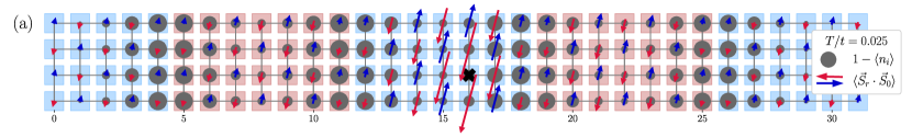
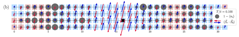
Figure 1: Hole-densities and spin correlations of a typical METTS state $\ket{\psi_{i}}$ for $U/t=10$ at hole-doping $p=1/16$ on a $32\times 4$ cylinder. The diameter of black circles is proportional to the hole-density $1-\braket{n_{l}}=1-\braket{\psi_{i}}{n_{l}}{\psi_{i}}$, the length of the red/blue arrows is proportional to the amplitude of the spin correlation $\braket{\vec{S}_{0}\cdot\vec{S}_{l}}=\braket{\psi_{i}}{\vec{S}_{0}\cdot\vec{S}_{l}}{\psi_{i}}$. The black cross indicates the reference site of the spin correlation. Red/blue squares indicate the sign of the staggered spin correlation $(-1)^{x+y}\braket{\vec{S}_{0}\cdot\vec{S}_{l}}$ (a) $T/t=0.025$. We observe antiferromagnetic domain walls of size $\sim 6-8$ bounded by maxima in the hole-density. This indicates a fluctuating stripe phase realized. (b) $T/t=0.100$. We observe extended antiferromagnetic domains. No regular stripe patterns are formed.

Cluster extensions of dynamical mean-field theory (DMFT) Georges et al. (1996); Maier et al. (2005); Kotliar et al. (2006); Tremblay et al. (2006) on the other hand, address the problem from a different perspective. These methods use the degree of spatial locality as a control parameter and, starting from the high-temperature limit in which the physics is highly local, follow the gradual emergence of non-local physics as spatial correlations grow upon reducing temperature. These methods have established the occurrence of a pseudogap (PG) upon cooling Huscroft et al. (2001); Civelli et al. (2005); Sadovskii et al. (2005); Stanescu and Kotliar (2006); Haule and Kotliar (2007); Zhang and Imada (2007); Imada et al. (2013); Liebsch and Tong (2009); Ferrero et al. (2009, 2009); Gull et al. (2010, 2013); Sordi et al. (2012); Reymbaut et al. (2019) and related this phenomenon to the development of short-range antiferromagnetic correlations Preuss et al. (1997); Macridin et al. (2006); Kyung et al. (2006); Gunnarsson et al. (2015); Wu et al. (2017); Scheurer et al. (2018); Wu et al. (2018). This picture is supported by unbiased quantum Monte Carlo methods without any fermion sign approximations, although these are limited to relatively high temperature Rossi (2017); Gukelberger et al. (2017); Wu et al. (2017); Vučičevic and Ferrero (2020).

These two ways of looking at the problem (ground-state $T=0$ versus finite-$T$ starting from high-$T$), leave the intermediate-$T$ regime as uncharted territory and, crucially, leave a major question unanswered: how does the emergence of the PG at high temperature eventually evolve into the charge inhomogeneous ground states revealed by DMRG and other recent studies?

In this article, we bridge this gap and answer this question for the weakly doped Hubbard model at strong coupling, on a specific lattice geometry. We consider long cylinders of width $4$ and length up to $32$ sites: this is close to the current limit of ground-state DMRG studies, such as the extensive study recently presented in Ref. Jiang et al. (2020). To study this challenging system at finite temperature, we have refined and further developed the minimally entangled typical thermal state (METTS) method White (2009); Stoudenmire and White (2010). This allows us to follow the full evolution of the system as the temperature is increased from the ground state exhibiting stripes. We monitor this evolution through the calculation of several observables, such as the spin and charge structure factors, the momentum distribution function, as well as thermodynamic observables. We determine the onset temperature of the ground state stripe phase. We find that as the system is heated above this onset temperature, a new phase with short-range antiferromagnetic correlations is found, which shares many features with the experimentally observed pseudogap phase. In contrast to the incommensurate correlations observed in the stripe phase, the magnetic correlations are commensurate in this regime. We identify the pseudogap onset temperature, which is distinctly higher than the temperature at which the stripes form.

Finite-temperature simulations using DMRG or tensor network techniques beyond ground-state physics were developed early on, but seemed practical mostly for one dimensional systems. The purification method Verstraete et al. (2004); Feiguin and White (2005) is particularly attractive for its simplicity Tiegel et al. (2014); Becker et al. (2017); Buser et al. (2019), but in the limit of low temperatures, its representation of the mixed state carries twice the entanglement entropy of the ground state, making it unsuitable for wide ladders, although techniques have been developed to reduce the entanglement growth Hauschild et al. (2018). The METTS method White (2009); Stoudenmire and White (2010) was developed to overcome this obstacle. To simulate finite temperatures several matrix product states (MPS) are randomly sampled in a specified way. The computation of a single such MPS (also called a METTS), which has entanglement entropy similar to or less than the ground state, can be performed with the same computational scaling with system size as ground-state DMRG White (2009); Stoudenmire and White (2010); Bruognolo et al. (2017). However, the METTS algorithm requires imaginary time evolution rather than DMRG’s more efficient sweeping to find the ground state, and also a certain amount of random sampling, both of which increase the calculation time significantly. It has been argued that for certain one-dimensional systems, where entropy scaling is less important than sampling error, the METTS algorithm does not outperform the purification approach Binder and Barthel (2015). In this manuscript, we develop and refine the METTS methodology and demonstrate that it can be successfully applied to study the finite temperature properties of the doped Hubbard model in the strong coupling limit on a width-$4$ cylinder.

The manuscript is organised in two major parts. In sections II, III, IV, V and VI we discuss our physical results. We define the model, establish basic notations, and give a minimal explanation of the METTS method in section II. The METTS method allows investigating typical states at a given temperature, which we show in section III. Results on charge and magnetic ordering are then presented in section IV. We discuss the nature of the spin and charge gaps in section V and present results on the specific heat and magnetic susceptibility in section VI. In the second part in sections VII, VIII, IX, X and XI we explain and demonstrate the more technical aspects of our simulations. We explain the details of the algorithms we employ for our simulations in section VII. We discuss the accuracy of the imaginary-time evolution algorithms we employ in section VIII and investigate the METTS entanglement section IX. We demonstrate that we can achieve agreement with different numerical methods within their respective limits in sections X and XI. Finally, we discuss the physical implications of our results and the perspectives opened by our work in sections XII and XIII. The statistical properties of the METTS time series are discussed in appendix A. There, we give the reason why these simulations can actually be performed at a reasonable computational cost. We demonstrate that the the variance of several estimators quickly decreases when lowering temperatures as well as increasing system sizes.

II Model and Method

We consider the single-band Hubbard model on the square lattice,

$$H=-t\sum_{\langle i,j\rangle,\sigma}\left(c^{\dagger}_{i\sigma}c_{j\sigma}+c^{\dagger}_{j\sigma}c_{i\sigma}\right)+U\sum_{i}n_{i\uparrow}n_{i\downarrow},$$ (1)

where $\sigma=\uparrow,\downarrow$ denotes the fermion spin, $c^{\dagger}_{i\sigma}$ and $c_{i\sigma}$ denote the fermionic creation and annihilation operators, and $n_{i\sigma}=c^{\dagger}_{i\sigma}c_{i\sigma}$ denotes the fermion number operator. The system is studied on a cylinder with open boundary conditions in the long direction and periodic boundary conditions in the short direction. We denote the length of the cylinder $L$, the width $W$, with the number of sites $N=L\times W$. The cylindrical geometry is adopted since our computations are performed using MPS techniques. When studying the system using METTS, we employ the canonical ensemble with fixed particle number $N_{\textrm{p}}$. Thermal expectation values of an observable $\mathcal{O}$ are given by,

$$\braket{\mathcal{O}}=\frac{1}{\mathcal{Z}}\operatorname{Tr}(\text{e}^{-\beta H}\mathcal{O}).$$ (2)

Here, $\beta=1/k_{\mathrm{B}}T$ denotes the inverse temperature and $\mathcal{Z}=\operatorname{Tr}(\text{e}^{-\beta H})$ denotes the partition function. We henceforth set $k_{\mathrm{B}}=1$. Results are presented depending on the hole-doping,

$$p=1-n,$$ (3)

where $n=N_{\textrm{p}}/N$ denotes the particle number density.

We study the finite-temperature properties of the Hubbard model Eq. 1 on a $L=32$ and $W=4$ square cylinder in the strong-coupling regime at $U/t=10$ and focus on the hole-doped case $p=1/16$. We also performed simulations at half-filling for comparison. Simulations have been performed for a temperature range,

$$T/t=0.0125,\;0.0250,\;\ldots\;,0.5000.$$ (4)

To evaluate thermal expectation values, the METTS algorithm averages over expectation values of pure states $\ket{\psi_{i}}$,

$$\braket{\mathcal{O}}=\overline{\braket{\psi_{i}}{\mathcal{O}}{\psi_{i}}}.$$ (5)

Here, $\overline{\cdots}$ denotes averaging over random realizations of $\ket{\psi_{i}}$, which are called minimally-entangled typical thermal states (METTS). We discuss the METTS algorithm in detail in section VII.1. While in principle, the basic METTS algorithm is unbiased and exact, the computation of the states $\ket{\psi_{i}}$ amounts to an imaginary-time evolution of product states, which is performed using tensor network techniques. As shown in section VIII, this operation can be performed to a high precision using modern MPS time-evolution algorithms. The accuracy is controlled by the maximal bond dimension $D_{\max}$ of the MPS representation of each METTS $\ket{\psi_{i}}$ and by the number of METTS sampled. Our implementation is based on the ITensor library Fishman et al. (2020).

III METTS snapshots at finite temperature

The METTS $\ket{\psi_{i}}$ can be considered “snapshots” of the thermal state at a given temperature. It is, therefore, informative to study properties of individual METTS. The METTS naturally separate the fluctuations of the system into mostly-quantum and mostly-thermal. The mostly-quantum, higher-energy fluctuations are contained within individual METTS, while long-distance low-energy fluctuations tend to appear via the sampling over different METTS. At zero temperature, all METTS are identically the ground state. At infinite temperature, they are classical product states with each site randomly in one of the four basis states of a single site. We illustrate some typical METTS on the $32\times 4$ square cylinder at $U/t=10$ and $p=1/16$ in Fig. 1. Hole-densities at site $l$, $1-\braket{\psi_{i}}{n_{l}}{\psi_{i}}$, where $n_{l}=n_{l\uparrow}+n_{l\downarrow}$, are shown as black circles. Spin correlations, $\braket{\psi_{i}}{\vec{S}_{l}\cdot\vec{S}_{m}}{\psi_{i}}$, are shown as red and blue arrows. We choose a reference site $l=0$, indicated by the black cross in the middle of the lattice. For states at temperature $T/t=0.025$, like the state shown in Fig. 1(a), we observe regular charge density wave patterns with a wavelength of $6\sim 8$ lattice sites. This charge modulation is accompanied by the staggered spin correlations changing their sign, as indicated by the blue and red squares. We, thus, observe antiferromagnetic domains of the size of the charge wavelength. The number of observed charge stripes on the $32\times 4$ cylinder is $4$. Since hole-doping $p=1/16$ corresponds to $8$ holes on this lattice, we have two holes per stripe and thus observe a half-filled stripe on the width $4$ cylinder. We show a typical METTS state at temperature $T/t=0.100$ in Fig. 1(b). At this temperature, we do not find regular charge density wave patterns. However, we observe enhanced antiferromagnetic correlations with larger antiferromagnetic domains.

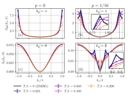
Figure 2: Magnetic and charge structure factors, $S_{\textrm{m}}(\bm{k})$ and $S_{\textrm{c}}(\bm{k})$, of the $32\times 4$ square cylinder at $U/t=10$ for $p=0$ (left) and $p=1/16$ (right). We compare different temperatures from METTS with $D_{\max}=2000$ and ground-state DMRG with $D_{\max}=5000$. (a) Magnetic structure factor for $p=0$ and $k_{y}=\pi$. The peak at $\bm{k}=(\pi,\pi)$ indicates the antiferromagnetism. (b) Magnetic structure factor for $p=1/16$ and $k_{y}=\pi$. The peak at $\bm{k}=(7\pi/8,\pi)$ (gray dashed line) indicates the stripe order illustrated in Fig. 1(a). (c) Charge structure factor for $p=0$ and $k_{y}=0$. The quadratic behavior at $k_{x}=0$ indicates a gap to charged excitations. (d) Charge structure factor for $p=1/16$ and $k_{y}=0$. We observe a peak at $\bm{k}=(\pi/4,0)$ (gray dotted line). This indicates a half-filled stripe phase at low temperatures. The approximately linear behavior at $k_{x}=0$ indicates a small or vanishing charge gap. In all cases we find the METTS results converging towards the DMRG results in the limit $T\rightarrow 0$.

IV Magnetic and Charge ordering

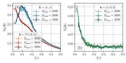
Figure 3: Magnetic and charge structure factors at the ordering vectors of the $32\times 4$ square cylinder at $U/t=10$ for $p=1/16$. We compare results from METTS with $D_{\max}=2000,3000,4000$. (a) Magnetic structure factor $S_{\textrm{m}}(\bm{k})$. The antiferromagnetic ordering vector $\bm{k}=(\pi,\pi)$ is shown in blue. The ordering vector of the half-filled stripes $\bm{k}=(7\pi/8,\pi)$ is shown in red. (b) Charge structure factor $S_{\textrm{c}}(\bm{k})$ at stripe ordering vector $\bm{k}=(\pi/4,0)$. A transition from stripe-order to short-range antiferromagnetic order takes place at $T/t\approx 0.05$. We find agreement between simulations at different bond dimensions.

To quantify these observations, we investigate the magnetic structure factor,

$$S_{\textrm{m}}(\bm{k})=\frac{1}{N}\sum_{l,m=1}^{N}\text{e}^{i\bm{k}\cdot(\bm{r}_{l}-\bm{r}_{m})}\braket{\vec{S}_{l}\cdot\vec{S}_{m}}.$$ (6)

Here, $\bm{r}_{l}$ denotes the coordinate of the $l$-th lattice point, and $\bm{k}=(k_{x},k_{y})$ denotes the quasi-momentum in reciprocal space. The width $W=4$ cylinders we focus on, resolve four momenta in the $y$-direction,

$$k_{y}=0,\pm\pi/2,\pi.$$ (7)

Furthermore, we investigate the charge structure factor,

$$S_{\textrm{c}}(\bm{k})=\frac{1}{N}\sum_{l,m=1}^{N}\text{e}^{i\bm{k}\cdot(\bm{r}_{l}-\bm{r}_{m})}\braket{(n_{l}-n)(n_{m}-n)}.$$ (8)

We show the magnetic structure factors with $y$-momentum $k_{y}=\pi$ for $p=0$ and $p=1/16$ for several select temperatures in Fig. 2(a,b). The METTS simulations shown here have been performed with $D_{\max}=2000$. The convergence of these results as a function of bond dimension for specific values of $\bm{k}$ is shown in Fig. 3. Ground-state DMRG calculations have been performed to obtain results for $T=0$, shown as the gray line. The DMRG results have been performed using $30$ sweeps at maximal bond dimensions up to $D_{\max}=5000$. We observe convergence in the displayed quantities. At half-filling, $p=0$, in Fig. 2(a) we observe a prominent peak at wave vector $\bm{k}=(\pi,\pi)$, which corresponds to the antiferromagnetic ordering vector. We observe convergence of the structure factor at temperatures $T/t=0.050,0.025$ for $T\rightarrow 0$ towards the DMRG results.

At hole-doping $p=1/16$ in Fig. 2(b) we observe that at temperatures below $T/t\approx 0.050$ the peak in the magnetic structure factor is shifted by $\delta=\pi/8$ away from $\bm{k}=(\pi,\pi)$ towards $\bm{k}=(7\pi/8,\pi)$. This feature is a signature of the formation of stripes, where the shift in the antiferromagnetic ordering vector is induced by the antiferromagnetic domains of opposite polarization, as observed in Fig. 1(a). The accompanying charge modulation is quantified by the charge structure factor shown in Fig. 2(d). We observe a peak at wave vector $\bm{k}=(\pi/4,0)=(2\delta,0)$. Hence, the charge modulations occur at half the wavelength of the antiferromagnetic modulations. We again find that the METTS results tend towards the $T=0$ DMRG results as $T\rightarrow 0$.

Above $T/t\approx 0.050$, we notice that the peak in the magnetic structure factor is shifted back towards the antiferromagnetic ordering vector $\bm{k}=(\pi,\pi)$, as shown for $T/t=0.100$. We show the temperature dependence of the magnetic structure factor for both ordering vectors in Fig. 3(a). We find that above $T/t\approx 0.050$, $\bm{k}=(\pi,\pi)$ is the dominant ordering vector with a maximum in the structure factor attained at $T/t\approx 0.100$. Below $T/t\approx 0.050$, the stripe ordering vector $\bm{k}=(7\pi/8,\pi)$ is dominant. This suggests a transition or crossover from the stripe phase, to a new phase with antiferromagnetic correlations. The realization of the stripe phase at low temperatures is also apparent in the behavior of the charge structure factor at ordering vector $\bm{k}=(\pi/4,0)$ in Fig. 3(b). We observe a sharp increase below, $T/t\approx 0.050$. We also compare the structure factors from METTS simulations at different bond dimensions $D_{\max}$ in Fig. 3 and observe agreement within errorbars for most parameters. The peak height of the magnetic structure factor at $\bm{k}=(\pi,\pi)$ is slightly decreased for $D_{\max}=2000$.

V Gaps and correlations in the doped system

We now focus on the charge and spin excitations in the hole-doped case, $p=1/16$. Generally, the behavior of a particular type of correlation function is tied to the presence or absence of an associated gap. Consider the density structure factor in the vicinity of $\bm{k}=(0,0)$ in Fig. 2(c,d). Its behavior differs significantly between the half-filled case in Fig. 2(c) and the $p=1/16$ hole-doped case in Fig. 2(d). We observe that for $p=0$,

$$S_{\textrm{c}}(k_{x},0)\approx\textrm{const }k_{x}^{2}.$$ (9)

This behavior is expected for a system with a charge gap Feynman (1954); Capello et al. (2005); Tocchio et al. (2011); De Franco et al. (2018); Szasz et al. (2020). The charge gap in question is defined (at $T=0$) as

$$\begin{split}\Delta_{\textrm{c}}^{(2)}=&\frac{1}{2}[E_{0}(m+1,m+1)+E_{0}(m-1,m-1)\\ &-2E_{0}(m,m)],\end{split}$$ (10)

where $E_{0}(N_{\uparrow},N_{\downarrow})$ is the ground state energy with $N_{\uparrow}$ and $N_{\downarrow}$ up and down particles. A charge gap, in the thermodynamic limit, implies that the system favors that particular doping compared to states differing by two particles. Typically, this only happens at commensurate fillings (such as half-filling) where the filling is a small-denominator simple fraction. We do not expect a doping of $p=1/16$ to have a charge gap. For charge-gapless systems, the behavior of the charge structure factor close to $\bm{k}=(0,0)$ is expected to be Capello et al. (2005); Tocchio et al. (2011); De Franco et al. (2018),

$$S_{\textrm{c}}(k_{x},0)\approx\textrm{const }|k_{x}|.$$ (11)

We observe this behavior for hole-doping $p=1/16$ in Fig. 2(d), consistent with the absence of a charge gap.

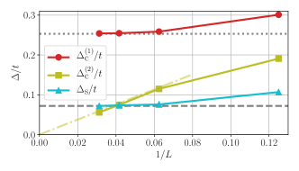
Figure 4: Gaps for $U/t=10$ at hole-doping $p=1/16$ on $L\times 4$ cylinders for different cylinder lengths $L$ from DMRG using Eqs. 12, 10 and 13. We find that for large cylinder lengths, the single-particle gap $\Delta_{\textrm{c}}$ and the spin gap $\Delta_{\textrm{s}}$ approach finite values $\Delta_{\textrm{c}}^{(1)}/t\approx 0.25$ and $\Delta_{\textrm{s}}/t\approx 0.07$. The charge gap $\Delta_{\textrm{c}}^{(2)}$ vanishes $\propto 1/L$ despite being of order $0.1$ on the finite size lattices. The dashed and dotted lines are a guide to the eye.

We also define the single particle gap,

$$\Delta_{\textrm{c}}^{(1)}=\frac{1}{2}[E_{0}(m+1,m)+E_{0}(m-1,m)-2E_{0}(m,m)],$$ (12)

and the spin gap,

$$\Delta_{\textrm{s}}=E_{0}(m+1,m-1)-E_{0}(m,m).$$ (13)

In Fig. 4 we show these three types of gaps for $p=1/16$, evaluated using DMRG with fixed particle and spin quantum numbers on cylinders of length $8$, $16$, $24$, and $32$. We checked that the computed gaps correspond to bulk excitations, by investigating the density distribution upon adding and removing particles. This showed that additional particles or holes are indeed inserted in the bulk of the system. The single particle gap $\Delta_{\textrm{c}}^{(1)}$ approaches a finite value $\Delta_{\textrm{c}}^{(1)}/t\approx 0.25$, and the spin gap $\Delta_{\textrm{s}}$ approaches a finite value of $\Delta_{\textrm{s}}/t\approx 0.07$. In contrast, the charge gap decreases approximately as $1/L$ for $L=16,24,32$, consistent with a vanishing charge gap in the $L\to\infty$ limit, in agreement with previous DMRG results on the width 4 cylinder Jiang et al. (2020). Our observations on the stripe phase agree well with the Luther-Emery 1 (LE1) phase in Ref. Jiang et al. (2020). In particular, a finite single particle gap has analogously been reported.

The single particle gap is closely tied to the behavior of the momentum distribution function,

$$n_{\sigma}(\bm{k})=\frac{1}{N}\sum_{l,m=1}^{N}\text{e}^{i\bm{k}\cdot(\bm{r}_{l}-\bm{r}_{m})}\braket{c^{\dagger}_{l\sigma}c_{m\sigma}}$$ (14)

as one varies $\bm{k}$. Of course, our single particle gap computed from Eq. (12) is the minimum gap as one varies the momentum. Gaps at other momenta could be obtained from spectral functions, but these are beyond the scope of this work. However, we can observe very different behavior in $n_{\sigma}(\bm{k})$ for different $\bm{k}$. Results for different $\bm{k}$ and also several temperatures are shown in Fig. 5. For a system with a Fermi surface, the momentum distribution function is expected to be discontinuous at the Fermi momentum Luttinger (1960). Although for DMRG at finite length and bond dimension this discontinuity is usually not directly observed, the slope of the momentum distribution function as a function of bond dimension can be investigated to diagnose a Fermi surface Szasz et al. (2020).

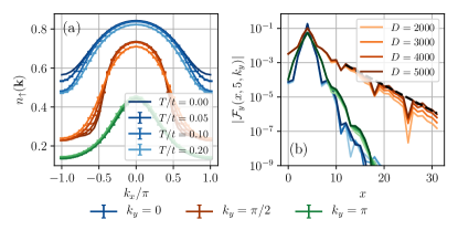
Figure 5: (a) Momentum distribution function $n_{\uparrow}(\bm{k})$ of the $32\times 4$ square cylinder at $U/t=10$ for $p=1/16$. (b) Ground state single-particle correlation function from DMRG after Fourier transform in $y$-direction, $\mathcal{F}_{y}(x_{l},x_{m},k_{y})$. At $k_{y}=\pi/2$ we observe a slow exponential decay, hinting towards a small charge gap at this wave vector.

We find the maximal slope of the momentum distribution function $n_{\sigma}(\bm{k})$ to remain finite for all values of $k_{y}$, consistent with a single particle gap. The steepest slope of $n_{\sigma}(\bm{k})$ is observed at $y$-momentum $k_{y}=\pi/2$. There, we observe that $n_{\sigma}(\bm{k})$ at different temperatures intersect at a specific value close to the nodal point $\bm{k}=(\pi/2,\pi/2)$. We do not observe such an intersection for $k_{y}=0$. The small slope for $k_{y}=0$ and $k_{y}=\pi$ suggests a large single-particle gap at these lines in the Brillouin zone, while the larger slope close to the nodal point suggests a smaller single-particle gap.

A spectral gap implies exponentially decaying ground-state correlation functions in real space Hastings and Koma (2006), where a slow exponential decay is a signature of a small gap. We display the single-particle correlation function at $p=1/16$ from DMRG after Fourier transform in the $y$-direction in Fig. 5(b). The quantity shown is

$$\mathcal{F}_{y}(x_{l},x_{m},k_{y})=\frac{1}{W}\sum_{n,m=1}^{W}\textrm{e}^{ik_{y}(y_{n}-y_{m})}\braket{c^{\dagger}_{(x_{l},y_{n})}c_{(x_{m},y_{m})}},$$ (15)

where $W=4$ denotes the width of the cylinder. Results are shown for $k_{y}=0,\pi/2,\pi$ and as a function of bond dimension. We find the slowest decay is found for $k_{y}=\pi/2$, with fast exponential decay for $k_{y}=0$ and $k_{y}=\pi$. This demonstrates that the gap to charged excitations is smallest at $k_{y}=\pi/2$.

It is interesting to compare the magnitude of the single particle gap and the spin gap, both with each other and with the temperatures associated with the onset of short-range antiferromagnetic order and the onset of stripes. The onset of local antiferromagnetic correlations is associated with the peak in the specific heat and maximum of the uniform susceptibility, discussed in the next section, which is slightly above $0.2t$. This is close in magnitude to the single particle gap, $0.25t$, and so it is tempting to tie them together. One could consider a linkage of these energy scales through pair-binding. A simple picture of pair binding is that two holes together disrupt the local antiferromagnetic correlations less than two separate holes. This mechanism could only occur below the onset temperature of local antiferromagnetism.

It is also tempting to tie the spin gap (about $0.07t$) to the onset temperature of stripes, $0.05t$. However, this linkage is not so clear. The spin gap is probably strongly influenced by the finite width of the cylinder. At half-filling, in the Heisenberg limit, even-width cylinders have a spin gap which vanishes exponentially with the width, and the 2D limit is gapless. It is also not clear that a striped state should have a spin gap, so the similarity in the spin-gap and stripe energy scales for the $N_{y}=4$ system may be a coincidence.

VI Thermodynamics

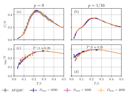
Figure 6: Specific heat $C$ and magnetic susceptibility $\chi_{\textrm{m}}$ at $U/t=10$ of a $32\times 4$ square cylinder for hole-dopings $p=0$ (left) and $p=1/16$ (right). We compare results METTS using different maximal bond dimensions $D_{\max}=2000,3000,4000$. (a) Specific heat, $p=0$. Results from all maximal bond dimensions agree. We find a $C\propto T^{2}$ behavior at low temperature, predicted from spin-wave theory of an antiferromagnet. We also show exact AFQMC data on the same system, which agrees within errorbars (b) Specific heat, $p=1/16$. We observe a step-like feature around $T/t=0.05$, where we locate the transition to the stripe phase in Fig. 2. In the range $T/t\approx 0.075$ to $T/t\approx 0.175$ we observe an approximately linear behavior. (c) Magnetic susceptibility at $p=0$. We observe a maximum at $T^{\times}/t\approx 0.29$. (d) Magnetic susceptibility at $p=1/16$. A maximum is located at $T^{*}/t\approx 0.25$.

Finally, we discuss basic thermodynamics quantities for half-filling and $p=1/16$. The specific heat is given by,

$$C=\frac{\textrm{d}E}{\textrm{d}T}=\beta^{2}\;\left[\braket{H^{2}}-\braket{H}^{2}\right].$$ (16)

When using the METTS algorithm, we compute the numerical derivative of measurements of the total energy $E=\braket{H}$. We perform a total-variation regularization of the differentiation as explained in appendix B. We find this approach advantageous to evaluating the fluctuation of energy as in the second expression of Eq. 16. We observe that evaluating the energy fluctuation requires larger MPS bond dimensions to achieve convergence. The magnetic susceptibility is given by

$$\chi_{\textrm{m}}=\left.\frac{\textrm{d}M}{\textrm{d}H}\right|_{H=0}=\beta\left[\braket{(S^{z}_{\textrm{tot}})^{2}}-\braket{S^{z}_{\textrm{tot}}}^{2}\right],$$ (17)

where $M=\langle S^{z}_{\textrm{tot}}\rangle$ denotes the total magnetization, and $H$ an applied magnetic field. In contrast to the specific heat, we find that the fluctuation in the second expression of Eq. 17 can be evaluated efficiently.

Results for the specific heat and magnetic susceptibility at half filling and $p=1/16$ are shown in Fig. 6. At half filling, shown in Fig. 6(a) we find that the specific heat is well converged at $D_{\max}=2000$. At low temperature, we observe a behavior $C\propto T^{2}$, which is expected for an antiferromagnetic insulator from spin-wave theory Kubo (1952); Dyson (1956); Yamamoto and Noriki (2019). The thermodynamics at half filling closely resembles the thermodynamics of the square lattice Heisenberg model Miyashita (1988); Gomez-Santos et al. (1989); Okabe and Kikuchi (1988); Manousakis (1991). Previous quantum Monte Carlo studies Miyashita (1988); Gomez-Santos et al. (1989); Okabe and Kikuchi (1988) have shown that the two-dimensional antiferromagnetic square lattice exhibits a maximum in the specific heat at $T/J\approx 0.5$. The energy scale exchange interaction in the Hubbard model is given by $J=4t^{2}/U$, which for $t=1$ and $U=10$ evaluates to $J=0.4$. Hence, the observed maximum in the specific heat at $T/t\approx 0.2=J/2$ agrees well with the Heisenberg case. The magnetic susceptibility at half-filling shown in Fig. 6(c) is also converged at a bond dimension $D_{\max}=2000$. It exhibits a maximum at $T^{\times}/t\approx 0.29$, which indicates the onset of antiferromagnetic correlations. In the Heisenberg antiferromagnet, the magnetic susceptibility exhibits a maximum at $T/J\approx 1.0$. We find, that in our case this maximum is shifted to slightly lower temperatures, as can analogously be observed in previous quantum Monte Carlo results of the Heisenberg model on finite width ladders Frischmuth et al. (1996).

Turning to the thermodynamics at hole doping $p=1/16$ we also find the specific heat Fig. 6(b) to be well converged at $D_{\max}=2000$. It exhibits a broad maximum around $T/t\approx 0.2$, at a similar temperature as the half-filled case. But at temperatures around $T/t\approx 0.07$ we also observe a small step-like feature. This temperature corresponds well with the onset temperature of stripe order from Fig. 3 as well as the spin gap shown in Fig. 4. Between the step-like feature and the maximum from $T/t\approx 0.08$ to $T/t\approx 0.175$ we observe a regime where the specific heat is approximately linear in temperature, $C\propto T$. Also, below the step-like feature at $T/t=0.07$ our data suggests a linear temperature regime, although this observation is only based on few data points. The magnetic susceptibility in Fig. 6(d) is well converged at $D_{\max}=3000$, where we observe a slight uptick at $D_{\max}=2000$ at lower temperatures. The magnetic susceptibility attains a maximum at $T^{*}/t\approx 0.25$. This compares well to previous results from the finite-temperature Lanczos method Bonča and Prelovšek (2003) on small lattice sizes, that also detected a maximum in the magnetic susceptibility at a comparable temperature and doping. It is also in agreement with calculations of the uniform susceptibility with cluster extensions of DMFT  Haule and Kotliar (2007); Chen et al. (2017). In underdoped cuprate superconductors, the pseudogap was indeed first identified experimentally as a suppression of the magnetic susceptibility below a temperature $T^{*}$ larger than the superconducting $T_{c}$ Alloul et al. (1989); Johnston (1989).

VII METTS simulations of the two-dimensional Hubbard model

In this second part, we demonstrate that the METTS method can indeed be successfully performed for the Hubbard model approaching two-dimensional geometries. We show that several quantities of interest, like specific heat, magnetic susceptibility, structure factors, and momentum distribution functions can be reliably computed with reasonable computational effort over a wide range of temperatures. We discover several interesting facts about the METTS algorithm. A key practical question is how many METTS have to be random sampled. This depends on the variance of the estimator, where a small variance implies that less METTS are needed to achieve a certain statistical error. Interestingly, we find for several quantities, that both decreasing temperature as well as increasing the system size decreases the variance significantly. The METTS algorithm involves computing an imaginary-time evolution of product states. Modern MPS algorithms allow for performing this time evolution with high accuracy. Our mapping of the linear MPS chain onto the two-dimensional square cylinder geometry is shown in Fig. 8. We employ a combination of the time-dependent variational principle (TDVP) Haegeman et al. (2011, 2016), and the time-evolving block decimation (TEBD) Vidal (2003, 2004) algorithms and demonstrate the accuracy of this approach by comparing to numerically exact Lanczos time evolution on a smaller system size. The algorithms we choose, come with several control parameters. We find some of them can be chosen highly accurate without impacting performance or, otherwise, allow for an optimal choice. We identify the maximal bond dimension for performing the TDVP algorithm to be the main control parameter for the accuracy of the imaginary time evolution.

We assess the accuracy by comparing results to two other state-of-the-art methods. Firstly, we compare to the method of thermal pure quantum (TPQ) states Sugiura and Shimizu (2012, 2013); Wietek et al. (2019), which allows simulating smaller systems in a statistically exact way, also at finite-doping. Secondly, we compare to auxiliary-field quantum Monte Carlo (AFQMC). At half-filling, this method is also statistically exact and allows for simulating larger system sizes. Away from half-filling the method cannot be applied without encountering a sign problem, although they can be performed using the constrained-path approximation He et al. (2019). At finite-doping we study our results as a function of the maximal bond dimension and find that several quantities can be converged. The bond dimensions required to do so, are significantly smaller than the bond dimensions reported to converge ground state DMRG calculations.

We focus on the technical and algorithmic aspects of these simulations. The METTS algorithm White (2009); Stoudenmire and White (2010); Bruognolo et al. (2017) combines the advantages of Monte Carlo simulation and tensor network algorithms to simulate finite-temperature quantum many-body systems.

VII.1 Basic METTS algorithm

Figure 7: Illustration of the METTS algorithm. Red arrows indicate imaginary-time evolution of product states $\ket{\sigma_{i}}$ into METTS $\ket{\psi_{i}}$. Green arrows indicate the collapse step, blue arrows indicate performing measurements of observables. This yields a time series of measurements $\braket{\psi_{i}}{\mathcal{O}}{\psi_{i}}$, indicated by gray arrows.

We briefly review the basic steps of the METTS algorithm. For more details we refer to Refs. White (2009); Stoudenmire and White (2010); Bruognolo et al. (2017). Given an orthonormal basis $\{\ket{\sigma_{i}}\}$ of the Hilbert space, the thermal average in Eq. 2 can be written as,

$$\langle\mathcal{O}\rangle =\frac{1}{\mathcal{Z}}\sum_{i}\braket{\sigma_{i}}{\text{e}^{-\beta H/2}\mathcal{O}\text{e}^{-\beta H/2}}{\sigma_{i}}$$ (18)

$$=\frac{1}{\mathcal{Z}}\sum_{i}p_{i}\braket{\psi_{i}}{\mathcal{O}}{\psi_{i}},$$ (19)

where we introduce,

$$p_{i}=\braket{\sigma_{i}}{\text{e}^{-\beta H}}{\sigma_{i}},\;\text{ and }\;\ket{\psi_{i}}=\frac{1}{\sqrt{p_{i}}}\text{e}^{-\beta H/2}\ket{\sigma_{i}}.$$ (20)

The so-called typical thermal states $\ket{\psi_{i}}$ are normalized ($\braket{\psi_{i}}{\psi_{i}}=1$) and the weight $p_{i}$ defines a probability distribution, i.e.

$$p_{i}\geq 0,\quad\frac{1}{\mathcal{Z}}\sum_{i}p_{i}=1.$$ (21)

The thermal average as defined in Eq. 19 is, thus, amenable to Monte Carlo sampling. Notice, that all weights $p_{i}$ are manifestly real and non-negative. Therefore one does not encounter a sign problem when using such an ensemble. The tradeoff is that the states $\ket{\psi_{i}}$ are entangled and one must find a way to represent and manipulate them efficiently.

To construct a Markov chain with stationary distribution $p_{i}$, Refs. White (2009); Stoudenmire and White (2010) introduced the transition probability,

$$T_{i\rightarrow j}=|\braket{\psi_{i}}{\sigma_{j}}|^{2},$$ (22)

which fulfills the detailed balance equations,

$$p_{i}T_{i\rightarrow j}=p_{j}T_{j\rightarrow i}.$$ (23)

According to Markov chain theory, the average of the sequence of measurements,

$$\mathcal{O}_{i}=\braket{\psi_{i}}{\mathcal{O}}{\psi_{i}},\quad i=1,\ldots,R,$$ (24)

converges to the thermal expectation value, i.e.

$$\lim\limits_{R\rightarrow\infty}\frac{1}{R}\sum_{i=1}^{R}\mathcal{O}_{i}=\braket{\mathcal{O}},$$ (25)

almost surely, provided ergodicity. $R$ denotes the length of the measurement sequence, i.e., the number of METTS computed.

The algorithm as described above does not make any reference to tensor networks yet. However, its individual steps can be efficiently performed within the framework of matrix product states (MPS), if the basis states $\ket{\sigma_{i}}$ are only weakly entangled. We take the $\ket{\sigma_{i}}$ to be product states of the form

$$\ket{\sigma_{i}}=\ket{\sigma_{i}^{1}}\ket{\sigma_{i}^{2}}\ldots\ket{\sigma_{i}^{N}},$$ (26)

which are states with zero entanglement. With this choice, the typical thermal states $\ket{\psi_{i}}$ are in a certain sense minimally entangled, hence referred to as METTS.

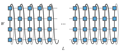
Figure 8: Square cylinder geometry. We consider open boundary conditions in the long direction of length $L$ and periodic boundary conditions in the short direction of width $W$. The black line shows the ordering of the sites when mapping to a matrix-product state. In this manuscript, we focus on the case $W=4$.

We illustrate the METTS algorithm in Fig. 7. It consists of the following basic steps:

1. Initial state: Choose a suitable first state of the Markov chain $\ket{\sigma_{1}}$, set $i\leftarrow 1$.

2. Time evolution: evolve the state $\ket{\sigma_{i}}$ in imaginary time by an amount $\beta/2$ and normalize to compute the state

   $$\ket{\psi_{i}}=\frac{1}{\sqrt{p_{i}}}\text{e}^{-\beta H/2}\ket{\sigma_{i}}.$$ (27)

3. Measurement: measure an observable $\braket{\psi_{i}}{\mathcal{O}}{\psi_{i}}$.

4. Collapse: choose a new basis state $\ket{\sigma_{i+1}}$ according to the probability distribution $|\braket{\psi_{i}}{\sigma_{i+1}}|^{2}$. Set $i\leftarrow i+1$ and iterate from step (ii).

The sequence of measurements $\{\braket{\psi_{i}}{\mathcal{O}}{\psi_{i}}\}$ is then analysed using standard time-series analysis techniques to compute an (error) estimate for the thermal average $\braket{\mathcal{O}}=\frac{1}{R}\sum_{i=1}^{R}\braket{\psi_{i}}{\mathcal{O}}{\psi_{i}}$.

VII.2 Initial State

The choice of the initial product state in the METTS algorithm is rather important and can result in numerical difficulties if improperly chosen. We begin with a random product state. It is chosen according to a uniform distribution on the space of product configurations with a given particle number. Such a state is in general not related to the low-energy physics of the system. Directly starting the METTS procedure from this state can result in long thermalization times, especially at higher temperatures. Also, such unphysical random states can result in large bond dimensions if time evolved with given accuracy and can, therefore, complicate computations. To circumvent this problem, we perform several initial DMRG sweeps on the uniform random initial state to obtain a more physical state. This state is then collapsed to a new product state $|\sigma_{1}\rangle$, which will then be taken as the initial state of the METTS algorithm. These initial DMRG sweeps are not performed until convergence. We typically choose to do $5$ sweeps at maximum bond dimension $D=100$. We also add a noise term White (2005) of $10^{-4}$, which further randomizes the starting state.

VII.3 Imaginary-time evolution

The computation of the imaginary-time evolution,

$$\ket{\psi_{i}}=\text{e}^{-\beta H/2}\ket{\sigma_{i}},$$ (28)

poses the key algorithmic challenge in the METTS algorithm. Time evolution algorithms for matrix product states are subject of current research and several accurate methods have been proposed Vidal (2003, 2004); White and Feiguin (2004); Daley et al. (2004); Haegeman et al. (2011, 2016); Zaletel et al. (2015); Yang and White (2020). The recent review article by Paeckel et al. Paeckel et al. (2019) summarizes and compares a variety of these methods. Among those, the time dependent variational principle (TDVP) Haegeman et al. (2011, 2016) method has been shown to have favorable properties in various scenarios, including imaginary-time evolution.

The TDVP algorithm is closely related to DMRG Haegeman et al. (2016). Instead of solving an effective local eigenvalue problem, a time evolution of the effective Hamiltonian is performed, followed by a backward time evolution on one less site. We refer the reader to Refs. Haegeman et al. (2016); Paeckel et al. (2019) for a detailed description of the algorithm. Similar to DMRG, it comes in a two-site variant and a single-site variant. The two-site variant allows for increasing the bond dimension of the MPS gradually when evolving further in time. The single-site algorithm, on the other hand, keeps the MPS bond dimension fixed. The scaling computational resources of both algorithms is

$$O(ND^{3}d\beta),\quad \textrm{(single-site TDVP)},$$ (29)

$$O(ND^{3}d^{2}\beta),\quad \textrm{(two-site TDVP)},$$ (30)

where $N$ denotes the number of sites, $D$ the MPS bond dimension, and $d$ the site-local dimension. In the case of the Hubbard model, $d=4$. We, therefore, expect the single-site TDVP algorithm to be approximately four times faster than the two-site variant, given a fixed maximal bond dimension $D_{\max}$. We choose a time evolution strategy, where we first increase the MPS bond dimension using two-site TDVP up to a maximal bond dimension $D_{\max}$. Afterward, we switch to a single-site TDVP algorithm at fixed bond dimension $D_{\max}$ for speed. Our implementation is based on the ITensor library and is available online Yang and Fishman (2020).

There is, however, a caveat to directly applying the two-site TDVP algorithm in the context of METTS. TDVP suffers from a projection error onto the manifold of MPS at given bond dimension Haegeman et al. (2011, 2016); Paeckel et al. (2019). This error becomes non-negligible for MPS of small bond dimension. In particular, time evolution of product states as in Eq. 26 will suffer from a substantial projection error.

We circumvent this problem by starting the time evolution with a different method, the time-evolving block decimation (TEBD) Vidal (2003, 2004) algorithm. This method has been widely used in a variety of numerical studies, including applications in the context of METTS White (2009); Stoudenmire and White (2010); Bruognolo et al. (2017). The TEBD algorithm we apply uses a second-order Suzuki-Trotter decomposition,

$$\text{e}^{-\tau H}=\text{e}^{-\tau/2h_{1}}\text{e}^{-\tau/2h_{2}}\cdots\text{e}^{-\tau/2h_{2}}\text{e}^{-\tau/2h_{1}}+O(\tau^{3}),$$ (31)

where $H=\sum\limits_{k}h_{k}$ denotes a decomposition of the Hamiltonian into local interaction terms. When interaction terms connect sites that are not adjacent in the MPS ordering, swap gates are applied Stoudenmire and White (2010). In the two-dimensional cylinder geometry shown in Fig. 8 this is done for all hopping terms in the long direction and hopping terms “wrapping” the cylinder in the short direction. For details on implementing swap gates in for two-dimensional systems, we refer the reader to Ref. Stoudenmire and White (2010).

Figure 9: Sketch of the MPS time evolution strategy and bond dimension $D$ as a function of imaginary-time $\tau$. An initial TEBD upto $\tau_{\textrm{TEBD}}$ is followed by a two-site TDVP evolution. Once the MPS reaches a maximum bond dimension $D_{\max}$, we apply the single-site TDVP algorithm until time $\beta/2$.

We summarize our time evolution strategy in Fig. 9. Initially, we apply the TEBD with high accuracy up to an imaginary time $\tau_{\textrm{TEBD}}$ to obtain an MPS with a suitably large bond dimension. Thereafter, we employ the two-site TDVP algorithm to further increase the bond dimension as we go lower in temperature. The TDVP time evolution can decrease the bond dimension obtained after TEBD at intermediate times since it is usually performed with a lower cutoff $\varepsilon$. Once we encounter maximum bond dimension $D_{\max}$, we switch to single-site TDVP for computational efficiency.

Several parameters control the accuracy of our time evolution strategy. We have performed an extensive investigation of their behavior, which we discuss in section VIII. Summarily we find, that most parameters can be kept at a fixed value. The initial TEBD parameters can be chosen highly accurately to not yield any substantial error. For the TDVP time step $\Delta\tau$ there appears to be an optimal choice. We find that a choice of

$$\Delta\tau=0.02,\enskip\varepsilon=10^{-12},\enskip\tau_{\textrm{TEBD}}=0.1,\quad\text{(TEBD)},$$ (32)

yields a negligible time-evolution, as well as TDVP projection error. The two-site TDVP algorithm comes with two control parameters. The time step size $\Delta\tau$ and the SVD cutoff $\varepsilon$. We analyze the accuracy of the time evolution when varying these two parameters over several orders of magnitude in Fig. 10. We find that the cutoff parameter $\varepsilon$ is directly related to the accuracy. Remarkably, we find that for most choices of the cutoff $\varepsilon$, a time step size of

$$\Delta\tau=0.5\quad\text{(TDVP)},$$ (33)

yields optimal accuracy and is also favorable in terms of computational efficiency. Different studies have analogously reported that TDVP allows for rather large time steps Paeckel et al. (2019); Bauernfeind and Aichhorn (2020). The final control parameter is given by the maximal bond dimension $D_{\max}$ used in the single-site TDVP.

VII.4 Collapse

After performing measurements on the state $\ket{\psi_{i}}$, we choose a new product state $\ket{\sigma_{i+1}}$ in step (iv) of the METTS algorithm. $\ket{\sigma_{i+1}}$ is chosen according to the probability distribution $|\braket{\psi_{i}}{\sigma_{i+1}}|^{2}$. The algorithm we use for sampling a random product state from an MPS is described in detail in Ref. Stoudenmire and White (2010). The computational cost of the collapse step is

$$O(ND^{2}d),\quad\textrm{(collapse)}$$ (34)

where $N$ denotes the number of sites, $D$ the MPS bond dimension, and $d$ the site-local dimension. This is a subleading computational cost as compared to the time-evolution, whose computational cost scales as $O(ND^{3}\beta d)$.

There is a freedom of choice of the product state basis. Here, we consider two bases. The local $S^{z}$-basis is given by the states,

$$\ket{\sigma_{i}^{l}}\in\{\ket{\emptyset},\ket{\uparrow},\ket{\downarrow},\ket{\uparrow\downarrow}\}.$$ (35)

A collapse into this basis will conserve particle number and total magnetization. Since also the imaginary-time evolution conserves all quantum numbers, the METTS will always stay in the same particle number and magnetization sector if the METTS $\ket{\psi_{i}}$ is collapsed into this basis. For simulating the canonical ensemble we have to allow for fluctuations in the magnetization. This can be achieved by projecting into the local $S^{x}$-basis,

$$\ket{\sigma_{i}^{l}}\in\{\ket{\emptyset},\ket{+},\ket{-},\ket{\uparrow\downarrow}\},$$ (36)

where,

$$\ket{+}=\frac{1}{\sqrt{2}}(\ket{\uparrow}+\ket{\downarrow}),\quad\ket{-}=\frac{1}{\sqrt{2}}(\ket{\uparrow}-\ket{\downarrow}).$$ (37)

Since $S^{x}$ and $S^{z}$ do not commute, the magnetization in $S^{x}$ direction can fluctuate for a state with fixed $S^{z}$ magnetization. Since the full Hubbard Hamiltonian is SU($2$) invariant, the state projected into the $S^{x}$ can be rotated into a state in the $S^{z}$ basis. Therefore, we can reinterpret the $S^{x}$ basis as the $S^{z}$ basis with a fixed total magnetization. This allows us to employ $S^{z}$ conservation in the time-evolution algorithm again.

Apart from allowing fluctuations in magnetization, the $S^{x}$ updates yield favorable mixing properties for the Markov chain. We discuss this in detail in appendix A. We find that the collapse into the $S^{x}$-basis not only allows for fluctuation of the magnetization but also reduces autocorrelation effects considerably.

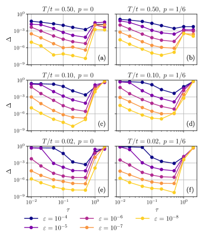
Figure 10: Accuracy of imaginary-time evolution. We compare the overlap defect $\Delta$ for different choices of the TDVP cutoff $\varepsilon$ and time step $\tau$. We investigate temperatures $T/t=0.50$ ($\beta/2=1$) in (a,b), $T/t=0.10$ ($\beta/2=5$) in (c,d), and $T/t=0.02$ ($\beta/2=25$) in (e,f). The left (resp. right) panels show time evolutions of the state $\ket{\sigma_{p=0}}$ (resp. $\ket{\sigma_{p=1/6}}$), where we choose $U/t=10$. The defect is directly related to the cutoff $\varepsilon$. A choice of $\tau=0.5$ is optimal in most circumstances. The accuracy does not appear to deteriorate at lower temperatures.

VIII Time evolution accuracy

Several parameters set the accuracy of the imaginary-time evolution method we describe in section VII.3. We denote the METTS state computed using the MPS techniques by $\ket{\psi^{\textrm{MPS}}}$. In order to assess their accuracy we compute overlaps with METTS states $\ket{\psi^{\textrm{ED}}}$, which have been computed using Exact Diagonalization (ED). We choose a cylindrical system with $L=3$ and $W=4$. Although this lattice is rather small, it already introduces longer-range interactions, that are present in $W=4$ cylinders and, thus, already poses a non-trivial problem for MPS time-evolution techniques. This system is also already too large to easily perform full ED. Therefore, we use a Lanczos method Lanczos (1950); Hochbruck and Lubich (1997) to compute the exact reference state $\ket{\psi^{\textrm{ED}}}$. We apply the algorithm and convergence criterion suggested in Ref. Sidje (1998). We compute the state $\ket{\psi^{\textrm{ED}}}$ up to a precision of $10^{-12}$, in the sense that,

$$1-|\braket{\psi^{\textrm{ED}}}{\psi^{\textrm{exact}}}|^{2}<10^{-12}.$$ (38)

Hence, the state $\ket{\psi^{\textrm{ED}}}$ can be considered as quasi-exact. We choose the defect $\Delta$,

$$\Delta\equiv 1-|\braket{\psi^{\textrm{MPS}}}{\psi^{\textrm{ED}}}|^{2},$$ (39)

as a figure of merit to assess the accuracy of the MPS time evolution. For a given MPS state $\ket{\psi^{\textrm{MPS}}}$ we compute this overlap exactly, by computing the coefficients in the computational basis of the ED code.

We study two different initial product states. We considered the Néel antiferromagnetic state at half-filling, $p=0$, and an antiferromagnetic state, with two holes in the center of the system, $p=1/6$,

$$\ket{\sigma_{p=0}}=\left|\begin{matrix}\uparrow&\downarrow&\uparrow\\ \downarrow&\uparrow&\downarrow\\ \uparrow&\downarrow&\uparrow\\ \downarrow&\uparrow&\downarrow\\ \end{matrix}\right\rangle\quad\text{and}\quad\ket{\sigma_{p=1/6}}=\left|\begin{matrix}\uparrow&\downarrow&\uparrow\\ \downarrow&\emptyset&\downarrow\\ \uparrow&\emptyset&\uparrow\\ \downarrow&\uparrow&\downarrow\\ \end{matrix}\right\rangle.$$ (40)

We focus on METTS $\ket{\psi^{\textrm{MPS}}}$ at temperatures $T/t=0.50,0.10,0.02$ and choose $U/t=10$.

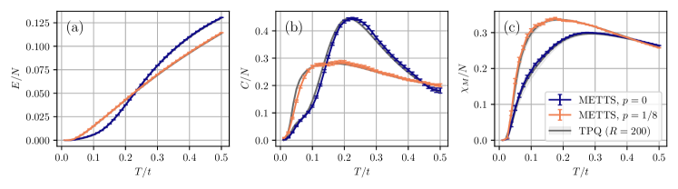
Figure 11: Comparison of thermodynamics from METTS with TPQ on a $4\times 4$ cylinder for hole-dopings $p=0$ and $p=1/8$. For TPQ we used $R=200$ random vectors to obtain the statistical error indicated by the error tubes. (a) Internal energy $E=\braket{H}$ as a function of temperature. (b) Specific heat $C=\text{d}E/\text{d}T$, obtained from numerical differentiation of the energy. We applied a Tikhonov regularization with $\alpha=0.1$ to compute the derivative. (c) magnetic susceptibility $\chi_{\textrm{m}}$. We find agreement within errorbars. We used a cutoff of $\varepsilon=10^{-6}$ and a maximum bond dimension $D_{\max}=2000$ for imaginary-time evolution in METTS.

In order to avoid the projection error of TDVP when directly applied to product states, we start with a precise TEBD time evolution up to time $\beta=0.1$. For doing so, we choose a time-step $\tau_{\textrm{TEBD}}=0.02$ and a cutoff $\varepsilon_{\textrm{TEBD}}=10^{-12}$. These parameters are chosen, such that the time evolved state at $\beta=0.1$ is highly accurate, albeit with a potentially large bond dimension. The large bond dimension, however, is beneficial for decreasing the TDVP projection error Paeckel et al. (2019).

The total defect $\Delta$ in Eq. 39 comprises the error from the initial TEBD evolution, $\Delta_{\text{TEBD}}$, the TDVP projection error, $\Delta_{\text{Proj}}$, and the error of the bulk TDVP evolution, $\Delta_{\text{TDVP}}$. Hence,

$$\Delta\approx\Delta_{\text{TEBD}}+\Delta_{\text{Proj}}+\Delta_{\text{TDVP}}.$$ (41)

As shown in Fig. 10, we achieve total defects smaller than $\Delta<10^{-8}$. The total defect is directly related to the TDVP parameters $\tau$ and $\varepsilon$. Therefore, we conclude that both the initial TEBD evolution error, $\Delta_{\text{TEBD}}$, and the TDVP projection error, $\Delta_{\text{Proj}}$ are negligible as compared to the bulk TDVP evolution error.

We now focus on the two remaining control parameters of the two-site TDVP algorithm. We consider the step-size $\tau$ for one TDVP sweep and the cutoff parameter $\varepsilon$, which is used both as the magnitude of the discarded weight and the accuracy of the local effective time-evolution, cf. section VII.3. Results for the obtained defect $\Delta$ over a broad range of step-sizes and cutoffs are presented in Fig. 10. We observe that for all temperatures and hole-dopings choosing small time steps does not improve the error. In fact, in several cases, a time step of $\Delta\tau=0.01$ yields the largest defect. This behavior is explained by the fact, that smaller time steps require more time steps to be performed. Since at every time step, an additional truncation of the MPS is performed, more time steps accumulate more truncation errors. Interestingly, we find that a choice of $\Delta\tau=0.5$ yields optimal results for most temperatures, cutoffs, and dopings. Larger time steps then again decrease accuracy. Remarkably, we do not observe that the accuracy deteriorates strongly for longer time evolutions of the states we have chosen. The defect is directly related to the cutoff $\varepsilon$. In several cases for $\Delta\tau=0.2$ and $\Delta\tau=0.5$ we find, that the defect is of the same order of magnitude as $\varepsilon$.

These observations let us conclude, that a $\Delta\tau=0.5$ for TDVP is optimal in the present context and that the accuracy of the time-evolved state can be precisely controlled by the cutoff. When using single-site TDVP in the final step of our time evolution strategy, the truncation error is controlled by a maximal bond dimension $D_{\max}$. A priori, we cannot predict the required value of $D_{\max}$ to achieve converged results. Therefore, we always compare results from different values of $D_{\max}$ to show convergence.

IX METTS entanglement

The accuracy of MPS techniques is determined by the entanglement of the wave functions which are represented as an MPS. In our case, the METTS states $\ket{\psi_{i}}$ are MPS and it is thus interesting to investigate their entanglement. We use the Von Neumann entanglement entropy,

$$S_{\textrm{vN}}(\rho_{A})=-\operatorname{Tr}[\rho_{A}\log\rho_{A}],$$ (42)

as an entanglement measure, where $\rho_{A}=\operatorname{Tr}_{B}\ket{\psi_{AB}}\bra{\psi_{AB}}$ denotes the reduced density matrix in the subregion $A$ of the lattice. At infinite temperature, the METTS are product states and, hence, their entanglement entropy vanishes. At lowest temperature, the METTS states approach the ground state, which implies that the METTS entanglement becomes comparable to the ground state entanglement. At intermediate temperatures, the behavior of the METTS entanglement is not a priori clear. The entanglement entropy upon imaginary-time evolving five different initial product states for $p=1/16$ of the $32\times 4$ cylinder at $U/t=10$ is shown in Fig. 12(a). We observe a smooth increase of the entanglement entropy when lowering the temperature. Interestingly, for several initial product states the entanglement entropy decreases below a temperature of $T/t=0.05$ again, while it remains growing for others. This is likely the result of the product states defining the METTS having varying overlap with the ground state. Some product states, with lower overlap, could be sampling the slightly larger entanglement of some low lying excited states. As one goes to zero temperature, this overlap factor become unimportant.

We show the average entanglement entropy of the METTS used in our simulations of the $32\times 4$ cylinder at $U/t=10$ in Fig. 12(b). The subregion $A$ is chosen to be left half of the cylinder. As expected, we find the half-filled case, $p=0$, to be less entangled at any temperature. For both values of doping we find the entanglement entropy increasing with decreasing temperature. The entanglement entropy has been computed from runs with different maximal bond dimensions $D_{\max}=2000,3000,4000$. We find across the full range of temperatures that the entanglement entropy is converged $T/t=0.05$, which is the approximate temperature where the transition from the antiferromagnetic regime to the stripe regime at low temperatures takes place.

While the maximal value of $S_{\textrm{vN}}\lesssim 2.5$ at $p=1/16$ constitutes considerable entanglement, it is very well within reach of current MPS techniques. The behaviour in Fig. 12 also demonstrates that the METTS states $\ket{\psi_{i}}$ are very different from Hamiltonian eigenstates at higher temperatures, for which we would expect an increase in entanglement when increasing energy.

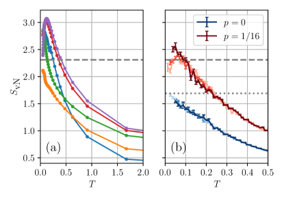
Figure 12: METTS entanglement entropy $S_{\textrm{vN}}$ on the $32\times 4$ cylinder at $U/t=10$ (a) entanglement growth upon time evolving five different product states for $p=1/16$ with $D_{\max}=4000$. (b) Average entanglement entropy $S_{\textrm{vN}}$ of the METTS state as a function of temperature for $p=0$ and $p=1/16$ . Increasing opacity signifies increasing maximal bond dimensions $D_{\max}=2000,3000,4000$. We observe a small peak in the entanglement entropy in the hole-doped case at $T/t\approx 0.05$. The entanglement entropy is converged as a function of bond dimension. The dashed (dotted) lines indicate the entanglement entropy from ground state DMRG with $D_{\max}=4000$ at $p=1/16$ ($p=0$).

X Validation with TPQ and AFQMC

To assess the validity of the METTS calculations across a broad range of temperatures and different dopings, we compare to current state-of-the-art methods. First, we focus on computing the thermodynamic energy $E$, specific heat $C$, and magnetic susceptibility $\chi_{\textrm{m}}$. The method of thermal pure quantum (TPQ) states Sugiura and Shimizu (2012, 2013) has been proven effective to extend the range of system sizes accessible via Exact Diagonalization techniques Wietek et al. (2019); Yamaji et al. (2014); Steinigeweg et al. (2016); Honecker et al. (2020). It is also closely related to the finite-temperature Lanczos method Jaklic and Prelovšek (1994).

The main idea of the TPQ method is that the trace of any operator $\mathcal{O}$ can be evaluated by,

$$\operatorname{Tr}(\mathcal{O})=\mathcal{D}\,\overline{\braket{r}{\mathcal{O}}{r}}.$$ (43)

Here, $\mathcal{D}$ denotes the dimension of the Hilbert space and $\overline{\cdots}$ denotes averaging over normalized random vectors $\ket{r}$. The coefficients of $\ket{r}$ are independent and normally distributed. This is used to evaluate thermal averages as,

$$\braket{\mathcal{O}}=\overline{\braket{\beta}{\mathcal{O}}{\beta}}/\overline{\braket{\beta}{\beta}},$$ (44)

where the TPQ state $\ket{\beta}$ is given by,

$$\ket{\beta}=\text{e}^{-\beta H/2}\ket{r}.$$ (45)

We notice that this state closely resembles the METTS $\ket{\psi_{i}}$ in Eq. 20. The random states $\ket{r}$, however, are not product states and are highly entangled in general. The TPQ state $\ket{\beta}$ can be evaluated using Lanczos techniques Lanczos (1950); Hochbruck and Lubich (1997). Interestingly, the statistical error when random sampling over a finite number $R$ of states is related to the free-energy density at a given temperature Hams and De Raedt (2000); Goldstein et al. (2006) and can be shown to become exponentially small when increasing the system size Sugiura and Shimizu (2012, 2013). We refer the reader to Ref. Wietek et al. (2019); Wietek and Läuchli (2018) for an in-depth explanation of the method.

Apart from a statistical error, the TPQ method has no systematic error and does not apply approximations. It is, however, limited to system sizes for which the Lanczos algorithm can be currently applied. Here, we compare data from METTS and TPQ obtained on a $W=4$ and $L=4$ cylinder. This system size is beyond the reach of numerical full diagonalization of the Hamiltonian matrix. The choice of a $W=4$ cylinder poses a challenge to the METTS calculations due to the long-range nature of the interactions. We think that this benchmark addresses the key difficulties to be overcome in order to simulate longer length cylinders. Also, the case of $p=1/8$ hole-doping is afflicted by a sign-problem when investigated using conventional QMC methods. We show results in Fig. 11. The METTS calculations have been performed with a cutoff $\varepsilon=10^{-6}$ and maximum bond dimension $D_{\max}=2000$. We find agreement within errorbars between TPQ and METTS. For TPQ we have used $R=200$ random vectors.

When comparing to exact results from TPQ, we are limited in system size. At half-filling, however, the auxiliary-field quantum Monte Carlo (AFQMC) method Blankenbecler et al. (1981); White et al. (1989); Honma et al. (1995); Sugiyama and Koonin (1986); Sorella et al. (1989); Gubernatis et al. (2016) can be applied without encountering a sign problem that allows for investigating larger lattice sizes. AFQMC at half-filling also does perform any approximation. We compare spin-correlation functions from METTS and AFQMC at various temperatures on t $32\times 4$ cylinder in Fig. 13. Again, we employed a cutoff $\varepsilon=10^{-6}$ and a maximum bond dimension $D_{\max}=2000$ to perform the time-evolution in METTS.We find agreement within errorbars.

The comparisons in Figs. 11 and 13 show, that METTS agrees with current state-of-the-art unbiased numerical methods whenever they are applicable. We also find, that a maximum bond dimension $D_{\max}=2000$ and a cutoff $\varepsilon=10^{-6}$ in the TDVP time evolution are sufficient to obtain consistent results. The comparison between METTS and TPQ shows, that METTS is reliable at finite doping. The comparison to AFQMC, on the other hand, shows that our implementation of METTS yields consistent results when considering larger lattices.

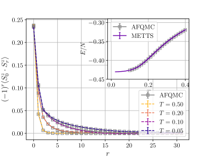
Figure 13: Comparison of spin-correlation functions $\langle S^{z}_{0}\cdot S^{z}_{r}\rangle$ along one leg of a $32\times 4$ cylinder at half-filling and internal energy density $E/N$ between METTS and AFQMC. We used a cutoff of $\varepsilon=10^{-6}$ and a maximum bond dimension $D_{\max}=2000$ for imaginary-time evolution in METTS. Both quantities agree within errorbars. A comparison of the specific heat is shown in Fig. 6(a).

XI Incommensurate spin correlations at $U/t=6$, $p=1/8$, $t^{\prime}/t=-0.25$ and $T/t=0.22$

Determinantal quantum Monte Carlo (DQMC) simulations of the hole-doped Hubbard Model in the strong coupling regime have been reported for the single-band Huang et al. (2018) and three-band Huang et al. (2017) case. These studies have demonstrated the presence of incommensurate spin correlations in the intermediate temperature regime, suggestive of fluctuating stripes. In Ref. Huang et al. (2018) a $16\times 4$ cylindrical geometry was studied for an interaction strength of $U/t=6$, hole-doping $p=1/8$, and temperature $T/t=0.22$. In addition to nearest-neighbor hopping $t$, a second nearest neighbor hopping of size $t^{\prime}/t=-0.25$ was considered. This geometry and parameter regime is directly accessible with our METTS simulations. Hence, this yields an ideal test case, since the DQMC is exact, aside from statistical and Trotter errors. Also, this particular set of parameters is in the interesting regime of finite-doping, strong coupling, and intermediate temperatures. Results of our simulations are shown in Fig. 14. Indeed, we confirm the presence of incommensurate spin correlations consistent with the DQMC. The sign changes which are observed here are in the tails of the rapidly decaying correlation function, and thus they required substantial statistical averaging of the METTS to observe–here, we used 15000 samples. We find that the width of the antiferromagnetic “domains” (in the correlation function) is $5$, which is exactly what has been found in Huang et al. (2018). Moreover, we show the density profile along the cylinder in Fig. 14(d). Here, we observe the same boundary density fluctuations as reported in Fig. 4 of Ref.Huang et al. (2018). In agreement with their findings, the density profile does not exhibit a charge-density wave pattern. We would like to point out, that Refs. Huang et al. (2017, 2018) referred to the incommensurate spin correlations as “stripes”, while our definition of a stripe refers to intertwined spin and charge ordering. Incommensurate charge correlations are not observed for this particular set of parameters.

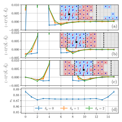
Figure 14: Observation of incommensurate spin correlations at $U/t=6$, $p=1/8$, $t^{\prime}/t=-0.25$ and $T/t=0.22$ on the $16\times 4$ cylinder. (a-c) Staggered spin correlations for three different reference sites. $\delta_{y}$ denotes the offset in $y$-direction. The insets show the sign structure of the staggered spin correlations. The spin correlation is considered to have positive/negative sign if it is non-zero by two standard deviations. (d) Number density $n_{i}$ along the length of the cylinder. Our results confirm the findings presented in Fig. 4 of Ref. Huang et al. (2018).

XII Discussion

The results from the METTS simulations presented in the previous sections yield several interesting new insights into the physics of Hubbard model in the strong coupling regime at $U/t=10$ at finite temperature.

For the hole-doped case at $p=1/16$ we find three different regimes as a function of temperature. At temperatures $T/t\lesssim 0.05$ we find a stripe ordered phase. A typical METTS state in this phase is shown in Fig. 1(a). We observe antiferromagnetic domains whose domain walls coincide with peaks in the wave-like hole density modulation. In the present situation the stripes are half-filled. On a width-$4$ cylinder there are two holes per stripe wavelength. This leads to a magnetic ordering vector of $\bm{k}=(7\pi/8,\pi)=(\pi-\pi/8,\pi)$ and a charge ordering vector of $\bm{k}=(\pi/4,0)$ (hence $\delta\bm{k}_{c}=2\delta\bm{k}_{s}$). This observation agrees well with recent DMRG results on the width-$4$ cylinders Jiang et al. (2020). Even though the exact value of $U/t=10$ and $p=1/16$ is not included in the results of these authors, their phase diagrams suggest that this point realizes what is referred to as the Luther-Emery 1 (LE1) phase at $T=0$. The LE1 phase is shown to exhibit half-filled stripes, in agreement with our findings. The phase diagrams in Ref. Jiang et al. (2020) have been established using DMRG with bond dimensions $D=5000$, which is also the maximal bond dimension we have used in our DMRG calculations. Both the magnetic and the charge structure factors shown in Figs. 2 and 3 clearly indicate the occurrence of stripe order below $T/t\lesssim 0.05$. We would like to mention that a similar crossover from an incommensurate to an antiferromagnetic regime has been found to occur in the three dimensional Hubbard model Schäfer et al. (2017).

At temperatures above the stripe order, we find enhanced antiferromagnetic correlations. As shown in Fig. 4, the spin gap is estimated as $\Delta_{\textrm{s}}/t=0.07$ which approximately coincides with the onset temperature of the stripe order. Around this temperature the peak in the magnetic structure factor shifts from $\bm{k}=(7\pi/8,\pi)$ to $\bm{k}=(\pi,\pi)$. The transition or crossover between the two phases is further signalled by a step-like feature of the specific heat in Fig. 6(b). Hence, we identified several quantities that indicate a transition or crossover between the stripe ordered phase and a phase with enhanced antiferromagnetic correlations but no charge ordering.

The system at $p=1/16$ differs significantly from the antiferromagnetic insulator at half-filling. The density structure factor at zero temperature in Fig. 2(c) indicates a small or vanishing charge gap by exhibiting approximately linear behavior at $\bm{k}=(0,0)$ Feynman (1954); Capello et al. (2005); Tocchio et al. (2011); De Franco et al. (2018); Szasz et al. (2020). We distinguish between the single-particle gap $\Delta_{\textrm{c}}^{(1)}$ and the charge gap $\Delta_{\textrm{c}}^{(2)}$. While the single-particle gap is shown in Fig. 4 to attain a finite value of $\Delta_{\textrm{c}}^{(1)}/t\approx 0.25$ for infinite cylinder length, the charge gap is shown to vanish as $\Delta_{\textrm{c}}^{(2)}/t\propto 1/L$.

Due to the finite single-particle gap, the system does not exhibit a Fermi surface. This is also evident in the momentum distribution function $n_{\sigma}(\bm{k})$ shown in Fig. 5(a), whose slope at $T=0$ remains finite for $p=1/16$, as expected for a system without a Fermi surface Luttinger (1960). We find that for momentum $k_{y}=\pi/2$ the slope of $n_{\sigma}(\bm{k})$ becomes largest close to the nodal point $\bm{k}=(\pi/2,\pi/2)$, indicating that the single-particle gap is smallest in this region. To further corroborate this finding we found that the real space electronic correlations Fourier transformed along the $y$-direction, $\mathcal{F}_{y}(x_{l},x_{m},k_{y})$ in Fig. 5(b), exhibit fast exponential decay at $k_{y}=0,\pi$. At $k_{y}=\pi/2$ a slower exponential decay is observed. Therefore, we conclude that while the single-particle gap is still sizeable, the smallest gap to single particle excitations is realized in the nodal region around $\bm{k}=(\pi/2,\pi/2)$.

The novel short-range antiferromagnetic phase shares many features with the experimentally observed pseudogap region, which is characterized by a partial suppression of low-energy excitations Norman et al. (2005); Alloul (2014); Kordyuk (2015). In particular, angle-resolved photo emission spectroscopy measurements Damascelli et al. (2003) typically detect a suppression of single-particle excitations close to the antinode, $\bm{k}=(\pi,0)$. Similarly, we find in Fig. 5 that the single-particle gap in our case is largest for $y$-momenta $k_{y}=0$ and $k_{y}=\pi$, while it is smallest at $k_{y}=\pi/2$.

The onset temperature $T^{*}$ of the pseudogap phase was originally identified experimentally as a decrease of the uniform magnetic susceptibility upon cooling below $T^{*}$ Alloul et al. (1989); Johnston (1989). In our simulations at $U/t=10$ and $p=1/16$ we indeed detect a maximum in the magnetic susceptibility at $T^{*}/t\approx 0.25$ in Fig. 6. Below this temperature the onset of antiferromagnetic correlations with $(\pi,\pi)$ wave-vector in Fig. 3 agrees well with previous results from cluster extensions of DMFT Macridin et al. (2006); Kyung et al. (2006); Gunnarsson et al. (2015); Chen et al. (2017); Scheurer et al. (2018) and diagrammatic Monte Carlo Wu et al. (2017), which indicate emerging short-range antiferromagnetic correlations in the pseudogap phase.

However, these approaches also point at metallic behaviour in the pseudogap regime, with gapless quasiparticles in the nodal region of the Brillouin zone. Gapless quasiparticles at the node are also expected for superconducting order with $d_{x^{2}-y^{2}}$ symmetry. In contrast, we find a non-vanishing single-particle gap which, although smallest close to the node, has a rather large magnitude $\Delta_{\textrm{c}}^{(1)}/t\approx 0.25$. This is also the temperature scale below which we observe the onset of antiferromagnetism. Hence, the short-range antiferromagnetic correlations in the system that we simulate are not associated with a metallic state hosting gapless single-particle excitations. However, we would like to emphasize that our method is limited by only being able to simulate small width cylinders. It would be very interesting to learn how the single-particle gap evolves with cylinder circumference. Currently, ground state DMRG studies of the Hubbard model are possible on width 6 cylinders Ehlers et al. (2017); Qin et al. (2020a), so some additional information on the evolution of the gap with width should be available soon.

An investigation of pairing (correlations) in both the stripe phase and the pseudogap regime would give additional insights. Since this study requires further technical improvements of our method, this question will be addressed in future work. While the single-particle gap we detect might vanish in the full two-dimensional limit, there are also scenarios where the single-particle gap remains finite while the charge gap vanishes. This behavior is expected for superconductors with a nodeless gap function. Another intriguing possibility is an exotic metallic state, where the electrons fractionalize into chargons and spinons Chatterjee and Sachdev (2016); Else et al. (2020). In this case, the single-particle gap would correspond to the spinon gap while chargons are still gapless.

We have also investigated the half-filled case at $U/t=10$. We find that the magnetic structure factor converges smoothly towards the DMRG result when lowering the temperature in Fig. 2(a). It exhibits a clear peak at $\bm{k}=(\pi,\pi)$ indicating antiferromagnetism. We use the maximum of the static magnetic susceptibility in Fig. 6 at $T^{\times}/t\approx 0.29$ to define an onset temperature of antiferromagnetic correlations. The quadratic behavior we observe for the specific heat at low temperatures is in agreement with thermodynamics derived from antiferromagnetic spin-wave theory  Kubo (1952); Dyson (1956); Yamamoto and Noriki (2019). We have also found that the thermodynamics at half-filling matches closely with quantum Monte Carlo results of the square lattice Heisenberg antiferromagnet Okabe and Kikuchi (1988); Miyashita (1988). In particular, the temperature of the maximum in the specific heat in Fig. 6 agrees well with those QMC results Okabe and Kikuchi (1988); Miyashita (1988).

To the best of our knowledge, this work constitutes the first application of the METTS algorithm to study the Fermi-Hubbard model on geometries approaching the two-dimensional limit. Therefore, we have investigated the behavior of the algorithm in proper detail. We presented the statistical properties of the measurement time series in appendix A. As METTS is a Markov chain Monte Carlo algorithm, it is crucial to understand autocorrelation and thermalization properties. As we have shown in Fig. 15 the time series can indeed take rather long times to thermalize. At half-filling we found that there can be metastable states with multiple antiferromagnetic domains that are realized before the system becomes thermalized. Interestingly, we find that upon hole-doping the system, the measurement time series equilibrate faster. We also investigated autocorrelation effects. We find that applying the $S^{x}$ instead of the $S^{z}$ updates described in section VII.4 reduces the autocorrelation times significantly, as shown in Fig. 16. For the temperatures and observables $\mathcal{O}$ investigated in this manuscript using the $S^{x}$ update, we find autocorraletion time $\tau[\mathcal{O}]\approx 1$. We find that for $T/t\leq 0.5$ for $U/t=10$ and a $32\times 4$ cylinder autocorrelation effects are negligible for most observables. A noticeable exception is the charge density structure factor at temperatures above $T/t\gtrsim 0.20$ shown in Fig. 3(b) where moderate autocorrelation effects have to be taken into account to compute proper error estimates.

The statistical error estimate, apart from the number of samples and the autocorrelation time, also depends on the variance of the time series. We have investigated the behavior of the variance of several observables as a function of temperature in Figs. 17 and 18 and found rather remarkable behavior. The variance of several estimators decreases rapidly when lowering temperatures. Also, increasing the system size decreases the variance of the energy density estimators. This observation is likely related to the phenomenon called quantum typicality Goldstein et al. (2006). For the related thermal pure quantum states (TPQ), which we have used to validate the METTS results in section X, a theory of their statistical properties has been developed in Refs. Sugiura and Shimizu (2012, 2013). The TPQ and METTS states are obtained by imaginary-time evolving states drawn from some class of random initial states. Whereas for a METTS the random initial states are product states, the initial state of a TPQ state is state with (normally distributed) random coefficients in an arbitrary orthonormal basis of the Hilbert space. For the latter, it has been found that the statistical error when averaging over several TPQ states becomes exponentially small in the system size, under mild assumptions on the system and observables. It would be interesting to arrive at a similar understanding of the variance of METTS states to explain our observations. Several methods have been proposed to further improve upon the variance of the estimators Chen and Stoudenmire (2020); Chung and Schollwöck (2019); Iwaki et al. (2020). Refs. Chen and Stoudenmire (2020); Chung and Schollwöck (2019) proposed a hybrid approach interpolating between purification and METTS sampling. While using additional auxiliary sites for purification are likely to increase the necessary bond dimensions of the MPS to achieve convergence, they are favorable in the sense that fewer random states have to be sampled. Especially at higher temperatures, these approaches might yield a significant computational speedup. Also, approaches to incorporate additional symmetries in the METTS algorithm have been proposed Binder and Barthel (2017); Bruognolo et al. (2015). We would also like to mention that several other tensor network approaches to finite temperature simulations have recently been applied successfully to a variety of problems Li et al. (2020); Chen et al. (2018, 2019, 2020); Czarnik and Corboz (2019).

Apart from the statistical analysis, the METTS method relies on accurate imaginary-time evolution algorithms. We find that the TDVP algorithm for time-evolving matrix product states is an appropriate choice. However, the projection error when applying TDVP directly to MPS of small bond dimension, especially product states, is not negligible. We circumvent this problem by applying an initial TEBD time-evolution up to a certain imaginary-time, thus increasing the bond dimension before applying the TDVP algorithm. We find that this approach yields very accurate results compared to numerically exact Lanczos time evolutions. Also, when fixing a maximal bond dimension, we apply single-site TDVP, which has favorable computational costs. We would like to point out that recently a different approach to solving the projection error problem of TDVP has been proposed Yang and White (2020), which employs a subspace expansion using a global Krylov basis.

Simulating the doped Fermi-Hubbard model at finite-temperature poses a challenging problem for numerical methods. To demonstrate the accuracy of our simulations we have performed comparisons to four different well-established exact numerical methods in their respective limits. First, the limit $T/t\rightarrow 0$ is compared to ground state DMRG calculations in Fig. 2. We find that the METTS simulations of the structure factors at $T/t=0.025$ very closely resemble the ground state result from DMRG. This also shows, that for the investigated system our METTS simulations can essentially cover the temperature range down to temperatures which can be considered to realize ground state physics. Second, we have compared thermodynamics at half-filling and finite hole-doping on a $4\times 4$ cylinder to the TPQ method Sugiura and Shimizu (2012, 2013); Wietek et al. (2019) over a large range of temperatures. The TPQ method is an extension of exact diagonalization, where traces over statistical density matrices are replaced by random averages of random vectors. The method is considered to be statistically exact. Also here, we find perfect agreement to METTS shown in Fig. 11. Together with the comparison to DMRG this shows, that METTS yields accurate results at finite hole-doping over the full range of temperatures investigate. Finally, we also demonstrated in Fig. 13 that at half-filling METTS simulations of spin-correlations agree within error bars to statistically exact AFQMC simulations on larger system sizes. Finally, we confirm previous results Huang et al. (2018) by determinantal quantum Monte Carlo obtained in the challenging parameter set $U/t=6$, $p=1/8$, $t^{\prime}/t=-0.25$, and $T/t=0.22$ on a $16\times 4$ cylinder. We correctly reproduce the incommensurate spin correlations and boundary density fluctuations found earlier.

XIII Conclusion

Using the numerical METTS method, we have investigated finite temperature properties of the doped Hubbard model in the strong coupling regime on a width-$4$ cylinder. We focused on hole-doping $p=1/16$ and half-filling. In the doped case we find that the ground state half-filled stripe phase extends up to a temperature $T/t\lesssim 0.05$. Above this temperature, a phase with strong antiferromagnetic correlations is realized. In this regime, the specific heat exhibits behavior linear in $T$. The onset temperature of the short-range stripe order coincides with the spin gap, which has been shown to attain a finite value. A closer inspection of electronic correlations revealed that no full electron-like Fermi surface is realized, however. Instead, we find a vanishingly small gap to paired charge excitations, while the single particle gap of size $\Delta_{\textrm{c}}^{(1)}/t\approx 0.26$ is still sizeable. By investigating the momentum distribution function and electron correlation functions we establish that the single-particle gap is smallest in the nodal region close to $\bm{k}=(\pi/2,\pi/2)$. The magnetic susceptibility realizes a maximum at temperature $T^{*}=0.25t$. These features are strongly reminiscent of the pseudogap phase realized in the cuprates. These findings have been made possible by combining recent tensor network techniques to simulate finite-temperature quantum systems and perform imaginary-time evolution of matrix product states. We found that both increasing the system size as well as lowering the temperature significantly reduces the variance of the METTS estimators, hence reducing the need to average over many random samples. Apart from benchmarking the time-evolution with numerical exact diagonalization, we validated our simulations by comparing to four different numerical methods, DMRG, TPQ, AFQMC, and DQMC. These comparisons demonstrate that systems of strongly-correlated fermions at low temperatures, finite-hole doping, and on large lattice sizes can now be reliably simulated using the METTS method.

Appendix A Time series analysis

Figure 15: Time series of energy and magnetic structure factor measurements from $5$ different random intial states. Data shown for a $32\times 4$ cylinder with parameters $T/t=0.300$, $U/t=10$. We used time evolution parameters $D_{\max}=3000$ and $\varepsilon=10^{-6}$ and $S^{x}$ collapses. After initial thermalization no autocorrelation effects are apparent. (a) energy measurements at half-filling, $p=0$. We observe several initial plateaux in the energy before thermalization. These plateaux are metastable states that correspond to antiferromagnetic domains. (b) energy measurements at hole-doping $p=1/16$. (c,d) measurements of the magnetic structure factor $S(\bm{k})$ evaluated at ordering vector $\bm{k}=(\pi,\pi)$ at $p=0$ and $p=1/16$. We observe a skewed distribution, fast thermalization and no apparent autocorrelation effects.

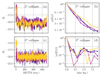
Figure 16: Comparison of energy time series and autocorrelation functions $\rho[H](l)$ obtained using $S^{z}$ and $S^{x}$ collapses for $T/t=0.400$, $U/t=10$ at half-filling on a $16\times 4$ cylinder. We used time evolution parameters $D_{\max}=2000$ and $\varepsilon=10^{-6}$. (a,b): $S^{z}$-basis collapse. Autocorrelation effects are visible in the raw data. (c,d): $S^{x}$-basis collapse. No autocorrelation effects are apparent in the timeseries. The autocorrelation function quickly decays to numerical noise. Subsequent measurements are essentially uncorrelated.

In this section, we discuss the statistical properties of the METTS sampling. As described in section VII.1, the METTS algorithm is an example of a Markov chain Monte Carlo simulation. As such, thermalization and autocorrelation properties of the resulting time series have to be investigated to derive (error) estimates of physical observables. We find that the behavior of the METTS algorithm as a function of temperature is quite opposite to usual quantum Monte Carlo simulations. Thermalization and autocorrelation times decrease when lowering the temperature. Eventually, using the $S^{x}$-basis collapse instead of the $S^{z}$-basis collapse, as discussed in section VII.4, we find that autocorrelation effects can be neglected for the temperature range we study. We also show that the variance of several quantities decreases quickly for lower temperatures. This allows reaching a higher statistical precision at lower temperatures, where imaginary-time evolution is more computationally expensive.

For an observable $\mathcal{O}$ the METTS algorithm yields a time series of measurements,

$$\mathcal{O}_{i}=\braket{\psi_{i}}{\mathcal{O}}{\psi_{i}},\quad i=1,\ldots,R.$$ (46)

The thermal average $\braket{\mathcal{O}}$ in Eq. 2 is then estimated by

$$\braket{\mathcal{O}}\approx\text{E}[\mathcal{O}]=\frac{1}{R}\sum_{i=1}^{R}\mathcal{O}_{i}.$$ (47)

The individual samples $\mathcal{O}_{i}$ are, in general, correlated. Averages in Eq. 47 are computed after the initial thermalization of the measurements. An estimate of the standard error $\sigma[\mathcal{O}]$ of Eq. 47 is given by Sokal (1997); Ambegaokar and Troyer (2010),

$$\sigma[\mathcal{O}]\approx\sqrt{\frac{\tau[\mathcal{O}]}{R}\text{Var}[\mathcal{O}]}.$$ (48)

Here, $\text{Var}[\mathcal{O}]$ denotes an estimator for the variance,

$$\text{Var}[\mathcal{O}]=\frac{1}{R-1}\sum_{i=1}^{R}(\mathcal{O}_{i}-\text{E}[\mathcal{O}])^{2},$$ (49)

$\tau[\mathcal{O}]$ denotes an estimator for the integrated autocorrelation time,

$$\tau[\mathcal{O}]=1+2\sum_{l=1}^{M}\frac{\rho[\mathcal{O}](l)}{\rho[\mathcal{O}](0)},$$ (50)

and the estimated autocorrelation function $\rho[\mathcal{O}](l)$ is given by Ambegaokar and Troyer (2010),

$$\rho[\mathcal{O}](l)=\frac{1}{R-l}\sum_{i=1}^{R-l}(\mathcal{O}_{i}-\text{E}[\mathcal{O}])(\mathcal{O}_{i+l}-\text{E}[\mathcal{O}]).$$ (51)

The autocorrelation function $\rho[\mathcal{O}](l)$ is typically exponentially decaying in $l$. The cutoff value $M\propto\tau[\mathcal{O}]$ is chosen such to assure convergence of the sum in Eq. 50, but small enough not to include numerical noise. For a proper choice of $M$, see Ref. Sokal (1997).

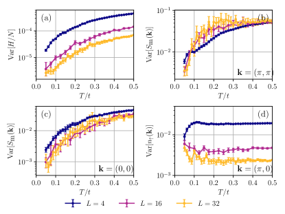
Figure 17: Lattice size and temperature dependence of the variance of time series of METTS measurements for $U/t=10$ and hole-dopings $p=1/8$ cylinder for $L=4,16,32$. We used time evolution parameters $D_{\max}=2000$ and $\varepsilon=10^{-6}$. Error bars indicate a $95\%$ confidence interval. (a) Energy measurements. We observe a fast decrease of the variance as lowering temperature. (b) Magnetic structure factor $S(\bm{k})$ at ordering vector $\bm{k}=(\pi,\pi)$. (c) Magnetic structure factor $S(\bm{k})$ at $\bm{k}=(0,0)$. (d) momentum distribution function $n_{\uparrow}(\bm{k})$ at $\mathbf{k}=(\pi,0)$.

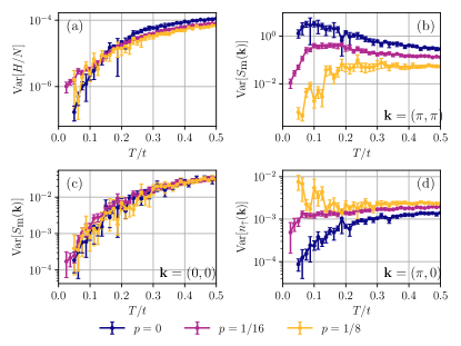
Figure 18: Variance of time series of METTS measurements for $U/t=10$ for hole-dopings $p=0,1/16,1/8$ on a $32\times 4$ cylinder. We used time evolution parameters $D_{\max}=3000$ and $\varepsilon=10^{-6}$. Error bars indicate a $95\%$ confidence interval. (a) Energy measurements. We observe a fast decrease of the variance as lowering temperature. (b) Magnetic structure factor $S(\bm{k})$ at ordering vector $\bm{k}=(\pi,\pi)$. (c) Magnetic structure factor $S(\bm{k})$ at ordering vector $\bm{k}=(0,0)$. (d) momentum distribution function $n(\bm{k})$ at reciprocal vector $\bm{k}=(\pi,0)$.

We show examples of the measurement time series for different quantities in Fig. 15. We choose a temperature of $T/t=0.300$ and Hubbard interaction $U/t=10$ on a $32\times 4$ cylinder. The imaginary-time evolution has been performed with TDVP cutoff $\varepsilon=10^{-6}$ and maximum bond dimension $D_{\max}=3000$. We used the $S^{x}$ basis collapse scheme. For energy measurements in the half-filled case in Fig. 15(a) we see that several hundred steps can be required to thermalize the system. Before reaching equilibrium, the METTS algorithm is temporarily stuck in metastable states. By a closer inspection of these states, we find that they typically contain several antiferromagnetic domains instead of a uniform antiferromagnetic state, which is realized once the system is thermalized at this temperature $T/t=0.300$. We consistently find this behavior for temperatures $T/t\geq 0.200$. We observe that the time for thermalization decreases when lowering the temperature. This is explained by the fact that a longer imaginary-time evolution constitutes a more thorough update to the Monte Carlo algorithm, hence improving the mixing properties of the Markov chain. Similarly, the measurements of the magnetic structure factor $S(\bm{k})$ evaluated at ordering vector $\bm{k}=(\pi,\pi)$ in Fig. 15(c) exhibit prolonged thermalization at half-filling, although less pronounced than for the energy measurements. Fig. 15(b) shows the energy measurement time series for a $32\times 4$ cylinder with $T/t=0.300$, $U/t=10$, $L=32$ at hole-doping $p=1/16$. Interestingly, no initial metastable plateaux are observed and the system thermalizes more rapidly than in the half-filled case. This could be explained by the additional charge fluctuations “smoothing” the energy landscape around the metastable antiferromagnetic domain states. Fig. 15(d) shows measurements of $S(\bm{k})$ at $\bm{k}=\textrm{M}$ for $p=1/16$. Also for this observable, the system is quickly thermalized. The distributions of the magnetic structure factors in Fig. 15(c) and (d) are skewed.

After an initial period of thermalization, we do not observe apparent autocorrelation effects in all time series shown in Fig. 15. This is owed to the fact, that the $S^{x}$-basis collapses reduce the autocorrelation time substantially as compared to $S^{z}$-basis updates. In Fig. 16 we compare the two collapse strategies for $T/t=0.400$, $U/t=10$, $L=16$, and $W=4$ at half-filling. As shown in Fig. 16(a) and (b), the energy time series shows significant autocorrelation effects when applying the $S^{z}$-basis collapse. This is characterized by the autocorrelation time, estimated here as $\tau[H]=9.46$. Using $S^{x}$-basis collapses instead, we find that subsequent samples are essentially uncorrelated, as shown in Fig. 16(c) and (d). There, we estimate an autocorrelation time of $\tau[H]\approx 1.08$.

Apart from the autocorrelation time and the number of random samples $R$, the statistical error estimate in Eq. 48 is determined by the variance of the measurements, $\text{Var}[\mathcal{O}]$. While the number of random samples $R$ can be adjusted to achieve a fixed statistical error $\sigma[\mathcal{O}]$, both the autocorrelation time and the variance are intrinsic properties of the observable and the METTS algorithm. We investigate the behavior of the variance for several quantities in Figs. 17 and 18. We estimated a $95\%$ confidence interval for the variance estimator Eq. 49 using bootstrap resampling Efron (1979). Fig. 17 compares variances for different system sizes and temperatures at hole-doping $p=1/8$. Remarkably, we find that both decreasing temperature as well as increasing the system size decreases the variance of the energy density considerably, cf. Fig. 17(a). Low temperatures and large system sizes are of course the more challenging regimes to perform the MPS time evolution. Hence, in order to achieve comparable statistical error estimates, less MPS time evolutions have to be performed. Similarly, we observe in Fig. 17(b,c) that the variance of the magnetic structure factor evaluated at $\bm{k}=(0,0)$ and $\bm{k}=(\pi,\pi)$ decreases as a function of temperature. Also for the momentum distribution function at $\bm{k}=(\pi,0)$ in Fig. 17(d) we observe that increasing the system size decreases the variance.

We compare estimators of variances at different hole-dopings in Fig. 18. The energy and magnetic structure factor of $\bm{k}=(0,0)$ variances in Fig. 18(a,c) do not depend strongly on the filling fraction. We observe a rapid decrease of the variance when lowering the temperature. In contrast, the variance of the magnetic structure factor evaluated at $\textrm{M}=(\pi,\pi)$ in Fig. 18(b) does not rapidly decrease at half-filling. This can be attributed to the fact, that $S(\bm{k})$ develops a peak at $\bm{k}=(\pi,\pi)$ at low temperatures indicating the development of strong antiferromagnetic correlations. The variance of the momentum $n(\bm{k})$ distribution function evaluated at $\bm{k}=(\pi,0)$ also shows interesting behavior in Fig. 18(d). The variance is largest for hole-doping $p=1/8$, contrary to the magnetic structure factor.

Appendix B Numerical differentiation using total variation regularization

In the main text, we compute the specific heat as the derivative of the total energy w.r.t. the temperature,

$$C=\frac{\textrm{d}E}{\textrm{d}T}.$$ (52)

The energy is computed using METTS sampling and is hence afflicted by a statistical error $\delta$. When performing a numerical finite-difference with spacing $h$, the straightforward error estimate is proportional to $\delta/h$ and hence diverges as $h\rightarrow 0$.

An established way to estimate derivatives of noisy data is to perform total variation regularization Chartrand (2011). Crudely speaking, the total variation of a function is a measure of how rapidly it oscillates. More precisely, the total variation of a differentiable function of one variable $u$ is given by,

$$\textrm{TV}[u]=\int|u^{\prime}|\;,$$ (53)

where the prime denotes its derivative. We would like to point out that this corresponds to the $L^{1}$-norm of the derivative of $u$ and not the more conventional $L^{2}$-norm. Thermodynamic observables, like the specific heat, are not expected to rapidly oscillate. Therefore, it can be assumed that their total variation is of small magnitude.

We describe the method proposed by Ref. Chartrand (2011). Given a function $f$, we seek to find a regularized derivative $u_{\alpha}$ of $f$, minimizing the functional,

$$F[u]=\alpha\int|u^{\prime}|\;+\frac{1}{2}\int|Au-f|^{2}.$$ (54)

Here, $Au(x)=\int_{0}^{x}u$ denotes the operator of anti-differentiation (assuming $f(0)=0$). The prefactor $\alpha$ is the regularization parameter. A minimizing function $u_{\alpha}$ of $F$ is thus in balance between closely integrating to $f$ and having small total variation. Ref Chartrand (2011) proposes an efficient algorithm to solve this minimization problem, based on the lagged-diffusivity algorithm Vogel and Oman (1996). In our application, $f\hat{=}E$ and $u_{\alpha}\hat{=}C$.

We are given data points $\{f(x_{i})\}_{i=1}^{N}$ with corresponding error estimates $\{\delta f(x_{i})\}_{i=1}^{N}$. To derive an estimate for the regularized derivative $\{u_{\alpha}(x_{i})\}_{i=1}^{N}$ and its standard deviation $\{\delta u(x_{i})\}_{i=1}^{N}$, we apply a simple bootstrap idea. We randomly sample datapoints according to normal distributions with mean $f(x_{i})$ and standard deviation $\delta f(x_{i})$. For every random sample we compute the regularized derivative by minimizing Eq. 54. From those samples of regularized derivatives we then estimate the mean and standard deviation. We use $R=100$ random samples to perform these estimates.

References

- Bednorz and Müller (1986) J George Bednorz and K Alex Müller, “Possible high superconductivity in the Ba-La-Cu-O system,” Z. Phys. B Condens. Matter 64, 189–193 (1986).
- Orenstein and Millis (2000) J. Orenstein and A. J. Millis, “Advances in the Physics of High-Temperature Superconductivity,” Science 288, 468–474 (2000).
- Lee, P.A. and Nagaosa, N. and Wen, X.G. (2006) Lee, P.A. and Nagaosa, N. and Wen, X.G., “Doping a Mott insulator: Physics of high-temperature superconductivity,” Rev. Mod. Phys. 78, 17–85 (2006).
- Imada et al. (1998) Masatoshi Imada, Atsushi Fujimori, and Yoshinori Tokura, “Metal-insulator transitions,” Rev. Mod. Phys. 70, 1039–1263 (1998).
- Keimer et al. (2015) B. Keimer, S. A. Kivelson, M. R. Norman, S. Uchida, and J. Zaanen, “From quantum matter to high-temperature superconductivity in copper oxides,” Nature 518, 179–186 (2015).
- Norman et al. (2005) M. R. Norman, D. Pines, and C. Kallin, “The pseudogap: friend or foe of high ?” Adv. Phys. 54, 715–733 (2005).
- Alloul (2014) Henri Alloul, “What is the simplest model that captures the basic experimental facts of the physics of underdoped cuprates?” C. R. Phys. 15, 519 – 524 (2014).
- Benhabib et al. (2015) S. Benhabib, A. Sacuto, M. Civelli, I. Paul, M. Cazayous, Y. Gallais, M.-A. Méasson, R. D. Zhong, J. Schneeloch, G. D. Gu, D. Colson, and A. Forget, “Collapse of the Normal-State Pseudogap at a Lifshitz Transition in the Cuprate Superconductor,” Phys. Rev. Lett. 114, 147001 (2015).
- Loret et al. (2017) B. Loret, S. Sakai, S. Benhabib, Y. Gallais, M. Cazayous, M. A. Méasson, R. D. Zhong, J. Schneeloch, G. D. Gu, A. Forget, D. Colson, I. Paul, M. Civelli, and A. Sacuto, “Vertical temperature boundary of the pseudogap under the superconducting dome in the phase diagram of ,” Phys. Rev. B 96, 094525 (2017).
- Kordyuk (2015) A. A. Kordyuk, “Pseudogap from ARPES experiment: Three gaps in cuprates and topological superconductivity (Review Article),” Low Temp. Phys. 41, 319–341 (2015).
- Vishik et al. (2010) IM Vishik, WS Lee, RH He, M Hashimoto, Z Hussain, TP Devereaux, and ZX Shen, “ARPES studies of cuprate Fermiology: superconductivity, pseudogap and quasiparticle dynamics,” New J. Phys. 12, 105008 (2010).
- Wu et al. (2015) Tao Wu, Hadrien Mayaffre, Steffen Krämer, Mladen Horvatić, Claude Berthier, W. N. Hardy, Ruixing Liang, D. A. Bonn, and Marc-Henri Julien, “Incipient charge order observed by NMR in the normal state of YBa2Cu3Oy,” Nat Comm. 6, 6438 (2015), arXiv:1404.1617 .
- Comin and Damascelli (2016) Riccardo Comin and Andrea Damascelli, “Resonant X-Ray Scattering Studies of Charge Order in Cuprates,” Annu. Rev. 7, 369–405 (2016), arXiv:1509.03313 .
- Anderson (1987) P. W. Anderson, “The Resonating Valence Bond State in \chLa2CuO4 and Superconductivity,” Science 235, 1196–1198 (1987).
- Zhang and Rice (1988) F. C. Zhang and T. M. Rice, “Effective Hamiltonian for the superconducting Cu oxides,” Phys. Rev. B 37, 3759–3761 (1988).
- Emery and Reiter (1988) V. J. Emery and G. Reiter, “Mechanism for high-temperature superconductivity,” Phys. Rev. B 38, 4547–4556 (1988).
- LeBlanc et al. (2015) J. P. F. LeBlanc, A. E. Antipov, F. Becca, I. W. Bulik, Garnet Kin-Lic Chan, C.M. Chung, Y. Deng, M. Ferrero, T.M. Henderson, C.A. Jiménez-Hoyos, E. Kozik, X.W. Liu, A.J. Millis, N.V. Prokof’ev, M. Qin, G.E. Scuseria, H. Shi, B. V. Svistunov, L.F. Tocchio, I.S. Tupitsyn, S.R. White, S. Zhang, B.X. Zheng, Z. Zhu, and E. Gull (Simons Collaboration on the Many-Electron Problem), “Solutions of the Two-Dimensional Hubbard Model: Benchmarks and Results from a Wide Range of Numerical Algorithms,” Phys. Rev. X 5, 041041 (2015).
- Zheng et al. (2017) Bo-Xiao Zheng, Chia-Min Chung, Philippe Corboz, Georg Ehlers, Ming-Pu Qin, Reinhard M. Noack, Hao Shi, Steven R. White, Shiwei Zhang, and Garnet Kin-Lic Chan, “Stripe order in the underdoped region of the two-dimensional Hubbard model,” Science 358, 1155–1160 (2017).
- Qin et al. (2020a) Mingpu Qin, Chia-Min Chung, Hao Shi, Ettore Vitali, Claudius Hubig, Ulrich Schollwöck, Steven R. White, and Shiwei Zhang (Simons Collaboration on the Many-Electron Problem), “Absence of Superconductivity in the Pure Two-Dimensional Hubbard Model,” Phys. Rev. X 10, 031016 (2020a).
- Schäfer et al. (2020) Thomas Schäfer, Nils Wentzell, IV Šimkovic, Fedor, Yuan-Yao He, Cornelia Hille, Marcel Klett, Christian J. Eckhardt, Behnam Arzhang, Viktor Harkov, François-Marie Le Régent, Alfred Kirsch, Yan Wang, Aaram J. Kim, Evgeny Kozik, Evgeny A. Stepanov, Anna Kauch, Sabine Andergassen, Philipp Hansmann, Daniel Rohe, Yuri M. Vilk, James P. F. LeBlanc, Shiwei Zhang, A. M. S. Tremblay, Michel Ferrero, Olivier Parcollet, and Antoine Georges, “Tracking the Footprints of Spin Fluctuations: A Multi-Method, Multi-Messenger Study of the Two-Dimensional Hubbard Model,” arXiv e-prints (2020), arXiv:2006.10769 .
- White (1992) Steven R. White, “Density matrix formulation for quantum renormalization groups,” Phys. Rev. Lett. 69, 2863–2866 (1992).
- White (1993) Steven R. White, “Density-matrix algorithms for quantum renormalization groups,” Phys. Rev. B 48, 10345–10356 (1993).
- Schollwöck (2005) U. Schollwöck, “The density-matrix renormalization group,” Rev. Mod. Phys. 77, 259–315 (2005).
- Schollwöck (2011) Ulrich Schollwöck, “The density-matrix renormalization group in the age of matrix product states,” Annals of Physics 326, 96 – 192 (2011).
- White and Scalapino (1998) Steven R. White and D. J. Scalapino, “Density Matrix Renormalization Group Study of the Striped Phase in the 2D Model,” Phys. Rev. Lett. 80, 1272–1275 (1998).
- White and Scalapino (2003) Steven R. White and D. J. Scalapino, “Stripes on a 6-Leg Hubbard Ladder,” Phys. Rev. Lett. 91, 136403 (2003).
- Hager et al. (2005) G. Hager, G. Wellein, E. Jeckelmann, and H. Fehske, “Stripe formation in doped Hubbard ladders,” Phys. Rev. B 71, 075108 (2005).
- Ehlers et al. (2017) G. Ehlers, S. R. White, and R. M. Noack, “Hybrid-space density matrix renormalization group study of the doped two-dimensional Hubbard model,” Phys. Rev. B 95, 125125 (2017).
- Qin et al. (2020b) Mingpu Qin, Chia-Min Chung, Hao Shi, Ettore Vitali, Claudius Hubig, Ulrich Schollwöck, Steven R. White, and Shiwei Zhang (Simons Collaboration on the Many-Electron Problem), “Absence of Superconductivity in the Pure Two-Dimensional Hubbard Model,” Phys. Rev. X 10, 031016 (2020b).
- Jiang et al. (2020) Yi-Fan Jiang, Jan Zaanen, Thomas P. Devereaux, and Hong-Chen Jiang, “Ground state phase diagram of the doped Hubbard model on the four-leg cylinder,” Phys. Rev. Research 2, 033073 (2020).
- Chang and Zhang (2010) Chia-Chen Chang and Shiwei Zhang, “Spin and charge order in the doped hubbard model: Long-wavelength collective modes,” Phys. Rev. Lett. 104, 116402 (2010).
- Xu et al. (2011) Jie Xu, Chia-Chen Chang, Eric J Walter, and Shiwei Zhang, J. Phys.: Condens. Matter 23, 505601 (2011).
- Tocchio et al. (2011) Luca F. Tocchio, Federico Becca, and Claudius Gros, “Backflow correlations in the Hubbard model: An efficient tool for the study of the metal-insulator transition and the large- limit,” Phys. Rev. B 83, 195138 (2011).
- Knizia and Chan (2012) G. Knizia and Garnet Kin-Lic Chan, “Density Matrix Embedding: A Simple Alternative to Dynamical Mean-Field Theory,” Phys. Rev. Lett. 109, 186404 (2012).
- Knizia and Chan (2013) Gerald Knizia and Garnet Kin-Lic Chan, “Density Matrix Embedding: A Strong-Coupling Quantum Embedding Theory,” J. Chem. Theory Comput. 9, 1428–1432 (2013).
- Zheng and Chan (2016) B. X. Zheng and Garnet Kin-Lic Chan, “Ground-state phase diagram of the square lattice Hubbard model from density matrix embedding theory,” Phys. Rev. B 93, 035126 (2016).
- Huang et al. (2017) Edwin W. Huang, Christian B. Mendl, Shenxiu Liu, Steve Johnston, Hong-Chen Jiang, Brian Moritz, and Thomas P. Devereaux, “Numerical evidence of fluctuating stripes in the normal state of high- cuprate superconductors,” Science 358, 1161–1164 (2017).
- Huang et al. (2018) Edwin W. Huang, Christian B. Mendl, Hong-Chen Jiang, Brian Moritz, and Thomas P. Devereaux, “Stripe order from the perspective of the Hubbard model,” npj Quantum Materials 3, 22 (2018).
- Zaanen and Gunnarsson (1989) Jan Zaanen and Olle Gunnarsson, “Charged magnetic domain lines and the magnetism of high- oxides,” Phys. Rev. B 40, 7391–7394 (1989).
- Machida (1989) Kazushige Machida, “Magnetism in \chLa2CuO4 based compounds,” Physica C: Superconductivity 158, 192 – 196 (1989).
- Kato et al. (1990) Masaru Kato, Kazushige Machida, Hiizu Nakanishi, and Mitsutaka Fujita, “Soliton Lattice Modulation of Incommensurate Spin Density Wave in Two Dimensional Hubbard Model -A Mean Field Study-,” J. Phys. Soc. Japan 59, 1047–1058 (1990).
- Kivelson et al. (2003) S. A. Kivelson, I. P. Bindloss, E. Fradkin, V. Oganesyan, J. M. Tranquada, A. Kapitulnik, and C. Howald, “How to detect fluctuating stripes in the high-temperature superconductors,” Rev. Mod. Phys. 75, 1201–1241 (2003).
- Georges et al. (1996) Antoine Georges, Gabriel Kotliar, Werner Krauth, and Marcelo J. Rozenberg, “Dynamical mean-field theory of strongly correlated fermion systems and the limit of infinite dimensions,” Rev. Mod. Phys. 68, 13–125 (1996).
- Maier et al. (2005) T. A. Maier, M. Jarrell, T. Pruschke, and M. Hettler, “Quantum cluster theories,” Rev. Mod. Phys. 77, 1027–1080 (2005).
- Kotliar et al. (2006) G. Kotliar, S. Y. Savrasov, K. Haule, V. S. Oudovenko, O. Parcollet, and C. A. Marianetti, “Electronic structure calculations with dynamical mean-field theory,” Rev. Mod. Phys. 78, 865–951 (2006).
- Tremblay et al. (2006) A. M. S. Tremblay, B. Kyung, and D. Sénéchal, “Pseudogap and high-temperature superconductivity from weak to strong coupling. Towards a quantitative theory (Review Article),” Low Temperature Physics 32, 424–451 (2006).
- Huscroft et al. (2001) C. Huscroft, M. Jarrell, Th. Maier, S. Moukouri, and A. N. Tahvildarzadeh, “Pseudogaps in the 2D Hubbard Model,” Phys. Rev. Lett. 86, 139–142 (2001).
- Civelli et al. (2005) Marcello Civelli, Massimo Capone, S. S. Kancharla, Olivier Parcollet, and Gabriel Kotliar, “Dynamical breakup of the Fermi surface in a doped Mott insulator,” Phys. Rev. Lett. 95, 106402 (2005).
- Sadovskii et al. (2005) M. V. Sadovskii, I. A. Nekrasov, E. Z. Kuchinskii, Th. Pruschke, and V. I. Anisimov, “Pseudogaps in strongly correlated metals: A generalized dynamical mean-field theory approach,” Phys. Rev. B 72, 155105 (2005).
- Stanescu and Kotliar (2006) Tudor D. Stanescu and Gabriel Kotliar, “Fermi arcs and hidden zeros of the green function in the pseudogap state,” Phys. Rev. B 74, 125110 (2006).
- Haule and Kotliar (2007) Kristjan Haule and Gabriel Kotliar, “Strongly correlated superconductivity: A plaquette dynamical mean-field theory study,” Phys. Rev. B 76, 104509 (2007).
- Zhang and Imada (2007) Y. Z. Zhang and Masatoshi Imada, “Pseudogap and Mott transition studied by cellular dynamical mean-field theory,” Phys. Rev. B 76, 045108 (2007).
- Imada et al. (2013) Masatoshi Imada, Shiro Sakai, Youhei Yamaji, and Yukitoshi Motome, “Theory of Pseudogap in Underdoped Cuprates,” in J. Phys.: Conf. Ser., Vol. 449 (2013) p. 012005.
- Liebsch and Tong (2009) Ansgar Liebsch and Ning-Hua Tong, “Finite-temperature exact diagonalization cluster dynamical mean-field study of the two-dimensional Hubbard model: Pseudogap, non-Fermi-liquid behavior, and particle-hole asymmetry,” Phys. Rev. B 80, 165126 (2009).
- Ferrero et al. (2009) M. Ferrero, P. S. Cornaglia, L. DeLeo, O. Parcollet, G. Kotliar, and A. Georges, “Valence bond dynamical mean-field theory of doped Mott insulators with nodal/antinodal differentiation,” EPL 85, 57009 (2009), arXiv:0806.4383 .
- Ferrero et al. (2009) Michel Ferrero, Pablo S. Cornaglia, Lorenzo De Leo, Olivier Parcollet, Gabriel Kotliar, and Antoine Georges, “Pseudogap opening and formation of Fermi arcs as an orbital-selective Mott transition in momentum space,” Phys. Rev. B 80, 064501 (2009).
- Gull et al. (2010) E. Gull, M. Ferrero, O. Parcollet, A. Georges, and A. J. Millis, “Momentum-space anisotropy and pseudogaps: A comparative cluster dynamical mean-field analysis of the doping-driven metal-insulator transition in the two-dimensional hubbard model,” Phys. Rev. B 82, 155101 (2010).
- Gull et al. (2013) Emanuel Gull, Olivier Parcollet, and Andrew J. Millis, “Superconductivity and the Pseudogap in the Two-Dimensional Hubbard Model,” Phys. Rev. Lett. 110, 216405 (2013).
- Sordi et al. (2012) G. Sordi, P. Sémon, K. Haule, and A. M. S. Tremblay, “Strong Coupling Superconductivity, Pseudogap, and Mott Transition,” Phys. Rev. Lett. 108, 216401 (2012).
- Reymbaut et al. (2019) A. Reymbaut, S. Bergeron, R. Garioud, M. Thénault, M. Charlebois, P. Sémon, and A. M. S. Tremblay, “Pseudogap, van hove singularity, maximum in entropy, and specific heat for hole-doped mott insulators,” Phys. Rev. Research 1, 023015 (2019).
- Preuss et al. (1997) R. Preuss, W. Hanke, C. Gröber, and H. G. Evertz, “Pseudogaps and Their Interplay with Magnetic Excitations in the Doped 2D Hubbard Model,” Phys. Rev. Lett. 79, 1122–1125 (1997).
- Macridin et al. (2006) Alexandru Macridin, M. Jarrell, Thomas Maier, P. R. C. Kent, and Eduardo D’Azevedo, “Pseudogap and Antiferromagnetic Correlations in the Hubbard Model,” Phys. Rev. Lett. 97, 036401 (2006).
- Kyung et al. (2006) B. Kyung, S. S. Kancharla, D. Sénéchal, A. M. S. Tremblay, M. Civelli, and G. Kotliar, “Pseudogap induced by short-range spin correlations in a doped Mott insulator,” Phys. Rev. B 73, 165114 (2006).
- Gunnarsson et al. (2015) O. Gunnarsson, T. Schäfer, J. P. F. LeBlanc, E. Gull, J. Merino, G. Sangiovanni, G. Rohringer, and A. Toschi, “Fluctuation Diagnostics of the Electron Self-Energy: Origin of the Pseudogap Physics,” Phys. Rev. Lett. 114, 236402 (2015).
- Wu et al. (2017) Wei Wu, Michel Ferrero, Antoine Georges, and Evgeny Kozik, “Controlling Feynman diagrammatic expansions: Physical nature of the pseudogap in the two-dimensional Hubbard model,” Phys. Rev. B 96, 041105(R) (2017).
- Scheurer et al. (2018) Mathias S. Scheurer, Shubhayu Chatterjee, Wei Wu, Michel Ferrero, Antoine Georges, and Subir Sachdev, “Topological order in the pseudogap metal,” Proc. Natl. Acad. Sci. U.S.A 115, E3665–E3672 (2018).
- Wu et al. (2018) Wei Wu, Mathias S. Scheurer, Shubhayu Chatterjee, Subir Sachdev, Antoine Georges, and Michel Ferrero, “Pseudogap and Fermi-Surface Topology in the Two-Dimensional Hubbard Model,” Phys. Rev. X 8, 021048 (2018).
- Rossi (2017) Riccardo Rossi, “Determinant Diagrammatic Monte Carlo Algorithm in the Thermodynamic Limit,” Phys. Rev. Lett. 119, 045701 (2017).
- Gukelberger et al. (2017) Jan Gukelberger, Evgeny Kozik, and Hartmut Hafermann, “Diagrammatic Monte Carlo approach for diagrammatic extensions of dynamical mean-field theory: Convergence analysis of the dual fermion technique,” Phys. Rev. B 96, 035152 (2017).
- Vučičevic and Ferrero (2020) J. Vučičevic and M. Ferrero, “Real-frequency diagrammatic Monte Carlo at finite temperature,” Phys. Rev. B 101, 075113 (2020).
- White (2009) Steven R. White, “Minimally Entangled Typical Quantum States at Finite Temperature,” Phys. Rev. Lett. 102, 190601 (2009).
- Stoudenmire and White (2010) E M Stoudenmire and Steven R White, “Minimally entangled typical thermal state algorithms,” New Journal of Physics 12, 055026 (2010).
- Verstraete et al. (2004) F. Verstraete, J. J. García-Ripoll, and J. I. Cirac, “Matrix Product Density Operators: Simulation of Finite-Temperature and Dissipative Systems,” Phys. Rev. Lett. 93, 207204 (2004).
- Feiguin and White (2005) A. E. Feiguin and S. R. White, “Finite-temperature density matrix renormalization using an enlarged Hilbert space,” Phys. Rev. B 72, 220401(R) (2005).
- Tiegel et al. (2014) A. C. Tiegel, S. R. Manmana, T. Pruschke, and A. Honecker, “Matrix product state formulation of frequency-space dynamics at finite temperatures,” Phys. Rev. B 90, 060406(R) (2014).
- Becker et al. (2017) J. Becker, T. Köhler, A. C. Tiegel, S. R. Manmana, S. Wessel, and A. Honecker, “Finite-temperature dynamics and thermal intraband magnon scattering in Haldane spin-one chains,” Phys. Rev. B 96, 060403(R) (2017).
- Buser et al. (2019) Maximilian Buser, Fabian Heidrich-Meisner, and Ulrich Schollwöck, “Finite-temperature properties of interacting bosons on a two-leg flux ladder,” Phys. Rev. A 99, 053601 (2019).
- Hauschild et al. (2018) Johannes Hauschild, Eyal Leviatan, Jens H. Bardarson, Ehud Altman, Michael P. Zaletel, and Frank Pollmann, “Finding purifications with minimal entanglement,” Phys. Rev. B 98, 235163 (2018).
- Bruognolo et al. (2017) Benedikt Bruognolo, Zhenyue Zhu, Steven R. White, and E. Miles Stoudenmire, “Matrix product state techniques for two-dimensional systems at finite temperature,” (2017), arXiv:1705.05578 .
- Binder and Barthel (2015) Moritz Binder and Thomas Barthel, “Minimally entangled typical thermal states versus matrix product purifications for the simulation of equilibrium states and time evolution,” Phys. Rev. B 92, 125119 (2015).
- Fishman et al. (2020) Matthew Fishman, Steven R. White, and E. Miles Stoudenmire, “The ITensor software library for tensor network calculations,” (2020), arXiv:2007.14822 .
- Feynman (1954) R. P. Feynman, “Atomic Theory of the Two-Fluid Model of Liquid Helium,” Phys. Rev. 94, 262–277 (1954).
- Capello et al. (2005) Manuela Capello, Federico Becca, Michele Fabrizio, Sandro Sorella, and Erio Tosatti, “Variational Description of Mott Insulators,” Phys. Rev. Lett. 94, 026406 (2005).
- De Franco et al. (2018) Caterina De Franco, Luca F. Tocchio, and Federico Becca, “Metal-insulator transitions, superconductivity, and magnetism in the two-band Hubbard model,” Phys. Rev. B 98, 075117 (2018).
- Szasz et al. (2020) Aaron Szasz, Johannes Motruk, Michael P. Zaletel, and Joel E. Moore, “Chiral Spin Liquid Phase of the Triangular Lattice Hubbard Model: A Density Matrix Renormalization Group Study,” Phys. Rev. X 10, 021042 (2020).
- Luttinger (1960) J. M. Luttinger, “Fermi Surface and Some Simple Equilibrium Properties of a System of Interacting Fermions,” Phys. Rev. 119, 1153–1163 (1960).
- Hastings and Koma (2006) Matthew B. Hastings and Tohru Koma, “Spectral gap and exponential decay of correlations,” Commun. Math. Phys. 265, 781–804 (2006).
- Kubo (1952) Ryogo Kubo, “The Spin-Wave Theory of Antiferromagnetics,” Phys. Rev. 87, 568–580 (1952).
- Dyson (1956) Freeman J. Dyson, “Thermodynamic Behavior of an Ideal Ferromagnet,” Phys. Rev. 102, 1230–1244 (1956).
- Yamamoto and Noriki (2019) Shoji Yamamoto and Yusaku Noriki, “Spin-wave thermodynamics of square-lattice antiferromagnets revisited,” Phys. Rev. B 99, 094412 (2019).
- Miyashita (1988) Seiji Miyashita, “Thermodynamic Properties of Spin 1/2 Antiferromagnetic Heisenberg Model on the Square Lattice,” J. Phys. Soc. Jpn. 57, 1934–1946 (1988).
- Gomez-Santos et al. (1989) G. Gomez-Santos, J. D. Joannopoulos, and J. W. Negele, “Monte Carlo study of the quantum spin-1/2 Heisenberg antiferromagnet on the square lattice,” Phys. Rev. B 39, 4435–4443 (1989).
- Okabe and Kikuchi (1988) Yutaka Okabe and Macoto Kikuchi, “Quantum Monte Carlo Simulation of the Spin 1/2 XXZ Model on the Square Lattice,” J. Phys. Soc. Jpn. 57, 4351–4358 (1988).
- Manousakis (1991) Efstratios Manousakis, “The spin-1/2 Heisenberg antiferromagnet on a square lattice and its application to the cuprous oxides,” Rev. Mod. Phys. 63, 1–62 (1991).
- Frischmuth et al. (1996) Beat Frischmuth, Beat Ammon, and Matthias Troyer, “Susceptibility and low-temperature thermodynamics of spin- Heisenberg ladders,” Phys. Rev. B 54, R3714–R3717 (1996).
- Bonča and Prelovšek (2003) J. Bonča and P. Prelovšek, “Thermodynamics of the planar Hubbard model,” Phys. Rev. B 67, 085103 (2003).
- Chen et al. (2017) Xi Chen, J. P. F. Leblanc, and Emanuel Gull, “Simulation of the NMR response in the pseudogap regime of the cuprates,” Nature Communications 8, 14986 (2017).
- Alloul et al. (1989) H. Alloul, T. Ohno, and P. Mendels, “ nmr evidence for a fermi-liquid behavior in ,” Phys. Rev. Lett. 63, 1700–1703 (1989).
- Johnston (1989) David C. Johnston, “Magnetic susceptibility scaling in ,” Phys. Rev. Lett. 62, 957–960 (1989).
- Haegeman et al. (2011) Jutho Haegeman, J. Ignacio Cirac, Tobias J. Osborne, Iztok Pižorn, Henri Verschelde, and Frank Verstraete, “Time-Dependent Variational Principle for Quantum Lattices,” Phys. Rev. Lett. 107, 070601 (2011).
- Haegeman et al. (2016) Jutho Haegeman, Christian Lubich, Ivan Oseledets, Bart Vandereycken, and Frank Verstraete, “Unifying time evolution and optimization with matrix product states,” Phys. Rev. B 94, 165116 (2016).
- Vidal (2003) Guifré Vidal, “Efficient Classical Simulation of Slightly Entangled Quantum Computations,” Phys. Rev. Lett. 91, 147902 (2003).
- Vidal (2004) Guifré Vidal, “Efficient Simulation of One-Dimensional Quantum Many-Body Systems,” Phys. Rev. Lett. 93, 040502 (2004).
- Sugiura and Shimizu (2012) S. Sugiura and A. Shimizu, “Thermal Pure Quantum States at Finite Temperature,” Phys. Rev. Lett. 108, 240401 (2012).
- Sugiura and Shimizu (2013) S. Sugiura and A. Shimizu, “Canonical Thermal Pure Quantum State,” Phys. Rev. Lett. 111, 010401 (2013).
- Wietek et al. (2019) Alexander Wietek, Philippe Corboz, Stefan Wessel, B. Normand, Frédéric Mila, and Andreas Honecker, “Thermodynamic properties of the Shastry-Sutherland model throughout the dimer-product phase,” Phys. Rev. Research 1, 033038 (2019).
- He et al. (2019) Yuan-Yao He, Mingpu Qin, Hao Shi, Zhong-Yi Lu, and Shiwei Zhang, “Finite-temperature auxiliary-field quantum Monte Carlo: Self-consistent constraint and systematic approach to low temperatures,” Phys. Rev. B 99, 045108 (2019).
- White (2005) S. R. White, “Density matrix renormalization group algorithms with a single center site,” Phys. Rev. B 72, 180403(R) (2005).
- White and Feiguin (2004) Steven R. White and Adrian E. Feiguin, “Real-Time Evolution Using the Density Matrix Renormalization Group,” Phys. Rev. Lett. 93, 076401 (2004).
- Daley et al. (2004) A. J. Daley, C. Kollath, U. Schollwöck, and G. Vidal, “Time-dependent density-matrix renormalization-group using adaptive effective Hilbert spaces,” J. Stat. Mech. 2004, P04005 (2004).
- Zaletel et al. (2015) Michael P. Zaletel, Roger S. K. Mong, Christoph Karrasch, Joel E. Moore, and Frank Pollmann, “Time-evolving a matrix product state with long-ranged interactions,” Phys. Rev. B 91, 165112 (2015).
- Yang and White (2020) Mingru Yang and Steven R. White, “Time Dependent Variational Principle with Ancillary Krylov Subspace,” (2020), arXiv:2005.06104 .
- Paeckel et al. (2019) Sebastian Paeckel, Thomas Köhler, Andreas Swoboda, Salvatore R. Manmana, Ulrich Schollwöck, and Claudius Hubig, “Time-evolution methods for matrix-product states,” Ann. Phys. (N. Y.) 411, 167998 (2019).
- Yang and Fishman (2020) Mingru Yang and Matthew Fishman, “ITensor TDVP,” https://github.com/ITensor/TDVP (2020).
- Bauernfeind and Aichhorn (2020) Daniel Bauernfeind and Markus Aichhorn, “Time Dependent Variational Principle for Tree Tensor Networks,” SciPost Phys. 8, 24 (2020).
- Lanczos (1950) C. Lanczos, “An iteration method for the solution of the eigenvalue problem of linear differential and integral operators,” J. Res. Natl. Bur. Stand. 45, 255 (1950).
- Hochbruck and Lubich (1997) Marlis Hochbruck and Christian Lubich, “On Krylov Subspace Approximations to the Matrix Exponential Operator,” SIAM J. Numer. Anal. 34, 1911–1925 (1997).
- Sidje (1998) Roger B. Sidje, “Expokit: A Software Package for Computing Matrix Exponentials,” ACM Trans. Math. Softw. 24, 130–156 (1998).
- Yamaji et al. (2014) Y. Yamaji, Y. Nomura, M. Kurita, Ryotaro Arita, and M. Imada, “First-Principles Study of the Honeycomb-Lattice Iridates Na2IrO3 in the Presence of Strong Spin-Orbit Interaction and Electron Correlations,” Phys. Rev. Lett. 113, 107201 (2014).
- Steinigeweg et al. (2016) R. Steinigeweg, J. Herbrych, F. Pollmann, and W. Brenig, “Typicality approach to the optical conductivity in thermal and many-body localized phases,” Phys. Rev. B 94, 180401(R) (2016).
- Honecker et al. (2020) Andreas Honecker, Johannes Richter, Jürgen Schnack, and Alexander Wietek, “Loop-gas description of the localized-magnon states on the kagome lattice with open boundary conditions,” (2020), arXiv:2008.10614 .
- Jaklic and Prelovšek (1994) J. Jaklic and P. Prelovšek, “Lanczos method for the calculation of finite-temperature quantities in correlated systems,” Phys. Rev. B 49, 5065–5068 (1994).
- Hams and De Raedt (2000) A. Hams and H. De Raedt, “Fast algorithm for finding the eigenvalue distribution of very large matrices,” Phys. Rev. E 62, 4365 (2000).
- Goldstein et al. (2006) S. Goldstein, J. L. Lebowitz, R. Tumulka, and N. Zanghì, “Canonical Typicality,” Phys. Rev. Lett. 96, 050403 (2006).
- Wietek and Läuchli (2018) Alexander Wietek and Andreas M. Läuchli, “Sublattice coding algorithm and distributed memory parallelization for large-scale exact diagonalizations of quantum many-body systems,” Phys. Rev. E 98, 033309 (2018).
- Blankenbecler et al. (1981) R. Blankenbecler, D. J. Scalapino, and R. L. Sugar, “Monte Carlo calculations of coupled boson-fermion systems. I,” Phys. Rev. D 24, 2278–2286 (1981).
- White et al. (1989) S. R. White, D. J. Scalapino, R. L. Sugar, E. Y. Loh, J. E. Gubernatis, and R. T. Scalettar, “Numerical study of the two-dimensional Hubbard model,” Phys. Rev. B 40, 506–516 (1989).
- Honma et al. (1995) Michio Honma, Takahiro Mizusaki, and Takaharu Otsuka, “Diagonalization of hamiltonians for many-body systems by auxiliary field quantum monte carlo technique,” Phys. Rev. Lett. 75, 1284–1287 (1995).
- Sugiyama and Koonin (1986) G Sugiyama and S.E Koonin, “Auxiliary field Monte-Carlo for quantum many-body ground states,” Ann. Phys. (N. Y.) 168, 1 – 26 (1986).
- Sorella et al. (1989) Sandro Sorella, S Baroni, Roberto Car, and M Parrinello, “A novel technique for the simulation of interacting fermion systems,” EPL 8, 663 (1989).
- Gubernatis et al. (2016) James Gubernatis, Naoki Kawashima, and Philipp Werner, Quantum Monte Carlo Methods (Cambridge University Press, 2016).
- Schäfer et al. (2017) T. Schäfer, A. A. Katanin, K. Held, and A. Toschi, “Interplay of correlations and kohn anomalies in three dimensions: Quantum criticality with a twist,” Phys. Rev. Lett. 119, 046402 (2017).
- Damascelli et al. (2003) Andrea Damascelli, Zahid Hussain, and Zhi-Xun Shen, “Angle-resolved photoemission studies of the cuprate superconductors,” Rev. Mod. Phys. 75, 473–541 (2003).
- Chatterjee and Sachdev (2016) Shubhayu Chatterjee and Subir Sachdev, “Fractionalized fermi liquid with bosonic chargons as a candidate for the pseudogap metal,” Phys. Rev. B 94, 205117 (2016).
- Else et al. (2020) Dominic V. Else, Ryan Thorngren, and T. Senthil, “Non-fermi liquids as ersatz fermi liquids: general constraints on compressible metals,” (2020), arXiv:2007.07896 .
- Chen and Stoudenmire (2020) Jing Chen and E. M. Stoudenmire, “Hybrid purification and sampling approach for thermal quantum systems,” Phys. Rev. B 101, 195119 (2020).
- Chung and Schollwöck (2019) Chia-Min Chung and Ulrich Schollwöck, “Minimally entangled typical thermal states with auxiliary matrix-product-state bases,” (2019), arXiv:1910.03329 .
- Iwaki et al. (2020) Atsushi Iwaki, Akira Shimizu, and Chisa Hotta, “Thermal Pure Quantum Matrix Product States,” (2020), arXiv:2005.06829 .
- Binder and Barthel (2017) Moritz Binder and Thomas Barthel, “Symmetric minimally entangled typical thermal states for canonical and grand-canonical ensembles,” Phys. Rev. B 95, 195148 (2017).
- Bruognolo et al. (2015) Benedikt Bruognolo, Jan von Delft, and Andreas Weichselbaum, “Symmetric minimally entangled typical thermal states,” Phys. Rev. B 92, 115105 (2015).
- Li et al. (2020) Han Li, Dai-Wei Qu, Hao-Kai Zhang, Yi-Zhen Jia, Shou-Shu Gong, Yang Qi, and Wei Li, “Universal Thermodynamics in the Kitaev Fractional Liquid,” (2020), arXiv:2006.02405 .
- Chen et al. (2018) Bin-Bin Chen, Lei Chen, Ziyu Chen, Wei Li, and Andreas Weichselbaum, “Exponential thermal tensor network approach for quantum lattice models,” Phys. Rev. X 8, 031082 (2018).
- Chen et al. (2019) L. Chen, D. W. Qu, H. Li, B.B. Chen, S.S. Gong, J. von Delft, A. Weichselbaum, and W. Li, “Two-temperature scales in the triangular-lattice Heisenberg antiferromagnet,” Phys. Rev. B 99, 140404(R) (2019).
- Chen et al. (2020) Bin-Bin Chen, Chuang Chen, Ziyu Chen, Jian Cui, Yueyang Zhai, Andreas Weichselbaum, Jan von Delft, Zi Yang Meng, and Wei Li, “Quantum many-body simulations of the 2d fermi-hubbard model in ultracold optical lattices,” (2020), arXiv:2008.02179 .
- Czarnik and Corboz (2019) Piotr Czarnik and Philippe Corboz, “Finite correlation length scaling with infinite projected entangled pair states at finite temperature,” Phys. Rev. B 99, 245107 (2019).
- Sokal (1997) A. Sokal, “Monte Carlo Methods in Statistical Mechanics: Foundations and New Algorithms,” in Functional Integration: Basics and Applications, edited by Cecile DeWitt-Morette, Pierre Cartier, and Antoine Folacci (Springer US, Boston, MA, 1997) pp. 131–192.
- Ambegaokar and Troyer (2010) Vinay Ambegaokar and Matthias Troyer, “Estimating errors reliably in Monte Carlo simulations of the Ehrenfest model,” Am. J. Phys. 78, 150–157 (2010).
- Efron (1979) B. Efron, “Bootstrap Methods: Another Look at the Jackknife,” Ann. Statist. 7, 1–26 (1979).
- Chartrand (2011) Rick Chartrand, “Numerical Differentiation of Noisy, Nonsmooth Data,” ISRN Applied Mathematics 2011, 164564 (2011).
- Vogel and Oman (1996) C. R. Vogel and M. E. Oman, “Iterative Methods for Total Variation Denoising,” SIAM J. Sci. Comput. 17, 227–238 (1996).