A Full Characterisation of the Supermassive Black Hole in IRAS 09149–6206

Abstract

We present new broadband X-ray observations of the type-I Seyfert galaxy IRAS 09149–6206, taken in 2018 with XMM-Newton, NuSTAR and Swift. The source is highly complex, showing a classic ‘warm’ X-ray absorber, additional absorption from highly ionised iron, strong relativistic reflection from the innermost accretion disc and further reprocessing by more distant material. By combining X-ray timing and spectroscopy, we have been able to fully characterise the supermassive black hole in this system, constraining both its mass and – for the first time – its spin. The mass is primarily determined by X-ray timing constraints on the break frequency seen in the power spectrum, and is found to be $\log[M_{\rm{BH}}/M_{\odot}]=8.0\pm 0.6$ (1$\sigma$ uncertainties). This is in good agreement with previous estimates based on the H$\alpha$ and H$\beta$ line widths, and implies that IRAS 09149–6206 is radiating at close to (but still below) its Eddington luminosity. The spin is constrained via detailed modelling of the relativistic reflection, and is found to be $a^{*}=0.94^{+0.02}_{-0.07}$ (90% confidence), adding IRAS 09149–6206 to the growing list of radio-quiet AGN that host rapidly rotating black holes. The outflow velocities of the various absorption components are all relatively modest ($v_{\rm{out}}\lesssim 0.03c$), implying these are unlikely to drive significant galaxy-scale AGN feedback.

1 Introduction

Supermassive black holes (SMBHs; $M_{\rm{BH}}\gtrsim 10^{6}$ $M_{\odot}$) are now thought to lie at the centre of every major galaxy. Accretion onto these black holes is the primary power source for the variety of different classes of active galactic nuclei (AGN) we now know of (Lynden-Bell 1969). Understanding SMBHs and their accretion is of particular importance as, despite their disparate size scales, the growth and activity of these black holes is now understood to play a key role in regulating the formation/evolution of their host galaxies. This potentially occurs via both their radiative output (e.g. Ishibashi & Fabian 2015; Ricci et al. 2017b) and the kinetic output associated with the most powerful winds (e.g. Pounds et al. 2003; Tombesi et al. 2010; Nardini et al. 2015; Parker et al. 2017) and jets (e.g. Hlavacek-Larrondo et al. 2012; Ishibashi et al. 2014) launched by the accretion process, all of which is often referred to as ‘feedback’ (see Fabian 2012 for a review).

Table 1: Details of the 2018 X-ray observations of IRAS 09149-6206.

Epoch	Mission	OBSID	Start Date	Exposure[a]	Raw Count Rate[b]	Total Counts[b]
				[ks]	[$\rm\thinspace ct~{}s^{-1}$]	[$\times$1000]
1	XMM-Newton	0830490101	2018-07-25	50/70/71	3.6/1.1/0.06	180/76/4.2
	NuSTAR	60401020002	2018-07-24	129	0.44	56
2	Swift	00088803001	2018-08-31	1	0.24	0.2
	NuSTAR	90401630002	2018-08-31	117	0.37	42

^a XMM-Newton exposures are listed for the EPIC-pn/MOS/RGS detectors; all of the EPIC detectors were operated in Small Window mode.
^b Count rates and total counts within our extraction regions are given for the full band relevant to each detector (0.3–10 keV for EPIC-pn/EPIC-MOS/XRT, 7–29 Å for the RGS, and 3–78 keV for FPMA/B), and are given per unit for the EPIC-MOS, RGS and FPM detectors.

As such, significant effort has been committed to characterising SMBHs, both in terms of measuring their masses, particularly via reverberation mapping (e.g. Kaspi et al. 2000; Peterson et al. 2004; Bentz et al. 2009; Alston et al. 2020; see Peterson 2014 for a review), and their spin parameters ($a^{*}=Jc/GM$, where $J$ is the angular momentum of the black hole), primarily measured by modelling the relativistic reflection from the innermost accretion disc (e.g. Brenneman et al. 2011; Gallo & Fabian 2011; Risaliti et al. 2013; Walton et al. 2013, 2014; see Reynolds 2014 for a review). Mass measurements are key for linking SMBHs to their host galaxy properties (e.g. Ferrarese et al. 2006; Kormendy & Ho 2013), as well as determining how their radiative output scales relative to the Eddington limit (a key indicator of the mode of accretion), and spin measurements provide information about their growth history (e.g. growth via chaotic mergers or prolonged accretion; Sesana et al. 2014; Fiacconi et al. 2018).

IRAS 09149–6206 is a nearby ($z$ = 0.0573) radio-quiet Seyfert-I active galaxy (Perez et al. 1989; Cram et al. 1992). Although it is X-ray bright, detected as part of the hard X-ray surveys undertaken with the BAT and ISGRI instruments (Tueller et al. 2008; Bird et al. 2007) on board the Neil Gehrels Swift Observatory (hereafter Swift; Gehrels et al. 2004) and the INTEGRAL observatory (Winkler et al. 2003), it has received relatively little dedicated observational attention to date; prior to this work it has only been the target of a short $\sim$16 ks observation with XMM-Newton (Jansen et al. 2001), and a series of snapshot observations with the Swift XRT. These observations imply the presence of a moderately absorbed AGN, with $N_{\rm H}$ $\sim$ $10^{22}$ $\rm\thinspace cm^{-2}$ (when fit with a neutral absorber; Malizia et al. 2007; Winter et al. 2009; Vasudevan et al. 2010). However, Ricci et al. (2017a) find that the majority of the low-energy absorption is partially ionised, rather than neutral $(\log[\xi/(\rm{erg}~{}\rm{cm}~{}\rm{s}^{-1})]\sim 1.5$, $N_{\rm{H}}\sim 6\times 10^{22})$ $\rm\thinspace cm^{-2}$. In addition to this absorption, and based on the limited data available to date, Liebmann et al. (2018) tentatively note the potential presence of relativistic disc reflection, and in particular a strong relativistic iron line (although they do not present any more detailed analysis).

Here we present new broadband X-ray observations of IRAS 09149–6206 taken in 2018 with XMM-Newton, NuSTAR (Harrison et al. 2013) and Swift in coordination, from which we are able to place constraints on both the mass and the spin of its central SMBH.

2 Observations and Data Reduction

NuSTAR and XMM-Newton performed a coordinated observation of IRAS 09149–6206 in July 2018, and then NuSTAR performed a further exposure in August 2018, accompanied by a short snapshot with Swift; a summary of these observations is given in Table 1.

2.1 NuSTAR

Each of the two NuSTAR exposures were reduced following standard procedures with the NuSTAR Data Analysis Software (nustardas) v1.8.0. For each of the two NuSTAR focal plane modules, FPMA and FPMB, we cleaned the unfiltered event files with nupipeline, using instrumental calibration files from the NuSTAR caldb (v20190627). We used the standard depth correction, which significantly reduces the internal high-energy background, and excluded passages through the South Atlantic Anomaly (using the following settings: SAACALC = 3, SAAMODE = Optimized and TENTACLE = yes). Source spectra and lightcurves were extracted from circular regions of radius 70^′′ using nuproducts, which was also used to generate the associated instrumental response files, and background was estimated from larger regions of blank sky on the same detector as IRAS 09149–6206. In order to maximise the exposure used for spectroscopy, in addition to the standard ‘science’ (mode 1) data, we also extracted spectra from the ‘spacecraft science’ (mode 6) data following the procedure outlined in Walton et al. (2016). The mode 6 data provide $\sim$15% and $\sim$4% of the total good exposure for OBSIDs 60401020002 and 90401630002, respectively. Although the source flux becomes comparable to the instrumental background at $\sim$40–50 keV, the latter is well characterised and IRAS 09149–6206 is detected across the full NuSTAR band (3–78 keV; see Figure 1).

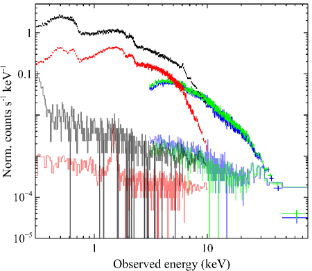
Figure 1: The time-averaged XMM-Newton and NuSTAR spectra from our coordinated 2018 observation of IRAS 09149–6206 (epoch 1). The EPIC-pn and EPIC-MOS data (XMM-Newton) are shown in black and red, while the FPMA and FPMB data (NuSTAR) are shown in green and blue, respectively. The background levels for each instrument are shown with the solid, stepped lines with slightly lighter shading than their corresponding source spectra.

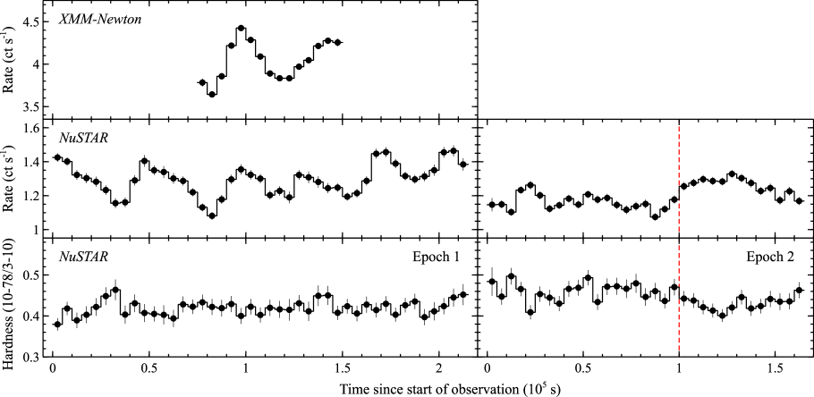
Figure 2: The X-ray lightcurves seen by XMM-Newton (0.3–10 keV, EPIC-pn; top panel) and NuSTAR (3–78 keV, FPMA+FPMB; middle panels) during the 2018 observations of IRAS 09149–6206 (5 ks bins). We also show the ratio of the 10–78 keV and 3–10 keV bands for the NuSTAR data (bottom panels). Although there is clear flux variability, there is little evidence for significant spectral variability during epoch 1, and only moderate spectral variability during epoch 2. The vertical dashed line on the right indicates the point at which we split the epoch 2 data into epochs 2a and 2b (see Section 3.2.2).

2.2 XMM-Newton

The XMM-Newton observation presented here was timed to simultaneously overlap with some portion of the first of the two NuSTAR observations. The reduction of these data was also carried out following standard procedures, using the XMM-Newton Science Analysis System (sas v18.0.0).

For the EPIC detectors, we cleaned the raw observation files using epchain and emchain for the EPIC-pn detector (Strüder et al. 2001) and the two EPIC-MOS units (Turner et al. 2001), respectively. All of the EPIC detectors were operated in Small Window mode. Source spectra and lightcurves were extracted from the cleaned eventfiles with xmmselect using a circular region of radius 35^′′. For the EPIC-pn detector, the background was estimated from a larger region of blank sky on the same detector chip as the source. For the EPIC-MOS detectors, the region of the central chip used in Small Window mode is too small to take a similar approach, so the background was estimated from large regions of blank sky on adjacent chips. The EPIC data were free of any significant background flaring, so the whole exposure was used. As recommended, we only utilized single and double patterned events for EPIC-pn (PATTERN $\leq$ 4) and single to quadruple patterned events for EPIC-MOS (PATTERN $\leq$ 12). The necessary instrumental response files for each of the detectors were generated using rmfgen and arfgen, and after performing the reduction separately for the two EPIC-MOS units we also combined these data into a single spectrum using addascaspec. Lightcurves are corrected for the PSF losses using epiclccorr. The total incident count rates ($\sim$4 $\rm\thinspace ct~{}s^{-1}$ for EPIC-pn and $\sim$1.4 $\rm\thinspace ct~{}s^{-1}$ for each EPIC-MOS unit) were sufficiently low that, given the use of the Small Window mode, pile-up is of no concern. They are also sufficiently high that the source flux is always a factor of 10 or more above the background level across the full EPIC bandpass (again, see Figure 1).

The data from the Reflection Grating Spectrometer (RGS; den Herder et al. 2001) were also reduced using rgsproc, which extracts both the spectral products and their associated instrumental response files, adopting both the standard source and background regions. As with the EPIC data, there were no periods of high background (background rate of $>$ 0.15 $\rm\thinspace ct~{}s^{-1}$) in either detector (RGS1/2) and so the full exposure was used. The net source count rates were $\sim$0.06 $\rm\thinspace ct~{}s^{-1}$ for each RGS detector, and we merged the data from the two using the rgscombine routine after confirming there were no notable differences between them over the energies where both provide coverage.

2.3 Swift

For the Swift snapshot taken with the second NuSTAR exposure, we extracted the spectrum from the XRT (Burrows et al. 2005). Cleaned event files were generated with xrtpipeline using the standard filtering, and spectral products were extracted with xselect. Source spectra were taken from a circular region of radius $\sim$45”, and as before the background was estimated from a larger, adjacent region free of contaminating point sources. The ancilliary response matrix was were generated with xrtmkarf, and we use the latest redistribution matrix available in the Swift calibration database.

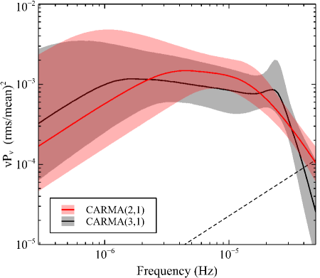
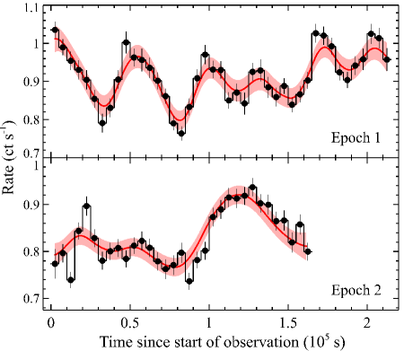
Figure 3: Left panel: the best-fit CARMA(2,1) and CARMA(3,1) models for the 3–10 keV PSD of IRAS 09149–6206 (red and black, respectively), based on the NuSTAR lightcurves. The solid lines show the best-fit PSD model in each case, the shaded regions indicate their $\pm$ 1$\sigma$ uncertainties, based on the uncertainties on the Lorentzian component parameters from the MCMC chains, and the dashed line indicates the level of the Poisson noise. Right panel: the fit to the 3–10 keV NuSTAR lightcurve provided by the CARMA(2,1) model. The black points show the data (5 ks time bins, as in Figure 2), and the solid red line and shaded area again show the best-fit model and its $\pm$ 1$\sigma$ uncertainties.

3 Analysis

3.1 Variability

We show the XMM-Newton and NuSTAR lightcurves from the 2018 observations in Figure 2. Flux variability is clearly seen from IRAS 09149–6206 during the observations presented here. In particular, one feature that catches the eye in the NuSTAR data from epoch 1 is a potential quasi-periodic oscillation (QPO) on a timescale of $\sim$40 ks. As such, we were granted the second NuSTAR exposure (epoch 2) to see if this behaviour continued, but there there is no visible indication for the same variations in these data. In order to investigate whether there are any spectral variations we also compute the hardness ratio between the 3–10 and 10–78 keV bands with the NuSTAR data. We see no significant evidence for spectral changes associated with the flux variability across epoch 1. However, during epoch 2 there is some mild variation in the hardness ratio with the source flux, with the first part of the observation (before an elapsed time of $\sim$10⁵ s) slightly fainter and slightly harder than the second part, which is broadly similar to the epoch 1 data.

In order to further characterise the variability seen from IRAS 09149–6206, particularly in light of the variations seen in epoch 1, we estimate the power spectral density (PSD) from the NuSTAR data. The sampling of the observations means there are orbital gaps related to the low-earth orbit of NuSTAR (note that these are not obvious in Figure 2 owing to the binning used) as well as a larger gap between the two pointed observations. We therefore estimated the PSD using the continuous-time autoregressive moving average (CARMA) method (Kelly et al. 2014) with the public code carma_pack. This assumes the light curve results from a Gaussian noise process and estimates the model power spectrum as the sum of multiple Lorentzian components, and is well suited to dealing with non-continuous datasets as it fits the model to the lightcurve data in the time domain. The two NuSTAR observations are modelled together in order to include the largest number of cycles for the timescale of interest (i.e. $\sim$40 ks) and to give the best constraints on the PSD at low frequencies. We considered CARMA($p$,$q$) models, where $p$ is the number of autoregressive coefficients and $q$ is the number of moving average coefficients, for a stationary process with $q<p$ (see Kelly et al. 2014 for more details). The Bayesian posterior summaries for the Lorentzian function parameters are formed using a MCMC sampler. A binsize $dt=3000$ s was used giving a total number of bins $N_{\rm bins}=126$, but we stress that the results obtained do not depend on the precise binning used.

As discussed by Moreno et al. (2019), CARMA models with $q\geq 1$ are appropriate for accreting systems. We therefore consider the two simplest models, CARMA(2,1) and CARMA(3,1) for the variability exhibited by IRAS 09149–6206, and show the resulting power spectra in Figure 3. These have a fairly typical shape for AGN: a slope of $\sim f^{-\alpha}$ with $\alpha>2$ at frequencies above a characteristic break, $\nu_{\rm b}$, below which a slope of $\alpha\sim 1$ is observed (e.g. Uttley et al. 2002; Markowitz et al. 2003; Papadakis et al. 2010; González-Martín & Vaughan 2012; Alston et al. 2019). The best-fit CARMA(2,1) and CARMA(3,1) models found here describe the PSD with a series of either two or three Lorentzians, respectively, while most prior work modelling AGN PSDs has described them with the broken powerlaw model described above. Here we assume that the centroid of the highest-frequency Lorentzian in our PSD model corresponds to the break frequency, as this is the component that contributes the power around the breaks in Figure 3 (left).

The parameters of these Lorentzians are given in Table 2. Uncertainties on the timing parameters are quoted at the 68.3% level (i.e. 1$\sigma$). The extra Lorentzian in the CARMA(3,1) model is at higher frequencies again than the highest-frequency component in the CARMA(2,1) model, and the best-fit parameters of this component are actually fairly narrow and could be considered QPO-like, with the centroid frequency corresponding to a timescale of $\sim$40 ks. This component is therefore likely driven by the variations seen in epoch 1 (as noted previously, these variations are not seen in epoch 2, although even in the rare cases where AGN QPOs have been robustly detected, they appear to be transient; Alston et al. 2014b). However, the parameters of this component are very poorly constrained, and based on the CARMA likelihood fits to the lightcurves, the addition of this third Lorentzian component is not particularly significant (the log-likelihoods are 278.0 and 280.1 for the (2,1) and (3,1) models, respectively, giving a probability of chance improvement for the more complex (3,1) model of $\sim$0.25 based on a likelihood ratio test with 3 extra free parameters). This is also the case if we consider epoch 1 by itself. Further observations will be required to determine whether the CARMA(3,1) model is genuinely a better description of the variability in IRAS 09149–6206, and if so to robustly determine whether the highest frequency component is QPO-like or not. Given this, we therefore consider the CARMA(2,1) model as our preferred solution at the current time, and adopt a break frequency of $\nu_{b}=(1.11\pm 0.55)\times 10^{-5}$ Hz, corresponding to a break timescale of $T_{b}=1.0\pm 0.5$ days. The fit to the 3–10 keV NuSTAR lightcurve provided by this model is shown in Figure 3 (right).

Table 2: Parameters for the highest-frequency Lorentzians in the best-fit CARMA(2,1) and CARMA(3,1) models for the PSD of IRAS 09149–6206. Uncertainties on the timing parameters are quoted at the 68.3% level.

PSD Model	Centroid	Width
	[$10^{-5}$ Hz]	[$10^{-5}$ Hz]
CARMA(2,1)	$1.11\pm 0.55$	$2.52^{+2.48}_{-1.64}$
CARMA(3,1)	$2.34\pm 1.35$	$0.23^{+0.23}_{-0.17}$

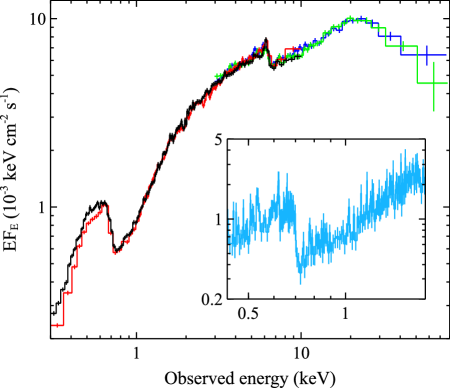
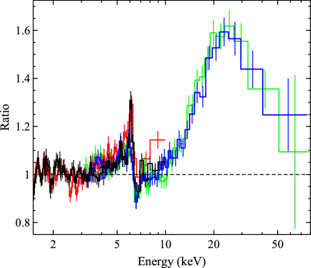
Figure 4: Left panel: the broadband XMM-Newton+NuSTAR spectrum from epoch 1, after being unfolded through a model that is constant with energy. Colours in the main panel have the same meaning as Figure 1. The data show the source to be moderately absorbed, with absorption from ionised oxygen in a warm absorber clearly seen at $\sim$0.7 keV. The inset shows the XMM-Newton RGS data in light blue, confirming the oxygen absorption. Right panel: residuals to a simple cutoffpl continuum, modified by a partially covering neutral absorber, and applied to the broadband data over the 1.5–4, 7–10 and 50–78 keV energy ranges. The key signatures of relativistic disc reflection are seen: a relativistically broadened iron line at $\sim$6 keV and a strong Compton hump at $\sim$20 keV. The data in all panels have been rebinned for visual purposes.

3.2 Spectroscopy

We now present a spectral analysis of the 2018 observations. We use XSPEC  v12.6.0f (Arnaud 1996) to model the data, and quote uncertainties on the spectral parameters at the 90% confidence level for a single parameter of interest. The broadband datasets (EPIC-pn and EPIC-MOS for XMM-Newton, FPMA and FPMB for NuSTAR) are all binned to a minimum signal to noise (S/N) of 5 per energy bin, and we fit using $\chi^{2}$ minimisation. The XMM-Newton RGS data are binned to a lower level of S/N $\geq$ 3 per bin, in order to preserve more of the spectral resolution while still being sufficient for $\chi^{2}$ minimisation (note that these S/N requirements are imposed after background subtraction). Given the relatively limited S/N of the RGS data, we focus on modelling this simultaneously with the EPIC and NuSTAR datasets in this work. We fit the EPIC data over the 0.3–10.0 keV band, the RGS data over the 0.43–1.77 keV band (7–29 Å), and the NuSTAR data over the 3–78 keV band. Throughout our analysis we allow multiplicative constants to vary between the various detectors for data from the same epoch, primarily in order to account for cross-calibration uncertainties between them. In the case of the coordinated XMM-Newton+NuSTAR observation, these constants also account for differences in the average flux level that result from the source variability (Figure 2) and the different temporal coverage of the two exopsures. We fix FPMA at unity, and the others are found to be within $\sim$15% of this value. This is similar to the level of the cross-calibration differences expected between XMM-Newton and NuSTAR (flux differences of $\sim$10%; Madsen et al. 2015), suggesting that the average flux was broadly similar across the two exposures, despite their different durations. We initially focus our spectral analysis on the coordinated XMM-Newton+NuSTAR observation (i.e. epoch 1; Section 3.2.1) before proceeding to consider the full 2018 dataset (epochs 1 and 2; Section 3.2.2).

3.2.1 The Coordinated XMM-Newton+NuSTAR Observation

Given the lack of variability seen in the hardness ratio during epoch 1 (see Figure 2), we fit these data as a single, time-averaged spectrum. This broadband spectrum is shown in Figure 4 (left panel). The source is clearly moderately absorbed, with a strong oxygen edge from O VII seen at $\sim$0.7 keV, implying that the absorbing material is partially ionised, as also concluded by Ricci et al. (2017a) based on a previous short XMM-Newton observation (and thus is not associated with the interstellar medium). Such ‘warm’ absorbers are not uncommon in the X-ray spectra of AGN (potentially seen in $>$50% of Seyfert galaxies; e.g. Reynolds 1997; Blustin et al. 2005; Laha et al. 2014).

To highlight the features at higher energies, we also show the data/model ratio of the combined XMM-Newton+NuSTAR data above 1.5 keV to a simple model consisting of a cutoffpl continuum with neutral, partially covering absorption (assumed to be at the redshift of IRAS 09149–6206) fit to the 1.5–4, 7–10 and 50–78 keV bands (here energies are given in the observed frame) where the primary AGN continuum would be expected to dominate (Figure 4, right panel). For the neutral absorber, we use tbabs (Wilms et al. 2000), adopting the cross-sections of Verner et al. (1996) and the solar abundance set of Grevesse & Sauval (1998) for self-consistency with the xillver reflection models (García & Kallman 2010) and the xstar photoionisation code (Kallman & Bautista 2001), which are used in our final, more detailed model for IRAS 09149–6206 (see below). Although the absorption is partially ionised in reality, this is only supposed to be an illustrative fit, and allowing the neutral absorber to be partially covering gives it the flexibility to account for the absorption curvature in the spectrum above $\sim$1.5 keV. We find a column density of $N_{\rm{H}}\sim 2.5\times 10^{22}$ $\rm\thinspace cm^{-2}$, a covering factor of $C_{\rm{f}}\sim 0.7$, a photon index of $\Gamma\sim 1.9$ and a cutoff energy of $E_{\rm{cut}}\sim 60$ keV. This simple model leaves strong residuals in the high-energy portion of the spectrum. Most notably, a broad emission feature is clearly seen in the iron bandpass, and a strong excess of emission is also seen above 10 keV. This high-energy excess peaks at $\sim$20–30 keV, as expected for a Compton reflection continuum. As well as these broad features, a narrower core to the iron emission at $\sim$6 keV is clearly visible (corresponding to $\sim$6.4 keV in the rest-frame of IRAS 09149–6206), and evidence for a narrow absorption feature, most likely from Fe XXV, can also be seen at $\sim$6.6 keV ($\sim$7 keV rest-frame). Such absorption is also not uncommon in other AGN (e.g. Risaliti et al. 2005; Walton et al. 2018). However, in addition to these astrophysical features, we also see evidence for residual features associated with the instrumental edges in the XMM-Newton data at $\sim$2 keV (in both EPIC-pn and EPIC-MOS). We therefore subsequently exclude the 1.7–2.5 keV energy range for these detectors for the rest of our spectral analysis.

We construct a spectral model in which the intrinsic emission from the central AGN – which consists of the primary Comptonised X-ray continuum and the associated relativistic reflection from the inner accretion disc – is absorbed by a multi-component warm absorber. We also include a neutral reflector to account for the narrow core of the iron emission, which is not subject to the warm absorber, and neutral absorption associated with our own Galaxy, which acts on all emission components. The Galactic column density towards IRAS 09149–6206 is $N_{\rm{H,Gal}}=1.58\times 10^{21}$ $\rm\thinspace cm^{-2}$ (HI4PI Collaboration et al. 2016).

Both the relativistic reflection and the primary continuum from the illuminating X-ray source are accounted for with the relxill family of models (v1.3.3; García et al. 2014). In particular, we use the relxilllp_ion_cp variant, which self-consistently treats the radial emissivity of the disc assuming a lamppost geometry (characterised by the height of the X-ray source, $h$) and assumes that the primary X-ray continuum is a thermal Comptonisation spectrum as Compton up-scattering of disc photons is generally expected to be the physical origin of this emission (e.g. Haardt & Maraschi 1991); specifically the model assumes an nthcomp continuum, characterised by the photon index, $\Gamma$, and the electron temperature, $kT_{\rm{e}}$ (Zdziarski et al. 1996; Zycki et al. 1999). Although the lamppost model assumes a specific, and simplistic geometry, it is nevertheless a useful framework as it permits a physical interpretation for the reflection fraction, $R_{\rm{frac}}$ (see Dauser et al. 2016 for the definition of $R_{\rm{frac}}$ used in the latest relxill models), and also allows non-physical regions of parameter space (e.g. a very steep radial emissivity profile and a non-rotating black hole) to be excluded. Following recent work (Svoboda et al. 2012; Kammoun et al. 2019; Ingram et al. 2019), we also allow for the possibility of an ionisation gradient across the disc, assuming this has a powerlaw form with radius (characterised by the index $p$ such that $\xi(r)\propto r^{-p}$), as this allows us to make an agnostic assessment of whether these effects are important here. We also assume that the inner accretion disc reaches the innermost stable circular orbit (ISCO) in all our analysis, and fix the outer disk to the maximum value allowed by the model (1000 $R_{\rm{G}}$, where $R_{\rm{G}}$= $GM_{\rm{BH}}/c^{2}$ is the gravitational radius), and initially we allow $R_{\rm{frac}}$ to vary as a free parameter. The other key free parameters are the inclination of the disc, its innermost ionisation parameter, and the iron abundance of the infalling material ($i$, $\xi_{\rm{in}}$ and $A_{\rm{Fe}}$, respectively; the rest of the elements included in the xillver/relxill models are assumed to have solar abundances). The ionisation parameter is defined as standard: $\xi=L_{\rm{ion}}/nR^{2}$, where $L_{\rm{ion}}$ is the ionising luminosity (integrated over the 0.1–1000 keV bandpass in relxill/xillver), $n$ is the density of the material, and $R$ is the distance to the ionising source.

The distant reflection is modelled with xillver_cp, as this also assumes an nthcomp input continuum and shares most of its key parameters with relxilllp_ion_cp. We assume that the distant reflector is nearly neutral ($\log[\xi/(\rm{erg}~{}\rm{cm}~{}\rm{s}^{-1})]$, the lowest value accepted by xillver_cp) and sees the same ionising continuum as the disc, after accounting for the gravitational redshift implied by $a^{*}$ and $h$ in the lamppost geometry (similar to Walton et al. 2019). Although xillver_cp assumes a slab geometry, which may not be appropriate for the distant reflector, Walton et al. (2018) found that similar results were obtained for the disc reflection regardless of the geometry assumed for this emission even in the more absorbed case of IRAS 13197-1627.

Lastly, we use the xstar photoionisation code (Kallman & Bautista 2001) to generate suitable grids of absorption models for the ionised absorption. We generate two different grids, with the first designed to model the lower ionisation gas that contributes the oxygen absorption, and the second designed to model the higher ionisation gas that contributes the iron absorption. Both grids allow for the ionisation parameter, column density, outflow velocity and iron and oxygen abundances as free parameters. Note that for xstar, the bandpass for the ionising luminosity is defined to be 1–1000 Ry (i.e. 13.6 eV – 13.6 keV). All other elements have solar abundances. We assume a velocity broadening of 100 $\rm\thinspace km~{}s^{-1}$ for the lower ionisation gas (a value typically assumed for such absorption; e.g. Laha et al. 2014; Longinotti et al. 2019), and a velocity broadening of 3000 $\rm\thinspace km~{}s^{-1}$ for the higher ionisation gas (also motivated by the broadening used in previous work on similar absorbers; e.g. Risaliti et al. 2005; Walton et al. 2018). We assume a fairly generic ionising continuum of $\Gamma=2$ in both cases to allow for broader applicability; this is reasonably close to the typical X-ray spectrum for unobscured AGN (Ricci et al. 2017a). For self-consistency, we link the iron abundance parameters across all the different model components associated with IRAS 09149–6206. We also link the oxygen abundances for all of the ionised absorption components (this is not currently a free parameter in the xillver/relxill models).

Table 3: Results obtained for the lamppost reflection model fit to the broadband XMM-Newton+NuSTAR data for IRAS 09149–6206. Uncertainties on the spectral parameters are quoted at the 90% level.

Component	Parameter
WA1	$\log\xi$	$\log$[erg cm s-1]	$1.12^{+0.04}_{-0.06}$
	$N_{\rm{H}}$	[$10^{22}$ cm-2]	$1.00^{+0.07}_{-0.04}$
	$A_{\rm{O}}$	[solar]	$1.24^{+0.08}_{-0.06}$
	$v_{\rm{out}}$	[$\rm\thinspace km~{}s^{-1}$]	$4200\pm 400$
	$C_{\rm{f}}$	[%]	$81^{+2}_{-3}$
WA2	$\log\xi$	$\log$[erg cm s-1]	$2.00^{+0.01}_{-0.02}$
	$N_{\rm{H}}$	[$10^{22}$ cm-2]	$6.2^{+0.2}_{-0.3}$
	$v_{\rm{out}}$	[$\rm\thinspace km~{}s^{-1}$]	$7300^{+400}_{-500}$
	$C_{\rm{f}}$	[%]	$67^{+1}_{-2}$
HIA	$\log\xi$	$\log$[erg cm s-1]	$3.44^{+0.04}_{-0.06}$
	$N_{\rm{H}}$	[$10^{22}$ cm-2]	$6.5^{+1.2}_{-1.4}$
	$v_{\rm{out}}$	[$\rm\thinspace km~{}s^{-1}$]	$9300\pm 1000$
relxill[a]	$\Gamma$		$2.16\pm 0.02$
	$kT_{\rm{e}}$[b]	[keV]	$90^{+80}_{-30}$
	$a^{*}$		$0.94^{+0.02}_{-0.06}$
	$i$	[∘]	$42^{+2}_{-1}$
	$h$	[$R_{\rm{G}}$]	$3.6^{+1.2}_{-0.5}$
	$R_{\rm{frac}}$		$2.1\pm 0.2$
	$\log\xi_{\rm{in}}$	$\log$[erg cm s-1]	$1.9\pm 0.2$
	$p$		$0.10^{+0.23}_{-0.05}$
	$A_{\rm{Fe}}$	[solar]	$1.8\pm 0.1$
	Norm	[$10^{-4}$]	$3.9^{+1.0}_{-0.3}$
xillver[a]	Norm	[$10^{-5}$]	$2.0^{+0.4}_{-0.5}$
$\chi^{2}$/DoF			3336/3201

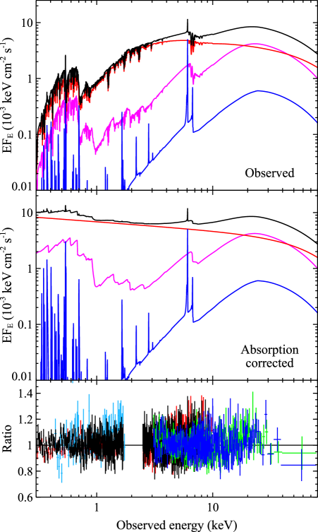
Figure 5: Top panel: the relative contributions of the different components for our broadband spectral model for the coordinated XMM-Newton+NuSTAR observation of IRAS 09149–6206 (epoch 1). The total model is shown in black, the Comptonised continuum in red, the relativistic disc reflection in magenta, and the distant reflection in blue. Middle panel: same as the top panel, but with all of the absorption components removed. Bottom panel: The data/model ratio for our broadband fit. The data have been rebinned for visual purposes, and the colours have the same meanings as in Figure 4.

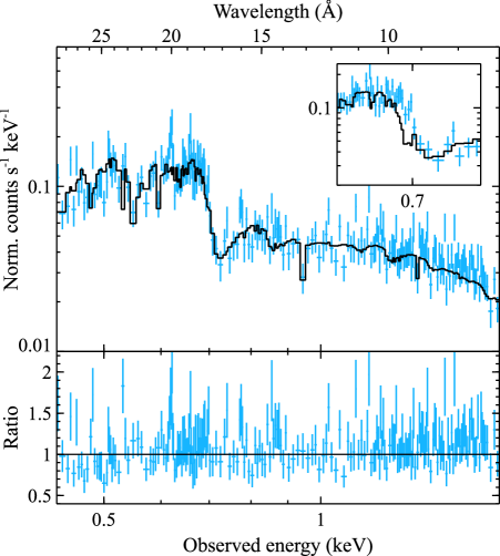
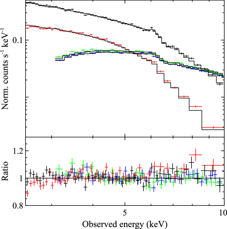
Figure 6: Zoomed in fits to the XMM-Newton RGS data (left panels) and the iron K bandpass (right panels). For each of these energy ranges we show the fits in count space (top panels), and the corresponding data/model ratios (bottom panels). In all cases, the data are shown in the same colours as Figure 4, with the same binning, and the total model is shown with the stepped black line. The inset in the top-left panel shows the result of setting the outflow velocities of the WA components to zero (while holding all other parameters constant); in this case the model clearly misses the position of the main oxygen absorption edge.

During our analysis, we allow the lower ionisation xstar absorption to be partially covering using the partcov model within XSPEC (the xstar grids themselves are not calculated to include $C_{\rm{f}}$ as a free parameter, and assume this to be unity). We also find that the low-energy oxygen absorption is best described with a combination of two xstar components with different ionisation parameters, the first (WA1) contributes the majority of the O VII absorption (0.73 keV rest-frame), and the second (WA2) contributes most of the O VIII absorption (0.87 keV rest-frame). This is more complex than the absorption model used previously by Ricci et al. (2017a), but we stress that the S/N of the XMM-Newton data used in that work is significantly lower than the S/N of the data presented here. The higher ionisation absorption (HIA) is instead assumed to be fully covering for simplicity; this component essentially only contributes the iron absorption line at $\sim$6.6 keV (observed frame), so the covering factor and the column density are fully degenerate if both are allowed to vary. We note that with this treatment of the ionised absorption, we do not find the need for any further neutral component associated with IRAS 09149–6206. Our final model expression is as follows: tbabs${}_{\rm{Gal}}\times$ $($xillver_cp + WA1 $\times$ WA2 $\times$ HIA $\times$ relxilllp_ion_cp$)$, where we note again that WA1 and WA2 are both partially covering. We stress that the removal of any of these components significantly degrades the fit (by $\Delta\chi^{2}\gtrsim 20$ per degree of freedom). Although we have assumed that the ionised absorption components do not apply to the distant reflection, we also note that making the alternative assumption (i.e. that they do) does not significantly change the quality of the fits, or result in any changes in the key model parameters of interest. We have also investigated allowing for different values of $\Gamma$ for the XMM-Newton and NuSTAR data (e.g. Cappi et al. 2016; Middei et al. 2018), which could potentially result from subtly different calibrations for the two missions. However, we find that this does not make a large difference to the fit ($\Delta\chi^{2}=14$ for one more free parameter) and does not introduce significant changes in any of the key parameters of interest, so we present the model with $\Gamma$ linked between XMM-Newton and NuSTAR.

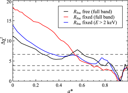
Figure 7: The $\Delta$$\chi^{2}$ confidence contours for the spin of IRAS 09149–6206 based on our spectral modeling of the coordinated XMM-Newton+NuSTAR observation (epoch 1). We show contours for our models with $R_{\rm{frac}}$ free to vary (black) and computed self-consistently from $a^{*}$ and $h$ in the lamppost geometry (red). The horizontal dotted lines represent the 90, 95 and 99% confidence levels for a single parameter of interest. We also show the contour for the latter case based on just the data above 2 keV (blue).

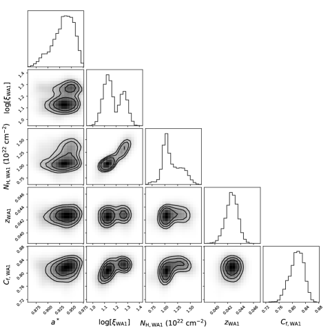
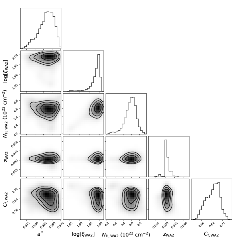
Figure 8: The MCMC results for the black hole spin vs the parameters for the two main warm absorber components (left – WA1; right – WA2) included in our model for epoch 1. Note that the outflow velocities of the absorbers are given here in terms of their redshifts in the observed frame. The 2-D contours show the 1, 2 and 3$\sigma$ confidence levels.

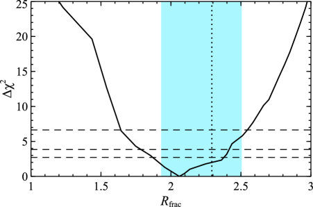
Figure 9: The $\Delta$$\chi^{2}$ confidence contours for $R_{\rm{frac}}$ when varied as a free parameter in our analysis of epoch 1 (solid black). The horizontal dotted lines represent the same confidence levels as Figure 7. The vertical dotted line indicates the predicted value of $R_{\rm{frac}}$ based on $a^{*}$ and $h$ in the lamppost geometry, and the shaded region indicates the range predicted by the 90% statistical uncertainties on these parameters.

This model describes the IRAS 09149–6206 data from epoch 1 well, with $\chi^{2}$ = 3336 for 3201 degrees of freedom (DoF), and the best-fit parameters are given in Table 3. The relative contributions of the various model components – both with and without the line-of-sight absorption – are shown in Figure 5, along with the corresponding broadband data/model ratio, showing that the model reproduces the broadband spectral shape well. We also show zoomed in fits for the XMM-Newton RGS data and the iron K bandpass in Figure 6, demonstrating the quality of fit in these key areas of the spectrum. We find that even when allowing for complex, partially covering, partially ionised absorption, the data still require a strong contribution from relativistic reflection from the innermost accretion disc. In particular, we find that the spin of the black hole is high, $a^{*}=0.94^{+0.02}_{-0.06}$, and the X-ray source is compact, $h=3.6^{+1.2}_{-0.5}$ $R_{\rm{G}}$; we show the constraints on the spin in Figure 7. One potential concern when fitting complex spectral models similar to that utilized here relates to degeneracies between different model parameters. In addition to our standard $\chi^{2}$ analysis, we therefore also perform a series of Monte Carlo Markoff Chain (MCMC) simulations to provide a further exploration of the best-fit parameter space. In particular, we make use of the MCMC functionality within XSPEC, and explore the parameter space using the Goodman-Weare algorithm (Goodman & Weare 2010) and the best-fit model as a starting point. All model parameters reported in Table 3 are free to vary throughout this analysis. We use 60 walkers, each run for 30,000 steps with a burn-in length of 5,000, resulting in a total chain of 1,500,000 parameter combinations. Chain convergence is good, with the convergence measure proposed by Geweke (1992) close to zero for every parameter. Here we focus on investigating whether there are any strong dependences between the spin parameter and the ionised absorbers in our model, since these play a major role in sculpting the observed broadband spectrum; further parameter combinations are presented in Appendix A. We find that there are no strong degeneracies between the spin and the properties of the ionised absorption components; for illustration we plot the 2-D parameter constraints from our MCMC simulations for the spin vs the key parameters for the two main warm absorber components (WA1, WA2) in Figure 8, but we stress that the same conclusion would be drawn for any of the other absorption parameters. Furthermore, the 90% uncertainty on the spin implied by these simulations is $a^{*}=0.94^{+0.02}_{-0.05}$, in excellent agreement with our $\chi^{2}$ analysis; we therefore continue with the latter in the further analysis described below.

The best-fit reflection fraction is quite large, $R_{\rm{frac}}$ = $2.1\pm 0.2$, as expected for a rapidly rotating black hole with a compact corona. In fact, the best-fit reflection fraction actually matches that predicted from the combination of $a^{*}$ and $h$ in the lamppost geometry remarkably well (predicted $R_{\rm{frac}}$ = $2.3^{+0.2}_{-0.4}$, based on the statistical constraints on $a^{*}$ and $h$; see Figure 9). We therefore re-fit the data computing $R_{\rm{frac}}$ self-consistently from $a^{*}$ and $h$; we do not report these fits in detail, since the results for the other key parameters are all consistent with those presented in Table 3, but the updated constraints on the black hole spin are also shown in Figure 7. The formal spin constraints are also similar, $a^{*}=0.91^{+0.04}_{-0.05}$, but here we find that low spin values are excluded at a much higher level of confidence. We also note that although we allow for a radial ionisation gradient, the data do not require one, as the constraints are consistent with $p=0$ in both cases; at most they only allow for a fairly shallow gradient, with $p<0.34$. This may be due to the compact nature of the corona inferred, which will in turn result in the reflected emission primarily arising from the innermost regions of the disc.

Although we find evidence that the iron abundance is mildly super-solar, we also note that the best-fit oxygen abundance for the ionised absorption is close to the solar value. As such, even though this is not a free parameter for the reflection models, there are no issues relating to significantly different abundances between the different components. The column densities and ionisation states of the absorption components are relatively typical for such warm absorbers; we show the transmission profile for each of the absorption components in Figure 10). It is worth noting that the best-fit photon index for IRAS 09149–6206 of $\Gamma\sim 2.15$ is slightly steeper than that assumed when initially calculating the xstar grids. As the definition of the ionisation parameter in xstar is based on a bandpass that extends to significantly lower energies than our X-ray data, for steeper ionising continua higher global ionisation parameters would be required to produce the same number of ionising photons in the X-ray band, and so our ionisation parameters will be systematically underestimated to some extent. To quantify this, we also calculate a small xstar grid around the best-fit parameters of the WA2 component assuming $\Gamma=2.15$ (and otherwise the same setup as described above); using this grid for WA2 instead we find that the difference in ionisation parameter is only $\Delta\log\xi\sim 0.1$. The other model parameters are all identical to the best-fit values reported in Table 3.

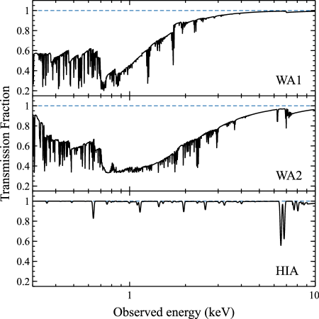
Figure 10: Transmission profiles for each of the three individual absorption components included in our spectral model for IRAS 09149–6206 (where a value of 1 indicates 100% of the incident emission is transmitted). All of the parameters for each of the individual absorbers ($\xi$, $N_{\rm H}$, $v_{\rm{out}}$, $C_{\rm{f}}$) are as quoted in Table 3. The combination of the WA1 and WA2 components dominate the oxygen absorption at low energies; WA1 contributes the majority of the O VII absorption, while WA2 contributes the majority of the O VIII absorption. The HIA component models the ionised iron absorption as a blend of Fe XXV and Fe XXVI absorption lines.

The outflow velocities found for WA1 and WA2 are relatively high for such absorption, but similar velocities have still been reported previously for outflows with similar ionisation states to those seen here (e.g. Laha et al. 2014; Longinotti et al. 2019), and forcing the WA components to have no outflow velocity clearly misses the position of the Oxygen edge (see Figure 6). We also see evidence for increasing outflow velocities with increasing ionisation parameter, potentially suggesting we are looking at radially stratified absorbers (broadly similar to that seen by Kosec et al. 2018 in emission in the narrow line Seyfert 1 1H 0707-495, albeit seen in absorption and at more modest outflow velocities here). This is in part because the data strongly prefer a solution in which the iron absorption is a blend of Fe XXV and Fe XXVI with the xstar grid used here (see Figure 10). We test this potential stratification further by repeating the fits after linking the outflow velocities of the different absorption components in various combinations. Forcing the velocity of the WA2 component to be the same as either the WA1 or HIA components (such that there are now only two distinct velocity components) only provides a mild degradation of the fit ($\Delta\chi^{2}$ =7–8 for one less free parameter in both cases), so it is plausible that WA2 could represent a distinct ionisation phase of either of these other two kinematic outflow components (e.g. Reeves et al. 2020). In both of these scenarios, the key inner disc reflection parameters remain consistent with those presented in Table 3. However, forcing all of the intrinsic absorption components (WA1, WA2, HIA) to have a common velocity does result in a significantly worse fit ($\Delta\chi^{2}=29$ for two fewer free parameters), so the data do clearly prefer at least some velocity structure to the absorption.

The best-fit absorption model predicts a variety of weak narrow features throughout the spectrum, in addition to the dominant Oxygen structure. However, these are mostly either outside of the RGS band, or the current RGS data does not have sufficient S/N to detect them individually. The only other feature associated with the ionised absorption clearly seen in the RGS data is the N VII edge (0.67 keV/18.5 Å rest-frame) seen at $\sim$0.63 keV (the edge at $\sim$0.55 keV/22.5 Å is associated with the Galactic column). There is also some mild evidence in the RGS data for a narrow emission line at 0.61 keV, which would correspond to O VIII (0.65 keV/19.1 Årest-frame) at the redshift of IRAS 09149–6206, and therefore re-emission from the WA2 component (which has the larger column of the two lower-ionisation warm absorbers). We therefore investigate including a photoionised emitter – also calculated with xstar in the same way as WA1/2 – to represent re-emission from WA2 (i.e. with the column density, ionisation parameter linked to those of WA2 and the iron and oxygen abundances linked to the rest of the model components). However, this only results in a relatively moderate improvement in the fit statistic, with $\Delta\chi^{2}=12$ for one more free parameter, and the addition of this component does not change any of the other key model parameters, so we do not include this in the final model.

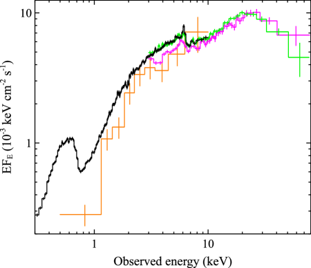
Figure 11: A comparison of the spectra of IRAS 09149–6206 from epochs 1 and 2a. For clarity, we only show the EPIC-pn, XRT and FPMA datasets, unfolded through a model that is constant with energy (as in Figure 4). For epoch 1, the colours match Figure 4, while for epoch 2a the XRT data are shown in orange, and the FPMA data in magenta. During epoch 2a, IRAS 09149–6206 exhibits a slightly harder spectrum than the rest of the data (i.e. epochs 1 and 2b, which show practically identical spectra).

3.2.2 The Combined 2018 Dataset

Having established our best-fit model for epoch 1, we now perform a combined fit including the Swift+NuSTAR data from epoch 2. As noted previously, in contrast to epoch 1 there appears to be some mild but systematic spectral variability during epoch 2, with the first part of the NuSTAR observation slightly harder than the second (see Figure 2), and the second part showing basically identical hardness to epoch 1. We therefore split the NuSTAR data, extracting separate spectra from the periods before and after an elapsed time of $T_{\rm{obs}}=10^{5}$ s. Owing to the low-earth orbit of NuSTAR, these spectra, which we refer to epochs 2a and 2b, have exposures of $\sim$72 and 44 ks, respectively. The short 1 ks Swift exposure taken along with the NuSTAR observation occurred during the first part of the observation (epoch 2a), while epoch 2b has no corresponding soft X-ray coverage. We show a comparison of the broadband spectrum from epochs 1 and 2a in Figure 11; as indicated from the simple hardness ratios shown in Figure 2, the spectrum from epoch 2a is slightly harder than epoch 1 (the spectra from epoch 2b are identical to epoch 1, also as indicated by the hardness ratios, and so are not shown for clarity).

Table 4: Results obtained for the lamppost reflection model fit to the full 2018 dataset for IRAS 09149–6206. Uncertainties on the spectral parameters are quoted at the 90% level.

Component	Parameter
Epoch 1:
WA1	$\log\xi$	$\log$[erg cm s-1]	$1.12\pm 0.05$
	$N_{\rm{H}}$	[$10^{22}$ cm-2]	$1.00^{+0.09}_{-0.08}$
	$A_{\rm{O}}$	[solar]	$1.25\pm 0.08$
	$v_{\rm{out}}$	[$\rm\thinspace km~{}s^{-1}$]	$4200^{+300}_{-400}$
	$C_{\rm{f}}$	[%]	$82^{+1}_{-2}$
WA2	$\log\xi$	$\log$[erg cm s-1]	$2.00^{+0.01}_{-0.02}$
	$N_{\rm{H}}$	[$10^{22}$ cm-2]	$6.2^{+0.2}_{-0.4}$
	$v_{\rm{out}}$	[$\rm\thinspace km~{}s^{-1}$]	$7300^{+300}_{-400}$
	$C_{\rm{f}}$	[%]	$66\pm 3$
HIA	$\log\xi$	$\log$[erg cm s-1]	$3.46\pm 0.04$
	$N_{\rm{H}}$	[$10^{22}$ cm-2]	$7.7^{+2.7}_{-1.4}$
	$v_{\rm{out}}$	[$\rm\thinspace km~{}s^{-1}$]	$9000\pm 1000$
relxill[a]	$\Gamma$		$2.16\pm 0.01$
	$kT_{\rm{e}}$[b]	[keV]	$70^{+30}_{-20}$
	$a^{*}$		$0.94^{+0.02}_{-0.07}$
	$i$	[∘]	$43^{+3}_{-2}$
	$h$	[$R_{\rm{G}}$]	$4.0^{+1.0}_{-0.3}$
	$R_{\rm{frac}}$[c]		$2.2^{+0.1}_{-0.3}$
	$\log\xi_{\rm{in}}$	$\log$[erg cm s-1]	$1.7^{+0.3}_{-0.4}$
	$p$		$<0.34$
	$A_{\rm{Fe}}$	[solar]	$1.7^{+0.2}_{-0.1}$
	Norm	[$10^{-4}$]	$3.7^{+0.2}_{-0.4}$
xillver[a]	Norm	[$10^{-5}$]	$2.0^{+0.4}_{-0.5}$
Epoch 2a: [d]
WA1	$N_{\rm{H}}$	[$10^{22}$ cm-2]	$2.5^{+0.6}_{-1.1}$
WA2	$N_{\rm{H}}$	[$10^{22}$ cm-2]	$2.0^{+2.4}_{-1.3}$
HIA	$v_{\rm{out}}$[e]	[$\rm\thinspace km~{}s^{-1}$]	$3000\pm 2000$
relxill[a]	$\Gamma$		$2.07\pm 0.02$
	Norm	[$10^{-4}$]	$2.7^{+0.2}_{-0.5}$
Epoch 2b: [d]
relxill[a]	Norm	[$10^{-4}$]	$3.5^{+0.4}_{-0.5}$
$\chi^{2}$/DoF			4749/4583

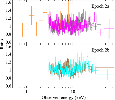
Figure 12: The data/model ratio for the data from epochs 2a and 2b with our fit to the full 2018 dataset. For epoch 2a, the XRT, FPMA and FPMB data are shown in orange, magenta and grey, respectively, matching Figure 11 (where relevant), and for epoch 2b the FPMA and FPMB data are shown in cyan and brown, respectively. The data have been rebinned for visual purposes.

We model the full 2018 dataset (epochs 1, 2a and 2b) simultaneously, with the model constructed in Section 3.2.1. For these fits, we retain the self-consistent treatment of $R_{\rm{frac}}$ in the lamppost geometry, given the results seen for epoch 1. Other key physical parameters that should not vary on observational timescales are linked across all datasets: the spin, the inclination, the iron and oxygen abundances, and the normalisation of the distant reflector. For practical purposes, given either the low S/N or lack of soft X-ray coverage available for epoch 2, we also link a variety of other parameters between the different epochs: although there is some flux variability associated with the spectral variability, this is very mild (the observed 2–10 keV flux varies by $\sim$15%), so we also link all of the various ionisation parameters across the different epochs. Furthermore, given both the lack of any soft X-ray coverage and the similarity of the NuSTAR spectra, we link all of the parameters for the warm absorber components (WA1, WA2) between epochs 1 and 2b.

Table 5: Observed fluxes for the full model and absorption-corrected fluxes for the relxill component during the 2018 observations of IRAS 09149–6206 considered here for several (rest-frame) bandpasses.

Epoch	Observed Fluxes (full model)				Absorption-Corrected Fluxes (relxill)
	[$10^{-11}$ $\rm\thinspace erg~{}cm^{-2}~{}s^{-1}$]				[$10^{-11}$ $\rm\thinspace erg~{}cm^{-2}~{}s^{-1}$]
	2–10 keV	0.3-10.0 keV	10–80 keV	0.3–80 keV	2–10 keV	0.3-10.0 keV	10–80 keV	0.3–80 keV
1	$1.54\pm 0.01$	$1.91\pm 0.02$	$2.57\pm 0.06$	$4.48^{+0.07}_{-0.06}$	$1.93\pm 0.02$	$5.0\pm 0.2$	$2.48^{+0.08}_{-0.06}$	$7.5\pm 0.2$
2a	$1.32\pm 0.02$	$1.57^{+0.07}_{-0.05}$	$2.58^{+0.08}_{-0.07}$	$4.1\pm 0.1$	$1.57\pm 0.04$	$3.7\pm 0.2$	$2.42^{+0.09}_{-0.07}$	$6.1\pm 0.2$
2b	$1.48\pm 0.02$	$1.83\pm 0.02$	$2.47\pm 0.06$	$4.30^{+0.08}_{-0.04}$	$1.85\pm 0.03$	$4.8\pm 0.2$	$2.38\pm 0.07$	$7.2\pm 0.2$

With this initial setup, we then explored which other parameters were consistent with remaining constant across the different epochs. When this occurred, we linked these parameters in our final combined fit to the data. The height of the X-ray source, the gradient of the radial ionisation profile of the accretion disc, the electron temperature of the primary continuum emission, and the column density of the HIA component were all found to be consistent with remaining constant across all epochs. The outflow velocities and the covering factors of both the warm absorber components (WA1, WA2) were consistent with remaining constant between epochs 1 and 2a (and so are effectively kept constant for all epochs). The photon indices were found to vary between epochs 1 and 2a, but were consistent for epochs 1 and 2b. Some evidence for variability in the column densities of the two warm absorber components (WA1, WA2) between epochs 1 and 2a is also seen, and the outflow velocity of the HIA component was found to vary between epochs 1 and 2 (but was consistent across epochs 2a and 2b).

The final fit to the full 2018 dataset is again very good, with $\chi^{2}$/DoF = 4749/4583. We give the constraints on the variable model parameters in Table 4; the best-fit is still extremely similar to that found for epoch 1 alone. As such, we just show the data/model ratio for the additional datasets (epochs 2a and 2b) in Figure 12. We also compute the observed and absorption-corrected fluxes for the full model and the relxill component, respectively (Table 5), to further highlight the variability accounted for by the model. For epoch 2a, the photon index is slightly harder than epochs 1 and 2b, and the column densities of the warm absorber components also show changes in the relative contributions of the two components: there is now a larger column of lower ionisation material (WA1) and a smaller column of higher ionisation material (WA2) along our line-of-sight to the central nucleus. Although there appear to be changes in both the intrinsic continuum and the line-of-sight absorption properties, the change in spectral hardness seen during epoch 2a is primarily driven by the intrinsic continuum. We note that linking the WA column densities across all epochs, such that the WA components are completely stable, only results in a mild degradation in the fit ($\Delta\chi^{2}=12$ for 2 fewer free parameters), and does not change any of the key inner disc reflection parameters of interest here (e.g. $a^{*},i$). The outflow velocity of the HIA has also decreased between epochs 1 and 2 (although this naturally has little effect on the overall hardness of the spectra). Forcing the outflow velocity to be the same for both epochs results in a significantly worse fit ($\Delta\chi^{2}=18$ for 1 less free parameter). To provide the most robust constraints we re-compute the confidence contour for the black hole spin with this joint fit, and compare these with the constraints from epoch 1 in Figure 13. The formal 90% constraints are still similar and low spin values are excluded at a much higher level of confidence than with the epoch 1 data only.

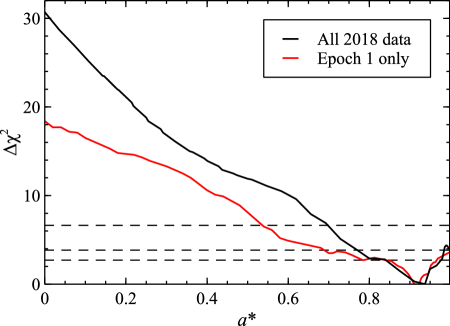
Figure 13: The $\Delta$$\chi^{2}$ confidence contours for the spin of IRAS 09149–6206 based on our spectral modeling of the full 2018 dataset with $R_{\rm{frac}}$ computed self-consistently from $a^{*}$ and $h$ in the lamppost geometry (black; see Section 3.2.2). For comparison, we also show the equivalent contour based on just the coordinated XMM-Newton+NuSTAR data (epoch 1; red, as in Figure 7). The horizontal dotted lines again represent the 90, 95 and 99% confidence levels for a single parameter of interest.

4 Discussion

We have presented a detailed analysis of the 2018 broadband X-ray observations of the type 1 Seyfert IRAS 09149–6206, combining XMM-Newton, NuSTAR and Swift. The observed X-ray spectrum is complex; the low energies are heavily influenced by a partially-ionised ‘warm’ absorber (O VII/O VIII absorption edges, as found previously by Ricci et al. 2017a), while the higher energies show clear evidence for strong relativistic reflection from the inner accretion disc (relativistically broadened iron emission and associated Compton reflection continuum, as tentatively suggested by Liebmann et al. 2018). There is also evidence for more distant reprocessing (narrow iron emission) and absorption by more highly-ionised material (Fe XXV/Fe XXVI absorption) The broadband coverage provided by XMM-Newton, NuSTAR and Swift allows us to robustly disentangle these various effects.

These data span two epochs, and flux variability is clearly observed, along with some moderate spectral variability. Although we find evidence that the properties of the warm absorber are variable to some degree, the majority of the observed variability appears to be driven by changes intrinsic to the source, and in particular the properties of the primary Comptonised X-ray continuum (i.e. $\Gamma$ and intrinsic source flux).

4.1 Black Hole Mass

The X-ray variability is characterised in Section 3.1, and we find evidence for a fairly standard AGN PSD (see Figure 3): roughly flat-topped at lower frequencies before breaking to a steep spectrum at higher frequencies (e.g. Uttley et al. 2002; Markowitz et al. 2003; Papadakis et al. 2010; González-Martín & Vaughan 2012; Alston et al. 2019). We note that the temporal separation of the two observing epochs was particularly useful in constraining the low-frequency part of the PSD here. The detection of the PSD break frequency provides us with an opportunity to constrain the mass of the black hole in IRAS 09149–6206 (McHardy et al. 2006; González-Martín & Vaughan 2012), provided the bolometric luminosity, $L_{\rm bol}$, is also known. As discussed in Section 3.1, based on our CARMA modelling of the PSD, we adopt a break timescale of $T_{\rm{b}}=1.0\pm 0.5$ days.

We estimate $L_{\rm bol}$ from the intrinsic (i.e. absorption corrected) 2–10 keV luminosities calculated for the relxill component from our spectral fits to the broadband data, utilizing the available 2–10 keV bolometric corrections in the literature ($\kappa_{2-10}\equiv L_{\rm{bol}}/L_{2-10}$). For a luminosity distance of $D=267$ Mpc (assuming a standard $\Lambda$CDM concordance cosmology, i.e. $H_{0}$ = 70 km s^-1 Mpc^-1, $\Omega_{\rm{M}}=0.3$, $\Omega_{\Lambda}=0.7$), the rest-frame 2–10 keV luminosities for epochs 1–2 are $L_{2-10}=1.6-1.9\times 10^{44}$ erg s^-1. Given the source spent more time at the higher end of this flux range during our observations, we adopt an average 2–10 keV luminosity of $L_{2-10}=1.8\times 10^{44}$ erg s^-1 for the 2018 dataset. The appropriate value of $\kappa_{2-10}$ depends on the Eddington ratio, $\lambda_{\rm{E}}\equiv L_{\rm{bol}}/L_{\rm{Edd}}$; $\kappa_{2-10}$ varies from $\sim$10 for $\lambda_{\rm{E}}\lesssim 0.01$ up to $\sim$100 for $\lambda_{\rm{E}}\sim 1$ (e.g. Vasudevan & Fabian 2009; Lusso et al. 2010). We estimate $\lambda_{\rm{E}}$ from the known correlation between $\lambda_{\rm{E}}$ and the X-ray photon index (e.g. Shemmer et al. 2008; Risaliti et al. 2009; Brightman et al. 2013). Based on the most recent of these works (Brightman et al. 2013), the values of $\Gamma$ found here ($2.07-2.16$) imply an Eddington fraction of $\lambda_{\rm{E}}\sim 0.4$. In turn, this implies a bolometric correction of $\kappa_{2-10}\sim 50$, and a bolometric luminosity of $L_{\rm{bol}}\sim 9\times 10^{45}$ erg s^-1. Given the scatter seen in $\kappa_{2-10}\sim 50$ (Lusso et al. 2010), we estimate the uncertainty on this value to be at least a factor of $\sim$2.

Combining this with the break timescale from the PSD, we estimate a black hole mass of $\log[M_{\rm{BH}}/M_{\odot}]=8.0\pm 0.6$ from the relation linking $M_{\rm{BH}}$, $L_{\rm bol}$ and $T_{\rm{b}}$ presented by McHardy et al. (2006). The final uncertainty quoted here comes from combining (in quadrature) the estimated 1$\sigma$ uncertainties on $T_{\rm{b}}$ and $L_{\rm{bol}}$ ($\sim$0.1 and $\sim$0.2 dex, respectively) with the uncertainty on the absolute mass calibration used when deriving the scaling relation (taken to be $\sim$0.4 dex; Peterson 2014). Although there is good consistency between the values for $\kappa_{2-10}$ and $L_{\rm bol}$ obtained here and the equivalent values obtained by Vasudevan et al. (2010), who estimated $L_{\rm bol}$ based on the infrared luminosity, the black hole mass obtained here is significantly smaller than the mass presented in that work, $M_{\rm{BH}}\sim 3\times 10^{9}$ $M_{\odot}$, estimated from the relation between $M_{\rm BH}$ and the $K$-band bulge luminosity (Marconi & Hunt 2003). However, as a sanity check, we note that the Eddington ratio implied by our estimated mass and bolometric luminosity is close to (but still below) unity, in reasonable agreement with that estimated from $\Gamma$ (which did not necessarily need to have been the case). Furthermore, the mass estimated here is in good agreement with that obtained by Parisi et al. (2009) based on the H$\beta$ line width, $\log[M_{\rm{BH}}/M_{\odot}]\sim 7.9$, and also with that obtained by the BASS collaboration based on the H$\alpha$ line width, $\log[M_{\rm{BH}}/M_{\odot}]\sim 8.4$ (Koss et al. 2017). We are therefore satisfied that our mass of $\log[M_{\rm{BH}}/M_{\odot}]=8.0\pm 0.6$ is robust, and provides a self-consistent solution for IRAS 09149–6206. The discrepancy with the mass reported in Vasudevan & Fabian (2009) is likely because IRAS 09149–6206 is still AGN-dominated in the $K$-band, given that it shows clear broad emission lines in the optical (Perez et al. 1989), resulting in an overestimate of the luminosity of the bulge and in turn the black hole mass.

4.2 Black Hole Spin

In addition to the mass constraint from the X-ray variability, the relativistic reflection features in the broadband X-ray spectrum allow us to measure the spin. We model this reflection self-consistently in the context of the lamppost geometry, which we find provides a very good description of the data despite being a clearly simplified geometry (e.g. Wilkins & Fabian 2012; Zhang et al. 2019), including correctly predicting the observed reflection fraction (see Figure 9). This is further support for the idea that the X-ray corona is compact and centrally located. To provide the most robust constraint on the spin, our final analysis is based on a joint fit to all of the 2018 data (epochs 1 and 2); we find that IRAS 09149–6206 hosts a rapidly rotating black hole with $a^{*}=0.94^{+0.02}_{-0.07}$ (see Figure 13). These observations have therefore allowed us to fully characterise the supermassive black hole in IRAS 09149–6206.

Systematic uncertainties on spin measurements from reflection analyses are difficult to quantify, but are likely $\Delta a^{*}\sim 0.1$ for rapidly rotating black holes with strong reflection (e.g. Bonson & Gallo 2016; Choudhury et al. 2017; Kammoun et al. 2018), i.e. similar to the statistical uncertainty in this case. We note that the models used here assume that the disc is essentially razor thin; this may be one source of systematic error, as in reality the disc is likely to have some non-negligible vertical extent. For an Eddington ratio of $\lambda_{\rm{E}}\sim 0.4$, as inferred above, the maximum scale-height of the disc should be $H/R\sim 0.15$ (McClintock et al. 2006). Significant ‘bleeding’ of the reflected emission over the ISCO is therefore unlikely (Reynolds & Fabian 2008), and we are also unlikely to have introduced significant uncertainties by assuming an emissivity profile for a thin disc (and if anything, the latter would cause us to underestimate the spin; Taylor & Reynolds 2018).

The spin constraint from this analysis comes from modelling the full suite of reflection features present in our broadband spectral model, including the relativistically broadened iron emission, the strength of the Compton reflection continuum, and the soft excess (which is partially seen through the ionised absorption; see Figure 5). Although the first two features can be readily seen in the broadband data, the presence of the ionised absorption makes it challenging to unambiguously test whether a soft excess is present in IRAS 09149–6206. Nevertheless, is seen almost ubiquitously in similar AGN that have low levels of obscuration, and its presence is implicitly assumed in the broadband reflection modelling undertaken here. However, it is important to note that the nature of the soft excess is still hotly debated. As implied here, a reflection origin is often invoked (e.g. Crummy et al. 2006; Walton et al. 2013; Jiang et al. 2019a), in which the forest of low-energy fluorescent emission lines in the rest-frame reflection spectrum are all relativistically broadened in the same way as the iron emission, and blend together to form a smooth low-energy excess. This is supported by the discovery that the soft excess exhibits the time lags relative to the primary powerlaw continuum expected in this scenario (e.g. Fabian et al. 2009, 2013; De Marco et al. 2013; Alston et al. 2014a, 2020); these lags are well explained by reverberation of the inner disc, and are similar in amplitude to the lags seen from the broad iron line (which is unambiguously associated with reflection from this region; Zoghbi et al. 2012; Kara et al. 2013, 2015). However, in some cases the reflection model does not appear to fit the broadband data well (e.g. Matt et al. 2014; Porquet et al. 2018), and an alternative model invoking distinct Comptonizing zones for the soft excess (the ‘warm’ corona) and the primary powerlaw continuum (the ‘hot’ corona) is frequently proposed as an alternative (e.g. Done et al. 2012; Petrucci et al. 2013, 2018; Middei et al. 2019; see García et al. 2019 and Petrucci et al. 2020 for the latest debate over whether such warm coronae are physically plausible). Given this, we tested how sensitive the spin constraints were to the treatment of the soft X-ray data (keeping the warm absorber components fixed at their best-fit values from the full band analysis, since these cannot be constrained with the data above 2 keV). Based on the broadband data from epoch 1, we find the constraints are practically identical when fitting the data only above 2 keV, i.e. excluding the contribution of the soft excess (see Figure 7). Our conclusion that IRAS 09149–6206 hosts a rapidly rotating black hole is therefore robust to the precise nature of the soft excess.

Throughout this work we have made use of reflection models that assume the accretion disc has a fixed electron density of $n_{\rm{e}}=10^{15}$ $\rm\thinspace cm^{-3}$. This density has been adopted as standard for the majority of the reflection models discussed in the literature (e.g. Ross et al. 1999; Ballantyne et al. 2001; Ross & Fabian 2005; García & Kallman 2010), and is motivated by the expected value for a ‘typical’ AGN, i.e. a $\sim$10⁸ $M_{\odot}$ black hole accreting at a significant fraction of its Eddington luminosity (e.g. Svensson & Zdziarski 1994). However, while it has been known for some time that this is not appropriate for the accretion discs around X-ray binaries, which should have much higher densities (e.g. Reis et al. 2009; Walton et al. 2012; King et al. 2014; Tomsick et al. 2018; Jiang et al. 2019b), more recently the density of the disc has also been shown to be an important issue even for reflection modelling within the AGN population, given the broad range of central black hole masses and accretion rates observed (García et al. 2016; Jiang et al. 2018, 2019a). Larger densities increase the rate of free-free absorption, resulting in significant changes in the reflection continuum at low energies which can be important to account for, particularly when modelling the soft excess. However, these effects can also influence the reflection continuum in the Fe K band, and thus influence the iron abundance inferred (Tomsick et al. 2018; Jiang et al. 2019a), so they are potentially important to consider in a broadband context as well. Nevertheless, the ‘typical’ AGN described above is very close to the scenario we infer for IRAS 09149–6206, so the density assumed in the models used here is actually a suitable choice, and should not introduce any significant systematic uncertainties in our spin measurement. Indeed, if we replace relxilllp_ion_cp with relxilllpd in our analysis of the XMM-Newton+NuSTAR data from epoch 1, allowing the disc density to be varied as a free parameter instead of the radial ionisation gradient (it is not currently possible to vary both simultaneously with the relxill models), we find that $\log[n_{\rm{e}}/\rm{cm}^{-3}]<15.2$. As expected, the spin constraint is essentially unchanged.

We can therefore add IRAS 09149–6206 to the growing list of rapidly rotating black holes powering radio-quiet AGN (e.g. Brenneman et al. 2011; Gallo et al. 2013; Risaliti et al. 2013; Walton et al. 2014; Marinucci et al. 2014; Svoboda et al. 2015; Buisson et al. 2018). This is further evidence that, while black hole spin may well play a significant role in powering the relativistic jets launched by accreting black holes (Blandford & Znajek 1977), the angular momentum of the black hole can not be the only ingredient necessary for jet launching (King et al. 2013). The distinction between radio-loud and radio-quiet AGN therefore cannot be simply driven by differences in spin, as has previously been suggested (e.g. Wilson & Colbert 1995; Moderski et al. 1998; Sikora et al. 2007); this would require that radio-quiet AGN host slowly rotating black holes, contrary to observation.

The high spin obtained here also has implications for the most recent period of significant growth experienced by the SMBH in IRAS 09149–6206. This likely occurred via prolonged ‘coherent’ accretion (i.e. the accreted material always has a common angular momentum axis), as this tends to produce rapidly rotating black holes, while more chaotic accretion would instead tend to spin the black hole down (e.g. Dubois et al. 2014; Sesana et al. 2014; Fiacconi et al. 2018). There is growing evidence for a ‘top-heavy’ spin distribution among local AGN (i.e. high spins are preferred; Walton et al. 2013; Reynolds 2014), which would suggest that such growth is common. However, caution is still required here, as there are known selection biases towards observing high-spin objects (Brenneman et al. 2011; Vasudevan et al. 2016) which are likely significant. Larger samples of spin measurements to overcome this bias, combined with efforts to track the redshift evolution of black hole spin (e.g. Reis et al. 2014; Reynolds et al. 2014; Walton et al. 2015) are required to properly constrain SMBH growth models in a statistical sense.

4.3 Ionised Absorption

The low-energy spectrum observed from IRAS 09149–6206 is heavily modified by the effects of absorption by partially ionised material, particularly the O VII/O VIII edges at $\sim$0.7–0.8 keV, as previously suggested by Ricci et al. (2017a). The best-fit model found here prefers two absorption components for the warm absorber: a slightly lower ionisation component with $\log[\xi/(\rm{erg}~{}\rm{cm}~{}\rm{s}^{-1})]\sim 1.1$ and a slightly higher ionisation component with $\log[\xi/(\rm{erg}~{}\rm{cm}~{}\rm{s}^{-1})]\sim 2.0$. This is more complex than the single-component absorption model used by Ricci et al. (2017a), but we stress again that this is likely related to the much lower S/N data available to them at the time. Such complexity in the warm absorber is not unusual where high S/N data is available (e.g. Lee et al. 2001; Krongold et al. 2003; Steenbrugge et al. 2005; Reeves et al. 2013). The parameters we find ($\xi$, $N_{\rm{H}}$, $v_{\rm{out}}$) are fairly typical when compared against the warm absorbers seen in other systems (e.g. Laha et al. 2014); the outflow velocities ($\sim$4000–7000 $\rm\thinspace km~{}s^{-1}$) could be considered slightly on the high side, but are not unprecedented for such absorption (e.g. Longinotti et al. 2019).

In addition to the warm absorber seen at low energies, we also see evidence for absorption from much more highly ionised material in the iron band with $\log[\xi/(\rm{erg}~{}\rm{cm}~{}\rm{s}^{-1})]\sim 3.5$ (giving Fe XXV/Fe XXVI absorption). We find this to be the fastest outflowing component in epoch 1 ($v_{\rm{out}}\sim 9000$ $\rm\thinspace km~{}s^{-1}$), although the velocity has dropped in epoch 2 ($v_{\rm{out}}\lesssim 5000$ $\rm\thinspace km~{}s^{-1}$). Qualitatively similar stratification of the various outflowing zones (higher velocity at higher ionisation) to that found in epoch 1 and velocity variability in other highly ionised outflows have both been seen previously (e.g. Kosec et al. 2018; Matzeu et al. 2017; Pinto et al. 2018). Although this component appears to reach reasonably large outflow velocities, the outflow seen here still appears to be relatively slow in comparison to the most extreme seen in other AGN (‘ultrafast’ outflows, which can reach velocities of $\sim$0.4$c$; Reeves et al. 2018; Walton et al. 2019).

Taking the observed results at face-value, and following previous work (e.g. Nardini et al. 2015; Walton et al. 2019), we attempt to estimate the kinetic power, $L_{\rm{kin}}$, of the highly ionised component relative to the bolometric radiative output via equation 1:

$$\frac{L_{\rm{kin}}}{L_{\rm{bol}}}\approx 2{\pi}m_{\rm{p}}\mu\frac{R_{\rm{w}}N_{\rm{H}}v_{\rm{out}}^{3}}{L_{\rm{bol}}}{\Omega}C_{\rm{V}}$$ (1)

where $\mu$ is the mean atomic weight $\sim$1.2 for solar abundances, $m_{\rm{p}}$ is the proton mass, $R_{\rm{w}}$ is the radius of the wind, and $\Omega$ and $C_{\rm{V}}$ are the unknown solid angle and volume filling factor of the absorber, respectively (both normalised to vary between 0–1; note that $\Omega$ is formally distinct from $C_{\rm{f}}$, which is the line-of-sight covering factor). While $R_{\rm{w}}$ is not known here, we can set a lower limit on this ratio by taking this to be the escape radius implied by the outflow velocity, i.e. $R_{\rm{w}}=R_{\rm{esc}}=GM_{\rm{BH}}/v_{\rm{out}}^{2}$. This would imply that $L_{\rm{kin}}/L_{\rm{bol}}\gtrsim 3\times 10^{-3}~{}\Omega C_{\rm{V}}$. Performing the same calculations for the WA1 and WA2 components results in even smaller values of $L_{\rm{kin}}/L_{\rm{bol}}$ (although WA2 is of the same order). Even assuming that these are all independent outflow components would therefore only increase the total $L_{\rm{kin}}/L_{\rm{bol}}$ by a factor of $\sim$2.

Simulations predict that the winds launched by accretion discs should be largely equatorial (e.g. Proga et al. 2000; Proga & Kallman 2004; Nomura et al. 2016); there is clear evidence that this is the case for X-ray binaries (Ponti et al. 2012), and there is also some evidence that AGN outflow properties are inclination dependent (Parker et al. 2018). As the inclination inferred from the reflection spectrum is fairly modest here, the true outflow velocity could yet be slightly larger owing to projection effects. However, for $i\sim 40-45$^∘ the intrinsic velocity could only be up to a factor of $\sim$1.5 larger, and $L_{\rm{kin}}$ would only increase by the same factor for $R_{\rm{w}}=R_{\rm{esc}}$ (since $R_{\rm{esc}}\propto v_{\rm{out}}^{-2}$). We also note that, given the way they have been normalised here, the product $\Omega C_{\rm{V}}$ must be $\leq 1$. Unless $R_{\rm{w}}\gg R_{\rm{esc}}$ then it is not clear the outflow seen here can be sufficient to drive galaxy-scale feedback; simulations suggest that $L_{\rm{kin}}$ must be at least a few per cent of $L_{\rm bol}$ to do so (e.g. Di Matteo et al. 2005; Hopkins & Elvis 2010). A more powerful outflow may yet be present in IRAS 09149–6206, particularly given that we infer it is accreting at close to its Eddington limit. However, if this is the case it either does not intercept our line-of-sight, which is plausible for a viewing angle of $i\sim 40-45$^∘, or is too highly ionised for a significant detection.

5 Conclusions

Combining X-ray timing and spectroscopy, we have been able to fully characterise the supermassive black hole in the type I Seyfert galaxy IRAS 09149–6206, a complex source that has received relatively little observational attention to date. We find the mass of the black hole to be $\log[M_{\rm{BH}}/M_{\odot}]=8.0\pm 0.6$ (primarily from X-ray timing constraints on the PSD break frequency provided by NuSTAR) and the spin of the black hole to be $a^{*}=0.94^{+0.02}_{-0.07}$ (from broadband X-ray spectroscopic constraints on the relativistic reflection from the inner disc, combining XMM-Newton, NuSTAR and Swift). The mass obtained here is in good agreement with that estimated previously from the H$\beta$ line width, and implies that the black hole in IRAS 09149–6206 is accreting at a reasonable fraction of its Eddington luminosity. The spin constraint presented here is the first available in the literature for IRAS 09149–6206, and shows this to be another example of a radio-quiet AGN powered by a rapidly rotating black hole.

Appendix A Further Monte Carlo Results

Here we present the results from our MCMC simulations performed for the data from epoch 1 (see Section 3.2.1) for a variety of additional parameter combinations. In Figure 14 we focus on the parameters relating to the intrinsic continuum and the disc reflection, and in Figure 15 we focus on the parameters relating to the various ionised absorbers. Note that here, the lamppost height is in units of the vertical horizon ($R_{\rm{H}}$, hence the negative values which relate to the relxill setup) which varies from $1\leq R_{\rm{H}}/R_{\rm{G}}\leq 2$, depending on the spin. In addition, outflow velocities for the absorbers are again given in terms of their redshifts in the observed frame, as in Figure 8.

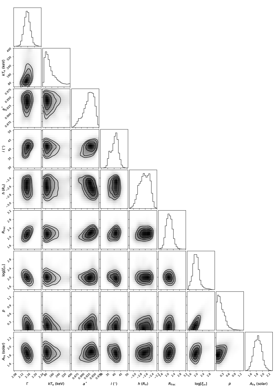
Figure 14: The MCMC results for parameters relating to the intrinsic AGN continuum and the relativistic disc reflection for the data from epoch 1. The plot format follows that of Figure 8.

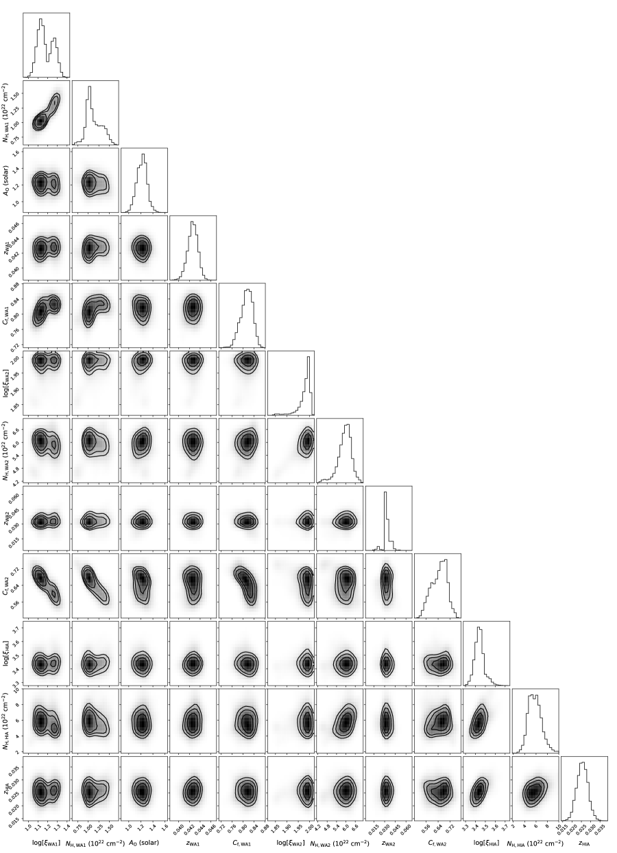
Figure 15: The MCMC results for parameters relating to the various ionised absorbers for the data from epoch 1. The plot format again follows that of Figures 8 and 14.

References

- Alston et al. (2014a) Alston W. N., Done C., Vaughan S., 2014a, MNRAS, 439, 2, 1548
- Alston et al. (2019) Alston W. N., Fabian A. C., Buisson D. J. K., et al., 2019, MNRAS, 482, 2, 2088
- Alston et al. (2020) Alston W. N., Fabian A. C., Kara E., et al., 2020, Nature Astronomy, 2
- Alston et al. (2014b) Alston W. N., Markeviciute J., Kara E., Fabian A. C., Middleton M., 2014b, MNRAS, 445, L16
- Arévalo et al. (2014) Arévalo P., Bauer F. E., Puccetti S., et al., 2014, ApJ, 791, 81
- Arnaud (1996) Arnaud K. A., 1996, in Astronomical Data Analysis Software and Systems V, edited by G. H. Jacoby & J. Barnes, vol. 101 of Astron. Soc. Pac. Conference Series, Astron. Soc. Pac., San Francisco, 17
- Ballantyne et al. (2001) Ballantyne D. R., Ross R. R., Fabian A. C., 2001, MNRAS, 327, 10
- Bauer et al. (2001) Bauer F. E., Brandt W. N., Sambruna R. M., et al., 2001, AJ, 122, 182
- Bentz et al. (2009) Bentz M. C., Walsh J. L., Barth A. J., et al., 2009, ApJ, 705, 199
- Bianchi et al. (2002) Bianchi S., Matt G., Fiore F., Fabian A. C., Iwasawa K., Nicastro F., 2002, A&A, 396, 793
- Bird et al. (2007) Bird A. J., Malizia A., Bazzano A., et al., 2007, ApJS, 170, 1, 175
- Blandford & Znajek (1977) Blandford R. D., Znajek R. L., 1977, MNRAS, 179, 433
- Blustin et al. (2005) Blustin A. J., Page M. J., Fuerst S. V., Branduardi-Raymont G., Ashton C. E., 2005, A&A, 431, 111
- Bonson & Gallo (2016) Bonson K., Gallo L. C., 2016, MNRAS, 458, 1927
- Brenneman et al. (2011) Brenneman L. W., Reynolds C. S., Nowak M. A., et al., 2011, ApJ, 736, 103
- Brightman et al. (2013) Brightman M., Silverman J. D., Mainieri V., et al., 2013, MNRAS, 433, 2485
- Buisson et al. (2018) Buisson D. J. K., Parker M. L., Kara E., et al., 2018, MNRAS, 480, 3, 3689
- Burrows et al. (2005) Burrows D. N., Hill J. E., Nousek J. A., et al., 2005, Space Science Reviews, 120, 165
- Cappi et al. (2016) Cappi M., De Marco B., Ponti G., et al., 2016, A&A, 592, A27
- Choudhury et al. (2017) Choudhury K., García J. A., Steiner J. F., Bambi C., 2017, ApJ, 851, 1, 57
- Cram et al. (1992) Cram L. E., North A., Savage A., 1992, MNRAS, 257, 602
- Crummy et al. (2006) Crummy J., Fabian A. C., Gallo L., Ross R. R., 2006, MNRAS, 365, 1067
- Dauser et al. (2016) Dauser T., García J., Walton D. J., et al., 2016, A&A, 590, A76
- De Marco et al. (2013) De Marco B., Ponti G., Cappi M., et al., 2013, MNRAS, 431, 2441
- den Herder et al. (2001) den Herder J. W., Brinkman A. C., Kahn S. M., et al., 2001, A&A, 365, L7
- Di Matteo et al. (2005) Di Matteo T., Springel V., Hernquist L., 2005, Nat, 433, 604
- Done et al. (2012) Done C., Davis S. W., Jin C., Blaes O., Ward M., 2012, MNRAS, 420, 1848
- Dubois et al. (2014) Dubois Y., Volonteri M., Silk J., 2014, MNRAS, 440, 1590
- Fabian (2012) Fabian A. C., 2012, ARA&A, 50, 455
- Fabian et al. (2013) Fabian A. C., Kara E., Walton D. J., et al., 2013, MNRAS, 429, 2917
- Fabian et al. (2009) Fabian A. C., Zoghbi A., Ross R. R., et al., 2009, Nat, 459, 540
- Ferrarese et al. (2006) Ferrarese L., Côté P., Dalla Bontà E., et al., 2006, ApJ, 644, L21
- Fiacconi et al. (2018) Fiacconi D., Sijacki D., Pringle J. E., 2018, MNRAS
- Foreman-Mackey (2016) Foreman-Mackey D., 2016, The Journal of Open Source Software, 1, 24
- Gallo & Fabian (2011) Gallo L. C., Fabian A. C., 2011, MNRAS, 418, L59
- Gallo et al. (2013) Gallo L. C., Fabian A. C., Grupe D., et al., 2013, MNRAS, 428, 1191
- García et al. (2014) García J., Dauser T., Lohfink A., et al., 2014, ApJ, 782, 76
- García & Kallman (2010) García J., Kallman T. R., 2010, ApJ, 718, 695
- García et al. (2016) García J. A., Fabian A. C., Kallman T. R., et al., 2016, MNRAS, 462, 1, 751
- García et al. (2019) García J. A., Kara E., Walton D., et al., 2019, ApJ, 871, 1, 88
- Gehrels et al. (2004) Gehrels N., Chincarini G., Giommi P., et al., 2004, ApJ, 611, 1005
- Geweke (1992) Geweke J., 1992, in Bayesian Statistics 4 (ed. J. M. Bernardo, J. O. Berger, A. P. Dawid and A. F. M. Smith), 169–193, Clarendon Press, Oxford
- González-Martín & Vaughan (2012) González-Martín O., Vaughan S., 2012, A&A, 544, A80
- Goodman & Weare (2010) Goodman J., Weare J., 2010, Communications in Applied Mathematics and Computational Science, 5, 1, 65
- GRAVITY Collaboration et al. (2020) GRAVITY Collaboration, Amorim A., Brandner W., et al., 2020, arXiv e-prints, arXiv:2009.08463
- Grevesse & Sauval (1998) Grevesse N., Sauval A. J., 1998, Space Sci. Rev., 85, 161
- Haardt & Maraschi (1991) Haardt F., Maraschi L., 1991, ApJ, 380, L51
- Harrison et al. (2013) Harrison F. A., Craig W. W., Christensen F. E., et al., 2013, ApJ, 770, 103
- HI4PI Collaboration et al. (2016) HI4PI Collaboration, Ben Bekhti N., Flöer L., et al., 2016, A&A, 594, A116
- Hlavacek-Larrondo et al. (2012) Hlavacek-Larrondo J., Fabian A. C., Edge A. C., et al., 2012, MNRAS, 421, 2, 1360
- Hopkins & Elvis (2010) Hopkins P. F., Elvis M., 2010, MNRAS, 401, 7
- Ingram et al. (2019) Ingram A., Mastroserio G., Dauser T., Hovenkamp P., van der Klis M., García J. A., 2019, MNRAS, 488, 1, 324
- Ishibashi et al. (2014) Ishibashi W., Auger M. W., Zhang D., Fabian A. C., 2014, MNRAS, 443, 2, 1339
- Ishibashi & Fabian (2015) Ishibashi W., Fabian A. C., 2015, MNRAS, 451, 1, 93
- Jansen et al. (2001) Jansen F., Lumb D., Altieri B., et al., 2001, A&A, 365, L1
- Jiang et al. (2019a) Jiang J., Fabian A. C., Dauser T., et al., 2019a, MNRAS, 489, 3, 3436
- Jiang et al. (2019b) Jiang J., Fabian A. C., Wang J., et al., 2019b, MNRAS, 484, 2, 1972
- Jiang et al. (2018) Jiang J., Parker M. L., Fabian A. C., et al., 2018, MNRAS
- Kallman & Bautista (2001) Kallman T., Bautista M., 2001, ApJS, 133, 221
- Kammoun et al. (2019) Kammoun E. S., Domček V., Svoboda J., Dovčiak M., Matt G., 2019, MNRAS, 485, 1, 239
- Kammoun et al. (2018) Kammoun E. S., Nardini E., Risaliti G., 2018, A&A, 614, A44
- Kara et al. (2013) Kara E., Fabian A. C., Cackett E. M., Uttley P., Wilkins D. R., Zoghbi A., 2013, MNRAS, 434, 1129
- Kara et al. (2015) Kara E., Zoghbi A., Marinucci A., et al., 2015, MNRAS, 446, 737
- Kaspi et al. (2000) Kaspi S., Smith P. S., Netzer H., Maoz D., Jannuzi B. T., Giveon U., 2000, ApJ, 533, 631
- Kelly et al. (2014) Kelly B. C., Becker A. C., Sobolewska M., Siemiginowska A., Uttley P., 2014, ApJ, 788, 1, 33
- King et al. (2013) King A. L., Miller J. M., Gültekin K., et al., 2013, ApJ, 771, 84
- King et al. (2014) King A. L., Walton D. J., Miller J. M., et al., 2014, ApJ, 784, L2
- Kormendy & Ho (2013) Kormendy J., Ho L. C., 2013, ARA&A, 51, 511
- Kosec et al. (2018) Kosec P., Buisson D. J. K., Parker M. L., Pinto C., Fabian A. C., Walton D. J., 2018, MNRAS, 481, 1, 947
- Koss et al. (2017) Koss M., Trakhtenbrot B., Ricci C., et al., 2017, ApJ, 850, 1, 74
- Krongold et al. (2003) Krongold Y., Nicastro F., Brickhouse N. S., Elvis M., Liedahl D. A., Mathur S., 2003, ApJ, 597, 2, 832
- Laha et al. (2014) Laha S., Guainazzi M., Dewangan G. C., Chakravorty S., Kembhavi A. K., 2014, MNRAS, 441, 3, 2613
- Lee et al. (2001) Lee J. C., Ogle P. M., Canizares C. R., et al., 2001, ApJ, 554, L13
- Liebmann et al. (2018) Liebmann A. C., Fabian A. C., Tsuruta S., Haba Y., Kunieda H., 2018, ApJ, 868, 1, 11
- Longinotti et al. (2019) Longinotti A. L., Kriss G., Krongold Y., et al., 2019, ApJ, 875, 2, 150
- Lusso et al. (2010) Lusso E., Comastri A., Vignali C., et al., 2010, A&A, 512, A34
- Lynden-Bell (1969) Lynden-Bell D., 1969, Nat, 223, 5207, 690
- Madsen et al. (2015) Madsen K. K., Harrison F. A., Markwardt C. B., et al., 2015, ApJS, 220, 8
- Malizia et al. (2007) Malizia A., Landi R., Bassani L., et al., 2007, ApJ, 668, 1, 81
- Marconi & Hunt (2003) Marconi A., Hunt L. K., 2003, ApJ, 589, 1, L21
- Marinucci et al. (2014) Marinucci A., Matt G., Miniutti G., et al., 2014, ArXiv 1404.3561
- Markowitz et al. (2003) Markowitz A., Edelson R., Vaughan S., et al., 2003, ApJ, 593, 1, 96
- Matt et al. (1996) Matt G., Fiore F., Perola G. C., et al., 1996, MNRAS, 281, 4, L69
- Matt et al. (2014) Matt G., Marinucci A., Guainazzi M., et al., 2014, MNRAS, 439, 3, 3016
- Matzeu et al. (2017) Matzeu G. A., Reeves J. N., Braito V., et al., 2017, MNRAS, 472, L15
- McClintock et al. (2006) McClintock J. E., Shafee R., Narayan R., Remillard R. A., Davis S. W., Li L.-X., 2006, ApJ, 652, 518
- McHardy et al. (2006) McHardy I. M., Koerding E., Knigge C., Uttley P., Fender R. P., 2006, Nat, 444, 730
- Middei et al. (2018) Middei R., Bianchi S., Cappi M., et al., 2018, A&A, 615, A163
- Middei et al. (2019) Middei R., Bianchi S., Petrucci P. O., et al., 2019, MNRAS, 483, 4, 4695
- Moderski et al. (1998) Moderski R., Sikora M., Lasota J.-P., 1998, MNRAS, 301, 142
- Moreno et al. (2019) Moreno J., Vogeley M. S., Richards G. T., Yu W., 2019, PASP, 131, 1000, 063001
- Nardini et al. (2015) Nardini E., Reeves J. N., Gofford J., et al., 2015, Science, 347, 860
- Nomura et al. (2016) Nomura M., Ohsuga K., Takahashi H. R., Wada K., Yoshida T., 2016, PASJ, 68, 1, 16
- Papadakis et al. (2010) Papadakis I. E., Brinkmann W., Gliozzi M., Raeth C., 2010, A&A, 518, A28
- Parisi et al. (2009) Parisi P., Masetti N., Jiménez-Bailón E., et al., 2009, A&A, 507, 3, 1345
- Parker et al. (2018) Parker M. L., Buisson D. J. K., Jiang J., et al., 2018, MNRAS
- Parker et al. (2017) Parker M. L., Pinto C., Fabian A. C., et al., 2017, Nat, 543, 83
- Perez et al. (1989) Perez E., Manchado A., Pottasch S. R., Garcia-Lario P., 1989, A&A, 215, 262
- Peterson (2014) Peterson B. M., 2014, Space Sci. Rev., 183, 1-4, 253
- Peterson et al. (2004) Peterson B. M., Ferrarese L., Gilbert K. M., et al., 2004, ApJ, 613, 2, 682
- Petrucci et al. (2020) Petrucci P. O., Gronkiewicz D., Rozanska A., et al., 2020, A&A, 634, A85
- Petrucci et al. (2013) Petrucci P. O., Paltani S., Malzac J., et al., 2013, A&A, 549, A73
- Petrucci et al. (2018) Petrucci P. O., Ursini F., De Rosa A., et al., 2018, A&A, 611, A59
- Pinto et al. (2018) Pinto C., Alston W., Parker M. L., et al., 2018, MNRAS, 476, 1021
- Ponti et al. (2012) Ponti G., Fender R. P., Begelman M. C., Dunn R. J. H., Neilsen J., Coriat M., 2012, MNRAS, 422, L11
- Porquet et al. (2018) Porquet D., Reeves J. N., Matt G., et al., 2018, A&A, 609, A42
- Pounds et al. (2003) Pounds K. A., Reeves J. N., King A. R., Page K. L., O’Brien P. T., Turner M. J. L., 2003, MNRAS, 345, 705
- Proga & Kallman (2004) Proga D., Kallman T. R., 2004, ApJ, 616, 688
- Proga et al. (2000) Proga D., Stone J. M., Kallman T. R., 2000, ApJ, 543, 686
- Qiu et al. (2019) Qiu Y., Soria R., Wang S., et al., 2019, ApJ, 877, 1, 57
- Reeves et al. (2020) Reeves J. N., Braito V., Chartas G., Hamann F., Laha S., Nardini E., 2020, ApJ, 895, 1, 37
- Reeves et al. (2018) Reeves J. N., Braito V., Nardini E., Lobban A. P., Matzeu G. A., Costa M. T., 2018, ApJ, 854, L8
- Reeves et al. (2013) Reeves J. N., Porquet D., Braito V., et al., 2013, ApJ, 776, 2, 99
- Reis et al. (2009) Reis R. C., Fabian A. C., Ross R. R., Miller J. M., 2009, MNRAS, 395, 1257
- Reis et al. (2014) Reis R. C., Reynolds M. T., Miller J. M., Walton D. J., 2014, Nat, 507, 207
- Reynolds (1997) Reynolds C. S., 1997, MNRAS, 286, 3, 513
- Reynolds (2014) Reynolds C. S., 2014, Space Sci. Rev., 183, 277
- Reynolds & Fabian (2008) Reynolds C. S., Fabian A. C., 2008, ApJ, 675, 1048
- Reynolds et al. (2014) Reynolds M. T., Walton D. J., Miller J. M., Reis R. C., 2014, ApJ, 792, L19
- Ricci et al. (2017a) Ricci C., Trakhtenbrot B., Koss M. J., et al., 2017a, ApJS, 233, 2, 17
- Ricci et al. (2017b) Ricci C., Trakhtenbrot B., Koss M. J., et al., 2017b, Nat, 549, 7673, 488
- Risaliti et al. (2005) Risaliti G., Bianchi S., Matt G., et al., 2005, ApJ, 630, L129
- Risaliti et al. (2013) Risaliti G., Harrison F. A., Madsen K. K., et al., 2013, Nat, 494, 449
- Risaliti et al. (2009) Risaliti G., Young M., Elvis M., 2009, ApJ, 700, L6
- Ross & Fabian (2005) Ross R. R., Fabian A. C., 2005, MNRAS, 358, 211
- Ross et al. (1999) Ross R. R., Fabian A. C., Young A. J., 1999, MNRAS, 306, 461
- Sesana et al. (2014) Sesana A., Barausse E., Dotti M., Rossi E. M., 2014, ApJ, 794, 104
- Shemmer et al. (2008) Shemmer O., Brandt W. N., Netzer H., Maiolino R., Kaspi S., 2008, ApJ, 682, 1, 81
- Sikora et al. (2007) Sikora M., Stawarz Ł., Lasota J.-P., 2007, ApJ, 658, 2, 815
- Steenbrugge et al. (2005) Steenbrugge K. C., Kaastra J. S., Crenshaw D. M., et al., 2005, A&A, 434, 2, 569
- Strüder et al. (2001) Strüder L., Briel U., Dennerl K., et al., 2001, A&A, 365, L18
- Svensson & Zdziarski (1994) Svensson R., Zdziarski A. A., 1994, ApJ, 436, 599
- Svoboda et al. (2015) Svoboda J., Beuchert T., Guainazzi M., Longinotti A. L., Piconcelli E., Wilms J., 2015, A&A, 578, A96
- Svoboda et al. (2012) Svoboda J., Dovčiak M., Goosmann R. W., et al., 2012, A&A, 545, A106
- Taylor & Reynolds (2018) Taylor C., Reynolds C. S., 2018, ApJ, 855, 120
- Tombesi et al. (2010) Tombesi F., Cappi M., Reeves J. N., et al., 2010, A&A, 521, A57
- Tomsick et al. (2018) Tomsick J. A., Parker M. L., García J. A., et al., 2018, ApJ, 855, 3
- Tueller et al. (2008) Tueller J., Mushotzky R. F., Barthelmy S., et al., 2008, ApJ, 681, 1, 113
- Turner et al. (2001) Turner M. J. L., Abbey A., Arnaud M., et al., 2001, A&A, 365, L27
- Uttley et al. (2002) Uttley P., McHardy I. M., Papadakis I. E., 2002, MNRAS, 332, 1, 231
- Vasudevan & Fabian (2009) Vasudevan R. V., Fabian A. C., 2009, MNRAS, 392, 1124
- Vasudevan et al. (2010) Vasudevan R. V., Fabian A. C., Gandhi P., Winter L. M., Mushotzky R. F., 2010, MNRAS, 402, 1081
- Vasudevan et al. (2016) Vasudevan R. V., Fabian A. C., Reynolds C. S., Aird J., Dauser T., Gallo L. C., 2016, MNRAS, 458, 2012
- Verner et al. (1996) Verner D. A., Ferland G. J., Korista K. T., Yakovlev D. G., 1996, ApJ, 465, 487
- Walton et al. (2018) Walton D. J., Brightman M., Risaliti G., et al., 2018, MNRAS, 473, 4377
- Walton et al. (2013) Walton D. J., Nardini E., Fabian A. C., Gallo L. C., Reis R. C., 2013, MNRAS, 428, 2901
- Walton et al. (2019) Walton D. J., Nardini E., Gallo L. C., et al., 2019, MNRAS, 484, 2544
- Walton et al. (2012) Walton D. J., Reis R. C., Cackett E. M., Fabian A. C., Miller J. M., 2012, MNRAS, 422, 2510
- Walton et al. (2015) Walton D. J., Reynolds M. T., Miller J. M., Reis R. C., Stern D., Harrison F. A., 2015, ApJ, 805, 161
- Walton et al. (2014) Walton D. J., Risaliti G., Harrison F. A., et al., 2014, ApJ, 788, 76
- Walton et al. (2016) Walton D. J., Tomsick J. A., Madsen K. K., et al., 2016, ApJ, 826, 87
- Wilkins & Fabian (2012) Wilkins D. R., Fabian A. C., 2012, MNRAS, 424, 1284
- Wilms et al. (2000) Wilms J., Allen A., McCray R., 2000, ApJ, 542, 914
- Wilson & Colbert (1995) Wilson A. S., Colbert E. J. M., 1995, ApJ, 438, 62
- Winkler et al. (2003) Winkler C., Courvoisier T. J. L., Di Cocco G., et al., 2003, A&A, 411, L1
- Winter et al. (2009) Winter L. M., Mushotzky R. F., Reynolds C. S., Tueller J., 2009, ApJ, 690, 1322
- Zdziarski et al. (1996) Zdziarski A. A., Johnson W. N., Magdziarz P., 1996, MNRAS, 283, 193
- Zhang et al. (2019) Zhang W., Dovčiak M., Bursa M., 2019, ApJ, 875, 2, 148
- Zoghbi et al. (2012) Zoghbi A., Fabian A. C., Reynolds C. S., Cackett E. M., 2012, MNRAS, 422, 129
- Zycki et al. (1999) Zycki P. T., Done C., Smith D. A., 1999, MNRAS, 309, 561