Defect Dynamics in Active Polar Fluids vs. Active Nematics

Abstract

Topological defects play a key role in two-dimensional active nematics, and a transient role in two-dimensional active polar fluids. In this paper, we study both the transient and long-time behavior of defects in two-dimensional active polar fluids in the limit of strong order and overdamped, compressible flow, and compare the defect dynamics with the corresponding active nematics model studied recently. One result is non-central interactions between defect pairs for active polar fluids, and by extending our analysis to allow orientation dynamics of defects, we find that the orientation of $+1$ defects, unlike that of $\pm 1/2$ defects in active nematics, is not locked to defect positions and relaxes to asters. Moreover, using a scaling argument, we explain the transient feature of active polar defects and show that in the steady state, active polar fluids are either devoid of defects or consist of a single aster. We argue that for contractile (extensile) active nematic systems, $+1$ vortices (asters) should emerge as bound states of a pair of $+1/2$ defects, which has been recently observed. Moreover, unlike the polar case, we show that for active nematics, a linear chain of equally spaced bound states of pairs of $+1/2$ defects can screen the activity term. A common feature in both models is the appearance of $+1$ defects (elementary in polar and composite in nematic) in the steady state.

I Introduction

In the context of biological systems, topological defects are ubiquitous, where they have been associated with cell extrusion Saw et al. (2017); Kawaguchi et al. (2017), changes in cell density Copenhagen et al. (2020) and morphogenetic processes Maroudas-Sacks et al. (2020), among others. Here we will study defects in the context of active systems, which are composed of self-propelled active units that move and exert forces on their surrounding by consuming energy, either internal or external Marchetti et al. (2013); Aditi Simha and Ramaswamy (2002). One class of active matter is active nematics, which consists of head-tail symmetric active units that tend to align, locally generating nematic (apolar) order  Ramaswamy et al. (2003); Doostmohammadi et al. (2018). For sufficiently large activity, there is a proliferation of topological defects in the nematic texture Giomi et al. (2013); Thampi et al. (2013); Giomi (2015); Doostmohammadi et al. (2017, 2018), and understanding of the dynamics of topological defects has been advanced by treating the defects as quasiparticles Keber et al. (2014); Narayan et al. (2007); Giomi et al. (2013); Pismen (2013); Shankar et al. (2018); Shankar and Marchetti (2019); Vafa et al. (2020); Zhang et al. (2020).

Another class of active matter is active polar fluids, which consists of active polar units that tend to align, locally generating polar order Ramaswamy (2010); Marchetti et al. (2013); Chaté (2020). The phase diagram of active polar fluids has been extensively studied (for example,  Kung et al. (2006); Giomi et al. (2010); Giomi and Marchetti (2012); Gopinath et al. (2012); Gowrishankar and Rao (2016); Chen et al. (2016); Chaté (2020)), and defects have been observed in for example Dombrowski et al. (2004); Riedel et al. (2005); Sokolov et al. (2007); Wensink et al. (2012); Schaller and Bausch (2013). In contrast to active nematics, since active polar fluids have long range order Toner and Tu (1995, 1998), defects are not spontaneously generated, and if generated due to boundary effect for example, the defects are expected to be transient Husain and Rao (2017); Mahault et al. (2018); Chaté (2020). That being said, aspects of dynamics of defects in active polar fluids have been studied in Kruse et al. (2004, 2005); Elgeti et al. (2011); Gopinath et al. (2012); Schaller and Bausch (2013); Gowrishankar and Rao (2016); Husain and Rao (2017). Here we study transient dynamics of defects, and give another perspective why they are transient. Applying the same argument to active nematics uncovers a 1D chain of $+1$ defects which screens the activity.

In this paper, we study both the transient and long-time behavior of defects in two-dimensional active polar fluids in the limit of strong order and overdamped, compressible flow. As in Zhang et al. (2020); Vafa et al. (2020), we consider an approximation for the global texture motivated from the passive case where the defects are widely separated and quasi-static, and use the variational principle to find defect dynamics within this ansatz. Here I shall follow the general approach of Vafa et al. (2020). In contrast to previous work on the active nematics model Narayan et al. (2007); Sanchez et al. (2012); Giomi et al. (2013); Pismen (2013); Vafa et al. (2020), in this model we find that there are no active self-propulsion terms for the lowest charge ($\pm 1$) energy excitations. Also in contrast to Vafa et al. (2020), we obtain interactions between two defects that are neither central nor perpendicular to a central force; they are generically non-central. By extending this ansatz to allow orientation dynamics of defects, we find that the orientation of $+1$ defects, unlike that of $\pm 1/2$ defects in active nematics Vafa et al. (2020), is not locked to defect positions and relaxes to asters, which we confirm with simulations. Moreover, using a scaling argument, we explain the transient feature of active polar defects and show that in the steady state, active polar fluids are either devoid of defects or consist of a single aster. We argue that for contractile (extensile) active nematic systems, $+1$ vortices (asters) should emerge as bound states of a pair of $+1/2$ defects, which has been studied in Duclos et al. (2017); Shankar et al. (2018); Kumar et al. (2018); Turiv et al. (2020); Thijssen et al. (2020); Pearce et al. (2020); Thijssen and Doostmohammadi (2020). Moreover, unlike the polar case, we show that for active nematics, a linear chain of equally spaced bound states of two $+1/2$ defects can screen the activity term. This hints at the existence of stationary lattice of bound states of pairs of $+1/2$ defects in the long term behavior of active nematics, perhaps similar to Oza and Dunkel (2016); Thijssen et al. (2020). A common feature in both models is the appearance of +1 defects (elementary in polar and composite in nematic) in the steady state.

The paper is organized as follows. We introduce the model in Sec. II and in Sec. III we review the class of quasi-stationary multi-defect solutions we use to parameterize the dynamics of textures. In Sec. IV we review the derivation of defect dynamics equations and present our results for the active induced pair-wise interactions. In Sec. V we extend our method to study orientation dynamics of defects, and in Sec. VI we offer an explanation as to why defects are transient and describe the long-time behavior. Finally, in Sec. VII we compare this model to the active nematics model introduced recently in Vafa et al. (2020). Most of the technical details are relegated to Appendices A-C.

II The Model

We consider a two-dimensional polar fluid with density $\rho$ and vector order parameter $\bf p$ described by the free energy De Gennes and Prost (1993); Kung et al. (2006) ${\mathcal{F}}(\{{\bf p}\})$:

$$\mathcal{F}(\{{\bf p}\})=\mathcal{F}_{n}(\{{\bf p}\})+\mathcal{F}_{p}(\{{\bf p}\})\;,$$ (1)

where

$${\mathcal{F}}_{n}(\{{\bf p}\})=\frac{1}{2}\int dxdy\left[C\left(\frac{\delta\rho}{\rho_{0}}\right)^{2}+K\ Tr({\nabla}{\bf p})^{2}+g(1-{\bf p}^{2})^{2}\right]\;,$$ (2)

$$\mathcal{F}_{p}(\{{\bf p}\})=\int dxdyB\frac{\rho}{\rho_{0}}\nabla\cdot\bf p$$ (3)

and $\rho_{0}$ is the equilibrium value of $\rho$.

The first term, ${\mathcal{F}}_{n}(\{{\bf p}\})$, is the usual free energy of a liquid crystal which contains only terms even in $\bf p$ De Gennes and Prost (1993), and the second term, $\mathcal{F}_{p}(\{{\bf p}\})$, contains additional terms that break this $\bf p\to-\bf p$ symmetry. $K$ is the Frank constant in the one-constant approximation, and $g$ controls the strength of polar order. We assume to be deep in the ordered state ($g\rightarrow\infty$), where the coherence length $\xi=\sqrt{K/2g}$ is the smallest relevant lengthscale and $|\vec{p}|\approx 1$ except within polar defect cores of size $a\sim\xi$. Although symmetry allows us to write terms that are odd in $\bf p$ as in $\mathcal{F}_{p}$, and that density fluctuations are generally important for polar fluids, for simplicity of analysis and in order to connect with a nematic we will assume that this contribution due to $\mathcal{F}_{p}(\{{\bf p}\})$ can be ignored, for example by imposing $\bf p\to-\bf p$ symmetry, or assuming that $b$ is small, or we are in a region where gradients in density are small.

Relaxation towards the minimum of the free energy while advection by flow $\mathbf{v}$ leads to

$$\partial_{t}p_{i}+{\bf v}\cdot\nabla{p}_{i}+\omega_{ij}p_{j}=-\frac{D}{4K}\frac{\delta{\mathcal{F}}}{\delta{p}_{i}}\;,$$ (4)

where $D$ is the diffusivity and $\omega_{ij}=(\partial_{i}v_{j}-\partial_{j}v_{i})/2$ is the vorticity. In the overdamped limit, $\mathbf{v}=v_{0}\mathbf{p}$, where $v_{0}$ has the dimensions of a speed and represents the speed of an isolated active particle. With this assumption, our equations now take the form of the Toner-Tu equations Toner and Tu (1995, 1998); Toner et al. (2005) (see Souslov et al. (2017) for a clear exposition):

$$\partial_{t}p_{i}+\frac{v_{0}}{2}{\bf p}\cdot\nabla{p}_{i}=-\frac{D}{4K}\frac{\delta{\mathcal{F}}}{\delta{p}_{i}}\;,$$ (5)

In Eq. (4) we have dropped the rate of strain alignment term Kung et al. (2006); Ramaswamy (2010) because in $2D$ and in the overdamped limit, its effect on dynamics can be represented by renormalizing the advection term. We rescale length with $\ell$, where $\ell$ is the characteristic separation between topological defects, and time with $\tau=\ell^{2}/D$. We assume that defects are widely separated, that is $\ell\gg\xi$, and thus define the dimensionless small parameter $\epsilon=\xi/\ell\ll 1$. We also define the dimensionless activity parameter $\lambda=v_{0}/8D$.

As in Vafa et al. (2020), it is convenient to adopt the language of complex analysis. In terms of complex coordinates $z=x+iy$ and ̵̄$\bar{z}=x-iy$, the complex partial derivatives $\partial=\partial_{z}=\frac{1}{2}(\partial_{x}-i\partial_{y})$ and ${\bar{\partial}}=\partial_{\bar{z}}=\frac{1}{2}(\partial_{x}+i\partial_{y})$, and the complex order parameter $p=p_{x}+ip_{y}$, the (dimensionless) free energy takes the form

$${\mathcal{F}}(\{p\})=\int dzd{\bar{z}}\left[4|\partial p|^{2}+\epsilon^{-2}(1-|p|^{2})^{2}\right]\;.$$ (6)

Finally, the equation of motion can be written as

$$\partial_{t}p=\mathcal{I}(p)=-\frac{\delta{\mathcal{F}}(\{p\})}{\delta{\bar{p}}}+\lambda\mathcal{I}_{\lambda}(p)\;,$$ (7)

where

$$\mathcal{I}_{\lambda}(p)=-(p\partial+\bar{p}\bar{\partial})p\;.$$ (8)

III Stationary and quasi-stationary textures deep in the ordered state

For simplicity, we first consider the passive case where $\lambda=0$. Then we are interested in solving

$$\partial_{t}p=-\frac{\delta{\mathcal{F}}(\{p\})}{\delta{\bar{p}}}=4\partial\bar{\partial}p+2\epsilon^{-2}(1-|p|^{2})\;.$$ (9)

Since this model was studied in Vafa et al. (2020), we will simply review it here. The single defect solution is

$$p=\psi(z,{\bar{z}})=A(|z|)\left(\frac{z}{|z|}\right)^{\sigma}\;,$$ (10)

with the amplitude $A(|z|)$ describing the defect core Pismen (1999): as $r\to 0$, $A(r)\propto r$, and for $r\gg\epsilon$, $A(r)\simeq 1-\frac{\epsilon^{2}}{4r^{2}}$ (see Appendix A for more details about $A$).

The multi-defect solution takes the form

$$p_{0}(z,{\bar{z}}|\{z_{i}\})=e^{i\psi}\prod_{i}\Psi_{i}=e^{i\psi}\prod_{i}A(|z-z_{i}|)\left(\frac{z-z_{i}}{|\bar{z}-\bar{z}_{i}|}\right)^{\sigma_{i}}\;,$$ (11)

where $\psi$ is the phase of $p$ at infinity. This texture satisfies the boundary condition $p\rightarrow e^{i\psi}e^{i\varphi\sum_{i}\sigma_{i}}$ as $|z|\rightarrow\infty$, where $\varphi$ is the polar angle. In the special case of a charge neutral system, $\sum_{i}\sigma_{i}=0$, and so $p$ is constant on the boundary.

In the limit $\epsilon\to 0$, the multi-defect texture $p_{0}(z,{\bar{z}}|\{z_{i}\})$ is the minimizer of ${\mathcal{F}}(p)$ when defects are pinned (see e.g. Pacard and Rivière (2000) and references within). In terms of the defect positions $z_{i}$, the free energy ${\mathcal{F}}_{0}={\mathcal{F}}(p_{0})$ takes the well-known form

$${\mathcal{F}}_{0}\approx 2\pi\sum_{i\neq j}\sigma_{i}\sigma_{j}\log\frac{|z_{j}-z_{i}|}{L},$$ (12)

which describes a Coulomb interaction between defect charges Chaikin and Lubensky (2000), where $L$ is the system size. Due to the Coulomb interaction, even in the absence of any “activity”, the defect cores will move to minimize the free energy ${\mathcal{F}}_{0}$. Thus even though $p_{0}$ textures minimize the free energy when defects are pinned, they are only quasi-static when the defects are no longer pinned.

As noted in Vafa et al. (2020), near a defect $z_{i}$, we can write

$$p_{0}(z,{\bar{z}})\approx P_{i}\Psi_{i}(z-z_{i},{\bar{z}}-{\bar{z}}_{i})\;.$$ (13)

where

$$P_{i}=e^{i\phi_{i}}=e^{i\psi}\prod_{j\neq i}\left(\frac{z_{i}-z_{j}}{|z-z_{j}|}\right)^{\sigma_{j}}\;.$$ (14)

is a phase factor that will play an important role in the active induced dynamics of the defects. See Fig. 1 for a geometrical interpretation.

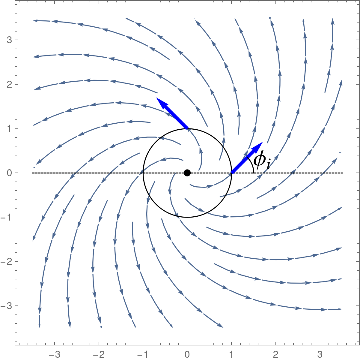
(a) $+1$ defect

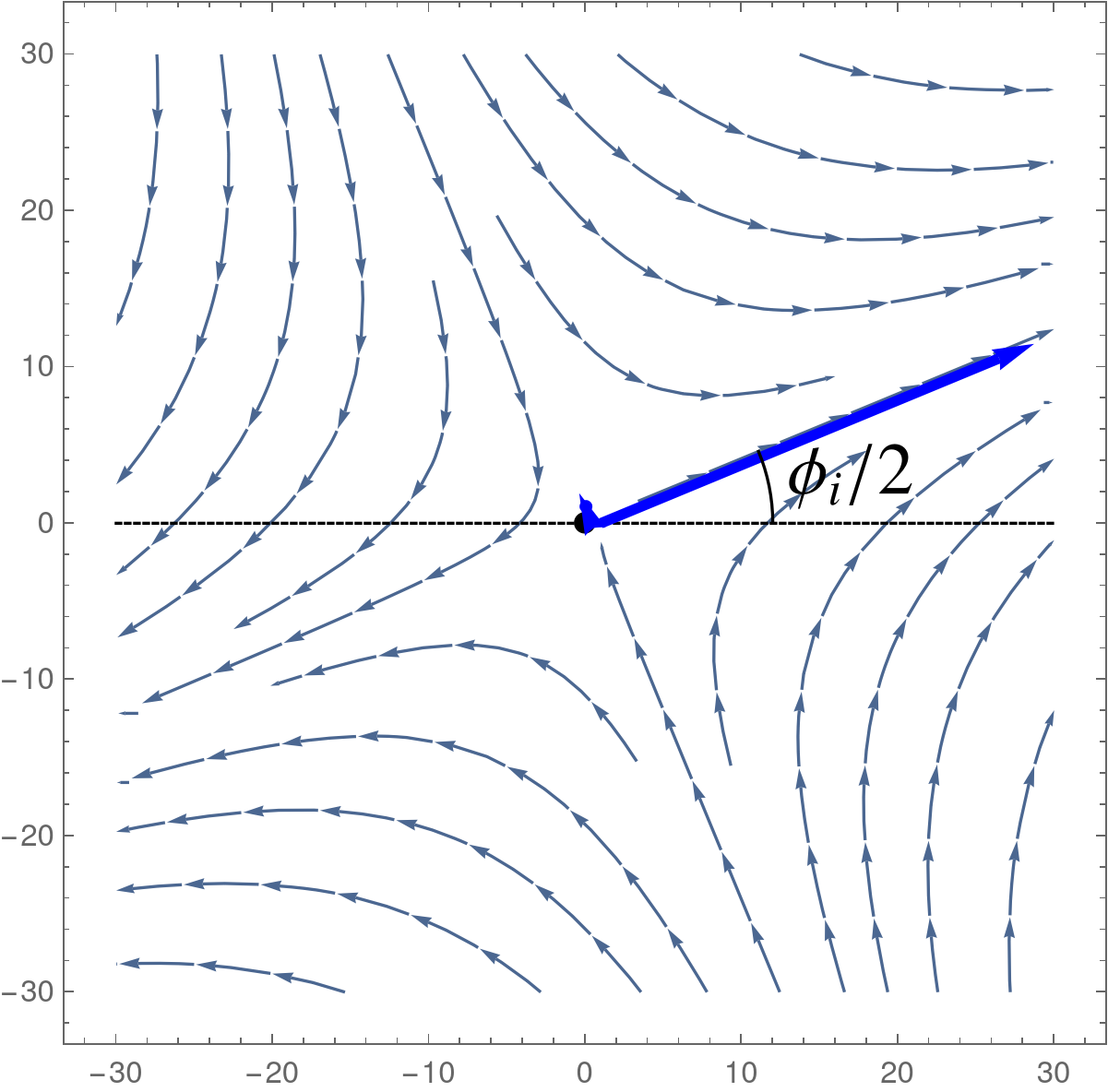
(b) $-1$ defect

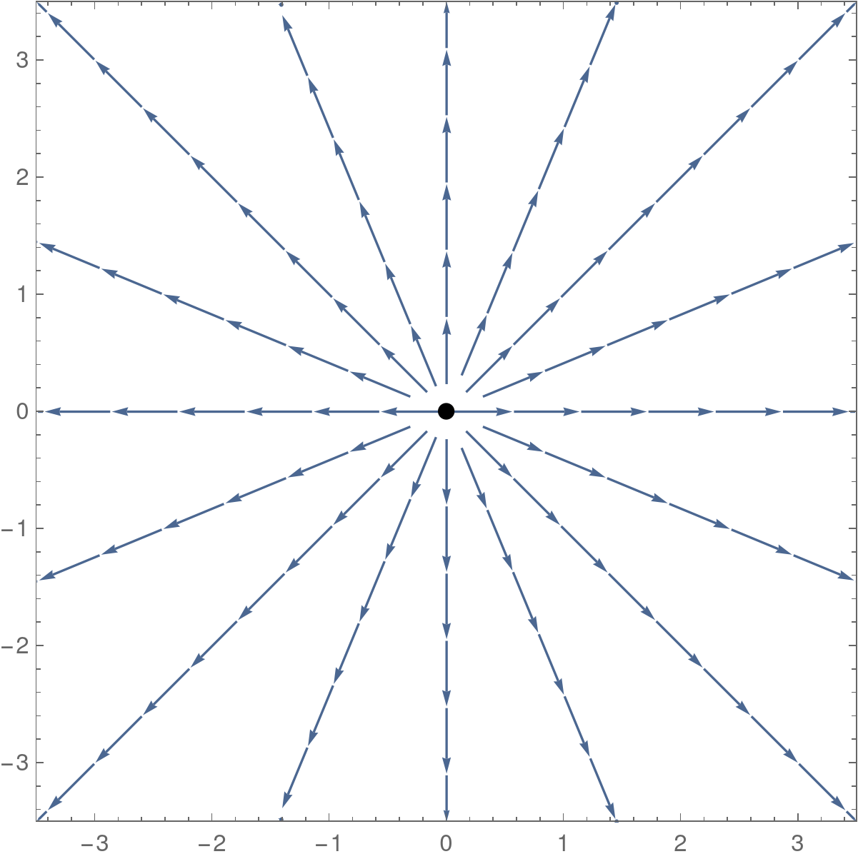
(c) aster

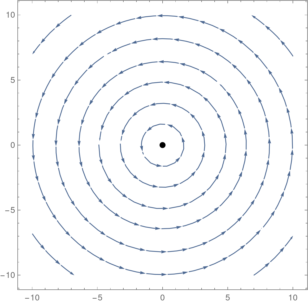
(d) vortex

Figure 1: Sketches of single defect textures showing the angle $\phi_{i}$ (the phase of $P_{i}$) for (a) a $+1$ defect where $\phi_{i}$ is the angle between $P_{i}$ and $\hat{r}$, (b) a $-1$ defect where $\phi_{i}/2$ is the angle of the separatrix. Special values of $\phi_{i}$ are shown in (c) and (d) for a $+1$ defect: (c) is an aster ($\phi_{i}=0$), and (d) is a vortex ($\phi_{i}=\pi/2$).

Finally, we note that for a global rotation, under which $z\to e^{i\eta}z$, the complex order parameter transforms as $p_{0}\to p_{0}e^{i\eta(1-\sum_{i}\sigma_{i})}$. This implies that if $\sum_{i}\sigma_{i}\neq 1$, we can choose $\eta$ such that it eliminates the global phase factor $\psi$. In particular, we cannot eliminate the phase for a single $+1$ defect. This obstruction is not surprising since $+1$ defects are unique among defects in that they are rotationally invariant as $p\propto z$. We will see in our analysis that $\psi$ plays a crucial role for $+1$ defects.

IV Dynamics of active polar defects (interactions)

IV.1 Method

We are interested in solving the following PDE:

$$\frac{\partial p}{\partial t}=\mathcal{I}(p)$$ (15)

We do so by following the variational method used in Zhang et al. (2020); Vafa et al. (2020), which we now review. We start by making the ansatz

$$p(z,\bar{z},t)=p_{0}(z,\bar{z},\{w_{a}(t)\})$$ (16)

where $w_{a}(t)$ (perhaps infinitely many) are parameters that need to be specified. (For example, $w_{a}(t)$ can include the defect positions, but is not strictly limited to them.) Once specified, $w_{a}(t)$ are computed by minimizing the deviation of $dp_{0}/dt$ from that described by the equation of motion, Eq. (7). In other words, we minimize the error

$$E =\int d^{2}dzd\bar{z}\left|\partial_{t}p(z,{\bar{z}},t)-\frac{d}{dt}p_{0}(z,{\bar{z}}|\{w_{a}(t)\})\right|^{2}$$

$$\approx\int dzd\bar{z}\left|\mathcal{I}(p_{0})-\dot{w}_{a}\frac{\partial p_{0}}{\partial w_{a}}\right|^{2}$$ (17)

with respect to $\dot{w}_{a}$, where $\mathcal{I}$ is defined in Eq. (7). Of course, the goodness of our minimization depends on the ansatz and the chosen parameters $w_{a}$. We choose our ansatz to be $p_{0}$, because we know that when the defects are fixed and when $\lambda=0$, $p_{0}$ is a good solution Pacard and Rivière (2000). Specifically, we assume that the defects are far away from each other and that $\lambda\ll 1$, in which case $p_{0}$ is a quasi-static solution to Eq. (7). Taking into account that $\lambda\neq 0$ and the defects are not infinitely far away from each other leads to motion of the defects, and we will assume that the time-dependence of $p$ is only through the defect positions $z_{i}(t)$, and that the motion is slow. In other words, we will make the ansatz

$$p(z,\bar{z},t)=p_{0}(z,\bar{z},\{z_{i}(t)\})$$ (18)

where we have chosen $w_{a}(t)$ to be $z_{i}(t)$, the defect positions.

Doing so, one finds that Vafa et al. (2020)

$$\mathcal{M}_{ij}\dot{z}_{j}+\mathcal{N}_{ij}\dot{\bar{z}}_{j}=-\frac{\partial{\mathcal{F}}_{0}}{\partial\bar{z}_{i}}+\lambda{\mathcal{U}}_{i}\;,$$ (19)

where

$$\mathcal{M}_{ij} =\int d^{2}z[\bar{\partial}_{i}\bar{p}_{0}\partial_{j}p_{0}+\bar{\partial}_{i}p_{0}\partial_{j}\bar{p}_{0}]$$ (20)

$$\mathcal{N}_{ij} =\int d^{2}z[\bar{\partial}_{i}\bar{p}_{0}\bar{\partial}_{j}p_{0}+\bar{\partial}_{i}p_{0}\bar{\partial}_{j}\bar{p}_{0}]\;.$$ (21)

are the mobility matrices,

$$\mathcal{F}_{0}=-2\pi\sum_{i\not=j}\sigma_{i}\sigma_{j}\ln\frac{|z_{i}-z_{j}|}{L}\;,$$ (22)

is the Coulomb free energy, and

$${\mathcal{U}}_{i}=\int d^{2}z[\bar{\partial}_{i}\bar{p}_{0}\mathcal{I}_{\lambda}+\bar{\partial}_{i}p_{0}\bar{\mathcal{I}}_{\lambda}]\;.$$ (23)

The mobility matrices $\mathcal{M}_{ij}$ and $\mathcal{N}_{ij}$ have been calculated in Vafa et al. (2020) to be

$$\mathcal{M}_{ij} \approx\pi\sigma_{i}\sigma_{j}\ln\frac{L}{r_{ij}}$$ (24)

$$\mathcal{N}_{ij} \approx 0\;.$$ (25)

Before proceeding, we would like to emphasize that in order to determine $z_{i}$, we are doing a global fit within our ansatz that finds the $z_{i}$ that minimizes the error. That is to say, although we interpret $z_{i}$ as the positions of defects, $z_{i}$ are simply parameters in our ansatz for the global texture that act as a proxy for the defect positions, and similarly $\dot{z}_{i}$ are not the true velocities of the defects. If we were interested in calculating the exact defect velocities, then we could do so with a local calculation which tracks the zeros of $p$. However, we are interested in how $p$ evolves everywhere, not just at specific points, which is why we minimize the error $E$ in Eq. (17). Note that the fact that our equations depend on the system size $L$ is not surprising given we are doing a global fit in a region of size $L$. And, we have the freedom, if we are interested, to focus on the physics in a subregion of size $\ell<L$ by minimizing Eq. (17) in this subregion.

IV.2 Interactions

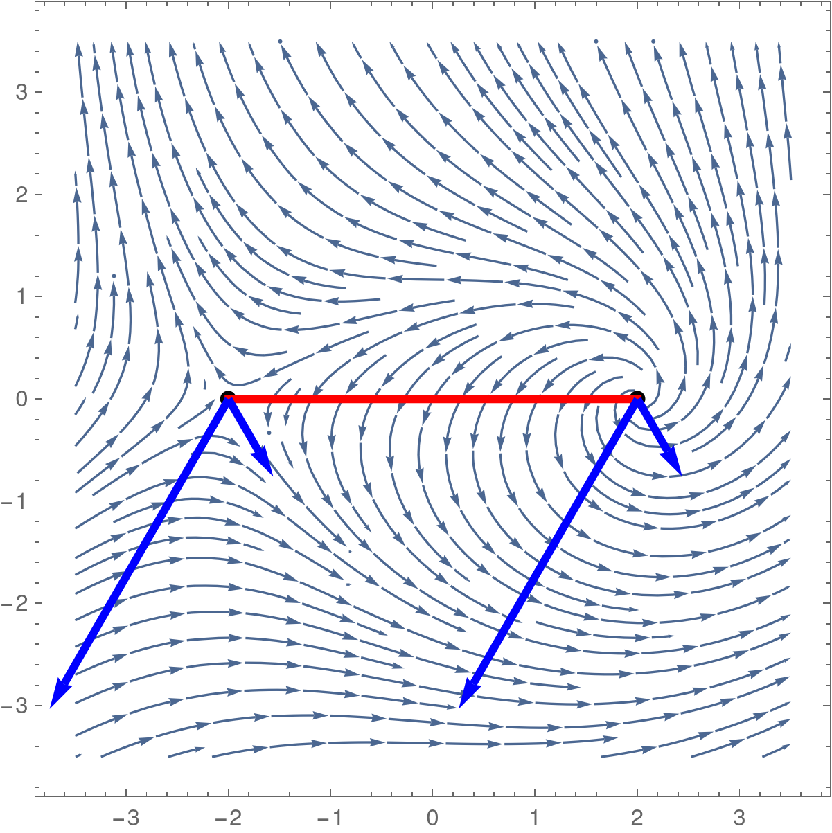
(a) $-1$ and $+1$ defects

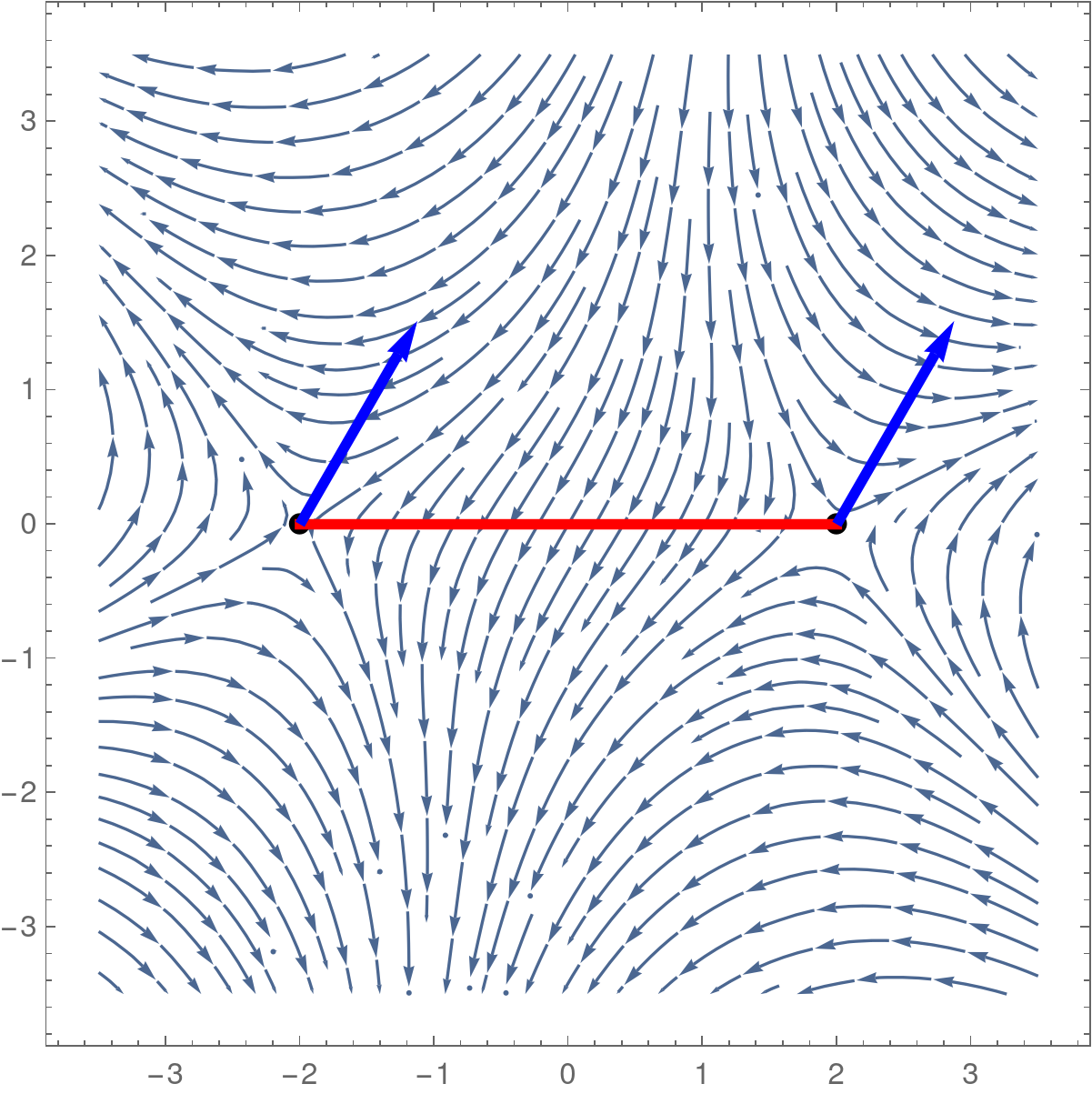
(b) $-1$ and $-1$ defects

Figure 2: Sketches of the active forces $f_{ij}$ for $\lambda>0$. The blue arrows denote the two components of the active force $f_{ij}$, and the red line joins the center of the two defects. For each pair, $f_{ij}=f_{ji}$, and the net forces are generically non-central.

In Appendix B, we show that $\mathcal{U}_{i}$ (defined in Eq. (23)) can be explicitly written in terms of the defect positions as

$$\lambda\mathcal{U}_{i}=-8\pi\ln\frac{L}{a}\lambda\bar{P}_{i}\delta_{\sigma_{i},2}+\sum_{j\neq i}f_{ij},$$ (26)

where in terms of the unit vector $\hat{z}_{ij}=(z_{i}-z_{j})/|z_{i}-z_{j}|$ and its complex conjugate $\hat{\bar{z}}_{ij}$,

$$f_{ij}=\frac{1}{2}\lambda\sigma_{i}\sigma_{j}\hat{z}_{ij}\left(P_{i}\hat{z}_{ij}^{\sigma_{i}-1}I^{(1)}_{ij}-\bar{P}_{i}\hat{\bar{z}}_{ij}^{\sigma_{i}-1}I^{(2)}_{ij}\right)\;$$ (27)

with

$$I^{(1)}_{++}=I^{(1)}_{--}=2\pi$$

$$I^{(1)}_{+-}=I^{(1)}_{-+}=2\pi\ln\frac{L}{r_{ij}}+\mathcal{O}(L^{0})$$

$$I^{(2)}_{++}=2\pi\ln\frac{L}{r_{ij}}+\mathcal{O}(L^{0});\quad I^{(2)}_{--}=0$$

$$I^{(2)}_{+-}=I^{(2)}_{-+}=2\pi\;.$$ (28)

The first term in Eq. (26) is the “self-propulsion” of a $+2$ defect along the $\bar{P}_{i}$ direction, where $P_{i}$ was defined in Eq. (14). Of course, we should not take this term too seriously, because a $+2$ defect can be interpreted as a bound state of two $+1$ defects, which is unstable because of the Coulomb repulsion. The second term in Eq (26) is the active induced pair-wise interaction, and its leading dependence on distance $r_{ij}$ between two defects $i$ and $j$ is $\ln L/r_{ij}$.

We now examine the net force. Since $I^{(1)}_{ij}\neq I^{(2)}_{ij}$, then $f_{ij}$ is a generic non-central force; in particular, it is also not orthogonal to the line connecting the two defects. We also comment that since $f_{ij}=f_{ji}$, then the defect pair moves together, as if it is a bound object. Another feature is that for a pair of $-1$ defects, there is no dependence on the distance between the defects, unlike in cases of the neutral pair or pair of $+1$ defects. See Fig. 2 and Fig. 3 for sketches.

We have learned that two $+1$ defects exert the same force on each other (same magnitude and direction), as if they’re bound. In the limit that these defects are really close to each other, then there is no reason a priori to expect that they are actually bound, as our assumptions no longer hold. However, interestingly enough, the two defects behave as if they’re a $+2$ defect, a bound state of two $+1$ defects, which is “self-propelled” in the same direction, along its separatrix, consistent with the behavior of a $+2$ defect (see Fig. 3). This did not have to be the case, and does not hold for the other defect pairs.

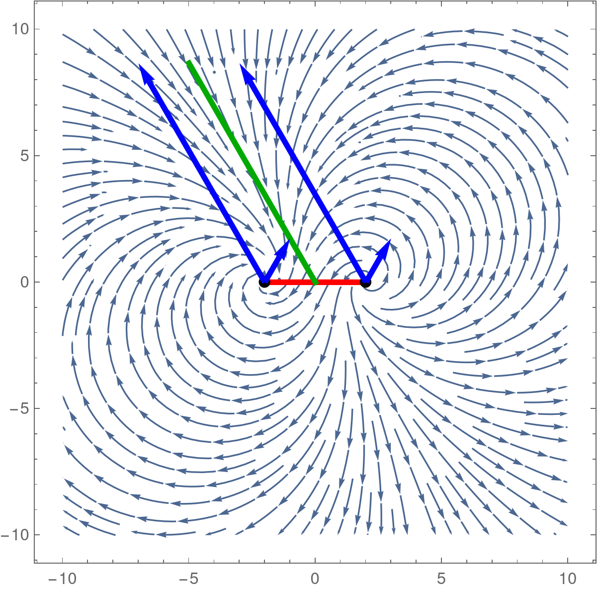
(a) Two $+1$ defects

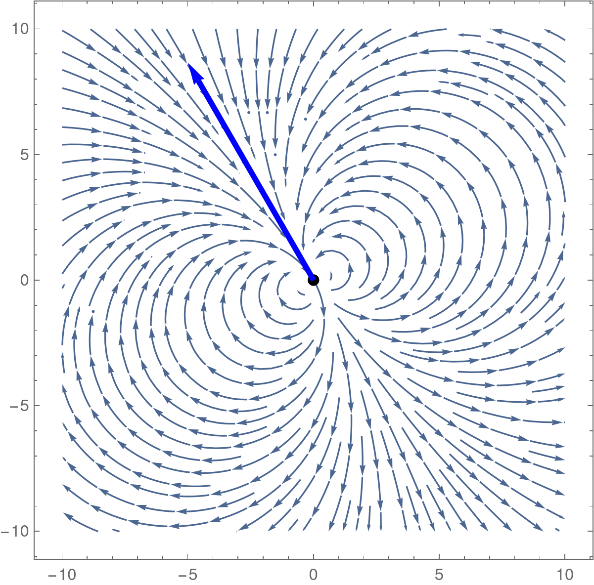
(b) A single $+2$ defect

Figure 3: Sketches of active forces with $\lambda>0$ for (a) two $+1$ defects, and (b), for a single $+2$ defect (the “self-propulsion” force). The forces for both cases are essentially in the same direction.

V Orientation dynamics

In the previous section, we ignored orientation dynamics. We now incorporate orientation dynamics and sketch out the argument here (the details of the computation are in Appendix C). For simplicity, we consider a single defect of charge $\sigma$ at the origin, in which case our ansatz is

$$p_{0}=e^{i\psi(t)}\left(\frac{z}{|z|}\right)^{\sigma}\;,$$ (29)

where now the phase $\psi(t)$ is dynamical. Choosing $w_{a}(t)=\psi(t)$ in Eq. 17 leads to

$$\int d^{2}z|\frac{\partial p}{\partial\psi}|^{2}\dot{\psi}=\frac{\lambda}{2}\int d^{2}z\frac{\partial\bar{p}}{\partial\psi}\mathcal{I}_{\lambda}+c.c$$ (30)

and upon evaluation in a region of size $\ell$ near the defect, where $a\ll\ell\ll L$ and $a$ is the core size,

$$\pi\ell^{2}\dot{\psi}=-2\pi\lambda\ell\sin\psi\delta_{\sigma,1}\implies\dot{\psi}=-2\frac{\lambda}{\ell}\sin\psi\delta_{\sigma,1}\;.$$ (31)

Only the solution for $+1$ defects is nontrivial, which for completeness is given by

$$\psi(t)=2\,\rm{arccot}\left(e^{\frac{2\lambda}{\ell}t}\cot\left(\frac{\psi(0)}{2}\right)\right)\;.$$ (32)

Note that we can interpret Eq. 31 as relaxational dynamics

$$\dot{\psi}=-\frac{2}{\ell}\frac{dV}{d\psi}$$ (33)

for the potential $V=-\lambda\cos\psi$ (see Fig. 4 for a plot). Thus for $\lambda>0$, the defect will relax to an aster ($\psi=0$), and for $\lambda<0$, the defect will relax to an inward-pointing aster ($\psi=\pi$).. In other words, there is a preferred phase. Stable asters have been observed in related simulations Aranson and Tsimring (2005, 2006); Elgeti et al. (2011); Gopinath et al. (2012); Gowrishankar and Rao (2016); Husain and Rao (2017), as well as analyzed in related models Youn Lee and Kardar (2001); Sankararaman et al. (2004); Kruse et al. (2004, 2005); Elgeti et al. (2011).

We also check our theory with simulations. We evolve an isolated $+1$ defect for nonzero $\lambda=1$, where initially the phase $\psi(0)=\pi/2$. We computed the phase in two different ways: a local computation, which locates the $+1$ defect and measures the phase, and a global computation, which calculates the defect position and phase by minimizing in a region of size $\ell=30a\ll L=300a$ the deviation of our ansatz $p_{0}$ from the measured $p_{0}$, which is basically equivalent minimizing Eq. (17), as we did in deriving Eq. (31). We find that initially and at long times, the two different measurements of the phase agree, and even though they are not identical in the middle, they both are similar. Moreover, we checked our measured global definition of $\psi(t)$ vs that predicted from theory obtained by integrating Eq. (33), and find remarkable agreement (see Fig. 5).

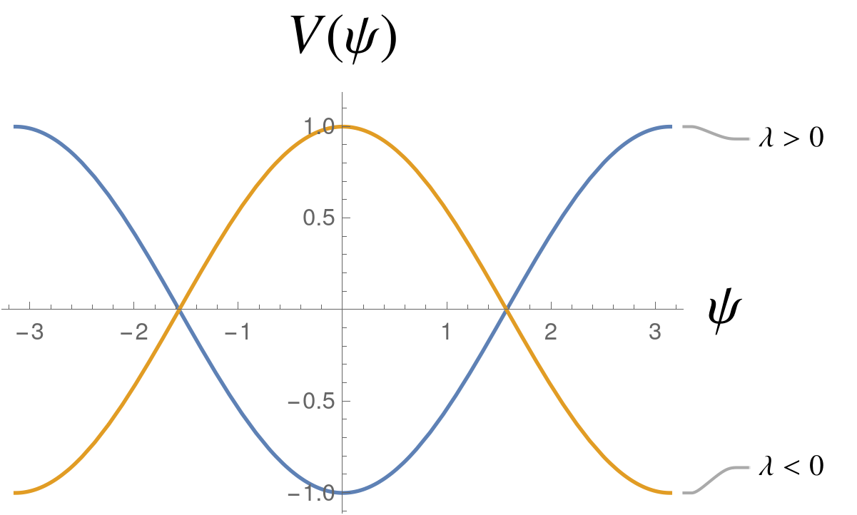
Figure 4: Plot of $V(\psi)$ for $\lambda>0$ and $\lambda<0$. Extrema are at $\psi=0,\pi$. Minimum for $\lambda>0$ is at $\psi=0$, whereas minimum for $\lambda<0$ is at $\psi=\pi$.

Given that our method suggests that there appear to be two different stationary solutions for $+1$ defects (aster or inward-pointing aster, depending on the sign of $\lambda$), it raises the question whether these solutions are stationary solutions of Eq. (7). By inspection, $+1$ defects, in particular asters or inward-pointing asters, are indeed stationary solutions of Eq. (7).

Since the phase appears to be important, it is natural to ask if we can modify our ansatz in Eq. (18) to take into account the phase, for example by taking $\Psi_{i}\to e^{i\phi_{i}f(|z-z_{i}|)}\Psi_{i}$, where for example as in Tang and Selinger (2017) $f(|z-z_{i}|)=e^{i\gamma_{i}\ln|z-z_{i}|}$ . We leave this analysis to future work.

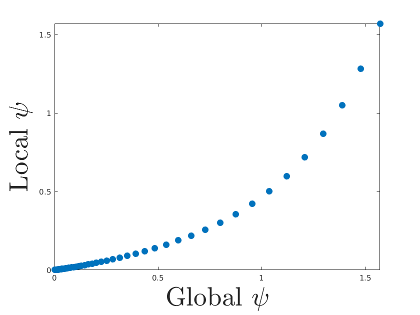
(a) $+1$ defect

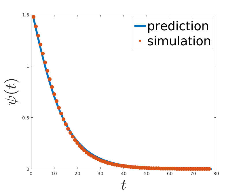
(b) $-1$ defect

Figure 5: Dynamics of the phase $\psi(t)$ of a single $+1$ defect for $\lambda>0$ with $\psi(0)=\pi/2$. In (a), plot of local computation vs global computation of the phase $\psi$ for a single $+1$. Their ending points are the same, but they are not identical in the middle. In (b), theoretical prediction vs simulation of $\psi(t)$.

VI Stationary solution through scaling argument

In this paper, we have focused on defects. Here we make contact with the discussion contained in Chaté (2020), and provide another perspective about why defects are transient in active polar fluids.

We make use of a scaling argument. By inspection, there is a scaling symmetry; that is, solutions obey

$$p(z,t;\lambda)=p(z/\beta,t/\beta^{2};\beta\lambda)\;.$$ (34)

We are interested in the stationary, longtime behavior, which means that we are looking for $p$ such that for any $t$

$$\lim_{\gamma\to\infty}\frac{\partial}{\partial t}p(z,\gamma^{2}t;\lambda)=0\;.$$ (35)

From our scaling relation in Eq. 34, choosing $\beta=\gamma$ is equivalent to finding $p$ such that

$$\lim_{\gamma\to\infty}\frac{\partial}{\partial t}p(z/\gamma,t;\gamma\lambda)=0\;.$$ (36)

We thus look for steady states for large $\lambda$. For large $\lambda$, the advection term in Eq. (7) dominates, and thus long-time stationary states satisfy

$$\partial_{t}p=-\lambda(p\partial+\bar{p}\bar{\partial})p=0\;.$$ (37)

We will now show that the only solutions to the above equation other than constant $p$ is a single aster or inward-pointing aster, which as we commented in Sec. V satisfies the above equation. Because we are deep in the ordered phase, our ansatz is $p=\frac{f(z)}{\bar{f}(\bar{z})}$. Then

$$\partial_{t}p=-\lambda(p\partial+\bar{p}\bar{\partial})p=-\frac{\lambda}{\bar{f}^{2}}(f\partial f-\bar{f}\bar{\partial}\bar{f})$$ (38)

which vanishes only if $\partial(f^{2})=c_{1}$, where $c_{1}\in\mathbb{R}$. Therefore, $f^{2}=c_{1}z+c_{2}$, and so $p$ is constant if $c_{1}=0$, and otherwise

$$p=e^{i\psi}\frac{(z-z_{i})^{1/2}}{(\bar{z}-\bar{z}_{i})^{1/2}}$$ (39)

where either $\psi=0$ (aster) or $\psi=\pi$ (inward pointing aster), depending on the sign of $\lambda$; no other $\psi$ is allowed. Note that this single aster stationary state is consistent with the single vortex to aster transition, as in Eq. (33). We have thus provided another perspective for transient behavior of defects.

VII Comparison with active nematics model

VII.1 Overview

In this section, we compare our model to the active nematics model studied in Vafa et al. (2020). We first present a general overview, and then study the consequences. The similarities are that both models advect an order parameter deep in the ordered phase and in the overdamped limit. In the case of nematic, the order parameter is a rank 2 symmetric traceless tensor $\mathbf{Q}$, and in the case of polar, the order parameter is a vector. This difference implies that there are extra terms in the advection of $\mathbf{Q}$. In the case of nematic, overdamped limit implies $\mathbf{v}=\alpha\nabla\cdot\mathbf{Q}$, where $\alpha$ is a measure of activity, and in the case of polar, $\mathbf{v}=\lambda\mathbf{p}$. This difference in dependence of length scaling implies that in the nematic model, $\alpha$ cannot be scaled out of the problem, but in the polar model, $\lambda$ can be scaled out. Although these models are different, they are similar, and by studying these models in depth it is interesting to learn which features are common and which are model-dependent.

VII.2 Forces

We now compare the forces. In the absence of activity, the models are equivalent. The forces that arise because of activity are different. In the active nematics case, a $+1/2$ defect, the smallest allowed energy excitation, is “self-propelled”, whereas in the active polar case, a $\pm 1$ defect, the smallest allowed energy excitation, is not “self-propelled”; a $+2$ defect is “self-propelled”. Another difference between these two models arise in the pair-wise interactions induced by activity. In the active nematics case, the active forces are central for a $(+1/2,+1/2)$ pair, and for the other pairs are orthogonal to line connecting the defects. Also, the forces for $(+1/2,-1/2)$ pair are non-reciprocal. All of these forces fall off as $1/r$, where $r$ is the distance between the defects, and the magnitude depends on the geometry, that is, overall phase of $Q$. In contrast, in the case of active polar, the active forces are neither central forces nor orthogonal to the line connecting the two defects. They are also always equal, and except for the $-1$ defect pair, goes as $\ln L/r$. Similar to active nematic, the magnitude of the force depends on the geometry, that is, the phase of $p$.

VII.3 Orientation dynamics / solutions

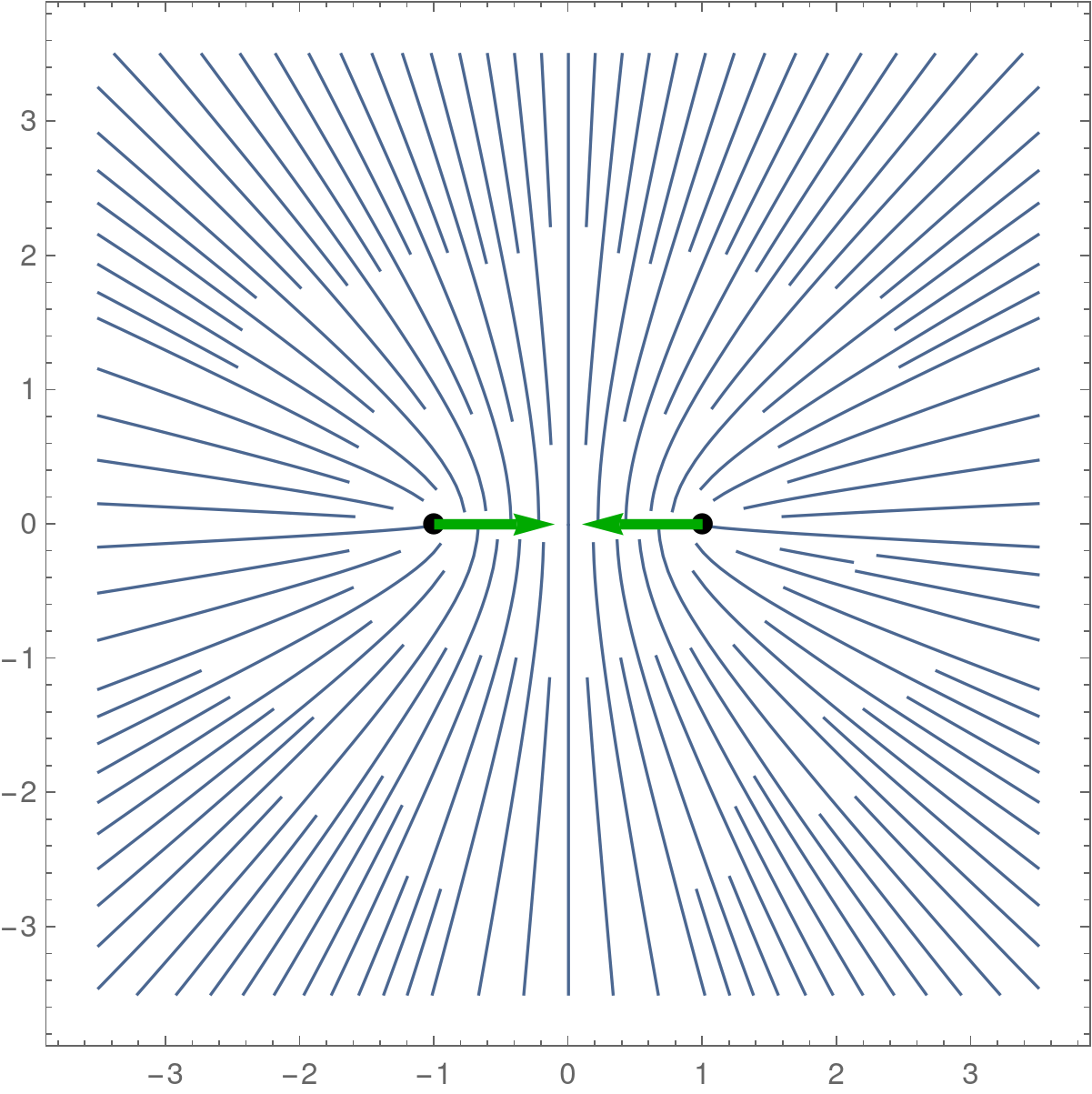
(a) Aster bound state

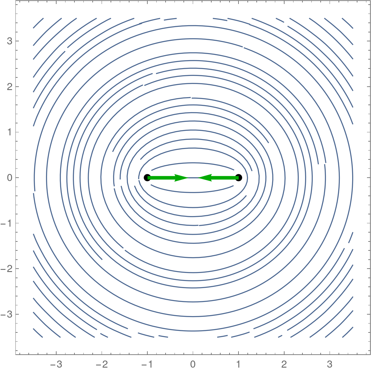
(b) Vortex bound state

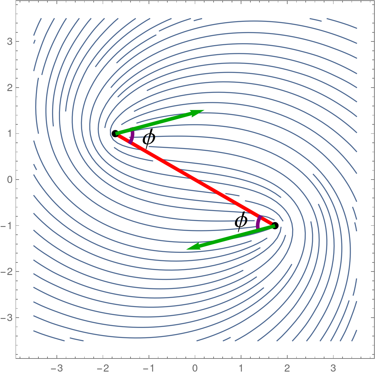
(c) Spiral bound state

Figure 6: In active nematics model, sketches of bound state of two $+1/2$ defects. In (a), bound aster state in extensile system when $\psi=0$, (b), bound vortex state in contractile system when $\psi=\pi$, and in (c), bound spiral state in contractile system when $0<\psi<\pi/2$.

In this paper, we learned that $+1$ asters (inward-pointing asters) are stationary solutions and that they are stable for $\lambda>0$ ($\lambda<0$). It is natural to ask whether in the nematic model there can be stationary $+1$ defect configurations, and does the existence of solutions, or stability, depend on the phase of the defects. We show that indeed solutions exist, and the type of solution depends on the phase of the defects.

We first check to see what happens if we incorporate orientation dynamics into the active nematics model. The active nematics model has the following equation of motion,

$$\partial_{t}Q=\mathcal{I}(Q)=-\frac{\delta{\mathcal{F}}(\{Q\})}{\delta{\bar{Q}}}+\alpha\mathcal{I}_{\alpha}(Q)\;,$$ (40)

where

$$\frac{\delta{\mathcal{F}}(\{Q\})}{\delta{\bar{Q}}}=-4{\bar{\partial}}\partial Q-2\epsilon^{-2}(1-|Q|^{2})Q$$ (41)

$$\mathcal{I}_{\alpha}(Q)=-(\partial Q\partial Q+{\bar{\partial}}{\bar{Q}}{\bar{\partial}}Q)+(\partial^{2}Q-\bar{\partial}^{2}\bar{Q})Q$$ (42)

We work in the deep nematic limit ($\epsilon\to 0$). For simplicity, we consider a single defect of charge $\sigma=\pm 1/2$ at the origin, in which case our ansatz is

$$Q_{0}=e^{i\psi(t)}\left(\frac{z}{\bar{z}}\right)^{\sigma}\;,$$ (43)

where now the phase $\psi(t)$ is dynamical. Minimizing the error

$$E =\int d^{2}dzd\bar{z}\left|\partial_{t}Q(z,{\bar{z}},t)-\frac{d}{dt}Q_{0}(z,{\bar{z}}|\psi(t))\right|^{2}$$

$$\approx\int dzd\bar{z}\left|\mathcal{I}(Q_{0})-\dot{\psi}\frac{\partial Q_{0}}{\partial\psi}\right|^{2}$$ (44)

with respect to $\dot{\psi}$ (the analogue of Eq. (17)) leads to

$$\int d^{2}z|\frac{\partial Q_{0}}{\partial\psi}|^{2}\dot{\psi}=\frac{\alpha}{2}\int d^{2}z\frac{\partial\bar{Q}_{0}}{\partial\psi}\mathcal{I}_{\alpha}+c.c$$ (45)

(the analogue of Eq. (19)). We now evaluate both sides of this equation in a region near the defect of size $\ell$. As before,

$$\int d^{2}z|\frac{\partial Q_{0}}{\partial\psi}|^{2}=\pi\ell^{2}$$ (46)

We now evaluate the RHS. We have

$$\int d^{2}z\frac{\partial\bar{Q}_{0}}{\partial\psi}\mathcal{I}_{\alpha}+c.c=$$ (47)

$$-i\int d^{2}z[-\sigma^{2}(\frac{Q_{0}}{z^{2}}-\frac{\bar{Q}_{0}}{\bar{z}^{2}})+\sigma(\sigma-1)(\frac{Q_{0}}{z^{2}}-\frac{\bar{Q}_{0}}{\bar{z}^{2}})]+c.c$$

$$=0$$ (48)

which implies that

$$\dot{\psi}=0$$ (49)

and we thus learn that the phase is frozen, in accordance with the expectation in Vafa et al. (2020). Here there is no preferred orientation, unlike in the active polar case, where asters or anti-asters are preferred, depending on the sign of $\lambda$.

In related models, $+1$ defect states consisting of two $+1/2$ defects have been observed in active nematics Kumar et al. (2018); Pearce et al. (2020); Thijssen et al. (2020), and in Shankar et al. (2018); Thijssen and Doostmohammadi (2020), it was argued that the type of $+1$ defect was determined by the activity: asters in extensile systems, and vortices in contractile systems. This observation is related to our result of finding a stationary $+1$ defect in the active polar model, as we will now see. We now review and present another argument for the existence and stability of a stationary defect pair of two $+1$ defects in the active nematics case.

Let’s consider two $+1/2$ defects situated on the real axis. The orientations of the $+1/2$ defects anti-align Vromans and Giomi (2016); Pearce et al. (2020); Thijssen et al. (2020); Vafa et al. (2020). For simplicity, let’s assume that the orientations are along the real axis, so they either point away from each other (phase is 0), or toward each other (phase is $\pi$). There are four forces: the defect drag force, the repulsive Coulomb force, the self-propulsion, and the active induced pair-wise force. We will ignore the defect drag force and active induced pair-wise force because they renormalize the velocity and Coulomb force, respectively. In this case, for $\alpha>0$ (contractile), the $+1/2$ defects move with constant velocity in the direction of their phase, and for $\alpha<0$ (extensile), the $+1/2$ defects move with constant velocity in the opposite direction of their phase. Therefore, at a unique separation $r_{*}$ the repulsive Coulomb force can balance the attractive self-propulsion force depending on the sign of $\alpha$ and the phase. The configuration is stationary for either extensile system and phase is $0$ or contractile system and phase is $\pi$. In the former, the two $+1/2$ defects form a bound aster state, and in the latter, they form a bound vortex state (see Fig. 6). This argument was pointed out in Shankar et al. (2018); Turiv et al. (2020); Thijssen and Doostmohammadi (2020).

Moreover, this bound state is stable to transverse fluctuations of the polarization Shankar et al. (2018). Here we present an alternative argument. If the defects are not exactly aligned, one would naively think that the self-propulsion will cause the $+1/2$ defects to go away from each other. However, we will now show that as the defects move, the orientation readjusts in such a way that it leads to inward spiral motion of the pair of defects. From arguments presented in Vafa et al. (2020), in terms of this phase $\phi$ (the angle of the orientation, that is, the deviation from radial line connecting the two defects), the solution takes the form

$$Q(z,t)=e^{i\phi}\frac{z-z_{i}(t)}{|z-z_{i}(t)|}\frac{z-z_{j}(t)}{|z-z_{j}(t)|}$$ (50)

where $z_{i}$ and $z_{j}$ are the positions of defects $i$ and $j$, respectively. The orientation $Q_{i}(t)$ of defect $i$ is simply

$$Q_{i}(t)=e^{i\phi}\frac{z_{i}(t)-z_{j}(t)}{|z_{i}(t)-z_{j}(t)|}$$ (51)

Since $+1/2$ defects are self-propelled along their orientation, in the direction of $Q_{i}$, then they will always move at a constant angle $\phi$ relative to the radial line connecting the two defects. Thus for example in contractile system, if $\phi$ is sufficiently close to $0$, and the activity is not too large, then the two defects will simply spiral towards each other (see Fig. 6). The solution is thus stable, but not stationary.

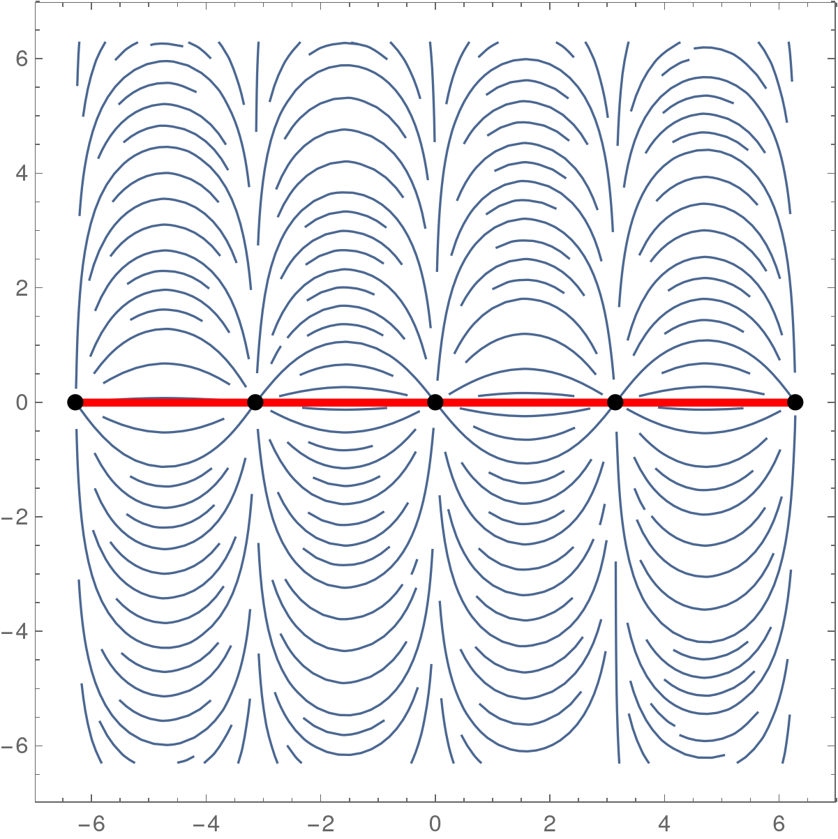
(a) Asters

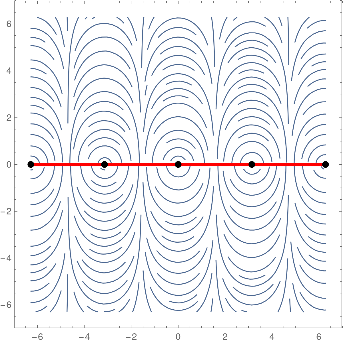
(b) Vortices

Figure 7: Configuration of 1D chain of equally spaced $+1$ defects for active nematics model that screens the activity term.

Given that it seems that a composite made of a pair of $+1/2$ defects is a stationary solution for the active nematic model and far away it looks like an aster or vortex, it is natural to ask if an aster or vortex is actually a solution to Eq. (40). By inspection, indeed a nontrivial solution is $Q=\pm\frac{z}{\bar{z}}$ (as one can easily check that the active term $\mathcal{I}_{\alpha}=0$), where the $+$ sign corresponds to an aster and the $-$ sign corresponds to a vortex. Note that this solution of aster or vortex is consistent with the picture in Fig. 6, as any other phase results in a non-stationary state. Thus a single aster or a vortex is indeed a stationary solution to Eq. (40).

Screening of activity term by $+1$ defects in active nematics is similar to what we found in active polar fluids. In active polar fluids, this is the only configuration which screens the active term and that is the reason for transient behavior of defects. Is this the case in active nematics or are there more general configurations that screen the active term? Or can we extend this solution to allow multiple defects? A natural place to look for this (ignoring the passive forces) is to look for configurations that screen the active term ($\mathcal{I}_{\alpha}=0$), as in the case of single aster/vortex. In the polar case, a single aster was the only defect configuration that screened the active term. Here we will see that the situation (and solution) is more interesting for a nematic system.

We are thus interested in solving

$$\mathcal{I}_{\alpha}=0\;,$$ (52)

where

$$\mathcal{I}_{\alpha}=-\partial Q\partial Q-{\bar{\partial}}{\bar{Q}}{\bar{\partial}}Q+(\partial^{2}Q-\bar{\partial}^{2}\bar{Q})Q$$ (53)

Deep in the ordered phase, $Q=\pm e^{i(f(z)+\bar{f}(\bar{z}))}$, and so

$$iQ\left(\partial^{2}fe^{2if}+\bar{\partial}^{2}\bar{f}e^{-2i\bar{f}}\right)=0$$ (54)

Other than the constant solution, the unique solution is

$$f(z)=-i\ln\sin k(z-z_{0})$$ (55)

where without loss of generality we can assume $k\in\mathbb{R}$ by rotation of $z$ coordinate if necessary and place the origin at $z_{0}$. Therefore,

$$Q=\pm e^{i(f(z)+\bar{f}(\bar{z}))}=\pm\frac{\sin kz}{\sin k\bar{z}}\;.$$ (56)

Notice that this vanishes at $z=n\pi/k$, for $n\in\mathbb{Z}$, and near each zero, $Q\sim\pm\frac{z}{\bar{z}}$. We thus have an infinite chain of $+1$ nematic defects on the real axis, separated by $\pi/k$. Because of the sign of $Q$, either the defects are all asters (when the sign is positive), or the defects are all vortices (when the sign is negative). These configurations are depicted in Fig. 7.

Ignoring the Coulomb term, we have analytically found a stationary $1D$ lattice solution. For example, in the geometry of a thin annulus (or equivalently, long channel with periodic boundary conditions), we can imagine that the boundary condition balances the Coulomb forces. In any case, this shows that $\mathcal{I}_{\alpha}=0$ has a much more interesting set of solutions than $\mathcal{I}_{\lambda}=0$, and deserves further study, pointing to the importance of defects in active nematic systems as opposed to active polar systems.

Appendices

Appendix A Single defect solution

Stationary textures in the limit of zero activity ($\lambda=0$) minimize free energy and hence solve  De Gennes and Prost (1993); Pismen (1999)

$$\frac{\delta{\mathcal{F}}}{\delta{\bar{p}}}=-\nabla^{2}p-2\epsilon^{-2}(1-|Q|^{2})p=0\;.$$ (57)

We look for a solution for a single defect of charge $\sigma$ of the form

$$p=A(r)e^{i\sigma\varphi}\;.$$ (58)

$A(r)$ would thus satisfy

$$A^{\prime\prime}(r)+\frac{A^{\prime}}{r}+\left(2\epsilon^{-2}-\frac{\sigma^{2}}{r^{2}}-2\epsilon^{-2}A^{2}\right)A=0\;.$$ (59)

For example, for $\sigma=\pm 1$, $A(r)$ can be approximated as Pismen (1999)

$$A(r)=\tilde{r}\sqrt{\frac{.68+.28\tilde{r}^{2}}{1+.82\tilde{r}^{2}+.28\tilde{r}^{4}}}\;,$$ (60)

where $\tilde{r}=r/\epsilon$. As $r\to 0$, $A(r)\propto r$, and for $r\gg\epsilon$, $A(r)\simeq 1-\frac{\epsilon^{2}}{4r^{2}}$. The defect core size $a$, which is the length scale over which $A$ goes from 0 to 1, is of the order $a\sim\epsilon$.

Appendix B Computation of $\mathcal{U}_{i}$

We are interested in computing

$$\mathcal{U}_{i}=\int d^{2}z\bar{\partial}_{i}\bar{p}_{0}\mathcal{I}_{\lambda}+\int d^{2}z\bar{\partial}_{i}p_{0}\bar{\mathcal{I}}_{\lambda}=I_{1}+I_{2}\;,$$ (61)

where

$$I_{1} =-\int d^{2}z\bar{\partial}_{i}\bar{p}_{0}p_{0}\partial p_{0}-\int d^{2}z\bar{\partial}_{i}p_{0}p_{0}\partial\bar{p}_{0}$$ (62)

$$I_{2} =-\int d^{2}z\bar{\partial}_{i}p_{0}\bar{p}_{0}\bar{\partial}\bar{p}_{0}-\int d^{2}z\bar{\partial}_{i}\bar{p}_{0}\bar{p}_{0}\bar{\partial}p_{0}\;.$$ (63)

Substituting for $p_{0}$, we find that

$$I_{1} =\frac{1}{2}\sum_{j}\int d^{2}zp_{0}\frac{\sigma_{i}\sigma_{j}}{(\bar{z}-\bar{z}_{i})(z-z_{j})}$$ (64)

$$I_{2} =-\frac{1}{2}\sum_{j}\int d^{2}z\bar{p}_{0}\frac{\sigma_{i}\sigma_{j}}{(\bar{z}-\bar{z}_{i})(\bar{z}-\bar{z}_{j})}$$ (65)

It is convenient to rewrite the above as

$$I_{1} =\frac{1}{2}\int d^{2}zp_{0}\frac{\sigma_{i}^{2}}{|z-z_{i}|^{2}}+\frac{1}{2}\sum_{j\neq i}\int d^{2}zp_{0}\frac{\sigma_{i}\sigma_{j}}{(\bar{z}-\bar{z}_{i})(z-z_{j})}$$ (66)

$$I_{2} =-\frac{1}{2}\int d^{2}z\bar{p}_{0}\frac{\sigma_{i}^{2}}{(\bar{z}-\bar{z}_{i})^{2}}-\frac{1}{2}\sum_{j\neq i}\int d^{2}z\bar{p}_{0}\frac{\sigma_{i}\sigma_{j}}{(\bar{z}-\bar{z}_{i})(\bar{z}-\bar{z}_{j})}$$ (67)

The first term for $I_{1}$ vanishes by phase integral. The first term for $I_{2}$ is only non-zero for $\sigma_{i}=2$, in which case (since we are assuming that defects are well-separated), we can approximate

$$-\frac{1}{2}\int d^{2}z\bar{p}_{0}\frac{\sigma_{i}^{2}}{(\bar{z}-\bar{z}_{i})^{2}} \approx-\delta_{\sigma_{i},2}\frac{1}{2}\bar{P}_{i}\int d^{2}z\frac{(\bar{z}-\bar{z}_{i})^{2}}{|z-z_{i}|^{2}}\frac{4}{(\bar{z}-\bar{z}_{i})^{2}}$$

$$=-8\pi\bar{P}_{i}\delta_{\sigma_{i},2}\ln\frac{L}{a}$$ (68)

which we can identify as the self-propulsion of a $+2$ defect. In the following, we will explicitly be assuming that $\sigma_{i}=\pm 1$, so this term does not appear. Thus we can write

$$I_{1} \approx\frac{1}{2}\sum_{j}P_{ij}\int d^{2}z\frac{(z-z_{i})^{\sigma_{i}}}{|z-z_{i}|^{\sigma_{i}}}\frac{(z-z_{j})^{\sigma_{j}}}{|z-z_{j}|^{\sigma_{j}}}\frac{\sigma_{i}\sigma_{j}}{(\bar{z}-\bar{z}_{i})(z-z_{j})}$$ (69)

$$I_{2} \approx-\frac{1}{2}\sum_{j}\bar{P}_{ij}\int d^{2}z\frac{(\bar{z}-\bar{z}_{i})^{\sigma_{i}}}{|z-z_{i}|^{\sigma_{i}}}\frac{(\bar{z}-\bar{z}_{j})^{\sigma_{j}}}{|z-z_{j}|^{\sigma_{j}}}\frac{\sigma_{i}\sigma_{j}}{(\bar{z}-\bar{z}_{i})(\bar{z}-\bar{z}_{j})}\;,$$ (70)

where

$$P_{ij}=\prod_{r\neq i,j}\frac{(z_{i}-z_{r})^{\sigma_{r}}}{|z_{i}-z_{r}|^{\sigma_{r}}}\;.$$ (71)

First shifting $z\to z+z_{j}$ and then rescaling $z\to z_{ij}z$, we have

$$I_{1} =\frac{1}{2}\sum_{j}\sigma_{i}\sigma_{j}P_{ij}\left(\frac{z_{ij}}{|z_{ij}|}\right)^{\sigma_{i}+\sigma_{j}}I^{(1)}_{ij}$$ (72)

$$I_{2} =-\frac{1}{2}\sum_{j}\sigma_{i}\sigma_{j}\bar{P}_{ij}\left(\frac{\bar{z}_{ij}}{|z_{ij}|}\right)^{\sigma_{i}+\sigma_{j}-2}I^{(2)}_{ij}$$ (73)

where

$$I^{(1)}_{ij} =\int d^{2}z\frac{(z-1)^{\sigma_{i}}}{|z-1|^{\sigma_{i}}}\frac{z^{\sigma_{j}}}{|z|^{\sigma_{j}}}\frac{1}{\bar{z}-1}\frac{1}{z}$$ (74)

$$I^{(2)}_{ij} =\int d^{2}z\frac{(\bar{z}-1)^{\sigma_{i}}}{|z-1|^{\sigma_{i}}}\frac{\bar{z}^{\sigma_{j}}}{|z|^{\sigma_{j}}}\frac{1}{\bar{z}-1}\frac{1}{\bar{z}}$$ (75)

are integrals that need to be computed. For notation, let $+(-)$ index denote plus (minus) defect. Using techniques utilized in Vafa et al. (2020), we find that

$$I^{(1)}_{++}=I^{(1)}_{--}=2\pi$$

$$I^{(1)}_{+-}=I^{(1)}_{-+}=2\pi\ln\frac{L}{r_{ij}}+\mathcal{O}(L^{0})$$

$$I^{(2)}_{++}=2\pi\ln\frac{L}{r_{ij}}+\mathcal{O}(L^{0});\quad I^{(2)}_{--}=0$$

$$I^{(2)}_{+-}=I^{(2)}_{-+}=2\pi$$ (76)

To summarize, $\mathcal{U}_{i}$ can be written explicitly in terms of the defect positions as

$$\lambda\mathcal{U}_{i}=-8\pi\ln\frac{L}{a}\lambda\bar{P}_{i}\delta_{\sigma_{i},2}+\sum_{j\neq i}f_{ij},$$ (77)

where

$$f_{ij}=\frac{1}{2}\sigma_{i}\sigma_{j}\left(P_{ij}\hat{z}_{ij}^{\sigma_{i}+\sigma_{j}}I^{(1)}_{ij}-\bar{P}_{ij}\hat{\bar{z}}_{ij}^{\sigma_{i}+\sigma_{j}-2}I^{(2)}_{ij}\right)$$ (78)

can be interpreted as the active induced pair-wise force on defect $i$ due to defect $j$. $f_{ij}$ can be rewritten as

$$f_{ij}=\frac{1}{2}\sigma_{i}\sigma_{j}\hat{z}_{ij}\left(P_{ij}\hat{z}_{ij}^{\sigma_{i}+\sigma_{j}-1}I^{(1)}_{ij}-\bar{P}_{ij}\hat{\bar{z}}_{ij}^{\sigma_{i}+\sigma_{j}-1}I^{(2)}_{ij}\right)$$ (79)

or equivalently as

$$f_{ij}=\frac{1}{2}\sigma_{i}\sigma_{j}\hat{z}_{ij}\left(P_{i}\hat{z}_{ij}^{\sigma_{i}-1}I^{(1)}_{ij}-\bar{P}_{i}\hat{\bar{z}}_{ij}^{\sigma_{i}-1}I^{(2)}_{ij}\right)$$ (80)

Appendix C Orientation dynamics computations

For simplicity, we consider a single defect of charge $\sigma$ at the origin, in which case our ansatz is

$$p_{0}=e^{i\psi(t)}\left(\frac{z}{|z|}\right)^{\sigma}\;,$$ (81)

where now the phase $\psi(t)$ is dynamical. Choosing $w_{a}(t)=\psi(t)$ in Eq. 17 leads to

$$\int d^{2}z|\frac{\partial p_{0}}{\partial\psi}|^{2}\dot{\psi}=\frac{\lambda}{2}\int d^{2}z\frac{\partial\bar{p}_{0}}{\partial\psi}\mathcal{I}_{\lambda}(p_{0})+c.c,$$ (82)

where the Coulomb term vanishes because there is only one defect. We now evaluation both sides of the above equation in a region of size $\ell$ near the defect, where $a\ll\ell\ll L$ and $a$ is the core size. We first evaluate the LHS. Since $|\frac{\partial p_{0}}{\partial\psi}|=1$, then

$$\int d^{2}z|\frac{\partial p_{0}}{\partial\psi}|^{2}=\pi\ell^{2}\;.$$ (83)

We now evaluate the RHS. We have

$$\frac{\lambda}{2}\int d^{2}z\frac{\partial\bar{p}_{0}}{\partial\psi}\mathcal{I}_{\lambda}(p_{0})+c.c =-\frac{\lambda}{2}\int d^{2}z\frac{\partial\bar{p}_{0}}{\partial\psi}(p_{0}\partial+\bar{p}_{0}\bar{\partial})p_{0}+c.c$$

$$=i\frac{\lambda}{2}\frac{\sigma}{2}\int d^{2}z(\frac{p_{0}}{z}-\frac{\bar{p}_{0}}{\bar{z}})+c.c\;.$$ (84)

By phase integral, the above vanishes unless $p_{0}=e^{i\psi}\frac{z}{|z|}$, that is, $\sigma=1$. Thus

$$\frac{\lambda}{2}\int d^{2}z\frac{\partial\bar{p}_{0}}{\partial\psi}\mathcal{I}_{\lambda}(p_{0})+c.c =-\frac{\lambda}{2}\sin\psi\delta_{\sigma,1}\int d^{2}z\frac{1}{|z|}+c.c$$

$$=-2\pi\lambda\ell\sin\psi\delta_{\sigma,1}\;.$$ (85)

Putting it all together,

$$\pi\ell^{2}\dot{\psi}=-2\pi\lambda\ell\sin\psi\delta_{\sigma,1}\implies\dot{\psi}=-2\frac{\lambda}{\ell}\sin\psi\delta_{\sigma,1}\;.$$ (86)

References

- Saw et al. (2017) Thuan Beng Saw, Amin Doostmohammadi, Vincent Nier, Leyla Kocgozlu, Sumesh Thampi, Yusuke Toyama, Philippe Marcq, Chwee Teck Lim, Julia M Yeomans, and Benoit Ladoux, “Topological defects in epithelia govern cell death and extrusion,” Nature 544, 212 (2017).
- Kawaguchi et al. (2017) Kyogo Kawaguchi, Ryoichiro Kageyama, and Masaki Sano, “Topological defects control collective dynamics in neural progenitor cell cultures,” Nature 545, 327 (2017).
- Copenhagen et al. (2020) Katherine Copenhagen, Ricard Alert, Ned S. Wingreen, and Joshua W. Shaevitz, “Topological defects induce layer formation in myxococcus xanthus colonies,” (2020), arXiv:2001.03804 [physics.bio-ph] .
- Maroudas-Sacks et al. (2020) Yonit Maroudas-Sacks, Liora Garion, Lital Shani-Zerbib, Anton Livshits, Erez Braun, and Kinneret Keren, “Topological defects in the nematic order of actin fibers as organization centers of hydra morphogenesis,” bioRxiv (2020), 10.1101/2020.03.02.972539.
- Marchetti et al. (2013) M Cristina Marchetti, Jean-François Joanny, Sriram Ramaswamy, Tanniemola B Liverpool, Jacques Prost, Madan Rao, and R Aditi Simha, “Hydrodynamics of soft active matter,” Reviews of Modern Physics 85, 1143 (2013).
- Aditi Simha and Ramaswamy (2002) R. Aditi Simha and Sriram Ramaswamy, “Hydrodynamic fluctuations and instabilities in ordered suspensions of self-propelled particles,” Phys. Rev. Lett. 89, 058101 (2002).
- Ramaswamy et al. (2003) Sriram Ramaswamy, R Aditi Simha, and John Toner, “Active nematics on a substrate: Giant number fluctuations and long-time tails,” EPL (Europhysics Letters) 62, 196 (2003).
- Doostmohammadi et al. (2018) Amin Doostmohammadi, Jordi Ignés-Mullol, Julia M Yeomans, and Francesc Sagués, “Active nematics,” Nature communications 9, 3246 (2018).
- Giomi et al. (2013) Luca Giomi, Mark J Bowick, Xu Ma, and M Cristina Marchetti, “Defect annihilation and proliferation in active nematics,” Physical review letters 110, 228101 (2013).
- Thampi et al. (2013) Sumesh P Thampi, Ramin Golestanian, and Julia M Yeomans, “Velocity correlations in an active nematic,” Physical review letters 111, 118101 (2013).
- Giomi (2015) Luca Giomi, “Geometry and topology of turbulence in active nematics,” Physical Review X 5, 031003 (2015).
- Doostmohammadi et al. (2017) Amin Doostmohammadi, Tyler N Shendruk, Kristian Thijssen, and Julia M Yeomans, “Onset of meso-scale turbulence in active nematics,” Nature communications 8, 15326 (2017).
- Keber et al. (2014) Felix C Keber, Etienne Loiseau, Tim Sanchez, Stephen J DeCamp, Luca Giomi, Mark J Bowick, M Cristina Marchetti, Zvonimir Dogic, and Andreas R Bausch, “Topology and dynamics of active nematic vesicles,” Science 345, 1135–1139 (2014).
- Narayan et al. (2007) Vijay Narayan, Sriram Ramaswamy, and Narayanan Menon, “Long-lived giant number fluctuations in a swarming granular nematic,” Science 317, 105–108 (2007).
- Pismen (2013) LM Pismen, “Dynamics of defects in an active nematic layer,” Physical Review E 88, 050502 (2013).
- Shankar et al. (2018) Suraj Shankar, Sriram Ramaswamy, M Cristina Marchetti, and Mark J Bowick, “Defect unbinding in active nematics,” Physical review letters 121, 108002 (2018).
- Shankar and Marchetti (2019) Suraj Shankar and M. Cristina Marchetti, “Hydrodynamics of active defects: From order to chaos to defect ordering,” Phys. Rev. X 9, 041047 (2019).
- Vafa et al. (2020) Farzan Vafa, Mark J. Bowick, M. Cristina Marchetti, and Boris I. Shraiman, “Multi-defect dynamics in active nematics,” (2020), arXiv:2007.02947 [cond-mat.soft] .
- Zhang et al. (2020) Yi-Heng Zhang, Markus Deserno, and Zhan-Chun Tu, “Dynamics of active nematic defects on the surface of a sphere,” Phys. Rev. E 102, 012607 (2020).
- Ramaswamy (2010) Sriram Ramaswamy, “The mechanics and statistics of active matter,” Annu. Rev. Condens. Matter Phys. 1, 323–345 (2010).
- Chaté (2020) Hugues Chaté, “Dry aligning dilute active matter,” Annual Review of Condensed Matter Physics 11, 189–212 (2020), https://doi.org/10.1146/annurev-conmatphys-031119-050752 .
- Kung et al. (2006) William Kung, M. Cristina Marchetti, and Karl Saunders, “Hydrodynamics of polar liquid crystals,” Phys. Rev. E 73, 031708 (2006).
- Giomi et al. (2010) Luca Giomi, Tanniemola B. Liverpool, and M. Cristina Marchetti, “Sheared active fluids: Thickening, thinning, and vanishing viscosity,” Phys. Rev. E 81, 051908 (2010).
- Giomi and Marchetti (2012) Luca Giomi and M. Cristina Marchetti, “Polar patterns in active fluids,” Soft Matter 8, 129–139 (2012).
- Gopinath et al. (2012) Arvind Gopinath, Michael F. Hagan, M. Cristina Marchetti, and Aparna Baskaran, “Dynamical self-regulation in self-propelled particle flows,” Phys. Rev. E 85, 061903 (2012).
- Gowrishankar and Rao (2016) Kripa Gowrishankar and Madan Rao, “Nonequilibrium phase transitions, fluctuations and correlations in an active contractile polar fluid,” Soft Matter 12, 2040–2046 (2016).
- Chen et al. (2016) Leiming Chen, Chiu Fan Lee, and John Toner, “Mapping two-dimensional polar active fluids to two-dimensional soap and one-dimensional sandblasting,” Nature communications 7, 12215 (2016).
- Dombrowski et al. (2004) Christopher Dombrowski, Luis Cisneros, Sunita Chatkaew, Raymond E. Goldstein, and John O. Kessler, “Self-concentration and large-scale coherence in bacterial dynamics,” Phys. Rev. Lett. 93, 098103 (2004).
- Riedel et al. (2005) Ingmar H. Riedel, Karsten Kruse, and Jonathon Howard, “A self-organized vortex array of hydrodynamically entrained sperm cells,” Science 309, 300–303 (2005), https://science.sciencemag.org/content/309/5732/300.full.pdf .
- Sokolov et al. (2007) Andrey Sokolov, Igor S. Aranson, John O. Kessler, and Raymond E. Goldstein, “Concentration dependence of the collective dynamics of swimming bacteria,” Phys. Rev. Lett. 98, 158102 (2007).
- Wensink et al. (2012) Henricus H Wensink, Jörn Dunkel, Sebastian Heidenreich, Knut Drescher, Raymond E Goldstein, Hartmut Löwen, and Julia M Yeomans, “Meso-scale turbulence in living fluids,” Proceedings of the National Academy of Sciences 109, 14308–14313 (2012).
- Schaller and Bausch (2013) Volker Schaller and Andreas R. Bausch, “Topological defects and density fluctuations in collectively moving systems,” Proceedings of the National Academy of Sciences 110, 4488–4493 (2013), https://www.pnas.org/content/110/12/4488.full.pdf .
- Toner and Tu (1995) John Toner and Yuhai Tu, “Long-range order in a two-dimensional dynamical model: How birds fly together,” Phys. Rev. Lett. 75, 4326–4329 (1995).
- Toner and Tu (1998) John Toner and Yuhai Tu, “Flocks, herds, and schools: A quantitative theory of flocking,” Phys. Rev. E 58, 4828–4858 (1998).
- Husain and Rao (2017) Kabir Husain and Madan Rao, “Emergent structures in an active polar fluid: Dynamics of shape, scattering, and merger,” Phys. Rev. Lett. 118, 078104 (2017).
- Mahault et al. (2018) B. Mahault, X.-c. Jiang, E. Bertin, Y.-q. Ma, A. Patelli, X.-q. Shi, and H. Chaté, “Self-propelled particles with velocity reversals and ferromagnetic alignment: Active matter class with second-order transition to quasi-long-range polar order,” Phys. Rev. Lett. 120, 258002 (2018).
- Kruse et al. (2004) K. Kruse, J. F. Joanny, F. Jülicher, J. Prost, and K. Sekimoto, “Asters, vortices, and rotating spirals in active gels of polar filaments,” Phys. Rev. Lett. 92, 078101 (2004).
- Kruse et al. (2005) K Kruse, JF Joanny, F Jülicher, J Prost, and K Sekimoto, “Generic theory of active polar gels: a paradigm for cytoskeletal dynamics,” The European physical journal. E, Soft matter 16, 5—16 (2005).
- Elgeti et al. (2011) J. Elgeti, M. E. Cates, and D. Marenduzzo, “Defect hydrodynamics in 2d polar active fluids,” Soft Matter 7, 3177–3185 (2011).
- Sanchez et al. (2012) Tim Sanchez, Daniel TN Chen, Stephen J DeCamp, Michael Heymann, and Zvonimir Dogic, “Spontaneous motion in hierarchically assembled active matter,” Nature 491, 431 (2012).
- Duclos et al. (2017) Guillaume Duclos, Christoph Erlenkämper, Jean-François Joanny, and Pascal Silberzan, “Topological defects in confined populations of spindle-shaped cells,” Nature Physics 13, 58 (2017).
- Kumar et al. (2018) Nitin Kumar, Rui Zhang, Juan J de Pablo, and Margaret L Gardel, “Tunable structure and dynamics of active liquid crystals,” Science advances 4, eaat7779 (2018).
- Turiv et al. (2020) Taras Turiv, Jess Krieger, Greta Babakhanova, Hao Yu, Sergij V. Shiyanovskii, Qi-Huo Wei, Min-Ho Kim, and Oleg D. Lavrentovich, “Topology control of human fibroblast cells monolayer by liquid crystal elastomer,” Science Advances 6 (2020), 10.1126/sciadv.aaz6485, https://advances.sciencemag.org/content/6/20/eaaz6485.full.pdf .
- Thijssen et al. (2020) Kristian Thijssen, Mehrana R. Nejad, and Julia M. Yeomans, “Large scale ordering of active defects,” arXiv preprint arXiv:2005.01164 (2020).
- Pearce et al. (2020) D. J. G. Pearce, J. Nambisan, P. W. Ellis, A. Fernandez-Nieves, and L. Giomi, “Scale-free defect ordering in passive and active nematics,” arXiv preprint arXiv:2004.13704 (2020).
- Thijssen and Doostmohammadi (2020) Kristian Thijssen and Amin Doostmohammadi, “Binding self-propelled topological defects in active turbulence,” (2020), arXiv:2007.13443 [cond-mat.soft] .
- Oza and Dunkel (2016) Anand U Oza and Jörn Dunkel, “Antipolar ordering of topological defects in active liquid crystals,” New Journal of Physics 18, 093006 (2016).
- De Gennes and Prost (1993) Pierre Gilles De Gennes and Jacques Prost, The physics of liquid crystals (Clarendon Press, Oxford, 1993).
- Toner et al. (2005) John Toner, Yuhai Tu, and Sriram Ramaswamy, “Hydrodynamics and phases of flocks,” Annals of Physics 318, 170 – 244 (2005), special Issue.
- Souslov et al. (2017) Anton Souslov, Benjamin C. van Zuiden, Denis Bartolo, and Vincenzo Vitelli, “Topological sound in active-liquid metamaterials,” Nature Physics 13, 1091–1094 (2017).
- Pismen (1999) L.M. Pismen, Vortices in nonlinear fields: From liquid crystals to superfluids, from non-equilibrium patterns to cosmic strings, Vol. 100 (Oxford University Press, 1999).
- Pacard and Rivière (2000) Frank Pacard and Tristan Rivière, Linear and Nonlinear Aspects of Vortices: The Ginzburg-Landau Model (Birkhäuser, Boston, MA, 2000).
- Chaikin and Lubensky (2000) Paul M Chaikin and Tom C Lubensky, Principles of condensed matter physics (Cambridge university press, 2000).
- Aranson and Tsimring (2005) Igor S. Aranson and Lev S. Tsimring, “Pattern formation of microtubules and motors: Inelastic interaction of polar rods,” Phys. Rev. E 71, 050901 (2005).
- Aranson and Tsimring (2006) Igor S. Aranson and Lev S. Tsimring, “Theory of self-assembly of microtubules and motors,” Phys. Rev. E 74, 031915 (2006).
- Youn Lee and Kardar (2001) Ha Youn Lee and Mehran Kardar, “Macroscopic equations for pattern formation in mixtures of microtubules and molecular motors,” Phys. Rev. E 64, 056113 (2001).
- Sankararaman et al. (2004) Sumithra Sankararaman, Gautam I. Menon, and P. B. Sunil Kumar, “Self-organized pattern formation in motor-microtubule mixtures,” Phys. Rev. E 70, 031905 (2004).
- Tang and Selinger (2017) Xingzhou Tang and Jonathan V Selinger, “Orientation of topological defects in 2d nematic liquid crystals,” Soft Matter 13, 5481–5490 (2017).
- Vromans and Giomi (2016) Arthur J Vromans and Luca Giomi, “Orientational properties of nematic disclinations,” Soft matter 12, 6490–6495 (2016).