A Physics-based Scaling of the Charging Rate in Latent Heat Thermal Energy Storage Devices

Abstract

Thermal energy storage (TES) is increasingly recognized as an essential component of efficient Combined Heat and Power (CHP), Concentrated Solar Power (CSP), Heating Ventilation and Air Conditioning (HVAC), and refrigeration as it reduces peak demand while helping to manage intermittent availability of energy (e.g., from solar or wind). Latent Heat Thermal Energy Storage (LHTES) is a viable option because of its high energy storage density. Parametric analysis of LHTES heat exchangers have been focused on obtaining data with laminar flow in the phase changing fluid and then fitting a functional form, such as a power law or polynomial, to those data. While this approach can produce an accurate correlation applicable within the range of data used for its creation, it does not reveal details about the underlying physics. In this paper we present a parametric framework to analyze LHTES devices by identifying all relevant fluid parameters and corresponding dimensionless numbers. We present 64 simulations of an LHTES device using the finite volume method at four values of the Grashof, Prandtl and Reynolds numbers in the phase change material (PCM) and heat transfer fluid (HTF). We observe that with sufficient energy available in the HTF, the effects of the HTF Reynolds number and Prandtl number on the heat transfer rate are negligible. Under these conditions, we propose a time scale for the variation of energy stored (or melt fraction) of the LHTES device based on the Fourier number($Fo$), Grashof number($Gr_{p}$) and Prandtl number($Pr_{p}$) and observe a $Gr_{p}^{1}$ and $Pr_{p}^{(1/3)}$ dependency. We also identify two distinct regions in the variation of the melt fraction with time, namely, the linear and the asymptotic region. The linear region is characterized by constant and high heat transfer rates, making it the relevant region for operating an energy storage device. We also predict the critical value of the melt fraction at the transition between the two regions. From these analyses, we draw some conclusions regarding the design procedure for LHTES devices.

1 Introduction

Thermal energy storage (TES) is increasingly recognized as an essential component of efficient combined heat and power (CHP), concentrated solar power (CSP), heating ventilation and air conditioning (HVAC), and refrigeration as it reduces peak demand while helping to manage intermittent availability of energy (e.g., from solar or wind). As discussed in more detail below, it has the potential to reduce energy consumption and reduce pollution generation by making existing technologies more efficient and by enabling the integration of renewable energy sources with minimum energy curtailment.

Given the thermo-physical properties of a heat storage material, it is straightforward to compute the amount of that material required to store a given amount of heat. The challenge is in designing a physical device that enables sufficiently high heat transfer rate for a practical system. If, for example, a TES is to be coupled with a CHP plant, the TES must be able to store and release heat at the time scale of the transients in the CHP system. Designing a TES system to meet this requirement is difficult because a very large number of parameters affect the heat transfer rate including the properties of the working fluids, the fluid dynamical regimes of those fluids when the system is operating, the geometry of the heat exchanger and storage device, and the operating conditions for the entire system. In this paper, we present an approach for dealing with this complexity that consists of systematically defining the relevant dimensionless parameters and then writing the relationships between these parameters based on physical understanding derived from theory and from the literature about TES systems. Of course this approach is not unique to this paper, but we apply it the specific case of latent heat thermal energy storage (LHTES) to demonstrate how the approach can introduce physical understanding into relationships between parameters that have typically been studied empirically and, thereby, simplify the overall design process.

In the remainder of this section we review the motivation for studying TES and, in particular, applications that significantly benefit from LHTES. We then review some of the fundamental studies in LHTES that provide the physical understanding necessary for our approach. In §2 the LHTES problem is defined in terms of dimensional parameters and dimensionless groups of parameters. Our numerical methods and simulation validations are presented in §3 and §4. We demonstrate our methodology in §5 and §6 to show that what might appear to be empirical relationships between variables are consistent, when appropriately parameterized, with basic theories of heat and mass transfer. Some conclusions regarding the design of LHTES devices are drawn in §7

1.1 Applications for Thermal Energy Storage

Applications that are being improved significantly with thermal energy storage include concentrating solar power (CSP) plants; Denholm et al. [8] report round-trip efficiencies close to 100% when energy from CSP’s is stored as thermal energy rather than electrical energy. They also report that “cold storage” enables extremely high efficiency of cooling systems by shifting demand to off-peak hours. Nithyanandam and Pitchumani [21], based on their study of charging and discharging cycles of a LHTES heat exchanger, emphasize the importance of LHTES for the effective functioning of CSP. Performance of cogeneration power plants also improves when they are combined with thermal energy storage [12, 19]. Venkitaraj et al. [25] investigate experimentally the use of nano-particle enhanced LHTES for waste heat recovery from IC engines and observe up to 18% increase in the energy savings.

In addition to improvements in energy efficiency, thermal energy storage can reduce emission of pollutants. For example, Li et al. [17] calculate the effect of a LHTES system used to recover waste heat from a heavy duty diesel engine and conclude a potential 40% improvement in engine warm up time during which the engine produces suboptimal emissions. Arbabzadeh et al. [2] report the huge potential impact of energy storage on decarbonization of electricity production by allowing electricity usage for heating and cooling to be synchronized with when renewable energy is available. Specifically, they conclude that, for the state of California, thermal energy storage can result in an 18% reduction in carbon dioxide emission and a 21% reduction in renewable energy curtailment, that is, the reduction of output of a renewable resource below what it could have otherwise produced.

1.2 Characteristics of LHTES

Thermal energy storage can be classified into three major types: sensible heat storage, latent heat storage and thermochemical energy storage. For the applications discussed in the preceding paragraphs, a desired characteristics of TES include: • High volumetric energy storage density • Heat recovery at constant temperature • Low cost • Fast heat transfer rate. LHTES has inherent advantages over other TES systems with respect to high storage density and heat transfer at constant temperature. High storage density, in turn, tends to lead to lower cost. Thus, LHTES would appear to be a very attractive option for improving the energy efficiency and reducing emmisions of a variety of types of power plants and engines. Indeed, Mongibello et al. [20] study two different types of thermal energy storage for residential micro-CHP systems and conclude that LHTES is preferred over sensible energy storage (such as hot water) in terms of cost and size. They also conclude that further analysis should be made, including of the long-term performance and degradation of these systems over time, in order to assess the convenience of using them for thermal energy storage. Johar et al. [15] implement a LHTES system within a micro-CHP plant and shows LHTES can be a viable option. They note, though, that improved design procedures and performance modeling of phase change heat exchangers are essential.

The last characteristic in the list above, fast heat transfer rate, is the motivation for the research reported in this paper. Heat transfer rate is determined primarily by the fluid dynamics and geometry of the heat exchanger rather than specifically by the storage mechanism, with turbulent flow over large surface areas leading to high heat transfer rates. As reviewed in §1.3, understanding the heat transfer rates in the context of flow of phase changing materials is important for developing practical LHTES systems.

1.3 Heat transfer rate

Given the latent heat of fusion of a phase changing material (PCM), it is relatively simple to calculate the amount of PCM that a LHTES system needs in order to store a specific amount of energy. The challenge is in designing a system with the required heat transfer rate, which as evident from previous studies depends on a number of geometrical, material and operating parameters. Given the complexity of the problem, it is common for individual research studies to focus on a subset of the parameters affecting heat transfer rate. An important first step is to begin with simplified governing equations for heat transfer, for example, neglecting convective heat transfer in the PCM [6, 7, 27, 3, 24]. Natural convection, however, is a key component of accurately modeling energy storage rates [3].

1.3.1 Geometry

Heat exchange geometry is a crucial factor affecting the heat transfer rate of LHTES. Geometry parameters that have been studied include the inner and outer diameters in an annular geometry with PCM in the annulus and HTF in the inner pipe [6, 16], HTF pipe wall thickness [7] and diameter of the HTF pipe [27]. Adding fins in the PCM has been shown to improve charging rates, stored energy and melting front depth [27, 16, 5]. Bhagat et al. [5] conduct an optimization study of fin height, fin thickness and number of fins using ANSYS Fluent and laboratory scale heat exchanger data and conclude that for a given percentage of fin material/metal inside the heat exchanger, a higher number of thinner fins lead to better heat transfer. The overall configuration of the LHTES is also an important factor, and various configurations including a single HTF pipe inside an annular PCM container, multiple HTF tubes inside a PCM pipe, PCM modules floating inside an HTF container and direct contact between HTF and PCM have been studied [11]. The orientation of the device also affects its performance and has been studied by Kalapala and Devanuri [16].

1.3.2 Thermophysical properties

The thermophysical properties of the HTF and PCM such as thermal conductivity and specific heat capacity are also important parameters affecting the performance of LHTES [6, 7, 27, 10, 11]. Gasia et al. [11] conclude that an increase in specific heat capacity of HTF of 4.9 times and in thermal conductivity of HTF of 3 times improves the charging times by 44 %. Farid et al. [10] note the importance of material properties by observing that materials such as paraffins have moderate energy storage density and low cost, but also have low thermal conductivity, which affects their utility as energy storage materials. Hydrated salts, on the other hand have larger thermal conductivity and large energy storage capacity, but their use is affected by other material properties like supercooling and phase segregation. They conclude that the melting point is the most important characteristic in selecting a phase change material and point out the importance of creating materials that have an adjustable melting point.

1.3.3 System operating parameters

System operating parameters such HTF mass flow rate and temperature have a dominant effect on the LHTES performance because it is the HTF that determines the maximum rate at which energy can be exchanged with the PCM. The effect of HTF mass flow rate and HTF temperature has been studied by a number of authors [16, 24, 3]. For example, a study conducted in terms of dimensionless parameters is that of Teamah et al. [24], which was a parametric numerical finite difference analysis of total heat transfer gain in an cylindrical tank with encapsulated PCM. The parameters they studied are the HTF Reynolds number in the range $20<Re<4000$, Stefan number in the range $0.1<Ste<0.4$, $0.2<(\rho C_{p})^{*}<0.8$ where $(\rho C_{p})^{*}$ is the ratio of effective thermal capacity (Density$\times$Specific Heat Capacity) of the PCM to HTF, $0.2<\theta_{m}<0.8$ where $\theta_{m}$ is the ratio of the difference between the PCM melting and HTF inlet temperature to the difference between the HTF inlet temperature and the starting temperature of the system, and the Fourier Number ${Fo}$ which is non-dimensional charging time. They obtained a dependency of ${Fo}Re^{0.8}\theta_{m}$ and $Ste(\rho C_{p})^{*}$ for the total energy gain and concluded that the dependency of $Re^{0.8}$ originates from the turbulent convection coefficient correlation used within their finite difference calculation. Understanding the effect of individual parameters on the performance and quantifying their importance relative to other parameters will greatly support the design process for LHTES devices [10]. It is advantageous to have dimensionless results instead of purely experimental data pertaining to just one device [3].

1.3.4 Need for further research and our contribution

From the foregoing review, it is apparent that the foundation has been laid for understanding the individual factors affecting heat transfer rate in LHTES systems. Less progress has been made on combining these individual factors to form a complete set of relevant dimensionless parameters suitable for robust modeling and design guidance for creating LHTES systems having sufficiently high heat transfer rates for commercial applications. We begin our study in §2 by identifying the physical parameters and the corresponding dimensionless numbers and discuss the physical importance of each for fast heat transfer. In §3 and §4, we discuss the equations used and validation of our simulations. In §5 and §6 we demonstrate the utility of this parameter set for understanding and modeling, based on numerical simulations, the physical mechanisms controlling the heat transfer rate. For specificity, we focus on the effects of four important parameters: HTF inlet velocity, HTF inlet temperature, HTF thermal conductivity and PCM thermal conductivity on the heat transfer rate and thermal charging time. In §5.1 and §5.2, we identify two distinct regions in the heat transfer rate that explain the reduction in heat transfer and identify a critical percentage of melting that separates these regions. In §6, we examine the underlying convection physics and propose scaling laws for heat transfer rate as a function of the Reynolds number in HTF, Grashof number in PCM and Prandtl numbers in both the HTF and PCM. Some conclusions about the scaling obtained and the reason causing these regions are presented in §7.

Nomenclature
Symbol	Description	Subscript	Description
$\eta$	Melt fraction	$f$	Heat transfer fluid (HTF)
$\rho$	Density	$p$	Phase change material (PCM)
$\mu$	Viscosity	$t$	HTF tube
$\beta$	Volumetric expansion coefficient	$c$	PCM container
$T$	Temperature	$i$	Inner
$u$	Velocity	$o$	Outer
$M$	Mass	$in$	Inlet
$\alpha$	Thermal diffusivity	$mean$	Mean
$\nu$	Kinematic viscosity	$fr$	HTF Reynolds number
$q$	Heat transfer rate into control volume	$fp$	HTF Prandtl number
$h$	Mean heat transfer coefficient	$pg$	PCM Grashof number
$D$	Diameter	$pp$	PCM Prandtl number
$A_{mush}$	Mushy zone constant	$\tau$	Dimensionless time
$\lambda$	Liquid fraction	-	-
$\tau$	Generic dimensionless time	-	-

2 Parametrizing the problem

A variety of configurations exist for LHTES systems, but they have certain common elements. Typical LHTES devices consist of a heat exchanger with a heat transfer fluid (HTF), such as oil, pumped across one side of a solid interface and a PCM driven by natural convection on the other side. Starting from the solid state in the PCM, introduction of heat to the system via the HTF melts some of the PCM and buoyancy begins to drive flow. Three factors quantify the practical performace of an energy storage/LHTES device: the charging rate, the discharging rate and the storage capacity. In a LHTES device, the storage capacity is very simple to predict because it is directly proportional to the mass of the of PCM in the system. The charging and discharging rates are more difficult to predict because, as reviewed in the previous section, they depend on the geometry of the heat transfer surface, the thermophysical propoerties of the fluids, and the operating conditions of the entire system. Here we consider only the charging rate because, while the discharging rate may be different, the approach to parameterizing the modeling both rates is the same.

A common approach to modeling the charging rate is to fit an assumed function to experimental or numerical data. For example, Rathod and Jyotirmay [22] use polynomial regression to describe the melting time as a function of the Reynolds number in the HTF, the Stefan number of the PCM and the ratio of initial temperature of the PCM and inlet temperature of the HTF. Diarce et al. [9] assume a product of power-law relationship to fit the Fourier number as a function of the Biot number, the Stefan number and two dimensionless temperature constants. This approach can produce effective correlations over the range of data used to produce them but offer limited physical insight to enable predicting the heat transfer rate outside the range that was measured.

2.1 Physics-infused correlations

In commercial applications, the geometry of the heat exchanger is such that turbulent flow of the PCM can be expected unless the melted fraction is extremely small. Turbulent flow studies in LHTES systems are limited by the practical size of laboratory experiments and current limitations in computing capability. Therefore, we procede using a physics-based approach to hypothesize the correct functional forms for the relationships between dimensionless flow parameters. This approach begins with identifying the dimensional system parameters expected to be important for the performance of LHTES systems. These are tabulated in Table 1.

Table 1: Dimensional parameters that affect heat transfer rate of LHTES devices. Boxed parameters have been used for the Buckingham Pi analysis.

Properties	HTF	PCM	HTF Tube	PCM Container
Density	$\rho_{f}$	$\rho_{p}$	$\rho_{t}$	$\rho_{c}$
Specific Heat Capacity	$Cp_{f}$	$Cp_{p}$	$Cp_{t}$	$Cp_{c}$
Viscosity	$\mu_{f}$	$\mu_{p}$	-	-
Thermal Conductivity	$k_{f}$	$k_{p}$	$k_{t}$	$k_{c}$
Volumetric Expansion Coefficient	$\beta_{f}$	$\beta_{p}$	$\beta_{t}$	$\beta_{c}$
Inlet Temperature	$T_{in}$	-	-	-
Initial Temperature	$T_{i}$
Freezing Temperature	-	$T_{solidus}$	-	-
Melting Temperature	-	$T_{liquidus}$	-	-
Latent Heat Capacity	-	$L$	-	-
Time	$t$
Time for Solidification with Under-cooling	-	$\Delta t_{s}$	-	-
Average Inlet Velocity/Average Velocity	$u_{f}$	-	-	-
Length	-	-	$l_{t}$	$l_{c}$
Initial Mass	$M_{f}$	$M_{p}$	$M_{t}$	$M_{c}$
Diameters	-	-	$D_{t}$	$D_{ci},D_{co}$
Container to Fluid Interface Area	$A_{f}$	$A_{p}$	-	-
Derived parameters
Mean Surface Temperature ($\int_{A}TdA/A$)	-	-	-	$T_{mci}$
Mean Heat Transfer Coefficient ($h$)	$h_{f}$	$h_{p}$	-	-
Mean Melting Temperature ($(T_{solidus}+T_{liquidus})/2$)	-	$T_{mean}$	-	-

Table 2: Other derived parameters

Properties	HTF	PCM	HTF Tube	PCM Container
Thermal Diffusivity ($k/\rho C_{p}$)	$\alpha_{f}$	$\alpha_{p}$	-	-
Kinematic Viscosity (${\mu}/{\rho}$)	$\nu_{f}$	$\nu_{p}$	-	-
Mean volume temperature ($\int_{V}TdV/V$)	$T_{f}$	$T_{p}$	-	-
Heat transfer rate out of/into control volume	$q_{f}$	$q_{p}$	$q_{t}$	$q_{c}$

We note that the number of parameters affecting LHTES system performance is extremely large. For example, the macroscopic geometry of the device can be quite complicated and, e.g., microsopic geometry of the heat transfer surfaces is a topic unto itself. Here we have assumed an annular geometry of smooth-walled tubes with the HTF in the inner tube and PCM in the annulus.

2.1.1 Application of Buckingham Pi theorem

Given the very large number of parameters in Table 1 and are narrowing of the focus of this paper to a simple geometry, we procede using only the 16 parameters in the table that are indicated by boxes. To further simplify the problem, we define the mean surface temperatures as the average temperature over that surface. For example, $T_{mci}$ is the average temperature over the inner surface of the inner boundary of the PCM container (diameter $D_{ci}$). Next we apply the Buckingham Pi theorem to determine the minimum number of dimensionless groups given the dimensional parameters in Table 1 and the assumption that mass, length, time, and temperature are independent dimensions. This leads us to expect 12 dimensionless parameters. Given the expected number of groups and the well-established definitions of many of them, we arrive at the dimensionless groups in Table 3.

Table 3: Non-Dimensional groups affecting heat transfer rates in LHTES devices. The independent groups corresponding to parameters in 1 have been boxed. Other dependent groups like the Rayleigh number have been mentioned due to their importance in literature.

Numbers	HTF	PCM	HTF Tube	PCM Container
Reynolds number ($Re$)	${\rho_{f}D_{t}u_{f}}/{\mu_{f}}$	-	-	-
Fourier number ($Fo$)	-	$\alpha_{p}t/(D_{co}-D_{ci})^{2}$	-	-
Prandtl number ($Pr$)	${Cp_{f}\mu_{f}}/{k_{f}}$	${Cp_{p}\mu_{p}}/{k_{p}}$	-	-
Péclet number ($Pe$)	${D_{t}u_{f}}/{\alpha_{f}}$	-	-	-
Grashof number ($Gr$)	-	$g\beta_{p}({D_{co}-D_{ci}})^{3}(T_{mci}-T_{mean})/{\nu_{p}^{2}}$	-	-
Rayleigh number ($Ra$)	-	$g\beta_{p}({D_{co}-D_{ci}})^{3}(T_{mci}-T_{mean})/{\nu_{p}\alpha_{p}}$	-	-
Aspect ratio ($AR$)	-	-	$l_{t}/D_{t}$	$l_{c}/(D_{co}-D_{ci})$
Stefan number ($Ste$)	-	$Cp_{p}(T_{mci}-T_{mean})/L$	-	-
Biot number ($Bi$)	-	-	$h_{f}(D_{ci}-D_{t})/k_{t}$	-
Nusselt number ($Nu$)	$h_{f}D_{t}/k_{f}$	$h_{p}D_{ci}/k_{p}$	-	-
Melting to Heat Transfer Timescale	-	$\Delta t_{s}/t\approxeq 0$	-	-

2.2 Relationship between heat transfer rate and melt fraction

In the foregoing analysis we have sought the minimum number of dimensionless groups while recognizing that there are multiple ways to define these groups. In particular, it is useful to consider that the rate of change of the melt fraction is related by conservation of energy to the heat transfer rate with the assumption of isothermal heat transfer. The HTF transports energy into the system, which is then transferred to other system components. Let the total heat transfer rate to the system be denoted by $q_{f}$, as given in Table 2, which is equal to the heat transfer out of the control volume HTF. This heat is then distributed between the PCM($q_{p}$), HTF tube($q_{t}$) and PCM container($q_{c}$). There will be a transient as the temperatures of the PCM and heat transfer surfaces adjust to the melting point of the PCM. Once this transient is finished, $q_{t}$ and $q_{c}$ are expected to be small compared to $q_{p}$ due to the high volume and the high heat capacity of the PCM. $q_{p}$ can be further split into two components, the sensible heating rate $q_{ps}$ which causes temperature rise in the PCM and the latent heating rate $q_{pl}\$which causes melting of the PCM. $q_{ps}$ is typically much smaller than $q_{pl}\$due to reasons similar as above; the latent heat capacity of the PCM $L$ is a couple of orders of magnitude higher than the sensible heat capacity $Cp_{p}$. Assuming that the PCM container is well insulated, the heat transfer rate balance can be written as

$$q_{f} =q_{p}+q_{t}+q_{c}$$

$$=q_{pl}\ +q_{ps}\ +q_{t}+q_{c}$$ (1)

Out of these, $q_{pl}\$is of particular interest as it represents high quality energy available at a fixed temperature. The integral of $q_{pl}\$from the onset of melting to the current time is related to the melted fraction of PCM ($\eta$) by (2), where $\eta$ is defined as the mass of melted PCM to the total mass of PCM.

$$q_{pl}\ =M_{p}L\frac{d\eta}{dt}$$ (2)

$q_{pl}\$or $\eta$ can be written as a function of all the parameters in Table 1. Depending on how many of those we vary for our simulations, we get a corresponding number of dimensionless numbers. This is discussed further in §4.

3 Numerical simulations approach

To investigate the relationships between the dimensionless groups described in Table 3, we seek benchmark simulations that are free from models. In practice, some modeling is inherent in simulations, starting with the continuum approximation, which omits molecular effects inherent in the phase change process. Our approach is to limit the modeling in the simulations to: 1. The HTF is incompressible and Newtonian. 2. The initial temperature of the entire unit is uniform and the PCM is in the solid phase 3. The thermophysical properties of the liquid HTF, the PCM and the container are constant except for the density of the PCM. 4. The density changes in the PCM and their scaling height are small so that the non-hydrostatic Boussinesq approximation is applicable. 5. The kinetic and thermal energies of the PCM are decoupled. 6. The equations of motion for the liquid and solid phases of the PCM are coupled using the approach of Voller and Prakash [26]. To make the simulations more tractable, only laminar flow of the HTF and PCM are considered so that the axisymmetric equations of motion are applicable.

The PCM flow is assumed to satisfy the non-hydrostatic Boussinesq assumptions for conservation of mass and momentum which can be written in cylindrical coordinates as

$$\frac{1}{r}\frac{\partial\left(ru_{r}\right)}{\partial r}+\frac{\partial\left(u_{z}\right)}{\partial z}=0$$ (3a)

$$\rho_{0}\left(\frac{\partial u_{r}}{\partial t}+u_{r}\frac{\partial u_{r}}{\partial r}+u_{z}\frac{\partial u_{r}}{\partial z}\right)=-\frac{\partial p^{*}}{\partial r}+2\mu\frac{\partial^{2}u_{r}}{\partial r^{2}}$$ (3b)

$$+\mu\frac{\partial}{\partial z}\left(\frac{\partial u_{r}}{\partial z}+\frac{\partial u_{z}}{\partial r}\right)$$

$$+\frac{2\mu}{r}\left(\frac{\partial u_{r}}{\partial r}-\frac{u_{r}}{r}\right)+S_{r}$$

$$\rho_{0}\left(\frac{\partial u_{z}}{\partial t}+u_{r}\frac{\partial u_{z}}{\partial r}+u_{z}\frac{\partial u_{z}}{\partial z}\right)=-\frac{\partial p^{*}}{\partial z}+2\mu\frac{\partial^{2}u_{z}}{\partial z^{2}}$$ (3c)

$$+\mu\frac{\partial}{\partial r}\left(\frac{\partial u_{z}}{\partial r}+\frac{\partial u_{r}}{\partial z}\right)+\frac{\mu}{r}\left(\frac{\partial u_{r}}{\partial z}+\frac{\partial u_{z}}{\partial r}\right)+S_{z}+S_{b}$$

Here, the force terms $S_{r}$, $S_{z}$ are the momentum sinks used by the melting/solidification model of Voller and Prakash [26] and are given as

$$S_{r}=A_{mush}\frac{(1-\lambda)^{2}}{(\lambda^{3}+\epsilon)}u_{r},S_{z}=A_{mush}\frac{(1-\lambda)^{2}}{(\lambda^{3}+\epsilon)}u_{z}$$ (4)

where $A_{mush}$ is the mushy zone constant of Voller and Prakash [26]. In their model, the liquid fraction $\lambda$ is calculated as

$$\lambda=\frac{T_{liquidus}-T}{T_{liquidus}-T_{solidus}}\ .$$ (5)

The source term $S_{b}$ is the buoyancy force given by $\rho_{0}\beta(T-T_{0})g$, where $T_{0}$ and $\rho_{0}$ are the reference temperature and reference density used for the Boussinesq approximation and $\beta$ is the coefficient of thermal expansion. Within the Boussinesq approximation, viscous heating of the fluid is taken to be negligible and so the thermal and mechanical energy equations decouple. The mechanical energy equation can be derived by taking the dot product of velocity and momentum. The thermal energy equation can be written in terms of enthalpy or temperature. ANSYS Fluent, which is the code used for simulations, uses the enthalpy form of the equation, given as

$$\rho_{0}\left(\frac{\partial h}{\partial t}+u_{r}\frac{\partial h}{\partial r}+u_{z}\frac{\partial h}{\partial z}\right)=\rho\dot{q}_{g}+\frac{1}{r}\frac{\partial}{\partial r}\left(kr\frac{\partial T}{\partial r}\right)\\ +\frac{\partial}{\partial z}\left(k\frac{\partial T}{\partial z}\right)+S_{e}$$ (6)

where

$$S_{e}=\frac{\partial\rho\Delta H}{\partial t}+\nabla\cdot(\rho\vec{u}\Delta H)\ .$$ (7)

Here

$$\Delta H=L\lambda$$ (8)

is the latent heat enthalpy change for a material volume of PCM.

The work associated with the momentum terms $S_{r}$ + $S_{z}$ is

$$S_{e}^{\prime}=\vec{u}\cdot(S_{r}\hat{r}+S_{z}\hat{z})$$ (9)

Due to the small velocities, $S_{e}^{\prime}\ll S_{e}$ and is neglected.

4 Simulations

The simulation geometry is chosen for validation against the laboratory results of Longeon et al. [18]. The physical configuration is shown in Figure 1(a). Due to the fact that the cylinder is oriented vertically and that the flow regime is laminar, it can be assumed that the flow is axially symmetric and the equations of motion in §3 are applicable.

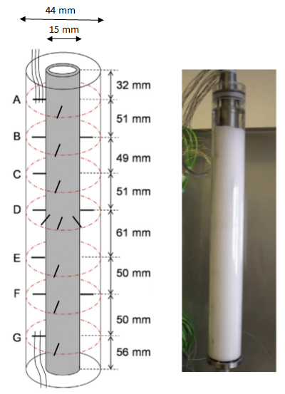
(a) Experimental setup by Longeon et al. [18]

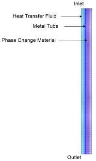
(b) Our computational domain and grid.

Figure 1: Simulation geometry based on the laboratory experiments of Longeon et al. [18]. Panel (a) shows their experimental setup, reprinted with their permission.

Details of the computational geometry are in Table 4(a). The structured grid used for the simulations is shown as Figure 1(b). The properties of the PCM, given in Table 4(c), are matched to those in Longeon et al. [18], with the exception of the sensible specific heat capacity and the density, which are different between the solid to liquid in the experiments but in the simulations are set to average values shown in Table 4(b). The properties of stainless steel in the simulations are density $8030\ kg/m^{3}$, specific heat capacity $502.48\ J/kgK$ and thermal conductivity of $16.27\ W/mK$.

(a) Geometry of simulation domain for validation

Parameter	Value	Unit
HTF tube
Outer Radius	10	mm
Inner Radius	7.5	mm
Length	400	mm
PCM container
Inner Radius	22	mm
Length	400	mm

(b) Properties of PCM used for simulation

Property	Value	Unit
$\rho$	820	$kg/m^{3}$
$L$	157	$kJ/kg$
$C_{p}$	2.1	$kJ/kg.K$
$\mu$	0.002706	$kg/m.s$
$\beta$	0.001	$1/K$
$T_{solidus}$	34.95	$\degree C$
$T_{liquidus}$	35	$\degree C$
$k$	0.2	$W/m.K$

(d) Properties of HTF Water

Property	Value	Unit
$\rho$	998.2	$kg/m^{3}$
$C_{p}$	4.182	$kJ/kg.K$
$\mu$	0.001003	$kg/m.s$
$k$	0.6	$W/m.K$

Table 4: Simulation parameters used in Longeon et al. [18]

.

(c) Properties of PCM RT35 Rubitherm as reported by [18]

Property	Value	Unit
$\rho$	880(s)/760(l)	$kg/m^{3}$
$L$	157	$kJ/kg$
$C_{p}$	1.8(s)/2.4(l)	$kJ/kg.K$
$\mu$	0.002706	$kg/m.s$
$\beta$	0.001	$1/K$
$T_{m}$	35	$\degree C$
$k$	0.2	$W/m.K$

4.1 Numerical details

The simulations are conducted using the finite volume code ANSYS Fluent. The simulation parameters are in Tables 4(b) and 4(d). In the phase-change model (4), the constant $A_{mush}$ defining the mushy zone is taken to be 100,000 and it is observed that the solution is not strongly dependent on this value.

The HTF inlet boundary condition is defined to be a uniform velocity of $0.01\ m/s$ and with static temperature 53$\degree$C. The HTF outlet boundary condition is constant gauge pressure of $0\ Pa$. The internal walls of the tube and PCM container are conjugate heat transfer internal boundaries with no slip. Heat transfer between the outer walls of PCM container and the room is ignored due to the low temperature differences between the heat transfer medium and ambient conditions. Thus, the outer walls are adiabatic with no slip. The vertical axis of the heat transfer fluid tube is defined to be a symmetry boundary condition so that the simulations are axisymmetric.

The mass and momentum equations are solved using the pressure based solver with the SIMPLE algorithm used for the pressure velocity coupling. Pressure is discretized using the PRESTO scheme [23]. The momentum and energy equations are discretized using second order upwind schemes. The evolution in time is first order implicit, as it is sufficient for most problems [1]. The solution is initialized with zero velocity in all directions and an ambient temperature of 23$\degree$C. The highest velocity in the domain is expected in the HTF and is twice the mean velocity, for a fully developed flow, which is $0.02\ m/s$.

4.2 Validation simulations

Sensitivity of the solutions to grid resolution and time step size are examined by varying the time step size by two orders of magnitude and the number of finite volumes in the grid by a factor of approximately eight. The important variable for energy storage is the melted fraction of the PCM, given as $\eta$. We perform simulations with grid sizes $3446$, $4696$ and $27996$ and time-step sizes of $0.1$ and $0.01$ seconds. Note that our smallest grid size and largest time-step are the same order of magnitude as the grid size of $9000$ and time-step of $0.5$ seconds used by Longeon et al. [18]. Figure 2 shows the melt fraction for the three grid sizes and two different time step ($\Delta t$) sizes. The results show that with increasing spatial and temporal resolution, the curves approach the results for the finest grid of $27996$ and the finest time-step size of $0.01$ seconds, and the difference between the intermediate resolution of $4696$ and $0.01$ seconds and the finest resolution is negligible. Table 5 shows the maximum of the absolute error(as percentage) in $\eta$ in reference to the finest resolution case, and we see that the error reduces by less than 1% beyond the intermediate resolution of $4696$ and $0.01$ seconds. Thus, the grid size of $4696$ nodes and a time step of $\Delta t=0.01$ seconds is sufficient to obtain grid insensitive results.

Figure 3 shows the comparison of temperature at a specific location D obtained from simulations and measured experimentally by Longeon et al. [18]. We see good agreement between the shapes of the experimental and numerical data curves.

Table 5: Grid sensitivity for melt fraction $\eta$, difference relative to nodes$=27996$ and $\Delta t=0.01$

$\eta$	Time Step (s)
Grid Size (nodes, cells)		0.1	0.01
	3446, 3170	2%	1%
	4696, 4356	1%	1%
	27996, 26733	1%	0

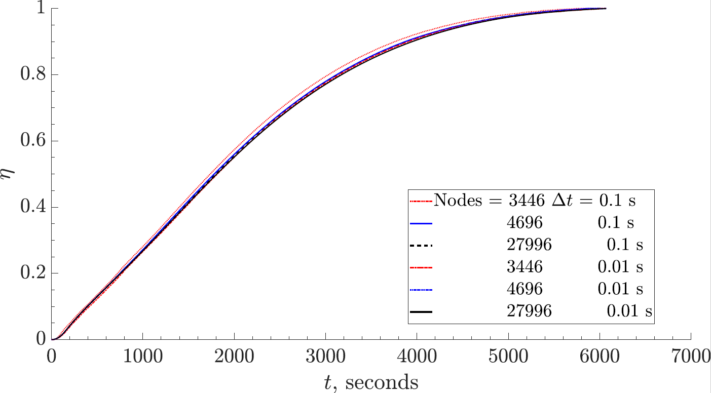
Figure 2: Grid Sensitivity, Average Melt Fraction in PCM

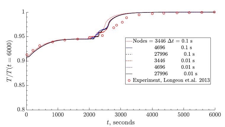
Figure 3: Comparison of measured temperature at Point D[18] with simulation for validating simulation procedure

4.3 Parametric study

Given the results of the validation experiments, we conclude that the simulation technique is adequate. After validating our simulation procedure, we proceeded to our parametric study. We vary the parameters $u_{f}$, $T_{in}$, $k_{p}$ and $k_{f}$ for the geometry and setup discussed in Longeon et al. [18], which we use for validating our simulations described in §4. $u_{f}$ is flow velocity for HTF and is the easiest to change through the use of a pump. $T_{in}$ is the inlet temperature of the HTF, which depends on the system from which we are extracting energy. $k_{p}$ and $k_{f}$ are dependent on material properties and additive enhancements and we have moderate control over them. Table 6 shows the endpoint values of parameters changed and table 7 shows the corresponding nominal dimensionless numbers.

Table 6: Physical parameters corresponding to values of dimensionless numbers in table 7. There are a total of 64 simulations created by varying each number in table 7 independently. For reasons of space, only the endpoint cases (numbering 16) have been shown here.

$u_{f}$	$k_{f}$	$k_{p}$	$T_{in}$	$Re_{f}$	$Pr_{f}$	$Pr_{p}$	$Gr_{p}$
0.01	0.1	0.1	310.125	149	42	57	24906
0.01	0.1	0.1	324.125	149	42	57	199248
0.01	0.1	1	310.125	149	42	6	24906
0.01	0.1	1	324.125	149	42	6	199248
0.01	0.8	0.1	310.125	149	5	57	24906
0.01	0.8	0.1	324.125	149	5	57	199248
0.01	0.8	1	310.125	149	5	6	24906
0.01	0.8	1	324.125	149	5	6	199248
0.14	0.1	0.1	310.125	2090	42	57	24906
0.14	0.1	0.1	324.125	2090	42	57	199248
0.14	0.1	1	310.125	2090	42	6	24906
0.14	0.1	1	324.125	2090	42	6	199248
0.14	0.8	0.1	310.125	2090	5	57	24906
0.14	0.8	0.1	324.125	2090	5	57	199248
0.14	0.8	1	310.125	2090	5	6	24906
0.14	0.8	1	324.125	2090	5	6	199248

Table 7: List of dimensionless numbers in parameter space and their values under study. Since the parameter space is four-dimensional, the total number of simulations are 64.

$Re_{f}$		$Pr_{f}$		$Pr_{p}$		$Gr_{p}$
$Re_{f}1$	149	$Pr_{f}1$	42	$Pr_{p}1$	57	$Gr_{p}1$	24906
$Re_{f}2$	2090	$Pr_{f}2$	5	$Pr_{p}2$	14	$Gr_{p}2$	83020
-	-	-	-	$Pr_{p}3$	8	$Gr_{p}3$	141134
-	-	-	-	$Pr_{p}4$	6	$Gr_{p}4$	199248

For example, for the four parameter case described here,

$$q_{pl}\ =q_{pl}\ (u_{f},k_{f},k_{p},T_{in})$$ (10)

The variable of interest is the stored energy, which is given by the time integral of $q_{pl}\$. Its dimensionless equivalent is $\eta$, the melt fraction, which we shall use henceforth for presenting results.

5 The structure of the melt fraction curve $\eta(t)$

In this section, we discuss some observations about the structure of $\eta$ prior to looking at the scaled results in section 6. We observed two distinct regions for $\eta$, specifically a linear and an asymptotic region, and name the melt fraction at the transition between these regions as the transition melt fraction denoted by $\eta_{critical}$ . The time at which $\eta_{critical}\$ occurs is denoted by $\tau_{critical}$; see section 6 for further discussion about obtaining a dimensionless time $\tau$ from $t$. We elaborate in §5.1 and §5.2 on why each region can be expected from physical reasoning.

5.1 Linear region

Based on Newton’s law of cooling, the heat transfer rate $q_{f}$ is set by the heat transfer coefficient $h_{f}$ and the temperature difference $T_{in}-T_{mci}$. Between the onset of melting and the transition melt fraction $\eta_{critical}$ , the temperature $T_{mci}$ is roughly constant due provided that transport of heat by the HTF does not limit the heat transfer into the PCM. If the variation is not significant compared to the total temperature difference $T_{in}-T_{mci}$, $T_{mci}$ and the difference can be considered to be constant. Indeed, for constant wall temperature with internal laminar flow, the non-dimensional heat transfer coefficient, which is the Nusselt number, is constant with value equal to 3.66 [13, eq. 8.55]. Thus, $q_{f}$ is expected to be a constant in this temperature region.

In the PCM, $q_{p}$ , which is comparable to $q_{f}$, is proportional to the temperature difference $T_{mci}-T_{mean}$, which is also constant. After an initial transient, $q_{pl}\$is the major component of $q_{p}$ . The melt fraction $\eta$, which is proportional to integral of $q_{pl}\$as shown in (2), is expected be linear with time. At $\eta_{critical}$ , the quantity of solid PCM gets small such that the characteristic temperature difference in the PCM is $T_{mci}-T_{p}$, where $T_{p}$ is the mean temperature of the PCM and is approximately equal to the far field temperature. $T_{p}$ is rising inverse-exponentially, which results in the asymptotic behavior of $\eta$, as explained in the following section.

5.2 Exponential region

Since the purpose of this section is to analze behavior rather than predicting data from first principles, we shall use simplified notation to obtain uncluttered equations. Terms expected to be constant have been grouped into numbered constants for brevity. Let the mass of solid PCM at the time $\eta$ reaches $\eta_{critical}$ be $m_{pcm}$, and let its surface area be $a_{pcm}$. Let the heat transfer coefficient on the solid liquid interface be $h_{pcm}$. Figure 4 shows a cartoon representation of the variables of interest.

After $\eta$ reaches a critical fraction $\eta_{critical}$ , the mass of solid PCM is small and the characteristic temperature difference is closer to $T_{mci}-T_{p}$ rather than $T_{mci}-T_{mean}$. The configuraton is shown in cartoon form in Figure 4 along with the notation used in the following discussion

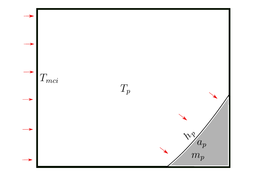
Figure 4: Cartoon figure showing the variables for the asymptotic model. The interface between $m_{pcm}$ and the liquid is an arbitrarily drawn curve.

In this regime, there is limited contact area between the liquid and the solid and so most of the heat transferred from the HTF to the PCM raises the temperature of the PCM. With this approximation,

$$q_{p}\ =M_{p}Cp_{p}\frac{dT_{p}}{dt} =h_{p}A_{p}(T_{mci}-T_{p})$$ (11)

$$\Rightarrow\frac{d(T_{mci}-T_{p})}{dt} =-\frac{h_{p}A_{p}}{M_{p}Cp_{p}}(T_{mci}-T_{p})$$

$$\Rightarrow\frac{d(T_{mci}-T_{p})}{T_{mci}-T_{p}} =-c_{2}^{\prime}dt$$

$$\Rightarrow ln(T_{mci}-T_{p}) =-c_{2}^{\prime}t+c_{1}$$

$$\Rightarrow T_{p} =T_{mci}-c_{2}e^{(-c_{2}^{\prime}t)}$$

In short, the PCM acts as a lumped capacitance Incropera et al. [13, eq. 5.8a] because the mass of the solid PCM is insufficient to affect $T_{p}$. Since the purpose of the foregoing is to arrive at the expected functional form rather than a numerically exact model, we have combined terms that are approximately constant into the coefficients the coefficients $c_{1}$, $c_{2}$, $c_{2}^{\prime}$. The prime notation denotes constants that carry forward into the final expression given in (14).

Assuming that the remaining solid PCM is at melting temperature and there is no significant sensible heating of the residual solid, the heat transfer to the solid PCM is

$$q_{pl}\ =L\frac{dm_{pcm}}{dt} =h_{pcm}A_{pcm}(T_{p}-T_{mean})$$ (12)

$$\Rightarrow\frac{d(1-\eta)}{dt} =\frac{h_{pcm}A_{pcm}}{LM_{p}}(T_{p}-T_{mean})\ .$$

The area $A_{pcm}$ depends on the mass of solid PCM and can be calculated if the the shape of $m_{pcm}$ and its density is known. Since the PCM is close to the melting temperature, the density can be considered to be a constant. At constant density, if $m_{pcm}$ is a sphere, $A_{pcm}$ is proportional to $m_{pcm}^{2/3}$. In general, $A_{pcm}$ is proportional to $m_{pcm}^{\gamma}$ where $\gamma$ is some real number less than 1, expected to be constant if the melting front geometry and density do not change in the duration of the exponential melting region. Substituting this and (11) into (12) yields

$$\frac{d(1-\eta)}{dt} =\frac{c_{3}h_{pcm}m_{pcm}^{p}}{LM_{p}}(T_{p}-T_{mean})$$ (13)

$$\Rightarrow\frac{d(1-\eta)}{dt} =\frac{c_{3}h_{pcm}(1-\eta)^{\gamma}}{LM_{p}^{1-\gamma}}(T_{p}-T_{mean})$$

$$\Rightarrow\frac{d(1-\eta)}{(1-\eta)^{\gamma}} =\frac{c_{3}h_{pcm}}{LM_{p}^{1-\gamma}}(T_{p}-T_{mean})dt$$

$$=c_{5}\left((T_{mci}-T_{mean})-c_{2}e^{(-c_{2}^{\prime}t)}\right)dt$$

$$=c_{5}(T_{mci}-T_{mean})dt-c_{2}c_{5}e^{(-c_{2}^{\prime}t)}dt$$

$$\Rightarrow\frac{(1-\eta)^{\gamma+1}}{\gamma+1} =c_{5}(T_{mci}-T_{mean})t+c_{6}e^{(-c_{2}^{\prime}t)}+c_{7}$$

$$\Rightarrow 1-\eta =\left(c_{7}^{\prime}+c_{5}^{\prime}(T_{mci}-T_{mean})t+c_{6}^{\prime}e^{(-c_{2}^{\prime}t)}\right)^{\frac{1}{\gamma+1}}$$

From this we conclude that the function form for $\eta(t)$ is

$$\eta=1-\left(c_{7}^{\prime}+c_{5}^{\prime}(T_{mci}-T_{mean})t+c_{6}^{\prime}e^{(-c_{2}^{\prime}t)}\right)^{\frac{1}{\gamma+1}}\ .$$ (14)

Again, we are interested in the form of the equation and the numbered coefficients collect constant terms that would make the form more difficult to read if included in full.

Figures 5 and 6 show the melt fraction and temperature contours when melting has reached $\eta_{critical}$ , for cases with different $Gr_{p}$ and $Pr_{p}$ values. The cases have vastly different operating parameters, but we can see that there are similarities in the melt fraction profiles, for example, the shape of the remaining PCM, which has been identified in §5.2 as a factor in determining the shape of the melt fraction curve. This suggests that $\eta_{critical}$ might be universal for a given device, at least in the range of dimensionless numbers studied.

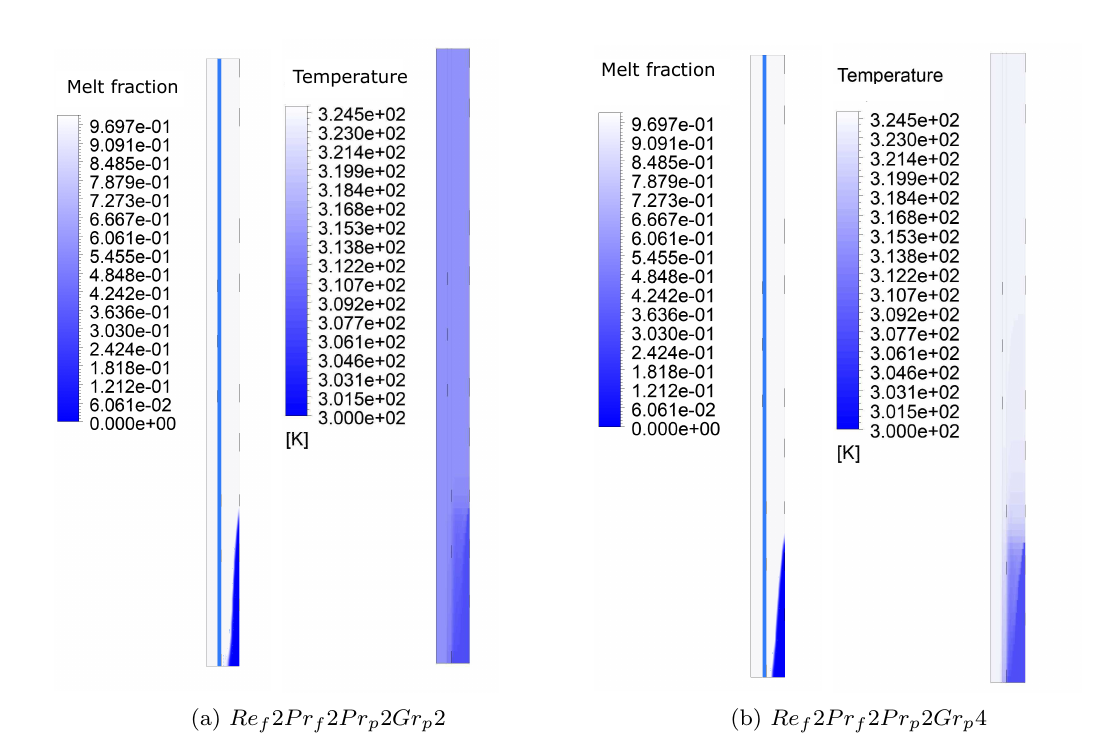
Figure 5: Plot of liquid fraction at time when $\eta_{critical}$ is reached for two Grashof numbers at $Re_{f}2$, $Pr_{f}2$ and $Pr_{p}2$. The corresponding temperature plot is shown to the right. Notice the similarity between the shape of the solid PCM for the two different cases. The figures are best viewed in conjunction with the geometry and grid shown in figure 1(b).

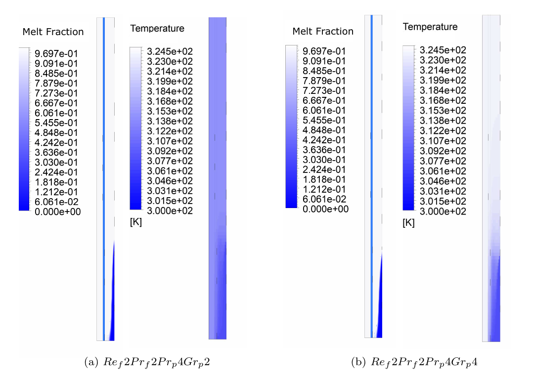
Figure 6: Plot of liquid fraction at time when $\eta_{critical}$ is reached for two Grashof numbers at $Re_{f}2$, $Pr_{f}2$ and $Pr_{p}4$. The corresponding temperature plot is shown to the right. Notice the similarity between the shape of the solid PCM for the two different cases and the cases from figure 5

From the arguments in §5.1 and §5.2, we expect $\eta$ to vary linearly in time when $\eta$ is small and to vary asymptotically with time when $\eta$ is large with the transition between the two regimes being $\eta_{critical}$ . This conclusion is based entirely on physical reasoning. In the following section, we apply this physical reasoning to the simulation data to understand the time evolution of $\eta$ and, in particular, how this time scales with the dimensional quantities in Table 1, and to determine the empirical value of $\eta_{critical}\$, which is of practical importance.

6 Application of methodology to understand flow physics

In the previous sections, we develop our approach for defining the dimensionless groups important for describing a simple LHTES systems such that they can be related to the heat transfer rate in a way consistent with the physical understanding developed from the theory of heat and mass transfer as well as the significant body of literature on LHTES systems. Here we demonstrate the utility of the approach by examining $\eta$ as a function of time in the multi-dimensional space defined $Gr_{p}$, $Pr_{p}$, $Re_{f}$ and $Pr_{f}$. The melt fraction $\eta$ has been defined previously as a function of dimensional time. For consistency, we denote the equivalent of $\eta$ that accepts a generic dimensionless time $\tau$ as an argument, by $\eta_{\tau}$. The goal is to find $\eta_{\tau}=\eta_{\tau}(\tau)$ with the $\tau$ defined in terms of a physically relevant time scale. If we are successful in this then the curves for $\eta_{\tau}(\tau)$ corresponding to different values of the parameter being varied will collapse to a single curve. In this section, we attempt to define a suitable $\tau$ based on the flow physics and observations from literature. As described in 2, we use the Buckingham-Pi theorem to organize our approach. A general dimensionless timescale can be defined as follows -

$$\tau=\tau(Fo_{p},Gr_{p},Pr_{p},Re_{f},Pr_{f})$$ (15)

where $Fo_{p}$ is the PCM Fourier number defined in table 3.

The simulation data base consists of 64 cases with parameters tabulated in Table 7. The simulations span a four-dimensional parameter space defined by $Re_{f}$, $Pr_{f}$, $Pr_{p}$ and $Gr_{p}$ with a high and low value for the first two and 4 values each for the rest. As mentioned in §5.1, we expect only a weak effect due to $Re_{f}$ and $Pr_{f}$, as long as there is sufficient heat flowing into the HTF domain. To confirm this, we perform additional simulations with two more intermediate values of $Re_{f}=796$ and $Re_{f}=1443$ at $Pr_{f}=42$, $Gr_{p}=8.302\times 10^{4}$ and $Pr_{p}=57$, the results of which are shown in figure 13. Similarly, we conduct simulations of two intermediate values of $Pr_{f}=8$ and $Pr_{f}=6$ for the case with $Re_{f}=2090$, $Pr_{p}=57$ and $Gr_{p}=8.302\times 10^{4}$, results of which are shown in figure 13. Given the expected and demonstrated weak effect of $Re_{f}$ and $Pr_{f}$, we fix their values and apply the methodology from §5, beginning with a cut through the parameter space along the plane defined by $Re_{f}=2090$ and $Pr_{f}=5$, that is, a particular set of HTF parameters. Based on the reasoning in §5 along with measurement data from the literature reviewed in §1, we expect time to scale with

$$\tau|_{Re_{f},Pr_{f}=constant}=Pr_{p}^{1/3}Gr_{p}Fo_{p}$$ (16)

for fixed $Re_{f}$ and $Pr_{f}$ indicated by the subscripts $Re_{f},Pr_{f}=constant$. For brevity, we also introduce a shorthand notation for a one dimensional slice through $\tau$, where all parameters except one are kept constant. For example, if all parameters except the PCM Grashof number $Gr_{p}$ were held constant, $\tau$ would be given as

$$\tau|_{Re_{f},Pr_{f},Pr_{p}=constant}(Gr_{p})=\tau_{pg}\$$ (17)

where the subscript $p$ denotes PCM and the additional subscript $g$ denotes that the Grashof number is the variable in question. To verify the hypothesis of (16), the data are plotted with this and other time scalings in Figure 7. In figure 13, it is observed that $Gr_{p}Fo_{p}$ collapses the data to a single curve provided that $Pr_{p}$ is constant but from figure 13 it is apparent that the collapse also occurs for multiple values of $Pr_{p}$. Similarly, figure 13 shows that $Pr_{p}^{1/3}Fo_{p}$ collapses the data to a single curve provided that $Gr_{p}$ is constant. These two relationships are combined in figure 7 and time is scaled according to (16) to collapse to almost a single curve all 16 cases having the same values for $Re_{f}$ and $Pr_{f}$.

A question that cannot be answered with the approach in §5 is the value of $\eta_{critical}$. This value is needed in order to inform whether the linear or asymptotic scaling of $\eta$ with time is appropriate. From observing figure 7, we estimate $\eta_{critical}\approx 0.9$. The existence of the linear and inverse-exponential regions is further supported by figure 14, which clearly shows the collapsed curves diverging as straight lines on the onset of the inverse-exponential region, as expected on a log-linear axes. Additionally, figures 13, 13 and 13 show that $\eta_{\tau}$ transitions to non-linear around $\eta_{critical}$ . We have noted in several places in this paper that the simulations are limited to laminar flow in the PCM whereas practical systems may employ turbulent flow. We know the reason, though, why the value of $\eta_{critical}$ will depend on the hydrodynamic regime of the PCM. In the remaining parts of this section, we discuss the scaling obtained and its practical implications.

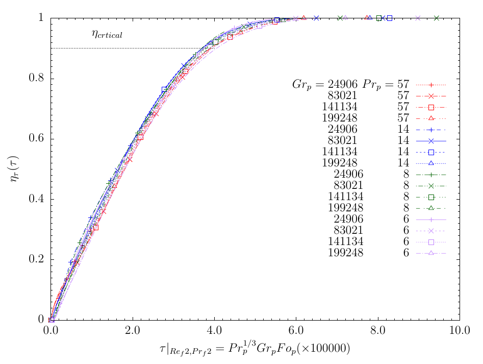
Figure 7: The melt fraction vs dimensionless time on the parameter plane with $Re_{f}=2090$ and $Pr_{f}=5$. All curves collapse, indicating that the timescale defined in (16) is appropriate if $Re_{f}$ is high enough and $Pr_{f}$ is low enough, or if $u_{f}$ and $k_{f}$ are both high enough to ensure sufficient heat flow. The markers are plotted to distinguish the curves.

6.1 Effects of $Gr_{p}$ and $Pr_{p}$: Discussion and implications

In this section, we discuss the reasons for the scaling obtained in figure 7 and the implications of this scaling for the design and operation of LHTES devices. Figures 13 and 13 shows plots for various cases from table 7 and we can see that the different cases collapse to one curve when the time is scaled with the PCM Grashof number, which agrees with our predictions in 5.1. This is consistent with what Jany and Bejan [14] observed by scaling analysis for mixed conduction-convection flow regimes in an enclosure with laminar flow. On reaching $\eta_{critical}$ , the curve changes shape from linear to asymptotic, as predicted in 5.2. In order to further confirm our hypothesis from 5.1, we plot the measured Grashof number in figure 13, which indicates that the PCM container wall temperature $T_{mci}$ is indeed constant for the cases under consideration. Figure 13 further confirms $Pr_{p}^{1/3}$ scaling obtained in figure 7. This scaling corresponds to the $Pr^{1/3}$ scaling observed in laminar forced convection with uniform heat flux. As explained in section 5.1, both the temperature difference $T_{mci}-T_{mean}$ and the heat transfer rate $q_{pl}\$are constant for majority of the time, as demonstrated by the linearity of the melt fraction curve. Due to the Boussinesq approximation, the simulated flow conserves volume, and a downward movement of volume must be matched by an upward movement. Thus, even though we cannot explain the scaling entirely, we note that the conditions in the PCM match those given in the analysis of Bejan [4, Eq 2.121], which predicts a $Pr^{1/3}$ dependency.

This implies that the temperature difference $T_{in}-T_{mean}$ is the most important parameter for obtaining fast heat transfer, and should be maximized. The HTF inlet temperature is constrained by the application being studied. Thus, the temperature difference may be maximized by picking a PCM with a lower mean melting temperature. However, increasing this difference corresponds to a loss in quality of heat stored. The temperature $T_{mean}$ is also expected to be an important parameter for heat transfer during discharging of the device, as it shall affect the discharging heat transfer rate. Thus, it is desirable to find an optimized value of $T_{mean}$ that maximizes the quality stored energy and the charging and discharging rates.

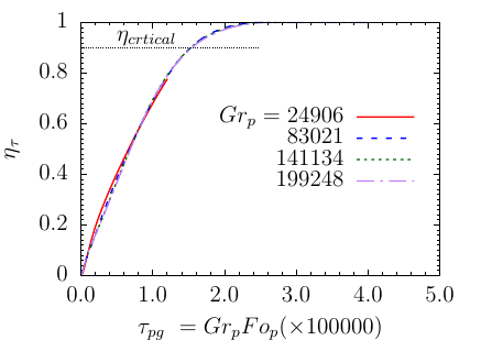
Figure 8: The scaling of melt fraction with the Grashof number on the parameter plane with $Re_{f}=2090$, $Pr_{f}=5$, $Pr_{p}=14$

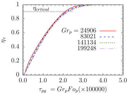
Figure 9: Analogous to figure 13, except $Pr_{p}=6$.

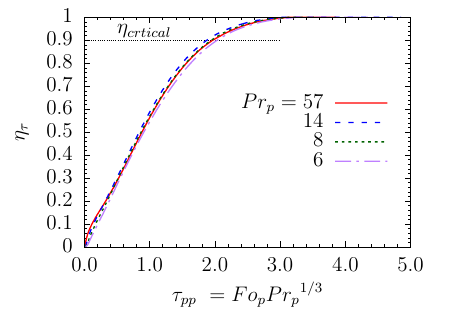
Figure 10: Melt Fraction $\eta$ as a function of $Pr_{p}$ at constant $Gr_{p}=199248$, $Pr_{f}=5$ and $Re_{f}=2090$. The figure shows the perfect scaling with ${Pr_{p}}^{1/3}$

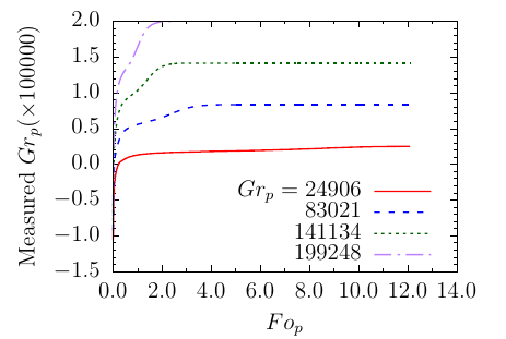
Figure 11: Measured $Gr_{p}$ as a function of non-dimensional time $\tau$, at constant $Re_{f}=2090$, $Pr_{f}=5$ and $Pr_{p}=6$. The plateau shows that the assumptions from §5.1 are justified. Negative Grashof numbers indicate that melting temperature has not been reached.

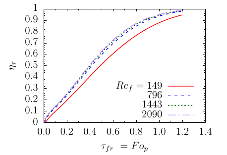
Figure 12: Melt Fraction as a function of $Re_{f}$ at constant $Gr_{p}=83020$, $Pr_{f}=42$ and $Pr_{p}=57$. The plots show that the heat transfer rate does not improve much past $Re=800$.

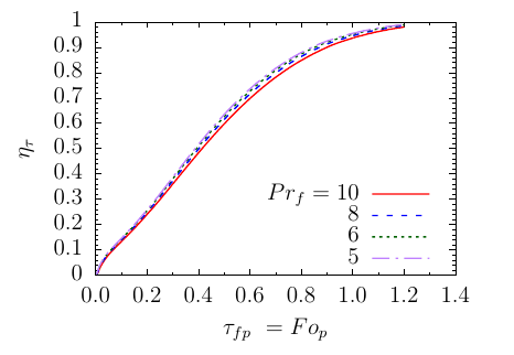
Figure 13: Melt Fraction as a function of four $Pr_{f}$ at constant $Gr_{p}=83020$, $Pr_{p}=57$ and $Re_{f}=2090$

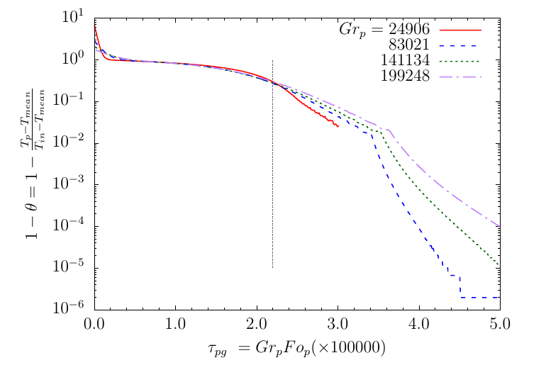
Figure 14: Dimensionless temperature plotted as $1-\theta$ at constant $Re_{f}=2090$, $Pr_{f}=5$ and $Pr_{p}=6$. The figure shows the existence of both linear and inverse-exponential regions as described in §5.1 and §5.2. The curves collapse in the linear region. They diverge at the onset of the inverse-exponential behavior, and are displayed as straight lines due to the log-linear axes.

6.2 Effects of $Re_{f}$ and $Pr_{f}$: Discussion and implications

Figure 13 shows $\eta_{\tau}$ for different values of $Re_{f}$. Increasing $Re_{f}$ reduces the boundary layer thickness in the HTF which increases $q_{f}$. We conclude that beyond $Re_{f}=800$, there is no significant improvement in $q_{f}$. Since the range of $Re_{f}$ presented here are in the laminar region, another possibility is that we would get further enhancement in $q_{f}$ with turbulent flow in the HTF pipe, which reduces the boundary layer thickness further. However, increasing the HTF thermal conductivity $k_{f}$ thus reducing the HTF Prandtl number $Pr_{f}$ also reduces the boundary layer thickness. Figure 13 shows that $q_{f}$ does not change significantly by increasing the thermal conductivity. This indicates that for the range of $Gr_{p}$ presented here, at $Re_{f}=800$, there is sufficient flow of energy into the HTF domain. Thus, it is desirable to maximize the energy available in the HTF region by selecting a HTF with sufficiently high conductivity and pumping it with sufficient velocity to remove the weak dependency of the heat transfer rate on $Re_{f}$ and $Pr_{f}$. As mentioned in §2, the fluid velocity is a parameter that can be easily controlled.

7 Conclusions

The parametric performance modeling of LHTES devices is essential for their effective use. In this paper, we present a framework to analyse LHTES devices and apply it to a typical shell and tube heat exchanger geometry. Out of all the parameters listed in table 1, we pick the fundamental operating parameters $u_{f}$,$T_{in}$ and two fundamental material parameters $k_{p}$,$k_{f}$ and study their effect on the heat transfer rate $q_{pl}\$and the melt fraction $\eta$ by conducting a matrix of 64 simulations. We observe that the melt fraction scales with the PCM Grashof number $Gr_{p}^{1}$ and the PCM Prandtl number $Pr_{p}^{(1/3)}$ provided that there is sufficient energy provided by the HTF. No significant scaling is observed for the HTF Reynolds number $Re_{f}$ and HTF Prandtl number $Pr_{f}$ in the range studied and we conclude that these parameters do not matter provided that the heat transfer rate is not limited by the HTF.

The form of $\eta$ versus time as the PCM melts has a linear region and a nonlinear region with the separation between them defined by a critical melt fraction $\eta_{critical}\ \approx 90\%$. The linear region is characterized by fast and constant heat transfer rate which is a desired characteristic in LHTES devices. The nonlinear region is characterized by an asymptotic approach to fully melted and a corresponding asymptotic decrease in the heat transfer rate. Contour plots of the liquid fraction at $\eta_{critical}$ for cases with vastly different parameters are observed to be similar in shape, which suggests a universality for the critical melt fraction $\eta_{critical}$ . Based on this, we make the following conclusions about the design process for LHTES devices that shall enable the maximization of heat transfer rates.

1. The HTF velocity and thermal conductivity have weak effects on the heat transfer rate, even at moderate values, provided that the HTF does not limit the overall availability of energy. As noted in §6, the velocity and the choice of HTF fluid are somewhat easier to customize than the PCM parameters, and the HTF velocity is limited only by considerations of optimizing pumping power and reducing pipe wear. This is termed as the ‘sufficient’ condition, and is indicated by the HTF tube walls approaching constant temperature. The values $Re_{f}=800$ and $Pr_{f}=8$ are found to be sufficient for the geometry studied here.

2. The variation of melt fraction $\eta$ (which is a measure of stored latent energy) with time consists of linear and asymptotic regions. The linear region is characterized by a constant and higher heat transfer rate, which makes it the relevant region for operating the heat exchanger as an energy storage device. The critical melt fraction $\eta_{critical}\$ denotes the transition between these regions, and the device should only be operated upto that value. For the current geometry, the value of $\eta_{critical}$ is 0.9.

3. Given ‘sufficient’ conditions in the HTF, the energy stored is given by the correlation $aPr_{p}^{1/3}Gr_{p}Fo_{p}$ where $a$ is a constant governed by the particular choice of geometry. This correlation, applicable in the linear region, can also stated as a dimensionless timescale given in (16).

4. The effect of the PCM Grashof number $Gr_{p}$ is much stronger than the PCM Prandtl number $Pr_{p}$. In terms of selecting PCM materials and operating parameters, this indicates that varying the melting point and/or HTF inlet temperature has a stronger effect on the heat transfer rate than enhancing the thermal conductivity of the PCM. However, if the charging and discharging HTF temperatures are fixed (this is expected, since they are governed by the application), increasing the charging $Gr_{p}$ reduces the discharging $Gr_{p}$. The melting point of the PCM should be optimized in order to satisfy both charging and discharging conditions. Hence, finding materials for which the melting point can be varied, with means such as additives or chemical composition, is indicated to be an important area for further research. This conclusion agrees with that of the the review presented by Farid et al. [10]

5. The HTF Prandtl number is a parameter that can be used to eliminate limiting HTF effects on heat transfer. Thus, enhancement of HTF conductivity through additives is indicated as a future research subject.

Acknowledgments

This work was sponsored by the US Department of Energy grants DE-EE00007708 and DE-EE00008277.

References

- ANSYS Fluent [2011] ANSYS Fluent. Fluent User Guide. In ANSYS FLUENT, volume 123, pages 407–408. 2011.
- Arbabzadeh et al. [2019] Maryam Arbabzadeh, Ramteen Sioshansi, Jeremiah X Johnson, and Gregory A Keoleian. The role of energy storage in deep decarbonization of electricity production in California. Nature Communications, (2019):1–35, 2019. ISSN 2041-1723.
- Bechiri, Mohammed and Mansouri, Kacem [2015] Bechiri, Mohammed and Mansouri, Kacem. Analytical solution of heat transfer in a shell-and-tube latent thermal energy storage system. Renewable Energy, 74:825–838, 2015. ISSN 09601481.
- Bejan [2013] Adrian Bejan. Convection Heat Transfer, Fourth Edition. 03 2013.
- Bhagat et al. [2018] Kunal Bhagat, Mohit Prabhakar, and Sandip K. Saha. Estimation of thermal performance and design optimization of finned multitube latent heat thermal energy storage. Journal of Energy Storage, 2018. ISSN 2352152X.
- Cao and Faghri [1991] Y Cao and A Faghri. Performance characteristics of a thermal energy storage module : a transient PCM/forced convection conjugate analysis. Int. J. Heat and Mass Transfer, pages 93–101, 1991.
- Cao and Faghri [1992] Y Cao and A Faghri. A Study of Thermal Energy Storage Systems With Conjugate Turbulent Forced Convection. Journal of Heat Transfer, pages 1019–1027, 1992.
- Denholm et al. [2010] P. Denholm, E. Ela, B. Kirby, and M. Milligan. Role of Energy Storage with Renewable Electricity Generation. Technical Report January, National Renewable Energy Laboratory, 2010.
- Diarce et al. [2018] G. Diarce, Campos-Celador, J. M. Sala, and A. García-Romero. A novel correlation for the direct determination of the discharging time of plate-based latent heat thermal energy storage systems. Applied Thermal Engineering, 129:521–534, 2018. ISSN 13594311.
- Farid et al. [2004] Mohammed M. Farid, Amar M. Khudhair, Siddique Ali K. Razack, and Said Al-Hallaj. A review on phase change energy storage: Materials and applications, 2004. ISSN 01968904.
- Gasia et al. [2017] Jaume Gasia, Jan Diriken, Malcolm Bourke, Johan Van Bael, and Luisa F. Cabeza. Comparative study of the thermal performance of four different shell-and-tube heat exchangers used as latent heat thermal energy storage systems. Renewable Energy, 2017. ISSN 18790682.
- Hu et al. [2017] Kang Hu, Lei Chen, Qun Chen, Xiao-Hai Wang, Jun Qi, Fei Xu, and Yong Min. Phase-change heat storage installation in combined heat and power plants for integration of renewable energy sources into power system. Energy, 124:640–651, 2017. ISSN 03605442.
- Incropera et al. [2011] Frank P Incropera, David P DeWitt, Adrienne S Lavine, and Theodore L Bergman. Fundamentals of heat and mass transfer. John Wiley & Sons, 2011.
- Jany and Bejan [1988] Peter Jany and Adrian Bejan. Scaling theory of melting with natural convection in an enclosure. International Journal of Heat and Mass Transfer, 31(6):1221–1235, 1988. ISSN 00179310.
- Johar et al. [2017] Dheeraj Kishor Johar, Dilip Sharma, Shyam Lal Soni, Pradeep K. Gupta, and Rahul Goyal. Experimental investigation and exergy analysis on thermal storage integrated micro-cogeneration system. Energy Conversion and Management, 131:127–134, 2017. ISSN 01968904.
- Kalapala and Devanuri [2018] Lokesh Kalapala and Jaya Krishna Devanuri. Influence of operational and design parameters on the performance of a pcm based heat exchanger for thermal energy storage – a review. Journal of Energy Storage, 20:497 – 519, 2018. ISSN 2352-152X.
- Li et al. [2017] Jun Li, Chin Hong Tam, and Guohong Tian. Investigation of an HD Engine Thermal Storage System. Energy Procedia, 105(0):4110–4115, 2017. ISSN 18766102.
- Longeon et al. [2013] Martin Longeon, Adèle Soupart, Jean François Fourmigué, Arnaud Bruch, and Philippe Marty. Experimental and numerical study of annular PCM storage in the presence of natural convection. Applied Energy, 2013. ISSN 03062619.
- McDaniel and Kosanovic [2016] Benjamin McDaniel and Dragoljub Kosanovic. Modeling of combined heat and power plant performance with seasonal thermal energy storage. Journal of Energy Storage, 7:13–23, 2016.
- Mongibello et al. [2014] L. Mongibello, M. Capezzuto, and G. Graditi. Technical and cost analyses of two different heat storage systems for residential micro-CHP plants. Applied Thermal Engineering, 71(2):636–642, 2014. ISSN 13594311.
- Nithyanandam and Pitchumani [2013] K. Nithyanandam and R. Pitchumani. Computational Modeling of Dynamic Response of a Latent Thermal Energy Storage System With Embedded Heat Pipes. Journal of Solar Energy Engineering, 2013. ISSN 0199-6231.
- Rathod and Jyotirmay [2015] K. Rathod and Banerjee Jyotirmay. Development of Correlation for Melting Time of Phase Change Material in Latent Heat Storage Unit. In Energy Procedia, pages 2125–2130, 2015. ISBN 1876-6102.
- Shmueli et al. [2010] H. Shmueli, G. Ziskind, and R. Letan. Melting in a vertical cylindrical tube: Numerical investigation and comparison with experiments. International Journal of Heat and Mass Transfer, 2010. ISSN 00179310.
- Teamah et al. [2016] Hebat-Allah M. Teamah, Marilyn F. Lightstone, and James S. Cotton. Numerical Investigation and Nondimensional Analysis of the Dynamic Performance of a Thermal Energy Storage System Containing Phase Change Materials and Liquid Water. Journal of Solar Energy Engineering, 2016. ISSN 0199-6231.
- Venkitaraj et al. [2018] K. P. Venkitaraj, S. Suresh, and Arjun Venugopal. Experimental study on the thermal performance of nano enhanced pentaerythritol in IC engine exhaust heat recovery application. Applied Thermal Engineering, 137(October 2017):461–474, 2018. ISSN 13594311.
- Voller and Prakash [1987] V. R. Voller and C. Prakash. A fixed grid numerical modelling methodology for convection-diffusion mushy region phase-change problems. International Journal of Heat and Mass Transfer, 1987. ISSN 00179310.
- Yimer and Adami [1997] B. Yimer and M. Adami. Parametric study of phase change thermal energy storage systems for space application. Energy Conversion and Management, 38(3):253–262, feb 1997. ISSN 0196-8904.