A robust Lyapunov criterion for non-oscillatory behaviors in biological interaction networks

Abstract

We introduce the notion of non-oscillation, propose a constructive method for its robust verification, and study its application to biological interaction networks (also known as, chemical reaction networks). We begin by revisiting Muldowney’s result on the non-existence of periodic solutions based on the study of the variational system of the second additive compound of the Jacobian of a nonlinear system. We show that exponential stability of the latter rules out limit cycles, quasi-periodic solutions, and broad classes of oscillatory behavior. We focus then on nonlinear equations arising in biological interaction networks with general kinetics, and we show that the dynamics of the aforementioned variational system can be embedded in a linear differential inclusion. We then propose algorithms for constructing piecewise linear Lyapunov functions to certify global robust non-oscillatory behavior. Finally, we apply our techniques to study several regulated enzymatic cycles where available methods are not able to provide any information about their qualitative global behavior.
Keywords: second additive compounds, robust non-oscillation, piecewise linear Lyapunov functions, biological interaction networks, enzymatic cycles.

I Introduction

Natural and engineered nonlinear systems are commonly required to operate consistently and robustly under perturbations and a variety of environmental conditions. Rational analysis and synthesis of such systems need qualitative characterizations of their global long-term behavior, which is a notoriously difficult task for general nonlinear systems. This problem is compounded by the large uncertainties that pervade the mathematical descriptions of many such systems. A prominent class exemplifying these difficulties are biological interaction networks, which include molecular processes such as expression and decay of proteins, metabolic networks, regulation of transcription and translation, and signal transduction [1]. Such networks are usually described via the mathematical formalism of Biological Interaction Networks (BINs) (also known as Chemical Reaction Networks (CRNs)) [2]. Ordinary Differential Equations (ODE) descriptions of BINs have two components, one graphical and one kinetic. The first is often well-characterized as it corresponds to the list of reactions, while the latter (which includes kinetic constants and the functional forms of kinetics) is not, as it depends on quantifying the “speed” of reactions which is difficult to measure and subject to environmental changes. This information disparity precludes the construction of full mathematical models, and hence a pressing need has emerged for the development of general robust techniques that can provide conclusions on the qualitative behavior of the network based on the graphical information only [3].

Although this problem may seem intractable, significant progress has been made in the past few decades. A pioneering example has been the development of the theory of complex-balanced networks with Mass-Action kinetics, and the associated deficiency-based characterizations [4, 5]. It has been shown that such networks always admit Lyapunov functions over the positive orthant, and that global stability can be ascertained in some cases [6, 7]. Other notions of global behavior have also been considered in the literature. It has been shown that the persistence of a class of BINs can be certified via simple graphical conditions [8]. The monotonicity of certain BINs can be established in reaction coordinates, and this property has been used to show global convergence to attractors [9]. More recently, new techniques have been developed for certifying global stability by the construction of Robust Lyapunov Functions (RLFs) in reaction coordinates [10, 11, 12] and concentration coordinates [13, 12, 14, 15]. These techniques have been developed into a comprehensive framework with relatively wide applicability to various key biochemical networks like transcriptional networks, post-translational modification cascades, signal transduction, etc [12].

Despite recent advances, many relevant networks, and many dynamic behaviors, remain outside the scope of analysis through available methods. In this paper, we study oscillations in dynamical systems with particular emphasis on BINs. Unlike earlier works which studied conditions for the emergence of oscillations in various physical contexts [16, 17], we propose to study another global qualitative notion, which we call non-oscillation, by examining the variational system of the second additive compound of the Jacobian of a nonlinear system. This approach was originally introduced in order to rule out periodic solutions by Muldowney [18] (see also [19], where the approach has recently been reframed in the context of $k$-Order Contraction Theory), and it has been applied to the study of epidemic models [20], circadian rhythms [21], and, most remarkably, as a local analysis tool, [22], to rule out Hopf bifurcations in BINs. We begin by revisiting Muldowney’s results. We will show that exponential stability of the aforementioned variational system guarantees that the area measure of all bidimensional compact surfaces asymptotically converges to zero. It turns out, as a consequence, that the same will be true of the $k$th-hypervolume measure for arbitrary $k$-dimensional submanifolds for any $k\geq 2$. This allows us to exclude limit cycles, invariant torii, (asymptotically) quasi-periodic solutions, and many types of oscillatory behavior. We then show that this notion can be verified successfully for classes of BINs where no other technique has proved useful. We will achieve this goal by embedding the dynamics of the second additive compounds of a BIN in a linear differential inclusion, and then generalize the RLF approach to be applied to this LDI. We will show that the existence of such an RLF will guarantee robust non-oscillation by establishing a LaSalle-like condition.

Although robust non-oscillation is technically weaker than global stability, coupling it with local asymptotic stability is nearly as good as it places robust and strong constraints on the range of possible behaviors of a given network. Furthermore, this new notion is also compatible with multi-stability and almost global stability [23, 24], which opens the door for applications to systems with multiple attractors.

I-A Motivating example: regulation of the enzymatic cycle

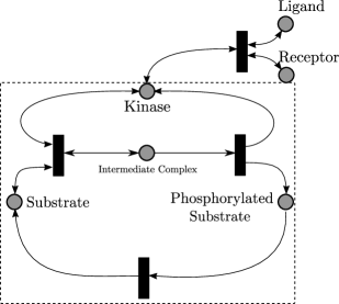
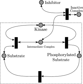
Figure 1: Various architectures for regulating the PTM cycle. (a) The kinase is only activated if a ligand binds to a receptor, (b) The kinase gets deactivated after binding to an inhibitor, (c) The substrate-kinase intermediate complex gets sequestered by an inhibitor. The Petri-net [25] notation is used where a circle denotes a species, and a rectangle denotes a reaction.

We describe an open problem which is highly relevant to systems biology. It involves regulation mechanisms of the Post-Translational Modification (PTM) cycle which is a very common motif in signal transduction [26]. For example, an enzyme known as a kinase ($K$) binds to a substrate ($S$) to form an intermediate complex ($C$). Then, the substrate is phosphorylated to produce an activated substrate ($P$). The activated substrate decays back to its inactive form ($S$). The network is depicted inside the dashed rectangle in Figure 1-a)-c), and it can be written as follows:

$$S+K\rightleftharpoons C\longrightarrow P+K,\ P\longrightarrow S.$$ (1)

The dynamics of the above network has been analyzed using a Piecewise Linear (PWL) RLF. In particular, it has been shown that it always admits a positive globally asymptotic stable steady state, for any choice of monotone kinetics [11, 12].

However, small structural changes in the network can make a PWL RLF fail to exist. We study various ways of regulating the activity of the cycle as depicted in Figure 1. In one scenario, the kinase can only be activated if two molecules bind (e.g, a ligand ($L$) and a receptor ($Rc$)) as shown in Figure 1-a. This is modelled by adding the reaction

$${Rc}+L\rightleftharpoons K$$ (2)

to the BIN (1). It can be shown that this network has a unique positive steady steady state for each assignment of non-zero total substrate, ligand and receptor concentrations [27, 28]. However, a PWL RLF fails to exist [29, 12]. It has been shown recently that this network enjoys local asymptotic stability for any choice of kinetics, i.e., the Jacobian matrix is always Hurwitz at any steady state [30]. However, there are no known robust global guarantees on the asymptotic behavior. Other regulation mechanisms exist [28]. For instance, the kinase might be inactivated by binding to an inhibitor ($I$) such as a drug used in targeted cancer therapies [31]. This is represented by adding the reaction $K+I\rightleftharpoons EI$ to the network (1) as shown in Figure 1-b). A third possible architecture has the intermediate complex ($C$) sequestered by $I$. Hence, the reaction $C+I\rightleftharpoons CI$ is added to (1). None of these networks can be globally analyzed using current techniques. We will be studying these networks under our new framework and show that they are globally non-oscillatory.

It is worth mentioning that not all regulation mechanisms of the PTM are beyond current methods of analysis. For instance, instead of a simple decay of $P$ to $S$, another enzyme called a phosphatase can be used to accelerate the dephosphorylation of $P$ back to $S$. This latter architecture is well-studied [9], and its global stability can be certified by a PWL RLF [12].

This paper is organized as follows. Mathematical definitions and notation are given in section II. Section III revisits Muldowney’s results in terms of exponential stability. Section 4 provides a robust Lyapunov criterion for robust non-oscillation when the dynamics can be embedded in a Linear Differential Inclusion (LDI). Section 5 studies the application of the results to BINs. Section 6 provides algorithms for constructing the PWL RLF. Section 7 studies several examples of enzymatic cycles that have not been amenable to methods in the literature. Finally, section 8 is dedicated to a brief discussion of the results.

II Non-oscillatory systems

II-A Definitions and Notation

Our basic concepts and results are not restricted to BINs, but apply to more general classes of nonlinear systems. For a dynamical system

$$\dot{x}(t)=f(x(t)),$$ (3)

with the state $x:\mathbb{R}_{\geq 0}\to\mathbb{R}^{n}$ and $f:X\subset\mathbb{R}^{n}\rightarrow\mathbb{R}^{n}$ of class $\mathcal{C}^{1}$, we denote by $\varphi(t,x_{0})$ the solution at time $t$ from initial condition $x_{0}$ at time $0$. Moreover, $\omega(x_{0})$ denotes the $\omega$-limit set of such a solution. The set $X$ can be arbitrary, but we assume that it is forward invariant for the dynamics, that is, $\varphi(t,x_{0})\in X$ for all $t\geq 0$ and all $x_{0}\in X$. Class $\mathcal{C}^{1}$ means that $f$ is the restriction of a $\mathcal{C}^{1}$ function defined on some open neighborhood of $X$. We let $\mathbb{D}:=\{z\in\mathbb{R}^{2}:z_{1}^{2}+z_{2}^{2}\leq 1\}\subset\mathbb{R}^{2}$ denote the unit disk, $\mathbb{S}:=\{[\cos(\theta),\sin(\theta)],\theta\in[0,2\pi]\}$ the unit circle, and $\mathbb{S}^{k}$ the $k$-dimensional torus.

Definition 1.

We say that (3) exhibits oscillatory behavior if, for some integer $k\geq 1$, it admits a compact invariant set $\Omega\subset{X}$ which is the image of a $\mathcal{C}^{1}$ injection $h:\mathbb{S}^{k}\rightarrow X$ not everywhere singular. If it does not admit such a set then we say that (3) is non-oscillatory.

Notice that Definition 1 includes systems with many kind s of non-converging behavior, in particular, systems with periodic solutions, or asymptotically periodic solutions. In this case $\omega(x_{0})$ is invariant and diffeomorphic to $\mathbb{S}$. Furthermore, it includes systems with multiple incommensurable oscillation frequencies, (such as quasiperiodic solutions, or asymptotically quasiperiodic solutions). In such a case $\omega(x_{0})$ is the image of $\mathbb{S}^{k}$, for some $k>1$ and some map $h$. It also includes other types of non-convergent behaviors, such as solutions approaching a closed curve of equilibria, and certain types of homoclinic and heteroclinic orbits (of finite length). Moreover, it also encompasses certain types of chaotic systems as the associated attractors are sometimes known to embed unstable periodic solutions [32].

While the gap between non-convergent and oscillatory behavior seems to be extremely small in practice, ruling out its existence appears to be very challenging, given the existing technical tools.

We introduce some of the required background on compound matrices and their role in assessing the evolution of $k$-hypervolumes along solutions of a dynamical system. For an arbitrary $\mathcal{C}^{1}$ injection $h:\mathbb{D}\rightarrow X\subset\mathbb{R}^{n}$, the area of $h(\mathbb{D})$ can be computed as:

$$\mu_{2}(h(\mathbb{D})):=\int_{\mathbb{D}}\sqrt{\sum_{I\subset\{1,\ldots,n\}:|I|=2}\left[\textrm{det}\left(\frac{\partial h_{I}}{\partial z}(z)\right)\right]^{2}}\,dz_{1}dz_{2}.$$ (4)

where, for a set $I=\{i_{1},i_{2},\ldots,i_{|I|}\}\subset\{1,2,\ldots n\}$ with elements ordered according to $i_{1}<i_{2}<\ldots<i_{|I|}$, and a vector $h$, $h_{I}$ denotes the sub-vector $[h_{i_{1}},h_{i_{2}},\ldots,h_{i_{|I|}}]^{\prime}$. Similarly, for any given $\mathcal{C}^{1}$ injective map $h:\mathbb{S}^{k}\rightarrow\mathbb{R}^{n}$, and $k\geq 1$, the $k$-hypervolume of $h(\mathbb{S}^{k})$ can be obtained according to:

$$\mu_{k}(h(\mathbb{S}^{k}))$$ (5)

$$:={\Huge\int_{\mathbb{S}^{k}}}\sqrt{\sum_{I\subset\{1,\ldots,n\}:|I|=k}\left[\textrm{det}\left(\frac{\partial h_{I}}{\partial\theta}(\theta)\right)\right]^{2}}\,d\theta_{1}d\theta_{2}\ldots d\theta_{k}.$$

These quantities can further be defined along solutions of (3); in particular, we aim at quantifying $\mu_{2}(\varphi(t,h(\mathbb{D})))$ and $\mu_{k}(\varphi(t,h(\mathbb{S}^{k})))$. To this end, we associate to system (3) the family of variational equations:

$$\begin{array}[]{rcl}\dot{x}&=&f(x)\\ \dot{\delta}^{(k)}(t)&=&{\dfrac{\partial f}{\partial x}^{(k)}(x(t))}\normalsize\,\delta^{(k)}(t)\end{array}$$ (6)

where $\delta^{(k)}$ is a vector in $\mathbb{R}^{{n\choose k}}$ and, for any $A\in\mathbb{R}^{n\times n}$, $A^{(k)}\in\mathbb{R}^{{n\choose k}\times{n\choose k}}$ denotes the $k$-th additive compound matrices for $k=1\ldots n$, which are defined element-wise as follows [18]:

$$A_{IJ}^{(k)}=\left\{\begin{array}[]{ll}A_{i_{1}i_{1}}+...+A_{i_{k}i_{k}},&\mbox{if}~{}I=J\\ (-1)^{\ell+s}A_{i_{s}j_{\ell}},&\mbox{if exactly one entry}~{}i_{s}~{}\mbox{of}~{}I\\ &\mbox{does not occur in}~{}J\\ &\mbox{and}~{}j_{\ell}~{}\mbox{does not occur in}~{}I\\ 0,&\mbox{if}~{}I~{}\mbox{differs from}~{}J~{}\mbox{in two}\\ &\mbox{ or more entries},\end{array}\right.$$ (7)

where $I,J\subset\{1,..,n\}$ are of cardinality $k$, respectively denoted as $I=\{i_{1},i_{2},\ldots,i_{k}\}$, $J=\{j_{1},j_{2},\ldots,j_{k}\}$ with entries indexed such that $1\leq i_{1}<i_{2}<...<i_{k}\leq n$ and $1\leq j_{1}<j_{2}<\ldots<j_{k}\leq n$.

To exemplify this construction, consider the case $k=2$, which will later be our main object of study, and the $4\times 4$ matrix, $A=[a_{ij}]$. The corresponding $6\times 6$ additive compound matrix $A^{(2)}$ reads:

$$\left(\begin{array}[]{cccccc}a_{11}+a_{22}&a_{23}&a_{24}&-a_{13}&-a_{14}&0\\ \\ a_{32}&a_{11}+a_{33}&a_{34}&a_{12}&0&-a_{14}\\ \\ a_{42}&a_{43}&a_{11}+a_{44}&0&a_{12}&a_{13}\\ \\ -a_{31}&a_{21}&0&a_{22}+a_{33}&a_{34}&-a_{24}\\ \\ -a_{41}&0&a_{21}&a_{43}&a_{22}+a_{44}&a_{23}\\ \\ 0&-a_{41}&a_{31}&-a_{42}&a_{32}&a_{33}+a_{44}\end{array}\right).$$

Fix any subset $J\subset\{1,2,\ldots,n\}$ of cardinality $k$. It is known [18] that, by arranging minors of $\partial\varphi/\partial x_{J}$ for all subsets $I\subset\{1,2,\ldots,n\}$ of cardinality $k$ in lexicographic order within the vector $\delta^{(k)}(t)$ as follows

$$\delta^{(k)}(t):=\left[\begin{array}[]{c}\vdots\\ \textrm{det}\left(\frac{\partial\varphi_{I}}{\partial x_{J}}(t,x)\right)\\ \vdots\end{array}\right],$$ (8)

the resulting vector $\delta^{(k)}(t)$ fulfills the $k$-th variational equation (6) with initial condition $x(0)=x$ and

$$\delta^{(k)}(0)=\left[\begin{array}[]{c}\vdots\\ \delta_{I,J}\\ \vdots\end{array}\right],$$

where $\delta_{I,J}:=1$ iff $J=I$ and $0$ otherwise. These properties will be exploited in subsequent sections to quantify how the hypervolumes previously defined evolve along solutions of the considered system of differential equations.

II-B Muldowney’s result revisited

Our main goal for this section is to obtain an analog to Muldowney’s result [18] by making use of the notion of uniform exponential stability. His seminal paper shows that if the logarithmic norm of the second-additive compound of the Jacobian matrix is negative throughout state-space for a nonlinear system, (non-trivial) periodic solutions cannot exist. We formulate the result by using the notion of uniform exponential stability of the associated second-additive compound variational equation, so that we can verify assumptions and certify properties through the construction of suitable Lyapunov functions for an associated LDI. Moreover, we strengthen the original result by generalising its applicability to invariant submanifolds of any dimension. We start with the following Lemma about time varying-matrices:

Lemma 1.

Let $\Lambda(t):\mathbb{R}_{\geq 0}\to\mathbb{R}^{n\times n}$ be a time-varying matrix. If all minors of order $k$ of $\Lambda(t)$ converge to $0$ so do all minors of order $q\geq k$. Furthermore, if the assumed convergence is exponential, then so is the convergence of all minors of order $q\geq k$.

Proof.

We prove the result by induction, by showing that if the convergence happens for $k$, then it is also fulfilled for $q=k+1$.

Recall that for an invertible square matrix $A$ of dimension $q$, it holds that $A\,\textrm{adj}(A)=\textrm{det}(A)I_{q}$, where $\textrm{adj}(A)$ denotes the adjoint matrix of $A$. Hence, taking determinants in both sides of this previous equality we get:

$$\textrm{det}(A)\cdot\textrm{det}(\textrm{adj}(A)) =\textrm{det}(A\,\textrm{adj}(A))$$

$$=\textrm{det}(\textrm{det}(A)I_{q})=\textrm{det}(A)^{q}.$$

In particular then, $\textrm{det}(\textrm{adj}(A))=\textrm{det}(A)^{q-1}$. Taking absolute values and inverting this relationship yields:

$$|\textrm{det}(A)|=\psi(\textrm{adj}(A))$$ (9)

where $\psi:\mathbb{R}^{n\times n}\to\mathbb{R}_{\geq 0}$ is continuous and given as $\psi(B)=\sqrt[q-1]{|\textrm{det}(B)|}$. Note that $\psi(0)=0$. More generally, if $A$ is singular, then $\mbox{det}(A)=0$ means also that the inequality trivially holds:

$$|\textrm{det}(A)|\leq\psi(\textrm{adj}(A)).$$ (10)

We will apply this observation to the matrices $A=[\Lambda]_{IJ}$ for any choice of $I,J\subset\{1,2,\ldots,n\}$ of cardinality $q$. By the induction hypothesis for any $\tilde{I}$,$\tilde{J}$ of cardinality $k$ it holds,

$$\lim_{t\rightarrow+\infty}\textrm{det}\left([\Lambda]_{\tilde{I}{\tilde{J}}}(t)\right)=0.$$

Hence, the same is true of each of the entry of the adjoint matrix (which by definition are minors of dimension $q-1=k$ possibly multiplied by $-1$):

$$\lim_{t\rightarrow+\infty}\textrm{adj}\left([\Lambda]_{{I}{{J}}}(t)\right)=0.$$

In particular, then, our convergence claim follows from (10) and continuity of $\psi$ and the fact that $\psi(0)=0$.

In order to prove exponential convergence, assume that for some $M$ and $\lambda>0$, the following is true:

$$\textrm{det}\left([\Lambda]_{\tilde{I}{\tilde{J}}}(t)\right)\leq Me^{-\lambda t}\qquad\forall\,t\geq 0$$

for all $\tilde{I}$, $\tilde{J}$ of cardinality $k$. We see that for all $I$, $J$ of cardinality $k+1$, and all $i,j$ in $\{1,\ldots,k+1\}$, it holds that:

$$\left|\textrm{adj}\left([\Lambda_{IJ}](t)\right)_{i,j}\right|\leq Me^{-\lambda t}\qquad\forall\,t\geq 0.$$

Hence, substituting the above entry-wise upper-bound in (10) yields:

$$|\mbox{det}\left([\Lambda_{IJ}](t)\right)| \leq\psi\left(\textrm{adj}\left([\Lambda_{IJ}](t)\right)\right)$$

$$\leq\sqrt[k]{(k+1)!M^{k+1}e^{-(k+1)\lambda t}}=\tilde{M}e^{-\frac{k+1}{k}\lambda t}$$

for a suitable choice of $\tilde{M}$. This completes the proof of the induction step in the case of exponential convergence. ∎

The following corollary follows:

Corollary 1.

Assume that for some initial condition $x(0)=x$ and some $k\in\{1,2,\ldots n\}$, the solutions of (6) with arbitrary initial conditions $\delta^{(k)}(0)\in\mathbb{R}^{{n\choose k}}$ fulfil:

$$\lim_{t\rightarrow+\infty}\delta^{(k)}(t)=0.$$

Then, the same is true for all solutions $\delta^{(q)}(t)$ of (6) for $q$ in $\{k,k+1,\ldots,n\}$. Moreover, if the assumed convergence to $0$ is exponential (and uniform), so is it for $\delta^{(q)}(t)$.

Proof.

The result follows from the previous Lemma because of the connection between solutions of (6) and minors of $\frac{\partial\varphi}{\partial x}(t,x)$ for any given initial condition $x_{0}$. Hence, the claim is equivalent to showing that if all minors of order $k$ of $\Lambda(t):=\frac{\partial\varphi}{\partial x}(t,x)$ converge (exponentially) to $0$ so do all minors of order $k+1$. The latter statement immediately follows from the previous Lemma. ∎

Our main Theorem for general systems is as follows.

Theorem 1.

Consider a dynamical system as in (3):

$$\dot{x}(t)=f(x(t)),$$ (11)

and assume that, for some convex set $K$ and all $x_{0}\in K\subset X$, the second variational equation

$${\dot{\delta^{(2)}}(t)=\frac{\partial f}{\partial x}^{(2)}(x(t))\,\delta^{(2)}(t)}$$ (12)

is uniformly exponentially stable, i.e., there exist $M,\lambda>0$ such that, for all $t\geq 0$ and all $\delta^{(2)}(0)$:

$$|\delta^{(2)}(t)|\leq Me^{-\lambda t}\,|\delta^{(2)}(0)|,$$ (13)

with $M$ and $\lambda$ independent of $x(0)$ and $\delta^{(2)}(0)$. Then, the dynamical system (3) is non-oscillatory.

Proof.

The statement can be proved by contradiction. We start for the sake of simplicity, from the case $k=2$. Assume $h$ be a $\mathcal{C}^{1}$ function $h:\mathbb{S}^{2}\rightarrow K$, not everywhere singular, such that $h(\mathbb{S}^{2})\subset K$ is invariant. Of course, since $\varphi(t,h(\mathbb{S}^{2}))=h(\mathbb{S}^{2})$ by definition of invariant set:

$$\mu_{2}(\varphi(t,h(\mathbb{S}^{2})))=\mu_{2}(h(\mathbb{S}^{2}))>0,$$ (14)

where the last inequality follows by the implicit function theorem given that $h$ is not everywhere singular. On the other hand,

$$\mu_{2}(\varphi(t,h(\mathbb{S}^{2})))=$$ (15)

$${\Huge\int_{\mathbb{S}^{2}}}\sqrt{\sum_{I\subset\{1,\ldots,n\}:|I|=2}\left[\textrm{det}\left(\frac{\partial}{\partial\theta}\varphi_{I}(t,h(\theta))\right)\right]^{2}}\,d\theta_{1}d\theta_{2}.$$

Moreover, by the chain rule,

$$\frac{\partial}{\partial\theta}\varphi_{I}(t,h(\theta))=\frac{\partial}{\partial x}\varphi_{I}(t,h(\theta))\frac{\partial h}{\partial\theta},$$

and therefore by the Cauchy-Binet formula:

$$\textrm{det}\left(\frac{\partial}{\partial\theta}\varphi_{I}(t,h(\theta))\right)$$

$$=\sum_{J\subset{1,\ldots,n}:|J|=2}\textrm{det}\left(\frac{\partial}{\partial x_{J}}\varphi_{I}(t,h(\theta))\right)\textrm{det}\left(\frac{\partial h_{J}}{\partial\theta}\right)$$

$$=\sum_{J\subset{1,\ldots,n}:|J|=2}\delta_{I}^{(2)}(t,[h(\theta),e_{J}])\cdot\textrm{det}\left(\frac{\partial h_{J}}{\partial\theta}\right).$$

where $\delta^{(2)}(t,[x_{0},\delta_{0}^{(2)}])$ denotes the $\delta^{(2)}$-component of the solution of (12) from initial conditions $x(0)=x_{0}$ and $\delta^{(2)}(0)=\delta_{0}^{(2)}$. We may therefore seek to bound from above the integrand (15) using:

$$\textrm{det}\left(\frac{\partial}{\partial\theta}\varphi_{I}(t,h(\theta))\right)^{2}$$

$$\leq 2\sum_{J\subset{1,\ldots,n}:|J|=2}\left[\delta_{I}^{(2)}(t,[h(\theta),e_{J}])\right]^{2}\cdot\textrm{det}\left(\frac{\partial h_{J}}{\partial\theta}\right)^{2}.$$

Taking sums over $I$ we get:

$$\sum_{I\subset\{1,\ldots,n\}:|I|=2}\left[\textrm{det}\left(\frac{\partial}{\partial\theta}\varphi_{I}(t,h(\theta))\right)\right]^{2}$$

$$\leq 2\sum_{I,J\subset{1,\ldots,n}:|I|,|J|=2}\left[\delta_{I}^{(2)}(t,[h(\theta),e_{J}])\right]^{2}\cdot\left[\textrm{det}\left(\frac{\partial h_{J}}{\partial\theta}\right)\right]^{2}$$

$$=2\sum_{J\subset{1,\ldots,n}:|J|=2}\left|\delta^{(2)}(t,[h(\theta),e_{J}])\right|^{2}\cdot\left[\textrm{det}\left(\frac{\partial h_{J}}{\partial\theta}\right)\right]^{2}.$$

Moreover, by exponential uniform stability of (12) we see that:

$$\mu_{2}(\varphi(t,h(\mathbb{S}^{2})))$$

$$\leq\int_{\mathbb{S}^{2}}\sqrt{2\sum_{J\subset{1,\ldots,n}:|J|=2}M^{2}e^{-2\lambda t}\cdot\textrm{det}\left(\frac{\partial h_{J}}{\partial\theta}\right)^{2}}d\theta_{1}d\theta_{2}$$

$$=\sqrt{2}Me^{-\lambda t}\mu_{2}(h(\mathbb{S}^{2})).$$

The latter inequality however contradicts (14) for all $t$ sufficiently large. An analogous proof applies to any invariant set which is the image of an injection $h$ of $\mathbb{S}^{k}$ for $k>2$, thanks to Corollary 1. Notice that convexity of $K$ was not crucial so far in the proof.

We consider next the case $k=1$. Let $h:\mathbb{S}\rightarrow K$ be a class $\mathcal{C}^{1}$ map such that $h(\mathbb{S})$ is invariant. Pick any point $\tilde{x}\in K$. We consider the map $\tilde{h}:\mathbb{D}\rightarrow K$ defined as $\tilde{h}(z):=(1-|z|)\tilde{x}+|z|h(z/|z|)$ (this is a convex combination of $\tilde{x}$ and points of $h(\mathbb{S})$ and it therefore belongs to $K$ by convexity of the set). By construction $\tilde{h}$ defines a surface (not necessarily smooth everywhere) such that $\tilde{h}(\partial\mathbb{D})=h(\mathbb{S})$. Notice that, by invariance of $h(\mathbb{S})$ this is also true of the map $\varphi(t,\tilde{h}(\cdot))$, i.e., $\varphi(t,\tilde{h}(\partial\mathbb{D}))=h(\mathbb{S})$. Our goal is to estimate the area of $\varphi(t,\tilde{h}(\mathbb{D}))$. This can be computed according to:

$$\mu_{2}(\varphi(t,\tilde{h}(\mathbb{D})))$$ (16)

$$={\Huge\int_{\mathbb{D}}}\sqrt{\sum_{I\subset\{1,\ldots,n\}:|I|=2}\left[\textrm{det}\left(\frac{\partial}{\partial z}\varphi_{I}(t,\tilde{h}(z))\right)\right]^{2}}\,dz_{1}dz_{2}.$$

Following the same steps as in the previous proof we see that:

$$\mu_{2}(\varphi(t,\tilde{h}(\mathbb{D})))\leq\sqrt{2}Me^{-\lambda t}\mu_{2}(\tilde{h}(\mathbb{D})).$$ (17)

However, by [33], there exists a surface of minimal area which is bounded by a given contour. This surface may, in general, present self-intersections depending on how complex is the contour (for instance due to the presence of knots). Moreover, the surface of minimal area has positive measure $\underline{\mu}>0$, [33, 18]. This, however contradicts (17) for all sufficiently large $t>0$. This concludes the proof of the Theorem. ∎

Remark 1.

We point out that replacing second additive compound matrices in (12) with the standard Jacobians, that is the case of $k=1$ instead of $k=2$, yields classical variational criteria for exponential incremental stability. Theorem 1 hence relaxes such assumptions since, by virtue of Corollary 1, exponential convergence for $k=1$ (as needed in incremental stability) implies exponential convergence for all higher values of $k$. The converse is obviously not true.
It is worth pointing out that condition (13), in combination with the other assumptions of Theorem 1, is only a sufficient condition for ruling out oscillatory behaviors. In the case of constant matrices the second additive compound is asymptotically stable iff the real part of the sum of the dominant and subdominant eigenvalues is negative. This affords existence of an unstable eigenvalue, provided the subdominant one is sufficiently within the left-hand side of the complex plane. Likewise, in a time-varying context, one can expect exponential stability as in (13) provided the dominant and subdominant Lyapunov exponents have negative sum.

Remark 2.

Notice that our conditions are also independent of so called Dual Lyapunov functions, as introduced by Rantzer, [34]. Specifically Rantzer makes use of the derivative of $n$-forms along the flow in order to impose an expansion condition on the volume everywhere away from the equilibrium of interest. This implies almost global convergence to the equilibrium under suitable integrability conditions on the considered density functions.

III Robust Lyapunov criterion for persistently-excited differential inclusions

In our subsequent treatment of BINs, we are interested in studying notions of robust non-oscillation. We interpret “robustness” in the control theory sense of structured uncertainties. Hence, we study a class of uncertain dynamical systems. Given the dynamical system (12), we want to study the case in which the dynamics of $\delta^{(2)}(t)$ can be embedded in a Linear Differential Inclusion (LDI). For simplicity, we denote $z(t):=\delta^{(2)}(t)$.

III-A Common Lyapunov functions for LDIs

Similar to our previous works [13, 12], we seek to find a convex PWL Lyapunov function $V:\mathbb{R}^{N}\rightarrow\mathbb{R}_{\geq 0}$ of the following form:

$$V(z)=\max_{k\in\{1,\ldots,L\}}c_{k}^{T}z,$$ (18)

for some vectors $c_{1},\ldots,c_{L}\in\mathbb{R}^{N}$, where $N:={n\choose 2}$ to be evaluated for $z(t)=\delta^{(2)}(t)$ as defined in (6).

We state the following definition :

Definition 2.

Let the matrices $A_{1},..,A_{s}\in\mathbb{R}^{N\times N}$, and a locally Lipschitz function $V:\mathbb{R}^{N}\to\mathbb{R}_{\geq 0}$ be given. For each $\varepsilon\geq 0$ let $\mathcal{A}_{\varepsilon}$ denote the set:

$$\mathcal{A}_{\varepsilon}=\left\{\sum_{\ell=1}^{s}\alpha_{\ell}A_{\ell}:\alpha_{\ell}\geq\varepsilon,\ell=1\ldots s\right\}.$$ (19)

Then, we say that $V$ is a common non-strict Lyapunov function for the LDI

$$\dot{z}(t)\in\mathcal{A}_{\varepsilon}z(t)$$ (20)

if $V(z)$ is positive definite, (that is $V(z)>0$ for all $z\neq 0$) and it satisfies $\nabla V(z)Az\leq 0$ whenever $\nabla V(z)$ exists and for all $A\in\mathcal{A}_{\varepsilon}$.

Remark 3.

We show in Lemma 9 in the Appendix that the conditions given in Definition 2 are necessary and sufficient for the time-derivative of $V$ (defined as the upper Dini’s derivative) to be non-positive when evaluated over an arbitrary trajectory of the LDI. The details are given in the Appendix.

The following characterization is standard, but we include a proof in the Appendix to make the discussion self-contained.

Lemma 2.

Let the matrices $A_{1},..,A_{s}$, and a locally Lipschitz function $V:\mathbb{R}^{N}\to\mathbb{R}_{\geq 0}$ be given. Then, $V$ is a common Lyapunov function for the LDI (20) iff $V$ is positive definite and

$$V(e^{{A}t}z)\leq V(z),\qquad\forall\,z,\forall\,t\geq 0,\;\forall\,A\in\mathcal{A}_{\varepsilon}.$$ (21)

III-B Asymptotic stability and LaSalle’s argument

Notice that the individual subsystems only need to fulfill the non-strict inequality (21) which implies Lyapunov stability, and not asymptotic stability. In order to prove uniform exponential stability of a differential inclusion on the basis of existence of a non-strict Lyapunov function, we need a LaSalle-like criterion in conjunction with some notion of persistence of excitation. For this purpose, we will prove asymptotic stability of the differential inclusion (20) for every $\varepsilon>0$. We refer to (20) as a Persistently-Excited LDI (PELDI). Notice that,

$$\mathcal{A}_{\varepsilon}\subsetneq\mathcal{A}_{0}=\textrm{cone}\left\{A_{1},A_{2},\ldots,A_{s}\right\},$$

where “cone” denotes conic hull.

Intuitively speaking this system is persistently excited since every vertex of the nominal differential inclusion (achieved for $\varepsilon=0$) takes part (at least with some $\varepsilon$ contribution) to the formation of the state derivative direction. This arises naturally in the context of BINs since a topology-based criteria based on the absence of critical siphons is sufficient to prove non-extinction of all chemical species (a property known also as persistence [8]) and this leads to a potentially tighter embedding as in (20).

Hence, for a given LDI (20) and the associated PWL Lyapunov function $V(z)$, we define the matrices given below:

$$M_{i}:=[A_{1}^{T}c_{i},A_{2}^{T}c_{i},\ldots,A_{s}^{T}c_{i}],$$ (22)

for all $i\in\{1,2\ldots L\}$.

Our main result for this section is stated below.

Theorem 2.

Let $V(z)$ be a PWL common Lyapunov function for system (20) with $\varepsilon=0$. Assume that

$$\textrm{Ker}[M_{i}^{T}]=\{0\},\qquad\forall\,i\in\{1,2,\ldots,L\}.$$ (23)

Then, for all $\varepsilon>0$ the PELDI (20) is uniformly exponentially stable.

Proof.

Fix any $\varepsilon>0$ and let $x(t)$ be an arbitrary solution of (20). Since $V$ is a common Lyapunov function for (20) with $\varepsilon=0$ it is a fortiori a common Lyapunov function for (20) because of the inclusion $\mathcal{A}_{\varepsilon}\subset\mathcal{A}_{0}$. Hence, $V(x(t))\leq V(x(0))$ for all $t\geq 0$. Hence $x(t)$ is bounded (by positive definiteness and radial unboundedness of $V$). The Lyapunov function $V(x(t))$ is non-increasing along $x(t)$ and therefore it admits a limit as $t\rightarrow+\infty$. Let $\bar{v}\geq 0$ be the value of this limit. The solution $x(t)$ approaches its non-empty $\omega$-limit set $\omega(x(\cdot))$ and $V(\bar{x})=\bar{v}$ for all $\bar{x}\in\omega(x(\cdot))$. The set $\omega(x(\cdot))$ is weakly invariant, [35]. We pick an arbitrary solution $\tilde{x}(t)$ of (20) such that $\tilde{x}(t)\in\omega(x(\cdot))$ for all $t\geq 0$. For each $t\geq 0$ we consider the set of active vectors:

$$\mathcal{C}(t):=\{k:V(\tilde{x}(t))=c_{k}^{T}\tilde{x}(t)\}.$$ (24)

and define the corresponding set-valued map, $\mathcal{C}:t\mapsto 2^{\{1,\ldots,L\}}$. By continuity of $\tilde{x}(t)$ the set-valued map $\mathcal{C}$ is upper-semicontinuous, viz. for any $t$ and any open neighborhood $U$ of $\mathcal{C}(t)$ there exists a neighborhood $N_{t}$ of $t$ such that $\mathcal{C}(N_{t})\subset U$. Hence, since $\mathcal{C}$ only takes discrete values, we see that the above inclusion can be strengthened to $\mathcal{C}(N_{t})\subset\mathcal{C}(t)$. Letting $t$ be a point where the cardinality of $\mathcal{C}(t)$ is minimal (which exists by finiteness of the set $\{1,2,\ldots,L\}$) we see that $\mathcal{C}(N_{t})=\mathcal{C}(t)$ and therefore there exists an interval $[t,\tilde{t}]$ ($\tilde{t}>t$) where $\mathcal{C}(\tau)=\mathcal{C}(t)$ for all $\tau\in[t,\tilde{t}]$. Pick any $k\in\mathcal{C}(t)$. We know that $V(\tilde{x}(\tau))=c_{k}^{T}\tilde{x}(\tau)=\bar{v}$ for all $\tau$ in the considered interval. Hence, by definition of solution of (20):

$$c_{k}^{T}\dot{\tilde{x}}(\tau)=c_{k}^{T}\sum_{\ell=1}^{s}\alpha_{\ell}(\tau)A_{\ell}\tilde{x}(\tau)=\sum_{\ell=1}^{s}\alpha_{\ell}(\tau)c_{k}^{T}A_{\ell}\tilde{x}(\tau)=0$$

for some $\alpha_{\ell}(\tau)\geq\varepsilon$, and almost all $\tau\in[t,\tilde{t}]$. Recalling that $c_{k}^{T}A_{\ell}\tilde{x}(\tau)\leq 0$, and using continuity of $\tilde{x}(\tau)$ this in turn implies:

$$c_{k}^{T}A_{\ell}\tilde{x}(\tau)=0,\qquad\forall\,\ell\in\{1,2,\ldots,L\}\;\forall\tau\in[t,\tilde{t}].$$

Hence, $\tilde{x}(\tau)$ belongs to $\textrm{Ker}[M_{k}^{T}]$, and by assumption (23) $\tilde{x}(\tau)=0$. By strong invariance of the origin, this implies $\omega(x(\cdot))=\{0\}$ and therefore (see e.g. Theorem 2 in [36]) uniform exponential stability of (20) for all $\varepsilon>0$ follows, by a standard relaxation argument.

∎

Remark 4.

Conditions (23) are used to rule out, using a first order derivative test, existence of non-zero solutions of (20) evolving on a level-set of $V$ for some time-interval. As such, they could be relaxed by formulating higher order differential tests. This, however, would increase significantly the complexity of their verification. Such relaxation was not needed in practical examples.

Remark 5.

It is shown in [15] that a BIN admitting a non-strict polyhedral Lyapunov function is asymptotically stable iff a robust non-singularity condition (for strictly positive linear combinations) holds on the matrices defining the embedding of the nonlinear differential equation. Theorem (2) differs in several respects.
It is, in fact, a stability result for a linear differential inclusion, rather than for nonlinear dynamics which are embedded within a linear differential inclusion. Notice also that the matrices $M_{i}$ in (22) both involve the Lyapunov function vectors $c_{i}$ and the dynamics of the switched system. As such, condition (23) is not immediately related to a condition of robust non-singularity which, by definition, only involves the matrices of the switched system. We cannot rule out that, on a deeper level, condition (23) might be related or even equivalent to a robust non-singularity test.

IV Robust non-oscillation of BINs

In this section we study non-oscillation of BINs as described in §2.

IV-A Background on BINs

We use the standard notation [2, 5, 12]. A BIN (also called a “Chemical Reaction Network”) is a pair $(\mathcal{S},\mathcal{R})$ with a set of admissible kinetics $\mathscr{K}_{\mathcal{S},\mathcal{R}}$ to be defined below.

Stoichiometry

The finite set of species is denoted by $\mathcal{S}:=\{S_{1},S_{2},\ldots,S_{n_{s}}\}$, which combine and transform through a finite set of reactions, $\mathcal{R}:=\{{\mathrm{R}}_{1},{\mathrm{R}}_{2},\ldots,{\mathrm{R}}_{n_{r}}\}$. A non-negative linear integer combination of species is called a complex, and an ordered pair of complexes define a reaction which is written customarily as:

$${\mathrm{R}}_{j}:\sum_{i=1}^{n_{s}}\alpha_{ij}S_{i}\rightarrow\sum_{i=1}^{n_{s}}\beta_{ij}S_{i},$$

with integer coefficients $\alpha_{ij},\beta_{ij}$ (called the stoichiometry coefficients). These are usually arranged in a matrix $[\Gamma]_{ij}:=\beta_{ij}-\alpha_{ij}$, called the stoichiometry matrix, whose $(i,j)$-entry specifies the net amount of molecules of $S_{i}$ produced or consumed by reaction ${\mathrm{R}}_{j}$. If $\sum_{i=1}^{n_{s}}\beta_{ij}S_{i}\rightarrow\sum_{i=1}^{n_{s}}\alpha_{ij}S_{i}$ is also a reaction, then we say that ${\mathrm{R}}_{j}$ is reversible and we write $\sum_{i=1}^{n_{s}}\alpha_{ij}S_{i}\rightleftharpoons\sum_{i=1}^{n_{s}}\beta_{ij}S_{i}$.

Kinetics

The kinetics of the BIN can be defined by introducing a non-negative state vector $x=[x_{1},x_{2},\ldots,x_{n_{s}}]^{T}$ quantifying the concentration of each species and a choice of kinetics, i.e., a functional expression for the rates at which the corresponding reaction takes place: ${R(\cdot)}:\mathbb{R}_{\geq 0}^{n_{s}}\rightarrow\mathbb{R}_{\geq 0}^{n_{r}}.$ The function $R(\cdot)$ can take many forms, and we assume that it satisfies basic smoothness and monotonicity requirements defined as follows:

1. $R_{j}(x)$ is continuously differentiable, $j=1,..,n_{r}$;

2. if $\alpha_{ij}>0$, then $x_{i}=0$ implies $R_{j}(x)=0$;

3. ${\partial R_{j}}/{\partial x_{i}}(x)\geq 0$ if $\alpha_{ij}>0$ and ${\partial R_{j}}/{\partial x_{i}}(x)\equiv 0$ if $\alpha_{ij}=0$;

4. The inequality in A3 holds strictly for all positive concentrations, i.e when $x\in\mathbb{R}_{+}^{n}$.

Condition A2 represents the fact that a reaction cannot occur when any of its reactants is missing. Conditions A3 and A4 require that, at least in the interior of the positive orthant, rates be strictly monotone functions of reactants’ concentrations. Furthermore, A3 specifies that only reactants can influence the rate of any reaction. If a reaction rate $R$ satisfies A1-4 we say that it is admissible. The set of all admissible reaction rates of a given BIN $(\mathcal{S},\mathcal{R})$ is denoted by $\mathscr{K}_{\mathcal{S},\mathcal{R}}$.

A typical choice of kinetics are the so called Mass-Action kinetics, which correspond to the following polynomial expression:

$$R_{j}(x)=k_{j}\prod_{i=1}^{n_{s}}x_{i}^{\alpha_{ij}},$$ (25)

for some constant parameter $k_{j}>0$ and with the convention that $a^{0}=1$ for all $a\in\mathbb{R}$.

Dynamics

the dynamical system associated to the BIN is by definition:

$$\dot{x}=\Gamma R(x).$$ (26)

This is a (generally) nonlinear, positive system, meaning that solutions have non-negative coordinates given that the initial conditions do. For each initial condition $x_{0}$, the affine space $\mathcal{C}_{x_{0}}=x_{0}+\textrm{Im}[\Gamma]$ is so that the corresponding solution $\varphi(t,x_{0})$ belongs to $\mathcal{C}_{x_{0}}$ for all $t\geq 0$, i.e., $\mathcal{C}_{x_{0}}$ is forward invariant. Hence, the system dimension is often reduced by taking into account an independent set of conservation laws (viz. vectors in $\textrm{Ker}(\Gamma^{T})$) and regarding the flow induced by (26) as parametrized by the total amount of each conservation law, and evolving on a lower dimensional space defined by the corresponding stoichiometry class. This is the approach that we will pursue also throughout this paper. In particular, we will choose a basis for $\textrm{Ker}(\Gamma^{T})$ (assumed of dimension $c$) as $\{v_{1},v_{2},\ldots,v_{c}\}$ and complete it to a basis of $\mathbb{R}^{n}$, $\{v_{1},v_{2},\ldots v_{c},v_{c+1},\ldots,v_{n}\}$ so that, defining the matrix:

$$T=[v_{1},v_{2},\ldots,v_{n}]^{T}$$

we may define the system in $\tilde{x}$ coordinates according to $\tilde{x}=Tx$. Accordingly the new equations read:

$$\dot{\tilde{x}}=T\Gamma R(T^{-1}\tilde{x})=\left[\begin{array}[]{c}0_{n_{c}}\\ \Gamma_{r}R(T^{-1}\tilde{x})\end{array}\right],$$ (27)

where $\Gamma_{r}=[v_{c+1},\ldots,v_{n}]^{T}\Gamma$ is a reduced stoichiometry matrix. Of course, the natural state-space in $\tilde{x}$ coordinates, (i.e., $T\mathbb{R}_{\geq 0}^{n}$) is not necessarily the positive orthant, but possibly a subset of it (as the individual vectors $v_{i}$, $i=1,\ldots,n$ are often chosen to be non-negative). Notice that, the vector $\tilde{x}$ can be partitioned according to $[\tilde{x}_{c},\tilde{x}_{d}]$ where $\tilde{x}_{c}$ corresponds to the first $c$ components of $\tilde{x}$ (which are constant along solutions) while $\tilde{x}_{d}$ corresponds to the remaining $n-c$ coordinates evolving according to non-trivial dynamics.

Siphons

Since (26) evolves on the positive orthant, certain trajectories might approach the boundary of the orthant asymptotically, i.e., some species might go extinct. If no species becomes extinct for every positive initial state, then the dynamical system is said to be persistent. In order to characterize persistence graphically, we need some definitions. Let $P\subset\mathcal{S}$ be a nonempty set of species. A reaction ${\mathrm{R}}_{j}\in\mathcal{R}$ is said to be an input reaction to $P$ if there exists $S_{i}\in P$ such that $\beta_{ij}>0$, while a reaction ${\mathrm{R}}_{j}\in\mathcal{R}$ is said to be an output reaction to $P$ if there exists $S_{i}\in P$ such that $\alpha_{ij}>0$. Then, the set $P$ is called a siphon if each input reaction associated to $P$ is also an output reaction associated to $P$ [8]. The species that correspond to the support of a non-negative conservation law automatically constitute a siphon. Hence, any siphon that contains the support of a conservation law is said to be trivial. If a siphon is not trivial, then it is said to be critical. If a BIN has no critical siphons, then (26) is persistent for any choice of monotone kinetics [8].

Graphical representation

A BIN can be represented as a graph in various ways. We adopt the Petri-net representation [25, 8], which is also equivalent to a species-reaction graph [28]. For a given BIN, species correspond to places, while reactions correspond to transitions. The incidence matrix of the Petri-net is simply the stoichiometry matrix $\Gamma$. An example will be discussed next.

Example

Referring to the motivational example (1)-(2), the reactions are ordered as:

$$L+{Rc}\xrightleftharpoons[{\mathrm{R}}_{2}]{{\mathrm{R}}_{1}}K,\ S+K\xrightleftharpoons[{\mathrm{R}}_{4}]{{\mathrm{R}}_{3}}C\mathop{\longrightarrow}\limits^{{\mathrm{R}}_{5}}P+K,\ P\mathop{\longrightarrow}\limits^{{\mathrm{R}}_{6}}S.$$ (28)

The concentrations $x_{1},..,x_{6}$ correspond to the species $L,{Rc},K,S,C,P$, respectively. The ODE can be written as:

$$\dot{x}=\left[\begin{array}[]{rrrrrr}-1&1&0&0&0&0\\ -1&1&0&0&0&0\\ 1&-1&-1&1&0&0\\ 0&0&-1&1&1&1\\ 0&0&1&-1&-1&0\\ 0&0&0&0&1&-1\end{array}\right]\left[\begin{array}[]{l}R_{1}(x_{1},x_{2})\\ R_{2}(x_{3})\\ R_{3}(x_{3},x_{4})\\ R_{4}(x_{5})\\ R_{5}(x_{5})\\ R_{6}(x_{6})\end{array}\right]$$ (29)

where the rates $R_{j},j=1,..,6$ satisfy the Assumptions A1-4. Beyond these assumptions we don’t assume that anything is known about them. The Petri-net graph of the network is depicted in Figure 1-a).

The BIN (28) has three conserved quantities which are the total receptor, the total ligand, and the total substrate. The corresponding conservation laws can be written as: $x_{1}+x_{3}+x_{5}=x_{1,tot}$, $x_{2}+x_{3}+x_{5}=x_{2,tot}$, $x_{4}+x_{5}+x_{6}=x_{3,tot}$. Note that the network has no critical siphons and hence it is persistent. The conservation laws can be used to reduce the equation above from a six-dimensional to a three-dimensional ODE. For instance, we can choose the independent variables to be $x_{1},x_{3},x_{6}$ (corresponding to $L,K,P$). Hence $T$ can be written as:

$$T=\begin{bmatrix}1&0&1&0&1&0\\ 0&1&1&0&1&0\\ 0&0&0&1&1&1\\ 1&0&0&0&0&0\\ 0&0&1&0&0&0\\ 0&0&0&0&0&1\end{bmatrix}.$$ (30)

For given total positive conserved quantities $x_{1,tot},x_{2,tot},x_{4,tot}>0$, we obtain in this manner an ODE for the evolution of $\tilde{x}_{d}(t)=[x_{1},x_{3},x_{6}]^{T}(t)$, as follows:

$$\dot{\tilde{x}}_{d}=\left[\begin{array}[]{rrrrrr}-1&1&0&0&0&0\\ 1&-1&-1&1&0&0\\ 0&0&0&0&1&-1\end{array}\right]R({\tilde{x}}_{d}),$$ (31)

where

$$R({\tilde{x}}_{d})=\left[\begin{array}[]{l}R_{1}(x_{1},x_{1}-x_{1,tot}+x_{2,tot})\\ R_{2}(x_{3})\\ R_{3}(x_{3},x_{4,tot}-x_{1,tot}+x_{1}+x_{3}-x_{6})\\ R_{4}(x_{1,tot}-x_{1}-x_{3})\\ R_{5}(x_{1,tot}-x_{1}-x_{3})\\ R_{6}(x_{6})\end{array}\right].$$

While, as is well known, this change of coordinates conveniently achieves a dimensionality reduction of the underlying dynamics, it plays a crucial role in enabling the analysis of BINs by using second additive compound matrices. This is so because structural zero eigenvalues of the Jacobian are removed, opening up the possibility of establishing uniform exponential convergence of the associated variational equations.

IV-B Lyapunov criteria for robust non-oscillation of BINs

We apply the concept of non-oscillation to BINs. Since the reaction rates are not assumed to be known beyond satisfying assumptions A1-4, we aim at establishing a notion of robust non-oscillation.

Definition 3.

Let a BIN $(\mathcal{S},\mathcal{R})$ be given. We say that it is robustly non-oscillatory if the associated dynamical system (26) is non-oscillatory for every choice of kinetics $R\in\mathscr{K}_{\mathcal{S},\mathcal{R}}$.

We aim at proving the non-oscillatory nature of the dynamics by embedding the variational equation associated to the second additive compound matrix within a linear differential inclusion. This is reminiscent of our approach for treating robust global stability for BINs [13],[12]. To this end, take the Jacobian of the $\tilde{x}$-dynamics (27), as the principal submatrix of indices $\{c+1,\ldots n\}$:

$$J_{r}(\tilde{x})=\left[T\Gamma\frac{\partial R}{\partial x}T^{-1}\right]_{c+1,\ldots,n}=\Gamma_{r}\frac{\partial R}{\partial x}T^{-1}\left[\begin{array}[]{c}0\\ I_{n-c}\end{array}\right].$$ (32)

Accordingly, the variational equation associated to (26) can be rewritten as:

$$\begin{array}[]{l}\dot{\tilde{x}}_{c}=0,\\ \dot{\tilde{x}}_{n}=\Gamma_{r}R(T^{-1}\tilde{x}),\\ {\dot{\delta}}^{(2)}=J_{r}(\tilde{x})^{(2)}\,\delta^{(2)},\end{array}$$ (33)

which has the advantage of a smaller $\delta^{(2)}$ variable, of dimension $N:={{n-c}\choose 2}$, driven by a $(n-c)$-dimensional flow, parametrized by the initial condition $\tilde{x}_{c}(0)$. As in classical embedding approaches, [13],[14],[12], one may write $J_{r}$ as a positive combination of rank-one stable matrices, where each matrix corresponds to a reaction-reactant pair. The set of all such pairs is denoted as:

$$\mathcal{P}=\{(j,i)|S_{i}~{}\mbox{participates in the reaction}~{}{\mathrm{R}}_{j}\}.$$ (34)

Let $s$ be the cardinality of $\mathcal{P}$. Then,

$$\frac{\partial R}{\partial x}=\sum_{i,j}e_{j}e_{i}^{T}\frac{\partial R_{j}}{\partial x_{i}}=\sum_{\ell=1}^{s}\rho_{\ell}(t)e_{j}e_{i}^{T},$$

where $\rho_{\ell}:=\partial R_{j_{\ell}}/\partial x_{i_{\ell}},(j_{\ell},i_{\ell})\in\mathcal{P},\ell=1,..,s$. By substitution into (32), we get:

$$J_{r}=\sum_{\ell=1}^{s}\rho_{\ell}\left((\Gamma_{r}e_{j})(e_{i}^{T}T^{-1}\left[\begin{array}[]{c}0\\ I_{n-c}\end{array}\right])\right)=:\sum_{\ell=1}^{s}\rho_{\ell}A_{\ell}.$$ (35)

Since the second additive compound is linear in the entries of the original matrix, we get

$$J_{r}^{(2)}=\sum_{\ell=1}^{s}\rho_{\ell}A_{\ell}^{(2)}.$$ (36)

Therefore, we study (33) by studying the LDI:

$$\dot{\delta^{(2)}}(t)\in\textrm{cone}\{A_{1}^{(2)},\ldots,A_{s}^{(2)}\}\delta^{(2)}(t),$$ (37)

where $A_{i}$ are the corresponding rank one matrices as in (35). The main result for this section is a theorem to guarantee uniform exponential stability of the $\delta^{(2)}$-subsystem in (33) so that one may apply Theorem 1 with ease to BINs with uncertain kinetics.

Theorem 3.

Let a BIN $(\mathcal{S},\mathcal{R})$ be given, and assume that it does not have critical siphons. Assume that the associated LDI (37) admits a PWL common Lyapunov function as in (18) fulfilling the additional conditions (23). Then, for any compact $K\subset(0,+\infty)^{n}$ there exist $M,\lambda>0$, such that for all $\tilde{x}(0)\in TK$ (i.e., the image of $K$ under the linear map $T$) and all $\delta^{(2)}(0)\in\mathbb{R}^{N}$ the corresponding solutions of (33) fulfill

$$|\delta^{(2)}(t)|\leq Me^{-\lambda t}|\delta^{(2)}(0)|\qquad\forall t\geq 0.$$

The remainder of this section is dedicated to the proof of Theorem 3. To that end, we need to introduce some additional concepts and an improved version of the so called Siphon Lemma, to be defined below. For a compact set $K$, we denote the corresponding $\omega$-limit set as:

$$\omega(K)$$

$$=\{x\in\mathbb{R}^{n}:\exists\,t_{n}\rightarrow+\infty,x_{n}\in K:\lim_{n\rightarrow+\infty}\varphi(t_{n},x_{n})=x\}.$$

Notice that by construction this set contains $\bigcup_{x_{0}\in K}\omega(x_{0})$. It is, however, a potentially bigger set. For this reason the following is an improved version of the siphon Lemma, [8, 7].

Lemma 3.

Let $K\subset(0,+\infty)^{n}$ be compact and assume that $y\in\partial(0,+\infty)^{n}\cap\omega(K)$. Then, $\{S_{i}\in\mathcal{S}:y_{i}=0\}$ is a siphon.

We recall that the original siphon lemma only states this property for $K$ being a singleton. We prove it in the Appendix for the case of compact sets , thus generalizing the proof presented in [7]. This opens up the possibility of achieving structural criteria for uniform persistence in BINs. In fact, (see [37], pag. 8), the following holds for $\omega(K)$:

Lemma 4.

Consider a continuous flow and a compact set $K$, such that $\textrm{cl}\left(\bigcup_{t\geq 0}\varphi(t,K)\right)$ is bounded. Then $\omega(K)$ is non-empty, compact, invariant and uniformly attracts $K$.

We are specifically interested in compactness of $\omega(K)$. This is crucial, since the property doesn’t necessarily hold for $\bigcup_{x_{0}\in K}\omega(x_{0})$. Our main result hinges upon the following Lemma of independent interest.

Lemma 5.

Consider a chemical reaction network with uniformly bounded solution, i.e., for all compact $K\subset\mathbb{R}_{\geq 0}^{n}$, there exists $\tilde{K}$ compact such that $\varphi(t,K)\subset\tilde{K}$ for all $t\geq 0$. Assume that all siphons are trivial. Hence, for any compact $K\subset(0,+\infty)^{n}$, there exist $\varepsilon>0$ and $\tilde{K}$ compact in $[\varepsilon,+\infty)^{n}$ such that $\varphi(t,K)\in\tilde{K}$ for all $t\geq 0$.

Proof.

Let $K\subset(0,+\infty)^{n}$ be arbitrary. By assumption $\varphi(t,K)$ is uniformly bounded, hence by Lemma 4, $\omega(K)$ is non-empty and compact. Its intersection with $\partial[0,+\infty)^{n}$, on the other hand, is empty, since any point $y\in\omega(K)\cap\partial[0,+\infty)^{n}$ fulfills that $\{S_{i}:y_{i}=0\}$ is a siphon, by virtue of Lemma 3. By the triviality of siphons, in turn, this amounts to existence of a non-negative conservation law $v\neq 0$ such that $v^{T}y=0$. This contradicts definition of $y$ since, $y=\lim_{n\rightarrow+\infty}\varphi(t_{n},\xi_{n})$ for $\xi_{n}\in K$ and as a consequence:

$$0=v^{T}y=\lim_{n\rightarrow\infty}v^{T}\varphi(t_{n},\xi_{n}){=\lim_{n\rightarrow\infty}}v^{T}\xi_{n}\geq\min_{\xi\in K}v^{T}\xi>0.$$

As a consequence, $\varepsilon:=\min_{\xi\in\omega(K)}\min_{i}\xi_{i}>0$. We see that $\omega(K)\subset[\varepsilon,+\infty)^{n}\cap\tilde{K}$, where $\tilde{K}$ is as in the statement of the Lemma. Moreover, $\omega(K)$ uniformly attracts $K$, so that there exists $T>0$ such that for all $t\geq T$, $\varphi(t,K)\subset[\varepsilon/2,+\infty)\cap\tilde{K}$. Finally, combining this latter inclusion, with the fact that solutions $\varphi(t,K)$ are uniformly away from the boundary over any compact interval, i.e for $t\in[0,T]$ we prove the claim. ∎

We are now ready to prove Theorem 3.

Proof.

Let $K\subset(0,+\infty)^{n}$ be an arbitrary compact. By Lemma 5, there exist s $\varepsilon>0$ and $\tilde{K}$ compact in $[\varepsilon,+\infty)^{n}$ such that $\varphi(t,K)\in\tilde{K}$ for all $t\geq 0$. Hence, by the strict positivity assumption on $\frac{\partial R}{\partial x}$ there exist $\varepsilon>0$, such that the $\delta^{(2)}$ component of the solutions of (33) can be embedded in that of a PELDI as in (20). The Theorem follows thanks to the fulfillment of conditions (23) and by virtue of Theorem 2. ∎

V Construction and existence of PWL Lyapunov functions

In this section, we provide a fast iterative method for constructing Lyapunov functions, and also interpret the LDI in discrete-time settings.

V-A A fast iterative construction algorithm

Construction of PWL Lyapunov functions is a longstanding problem in systems and control [38, 39], and several iterative algorithms have been proposed [40]. Along similar lines, we have proposed an iterative algorithm for constructing PWL Lyapunov functions in our previous works [10, 11, 12] where the dynamics can be embedded in a rank-one LDI. Since the second compound matrices (37) are of rank $N-1$, we will generalize the aforementioned approach to handle such cases.

The PWL function (18) satisfies the non-increasingness condition in Definition 2 if we have $\nabla V(z)A_{\ell}^{(2)}z\leq 0$ whenever $\nabla V(z)$ exists. Note that we can write the following

$$\nabla V(z)=c_{k}^{T}~{}\mbox{for all}~{}z\in\left\{z\left|c_{k}^{T}z=\max_{j\in\{1,..,L\}}c_{j}^{T}z\right.\right\}^{\circ},$$

where “$\circ$” denotes interior. Therefore, we need the following condition to be satisfied $\forall\ell=1,..,s,\forall k=1,..,L$

$$c_{k}^{T}A_{\ell}^{(2)}z\leq 0~{}\mbox{whenever}~{}c_{k}^{T}z=\max_{j\in{\{}1,..,L{\}}}c_{j}^{T}z.$$ (38)

In other words, the time-derivative of the $k$th linear component $c_{k}^{T}z$ needs to be non-positive only when the $k$th linear component is active.

Since we are looking for robust, i.e., kinetics-independent conditions, we need to to impose a geometric condition relating the vectors $c_{1},..,c_{L}$ with the matrices $A_{1}^{(2)},...,A_{s}^{(2)}$. This can be achieved by noting that the (38) is automatically satisfied if $-c_{k}^{T}A_{\ell}^{(2)}$ lies in the conic span of $\{c_{k}^{T}-c_{j}^{T}|j=1,..,L,j\neq k\}$. By the Farkas Lemma [41], (38) is satisfied if there exist scalars $\lambda_{j}^{(k\ell)}\geq 0,j=1,..,L$, with $\sum_{j\neq\ell}\lambda_{j}^{(k\ell)}>0$ such that

$$-c_{k}^{T}A_{\ell}^{(2)}=\sum_{j\neq k}\lambda_{j}^{(k\ell)}(c_{k}^{T}-c_{j}^{T}).$$ (39)

Hence verifying the non-increasingness of the RLF reduces to satisfying the condition (39).

The algorithm starts with an initial matrix $C_{0}=[c_{1},..,c_{L_{0}}]^{T}\in\mathbb{R}^{L_{0}\times{N}}$, where $N:={{n-c}\choose 2}$, and we let $V_{0}(z)=\max_{k\in\{1,..,L_{0}\}}c_{k}^{T}z$. We choose $C_{0}=\mbox{diag}\left[I_{N},-I_{N}\right]$ to guarantee positive-definiteness of $V$.

For each $c_{k}$ (amongst the rows of $C_{0}$), and for each $\ell$, we need to verify that condition (39) is satisfied. If not, we compute a new row $c^{*}$ chosen as to satisfy $-c_{k}^{T}A_{\ell}^{(2)}=c_{k}-c^{*}$. Hence,

$${c^{*}}^{T}:=c_{k}^{T}(A_{\ell}^{(2)}+I).$$ (40)

The new vector is appended to the matrix $C_{0}$ to yield a new matrix $C_{1}:=[C_{0}^{T},c^{*}]^{T}$. The same process is repeated for each row vector of the coefficient matrix until either no new vectors need to be added or that the number of iterations exceeds a predefined number.

There can be many variations on the basic recipe above. Hence, we state the following:

Theorem 4.

Given a network $({\mathcal{S},\mathcal{R}})$. If Algorithm 1 terminates successfully, then $V$ is a common Lyapunov for the LDI $\dot{z}\in\mbox{cone}\{A_{1}^{(2)},..,A_{s}^{(2)}\}$.

Parameters: $M$ as the upper maximum number of iterations.

Initialization: Set $\mbox{flag}=0$, $C_{0}=\mbox{diag}\left[I_{L},-I_{L}\right]$, $k:=1$, $L:={{n-c}\choose 2}$.

while $k<M$ and $flag=0$ do

      

      for $\ell\in\{1,..,s\}$ do

             if $c_{k}^{T}A_{\ell}^{(2)}\neq 0$ then

                   $c^{*}:=c_{k}^{T}(A_{\ell}^{(2)}+I)$ ;

                   if  $c^{*}\neq c_{\ell}$ for $\ell=1,..,k$  then

                        set $C:=[C^{T},c^{*T}]^{T}$;

                   end if

                  

             end if

            

       end for

      $k:=k+1$;

      

      $L:=$ number of rows of $C$;

      

      if  $L<k$  then

            set flag:=1;

       end if

      

end while

if $\mathrm{flag}=1$ then

       Success. $V(z)=\max_{k=0,..,m}c_{k}^{T}z$ is the desired function

else

       The algorithm did not converge within the prescribed upper maximum number of iterations.

end if

Algorithm 1 Iterative construction of PWL RLFs.

V-B Existence of PWL Lyapunov functions for LDIs

Recall that the dynamics of a BIN can be embedded in an LDI of rank-one matrices (35), and that the dynamics of (33) can be studied by the LDI of the corresponding second-additive compounds. Our aim in this section is to provide alternative characterization for the existence of PWL Lyapunov functions for LDIs of rank-one stable matrices and their second compounds. We will use their specific properties (and their matrix exponentials) in order to simplify the test of property (21). Some of the results in this subsection recover the discrete-time approach first introduced in [14] for studying the stability of BINs.

We start by stating the following result.

Lemma 6.

For a square rank one matrix $A=vw^{T}$ (and non zero vectors $v,w\in\mathbb{R}^{N}$ for any integer $N>0$) the following expression holds:

$$e^{At}=I+vw^{T}\int_{0}^{t}e^{(w^{T}v)\tau}\,d\tau.$$ (41)

Notice that the exponential inside the integral is a scalar exponential. Hence, a non-trivial rank one linear system (with $A\neq 0$) is globally stable if and only if $w^{T}v<0$, (in fact for $w^{T}v>0$ exponential instability arises, while for $w^{T}v=0$ the matrix exponential grows linearly in time). Hence, without loss of generality we limit our discussion to rank one switched linear systems such that $w_{\ell}^{T}v_{\ell}<0$ for all $\ell\in\{1,..,L\}$.

We show that the matrix exponential of a rank-one stable matrix can be written always as a convex combination of $I$ and the asymptotic value of the matrix exponential. The same also holds for the matrix exponential of its second additive compound. This is stated in the following Lemma:

Lemma 7.

Let $A=vw^{T}$ be a stable $n\times n$ rank one real matrix, for suitable vectors $v,w\in\mathbb{R}^{n}$. Denote by $A^{(2)}$ the associated second additive compound matrix. Then,

1. $e^{At}=e^{(w^{T}v)t}I+(1-e^{(w^{T}v)t})\Pi$, where $\Pi=\lim_{t\rightarrow+\infty}e^{At}$.

2. $e^{A^{(2)}t}=e^{(w^{T}v)t}I+(1-e^{(w^{T}v)t})\Pi_{2}$, where $\Pi_{2}=\lim_{t\rightarrow+\infty}e^{A^{(2)}t}.$

Proof.

1. Using Lemma 6, we can write:

   $$e^{At}=I+\frac{vw^{T}}{w^{T}v}(e^{(w^{T}v)t}-1),$$

   which can be rearranged into $e^{At}=e^{(w^{T}v)t}I+(1-e^{(w^{T}v)t})\Pi$, where

   $$\Pi:=\lim_{t\rightarrow+\infty}e^{At}=I-\frac{vw^{T}}{w^{T}v}.$$

2. Let $\mathbb{SK}_{n}$ denote the class of $n\times n$ real skew-symmetric matrices, viz. $\mathbb{SK}_{n}=\{X\in\mathbb{R}^{n\times n}:X=-X^{T}\}$. For any matrix $A\in\mathbb{R}^{n\times n}$, the linear operator $L$ defined as:

   $$L(X):=AX+XA^{T}$$

   is an endomorphism in $\mathbb{SK}_{n}$, viz. $L:\mathbb{SK}_{n}\rightarrow\mathbb{SK}_{n}$. Moreover, the second additive compound matrix $A^{(2)}$ can be interpreted as a representation of $L$, with respect to the canonical basis $\mathbb{B}_{n}:=\{e_{i}e_{j}^{T}-e_{j}e_{i}^{T},i<j\}$ of $\mathbb{SK}_{n}$, where $i$ and $j$ take values in $\{1,2,\ldots,n\}$, $e_{i}$ denotes the $i$-th element of the canonical basis of $\mathbb{R}^{n}$, and elements of $\mathbb{B}_{n}$ are listed according to lexicographic ordering of the underlying index pairs $\{i<j\}$, see [22]. Hence, the matrix exponential $e^{A^{(2)}t}$ can equivalently be computed by looking at the operator induced by the solution of the linear matrix differential equation:

   $$\dot{X}=L(X).$$

   This is well-known to be $X(t)=e^{At}X(0)e^{A^{T}t}$ which in the case of $A$ being of rank one (assuming without loss of generality $w^{T}v=-1$ ) :

   $$X(t)=(I-(e^{-t}-1)vw^{T})X(0)(I-(e^{-t}-1)vw^{T})^{T}$$

   $$\!\!=X(0)-(e^{-t}-1)vw^{T}X(0)-(e^{-t}-1)X(0)wv^{T}$$

   $$\qquad+(e^{-t}-1)^{2}v\underbrace{w^{T}X(0)w}_{=0}v^{T}$$

   $$\!\!=e^{-t}X(0)+(1-e^{-t})[X(0)+vw^{T}X(0)+X(0)wv^{T}].$$

   Hence the result follows by noticing that

   $$\lim_{t\rightarrow+\infty}X(t)=[X(0)+vw^{T}X(0)+X(0)wv^{T}].$$

   and letting $\Pi_{2}$ be the matrix associated to the operator $L_{\infty}(X):=[X+vw^{T}X+Xwv^{T}]$ acting on real skew-symmetric matrices of dimension $n$.

∎

This allows to recast condition (21) in a simpler way that does not directly involves time.

Lemma 8.

Let the matrices $A_{1},..,A_{s}\in\mathbb{R}^{N\times N}$, and a convex locally Lipschitz function $V:\mathbb{R}^{N}\to\mathbb{R}_{\geq 0}$ be given. Assume that $A_{\ell},\ell=1,..,s$ are either stable rank-one matrices or their second additive compounds. Then, $V$ is a common Lyapunov function for the LDI $\dot{z}(t)\in\mbox{cone}\{A_{1},..,A_{s}\}$ iff $V$ is positive definite and

$$V(\Pi_{\ell}z)\leq V(z),\qquad\forall\,z,\forall\,\ell\in\{1,..,s\},$$ (42)

where $\Pi_{\ell}:=\lim_{t\to\infty}e^{A_{\ell}t}$.

Proof.

Fix $\ell$. Using Lemma 7, for any $t\geq 0$ let $\alpha\in[0,1]$ be such that $e^{A_{\ell}t}=\alpha I+(1-\alpha)\Pi$. Assume that (42) holds. Then

$$V(e^{A_{\ell}t}z)=V(\alpha z+(1-\alpha)\Pi_{\ell}z)\leq\alpha V(z)+(1-\alpha)V(\Pi_{\ell}z)$$

$$\qquad\leq\alpha V(z)+(1-\alpha)V(z)=V(z).$$

Hence, condition (21) follows. Conversely, let condition (21) hold. By letting $t$ go to infinity in both sides of the inequality and exploiting continuity of $V(x)$ we get:

$$V(\Pi_{\ell}z)=V\left(\lim_{t\rightarrow+\infty}e^{A_{\ell}t}z\right)=\lim_{t\rightarrow+\infty}V(e^{A_{\ell}t}z)\leq V(z).$$

∎

Lemma 8 shows that common Lyapunov functions for continuous time rank-one linear systems (or their second-additive compounds) can in fact be tested by using the conditions typical of discrete time LDIs, in particular adopting in place of each matrix exponential $e^{A_{\ell}t}$ the corresponding projection matrix $\Pi_{\ell}$. This has some advantages, in particular as we may show the instability of a given LDI as we will demonstrate in the examples section. Further, we may consider a closed-form expression for $V(z)$ of the following form:

$$V(z):=\sup_{L\in\mathbb{N},w\in\{1,..,s\}^{L}}\left|\left(\prod_{k=1}^{L}\Pi_{w_{k}}\right)z\right|_{1,\infty}$$ (43)

where, for simplicity, either $1$ or $\infty$ norms (both piecewise linear) are adopted. For any initial condition $z$, the expression in (43) amounts to computation of the maximum $1$ or $\infty$ norm of all possible forward solutions of the discrete differential inclusion induced by $\Pi_{\ell}$, for $\ell=1,2,\ldots,s$. For this reason, $V(z)$ as defined above is well-posed (bounded) if and only if the corresponding LDI is stable. Notice that the supremum in equation (43) is taken over an infinite number of possible product combinations. In practice, it is often the case that only a finite number of such products actively contribute to the value of $V(z)$ over $\mathbb{R}^{n}$ and, as a consequence, a finitely verifiable construction algorithm for polytopic Lyapunov functions can be derived by using the above formula whenever it is realized that only words of up to a fixed length actively contribute to the value of $V(z)$.

It can be noted that this alternative algorithm is computationally slower than Algorithm 1, and it has yielded the same results that we got using Algorithm 1. On the other hand, the second algorithm can be terminated quickly if the spectral radius of one of the products in (43) exceeds $1$ since this means that the corresponding LDI is exponentially unstable.

Remark 6.

Alternative methods can be proposed for deriving the Lyapunov functions. This includes studying the corresponding LDI in reaction coordinates [13, 12], or via the concept of duality. In particular, one may consider the LDI associated to $(A_{i}^{(2)})^{T}=(A_{i}^{T})^{(2)}$. Such LDI enjoys the same stability properties of the original one and any Lyapunov function for the latter can be transformed to a Lyapunov function for the first one using well-known techniques, see for instance [14].

VI Biochemical examples

VI-A A PTM cycle regulated by the binding of a receptor and a ligand

We continue studying the regulated PTM (28) which was first introduced in [29]. Its Petri-net is depicted in Figure 1-a). The ODE describing the network is given in (29). This network is known to fulfill all necessary conditions for existence of a PWL RLF (either in species or rates coordinates) but whose global asymptotic stability is still an open problem [12].

The reduced Jacobian (35) (defined via the transformation matrix (30)) is a linear (positive) combination of the following rank one matrices,

$$\scriptsize A_{1}\!=\!\!\left[\begin{array}[]{rrr}-1&0&0\\ 1&0&0\\ 0&0&0\end{array}\right]\!,A_{2}\!=\!\!\left[\begin{array}[]{rrr}-1&0&0\\ 1&0&0\\ 0&0&0\end{array}\right]\!,A_{3}\!=\!\left[\begin{array}[]{rrr}0&1&0\\ 0&-1&0\\ 0&0&0\end{array}\right]\!,$$

$$\scriptsize A_{4}\!\!=\!\!\left[\begin{array}[]{rrr}0&0&0\\ 0&-1&0\\ 0&0&0\end{array}\right]\!\!,A_{5}\!\!=\!\!\left[\begin{array}[]{rrr}0&0&0\\ -1&-1&1\\ 0&0&0\end{array}\right]\!\!,A_{6}\!\!=\!\left[\begin{array}[]{rrr}0&0&0\\ -1&-1&0\\ 0&0&0\end{array}\right]\!\!,$$

$$\scriptsize A_{7}=\left[\begin{array}[]{rrr}0&0&0\\ -1&-1&0\\ -1&-1&0\end{array}\right],A_{8}=\left[\begin{array}[]{rrr}0&0&0\\ 0&0&0\\ 0&0&-1\end{array}\right].$$

Notice that the LDI:

$$\dot{x}(t)\in\{A_{1},...,A_{8}\}x(t),$$

is not Lyapunov stable as there exists a combination of matrices exhibiting linear instability. In particular,

$$e^{(A_{4}+A_{7})t}=\left[\begin{array}[]{ccc}1&0&0\\ \frac{{\mathrm{e}}^{-2t}}{2}-\frac{1}{2}&{\mathrm{e}}^{-2t}&0\\ \frac{{\mathrm{e}}^{-2t}}{4}-\frac{t}{2}-\frac{1}{4}&\frac{{\mathrm{e}}^{-2t}}{2}-\frac{1}{2}&1\end{array}\right].$$

For this reason we introduce the corresponding second additive compound matrices listed below:

$$\scriptsize A_{1}^{(2)}\!\!=\!\!\begin{bmatrix}-1&0&0\\ 0&-1&0\\ 0&1&0\end{bmatrix}\!\!,A_{2}^{(2)}\!\!=\!\!\begin{bmatrix}-1&0&0\\ 0&-1&0\\ 0&1&0\end{bmatrix}\!\!,A_{3}^{(2)}\!\!=\!\!\begin{bmatrix}-1&0&0\\ 0&0&1\\ 0&0&-1\end{bmatrix}\!\!,$$

$$\scriptsize A_{4}^{(2)}\!\!=\!\!\begin{bmatrix}-1&0&0\\ 0&0&0\\ 0&0&-1\end{bmatrix}\!\!,A_{5}^{(2)}\!\!=\!\!\begin{bmatrix}-1&1&0\\ 0&0&0\\ 0&-1&-1\end{bmatrix}\!\!,A_{6}^{(2)}\!\!=\!\!\begin{bmatrix}-1&0&0\\ 0&0&0\\ 0&-1&-1\end{bmatrix}\!\!,$$

$$\scriptsize A_{7}^{(2)}\!\!=\!\!\begin{bmatrix}-1&0&0\\ -1&0&0\\ 1&-1&-1\end{bmatrix}\!\!,A_{8}^{(2)}\!\!=\!\!\begin{bmatrix}0&0&0\\ 0&-1&0\\ 0&0&-1\end{bmatrix}\!\!,$$

and, rather than assessing global asymptotic stability we look at the slightly weaker notion of globally non-oscillatory behavior. Hence, we study stability of the differential inclusion:

$$\dot{\delta^{(2)}}(t)\in\textrm{cone}\{A^{(2)}_{1},A^{(2)}_{2},\ldots,A^{(2)}_{8}\}\delta^{(2)}(t).$$ (44)

where $\delta^{(2)}(t)$ is a vector of dimension ${n\choose 2}$. Application of Algorithm 1 results in the following suitable Lyapunov function for system (44):

$$V(\delta^{(2)})=\max\{|\delta^{(2)}_{1}|,|\delta^{(2)}_{2}|,|\delta^{(2)}_{3}|,|\delta^{(2)}_{2}+\delta^{(2)}_{3}|,|\delta^{(2)}_{2}-\delta^{(2)}_{1}|\}.$$ (45)

Also, the formula (43) (by adopting the $\infty$-norm) results in the same function.

Moreover, modelling the network as a Petri Net (see Fig. 1-a)) one can show that it admits $3$ minimal siphons, $\{R,K,C\}$, $\{L,K,C\}$ and $\{S,C,P\}$. These are trivial siphons, as they coincide with the support of a non-negative conservation law. Moreover conditions (23) are fulfilled. Hence, the BIN is non-oscillatory by virtue of Theorems 3 and 1, regardless of the specific choice of kinetics.

Additional analysis of the network is possible, The Jacobian is a $P_{0}$ matrix for any choice of kinetics, hence the network can not admit multiple non-degenerate steady states in a single stoichiometric class [27, 42]. In addition, it can be shown that the Jacobian is robustly non-degenerate in the interior of the orthant [30], [12]. Furthermore, the boundary of any non-trivial stoichiometric class cannot contain any steady states due to the absence of critical siphons [8], hence no more than one steady state can exist in the interior of each stoichiometric class. More recently, sum-of-square optimization has been used to show that the reduced Jacobian is Hurwitz at any steady state, i.e., each steady state is locally asymptotically stable relative to its stoichiometric class [30]. The existence of at least one steady state follows by the Brouwer’s fixed point theorem [43] or Poincaré-Hopf theorem [44]. To summarize, each non-trivial stoichiometric class contains a unique locally asymptotically stable steady state and the network is robustly non-oscillatory. Though global asymptotic stability is still technically open, this is a quite tight approximation.

Figure 2: Sample trajectories of the regulated PTM with Mass-Action kinetics. (a) Trajectories of (31) with 500 randomly selected initial conditions. Note that all trajectories converge to the unique steady state. (b) The corresponding trajectories of $\delta^{(2)}(t)$ (as defined in (33)) with randomly chosen initial conditions $\delta^{(2)}(0)$. (c) The PWL Lyapunov function $V$ (45) evaluated over the trajectories of $\delta^{(2)}$ is decreasing as foretold by our results. (d) The time-derivatives of $V$ evaluated via MATLAB’s command diff is negative for all $t\geq 0$. The chosen reaction rate vector (as in (29)) is $R(x)=[5x_{1}x_{2},3x_{3},5x_{3}x_{4},x_{5},2x_{5},6x_{6}]$. The conserved quantities are $x_{1,tot}=x_{2,tot}=x_{4,tot}=15$.

Figure 2 shows sample trajectories of the system with Mass-Action kinetics and the corresponding PWL Lyapunov function (45) evaluated over the trajectories of $\delta^{(2)}$.

VI-B A PTM cycle regulated by a kinase inhibitor

In this subsection we discuss the network depicted in Figure 1-b). This network is interesting as we will show that the corresponding LDI is exponentially unstable.

The reactions are listed below:

$$I+K\xrightleftharpoons[{\mathrm{R}}_{2}]{{\mathrm{R}}_{1}}KI,\ S+K\xrightleftharpoons[{\mathrm{R}}_{4}]{{\mathrm{R}}_{3}}C\mathop{\longrightarrow}\limits^{{\mathrm{R}}_{5}}P+K,\ P\mathop{\longrightarrow}\limits^{{\mathrm{R}}_{6}}S.$$ (46)

The concentrations $x_{1},..,x_{6}$ correspond to the species $I,KI,K,S,C,P$, respectively.

This network exhibits three conservation laws, $x_{1}+x_{2}=\mbox{const}$, $x_{2}+x_{3}+x_{5}=\mbox{const}$ and $x_{4}+x_{5}+x_{6}=\mbox{const}$. Hence, each stoichiometry class is $3$-dimensional. Choosing $x_{2},x_{5}$ and $x_{6}$ as independent coordinates we achieve a reduced Jacobian matrix of the following form:

$$\scriptsize J_{r}=\left[\begin{array}[]{ccc}-\rho_{3,3}-\rho_{3,4}-\rho_{4,5}-\rho_{5,5}&-\rho_{3,3}&-\rho_{3,4}\\ -\rho_{1,3}&-\rho_{1,1}-\rho_{1,3}-\rho_{2,2}&0\\ \rho_{5,5}&0&-\rho_{6,6}\end{array}\right],$$

where $\rho_{j,i}:=\frac{\partial R_{j}}{\partial x_{i}},(j,i)\in\mathcal{P}$ are treated as arbitrary time-varying positive coefficients.

The associated LDI, however, does not admit a common Lyapunov function. Indeed, by constructing products of the resulting $\Pi_{\ell}$ matrices (defined in §8), there exist finite products (of length $5$ or higher) with spectral radius strictly bigger than $1$. A Lyapunov function can instead be found for the embedding to the LDI of second additive compound matrices. In particular,

$$V(\delta^{(2)})=\max\{|\delta_{1}^{(2)}|,|\delta_{2}^{(2)}|,|\delta_{3}^{(2)}|,|\delta_{1}^{(2)}-\delta_{3}^{(2)}|\}.$$

is a suitable Lyapunov function. In addition, the Petri Net admits $3$ minimal siphons, $\{I,EI\}$, $\{EI,K,C\}$, $\{S,C,P\}$, which are trivial. Again the main results of the paper can be applied to conclude that this is a robustly non-oscillatory dynamical system within each compact set included in the (strictly) positive orthant. Furthermore, similar to the previous example, it can be shown that each nontrivial stoichiometric class contains a unique positive steady state.

Similarly, the network in Figure 1-c) can be shown to be robustly non-oscillatory using Algorithm 1.

VII Discussion

We have proposed the notion of non-oscillation to be studied as a useful verifiable property of nonlinear systems. A Lyapunov criteria has been proposed for robust non-oscillation. We have applied our theory to the study of BINs with general kinetics, and demonstrated the power of the theory for the study of regulated enzymatic cycles.

The failure of the existence a PWL RLF for the LDI associated to a BIN has no bearing on the actual properties of the BIN. While such conditions (existence of Lyapunov functions) are essentially necessary and sufficient for the study of stability in LDIs, they might be conservative for the study of BINs. These, in fact, are uncertain nonlinear systems merely embedded within an LDI but do not necessarily share all the dynamical behaviors of the LDI. For instance, many BINs naturally have bounded solutions due to invariance of the positive orthant and existence of conservation laws, but this does not imply the resulting LDI will necessarily fulfil similar boundedness properties (invariance of the positive orthant is often not preserved in the embedding process).

Although we have demonstrated the theory for systems which have unique steady states, the results are applicable to multistable systems, and finding a robustly non-oscillatory multi-stable BIN will be a highly interesting endeavour.

To be concrete, and because of our interest in periodic or quasiperiodic behavior, we have restricted attention to parametrizations of invariant sets by tori, including circles. However, the same method can be used to rule out invariant sets of positive measure that are parametrized by more general compact manifolds.

-A Time-derivative of a locally Lipschitz Lyapunov function

We include the following lemma and its proof. A similar lemma has been proven in [12, Supplementary Information].

Lemma 9.

Let the matrices $A_{1},..,A_{s}\in\mathbb{R}^{N\times N}$, a non-negative scalar $\varepsilon\geq 0$, and a locally Lipschitz function $V:\mathbb{R}^{N}\to\mathbb{R}_{\geq 0}$ be given. Let $\mathcal{A}_{\varepsilon}$ be as defined in (19), and let $\dot{z}(t)\in\mathcal{A}_{\varepsilon}z(t)$ be the corresponding LDI. Then for any trajectory $\varphi(t;z_{0})$ of the LDI, we have: $\frac{d}{dt}V(\varphi(t;z_{0}))\leq 0$ for all $t\geq 0$, iff $\nabla V(z)A_{\ell}z\leq 0$ for all $z$ such that $\nabla V(z)$ exists and for all $\ell=1,..,s$.

Proof.

Fix $t$. Let $z:=\varphi(t;z_{0})$ be a trajectory of the LDI, and let $\dot{z}:=\frac{d}{dt}\varphi(t;z_{0})\in\mathcal{A}_{\varepsilon}z$. We can write:

$$\frac{d}{dt}V(z(t)) =\limsup_{h\to 0^{+}}\frac{V(\varphi(t+h;z_{0}))-V(\varphi(t;z_{0}))}{h}$$

$$=\limsup_{h\to 0^{+}}\frac{V(\varphi(t;z_{0})+h\tfrac{d}{dt}\varphi(t;z_{0}))-V(\varphi(t;z_{0}))}{h}$$

$$=\limsup_{h\to 0^{+}}\frac{V(z+h\dot{z})-V(z)}{h}.$$ (47)

For sufficiency, we just need to prove the following statement: assume that $\nabla V(z)A_{\ell}z\leq 0$ whenever $\nabla V(z)$ exists and for all $\ell=1,..,s$, then $D_{\dot{z}}V(z):=\limsup_{h\to 0^{+}}(V(z+h\dot{z})-V(z))/h\leq 0$, for all $z\in\mathbb{R}^{n}$ and all $\dot{z}\in\mathcal{A}_{\varepsilon}z$.

Since $V$ is assumed to be locally Lipschitz, Rademacher’s Theorem implies that it is differentiable (i.e., gradient $\nabla V(z)$ exists) almost everywhere [35]. Recall that for a locally Lipschitz function the Clarke gradient at $z$ is defined as $\bar{\partial}V(z):=\mbox{co}\partial V(z)$, where: $\partial V(z):=\{p\in\mathbb{R}^{n}:\exists z_{i}\to z\,\mbox{with}\,\nabla V(z_{i})$ exists, such that, $p^{T}=\lim_{i\to\infty}{\nabla V(z_{i})}\}.$

Let $p\in\partial V(z)$ and $\dot{z}\in A_{\varepsilon}z$. Let $\{z_{i}\}_{i=1}^{\infty}$ be any sequence as in the definition of the Clarke gradient such that $\nabla V(z_{i})\to p^{T}$. Furthermore, by the assumption stated in the Lemma, we have $\nabla V(z_{i})A_{\ell}z_{i}\leq 0$ for all $\ell$ and $i$. Since $\dot{z}=\sum_{\ell}\rho_{\ell}A_{\ell}z$ for some $\rho_{1},..,\rho_{s}\geq\varepsilon$, then we can define corresponding sequences $\{\rho_{1i}\}_{i=1}^{\infty},..,\{\rho_{si}\}_{i=1}^{\infty}\subset[\varepsilon,\infty)$ such that $\dot{z}_{i}:=\sum_{\ell}\rho_{\ell i}A_{\ell}z_{i}\to\dot{z}$. Hence, $\nabla V(z_{i})\dot{z}_{i}\leq 0$, $i\geq 1$. The definition of $p$ implies that $p^{T}\dot{z}\leq 0$. Since $p$ is arbitrary, the inequality holds for all $p\in\partial V(z)$.
Now, let $p\in\bar{\partial}V(z)$ where $p=\sum_{i}\lambda_{i}p_{i}$ is a convex combination of any $p_{1},...,p_{n+1}\in\partial V(z)$. By the inequality above, $p^{T}\dot{z}=\sum_{i}\lambda_{i}(p_{i}^{T}\dot{z})\leq 0.$ Hence, $p^{T}\dot{z}\leq 0$ for all $p\in\bar{\partial}V(z)$.
As in [35], the Clarke derivative of $V$ at $z$ in the direction of $\dot{z}$ can be written as $D_{\dot{z}}^{C}V(z)=\max\{p^{T}\dot{z}:p\in\bar{\partial}V(z)\}$. By the above inequality, we get $D_{\dot{z}}^{C}V(z)\leq 0$ for all $z$ and all $\dot{z}\in A_{\varepsilon}z$. Since the Dini derivative is upper bounded by the Clarke derivative [35], we finally get: $D_{\dot{z}}V(z)\leq D_{\dot{z}}^{C}V(z)\leq 0$ for all $z$ and all $\dot{z}\in A_{\varepsilon}z$.

We prove necessity now. For the sake of contradiction, assume that there exists $\ell^{*},z$ such that $\nabla V(z)A_{\ell^{*}}z>0$. Then, choose $\rho_{1},..,\rho_{s}\geq\varepsilon$ with $\rho_{\ell^{*}}$ chosen sufficiently large such that $\sum_{\ell}\rho_{\ell}\nabla V(z)A_{\ell}z>0$. Then, let $z(t)$ be a trajectory of the LDI with $z(0)=z$ and $\dot{z}(0)=\sum_{\ell}\rho_{\ell}A_{\ell}z\in A_{\varepsilon}z$. Then, since $\nabla V(z)$ exists, we have $\tfrac{d}{dt}V(z(0))=\sum_{\ell}\rho_{\ell}\nabla V(z)A_{\ell}z>0$; a contradiction. ∎

-B Proof of Lemma 2

Proof.

Fix $A\in\mathcal{A}_{\varepsilon}$. Let $\varphi(t;z_{0},A)$ be a trajectory of $\dot{z}(t)=Az(t),z(0)=z_{0}$. We start with necessity. Since $V$ is non-increasing (in time) then $V(\varphi(t;z_{0},A))\leq V(z_{0})$ for all $z_{0}$. Since $\varphi(t;z_{0},A)=e^{At}z_{0}$ and $z_{0}\in\mathbb{R}^{N}$ is arbitrary we get $V(e^{At}z)\leq V(z)$ for all $z$ as required.
For sufficiency, we write $\dot{V}$ as follows: (where $z(t)=\varphi(t;z_{0},A)$)

$$\dot{V}(z(t)) =\limsup_{h\to 0^{+}}\frac{V(z(t+h))-V(z(t))}{h}$$

$$=\limsup_{h\to 0^{+}}\frac{V(e^{Ah}z(t))-V(z(t))}{h}\leq 0,$$

as required. ∎

-C Proof of Lemma 3

Proof.

We show the contrapositive of the result. Take any point $y\in\partial[0,+\infty)^{n}$, such that $\{S_{i}:y_{i}=0\}$ is not a siphon. Hence, there exists $j\in\mathcal{S}$, such that $f_{j}(y)>0$. Fix $\varepsilon>0$ and $\delta>0$ such that $f_{j}(x)\geq\delta$ for all $x\in\mathbb{B}_{\varepsilon}(y)$ and $B_{\varepsilon}(y)\cap K=\emptyset$. Denote by $M>0$ any upper bound of $|f(x)|$ in $B_{\varepsilon}(y)$. Consider any solution $\varphi(t,\xi)$ with $\xi\in K$. If, at any time $t_{\varepsilon/2}$ it enters the ball $B_{\varepsilon/2}$, then by continuity there exists

$$t_{\varepsilon}:=\max\{t\leq t_{\varepsilon/2}:|\varphi(t,\xi)-y|=\varepsilon\}.$$ (48)

Moreover,

$$\frac{\varepsilon}{2}\leq|\varphi(t_{\varepsilon/2},\xi)-\varphi(t_{\varepsilon},\xi)| =\left|\int_{t_{\varepsilon/2}}^{t_{\varepsilon}}f(\varphi(\tau,\xi))~{}d\tau\right|$$

$$\leq(t_{\varepsilon/2}-t_{\varepsilon})M.$$

Hence, $(t_{\varepsilon/2}-t_{\varepsilon})\geq\varepsilon/2M$, and the following holds for the $j$-th component of the solution at time $t_{\varepsilon/2}$:

$$\varphi_{j}(t_{\varepsilon/2},\xi) =\varphi_{j}(t_{\varepsilon},\xi)+\int_{t_{\varepsilon}}^{t_{\varepsilon/2}}f_{j}(\varphi(\tau,\xi))\,d\tau$$

$$\geq\varphi_{j}(t_{\varepsilon},\xi)+\delta(t_{\varepsilon/2}-t_{\varepsilon})\geq\delta\varepsilon/2M.$$

Moreover, for as long as $\varphi(t,\xi)$ belongs to $B_{\varepsilon}(y)$ we see that the derivative $f_{j}(\varphi(t,\xi))$ is going to be non-negative. As a consequence, $|\varphi(t,\xi)-y|\geq\min\{\varepsilon/2,\delta\varepsilon/2M\}$, for all $t\geq 0$. This shows that $y\notin\omega(K)$ and concludes the proof of the Lemma. ∎

References

- [1] U. Alon, An Introduction to Systems Biology: Design Principles of Biological Circuits. CRC Press, 2006.
- [2] P. Érdi and J. Tóth, Mathematical Models of Chemical Reactions: Theory and Applications of Deterministic and Stochastic Models. Manchester University Press, 1989.
- [3] J. E. Bailey, “Complex biology with no parameters,” Nature Biotechnology, vol. 19, no. 6, pp. 503–504, 2001.
- [4] F. Horn and R. Jackson, “General mass action kinetics,” Archive for Rational Mechanics and Analysis, vol. 47, no. 2, pp. 81–116, 1972.
- [5] M. Feinberg, “Chemical reaction network structure and the stability of complex isothermal reactors—I. The deficiency zero and deficiency one theorems,” Chem. Eng. Sci, vol. 42, no. 10, pp. 2229–2268, 1987.
- [6] E. D. Sontag, “Structure and stability of certain chemical networks and applications to the kinetic proofreading model of T-cell receptor signal transduction,” IEEE Trans. Automat. Contr., vol. 46, no. 7, pp. 1028–1047, 2001.
- [7] D. F. Anderson, “Global asymptotic stability for a class of nonlinear chemical equations,” SIAM Journal on Applied Mathematics, vol. 68, no. 5, pp. 1464–1476, 2008.
- [8] D. Angeli, P. De Leenheer, and E. D. Sontag, “A Petri net approach to the study of persistence in chemical reaction networks,” Math. Biosci., vol. 210, no. 2, pp. 598–618, 2007.
- [9] D. Angeli, P. De Leenheer, and E. Sontag, “Graph-theoretic characterizations of monotonicity of chemical networks in reaction coordinates,” Journal of Mathematical Biology, vol. 61, no. 4, pp. 581–616, 2010.
- [10] M. Ali Al-Radhawi and D. Angeli, “Piecewise linear in rates Lyapunov functions for complex reaction networks,” in Proceedings of the 52nd IEEE Control and Decision Conference (CDC), 2013, pp. 4595–4600.
- [11] ——, “New approach to the stability of chemical reaction networks: Piecewise linear in rates Lyapunov functions,” IEEE Trans. Automat. Contr., vol. 61, no. 1, pp. 76–89, 2016.
- [12] M. Ali Al-Radhawi, D. Angeli, and E. D. Sontag, “A computational framework for a Lyapunov-enabled analysis of biochemical reaction networks,” PLoS Comput. Biol., vol. 16, no. 2, p. e1007681, 2020.
- [13] M. Ali Al-Radhawi and D. Angeli, “Robust Lyapunov functions for complex reaction networks: An uncertain system framework,” in Proceedings of the IEEE 53rd Conference on Decision and Control (CDC), Dec 2014, pp. 3101–3106.
- [14] F. Blanchini and G. Giordano, “Piecewise-linear Lyapunov functions for structural stability of biochemical networks,” Automatica, vol. 50, no. 10, pp. 2482–2493, 2014.
- [15] ——, “Polyhedral Lyapunov functions structurally ensure global asymptotic stability of dynamical networks iff the Jacobian is non-singular,” Automatica, vol. 86, pp. 183–191, 2017.
- [16] D. Angeli and E. D. Sontag, “Oscillations in i/o monotone systems under negative feedback,” IEEE Trans. Automat. Contr., vol. 53, no. Special Issue, pp. 166–176, 2008.
- [17] A. Elwakil and M. A. Murtada, “All possible canonical second-order three-impedance class-a and class-b oscillators,” Electronics letters, vol. 46, no. 11, pp. 748–749, 2010.
- [18] J. S. Muldowney, “Compound matrices and ordinary differential equations,” The Rocky Mountain Journal of Mathematics, pp. 857–872, 1990.
- [19] C. Wu, I. Kanevskiy, and M. Margaliot, “-order contraction: Theory and applications,” arXiv preprint arXiv:2008.10321, 2020.
- [20] M. Y. Li and J. S. Muldowney, “Global stability for the SEIR model in epidemiology,” Math. Biosci., vol. 125, no. 2, pp. 155–164, 1995.
- [21] L. Wang, P. De Leenheer, and E. D. Sontag, “Conditions for global stability of monotone tridiagonal systems with negative feedback,” Systems & Control Letters, vol. 59, no. 2, pp. 130–138, 2010.
- [22] D. Angeli, M. Banaji, and C. Pantea, “Combinatorial approaches to Hopf bifurcations in systems of interacting elements,” Communications in Mathematical Sciences, vol. 12, no. 6, pp. 1101–1133, 2014.
- [23] D. Angeli, “An almost global notion of input-to-state stability,” IEEE Trans. Automat. Contr., vol. 49, no. 6, pp. 866–874, 2004.
- [24] D. Efimov, “Global Lyapunov analysis of multistable nonlinear systems,” SIAM J. Control. Optim., vol. 50, no. 5, pp. 3132–3154, 2012.
- [25] C. A. Petri and W. Reisig, “Petri net,” Scholarpedia, vol. 3, no. 4, p. 6477, 2008.
- [26] D. Del Vecchio and R. M. Murray, Biomolecular Feedback Systems. Princeton University Press, 2014.
- [27] G. Craciun and M. Feinberg, “Multiple equilibria in complex chemical reaction networks: I. the injectivity property,” SIAM Journal on Applied Mathematics, pp. 1526–1546, 2005.
- [28] G. Craciun, Y. Tang, and M. Feinberg, “Understanding bistability in complex enzyme-driven reaction networks,” Proceedings of the National Academy of Sciences, vol. 103, no. 23, pp. 8697–8702, 2006.
- [29] M. Ali Al-Radhawi, “New approach to the stability and control of reaction networks,” Ph.D. dissertation, Imperial College London, 2015.
- [30] F. Blanchini, G. Chesi, P. Colaneri, and G. Giordano, “Checking structural stability of BDC-decomposable systems via convex optimisation,” IEEE Control Systems Letters, vol. 4, no. 1, pp. 205–210, 2019.
- [31] K. S. Bhullar, N. O. Lagarón, E. M. McGowan, I. Parmar, A. Jha, B. P. Hubbard, and H. V. Rupasinghe, “Kinase-targeted cancer therapies: progress, challenges and future directions,” Molecular cancer, vol. 17, no. 1, pp. 1–20, 2018.
- [32] P. So, “Unstable periodic orbits,” Scholarpedia, vol. 2, no. 2, p. 1353, 2007.
- [33] J. Douglas, “Solution of the problem of Plateau,” Transactions of the American Mathematical Society, vol. 33, no. 1, pp. 263–321, 1931.
- [34] A. Rantzer, “A dual to Lyapunov’s stability theorem,” Systems & Control Letters, vol. 42, no. 3, pp. 161 – 168, 2001.
- [35] F. Clarke, Y. Ledyaev, R. Stern, and P. Wolenski, Nonsmooth Analysis and Control Theory. Springer, 1998.
- [36] D. Angeli, P. De Leenheer, and E. Sontag, “Chemical networks with inflows and outflows: A positive linear differential inclusions approach,” Biotechnology Progress, vol. 25, pp. 632–642, 2009.
- [37] J. K. Hale, L. T. Magalhães, and W. Oliva, Dynamics in Infinite Dimensions. Springer Science & Business Media, 2006.
- [38] R. Brayton and C. Tong, “Stability of dynamical systems: A constructive approach,” IEEE Transactions on Circuits and Systems, vol. 26, no. 4, pp. 224–234, 1979.
- [39] A. Michel, B. Nam, and V. Vittal, “Computer generated lyapunov functions for interconnected systems: Improved results with applications to power systems,” IEEE Transactions on Circuits and Systems, vol. 31, no. 2, pp. 189–198, 1984.
- [40] F. Blanchini and S. Miani, “On the transient estimate for linear systems with time-varying uncertain parameters,” IEEE Trans. Circuits Syst. I. Fundam. Theory Appl., vol. 43, no. 7, pp. 592–596, 1996.
- [41] R. T. Rockafellar, Convex Analysis. New Jersey: Princeton University Press, 1970.
- [42] M. Banaji, P. Donnell, and S. Baigent, “P matrix properties, injectivity, and stability in chemical reaction systems,” SIAM Journal on Applied Mathematics, vol. 67, no. 6, pp. 1523–1547, 2007.
- [43] H. L. Royden, Real Analysis, 3rd ed. Prentice Hall, 1988.
- [44] M. A. Krasnosel’skiĭ and P. P. Zabreĭko, Geometrical Methods of Nonlinear Analysis. Springer-Verlag, 1984.