Accurate simulation of q-state clock model

Abstract

We accurately simulate the phase diagram and critical behavior of the $q$-state clock model on the square lattice by using the state-of-the-art loop optimization for tensor network renormalzation(loop-TNR) algorithm. The two phase transition points for $q\geq 5$ are determined with very high accuracy. Furthermore, by computing the conformal scaling dimensions, we are able to accurately determine the compactification radius $R$ of the compactified boson theories at both phase transition points. In particular, the compactification radius $R$ at high-temperature critical point is precisely the same as the predicted $R$ for Berezinskii-Kosterlitz-Thouless (BKT) transition. Moreover, we find that the fixed point tensors at high-temperature critical point also converge(up to numerical errors) to the same one for large enough $q$ and the corresponding operator product expansion(OPE) coefficient of the compactified boson theory can also be read out directly from the fixed point tensor.

I Introduction

Berezinskii-Kosterlitz-Thouless (BKT)Berezinskii (1971); Kosterlitz and Thouless (1972, 1973) transition was originally proposed in classical XY model with a continuum $U(1)$ symmetry. It is well known that spontaneous breaking of continuum symmetry is not allowed in 2D classical systems and the BKT transition provides us the first example beyond Landau’s symmetry breaking paradigm. On the contrary, spontaneous breaking of discrete symmetry is generally allowed for 2D classical systems and BKT transition is usually not expected for these systems. In recent years, people find very strong numerical evidence that BKT transition actually also happens in systems with discrete symmetry, e.g., the $q$-state clock model. It has been pointed out that for $q\geq 5$, the $q$-state clock model typically has two critical pointsJosé et al. (1977). At high-temperature critical point, the system undergoes a BKT transition, while at low-temperature critical point, the long-range order would emerge and the usual symmetry breaking transition happens. Theoretically, it was well known that $q$-state model with $q\geq 5$ is effectively described by $Z_{q}$ deformed sine-Gordon modelWiegmann (1978); Matsuo and Nomura (2006), and the renormalization analysis also suggests that the model will undergo two phase transitions as the temperature decreases. Between the two phase transition points, the effective field theory reduces to a simple compactified boson theory with emergent $U(1)$ symmetry. Previously, a lot of studies have been focused on how to determine the two critical temperaturesTobochnik (1982); Baek et al. (2009); Baek and Minnhagen (2010); Kumano et al. (2013); Chatelain (2014); Krcmar et al. (2016); Chen et al. (2017); Kim (2017); Chen et al. (2018); Hong and Kim (2020), but how to accurately extract the exact conformal data at critical points is still a very challenging problem.Challa and Landau (1986); Zhang and Ji (1990); Yamagata and Ono (1991); Tomita and Okabe (2002); Hwang (2009); Brito et al. (2010); Borisenko et al. (2011, 2012); Wu et al. (2012); Baek et al. (2013); Chatterjee et al. (2018); Surungan et al. (2019); Li et al. (2020)

Tensor renormalization group(TRG) algorithmLevin and Nave (2007); Gu and Wen (2009) is a powerful tool to study the phase diagram of 2D classical statistical models and 1+1D quantum models. By investigating the properties of the corresponding fixed point tensor, many important properties of the phase diagram can be read out directlyGu and Wen (2009). In recent years, the so-called loop optimization for tensor network renormalzation(loop-TNR)Yang et al. (2017) method was proposed as a real space renormalization algorithm to accurately study critical properties of 2D classical statistical models and 1+1D quantum models. Comparing with singular value decomposition based methods, e.g., TRG and higher order TRG(HOTRG)Xie et al. (2009, 2012), the loop-TNR algorithm has extremely high accuracy and makes it possible for us to read out all the conformal data for critical systems, such as scaling dimensions, operator product expansion(OPE) coefficient for primary fields from the corresponding fixed point tensor.

In this paper, we use loop-TNR algorithm to study the phase transition properties of the $q$-state clock model. We find very strong numerical evidence that the physics of self-dual critical points for $q<5$ model matches very well with the previous proposal from conformal field(CFT) theory and other numerical results. For $q\geq 5$ model, the middle phase between the symmetry-breaking phase transition point and BKT critical point is described by the compactified boson theory with central charge $c=1$. By computing the scaling dimensions of the two phase transition points as well as the so-called self-dual points, we are able to determine the compactification radius $R$ of the corresponding compactified boson theory with very high accuracy. We find that the obtained compactification radius $R$ perfectly agree with the field theory predictions. Furthermore, we also find that for big enough $q$, the corresponding fixed point tensors at high-temperature critical point $T_{c2}$ converge to the same one(up to numerical errors) describing BKT transition with an emergent $U(1)$ symmetry, and the corresponding OPE coefficient of the compactified boson theory can also be read out directly.

We stress that our method not only gives accurate critical temperature, but also produces accurate conformal data, especially for the cases with $q=5$ and $q=6$, which are very hard to be simulated by density matrix renormalization group(DMRG)/matirx product state(MPS) based methodsChatelain (2014); Li et al. (2020) as well as Monte Carlo simulationTobochnik (1982); Tomita and Okabe (2002); Hwang (2009); Baek and Minnhagen (2010); Borisenko et al. (2011, 2012); Kumano et al. (2013); Chatterjee et al. (2018); Kim (2017); Surungan et al. (2019) due to the presence of marginal irrelevant termsJanke (1997). Our numerical results also suggest that 2D CFT could be reformulated as an infinite dimensional fixed point tensor which encodes the complete conformal data, such as scaling dimensions and OPE coefficients. This might provide us an algebraic way to reformulate and classify all 2D CFT.

II $q<5$ models

The $q$-state clock model is describe by the Hamiltonian

$$H=-J\underset{\left\langle ij\right\rangle}{\sum}\cos\left(\theta_{i}-\theta_{j}\right),$$ (1)

where $\theta_{i}=2\pi n_{i}/q,$ and $n_{i}\in\left\{1,2,...q\right\}.$ We note that for $q=2$ and $q=3$ the model is equivalent to classical Ising model and 3-states Potts model. The partition function of the $q$-state clock model can be expressed as a trace of local tensors:

$$Z=\text{Tr}\otimes T.$$ (2)

On square lattice, the partition function of the $q$-state model is expressed by the trace of the following element tensor $T_{ijkl}$(seen in Fig. 1):

$$T_{ijkl}=\exp\beta\left(\cos\theta_{ij}+\cos\theta_{jk}+\cos\theta_{kl}+\cos\theta_{li}\right),$$ (3)

where $\theta_{ij}=2\pi\left(i-j\right)/q$ and $i,j,k,l$ take values $\left\{1,2,...q\right\}$.

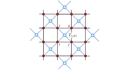
Figure 1: Tensor network representation of $q$-state clock model on square lattice.

For $q<5$, it is well known that the self-dual critical temperature readsKramers and Wannier (1941a):

$$\beta_{c}=\left\{\begin{array}[]{c}\ln\left(\sqrt{2}+1\right)/2,\text{ }q=2\\ 2\ln\left(\sqrt{3}+1\right)/3,\text{ }q=3\\ \ln\left(\sqrt{2}+1\right),\text{ }q=4\end{array}\right.$$ (4)

We will first benchmark with these exact results to examine the accuracy of our algorithm. Since the $q=2$ case has already been studied before, here we will begin with the $q=3$ and $q=4$ cases. To find the critical point, we first calculate the gauge invariant quantity $\chi$ introduced in Ref. Gu and Wen (2009):

$$\chi=\frac{\left(\underset{ij}{\sum}T_{ijij}\right)^{2}}{\underset{ijkl}{\sum}T_{ijkl}T_{klij}},$$ (5)

where we use the 2 by 2 block to represent the fixed point tensor $T$(composed by $T_{A}$ and $T_{B}$ on sublattices A and B, respectively) when calculating the gauge invariant quantity $\chi$, as shown in Fig. 2 and Fig. 3.

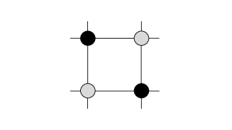
Figure 2: We use the 2 by 2 block to represent the fixed point tensor $T$ when calculating $\chi$, where we group the index $(i_{1},i_{2})$ into a single index $i$ for tensor $T$

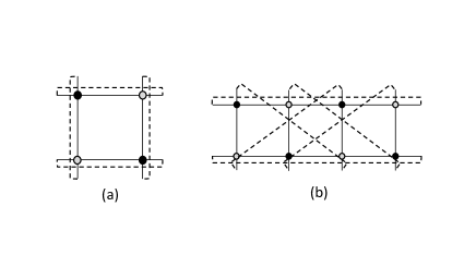
Figure 3: Gauge invariant quantity $\chi$ formed by $T$, where the numerator is represented by the square of part (a), and the denominator is given by part (b)

As seen in Fig. 4, we see that there is a sudden jump from ordered phase to disordered phase. This is because the tensors for ordered and disordered phase would flow to different fixed points. To understand better for the gauge invariant quantity $\chi$, we introduce matrix $M^{h}$ and $M^{v}$:

$$M_{ij}^{h} = \underset{k}{\sum}T_{ikjk}^{\text{fixed-point}}$$

$$M_{ij}^{v} = \underset{k}{\sum}T_{kikj}^{\text{fixed-point}}.$$ (6)

We see that for ordered phase, the eigenvalue $\lambda$ of $M^{h}$ and $M^{v}$ is:

$$\left\{\begin{array}[]{c}\lambda_{1},\lambda_{2},...\lambda_{q}=1/q\\ \text{others}=0\end{array}\right..$$ (7)

And in disordered phase, we have $\lambda_{1}=1$, and all the others approach 0, which shows clearly the symmetry breaking nature of the phase transition. Here, we have already normalized the fixed point tensor as:

$$\underset{jk}{\sum}T_{jkjk}^{\text{fixed-point}}=1.$$ (8)

Next, we compute the central charge and scaling dimensions for $q=3$ model(here we keep $D_{cut}=36$ in our loop-TNR algorithm). We find that the central charge $c=0.80005$, which is intrinsically close to the value predicted by the CFT with $c=4/5$. We see that both central charge and scaling dimensions are very stable up to 20 renormalization steps, which corresponds to a total system size $2^{23}$.

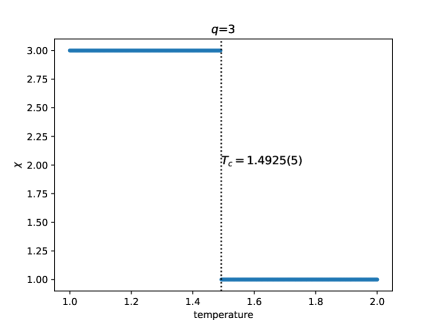
Figure 4: The invariant quantity $\chi$ as a function of temperature. We find that the critical temperature $T_{c}$ for $q=3$ model is around 1.4925(5), which is intrinsically close to the prediction of the self-dual analysis. Here we keep $D_{cut}=36$ in the loop-TNR algorithm and system size up to $2^{23}$.

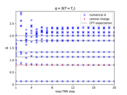
Figure 5: The scaling dimensions at the critical point of $q=3$ model with $D_{cut}$=36. We see that the conformal data rapidly converges to CFT predictions during the renormalization process.

Similarly, we can compute the gauge invariant quantity $\chi$, central charge and scaling dimensions for the $q=4$ model(again, we keep $D_{cut}=36$ in our loop-TNR algorithm), as shown in Fig. 6 and Fig. 7. We find that $c=1.00021$, which is also consistent with previous theoretical predictions with $c=1$. In fact, the critical point of $q=4$ model can be just regarded as two copies of the Ising CFT. Again, we see that both central charge and scaling dimensions are very stable up to 20 renormalization steps

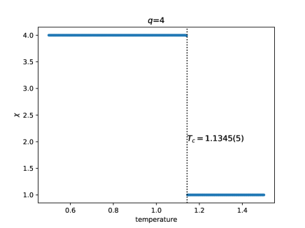
Figure 6: The invariant quantity $\chi$ as a function of temperature. We find that the critical temperature $T_{c}$ for $q=4$ model is around 1.1345(5), which is intrinsically close to the prediction of the self-dual analysisKramers and Wannier (1941a). Here we also keep $D_{cut}=36$ in the loop-TNR algorithm and system size up to $2^{23}$.

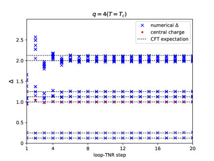
Figure 7: The scaling dimensions at the critical point of $q=4$ model with $D_{cut}$=36.

III $q=5$ and $q=6$ models

For $q\geq 5$, it is conjectured that the $q$-state clock model is described by $Z_{q}$ -deformed sine-Gordon theoryWiegmann (1978); Matsuo and Nomura (2006)

$$S = \frac{1}{2\pi K}\int d^{2}\mathbf{r}\left(\mathbf{\nabla}\phi\right)^{2}+\frac{g_{1}}{2\pi\alpha^{2}}\int d^{2}\mathbf{r}\cos\left(\sqrt{2}\phi\right)$$ (9)

$$+\frac{g_{2}}{2\pi\alpha^{2}}\int d^{2}\mathbf{r}\cos\left(q\sqrt{2}\Theta\right),$$

where $\phi,\Theta$ are compactified as $\phi\equiv\phi+\sqrt{2}\pi$, $\Theta\equiv\Theta+\sqrt{2}\pi,$ and they satisfy the dual relation $\partial_{x}\phi=-K\partial_{y}\Theta,$ $\partial_{y}\phi=K\partial_{x}\Theta.$ The coupling constants $K,g_{1},g_{2}$ are temperature-dependent, and $\alpha$ is a UV cutoff.

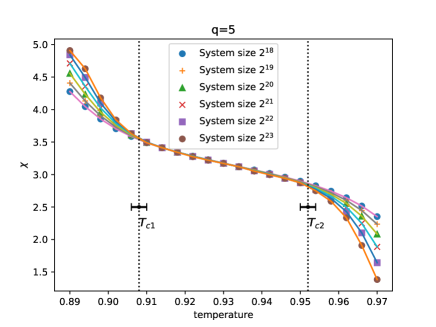
Figure 8: Invariant quantity of $q=5$ model. In ordered phase, the gauge invariant quantity $\chi$ should flow to the fixed point $\chi=5$, while in disordered phase, $\chi$ should flow to $\chi=1$. In the middle phase, the value of $\chi$ varies with temperature. We can read out that $T_{c1}=0.908(2)$, and $T_{c2}=0.952(2)$.

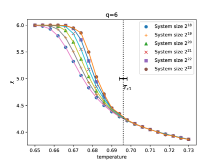
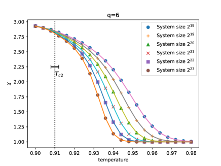
Figure 9: Invariant quantity of $q=6$ model around $T_{c1}$ and $T_{c2}$. We can read that $T_{c1}=0.696(2)$, and $T_{c2}=0.912(2)$, with the same analysis with $q=5$ model.

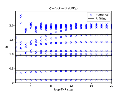
Figure 10: An example of scaling dimensions in the critical phase for $q=5$ model.

With decreasing temperature, the above effective theory will describe two phase transitions, which can be understood from the renormalization group flow of the second and third terms. The high-temperature critical point is described by the well known BKT transition while the low-temperature transition is described by the usual symmetry breaking transition. As the coupling $g_{1}$ and $g_{2}$ become irrelevant between the two critical point $T_{c1}<T<T_{c2}$, the effective theory reduces to the compactified boson theory in the middle phase, with compatification radius $R=\sqrt{2K}$. In addition, if $g_{1}=g_{2}$, Eq. (9) is self-dual. From the scaling dimension analysis, the compactification radius can be computed exactly for both phase transition points as well as for the self-dual pointLi et al. (2020). We have:

$$R_{c2} = 2\sqrt{2},\text{ BKT transition point}$$

$$R_{self-dual} = \sqrt{2q},\text{ self-dual point}$$

$$R_{c1} = q/\sqrt{2},\text{ symmetry-breaking point}$$

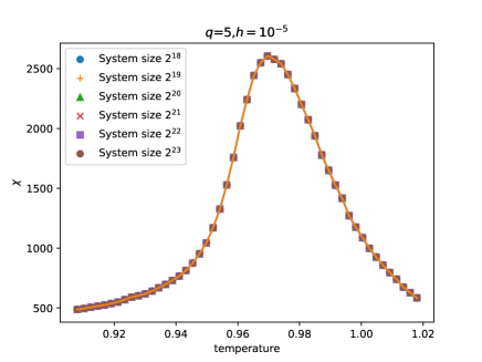
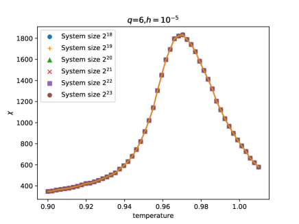
Figure 11: Susceptibility of $q=5$ and $q=6$ models with external field $h=10^{-5}$.

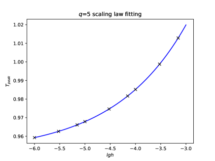
Figure 12: Susceptibility peak temperature versus external field for $q=5$ model, from which we find that $T_{c}=0.9507(5)$, $a=0.5605$, $b=0.3028$.

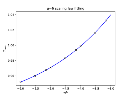
Figure 13: Susceptibility peak temperature versus external field for $q=6$ model, from which we find that $T_{c}=0.9111(5)$, $a=0.4057$, $b=0.1662$.

	$T_{c1}$	$T_{c2}$
$q=5$
Ref.Tobochnik (1982)	0.8	1.1
Ref.Borisenko et al. (2011)	0.905(1)	0.951(1)
Ref.Kumano et al. (2013)	0.908	0.944
Ref.Chatelain (2014)	0.914(12)	0.945(17)
Ref.Chatterjee et al. (2018)	0.897(1)	-
Ref.Chen et al. (2018)	0.9029(1)	0.9520(1)
Ref.Surungan et al. (2019)	0.911(5)	0.940(5)
Ref.Hong and Kim (2020)	0.908	0.945
Ref.Li et al. (2020)	0.9059(2)	0.9521(2)
our result	0.908(2)	0.9507(5)
$q=6$
Ref.Tobochnik (1982)	0.6	1.3
Ref.Challa and Landau (1986)	68(2)	0.92(1)
Ref.Yamagata and Ono (1991)	0.68	0.90
Ref.Tomita and Okabe (2002)	0.7014(11)	0.9008(6)
Ref.Hwang (2009)	0.632(2)	0.997(2)
Ref.Brito et al. (2010)	0.68(1)	0.90(1)
Ref.Baek et al. (2013)	-	0.9020(5)
Ref.Kumano et al. (2013)	0.700(4)	0.904(5)
Ref.Krcmar et al. (2016)	0.70	0.88
Ref.Chen et al. (2017)	0.6658(5)	0.8804(2)
Ref.Chatterjee et al. (2018)	0.681(1)	-
Ref.Surungan et al. (2019)	0.701(5)	0.898(5)
Ref.Hong and Kim (2020)	0.693	0.904
Ref.Li et al. (2020)	0.6901(4)	0.9127(5)
our results	0.696(2)	0.9111(5)

Table 1: A comparison of $T_{c1}$ and $T_{c2}$ with previous results by using other methods.

Similar to the $q<5$ model, two transition points of $q=5$ model can be read out from the gauge invariant quantity $\chi$. In Fig. 8, we plot $\chi$ as a function of temperature near the critical point. Very different from the $q<5$ model, there is no sharp change in $\chi$ near the two phase transition points. Similar to the $q<5$ model, in ordered phase, the tensor would flow to the fixed point with $\chi=5$, while in disordered phase, the fixed point tensor gives rise to $\chi=1$. However, in the middle phase, The structure of fixed point tensor is very complicated and we will discuss the details later. An interesting feature is that the gauge invariant quantity $\chi$ becomes size independent in the middle critical phase and this help us pin down the critical temperature for both high-temperature and low-temperature phase transitions. As seen from Fig. 8, we can read out that the low temperature symmetry breaking transition point $T_{c1}$ is around 0.908(2) while the high-temperature BKT phase transition point is around 0.952(2). Similar analysis can be applied to $q=6$ model as well, and we can read out from Fig. 9 that the low-temperature critical point $T_{c1}$ is around 0.696(2), and high-temperature phase transition point $T_{c2}$ is around 0.912(2). We note that in order to increase the accuracy, here and below we will use the $Z_{q}$ symmetric loop-TNR algorithm(see Appendix B for more details) with $D_{cut}=8q$ for simulating all $q$-state clock models.

Since the middle phase is described by compactified boson model, we can further use the fixed point tensor to compute its central charge and scaling dimensions. As seen in Fig. 10, we find $c=0.99987$ for $q=5$ model with $T=0.93k_{B}/J$, which is intrinsically close to the theoretical prediction with $c=1$. It is well known that the scaling dimensions of the primary fields of the compactified boson model can be expressed as:

$$\Delta_{e,m}=\frac{m^{2}}{R^{2}}+\frac{e^{2}R^{2}}{4},$$ (10)

where $R$ is the compactified radius and $m,e$ are integers which label the primary fields. In Fig. 10, we also plot the scaling dimension for $q=5$ model with $T=0.93k_{B}/J$. We find that all the low scaling dimension can be fit quite well with $R=3.08607$.(We choose the scaling dimensions of RG steps from 15-20 to fit the compactification radius $R$). We note that the deviations for high scaling dimensions are due to the numerical error and we can further improve the accuracy by increasing $D_{cut}$ in the loop-TNR algorithm.

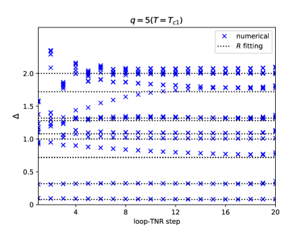
Figure 14: Scaling dimensions at the critical point $T_{c1}$ and $T_{c2}$ for $q=5$ model, from which we can fit the compactifiction radius $R$ of the compactified boson theory. We find that at $T_{c1}$, $R=3.52954$, and at $T_{c2}$, $R=2.83894$.

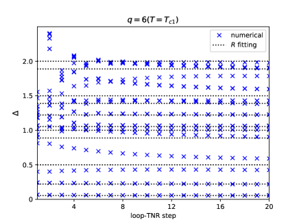
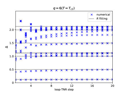
Figure 15: Scaling dimensions at the critical point $T_{c1}$ and $T_{c2}$ for $q=6$ model, from which we can fit the compactification radius $R$ of the compactified boson theory. We find that at $T_{c1}$, $R=4.23870$, and at $T_{c2}$, $R=2.82024$.

The BKT transition point $T_{c2}$ can also be determined by the susceptibility peak method with extremely high accuracy. First, by applying a very small external field, we can compute the susceptibility at different external field $h$ and temperature $T$Yu et al. (2014):

$$\chi\left(h,T\right)=\left.\frac{\partial m}{\partial h}\right|_{T}.$$ (11)

For example, in Fig. 11, we plot the susceptibility function at different system size for $q=5$ and $q=6$ models with a very small external field $h=10^{-5}$. We see that all the susceptibility functions collapse to a single curve, which implies the thermodynamic limit has already been achieved for physical quantities despite the fact that the gauge invariant quantity $\chi$ still has very strong size dependence near both critical temperatures. By plotting the peak position of $\chi$ with different external fields, we can read out $T_{c2}$ by using the following formula:

$$T_{peak}\left(h\right)=T_{c}+ah^{b}.$$ (12)

We find that for $q=5$ model, $T_{c2}=0.9507(5)$, $a=0.5605$, $b=0.3028$, and for $q=6$ model, $T_{c2}=0.9111(5)$, $a=0.4057$, $b=0.1662$. Fig. 12 and Fig. 13 show the susceptibility-peak fitting for $q=5$ and $q=6$ models, respectively. We see that the results of $T_{c2}$ is comparable with what we get from the gauge invariant quantity $\chi$.

In Table 1, we compare our results with all previous known results for $T_{c1}$ and $T_{c2}$ using other methods. We see that our method gives much more accurate critical temperatures than HOTRG based methodChen et al. (2017, 2018), and the results are comparable with recent MPS based methodLi et al. (2020) and large scale Monte-Carlo resultsBorisenko et al. (2011); Surungan et al. (2019). We note that the small disagreement in the last digit might arise from the finite size effect in other methods. Our loop-TNR method can handle system size up to $2^{23}$ with very high accuracy.

We further compute the scaling dimensions at $T_{c1}$ and $T_{c2}$ for of both $q=5$ and $q=6$ models. From the results of scaling dimension at each RG step, we can clearly observe the logarithmic flow of some higher scaling dimensions, as seen in Fig. 14 and Fig. 15. This implies the existence of marginal irrelevant termsJanke (1997) for these transition points, and it explains why these transition points are very hard to be determined accurately in previous studies. From the scaling dimensions, we can fit the compactification radius $R$ by using Eq. (10). In Table 2, we list the compactification radius $R$ at both transition points and we find a perfect agreement with the field theory predictions. We stress that comparing with the very recent studies by using MPS based methodLi et al. (2020), our results give rise to much more accurate compactification radius $R$ at these phase transition points.

Finally, we investigate the scaling dimensions and compactification radius $R$ for the so-called self-dual point. The element tensor for dual model in Fig. 16, which is obtained by Kramers-Wannier transformationKramers and Wannier (1941a, b); Zamolodchikov and Monastyrski (1979), could be expressed as:

$$\widetilde{T}_{abcd} = \exp\frac{\beta}{2}\left(\cos\theta_{a}+\cos\theta_{b}+\cos\theta_{c}+\cos\theta_{d}\right)$$ (13)

$$\times \delta_{\rm{mod}(a+b+c+d,q),0}$$

To determine the self-dual temperature, we compute the magnetization at different temperatures for both $q$-state model and its dual model. As seen in Fig. 17, the crossing point corresponds to the dual temperature with $g_{1}=g_{2}$. Again, we can use the loop-TNR algorithm to compute the scaling dimensions(see in Fig. 18) and from the scaling dimension data, we can further fit the compactification $R$. In Table 2, we compare our results with the theoretical predictions. Again, we find a perfect agreement for both $q=5$ and $q=6$ models.

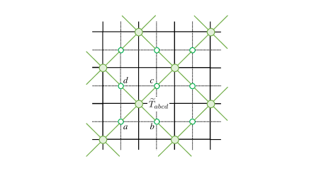
Figure 16: Tensor network representation of dual model, where the original lattice is shown by solid line and the dual lattice is shown by dash line.

$q$	$T_{c1}$		$T_{dual}$		$T_{c2}$
	theory	numerical	theory	numerical	theory	numerical
5	$\sqrt{25/2}$	3.52954	$\sqrt{10}$	3.17354	$2\sqrt{2}$	2.83894
6	$\sqrt{18}$	4.23870	$\sqrt{12}$	3.46002	$2\sqrt{2}$	2.82024

Table 2: Compactification radius $R$ on both critical points as well as self-dual point of $q$-state clock model with $q=5$ and $q=6$.

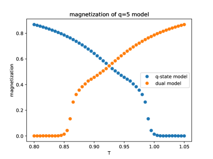
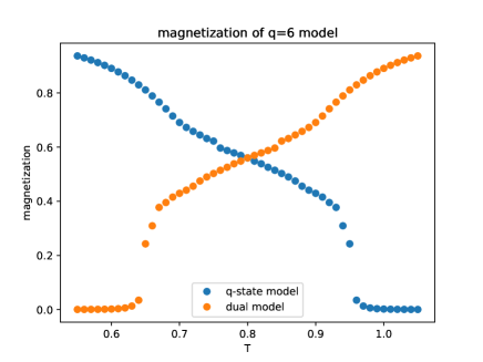
Figure 17: Magnetization of $q$-state clock model with $q=5,6$ and their corresponding dual model.

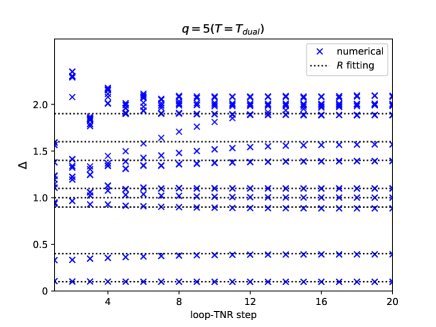
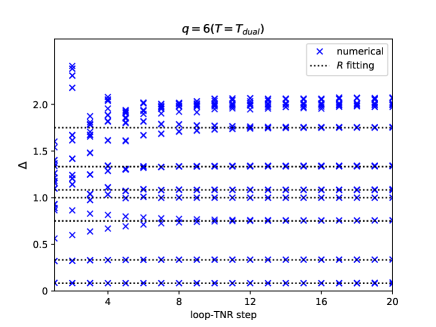
Figure 18: Scaling dimension on self-dual point for $q=5$ and $q=6$ models, from which we can fit the compactification radius $R$ of the compactified boson theory. We find that $R=3.17354$ for $q=5$ and $R=3.46002$ for $q=6$ model.

IV $q>6$ models and fixed point tensor for BKT transition

IV.1 Critical temperature and compactification radius

By using the same methods for $q=5$ and $q=6$ models, we also studies the phase diagram for $q>6$ models. By computing both the gauge invariant quantity $\chi$ and fitting the susceptibility peak position under different external field, we can determine both $T_{c1}$ and $T_{c2}$ accurately. In Table 3, we compare our results for $q=7,8,9$ models with previous studies using other methods. Remarkably, for models with big enough $q$, i.e., $q>6$, $T_{c2}$ becomes very close to the BKT transition value in classical XY model with $T_{c}=0.8929$.

Similar to $q=5$ and $q=6$ models, we can also use loop-TNR method to compute the scaling dimensions and fit the corresponding compactification radius $R$, see Appendix A for more details. We find that the radius $R$ at $T_{c2}$ also saturates to a fixed value 2.81987 for big enough $q$, which is intrinsically close to the theoretical prediction $R=2\sqrt{2}$. We can also use the same method for $q=5$ and $q=6$ models to determine the self-dual point and fit the corresponding compactification radius $R$. In Table 4, we also list the compactification radius $R$ for $T_{c1}$ and self-dual point $T_{dual}$. Again, we find a perfect agreement with theoretical predictions.

	$T_{c1}$	$T_{c2}$
$q=7$
Ref.Borisenko et al. (2012)	0.533	0.900
Ref.Chatterjee et al. (2018)	0.531(6)	-
Ref.Li et al. (2020)	0.5305(3)	0.9071(5)
our results	0.536(2)	0.9065(5)
$q=8$
Ref.Tomita and Okabe (2002)	0.4259(4)	0.8936(7)
Ref.Baek et al. (2009)	0.417(3)	0.894(1)
Ref.Chatterjee et al. (2018)	0.418(1)	-
Ref.Li et al. (2020)	0.4172(3)	0.9060(5)
our results	0.4215(15)	0.9051(5)
$q=9$
Ref.Chatterjee et al. (2018)	0.334(1)	-
our results	0.342(2)	0.9051(5)

Table 3: A comparison of $T_{c1}$ and $T_{c2}$ with previous results by using other methods.

$q$	$T_{c1}$		$T_{dual}$		$T_{c2}$
	theory	numerical	theory	numerical	theory	numerical
7	$\sqrt{49/2}$	4.94072	$\sqrt{14}$	3.75035	$2\sqrt{2}$	2.83153
8	$\sqrt{32}$	5.67377	$\sqrt{16}$	4.00726	$2\sqrt{2}$	2.81987
9	$\sqrt{81/2}$	6.36759	$\sqrt{18}$	4.23573	$2\sqrt{2}$	2.81987

Table 4: Compactification radius $R$ on critical points and self-dual point for $q=7,8,9$ models.

IV.2 Fixed point tensor for BKT transition

Since the $T_{c2}$ for $q>6$ models is already very close to the BKT transition in classical XY model, and the compactification radius $R$ is also approaching the expected value for BKT transition, it is natural to ask whether the corresponding fixed point tensors in these models also converge to the same one(up to numerical errors) which contains the complete information for BKT transitions. Below we will study the structure of fixed point tensor for $q>6$ models at BKT transition and try to read out the OPE coefficient directly for the corresponding compactified boson CFT.

IV.2.1 The gauge choice of the fixed point tensor

It is well known that there exists a gauge degree of freedom for the fixed point tensor in any TNR scheme and it is actually the major difficulty for us to understand the full structure of fixed point tensors for critical systems.

We will begin with some general discussion for the nature of such a gauge degree of freedom and explain why it can be fixed by introducing enough symmetry conditions. Apparently, if we apply some invertible matrices on every legs of a tensor, the transformed tensor actually forms the same tensor network as before:

$$T_{ijkl}^{\prime}=\underset{i^{\prime}j^{\prime}k^{\prime}l^{\prime}}{\sum}T_{i^{\prime}j^{\prime}k^{\prime}l^{\prime}}U_{i^{\prime}i}V_{j^{\prime}j}\left[U^{-1}\right]_{kk^{\prime}}\left[V^{-1}\right]_{ll^{\prime}}$$ (14)

This gives rise to great difficulty to analyze the properties of the tensor components of the fixed point tensor, since they could be randomly affected by the gauge choice in numerical calculations. To get a proper gauge fixing, we have the following considerations:

$\bullet$ The fixed point tensor(defined on the 2 by 2 plaquette composed by $T_{A}$ and $T_{B}$ tensors, as shown in Fig. 2) should preserve the $C_{4}$ lattice symmetry during the loop-TNR process(see Appendix B for more details). Preserving $C_{4}$ symmetry will reduce the gauge freedom of the fixed point tensor. The gauge transformation in Eq. (14) can be simplified as:

$$T_{ijkl}^{\prime}=\underset{i^{\prime}j^{\prime}k^{\prime}l^{\prime}}{\sum}T_{i^{\prime}j^{\prime}k^{\prime}l^{\prime}}O_{i^{\prime}i}O_{j^{\prime}j}O_{k^{\prime}k}O_{l^{\prime}l}$$ (15)

where $O$ is an orthogonal matrix.(We assume all the tensors are real.)

$\bullet$ Since the $q$-state clock model has a $Z_{q}$ internal symmetry, we should also keep such an internal symmetry during the whole loop-TNR process(see Appendix B for more details). By keeping the $Z_{q}$ symmetry, we can further reduce the gauge degrees of freedom. In fact this is a crucial step to obtain the right fusion rule for fixed point tensor. It is well known that the fusion rule of compactifiled boson theory has a $U(1)$ symmetry which can be realized explicitly on $XY$ model. However, if we only focus on the leading components of primary fields and descendant fields, $Z_{q}$ symmetry is a very good approximation for $U(1)$.

$\bullet$ If we want the indices of the fixed point tensor to represent the primary fields and their descendants for the corresponding compactified boson theory, we need to choose a proper basis. The eigenstate of the transfer matrix is a good choice. As shown in Fig. 19 (d), we construct a rank-3 tensor with the building block tensor $M_{ijkl}$ in $C_{4}$-loop-TNR algorithm(see Appendix B for more details). This is because in usual CFT, the 3-point correlation function is more fundamental and has a much simpler form than the 4-point correlation function. In fact, the basic renormalzation step in loop-TNR is similar to the crossing symmetry for 4-point correlation function. Thus, we conjecture that the rank-3 tensor constructed here could be regarded as a 3-point correlation function(at least for primary fields). As illustrated in Fig. 20, we construct the $2\times 2$ transfer matrix as shown in Fig 20 (a), and apply the eigenvalue decomposition:

$$M_{(i_{1}i_{2})\left(j_{1}j_{2}\right)}=\underset{k}{\sum}U_{(i_{1}i_{2})k}\lambda_{k}\left[U^{-1}\right]_{k(i_{1}i_{2})}.$$ (16)

We use eigenvectors $U_{(i_{1}i_{2})i}$ as the basis for the fixed point tensor, as shown in Fig. 20 (b). As a result, the fixed point tensor is projected onto the basis representing primary fields and their descendants.

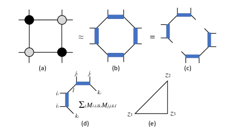
Figure 19: From loop-TNR algorithm, a square fixed point tensor (a) could be approximately represented by MPS on the octagon lattice (b). Then, we decompose octagon MPS from (b) to (c). The rank-3 tensor in (d) is the fixed point tensor we will study here. (e) The geometry of the corresponding 3-point correlation functions.

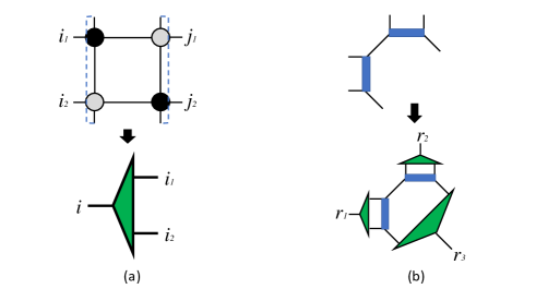
Figure 20: (a) We choose the eigenstates of the transfer matrix in as our basis. (b) We then project the rank-3 fixed point tensors on to these basis.

IV.2.2 Operator product expansion(OPE) coefficient from the fixed point tensor

In Table 5, we list the leading non-zero components of the fixed point tensors of different $q$-state clock models at BKT critical point. Here we normalize the largest component $T_{III}=1$. We use $I$, $\alpha$, $\beta$, $\gamma$, $\delta$, $\lambda$ and $\eta$ to represent the leading primary fields $(0,0)$, $(1,0)$, $(-1,0)$, $(2,0)$, $(-2,0)$, $(3,0)$ and $(-3,0)$.

$T^{q=7}_{r_{1}r_{2}r_{3}}$	$T^{q=8}_{r_{1}r_{2}r_{3}}$	$T^{q=9}_{r_{1}r_{2}r_{3}}$	$T^{q=10}_{r_{1}r_{2}r_{3}}$	$r_{1}$	$r_{2}$	$r_{3}$
1.00000	1.00000	1.00000	1.00000	$I$	$I$	$I$
0.81215	0.81594	0.81555	0.81725	$I$	$\alpha$	$\beta$
0.81215	0.81594	0.81555	0.81725	$I$	$\beta$	$\alpha$
0.44178	0.44747	0.45242	0.45253	$I$	$\gamma$	$\delta$
0.44178	0.44747	0.45242	0.45253	$I$	$\delta$	$\gamma$
0.81215	0.81594	0.81555	0.81725	$\alpha$	$I$	$\beta$
0.59058	0.59609	0.59756	0.59821	$\alpha$	$\alpha$	$\delta$
0.74242	0.74698	0.74671	0.74901	$\alpha$	$\beta$	$I$
0.45419	0.46021	0.49495	0.46479	$\alpha$	$\delta$	$\alpha$
0.81215	0.81594	0.81555	0.81725	$\beta$	$I$	$\alpha$
0.74242	0.74698	0.74671	0.74901	$\beta$	$\alpha$	$I$
0.59058	0.59609	0.59756	0.59821	$\beta$	$\beta$	$\gamma$
0.45419	0.46021	0.46369	0.46479	$\beta$	$\gamma$	$\beta$
0.44178	0.44747	0.45242	0.45253	$\gamma$	$I$	$\delta$
0.45419	0.46021	0.46369	0.46479	$\gamma$	$\beta$	$\beta$
0.30919	0.31491	0.32114	0.32120	$\gamma$	$\delta$	$I$
0.44178	0.44747	0.45242	0.45253	$\delta$	$I$	$\gamma$
0.45419	0.46021	0.46369	0.46479	$\delta$	$\alpha$	$\alpha$
0.30919	0.31491	0.32114	0.32120	$\delta$	$\gamma$	$I$

Table 5: A comparison of non-zero leading components of the fixed point tensor of q-state clock models with $q=7,8,9,10$ at BKT critical point.

It is well known that the fusion rule of the primary fields in compactified boson theory satisfies:

$$\left[\phi_{e_{1},m_{1}}\right]\times\left[\phi_{e_{2},m_{2}}\right]=\left[\phi_{e_{1}+e_{2},m_{1}+m_{2}}\right],$$ (17)

where $\left[\phi_{e,m}\right]$ is a conformal family generated by primary field $\phi_{e,m}$ with conformal dimension $\left(\left(e/R+mR/2\right)^{2}/2,\left(e/R-mR/2\right)^{2}/2\right)$. In particular, the primary field with $m=0$ is just the vertex operator and it can be written as:

$$\phi_{e,0}\left(z,\overline{z}\right)=e^{ie\varphi\left(z,\overline{z}\right)/R},$$ (18)

with $\varphi\left(z,\overline{z}\right)$ the free boson field. The 3-point function has a pretty simple form:

$$\langle\phi_{e_{1},0}\left(z_{1},\overline{z}_{1}\right)\phi_{e_{2},0}\left(z_{2},\overline{z}_{2}\right)\phi_{e_{3},0}\left(z_{3},\overline{z}_{3}\right)\rangle$$ (19)

$$= \frac{C_{123}}{\left|z_{12}\right|^{\Delta_{1}+\Delta_{2}-\Delta_{3}}\left|z_{23}\right|^{\Delta_{2}+\Delta_{3}-\Delta_{1}}\left|z_{31}\right|^{\Delta_{3}+\Delta_{1}-\Delta_{2}}},$$

where $C_{123}$ is the OPE coefficient, which equals 1 for $e_{1}+e_{2}+e_{3}\neq 0$ and vanishes for $e_{1}+e_{2}+e_{3}=0$. $\left|z_{12}\right|\equiv\left|z_{1}-z_{2}\right|$, and the scaling dimension $\Delta_{i}=\frac{e_{i}^{2}}{R^{2}}$. We note that in general only leading primary fields in our numerical fixed point tensor can satisfy the fusion rule since we use the $Z_{q}$ symmetry to approximate the $U(1)$ symmetry in the gauge fixing procedure, and with increasing $q$, more and more primary fields with correct fusion rules can be resolved numerically. (Although we believe that the emergent $U(1)$ must be present for all finite $q$ with $q>4$, it is in general very hard to find the proper gauge choice for small $q$, especially for $q=5$ and $q=6$.)

Next, we can try to fit our numerical fixed point tensor by using the 3-point correlation function Eq. (19). Let $z_{13}=\lambda_{1}x$, $z_{23}=\lambda_{2}x$, $z_{12}=\lambda_{3}x$. We can rewrite the right hand side of Eq. (19) as:

$$\frac{C_{123}}{\left(\lambda_{1}x\right)^{\Delta_{1}+\Delta_{3}-\Delta_{2}}\left(\lambda_{2}x\right)^{\Delta_{2}+\Delta_{3}-\Delta_{1}}\left(\lambda_{3}x\right)^{\Delta_{1}+\Delta_{2}-\Delta_{3}}}$$ (20)

$$= C_{123}\left(\frac{\lambda_{2}}{\lambda_{1}\lambda_{3}x}\right)^{\Delta_{1}}\left(\frac{\lambda_{1}}{\lambda_{2}\lambda_{3}x}\right)^{\Delta_{2}}\left(\frac{\lambda_{3}}{\lambda_{1}\lambda_{2}x}\right)^{\Delta_{3}}$$

$$\equiv C_{123}l_{1}^{\Delta_{1}}l_{2}^{\Delta_{2}}l_{3}^{\Delta_{3}},$$

with $l_{1}=\frac{\lambda_{2}}{\lambda_{1}\lambda_{3}x}$, $l_{2}=\frac{\lambda_{1}}{\lambda_{2}\lambda_{3}x}$ and $l_{3}=\frac{\lambda_{3}}{\lambda_{1}\lambda_{2}x}$, respectively. From the geometry of the square lattice, we conjecture that our rank-3 fixed point tensor can be regarded as 3-point correlation(at least for primary fields) function on the vertex of an isosceles right triangle on the complex plane, as seen in Fig. 19 (e). Thus we can choose $\lambda_{1}=\lambda_{2}=\lambda_{3}/\sqrt{2}=1$ and Eq. (20) can be simplified as:

$$C_{123}l_{1}^{\Delta_{1}}l_{2}^{\Delta_{2}}l_{3}^{\Delta_{3}}\equiv C_{123}l^{\Delta_{1}}l^{\Delta_{2}}\left(2l\right)^{\Delta_{3}}.$$ (21)

where $l=\frac{1}{\sqrt{2}x}$ is a fundamental inverse length scale. For $q=10$ model at the temperature $T_{c2}$, the non-zero leading components of fixed point tensor are given by Table 6. If we fit our data with Eq. (21), we find:

$$\Delta_{\left(\pm 1,0\right)} = 0.12684$$

$$\Delta_{\left(\pm 2,0\right)} = 0.50869$$

$$\Delta_{\left(\pm 3,0\right)} = 1.17789,$$ (22)

which match well with the results from our previous transfer matrix calculation, with $\Delta_{\left(\pm 1,0\right)}=0.12539$, $\Delta_{\left(\pm 2,0\right)}=0.50158$ and $\Delta_{\left(\pm 3,0\right)}=1.12851$(the corresponding compactification radius $R=2.82402$). The fundamental length scale can also be fitted as $x=2.23035$, and the corresponding OPE coefficients are listed in Table 7. The relative error of our fitting is estimated as:

$$\sqrt{\frac{\underset{N}{\sum}\left[\left|\left|T_{r_{1}r_{2}r_{3}}\right|-C_{123}l^{\Delta_{1}}l^{\Delta_{2}}\left(2l\right)^{\Delta_{3}}\right|/\left|T_{r_{1}r_{2}r_{3}}\right|\right]^{2}}{N}},$$ (23)

where $N$ is the total number of components in our consideration. We find the fitting error is around $4.0\times 10^{-3}$. Thus, we conclude that the fixed point tensor can be well described by the 3-point function(at least for primary fields) and the OPE coeeficient can be read out directly.

$T_{r_{1}r_{2}r_{3}}$	$r_{1}$	$r_{2}$	$r_{3}$	$T_{r_{1}r_{2}r_{3}}$	$r_{1}$	$r_{2}$	$r_{3}$
1.00000	$I$	$I$	$I$	0.45253	$\gamma$	$I$	$\delta$
0.81725	$I$	$\alpha$	$\beta$	0.30155	$\gamma$	$\alpha$	$\eta$
0.81725	$I$	$\beta$	$\alpha$	0.46479	$\gamma$	$\beta$	$\beta$
0.45253	$I$	$\gamma$	$\delta$	0.32120	$\gamma$	$\delta$	$I$
0.45253	$I$	$\delta$	$\gamma$	0.15522	$\gamma$	$\eta$	$\alpha$
0.17675	$I$	$\lambda$	$\eta$	0.45253	$\delta$	$I$	$\gamma$
0.17675	$I$	$\eta$	$\lambda$	0.46479	$\delta$	$\alpha$	$\alpha$
0.81725	$\alpha$	$I$	$\beta$	0.30155	$\delta$	$\beta$	$\lambda$
0.59820	$\alpha$	$\alpha$	$\delta$	0.32120	$\delta$	$\gamma$	$I$
0.74901	$\alpha$	$\beta$	$I$	0.15522	$\delta$	$\lambda$	$\beta$
0.30155	$\alpha$	$\gamma$	$\eta$	0.17675	$\lambda$	$I$	$\eta$
0.46479	$\alpha$	$\delta$	$\alpha$	0.20004	$\lambda$	$\beta$	$\delta$
0.20004	$\alpha$	$\eta$	$\gamma$	0.15522	$\lambda$	$\delta$	$\beta$
0.81725	$\beta$	$I$	$\alpha$	0.08449	$\lambda$	$\eta$	$I$
0.74901	$\beta$	$\alpha$	$I$	0.17675	$\eta$	$I$	$\lambda$
0.59820	$\beta$	$\beta$	$\gamma$	0.20004	$\eta$	$\alpha$	$\gamma$
0.46479	$\beta$	$\gamma$	$\beta$	0.15522	$\eta$	$\gamma$	$\alpha$
0.30155	$\beta$	$\delta$	$\lambda$	0.08449	$\eta$	$\lambda$	$I$
0.20004	$\beta$	$\lambda$	$\delta$

Table 6: Leading non zero components of the fixed point tensor of $q=10$ model at BKT critical point $T_{c2}$.

$C_{r_{1}r_{2}r_{3}}$	$r_{1}$	$r_{2}$	$r_{3}$	$C_{r_{1}r_{2}r_{3}}$	$r_{1}$	$r_{2}$	$r_{3}$
1.00000	$I$	$I$	$I$	1.00000	$\gamma$	$I$	$\delta$
1.00000	$I$	$\alpha$	$\beta$	1.01105	$\gamma$	$\alpha$	$\eta$
1.00000	$I$	$\beta$	$\alpha$	1.00350	$\gamma$	$\beta$	$\beta$
1.00000	$I$	$\gamma$	$\delta$	1.00000	$\gamma$	$\delta$	$I$
1.00000	$I$	$\delta$	$\gamma$	0.99779	$\gamma$	$\eta$	$\alpha$
1.00000	$I$	$\lambda$	$\eta$	1.00000	$\delta$	$I$	$\gamma$
1.00000	$I$	$\eta$	$\lambda$	1.00350	$\delta$	$\alpha$	$\alpha$
1.00000	$\alpha$	$I$	$\beta$	1.01105	$\delta$	$\beta$	$\lambda$
1.00023	$\alpha$	$\alpha$	$\delta$	1.00000	$\delta$	$\gamma$	$I$
1.00000	$\alpha$	$\beta$	$I$	0.99779	$\delta$	$\lambda$	$\beta$
1.01105	$\alpha$	$\gamma$	$\eta$	1.00000	$\lambda$	$I$	$\eta$
1.00350	$\alpha$	$\delta$	$\alpha$	0.99590	$\lambda$	$\beta$	$\delta$
1.01105	$\alpha$	$\eta$	$\gamma$	0.99779	$\lambda$	$\delta$	$\beta$
1.00000	$\beta$	$I$	$\alpha$	1.00000	$\lambda$	$\eta$	$I$
1.00000	$\beta$	$\alpha$	$I$	1.00000	$\eta$	$I$	$\lambda$
1.00023	$\beta$	$\beta$	$\gamma$	0.99590	$\eta$	$\alpha$	$\gamma$
1.00350	$\beta$	$\gamma$	$\beta$	0.99779	$\eta$	$\gamma$	$\alpha$
1.01105	$\beta$	$\delta$	$\lambda$	1.00000	$\eta$	$\lambda$	$I$
0.99590	$\beta$	$\lambda$	$\delta$

Table 7: Fitting OPE coefficients in Eq. (19) of $q=10$ model at temperature $T=T_{c2}$, we see that they approach the expected value 1.

IV.3 Fixed point tensor for general cases

In fact, the above structure of fixed point tensor holds for the whole critical phase between $T_{c1}$ and $T_{c2}$. In the following, we further study the fixed point tensor for the $q=10$ case at different temperatures. Table 8 shows that all the OPE coefficients are very close to 1, as expected from the compactified boson theory. Table 9 shows the comparison between the scaling dimensions read from the fixed point tensor and from the direct calculation of transfer matrix. We see that they also match very well.

$C^{t=0.70}_{r_{1}r_{2}r_{3}}$	$C^{t=0.76}_{r_{1}r_{2}r_{3}}$	$C^{t=0.80}_{r_{1}r_{2}r_{3}}$	$r_{1}$	$r_{2}$	$r_{3}$
1.00000	1.00000	1.00000	$I$	$I$	$I$
1.00000	1.00000	1.00000	$I$	$\alpha$	$\beta$
1.00000	1.00000	1.00000	$I$	$\beta$	$\alpha$
1.00000	1.00000	1.00000	$I$	$\gamma$	$\delta$
1.00000	1.00000	1.00000	$I$	$\delta$	$\gamma$
1.00000	1.00000	1.00000	$\alpha$	$I$	$\beta$
0.99967	0.99961	0.99955	$\alpha$	$\alpha$	$\delta$
1.00000	1.00000	1.00000	$\alpha$	$\beta$	$I$
1.00016	1.00015	1.00010	$\alpha$	$\delta$	$\alpha$
1.00000	1.00000	1.00000	$\beta$	$I$	$\alpha$
1.00000	1.00000	1.00000	$\beta$	$\alpha$	$I$
0.99967	0.99961	0.99955	$\beta$	$\beta$	$\gamma$
1.00016	1.00015	1.00010	$\beta$	$\gamma$	$\beta$
1.00000	1.00000	1.00000	$\gamma$	$I$	$\delta$
1.00016	1.00015	1.00010	$\gamma$	$\beta$	$\beta$
1.00000	1.00000	1.00000	$\gamma$	$\delta$	$I$
1.00000	1.00000	1.00000	$\delta$	$I$	$\gamma$
1.00016	1.00015	1.00010	$\delta$	$\alpha$	$\alpha$
1.00000	1.00000	1.00000	$\delta$	$\gamma$	$I$

Table 8: OPE coefficient in Eq. (19) fitting from the data of model $q=10$ on different tempreature

Temperature	$\Delta_{1}$	$\Delta_{2}$	$\Delta_{3}$	Fitting radius $R$
From fixed point tensor
0.70	0.06941	0.27824	0.62659	3.79267
0.72	0.07228	0.28971	0.65169	3.72312
0.74	0.07532	0.30182	0.67813	3.64573
0.76	0.07851	0.31456	0.70589	3.57106
0.78	0.08191	0.32813	0.73536	3.49684
0.80	0.08566	0.34298	0.76683	3.41513
From transfer matrix
0.70	0.06940	0.27795	0.62510	3.79498
0.72	0.07217	0.28845	0.65024	3.72290
0.74	0.07508	0.30057	0.67854	3.64905
0.76	0.07830	0.31386	0.70314	3.57325
0.78	0.08178	0.32827	0.73366	3.49727
0.80	0.08571	0.34675	0.76734	3.41494

Table 9: Scaling dimension of the first 3 levels reads by fitting fixed point tensor with 3-point function of CFT and from the calculation of transfer matrix.

Therefore, we find very strong evidence that the fixed point tensor can be described by three-point correlation function for primary fields. Such a structure also explains why loop-TNR is a very accurate algorithm for critical systems since primary fields with higher scaling dimensions will lead to a rapid decay for the corresponding tensor components. We also find that the components for descendant fields are always smaller than the corresponding primary field in the fixed point tensor. We believe this is also because descendant fields will have bigger scaling dimensions. However, the explicit fixed point tensor structure for descendant fields is rather complicated and we will leave this problem in our future study.

V Conclusions and discussions

In summary, we use loop-TNR algorithm to study the phase transition properties of the $q$-state clock model. For $q<5$ models, we compute the central charge and scaling dimensions at the self-dual critical points and find perfect agreement with previous CFT predictions. For $q>5$ models, we accurately determine the critical temperatures $T_{c1}$ and $T_{c2}$ for both phase transitions. By further computing the central charge and scaling dimensions at $T_{c1}$ and $T_{c2}$, we can further obtain the compactification radius $R$ which also perfectly agrees with the $Z_{q}$ deformed sine-Gordon theory predictions. Interestingly, for big enough $q$, we find that the fixed point tensor at $T_{c2}$ converges to the same one(up to numerical errors) that describes the well known BKT transitions, and the corresponding OPE coefficient can also be read out directly.

For our future work, it will be of great interest to investigate the explicit expression of the infinite dimensional fixed point tensor description for the compactified boson theory as well as general CFT. In fact, the fixed point tensor provides us a purely algebraic way to describe CFT which origins from a geometric perspective. Very recently, it has been shown that the p-adic CFTBhattacharyya et al. (2018) admits an explicit finite dimensional tensor network representation. It is somewhat not quite surprising since p-adic CFT has no descendant fields. Since descendant fields might tell us how geometry emerges from basic algebraic data, it would be very important to understand the explicit form of fixed point tensor descriptions for descendant fields in usual CFT.

Appendix A Transition temperatures and compactification radius $R$ for $q>6$ models

For models with $q>6$, e.g. $q=7,8,9$ we can also use the invariant quantity $\chi$ to determine the transition temperature for $T_{c1}$ and $T_{c2}$, as seen in Fig. 21 and Fig. 22. In Fig. 23, Fig. 24 and Fig. 25, we also use the susceptibility peak method Eq. (12) to determine the BTK transition temperature $T_{c2}$ with very high accuracy. Remarkably, we find that for $q>6$, the fitting paramters $a$ and $b$ are already very close to those obtained from classical XY modelYu et al. (2014). Finally, we use the loop-TNR algorithm to compute the scaling dimensions at both high-temperature and low temperature critical points as well as the self-dual point, as seen in Fig. 26, Fig. 27 and Fig. 28. The corresponding compactification radius $R$ can also be fitted by using Eq. (10).

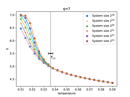
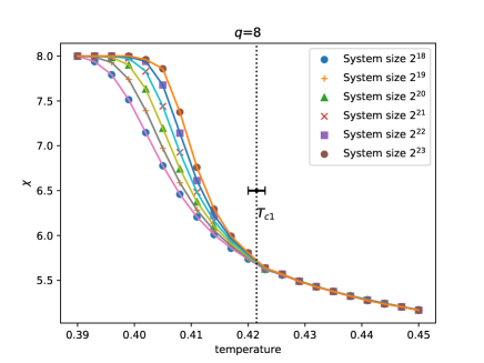
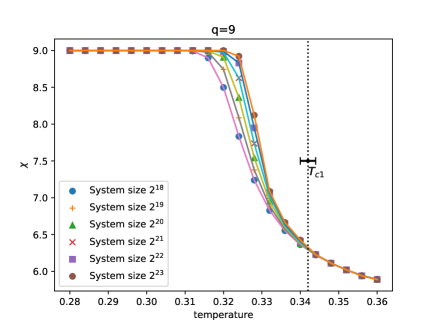
Figure 21: Invariant quantity of for q-state clock model with $q=7,8,9$ around $T_{c1}$

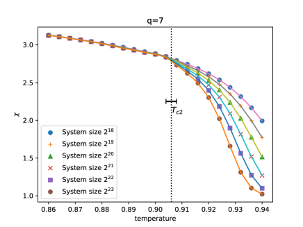
Figure 22: Invariant quantity of for q-state clock model with $q=7,8,9$ around $T_{c2}$

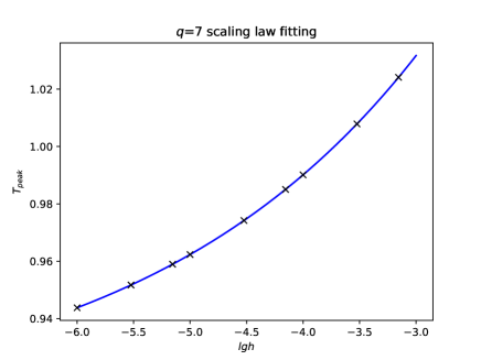
Figure 23: Susceptibility peak temperature versus external field. For $q=7$ model, we find that $T_{c}=0.9065(5),$ $a=0.4198,$ $b=0.1752.$.

Figure 24: Susceptibility peak temperature versus external field. For $q=8$ model, we find that $T_{c}=0.9051(5),$ $a=0.4213$, $b=0.1807$.

Figure 25: Susceptibility peak temperature versus external field. For $q=9$ model, we find that $T_{c}=0.9051(5),$ $a=0.4213$, $b=0.1807$.

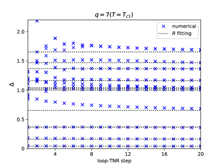
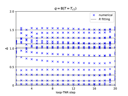
Figure 26: Fitting of scaling dimensions at the critical point $T_{c1}$ for $q=7,8,9$ model, from which we can read the character radius of the compactified boson

Figure 27: Fitting of scaling dimensions at the critical point $T_{c2}$ for q-state clock models with $q=7,8,9$ from which we can read the character radius of the compactified boson

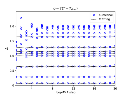
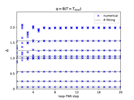
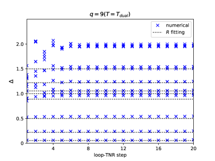
Figure 28: Fitting of scaling dimensions on self-dual point for q-state clock models with $q=7,8,9$

Appendix B Imposing $C_{4}$ rotational symmetry and $Z_{q}$ internal symmetry in loop-TNR algorithm

In this appendix we first give a short review for the loop-TNR algorithm Yang et al. (2017). Then we will discuss how to implement the $C_{4}$ lattice symmetry and the internal $Z_{q}$ symmetry. Loop-TNR method mainly contains the following steps, as shown in Fig. 29. In general, there will be two types of tensors $T_{A}$ and $T_{B}$ on sublattices A and B during the renormaliation process.

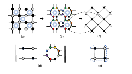
Figure 29: Loop optimization procedure, in step (a), we apply entanglement filtering, and in step (b) we find the optimal $S_{i}$ to minimize cost function as shown (d). Then we trace the indices on the small square marked by the circle. (e) is gauge invariant quantity, which will be used as the overall normalization factor.

$\bullet$ In step (a), we apply entanglement filtering to remove the corner double line(CDL) tensor. The CDL tensor only contains local entanglement and cannot be the fixed point tensor describing critical systems. Ref. Gu and Wen (2009); Yang et al. (2017) gives very clear explanation on how to remove such short range entanglement.

$\bullet$ In step (b), we find 8 rank-3 tensor to form a octagon matrix product state(MPS) to approximate the square MPS, as shown in Fig. 29 (d). We’re aiming to find the optimal choice of those 8 rank-3 tensors $S_{1},S_{2},...S_{8}$ to minimize the cost function in Fig.29 (d), which can be expressed as

$$C\left(S_{1},S_{2},...,S_{8}\right)=\left\|T_{A}\cdot T_{B}\cdot T_{A}\cdot T_{B}-S_{1}\cdot S_{2}\cdot...\cdot S_{8}\right\|^{2}.$$ (24)

Since $S_{1},S_{2},...S_{8}$ are independent variables, we can minimize this cost function with variation method. We denote the two MPS’s in above cost function as:

$$\left|\Psi_{A}\right\rangle = T_{A}\cdot T_{B}\cdot T_{A}\cdot T_{B}$$

$$\left|\Psi_{B}\right\rangle = S_{1}\cdot S_{2}\cdot...\cdot S_{8}$$ (25)

Then, the cost function could be write down as

$$C\left(S_{1},S_{2},...,S_{8}\right)=\left\langle\Psi_{A}|\Psi_{A}\right\rangle+\left\langle\Psi_{B}|\Psi_{B}\right\rangle-\left\langle\Psi_{A}|\Psi_{B}\right\rangle-\left\langle\Psi_{B}|\Psi_{A}\right\rangle.$$ (26)

Taking variation on $S_{1},$ we get

$$\left.\frac{\delta C}{\delta S_{1}^{\dagger}}\right|_{S_{2},S_{3},..S_{8}} = \left\langle\left.\frac{\delta\Psi_{B}}{\delta S_{1}^{\dagger}}\right|\Psi_{B}\right\rangle-\left\langle\left.\frac{\delta\Psi_{B}}{\delta S_{1}^{\dagger}}\right|\Psi_{A}\right\rangle$$ (27)

$$\equiv \left[N_{1}\cdot S_{1}-W_{1}\right].$$

The minimum of $C\left(S_{1}\right)$ is given by the solution of the linear equation:

$$N_{1}\cdot S_{1}=W_{1}.$$ (28)

The cost function (28) and $N_{1}$, $W_{1}$ are illustrated in Fig. 30. After optimizing $S_{1}$, we can go on to the next site, and if we finish the optimization from $S_{1}$ to $S_{8}$, we finish one circle. By repeating this variation optimization, we can minimize the cost function.

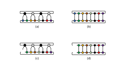
Figure 30: Components of the cost function and its derivative. (a) is $\left\langle\Psi_{A}|\Psi_{B}\right\rangle$. (b) is $\left\langle\Psi_{B}|\Psi_{B}\right\rangle$. (c) and (d) are the quantity $W_{1}$ and $N_{1}$ in (28), respectively.

$\bullet$ After minimizing the cost function, we trace the inner indices in the small circles, as shown in Fig. 29 (b), and get the coarse-grained tensor $T_{A}^{\prime}$ and $T_{B}^{\prime},$ as in Fig. 29 (c). Compared with the original tensor network, we find the tensor network composed of the renormalized tensor elements $T_{A}^{\prime}$ and $T_{B}^{\prime}$ (a) rotates an angle of $\pi/4$ and (b) the system size of the new network reduced to be half of the original. Then, we can start the new RG step from this tensor network

$\bullet$ We will normalize the tensor $T_{A}$ and $T_{B}$ in every RG step with the normalization factor as shown in Fig. 29 (e).

B.1 loop-TNR with $C_{4}$ lattice symmetry

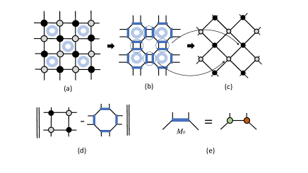
Figure 31: Loop-TNR algorithm with $C_{4}$ lattice symmetry is similar with usual loop-TNR. Notice that the cost function in this case is nonlinear, so we need to use nonlinear optimization algorithm, such as conjugate gradient method.

To keep the lattice symmetry in the renormalization process, we need to find a octagon MPS with $C_{4}$ symmetry when minimizing the cost function in Fig. 31 (d). We can construct this octagon MPS with the rank-4 block tensor $M_{ijkl}$, as shown in Fig. 31 (b). Then we can use the conjugate gradient method to minimize the cost function:

$$C=\left\|T_{A}\cdot T_{B}\cdot T_{A}\cdot T_{B}-M\cdot M\cdot M\cdot M\right\|^{2}.$$ (29)

After the optimization, we can use tensor $M$ to build the renormalized tensor $T_{A}^{\prime},T_{B}^{\prime}$, as shown in Fig.31 (c)

$$T_{ruld}^{A\prime} = \underset{ij}{\sum}M_{ijrd}M_{jilu}$$

$$T_{ruld}^{B\prime} = \underset{ij}{\sum}M_{ijld}M_{jiru}.$$ (30)

Since the octagon network has $C_{4}$ symmetry, the coarse-grained tensor network on the square lattice marked by blue circle has the same $C_{4}$ symmetries.

The initial value of the tensor $M$ is very important for the numerical accuracy. We can decompose tensor $T_{A}$ and $T_{B}$ by SVD method

$$T_{ruld}^{A} \approx \underset{x}{\sum}S_{ldx}^{1}S_{rux}^{2}=\underset{x}{\sum}S_{rux}^{1}S_{ldx}^{2}$$

$$T_{ruld}^{B} \approx \underset{x}{\sum}S_{ulx}^{1}S_{drx}^{2}=\underset{x}{\sum}S_{drx}^{1}S_{ulx}^{2}.$$ (31)

Thus, the initial $M$ is could be constructed as Fig. 31 (e), with

$$M_{ijkl}^{0}=\underset{x}{\sum}S_{ixk}^{1}S_{xjl}^{2}.$$ (32)

By keeping $C_{4}$ lattice symmetries in each iteration step, we have partially fixed the gauge of the building block $M$, which would be very important for studying the structure of the fixed point tensor.

B.2 loop-TNR with $Z(q)$ symmetry in Hamiltonian

As the original tensor element of $q$-state model $T_{ijkl}$ contains $Z\left(q\right)$ symmetry, we can keep such a symmetry for every step in the loop-TNR algorithm. As $Z\left(q\right)$ is a cyclic group, which contains group elements $\left\{I,g,g^{2},...g^{q-1}\right\}$, and the generator $g$ has the $q$-dimension faithful representation

$$G_{q}=\left(\begin{array}[]{cccccc}0&0&0&...&0&1\\ 1&0&0&...&0&0\\ 0&1&0&...&0&0\\ 0&0&1&...&0&0\\ ...&...&...&...&...&...\\ 0&0&0&...&1&0\end{array}\right).$$ (33)

It is easy to check that:

$$T_{ruld}^{\prime} = \underset{r^{\prime}u^{\prime}l^{\prime}d^{\prime}}{\sum}\left[G_{q}\right]_{rr^{\prime}}\left[G_{q}\right]_{uu^{\prime}}\left[G_{q}\right]_{ll^{\prime}}\left[G_{q}\right]_{dd^{\prime}}T_{r^{\prime}u^{\prime}l^{\prime}d^{\prime}}$$ (34)

$$= T_{ruld}.$$

In order to find out all the irreducible representation of the $Z_{q}$ symmetry, we can just do eigenvalue decomposition for $G_{q}$,

$$G_{q}=V\Lambda V^{-1},$$ (35)

with eigenvalues $\Lambda_{nn}=\lambda_{n}=e^{2\pi in/q},n\in\{0,1,2,...,q-1\}$, and the components of the matrix $V$ is given by:

$$V_{mn}=\frac{e^{2\pi imn/q}}{\sqrt{q}},m,n\in\{0,1,2,...,q-1\}.$$ (36)

Such that:

$$G_{q}=V^{-1}\Lambda^{-1}V.$$ (37)

Then, we define two tensors:

$$T^{A}_{ruld} = \underset{r^{\prime}u^{\prime}l^{\prime}d^{\prime}}{\sum}\left[V^{-1}\right]_{rr^{\prime}}\left[V^{-1}\right]_{uu^{\prime}}\left[V^{-1}\right]_{ll^{\prime}}\left[V^{-1}\right]_{dd^{\prime}}T_{r^{\prime}u^{\prime}l^{\prime}d^{\prime}}$$

$$T^{B}_{ruld} = \underset{r^{\prime}u^{\prime}l^{\prime}d^{\prime}}{\sum}V_{rr^{\prime}}V_{uu^{\prime}}V_{ll^{\prime}}V_{dd^{\prime}}T_{r^{\prime}u^{\prime}l^{\prime}d^{\prime}}.$$ (38)

Obviously, tensor $T^{A}$ and $T^{B}$ form the same tensor network with $T$. In the new basis tensors $T^{A}$ and $T^{B}$ satisfy:

$$T^{A}_{ruld} = \lambda_{r}\lambda_{u}\lambda_{l}\lambda_{d}T^{A}_{ruld}$$

$$T^{B}_{ruld} = \lambda_{r}^{-1}\lambda_{u}^{-1}\lambda_{l}^{-1}\lambda_{d}^{-1}T^{B}_{ruld},$$ (39)

which implies that $T^{A}_{ruld}$ and $T^{B}_{ruld}$ only have non-zero components when $r+u+l+d\equiv 0\left(\text{mod }q\right)$. Thus, tensors $T^{A}$ and $T^{B}$ are block diagonalized. It turns out that if we keep such block diagonalized property during RG process, i.e., in every RG step, we keep $r+u+l+d\equiv 0\left(\text{mod }q\right)$, $Z\left(q\right)$ symmetry is preserved during loop-TNR process. In particular, we can keep $D_{cut}=nq$(where $n$ is an arbitrary integer), such that we can always construct a dimension $nq$ by $nq$ block diagonalized matrix $\Lambda^{\prime}$

$$\Lambda^{\prime}=\left(\begin{array}[]{cccc}\Lambda&\mathbf{0}&...&\mathbf{0}\\ \mathbf{0}&\Lambda&...&\mathbf{0}\\ ...&...&...&...\\ \mathbf{0}&\mathbf{0}&...&\Lambda\end{array}\right).$$ (40)

Obviously, $\Lambda^{\prime}$ is a representation of $Z\left(q\right)$ symmetry. So that $Z\left(q\right)$ symmetry is kept.

References

- Berezinskii (1971) V. Berezinskii, Sov. Phys. JETP 32, 493 (1971).
- Kosterlitz and Thouless (1972) J. Kosterlitz and D. Thouless, Journal of Physics C: Solid State Physics 5, L124 (1972).
- Kosterlitz and Thouless (1973) J. Kosterlitz and D. Thouless, Journal of Physics C: Solid State Physics 6, 1181 (1973).
- José et al. (1977) J. José, L. Kadanoff, S. Kirkpatrick, and D. Nelson, Phys. Rev. B 16, 1217 (1977).
- Wiegmann (1978) P. Wiegmann, Journal of Physics C: Solid State Physics 11, 1583 (1978).
- Matsuo and Nomura (2006) H. Matsuo and K. Nomura, Journal of Physics A: Mathematical and General 39, 2953 (2006).
- Tobochnik (1982) J. Tobochnik, Phys. Rev. B 26, 6201 (1982).
- Baek et al. (2009) S.-K. Baek, P. Minnhagen, and B. Kim, Phys. Rev. E 80, 060101 (2009).
- Baek and Minnhagen (2010) S. Baek and P. Minnhagen, Phys. Rev. E 82, 031102 (2010).
- Kumano et al. (2013) Y. Kumano, K. Hukushima, Y. Tomita, and M. Oshikawa, Phys. Rev. B 88, 104427 (2013).
- Chatelain (2014) C. Chatelain, J. Stat. Mech. 2014, 11022 (2014).
- Krcmar et al. (2016) R. Krcmar, A. Gendiar, and T. Nishino, arXiv:1612.07611 (2016).
- Chen et al. (2017) J. Chen, H.-J. Liao, H.-D. Xie, X.-J. Han, R.-Z. Huang, S. Cheng, Z.-C. Wei, Z.-Y. Xie, and T. Xiang, Chinese Physics Letters 34, 050503 (2017).
- Kim (2017) D.-H. Kim, Phys. Rev. E 96, 052130 (2017).
- Chen et al. (2018) Y. Chen, Z.-Y. Xie, and J.-F. Fu, Chin. Phys. B 27, 080503 (2018).
- Hong and Kim (2020) S. Hong and D.-H. Kim, Phys. Rev. E 101, 012124 (2020).
- Challa and Landau (1986) M. Challa and D. Landau, Phys. Rev. B 33, 437 (1986).
- Zhang and Ji (1990) J.-B. Zhang and D.-R. Ji, Phys. Lett. A 151, 469 (1990).
- Yamagata and Ono (1991) A. Yamagata and I. Ono, Journal of Physics A: Mathematical and General 24, 265 (1991).
- Tomita and Okabe (2002) Y. Tomita and Y. Okabe, Phys. Rev. B 65, 184405 (2002).
- Hwang (2009) C.-O. Hwang, Phys. Rev. E 80, 042103 (2009).
- Brito et al. (2010) A. Brito, J. Redinz, and J. Plascak, Phys. Rev. E 81, 031130 (2010).
- Borisenko et al. (2011) O. Borisenko, G. Cortese, R. Fiore, M. Gravina, and A. Papa, Phys. Rev. E 83, 041120 (2011).
- Borisenko et al. (2012) O. Borisenko, V. Chelnokov, G. Cortese, R. Fiore, M. Gravina, and A. Papa, Phys. Rev. E 85, 021114 (2012).
- Wu et al. (2012) R. P.-H. Wu, V.-C. Lo, and H.-T. Huang, J. Appl. Phys. 112, 063924 (2012).
- Baek et al. (2013) S.-K. Baek, H. Mäkelä, P. Minnhagen, and B.-J. Kim, Phys. Rev. E 88, 012125 (2013).
- Chatterjee et al. (2018) S. Chatterjee, S. Puri, and R. Paul, Phys. Rev. E 98, 032109 (2018).
- Surungan et al. (2019) T. Surungan, S. Masuda, Y. Komura, and Y. Okabe, J. Phys. A 52, 275002 (2019).
- Li et al. (2020) Z.-Q. Li, L.-P. Yang, Z.-Y. Xie, H.-H. Tu, H.-J. Liao, and T. Xiang, Phys. Rev. E 101, 060105 (2020).
- Levin and Nave (2007) M. Levin and C. Nave, Phys. Rev. Lett. 99, 120601 (2007).
- Gu and Wen (2009) Z.-C. Gu and X.-G. Wen, Phys. Rev. B 80, 155131 (2009).
- Yang et al. (2017) S. Yang, Z.-C. Gu, and X.-G. Wen, Phys. Rev. Lett. 118, 110504 (2017).
- Xie et al. (2009) Z.-Y. Xie, H.-C. Jiang, Q.-J. N. Chen, Z.-Y. Weng, and T. Xiang, Phys. Rev. Lett. 103, 160601 (2009).
- Xie et al. (2012) Z. Y. Xie, J. Chen, M. P. Qin, J. W. Zhu, L. P. Yang, and T. Xiang, Phys. Rev. B 86, 045139 (2012).
- Janke (1997) W. Janke, Phys. Rev. B 55, 3580 (1997).
- Kramers and Wannier (1941a) H. Kramers and G. Wannier, Phys. Rev. 60, 252 (1941a).
- Yu et al. (2014) J.-F. Yu, Z.-Y. Xie, Y. Meurice, Y.-Z. Liu, A. Denbleyker, H.-Y. Zou, M.-P. Qin, J. Chen, and T. Xiang, Phys. Rev. E 89, 013308 (2014).
- Kramers and Wannier (1941b) H. Kramers and G. Wannier, Phys. Rev. 60, 263 (1941b).
- Zamolodchikov and Monastyrski (1979) A. Zamolodchikov and M. Monastyrski, JETP Lett 2, 196511 (1979).
- Bhattacharyya et al. (2018) A. Bhattacharyya, L.-Y. Hung, Y. Lei, and W. Li, Journal of High Energy Physics 01, 139 (2018).