Renormalized Oscillation Theory for Singular Linear Hamiltonian Systems

Abstract

Working with a general class of linear Hamiltonian systems with at least one singular boundary condition, we show that renormalized oscillation results can be obtained in a natural way through consideration of the Maslov index associated with appropriately chosen paths of Lagrangian subspaces of $\mathbb{C}^{2n}$. This extends previous work by the authors for regular linear Hamiltonian systems.

1 Introduction

We consider linear Hamiltonian systems

$$Jy^{\prime}=(B_{0}(x)+\lambda B_{1}(x))y;\quad y(x;\lambda)\in\mathbb{C}^{2n},\quad n\in\{1,2,\dots\},$$ (1.1)

where $J$ denotes the standard symplectic matrix

$$J=\begin{pmatrix}0_{n}&-I_{n}\\ I_{n}&0_{n}\end{pmatrix}.$$

We specify (1.1) on intervals $(a,b)$, with $-\infty\leq a<b\leq+\infty$, and we assume throughout that $B_{0},B_{1}\in L^{1}_{\operatorname{loc}}((a,b),\mathbb{C}^{2n\times 2n})$, and additionally that $B_{0}(x)$ and $B_{1}(x)$ are both self-adjoint for a.e. $x\in(a,b)$. For convenient reference, we refer to these assumptions as Assumptions (A). In addition, we make the following Atkinson-type positivity assumption.

(B) If $y(\cdot;\lambda)\in\operatorname{AC}_{\operatorname{loc}}((a,b),\mathbb{C}^{2n})$ is any non-trivial solution of (1.1), then

$$\int_{c}^{d}(B_{1}(x)y(x;\lambda),y(x;\lambda))dx>0,$$

for all $[c,d]\subset(a,b)$. (Here, $\operatorname{AC}_{\operatorname{loc}}$ denotes local absolute continuity, and $(\cdot,\cdot)$ denotes the usual inner product on $\mathbb{C}^{2n}$.)

Our goal is to associate (1.1) with one or more self-adjoint operators $\mathcal{L}$ (see Lemma 1.1 below), and to use renormalized oscillation theory to count the number of eigenvalues $\mathcal{N}([\lambda_{1},\lambda_{2}))$ that each such operator has on a given interval $[\lambda_{1},\lambda_{2})\subset\mathbb{R}$ for which the closure $[\lambda_{1},\lambda_{2}]$ has empty intersection with the essential spectrum of the operator. We will formulate our results for two cases: (1) when $x=a$ is a regular boundary point for (1.1); and (2) when $x=a$ is a singular boundary point for (1.1). (We take (1.1) to be singular at $x=b$ in both cases; the case in which (1.1) is regular at both endpoints has been analyzed in [22].) The case in which (1.1) is regular at $x=a$ corresponds with the following additional assumption.

(A)^′ The value $a$ is finite, and for any $c\in(a,b)$, we have $B_{0},B_{1}\in L^{1}((a,c),\mathbb{C}^{2n\times 2n})$.

Our starting point will be to specify an appropriate Hilbert space to work in, and for this we follow [27]. We denote by $\tilde{L}^{2}_{B_{1}}((a,b),\mathbb{C}^{2n})$ the set of all Lebesgue measureable functions $f$ defined on $(a,b)$ so that

$$\|f\|_{B_{1}}:=\Big{(}\int_{a}^{b}(B_{1}(x)f(x),f(x))dx\Big{)}^{1/2}<\infty.$$

Correspondingly, we denote by $\mathcal{Z}_{B_{1}}$ the subset of $\tilde{L}^{2}_{B_{1}}((a,b),\mathbb{C}^{2n})$ comprising elements $f\in\tilde{L}^{2}_{B_{1}}((a,b),\mathbb{C}^{2n})$ so that $\|f\|_{B_{1}}=0$. Our Hilbert space will be the quotient space,

$$L^{2}_{B_{1}}((a,b),\mathbb{C}^{2n})=\tilde{L}^{2}_{B_{1}}((a,b),\mathbb{C}^{2n})/\mathcal{Z}_{B_{1}}.$$

I.e., two functions $f,g\in L^{2}_{B_{1}}((a,b),\mathbb{C}^{2n})$ are equivalent if and only if $\|f-g\|_{B_{1}}=0$. With this specification, $\|\cdot\|_{B_{1}}$ is a norm on $L^{2}_{B_{1}}((a,b),\mathbb{C}^{2n})$. We equip $L^{2}_{B_{1}}((a,b),\mathbb{C}^{2n})$ with the inner product

$$\langle f,g\rangle_{B_{1}}:=\int_{a}^{b}(B_{1}(x)f(x),g(x))dx.$$

In all of these specifications, we emphasize that $B_{1}(x)$ need not be an invertible matrix.

We now introduce a maximal operator associated with (1.1).

Definition 1.1.

(i) We denote by $\mathcal{D}_{M}$ the collection of all

$$y\in\operatorname{AC}_{\operatorname{loc}}((a,b),\mathbb{C}^{2n})\cap L^{2}_{B_{1}}((a,b),\mathbb{C}^{2n})$$

for which there exists some $f\in L^{2}_{B_{1}}((a,b),\mathbb{C}^{2n})$ so that

$$Jy^{\prime}-B_{0}(x)y=B_{1}(x)f,$$

for a.e. $x\in(a,b)$. We will refer to $\mathcal{D}_{M}$ as the maximal domain, and we note that $f$ is uniquely determined in $L^{2}_{B_{1}}((a,b),\mathbb{C}^{2n})$. (If $f$ and $g$ are two functions associated with the same $y\in\mathbf{\mathcal{D}}_{M}$, then $B_{1}(x)(f-g)=0$ for a.e. $x\in(a,b)$, so that $f=g$ in $L^{2}_{B_{1}}((a,b),\mathbb{C}^{2n})$.)

(ii) We define the maximal operator $\mathcal{L}_{M}:L^{2}_{B_{1}}((a,b),\mathbb{C}^{2n})\to L^{2}_{B_{1}}((a,b),\mathbb{C}^{2n})$ as the map taking a given $y\in\mathcal{D}_{M}$ to the unique $f\in L^{2}_{B_{1}}((a,b),\mathbb{C}^{2n})$ guaranteed by the definition of $\mathcal{D}_{M}$. We note particularly that $y(\cdot;\lambda)\in\mathcal{D}_{M}$ solves (1.1) iff and only if $\mathcal{L}_{M}y=\lambda y$ a.e. in $(a,b)$.

The following terminology will be convenient for the discussion.

Definition 1.2.

We say that a solution $y(\cdot;\lambda)\in\operatorname{AC}_{\operatorname{loc}}((a,b),\mathbb{C}^{2n})$ of (1.1) lies left in $(a,b)$ if for any $c\in(a,b)$, the restriction of $y(\cdot;\lambda)$ to $(a,c)$ is in $L^{2}_{B_{1}}((a,c),\mathbb{C}^{2n})$. Likewise, we say that a solution $y(\cdot;\lambda)\in\operatorname{AC}_{\operatorname{loc}}((a,b),\mathbb{C}^{2n})$ of (1.1) lies right in $(a,b)$ if for any $c\in(a,b)$, the restriction of $y(\cdot;\lambda)$ to $(c,b)$ is in $L^{2}_{B_{1}}((c,b),\mathbb{C}^{2n})$. For each fixed $\lambda\in\mathbb{C}$ we will denote by $m_{a}(\lambda)$ the dimension of the space of solutions to (1.1) that lie left in $(a,b)$, and we will denote by $m_{b}(\lambda)$ the dimension of the space of solutions to (1.1) that lie right in $(a,b)$.

We will show in Section 2 that if Assumptions (A) and (B) hold, then for any $\lambda\in\mathbb{C}\backslash\mathbb{R}$, (1.1) admits at least $n$ solutions that lie left in $(a,b)$ and at least $n$ solutions that lie right in $(a,b)$. According to Theorem V.2.2 in [27], $m_{a}(\lambda)$ and $m_{b}(\lambda)$ are both constant for all $\lambda$ with $\textrm{Im}\,\lambda>0$, and the same statement is true for $\textrm{Im}\,\lambda<0$. In the event that $B_{0}(x)$ and $B_{1}(x)$ have real-valued entries for a.e. $x\in(a,b)$, it is furthermore the case that $m_{a}(\lambda)$ and $m_{b}(\lambda)$ are both constant for all $\lambda\in\mathbb{C}\backslash\mathbb{R}$. (See our Remark 2.1.) We will allow $B_{0}(x)$ and $B_{1}(x)$ to have complex-valued entries, but we will make the following consistency assumption:

(C) The values $m_{a}(\lambda)$ and $m_{b}(\lambda)$ are both constant for all $\lambda\in\mathbb{C}\backslash\mathbb{R}$. We denote these common values $m_{a}$ and $m_{b}$.

In the event that Assumption (A)^′ also holds, it’s clear that $m_{a}(\lambda)=2n$ for all $\lambda\in\mathbb{C}$. In the terminology of our next definition, this means that under Assumption (A)^′, (1.1) is in the limit circle case at $x=a$. In this case, Assumption (C) holds immediately for $x=a$, with $m_{a}=2n$.

Definition 1.3.

If $m_{a}=n$, we say that (1.1) is in the limit point case at $x=a$, and if $m_{a}=2n$, we say that (1.1) is in the limit circle case at $x=a$. If $m_{a}\in(n,2n)$, we say that (1.1) is in the limit-$m_{a}$ case at $x=a$. Analogous specifications are made at $x=b$.

Under Assumptions (A), (B), and (C), we will show that by taking an appropriate selection of solutions that lie left in $(a,b)$, $\{u^{a}_{j}(x;\lambda)\}_{j=1}^{n}$, and an appropriate selection of solutions that lie right in $(a,b)$, $\{u^{b}_{j}(x;\lambda)\}_{j=1}^{n}$, we can specify the domain of a self-adjoint restriction of $\mathcal{L}_{M}$, which we will denote $\mathcal{L}$. For the purposes of this introduction, we will sum this development up in the following lemma, for which we denote by $U^{a}(x;\lambda)$ the matrix comprising the vector functions $\{u^{a}_{j}(x;\lambda)\}_{j=1}^{n}$ as its columns, and by $U^{b}(x;\lambda)$ the matrix comprising the vector functions $\{u^{b}_{j}(x;\lambda)\}_{j=1}^{n}$ as its columns. The selection process is described in detail in Section 2; see especially the summary in Remark 2.3.

Lemma 1.1.

(i) Let Assumptions (A), (B), and (C) hold, and let $\lambda_{0}\in\mathbb{C}\backslash\mathbb{R}$ be fixed. Then there exists a selection of solutions $\{u^{a}_{j}(x;\lambda_{0})\}_{j=1}^{n}$ to (1.1) that lie left in $(a,b)$, along with a selection of solutions $\{u^{b}_{j}(x;\lambda_{0})\}_{j=1}^{n}$ to (1.1) that lie right in $(a,b)$ so that the restriction of $\mathcal{L}_{M}$ to the domain

$$\mathcal{D}:=\{y\in\mathcal{D}_{M}:\lim_{x\to a^{+}}U^{a}(x;\lambda_{0})^{*}Jy(x)=0,\quad\lim_{x\to b^{-}}U^{b}(x;\lambda_{0})^{*}Jy(x)=0\}$$

is a self-adjoint operator. We will denote this operator $\mathcal{L}$.

(ii) Let Assumptions (A), (A)^′, (B), and (C) hold, and let $\lambda_{0}\in\mathbb{C}\backslash\mathbb{R}$ be fixed. In addition, let $\alpha\in\mathbb{C}^{n\times 2n}$ denote any fixed matrix satisfying $\operatorname{rank}\alpha=n$ and $\alpha J\alpha^{*}=0$. Then there exists a selection of solutions $\{u^{b}_{j}(x;\lambda_{0})\}_{j=1}^{n}$ to (1.1) that lie right in $(a,b)$ so that the restriction of $\mathcal{L}_{M}$ to the domain

$$\mathcal{D}^{\alpha}:=\{y\in\mathcal{D}_{M}:\alpha y(a)=0,\quad\lim_{x\to b^{-}}U^{b}(x;\lambda_{0})^{*}Jy(x)=0\}$$

is a self-adjoint operator. We will denote this operator $\mathcal{L}^{\alpha}$.

In order to set some notation and terminology for this discussion, we make the following standard definitions.

Definition 1.4.

We denote by $\rho(\mathcal{L})$ the usual resolvent set

$$\rho(\mathcal{L}) :=\{\lambda\in\mathbb{C}:(\mathcal{L}-\lambda I)^{-1}:L^{2}_{B_{1}}((a,b),\mathbb{C}^{n})\to L^{2}_{B_{1}}((a,b),\mathbb{C}^{n})$$

$$\quad\quad\quad\textrm{ is a bounded linear operator}\},$$

and we denote by $\sigma(\mathcal{L})$ the spectrum of $\mathcal{L}$, $\sigma(\mathcal{L}):=\mathbb{C}\backslash\rho(\mathcal{L})$. In addition, we define the point spectrum of $\mathcal{L}$ to the be collection of eigenvalues,

$$\sigma_{p}(\mathcal{L}):=\{\lambda\in\mathbb{C}:\mathcal{L}y=\lambda y\textrm{ for some }y\in\mathcal{D}\backslash\{0\}\},$$

and we define the essential spectrum of $\mathcal{L}$, denoted $\sigma_{\operatorname{ess}}(\mathcal{L})$ to be the collection of all $\lambda\in\mathbb{C}$ so that $\lambda\notin\rho(\mathcal{L})$ and $\lambda$ is not an isolated eigenvalue of $\mathcal{L}$ with finite multiplicity. Finally, we define the discrete spectrum of $\mathcal{L}$ to be $\sigma_{\rm discrete}(\mathcal{L})=\sigma(\mathcal{L})\backslash\sigma_{\operatorname{ess}}(\mathcal{L})$. We will use precisely the same definitions for $\mathcal{L}^{\alpha}$, with $\mathcal{D}$ replaced by $\mathcal{D}^{\alpha}$.

Our primary tool for this analysis will be the Maslov index, and as a starting point for a discussion of this object, we define what we will mean by a Lagrangian subspace of $\mathbb{C}^{2n}$.

Definition 1.5.

We say $\ell\subset\mathbb{C}^{2n}$ is a Lagrangian subspace of $\mathbb{C}^{2n}$ if $\ell$ has dimension $n$ and

$$(Ju,v)=0,$$ (1.2)

for all $u,v\in\ell$. In addition, we denote by $\Lambda(n)$ the collection of all Lagrangian subspaces of $\mathbb{C}^{2n}$, and we will refer to this as the Lagrangian Grassmannian.

Remark 1.1.

Following the convention of Arnol’d’s foundational paper [3], the notation $\Lambda(n)$ is often used to denote the Lagrangian Grassmannian associated with $\mathbb{R}^{2n}$. Our expectation is that it can be used in the current setting of $\mathbb{C}^{2n}$ without confusion. We note that the Lagrangian Grassmannian associated with $\mathbb{C}^{2n}$ has been considered by a number of authors, including (ordered by publication date) Bott [10], Kostrykin and Schrader [26], Arnol’d [4], and Schulz-Baldes [39, 40]. It is shown in all of these references that $\Lambda(n)$ is homeomorphic to the set of $n\times n$ unitary matrices $U(n)$, and in [39, 40] the relationship is shown to be diffeomorphic. It is also shown in [39] that the fundamental group of $\Lambda(n)$ is isomorphic to the integers $\mathbb{Z}$.

Any Lagrangian subspace of $\mathbb{C}^{2n}$ can be spanned by a choice of $n$ linearly independent vectors in $\mathbb{C}^{2n}$. We will generally find it convenient to collect these $n$ vectors as the columns of a $2n\times n$ matrix $\mathbf{X}$, which we will refer to as a frame for $\ell$. Moreover, we will often coordinatize our frames as $\mathbf{X}={X\choose Y}$, where $X$ and $Y$ are $n\times n$ matrices. Following [15] (p. 274), we specify a metric on $\Lambda(n)$ in terms of appropriate orthogonal projections. Precisely, let $\mathcal{P}_{i}$ denote the orthogonal projection matrix onto $\ell_{i}\in\Lambda(n)$ for $i=1,2$. I.e., if $\mathbf{X}_{i}$ denotes a frame for $\ell_{i}$, then $\mathcal{P}_{i}=\mathbf{X}_{i}(\mathbf{X}_{i}^{*}\mathbf{X}_{i})^{-1}\mathbf{X}_{i}^{*}$. We take our metric $d$ on $\Lambda(n)$ to be defined by

$$d(\ell_{1},\ell_{2}):=\|\mathcal{P}_{1}-\mathcal{P}_{2}\|,$$

where $\|\cdot\|$ can denote any matrix norm. We will say that a path of Lagrangian subspaces $\ell:\mathcal{I}\to\Lambda(n)$ is continuous provided it is continuous under the metric $d$.

Suppose $\ell_{1}(\cdot),\ell_{2}(\cdot)$ denote continuous paths of Lagrangian subspaces $\ell_{i}:\mathcal{I}\to\Lambda(n)$, $i=1,2$, for some parameter interval $\mathcal{I}$ (not necessarily closed and bounded). The Maslov index associated with these paths, which we will denote $\operatorname{Mas}(\ell_{1},\ell_{2};\mathcal{I})$, is a count of the number of times the paths $\ell_{1}(\cdot)$ and $\ell_{2}(\cdot)$ intersect, counted with both multiplicity and direction. (In this setting, if we let $t_{*}$ denote the point of intersection (often referred to as a conjugate point), then multiplicity corresponds with the dimension of the intersection $\ell_{1}(t_{*})\cap\ell_{2}(t_{*})$; a precise definition of what we mean in this context by direction will be given in Section 3.)

In order to formulate our results for the case in which (1.1) is regular at $x=a$, we introduce the $2n\times n$ matrix solution $\mathbf{X}_{\alpha}(x;\lambda)$ to the initial value problem

$$J\mathbf{X}_{\alpha}^{\prime} =(B_{0}(x)+\lambda B_{1}(x))\mathbf{X}_{\alpha}$$ (1.3)

$$\mathbf{X}_{\alpha} (a;\lambda)=J\alpha^{*}.$$

Under our assumptions (A), (A)^′, we can conclude that for each $\lambda\in\mathbb{C}$, $\mathbf{X}_{\alpha}(\cdot;\lambda)\in AC_{\operatorname{loc}}([a,b),\mathbb{C}^{2n\times n})$. In addition, $\mathbf{X}_{\alpha}\in C([a,b)\times\mathbb{C},\mathbb{C}^{2n\times n})$, and $\mathbf{X}_{\alpha}(x;\cdot)$ is analytic in $\lambda$. (See, for example, [46].) As shown in [19], for each pair $(x,\lambda)\in[a,b)\times\mathbb{R}$, $\mathbf{X}_{\alpha}(x;\lambda)$ is the frame for a Lagrangian subspace of $\mathbb{C}^{2n}$, which we will denote $\ell_{\alpha}(x;\lambda)$. (In [19], the authors make slightly stronger assumptions on $B_{0}(x)$ and $B_{1}(x)$, but their proof carries over immediately into our setting.)

For the frame associated with the right endpoint, we let $[\lambda_{1},\lambda_{2}]$, $\lambda_{1}<\lambda_{2}$, be such that $[\lambda_{1},\lambda_{2}]\cap\sigma_{\operatorname{ess}}(\mathcal{L}^{\alpha})=\emptyset$. In Section 2, we will show that for each $\lambda\in[\lambda_{1},\lambda_{2}]$, there exists a $2n\times n$ matrix solution $\mathbf{X}_{b}(x;\lambda)$ to the ODE

$$J\mathbf{X}_{b}^{\prime}= (B_{0}(x)+\lambda B_{1}(x))\mathbf{X}_{b}$$ (1.4)

$$\lim_{x\to b^{-}} U^{b}(x;\lambda_{0})^{*}J\mathbf{X}_{b}(x;\lambda)=0,$$

where the matrix $U^{b}(x;\lambda_{0})$ is described in Lemma 1.1 (and the paragraph leading into that lemma). In addition, we will check that for each pair $(x,\lambda)\in[a,b)\times[\lambda_{1},\lambda_{2}]$, $\mathbf{X}_{b}(x;\lambda)$ is the frame for a Lagrangian subspace of $\mathbb{C}^{2n}$, which we will denote $\ell_{b}(x;\lambda)$, and we will also check that $\ell_{b}\in C([a,b)\times[\lambda_{1},\lambda_{2}],\Lambda(n))$.

In Section 4, we will establish the following theorem.

Theorem 1.1.

Let Assumptions (A), (A)^′, (B), and (C) hold, and assume that for some pair $\lambda_{1},\lambda_{2}\in\mathbb{R}$, $\lambda_{1}<\lambda_{2}$, we have $\sigma_{\operatorname{ess}}(\mathcal{L}^{\alpha})\cap[\lambda_{1},\lambda_{2}]=\emptyset$. If $\ell_{\alpha}(\cdot;\lambda_{1})$ and $\ell_{b}(\cdot;\lambda_{2})$ denote the paths of Lagrangian subspaces of $\mathbb{C}^{2n}$ constructed just above, and $\mathcal{N}^{\alpha}([\lambda_{1},\lambda_{2}))$ denotes a count of the number of eigenvalues $\mathcal{L}^{\alpha}$ has on the interval $[\lambda_{1},\lambda_{2})$, then

$$\mathcal{N}^{\alpha}([\lambda_{1},\lambda_{2}))\geq\operatorname{Mas}(\ell_{\alpha}(\cdot;\lambda_{1}),\ell_{b}(\cdot;\lambda_{2});[a,b)).$$ (1.5)

If additionally $\lambda_{1},\lambda_{2}\notin\sigma_{p}(\mathcal{L}^{\alpha})$, then we have equality in (1.5).

In the case that (A)^′ doesn’t hold, so that (1.1) is singular at $x=a$, we let $[\lambda_{1},\lambda_{2}]$, $\lambda_{1}<\lambda_{2}$, be such that $[\lambda_{1},\lambda_{2}]\cap\sigma_{\operatorname{ess}}(\mathcal{L})=\emptyset$. We will show in Section 2 that for each $\lambda\in[\lambda_{1},\lambda_{2}]$ there exists a $2n\times n$ matrix solution $\mathbf{X}_{a}(x;\lambda)$ to the ODE

$$J\mathbf{X}_{a}^{\prime}= (B_{0}(x)+\lambda B_{1}(x))\mathbf{X}_{a}$$ (1.6)

$$\lim_{x\to a^{+}} U^{a}(x;\lambda_{0})^{*}J\mathbf{X}_{a}(x;\lambda)=0,$$

where the matrix $U^{a}(x;\lambda_{0})$ is described in Lemma 1.1 (and the paragraph leading into that lemma). In addition, we will check that for each pair $(x,\lambda)\in[a,b)\times[\lambda_{1},\lambda_{2}]$, $\mathbf{X}_{a}(x;\lambda)$ is the frame for a Lagrangian subspace of $\mathbb{C}^{2n}$, which we will denote $\ell_{a}(x;\lambda)$, and that $\ell_{a}\in C((a,b)\times[\lambda_{1},\lambda_{2}],\Lambda(n))$.

In Section 4, we will establish the following theorem.

Theorem 1.2.

Let Assumptions (A), (B), and (C) hold, and assume that for some pair $\lambda_{1},\lambda_{2}\in\mathbb{R}$, $\lambda_{1}<\lambda_{2}$, we have $\sigma_{\operatorname{ess}}(\mathcal{L})\cap[\lambda_{1},\lambda_{2}]=\emptyset$. If $\ell_{a}(\cdot;\lambda_{1})$ and $\ell_{b}(\cdot;\lambda_{2})$ denote the paths of Lagrangian subspaces of $\mathbb{C}^{2n}$ constructed just above, and $\mathcal{N}([\lambda_{1},\lambda_{2}))$ denotes a count of the number of eigenvalues $\mathcal{L}$ has on the interval $[\lambda_{1},\lambda_{2})$, then

$$\mathcal{N}([\lambda_{1},\lambda_{2}))\geq\operatorname{Mas}(\ell_{a}(\cdot;\lambda_{1}),\ell_{b}(\cdot;\lambda_{2});(a,b)).$$ (1.7)

If additionally $\lambda_{1},\lambda_{2}\notin\sigma_{p}(\mathcal{L})$, then we have equality in (1.7).

In order to relate our results to previous work on renormalized oscillation theory, we observe that in some cases the Maslov index can be expressed as a sum of nullities for certain evolving matrix Wronskians. To understand this, we first specify the following terminology: for two paths of Lagrangian subspaces $\ell_{1},\ell_{2}:\mathcal{I}\to\Lambda(n)$, we say that the evolution of the pair $\ell_{1},\ell_{2}$ is monotonic provided all intersections occur in the same direction. If the intersections all correspond with the positive direction, then we can compute

$$\operatorname{Mas}(\ell_{1},\ell_{2};\mathcal{I})=\sum_{t\in\mathcal{I}}\dim(\ell_{1}(t)\cap\ell_{2}(t)).$$

Suppose $\mathbf{X}_{1}(t)={X_{1}(t)\choose Y_{1}(t)}$ and $\mathbf{X}_{2}(t)={X_{2}(t)\choose Y_{2}(t)}$ respectively denote frames for Lagrangian subspaces of $\mathbb{C}^{2n}$, $\ell_{1}(t)$ and $\ell_{2}(t)$. Then we can express this last relation as

$$\operatorname{Mas}(\ell_{1},\ell_{2};\mathcal{I})=\sum_{t\in\mathcal{I}}\dim\ker(\mathbf{X}_{1}(t)^{*}J\mathbf{X}_{2}(t)).$$

(See Lemma 2.2 of [22].)

In the current setting, the necessary monotonicity follows from Claims 4.1 and 4.2 of [22] (with $(0,1)$ replaced by $(a,b)$). With this observation, we obtain the following theorem.

Theorem 1.3.

Under the assumptions of Theorem 1.1 (without the requirement $\lambda_{1},\lambda_{2}\notin\sigma_{p}(\mathcal{L}^{\alpha})$), we can write

$$\operatorname{Mas}(\ell_{\alpha}(\cdot;\lambda_{1}),\ell_{b}(\cdot;\lambda_{2});[a,b))=\sum_{x\in[a,b)}\dim\ker\mathbf{X}_{\alpha}(x;\lambda_{1})^{*}J\mathbf{X}_{b}(x;\lambda_{2}),$$

and under the assumptions of Theorem 1.2 (without the requirement $\lambda_{1},\lambda_{2}\notin\sigma_{p}(\mathcal{L})$), we can write

$$\operatorname{Mas}(\ell_{a}(\cdot;\lambda_{1}),\ell_{b}(\cdot;\lambda_{2});(a,b))=\sum_{x\in(a,b)}\dim\ker\mathbf{X}_{a}(x;\lambda_{1})^{*}J\mathbf{X}_{b}(x;\lambda_{2}).$$

In the remainder of this section, we briefly review the origins of renormalized oscillation theory, placing our result in the broader context, and we also set out a plan for the paper and summarize our notational conventions. For the first, renormalized oscillation theory was introduced in [17] in the context of single Sturm-Liouville equations, and subsequently it was developed in [43, 44] for Jacobi operators and Dirac operators. Most recently, Gesztesy and Zinchenko have extended these early results to the setting of (1.1) in the limit point case [18], though with a set-up and approach substantially different from the ones employed in the current analysis. See also [41] for an expository discussion.

In order to understand the motivation behind this approach, we can contrast it with standard oscillation theory, exemplified by Sturm’s oscillation theorem for Sturm-Liouville operators [42]. As a specific point of comparison, we will use a (standard) oscillation result that the authors have obtained for Sturm-Liouville equations on the half-line, $(a,b)=(0,\infty)$, where $x=0$ is a regular boundary point (see [23]). If we focus on the case of Dirichlet boundary conditions at $x=0$ (i.e., $\alpha=(I\,\,\,0)$), then Theorem 1.1 of [23] asserts (under fairly strong assumptions on the coefficient matrices associated with the Sturm-Liouville operator), that the number of eigenvalues that the Sturm-Liouville operator has below some $\lambda_{*}\in\mathbb{R}$ can be expressed as

$$\operatorname{Mor}(\mathcal{L};\lambda_{*})=\sum_{x>0}\dim\ker X_{b}(x;\lambda_{*}),$$ (1.8)

where $X_{b}$ denotes the first $n\times n$ coordinate in the frame $\mathbf{X}_{b}$. We see immediately, that the number of eigenvalues between $\lambda_{1}$ and $\lambda_{2}$ can be computed in this case as

$$\mathcal{N}([\lambda_{1},\lambda_{2}))=\sum_{x>0}\dim\ker X_{b}(x;\lambda_{2})-\sum_{x>0}\dim\ker X_{b}(x;\lambda_{1}).$$ (1.9)

The difficulty with this approach is twofold. First, for conditions other than Dirichlet, the right-hand side of (1.8) becomes a count of signed intersections between $\ell_{b}(x;\lambda_{*})$ and $\ell_{\alpha}(0;\lambda_{*})$, and so cannot be expressed as a sum of nullities; and second, if the strong coefficient conditions of [23] are dropped, the right-hand side of (1.8) can become infinite, even in the Dirichlet case. Consequently, (1.9) can take the form $\infty-\infty$, even in cases for which $\mathcal{N}([\lambda_{1},\lambda_{2}))$ is finite. Indeed, this latter observation seems to have been the primary motivation for the approach [17, 41]. (See Section 5 for a specific implementation of our theory in this setting.)

Plan of the paper. In Section 2, we prove Lemma 1.1, establishing the existence and nature of the family of self-adjoint operators $\mathcal{L}$ and $\mathcal{L}^{\alpha}$ that will be the objects of our study. In Section 3, we provide some background on the Maslov index, along with some results we’ll need for the subsequent analysis. In Section 4, we prove Theorems 1.1 and 1.2, and in Section 5 we conclude with two specific illustrative applications.

Notational conventions. Throughout the analysis, we will use the notation $\|\cdot\|_{B_{1}}$ and $\langle\cdot,\cdot\rangle_{B_{1}}$ respectively for our weighted norm and inner product. In the case that (1.1) is regular at $x=a$, we will denote the associated map of Lagrangian subspaces by $\ell_{\alpha}$, and we will denote by $\mathbf{X}_{\alpha}$ a specific corresponding map of frames. Likewise, if (1.1) is singular at $x=a$, we will use $\ell_{a}$ and $\mathbf{X}_{a}$, and for $x=b$ (always assumed singular), we will use $\ell_{b}$ and $\mathbf{X}_{b}$. In order to accommodate limits associated with our bilinear form, we will adopt the notation

$$(Jy,z)_{a}:=\lim_{x\to a^{+}}(Jy(x),z(x));\quad(Jy,z)_{b}:=\lim_{x\to b^{-}}(Jy(x),z(x)),$$

along with

$$(Jy,z)_{a}^{b}:=(Jy,z)_{b}-(Jy,z)_{a}.$$

Here and throughout, we use $(\cdot,\cdot)$ to denote the usual inner product in $\mathbb{C}^{2n}$.

2 The Self-Adjoint Operators $\mathcal{L}$ and $\mathcal{L}^{\alpha}$

In this section, we adapt the approach of [30, 31, 32] (as developed in Chapter VI of [27]) to the setting of (1.1).

2.1 Niessen Spaces

We begin by fixing some $c\in(a,b)$, and letting $\Phi(x;\lambda)$ denote the fundamental matrix specified by

$$J\Phi^{\prime}=(B_{0}(x)+\lambda B_{1}(x))\Phi;\quad\Phi(c;\lambda)=I_{2n}.$$ (2.1)

We define

$$\mathcal{A}(x;\lambda):=\frac{1}{2\rm{Im}\lambda}\Phi(x;\lambda)^{*}(J/i)\Phi(x;\lambda),$$

on $(a,b)\times\mathbb{C}\backslash\mathbb{R}$. It’s clear from this definition that for each $\lambda\in\mathbb{C}\backslash\mathbb{R}$, we have $\mathcal{A}(\cdot;\lambda)\in\operatorname{AC}_{\operatorname{loc}}((a,b),\mathbb{C}^{2n\times 2n})$, with $\mathcal{A}(x;\lambda)$ self-adjoint for all $(x,\lambda)\in(a,b)\times\mathbb{C}\backslash\mathbb{R}$. It follows that the eigenvalues $\{\mu_{j}(x;\lambda)\}_{j=1}^{2n}$ of $\mathcal{A}(x;\lambda)$ can be ordered so that $\mu_{j}(x;\lambda)\leq\mu_{j+1}(x;\lambda)$ for all $j\in\{1,2,\dots,2n-1\}$.

Since $\mathcal{A}(c;\lambda)=\frac{1}{2\rm{Im}\lambda}(J/i)$, we see that $\mathcal{A}(c;\lambda)$ has an eigenvalue with multiplicity $n$ at $-\frac{1}{2|\rm{Im}\lambda|}$ and an eigenvalue with multiplicity $n$ at $+\frac{1}{2|\rm{Im}\lambda|}$. According to Theorem II.5.4 in [25], we can understand the motion of the eigenvalues $\{\mu_{j}(x;\lambda)\}_{j=1}^{2n}$ as $x$ increases by evaluating the matrix $\mathcal{A}^{\prime}(x;\lambda)$, where prime denotes differentiation with respect to $x$. To this end, we find by direct calculation that

$$\mathcal{A}^{\prime}(x;\lambda)=\Phi(x;\lambda)^{*}B_{1}(x)\Phi(x;\lambda)$$ (2.2)

for all $(x,\lambda)\in(a,b)\times\mathbb{C}\backslash\mathbb{R}$. We can conclude from Assumption (B) that each eigenvalue $\mu_{j}(x;\lambda)$ must be continuous and non-decreasing as a function of $x$. In addition, since the fundamental matrix $\Phi(x;\lambda)$ is invertible for all $(x,\lambda)\in(a,b)\times\mathbb{C}\backslash\mathbb{R}$, we see that $\mathcal{A}(x;\lambda)$ is likewise invertible, and so none of its eigenvalues can cross 0 for any $x\in(a,b)$. We conclude that for all $(x,\lambda)\in(a,b)\times\mathbb{C}\backslash\mathbb{R}$, we have the ordering

$$\mu_{1}(x;\lambda)\leq\mu_{2}(x;\lambda)\leq\dots\leq\mu_{n}(x;\lambda)<0<\mu_{n+1}(x;\lambda)\leq\mu_{n+2}(x;\lambda)\leq...\leq\mu_{2n}(x;\lambda).$$ (2.3)

As $x$ decreases toward $x=a$, these eigenvalues are all non-increasing, and so in particular the limits

$$\mu_{j}^{a}(\lambda):=\lim_{x\to a^{+}}\mu_{j}(x;\lambda)$$

exist for each $j\in\{n+1,n+2,\dots,2n\}$. Moreover, for each $j\in\{1,2,\dots,n\}$, these same limits either exist or diverge to $-\infty$. Likewise, as $x$ increases toward $x=b$, the eigenvalues $\{\mu_{j}(x;\lambda)\}_{j=1}^{2n}$ are all non-decreasing, and so in particular the limits

$$\mu_{j}^{b}(\lambda):=\lim_{x\to b^{-}}\mu_{j}(x;\lambda)$$

exist for each $j\in\{1,2,\dots,n\}$. Moreover, for each $j\in\{n+1,n+2,\dots,2n\}$, these same limits either exist or diverge to $+\infty$.

Lemma 2.1.

Let Assumptions (A) and (B) hold, and let $\lambda\in\mathbb{C}\backslash\mathbb{R}$ be fixed. Then the dimension $m_{a}(\lambda)$ of the subspace of solutions to (1.1) that lie left in $(a,b)$ is precisely the number of eigenvalues $\mu_{j}(x;\lambda)\in\sigma(\mathcal{A}(x;\lambda))$ that approach a finite limit as $x\to a^{+}$. Likewise, the dimension $m_{b}(\lambda)$ of the subspace of solutions to (1.1) that lie right in $(a,b)$ is precisely the number of eigenvalues $\mu_{j}(x;\lambda)\in\sigma(\mathcal{A}(x;\lambda))$ that approach a finite limit as $x\to b^{-}$.

Proof.

We will carry out the proof for $m_{b}(\lambda)$; the proof for $m_{a}(\lambda)$ is similar. Integrating (2.2), we see that $\mathcal{A}(x;\lambda)$ can alternatively be expressed as

$$\mathcal{A}(x;\lambda)=\frac{1}{2\rm{Im}\lambda}(J/i)+\int_{c}^{x}\Phi(\xi;\lambda)^{*}B_{1}(\xi)\Phi(\xi;\lambda)d\xi.$$ (2.4)

We temporarily let $\tilde{m}_{b}(\lambda)$ denote the number of eigenvalues of $\mathcal{A}(x;\lambda)$ that have a finite limit as $x\to b^{-}$; precisely, this will be the set $\{\mu_{j}(x;\lambda)\}_{j=1}^{\tilde{m}_{b}(\lambda)}$. Let $\{v_{j}(x;\lambda)\}_{j=1}^{\tilde{m}_{b}(\lambda)}$ denote an orthonormal basis of eigenvectors associated with these eigenvalues, noting that these elements may not be continuous in $x$. We can take any element $v_{j}(x;\lambda)$ from this collection and multiply (2.4) on the left by $v_{j}(x;\lambda)^{*}$ and on the right by $v_{j}(x;\lambda)$ to obtain

$$v_{j}(x;\lambda)^{*}\{\mathcal{A}(x;\lambda)-\frac{1}{2\rm{Im}\lambda}(J/i)\}v_{j}(x;\lambda)=\int_{c}^{x}v_{j}(x;\lambda)^{*}\Phi(\xi;\lambda)^{*}B_{1}(\xi)\Phi(\xi;\lambda)v_{j}(x;\lambda)d\xi.$$ (2.5)

The left-hand side of this last relation is

$$\mu_{j}(x;\lambda)-\frac{1}{2i\rm{Im}\lambda}v_{j}(x;\lambda)^{*}Jv_{j}(x;\lambda),$$

and so is bounded above for all $x\in(c,b)$. Now, consider any sequence of values $\{x_{k}\}_{k=1}^{\infty}$ so that $x_{k}$ increases to $b$ as $k\to\infty$. The corresponding sequence $\{v_{j}(x_{k};\lambda)\}_{k=1}^{\infty}$ lies on the unit sphere in $\mathbb{C}^{2n}$ (a compact set), so there exists a subsequence $\{x_{k_{i}}\}_{i=1}^{\infty}$ so that $\{v_{j}(x_{k_{i}};\lambda)\}_{i=1}^{\infty}$ converges to some $v^{b}_{j}(\lambda)$ on the unit sphere in $\mathbb{C}^{2n}$. We claim that it follows that the functions $\{\Phi(x;\lambda)v^{b}_{j}(\lambda)\}_{j=1}^{\tilde{m}_{b}(\lambda)}$ lie right in $(a,b)$. To see this, we assume to the contrary that for some $j\in\{1,2,\dots,\tilde{m}_{b}(\lambda)\}$,

$$\int_{c}^{b}v_{j}^{b}(\lambda)^{*}\Phi(\xi;\lambda)^{*}B_{1}(\xi)\Phi(\xi;\lambda)v_{j}^{b}(\lambda)d\xi=\infty.$$

In this case, if we are given any constant $K>0$, we can take $b^{\prime}\in(c,b)$ sufficiently close to $b$ (sufficiently large if $b=\infty$) so that

$$\int_{c}^{b^{\prime}}v_{j}^{b}(\lambda)^{*}\Phi(\xi;\lambda)^{*}B_{1}(\xi)\Phi(\xi;\lambda)v_{j}^{b}(\lambda)d\xi>K.$$ (2.6)

By a straightforward calculation, we can check that by taking $x_{k_{i}}$ sufficiently close to $b$ (sufficiently large if $b=\infty$), we can make

$$\int_{c}^{b^{\prime}}v_{j}(x_{k_{i}};\lambda)^{*}\Phi(\xi;\lambda)^{*}B_{1}(\xi)\Phi(\xi;\lambda)v_{j}(x_{k_{i}};\lambda)d\xi$$

as close as we like to the integral in (2.6). In particular, we can find a positive integer $N$ sufficiently large so that for all $i\geq N$, we have

$$\int_{c}^{b^{\prime}}v_{j}(x_{k_{i}};\lambda)^{*}\Phi(\xi;\lambda)^{*}B_{1}(\xi)\Phi(\xi;\lambda)v_{j}(x_{k_{i}};\lambda)d\xi\geq K.$$

Possibly by taking $N$ even larger, we can ensure that $x_{k_{i}}>b^{\prime}$, and it follows from our Assumption (B) that

$$\int_{c}^{x_{k_{i}}} v_{j}(x_{k_{i}};\lambda)^{*}\Phi(\xi;\lambda)^{*}B_{1}(\xi)\Phi(\xi;\lambda)v_{j}(x_{k_{i}};\lambda)d\xi$$

$$>\int_{c}^{b^{\prime}}v_{j}(x_{k_{i}};\lambda)^{*}\Phi(\xi;\lambda)^{*}B_{1}(\xi)\Phi(\xi;\lambda)v_{j}(x_{k_{i}};\lambda)d\xi\geq K,$$

Since $K$ can be taken as large as we like, this contradicts the boundedness ensured by (2.5).

The set $\{v^{b}_{j}(\lambda)\}_{j=1}^{\tilde{m}_{b}(\lambda)}$ retains orthonormality in the limit, ensuring that the functions $\{\Phi(x;\lambda)v^{b}_{j}(\lambda)\}_{j=1}^{\tilde{m}_{b}(\lambda)}$ are linearly independent as solutions of (1.1). We conclude that this set comprises a basis for the $\tilde{m}_{b}(\lambda)$-dimensional subspace of solutions to (1.1) that lie right in $(a,b)$. In particular, we see that $\tilde{m}_{b}(\lambda)=m_{b}(\lambda)$.

If we allow $\{v_{j}(x;\lambda)\}_{j=m_{b}(\lambda)+1}^{2n}$ to denote an orthonormal basis of eigenvectors associated with the eigenvalues of $\mathcal{A}(x;\lambda)$ that do not have finite limits as $x\to b^{-}$, then we find that the functions $\{\Phi(x;\lambda)v^{b}_{j}(\lambda)\}_{m_{b}(\lambda)+1}^{2n}$ form a basis for a $(2n-m_{b}(\lambda))$-dimensional subspace of solutions of (1.1) that do not lie right in $(a,b)$. ∎

Lemma 2.1 suggests that we need to better understand the nature of the eigenvalues of $\mathcal{A}(x;\lambda)$. As a starting point, we observe the relation

$$\Phi(x;\bar{\lambda})^{*}(J/i)\Phi(x;\lambda)=(J/i),$$ (2.7)

for all $x\in(a,b)$, which can be verified by showing that the quantity on the left is independent of $x$ (its derivative is zero) and evaluating at $x=c$, where $\Phi(c;\lambda)=I_{2n}$. (Although we are currently working with the case $\textrm{Im }\lambda\neq 0$, (2.7) holds for $\lambda\in\mathbb{R}$ as well.) Since $(J/i)$ is self-adjoint, we likewise have (by taking an adjoint on both sides of (2.7))

$$\Phi(x;\lambda)^{*}(J/i)\Phi(x;\bar{\lambda})=(J/i),$$ (2.8)

and this relation allows us to write

$$\Phi(x;\bar{\lambda})=(J/i)(\Phi(x;\lambda)^{*})^{-1}(J/i).$$

In this way, we see that we can write

$$\mathcal{A}(x;\bar{\lambda}) =-\frac{1}{2\rm{Im}\lambda}\Phi(x;\bar{\lambda})^{*}(J/i)\Phi(x;\bar{\lambda})$$

$$=-\frac{1}{2\rm{Im}\lambda}(J/i)(\Phi(x;\lambda))^{-1}(J/i)(J/i)(J/i)(\Phi(x;\lambda)^{*})^{-1}(J/i)$$

$$=-\frac{1}{(2\rm{Im}\lambda)^{2}}(J/i)\mathcal{A}(x;\lambda)^{-1}(J/i).$$

Upon subtracting a term $\rho I$ from both sides of this last relation (for any $\rho\in\mathbb{R}$), we obtain the relation

$$\mathcal{A}(x;\bar{\lambda})-\rho I=-\rho(J/i)\mathcal{A}(x;\lambda)^{-1}\{\mathcal{A}(x;\lambda)+\frac{1}{\rho(2\rm{Im}\lambda)^{2}}I\}(J/i).$$ (2.9)

These considerations allow us to conclude the following lemma, adapted from Theorem VI.2.1 of [27].

Lemma 2.2.

Let Assumption (A) hold (not necessarily Assumption (B)). A value $\rho\in\mathbb{R}$ is an eigenvalue of $\mathcal{A}(x;\bar{\lambda})$ if and only if the value $-\frac{1}{\rho(2\rm{Im}\lambda)^{2}}$ is an eigenvalue of $\mathcal{A}(x;\lambda)$. It follows immediately that if we order the eigenvalues of $\mathcal{A}(x;\lambda)$ according to (2.3), and order the eigenvalues of $\mathcal{A}(x;\bar{\lambda})$ similarly, then we have

$$\mu_{j}(x;\bar{\lambda}) =-\frac{1}{(2{\rm Im}\lambda)^{2}\mu_{n+j}(x;\lambda)};\quad j=1,2,\dots,n;$$

$$\mu_{j}(x;\bar{\lambda}) =-\frac{1}{(2{\rm Im}\lambda)^{2}\mu_{j-n}(x;\lambda)};\quad j=n+1,n+2,\dots,2n.$$

Moreover, for $j=1,2,\dots,n$, if $v_{j}(x;\bar{\lambda})$ is an eigenvector of $\mathcal{A}(x;\bar{\lambda})$ associated with eigenvalue $\mu_{j}(x;\bar{\lambda})$, then

$$v_{n+j}(x;\lambda)=(J/i)v_{j}(x;\bar{\lambda})$$

is an eigenvector of $\mathcal{A}(x;\lambda)$ associated with eigenvalue $\mu_{n+j}(x;\lambda)$. Likewise, for $j=n+1,n+2,\dots,2n$, if $v_{j}(x;\bar{\lambda})$ is an eigenvector of $\mathcal{A}(x;\bar{\lambda})$ associated with eigenvalue $\mu_{j}(x;\bar{\lambda})$, then

$$v_{j-n}(x;\lambda)=(J/i)v_{j}(x;\bar{\lambda})$$

is an eigenvector of $\mathcal{A}(x;\lambda)$ associated with eigenvalue $\mu_{j-n}(x;\lambda)$.

Similarly as in the proof of Lemma 2.1, we can use compactness of the unit sphere in $\mathbb{C}^{2n}$ to associate limiting vectors $\{v_{j}^{b}(\lambda)\}_{i=1}^{2n}$ and $\{v_{j}^{b}(\bar{\lambda})\}_{i=1}^{2n}$ respectively with the eigenvectors $\{v_{j}(x;\lambda)\}_{i=1}^{2n}$ and $\{v_{j}(x;\bar{\lambda})\}_{i=1}^{2n}$. These limiting vectors naturally inherit both orthonormality and the relations of Lemma 2.2,

$$v_{n+j}^{b}(\lambda) =(J/i)v_{j}^{b}(\bar{\lambda});\quad j=1,2,\dots,n$$ (2.10)

$$v_{j-n}^{b}(\lambda) =(J/i)v_{j}^{b}(\bar{\lambda});\quad j=n+1,n+2,\dots,2n,$$

with precisely the same statements holding for the limit $x\to a^{+}$ with the superscript $b$ replaced by the superscript $a$.

We note for later use that for any indices $j\in\{1,2,\dots,n\}$, $k\in\{1,2,\dots,2n\}$, we can use (2.10) to see that

$$v_{j}^{b}(\bar{\lambda})^{*}Jv_{k}^{b}(\lambda) =((J/i)v_{n+j}^{b}(\lambda))^{*}Jv_{k}^{b}(\lambda)=v_{n+j}^{b}(\lambda)^{*}(J/i)Jv_{k}^{b}(\lambda)$$ (2.11)

$$=iv_{n+j}^{b}(\lambda)^{*}v_{k}^{b}(\lambda)=i\delta_{n+j}^{k},$$

where $\delta_{n+j}^{k}$ is a Kroenecker delta function, and the final equivalence is due to orthonormality. Likewise, for any indices $j\in\{n+1,n+2,\dots,2n\}$, $k\in\{1,2,\dots,2n\}$, we see from (2.10) that

$$v_{j}^{b}(\bar{\lambda})^{*}Jv_{k}^{b}(\lambda) =((J/i)v_{n+j}^{b}(\lambda))^{*}Jv_{k}^{b}(\lambda)=v_{j-n}^{b}(\lambda)^{*}(J/i)Jv_{k}^{b}(\lambda)$$ (2.12)

$$=iv_{j-n}^{b}(\lambda)^{*}v_{k}^{b}(\lambda)=i\delta_{j-n}^{k}.$$

For $j=1,2,\dots,n$, we set

$$y_{j}^{b}(x;\lambda) =\Phi(x;\lambda)v_{j}^{b}(\lambda)$$ (2.13)

$$z_{j}^{b}(x;\lambda) =\Phi(x;\lambda)v_{n+j}^{b}(\lambda).$$

It’s clear from our construction that $y_{j}^{b}(\cdot;\lambda)$ lies right in $(a,b)$ for each $j\in\{1,2,\dots,n\}$, while $z_{j}^{b}(\cdot;\lambda)$ lies right in $(a,b)$ if and only if $\mu_{n+j}^{b}(\lambda)$ is finite. We have seen that the total number of the values $\{\mu_{j}^{b}(\lambda)\}_{j=1}^{2n}$ that are finite is $m_{b}(\lambda)$, and we will also find it convenient to introduce the value $r_{b}(\lambda):=m_{b}(\lambda)-n$. Following [30, 31, 32], for each $j\in\{1,2,\dots,n\}$, we define the two-dimensional space

$$N_{j}^{b}(\lambda):=\operatorname{Span}\{y_{j}^{b}(\cdot;\lambda),z_{j}^{b}(\cdot;\lambda)\},$$ (2.14)

and following [27] we refer to the collection $\{N_{j}^{b}(\lambda)\}_{j=1}^{n}$ as the Niessen subspaces at $b$. According to our labeling convention, the Niessen spaces $\{N_{j}^{b}(\lambda)\}_{j=1}^{r_{b}(\lambda)}$ all satisfy $\dim N_{j}^{b}(\lambda)\cap L^{2}_{B_{1}}((c,b),\mathbb{C}^{2n})=2$, while the remaining Niessen spaces $\{N_{j}^{b}(\lambda)\}_{r_{b}(\lambda)+1}^{n}$ satisfy $\dim N_{j}^{b}(\lambda)\cap L^{2}_{B_{1}}((c,b),\mathbb{C}^{2n})=1$. (Here, $c$ continues to be any value $c\in(a,b)$.)

We see from Lemma 2.2 that as $x$ increases to $b$, we will have $\mu_{j}(x;\bar{\lambda})\to+\infty$ if and only if $\mu_{j-n}(x;\lambda)\to 0$. In this way, the values $m_{b}(\lambda)$ and $m_{b}(\bar{\lambda})$ are both determined by the eigenvalues of $\mathcal{A}(x;\lambda)$ as $x\to b^{-}$. A similar statement holds at $x=a$. We emphasize, however, that the values $m_{b}(\lambda)$ and $m_{b}(\bar{\lambda})$ do not necessarily agree. This is precisely why we need our consistency Assumption (C). As noted in the Introduction, under Assumption (C) we will denote the mutual value of $m_{b}(\lambda)$ and $m_{b}(\bar{\lambda})$ by $m_{b}$, and we will also denote the mutual value of $r_{b}(\lambda)$ and $r_{b}(\bar{\lambda})$ by $r_{b}$.

Remark 2.1.

We note that if the matrices $B_{0}(x)$ and $B_{1}(x)$ have real entries so that $\overline{B_{0}(x)+\lambda B_{1}(x)}=B_{0}(x)+\bar{\lambda}B_{1}(x)$, then we will have $\overline{\Phi(x;\lambda)}=\Phi(x;\bar{\lambda})$, and correspondingly $\overline{\mathcal{A}(x;\lambda)}=\mathcal{A}(x;\bar{\lambda})$. In this case, for each $j\in\{1,2,\dots,2n\}$,

$$\mu_{j}(x;\lambda)=\overline{\mu_{j}(x;\lambda)}=\mu_{j}(x;\bar{\lambda}).$$ (2.15)

In particular, $m_{a}(\lambda)=m_{a}(\bar{\lambda})$ and $m_{b}(\lambda)=m_{b}(\bar{\lambda})$, and so our Assumption (C) will hold.

In the next part of our development, the ratios $\{\mu_{j}(x;\lambda)/\mu_{n+j}(x;\lambda)\}_{j=1}^{n}$ will have an important role, and we emphasize that Assumption (C) becomes crucial at this point. To see this, we first observe from Lemma 2.2 the relation

$$\frac{\mu_{j}(x;\bar{\lambda})}{\mu_{n+j}(x;\bar{\lambda})}=-\frac{\frac{1}{(2\mathrm{Im}\lambda)^{2}\mu_{n+j}(x;\lambda)}}{\frac{1}{(2\mathrm{Im}\lambda)^{2}\mu_{j}(x;\lambda)}}=\frac{\mu_{j}(x;\lambda)}{\mu_{n+j}(x;\lambda)}.$$ (2.16)

For $j=r_{b}(\lambda)+1,\dots,n$, we have

$$\lim_{x\to b^{-}}\mu_{n+j}(x;\lambda)=\infty;\quad\implies\quad\lim_{x\to b^{-}}\mu_{j}(x;\bar{\lambda})=0,$$

and so both sides of (2.16) approach 0 as $x\to b^{-}$. On the other hand, for $j=1,\dots,r_{b}(\lambda)$, we have

$$\lim_{x\to b^{-}}\mu_{n+j}(x;\lambda)=\mu_{n+j}^{b}(\lambda);\quad\implies\quad\lim_{x\to b^{-}}\mu_{j}(x;\bar{\lambda})=\mu_{j}^{b}(\bar{\lambda}),$$

where the values $\mu_{n+j}^{b}(\lambda)$ and $\mu_{j}^{b}(\bar{\lambda})$ are both non-zero real numbers, and so do not fully determine the limits of (2.16) as $x\to b^{-}$. In particular, in order to determine these limits, we require either the limit of $\mu_{n+j}(x;\bar{\lambda})$ or the limit of $\mu_{j}(x;b)$ as $x\to b^{-}$. Precisely the same statements hold with $\lambda$ replaced by $\bar{\lambda}$, so for $j=1,\dots,r_{b}(\bar{\lambda})$, we have

$$\lim_{x\to b^{-}}\mu_{n+j}(x;\bar{\lambda})=\mu_{n+j}^{b}(\bar{\lambda});\quad\implies\quad\lim_{x\to b^{-}}\mu_{j}(x;\lambda)=\mu_{j}^{b}(\lambda),$$

where the values $\mu_{n+j}^{b}(\bar{\lambda})$ and $\mu_{j}^{b}(\lambda)$ are both non-zero real numbers. We can conclude that if $r_{b}(\lambda)=r_{b}(\bar{\lambda})$, then the ratios $\{\mu_{j}(x;\lambda)/\mu_{n+j}(x;\lambda)\}_{j=1}^{r_{b}(\lambda)}$ will all have real non-zero limits as $x\to b^{-}$.

Working now under Assumption (C), we choose $n$ solutions of (1.1) that lie right in $(a,b)$, taking precisely one from each Niessen subspace $N_{j}^{b}(\lambda)$ in the following way. First, for each $j\in\{1,2,\dots,r_{b}\}$, we let $\beta_{j}(\lambda)$ be any complex number on the circle

$$|\beta_{j}^{b}(\lambda)|=\sqrt{-\mu_{j}^{b}(\lambda)/\mu_{n+j}^{b}(\lambda)},$$

where as described just above, these ratios cannot be 0, and we set

$$u^{b}_{j}(x;\lambda)=y^{b}_{j}(x;\lambda)+\beta_{j}^{b}(\lambda)z^{b}_{j}(x;\lambda).$$

Next, for each $j\in\{r_{b}+1,r_{b}+2,\dots,n\}$, we set

$$u^{b}_{j}(x;\lambda)=y^{b}_{j}(x;\lambda).$$

Correspondingly, we will denote by $\{r_{j}^{b}(\lambda)\}_{j=1}^{n}$ the vectors specified so that $u^{b}_{j}(x;\lambda)=\Phi(x;\lambda)r_{j}^{b}(\lambda)$ for each $j\in\{1,2,\dots,n\}$. Precisely, this means that

$$r^{b}_{j}(\lambda) =v_{j}^{b}(\lambda)+\beta^{b}_{j}(\lambda)v_{n+j}^{b}(\lambda),\quad j\in\{1,2,\dots,r_{b}\},$$

$$r^{b}_{j}(\lambda) =v_{j}^{b}(\lambda),\quad\quad\quad\quad\quad\quad j\in\{r_{b}+1,r_{b}+2,\dots,n\}.$$

We can now collect the vectors $\{r_{j}^{b}(\lambda)\}_{j=1}^{n}$ into a frame

$$\mathbf{R}^{b}(\lambda)=\begin{pmatrix}r_{1}^{b}(\lambda)&r_{2}^{b}(\lambda)&\dots&r_{n}^{b}(\lambda)\end{pmatrix}.$$ (2.17)

In addition to the above specifications, for the Niessen spaces $\{N_{j}^{b}(\lambda)\}_{j=1}^{r_{b}}$, it will be useful to introduce notation for elements linearly independent to the $\{u_{j}^{b}(\lambda)\}_{j=1}^{r_{b}}$. For each $j\in\{1,2,\dots,r_{b}\}$, we take any complex number $\gamma_{j}(\lambda)$ so that $|\gamma_{j}(\lambda)|=|\beta_{j}(\lambda)|$ but $\gamma_{j}(\lambda)\neq\beta_{j}(\lambda)$, and we define the Niessen complement to $u_{j}^{b}(x;\lambda)$ to be

$$v_{j}^{b}(x;\lambda)=y^{b}_{j}(x;\lambda)+\gamma_{j}^{b}(\lambda)z^{b}_{j}(x;\lambda).$$ (2.18)

With this notation in place, we can adapt Theorem VI.3.1 from [27] to the current setting.

Lemma 2.3.

Let Assumptions (A), (B) and (C) hold, and let the Niessen elements $\{u_{j}^{b}(x;\lambda)\}_{j=1}^{n}$ and the Niessen complements $\{v_{j}^{b}(x;\lambda)\}_{j=1}^{r_{b}}$ be specified as above. Then the following hold:

(i) For each $j,k\in\{1,2,\dots,n\}$,

$$(Ju_{j}^{b}(\cdot;\lambda),u_{k}^{b}(\cdot;\lambda))_{b}=0.$$

(ii) For each $j,k\in(1,2,\dots,r_{b})$,

$$(Ju_{j}^{b}(\cdot;\lambda),v_{k}^{b}(\cdot;\lambda))_{b}=\begin{cases}0&j\neq k\\ \kappa_{j}^{b}=2i\mathrm{Im}\lambda(\mu_{j}^{b}(\lambda)+\gamma^{b}_{j}(\lambda)\beta^{b}_{j}(\lambda)\mu_{n+j}^{b}(\lambda))\neq 0&j=k.\end{cases}$$

Proof.

See Theorem VI.3.1 in [27]. We note here only two key points: (1) We require Assumption (C) in order to ensure that $\kappa_{j}^{b}\neq 0$; and (2) in anticipation of Lemma 2.4, we are introducing the notation

$$(Ju,v)_{b}:=\lim_{x\to b^{-}}(Ju(x),v(x)).$$

∎

Claim 2.1.

Let Assumptions (A), (B), and (C) hold, and suppose the Niessen elements for (1.1) are chosen to be

$$u_{j}^{b}(x;\lambda) =\Phi(x;\lambda)(v_{j}^{b}(\lambda)+\beta_{j}^{b}(\lambda)v^{b}_{n+j}(\lambda)),\quad j\in\{1,2,\dots,r_{b}\}$$

$$v_{j}^{b}(x;\lambda) =\Phi(x;\lambda)(v_{j}^{b}(\lambda)+\gamma_{j}^{b}(\lambda)v^{b}_{n+j}(\lambda)),\quad j\in\{1,2,\dots,r_{b}\}$$

$$u_{j}^{b}(x;\lambda) =\Phi(x;\lambda)v_{j}^{b}(\lambda),\quad\quad\quad\quad\quad\quad j\in\{r_{b}+1,r_{b}+2,\dots,n\},$$

with $\beta_{j}^{b}(\lambda)$ and $\gamma_{j}^{b}(\lambda)$ specified just above (in particular, as real non-zero values). Then the Niessen elements for (1.1) with $\lambda$ replaced by $\bar{\lambda}$ can be chosen to be

$$u_{j}^{b}(x;\bar{\lambda}) =\Phi(x;\bar{\lambda})(v_{j}^{b}(\bar{\lambda})+\beta_{j}^{b}(\bar{\lambda})v^{b}_{n+j}(\bar{\lambda})),\quad j\in\{1,2,\dots,r_{b}\}$$

$$v_{j}^{b}(x;\bar{\lambda}) =\Phi(x;\bar{\lambda})(v_{j}^{b}(\bar{\lambda})+\gamma_{j}^{b}(\bar{\lambda})v^{b}_{n+j}(\bar{\lambda})),\quad j\in\{1,2,\dots,r_{b}\}$$

$$u_{j}^{b}(x;\bar{\lambda}) =\Phi(x;\bar{\lambda})v_{j}^{b}(\bar{\lambda}),\quad\quad\quad\quad\quad\quad j\in\{r_{b}+1,r_{b}+2,\dots,n\},$$

with $\beta_{j}^{b}(\bar{\lambda})=-\overline{\beta_{j}^{b}(\lambda)}$ and $\gamma_{j}^{b}(\bar{\lambda})=-\overline{\gamma_{j}^{b}(\lambda)}$ for all $j\in\{1,2,\dots r_{b}\}$.

Proof.

This statement follows almost entirely from our labeling conventions, and the only part that we will explicitly check is the final assertion that we can take $\beta_{j}^{b}(\bar{\lambda})=-\overline{\beta_{j}^{b}(\lambda)}$ and $\gamma_{j}^{b}(\bar{\lambda})=-\overline{\gamma_{j}^{b}(\lambda)}$. For this, we observe from (2.16) that

$$\frac{\mu_{j}^{b}(\bar{\lambda})}{\mu_{n+j}^{b}(\bar{\lambda})}=-\frac{\frac{1}{(2\mathrm{Im}\lambda)^{2}\mu_{n+j}^{b}(\lambda)}}{\frac{1}{(2\mathrm{Im}\lambda)^{2}\mu_{j}^{b}(\lambda)}}=\frac{\mu_{j}^{b}(\lambda)}{\mu_{n+j}^{b}(\lambda)},$$

and consequently

$$|\beta_{j}^{b}(\bar{\lambda})|=\sqrt{-\mu_{j}^{b}(\bar{\lambda})/\mu_{n+j}^{b}(\bar{\lambda})}=|\beta_{j}^{b}(\lambda)|.$$

Since we can take $\beta_{j}^{b}(\bar{\lambda})$ to be any complex number with this norm, we can set $\beta_{j}^{b}(\bar{\lambda})=-\overline{\beta_{j}^{b}(\lambda)}$, and subsequently we’re justified in choosing $\gamma_{j}^{b}(\bar{\lambda})=-\overline{\gamma_{j}^{b}(\lambda)}$. ∎

Claim 2.2.

Let the Assumptions and notation of Claim 2.1 hold, and let $\mathbf{R}^{b}(\lambda)$ denote the matrix defined in (2.17). If $\mathbf{R}^{b}(\bar{\lambda})$ denotes the matrix defined in (2.17) with $\lambda$ replaced by $\bar{\lambda}$ and the Niessen elements described in Claim 2.1, then

$$\mathbf{R}^{b}(\bar{\lambda})^{*}J\mathbf{R}^{b}(\lambda)=0.$$

Proof.

First, for $j,k\in\{1,2,\dots,r_{b}(\lambda)\}$, we have

$$r^{b}_{j}(\bar{\lambda})^{*}Jr^{b}_{k}(\lambda) =(v_{j}^{b}(\bar{\lambda})^{*}+\overline{\beta_{j}^{b}(\bar{\lambda})}v^{b}_{n+j}(\bar{\lambda})^{*})J(v_{k}^{b}(\lambda)+\beta_{k}^{b}(\lambda)v^{b}_{n+k}(\lambda))$$

$$=v_{j}^{b}(\bar{\lambda})^{*}Jv_{k}^{b}(\lambda)+\beta_{k}^{b}(\lambda)v_{j}^{b}(\bar{\lambda})^{*}Jv^{b}_{n+k}(\lambda)$$

$$+\overline{\beta_{j}^{b}(\bar{\lambda})}v^{b}_{n+j}(\bar{\lambda})^{*}Jv_{k}^{b}(\lambda)+\overline{\beta_{j}^{b}(\bar{\lambda})}\beta_{k}^{b}(\lambda)v^{b}_{n+j}(\bar{\lambda})^{*}v^{b}_{n+k}(\lambda)$$

$$=\begin{cases}0&j\neq k\\ i(\beta_{k}^{b}(\lambda)+\overline{\beta_{k}^{b}(\bar{\lambda})})&j=k,\end{cases}$$

where in obtaining the final inequality we’ve used the relations (2.11) and (2.12). Recalling our convention from Claim 2.1, we see that we in fact have

$$r^{b}_{j}(\bar{\lambda})^{*}Jr^{b}_{k}(\lambda)=0,\quad\forall\,j,k\in\{1,2,\dots,r_{b}(\lambda)\}.$$

Next, for $j\in\{1,2,\dots,r_{b}(\lambda)\}$, $k\in\{r_{b}(\lambda)+1,r_{b}(\lambda)+2,\dots,n\}$, we have

$$r^{b}_{j}(\bar{\lambda})^{*}Jr^{b}_{k}(\lambda)=(v_{j}^{b}(\bar{\lambda})^{*}+\overline{\beta_{j}^{b}(\bar{\lambda})}v^{b}_{n+j}(\bar{\lambda})^{*})Jv_{k}^{b}(\lambda)=0$$

where again we’ve used the relations (2.11) and (2.12). The cases $j\in\{r_{b}(\lambda)+1,r_{b}(\lambda)+2,\dots,n\}$, $k\in\{1,2,\dots,r_{b}(\lambda)\}$ and $j,k\in\{r_{b}(\lambda)+1,r_{b}(\lambda)+2,\dots,n\}$ can be handled similarly. ∎

With appropriate labeling, statements analogous to Lemma 2.3 and Claims 2.1 and 2.2 can be established with $b$ replaced by $a$.

2.2 Properties of $\mathcal{L}$ and $\mathcal{L}^{\alpha}$

Turning now to consideration of the operators $\mathcal{L}$ and $\mathcal{L}^{\alpha}$, we will take as our starting point the following formulation of Green’s identity for our maximal operator $\mathcal{L}_{M}$.

Lemma 2.4 (Green’s Identity).

For any $y,z\in\mathcal{D}_{M}$, we have

$$\langle\mathcal{L}_{M}y,z\rangle_{B_{1}}-\langle y,\mathcal{L}_{M}z\rangle_{B_{1}}=(Jy,z)_{a}^{b},$$ (2.19)

where

$$(Jy,z)_{a}^{b}=(Jy,z)_{b}-(Jy,z)_{a},$$

with

$$(Jy,z)_{a} :=\lim_{x\to a^{+}}(Jy(x),z(x)),$$

$$(Jy,z)_{b} :=\lim_{x\to b^{-}}(Jy(x),z(x))$$

(for which the limits are well-defined). In particular, if $y$ and $z$ satisfy $\mathcal{L}_{M}y=\lambda y$ and $\mathcal{L}_{M}z=\lambda z$ then

$$2i\mathrm{Im}\lambda\langle y,z\rangle_{B_{1}}=(Jy,z)_{a}^{b}.$$ (2.20)

Proof.

To begin, we take any $y,z\in\mathcal{D}_{M}$, and we let $f,g\in L^{2}_{B_{1}}((a,b),\mathbb{C}^{2n})$ respectively denote the uniquely defined functions so that $\mathcal{L}_{M}y=f$ and $\mathcal{L}_{M}z=g$. By definition of $\mathcal{D}_{M}$, this means that we have the relations

$$Jy^{\prime}-B_{0}(x)y =B_{1}(x)f$$

$$Jz^{\prime}-B_{0}(x)z =B_{1}(x)g,$$

for a.e. $x\in(a,b)$. We compute the $\mathbb{C}^{2n}$ inner product

$$(B_{1}\mathcal{L}_{M}y,z)=(B_{1}f,z)=(Jy^{\prime}-B_{0}y,z)=(Jy^{\prime},z)-(y,B_{0}z),$$

where in obtaining the final equality we have used our assumption that $B_{0}(x)$ is self-adjoint for a.e. $x\in(a,b)$. Likewise,

$$(B_{1}y,\mathcal{L}_{M}z)=(B_{1}y,g)=(y,B_{1}g)=(y,Jz^{\prime}-B_{0}(x)z)=(y,Jz^{\prime})-(y,B_{0}z).$$

Subtracting the latter of these relations from the former, we see that

$$\frac{d}{dx}(Jy,z)=(B_{1}\mathcal{L}_{M}y,z)-(B_{1}y,\mathcal{L}_{M}z).$$

For any $c,d\in(a,b)$, $c<d$, we can integrate this last relation to see that

$$(Jy(d),z(d))-(Jy(c),z(c))=\int_{c}^{d}(B_{1}(x)\mathcal{L}_{M}y(x),z(x))dx-\int_{c}^{d}(B_{1}(x)y(x),\mathcal{L}_{M}z(x))dx.$$

If we allow $d$ to remain fixed, then since $y,z\in L^{2}_{B_{1}}((a,b),\mathbb{C}^{2n})$ we see that the limit

$$(Jy,z)_{a}:=\lim_{c\to a^{+}}(Jy(c),z(c))$$

is well-defined. In particular, we can write

$$(Jy(d),z(d))-(Jy,z)_{a}=\int_{a}^{d}(B_{1}(x)\mathcal{L}_{M}y(x),z(x))dx-\int_{a}^{d}(B_{1}(x)y(x),\mathcal{L}_{M}z(x))dx.$$

If we now take $d\to b_{-}$, we obtain precisely (2.19). Relation (2.20) is an immediately consequence of (2.19). ∎

We turn next to the identification of appropriate domains $\mathcal{D}$ and $\mathcal{D}^{\alpha}$ on which the respective restrictions of $\mathcal{L}_{M}$ are self-adjoint. This development is adapted from Chapter 6 in [34], and we begin by making some preliminary definitions. We set

$$\mathcal{D}_{c}:=\{y\in\mathcal{D}_{M}:y\textrm{ has compact support in }(a,b)\},$$

and we denote by $\mathcal{L}_{c}$ the restriction of $\mathcal{L}_{M}$ to $\mathcal{D}_{c}$. We can show, as in Theorem 3.9 of [46] that $\mathcal{L}_{c}^{*}=\mathcal{L}_{M}$, and from Theorem 3.7 of that same reference (adapted to the current setting) we know that $\mathcal{D}_{c}$ is dense in $L^{2}_{B_{1}}((a,b),\mathbb{C}^{2n})$.

Remark 2.2.

The minimal operator associated with $\mathcal{L}_{M}$ is the closure of $\mathcal{L}_{c}$. We know from Theorem 8.6 in [45] that $\overline{\mathcal{L}_{c}}$ has a self-adjoint extension if and only if its defect indices $\gamma_{\pm}(\overline{\mathcal{L}_{c}})$ agree, where

$$\gamma_{\pm}(\overline{\mathcal{L}_{c}}):=\dim\operatorname{ran}(\overline{\mathcal{L}_{c}}\mp iI)^{\perp}=\dim\ker(\mathcal{L}_{M}\pm iI).$$

In addition, we know from Theorem 7.1 of [46] that

$$\dim\ker(\mathcal{L}_{M}\pm iI)=m_{a}(\mp i)+m_{b}(\mp i)-2n.$$

Our Assumption (C) assures us that $m_{a}(i)=m_{a}(-i)$ and $m_{b}(i)=m_{b}(-i)$ so that $\gamma_{-}(\overline{\mathcal{L}_{c}})=\gamma_{+}(\overline{\mathcal{L}_{c}})$. I.e., under Assumption (C) the defect indices agree, so $\overline{\mathcal{L}_{c}}$ has a self-adjoint extension.

For any $\lambda\in\mathbb{C}\backslash\mathbb{R}$, we let $\{u_{j}^{b}(x;\lambda)\}_{j=1}^{n}$ denote a selection of Niessen elements as described in Claim 2.1, and we denote by $U^{b}(x;\lambda)$ the $2n\times n$ matrix comprising the vectors $\{u_{j}^{b}(x;\lambda)\}_{j=1}^{n}$ as its columns. Likewise we let $\{u_{j}^{a}(x;\lambda)\}_{j=1}^{n}$ denote a collection of Niessen elements that can similarly be specified in association with $x=a$, and we denote by $U^{a}(x;\lambda)$ the $2n\times n$ matrix comprising the vectors $\{u_{j}^{a}(x;\lambda)\}_{j=1}^{n}$ as its columns. Next, we introduce functions $\rho_{a},\rho_{b}\in C^{\infty}((a,b),\mathbb{R})$ so that

$$\rho_{a}(x)=\begin{cases}1&\mathrm{near}\,\,x=a\\ 0&\mathrm{near}\,\,x=b\end{cases};\quad\quad\rho_{b}(x)=\begin{cases}0&\mathrm{near}\,\,x=a\\ 1&\mathrm{near}\,\,x=b\end{cases},$$

and we define

$$\tilde{u}_{j}^{a}(x;\lambda) =\rho_{a}(x)u_{j}^{a}(x;\lambda),$$

$$\tilde{u}_{j}^{b}(x;\lambda) =\rho_{b}(x)u_{j}^{b}(x;\lambda).$$

For some fixed $\lambda_{0}\in\mathbb{C}\backslash\mathbb{R}$, We specify the domain

$$\mathcal{D}_{\lambda_{0}}:=\mathcal{D}_{c}+\mathrm{Span}\,\Big{\{}\{\tilde{u}_{j}^{a}(\cdot;\lambda_{0})\}_{j=1}^{n},\{\tilde{u}_{j}^{b}(\cdot;\lambda_{0})\}_{j=1}^{n}\Big{\}},$$ (2.21)

and we denote by $\mathcal{L}_{\lambda_{0}}$ the restriction of $\mathcal{L}_{M}$ to $\mathcal{D}_{\lambda_{0}}$.

Theorem 2.1.

Let Assumptions (A), (B) and (C) hold. Then the operator $\mathcal{L}_{\lambda_{0}}$ is essentially self-adjoint, and so in particular, $\mathcal{L}:=\overline{\mathcal{L}_{\lambda_{0}}}=\mathcal{L}_{\lambda_{0}}^{*}$ is self-adjoint. The domain $\mathcal{D}$ of $\mathcal{L}$ is

$$\mathcal{D}=\{y\in\mathcal{D}_{M}:\lim_{x\to a^{+}}U^{a}(x;\lambda_{0})^{*}Jy(x)=0,\quad\lim_{x\to b^{-}}U^{b}(x;\lambda_{0})^{*}Jy(x)=0\}.$$ (2.22)

Proof.

First, let’s check that $\mathcal{L}_{\lambda_{0}}$ is symmetric. Using (2.19), we immediately see that for any $y,z\in\mathcal{D}_{c}$ we have

$$\langle\mathcal{L}_{\lambda_{0}}y,z\rangle_{B_{1}}-\langle y,\mathcal{L}_{\lambda_{0}}z\rangle_{B_{1}}=(Jy,z)_{a}^{b}=0.$$

and we can similarly use (2.19) along with the identities

$$(Jy,\tilde{u}_{j}^{a})_{a}^{b}=0,\quad(Jy,\tilde{u}_{j}^{b})_{a}^{b}=0,\quad(J\tilde{u}_{j}^{a},\tilde{u}_{k}^{b})_{a}^{b}=0,$$

for all $j,k\in\{1,2,\dots,n\}$ (following from support of the elements in all cases). It remains to show that

$$(J\tilde{u}_{j}^{a},\tilde{u}_{k}^{a})_{a}^{b}=0,\quad(J\tilde{u}_{j}^{b},\tilde{u}_{k}^{b})_{a}^{b}=0,$$ (2.23)

but these identities are immediate from Lemma 2.3 (along with the analogous statement associated with $x=a$), so symmetry is established.

Next, we’ll show that $\mathcal{L}_{\lambda_{0}}$ is essentially self-adjoint. According to Theorem 5.21 in [47], it suffices to show that for some (and hence for all) $\lambda\in\mathbb{C}\backslash\mathbb{R}$,

$$\overline{\operatorname{ran}(\mathcal{L}_{\lambda_{0}}-\lambda)}=L^{2}_{B_{1}}((a,b),\mathbb{C}^{2n}),\quad{\rm and}\quad\overline{\operatorname{ran}(\mathcal{L}_{\lambda_{0}}-\bar{\lambda})}=L^{2}_{B_{1}}((a,b),\mathbb{C}^{2n}).$$ (2.24)

Since we can proceed with any $\lambda\in\mathbb{C}\backslash\mathbb{R}$, we can take $\lambda_{0}$ from (2.21) as our choice. This is what we’ll do, though for notational convenience we will denote this value by $\lambda$ for the rest of this proof.

We will show that

$$\operatorname{ran}(\mathcal{L}_{\lambda_{0}}-\lambda)^{\perp}=\{0\},\quad{\rm and}\quad\operatorname{ran}(\mathcal{L}_{\lambda_{0}}-\bar{\lambda})^{\perp}=\{0\},$$ (2.25)

from which (2.24) is clear, since

$$L^{2}_{B_{1}}((a,b),\mathbb{C}^{2n})=\operatorname{ran}(\mathcal{L}_{\lambda_{0}}-\lambda)^{\perp}\oplus\overline{\operatorname{ran}(\mathcal{L}_{\lambda_{0}}-\lambda)},$$ (2.26)

and likewise with $\lambda$ replaced by $\bar{\lambda}$.

Starting with the second relation in (2.25), we suppose that for some $u\in L^{2}_{B_{1}}((a,b),\mathbb{C}^{2n})$, $\langle(\mathcal{L}_{\lambda_{0}}-\bar{\lambda}I)\psi,u\rangle_{B_{1}}=0$ for all $\psi\in\mathcal{D}_{\lambda_{0}}$, and our goal is to show that this implies that $u=0$. First, if we restrict to $\psi\in\mathcal{D}_{c}$, then we have

$$\langle(\mathcal{L}_{c}-\bar{\lambda}I)\psi,u\rangle_{B_{1}}=0,\quad\forall\,\psi\in\mathcal{D}_{c}.$$ (2.27)

This relation implies that $u\in\operatorname{dom}((\mathcal{L}_{c}-\bar{\lambda}I)^{*})\,\,(=\mathcal{D}_{M})$, so we’re justified in writing

$$\langle\psi,(\mathcal{L}_{M}-\lambda I)u\rangle_{B_{1}}=0,\quad\forall\,\psi\in\mathcal{D}_{c}.$$ (2.28)

Since $\mathcal{D}_{c}$ is dense in $L^{2}_{B_{1}}((a,b),\mathbb{C}^{2n})$, we can conclude that $u$ must satisfy $(\mathcal{L}_{M}-\lambda I)u=0$.

Next, we also have the relation

$$\langle(\mathcal{L}_{\lambda_{0}}-\bar{\lambda}I)\psi,u\rangle_{B_{1}}=0,\quad\forall\,\psi\in\mathrm{Span}\,\Big{\{}\{\tilde{u}_{j}^{a}\}_{j=1}^{n},\{\tilde{u}_{j}^{b}\}_{j=1}^{n}\Big{\}}.$$ (2.29)

For each $j\in\{1,2,\dots,n\}$, $\tilde{u}^{b}_{j}\in\mathcal{D}_{M}$, and we’ve already established that $u\in\mathcal{D}_{M}$, so we can apply Green’s identity (2.19) to see that

$$\langle(\mathcal{L}_{\lambda_{0}}-\bar{\lambda}I)\tilde{u}_{j}^{b},u\rangle_{B_{1}}=\langle\tilde{u}_{j}^{b},(\mathcal{L}_{M}-\lambda I)u\rangle_{B_{1}}+(J\tilde{u}_{j}^{b},u)_{a}^{b}.$$ (2.30)

Since $(\mathcal{L}_{M}-\lambda I)u=0$, we see that $(J\tilde{u}_{j}^{b},u)_{a}^{b}=0$. In addition, since $\tilde{u}_{j}^{b}$ is zero near $x=a$, we have $(J\tilde{u}_{j}^{b},u)_{a}=0$, and consequently we can conclude $(J\tilde{u}_{j}^{b},u)_{b}=0$. That is,

$$\lim_{x\to b^{-}}u(x)^{*}J\tilde{u}_{j}^{b}(x;\lambda)=0.$$

If we take the adjoint of this relation, and recall that $\tilde{u}_{j}^{b}$ is identical to $u_{j}^{b}$ for $x$ near $b$, then we can express this limit in our preferred form

$$\lim_{x\to b^{-}}u_{j}^{b}(x;\lambda)^{*}Ju(x)=0.$$

This last relation is true for all $j\in\{1,2,\dots,n\}$, and a similar relation holds near $x=a$. We can summarize these observations with the following limits

$$\lim_{x\to a^{+}}U^{a}(x;\lambda)^{*}Ju(x) =0,$$ (2.31)

$$\lim_{x\to b^{-}}U^{b}(x;\lambda)^{*}Ju(x) =0.$$

We would like to show the following: the first of these relations ensures that $u$ can be expressed as a linear combination of the columns of $U^{a}(\cdot;\lambda)$, while the second ensures that $u$ can be expressed as a linear combination of the columns of $U^{b}(\cdot;\lambda)$.

Here, $u\in\mathcal{D}_{M}$ and $\mathcal{L}_{M}u=\lambda u$, so $u$ must be a linear combination of the Niessen elements that lie left in $(a,b)$, and at the same time, $u$ must be a linear combination of the Niessen elements that lie right in $(a,b)$. If we focus on the case $x=b$, our labeling scheme sets $\{N_{j}^{b}(\lambda)\}_{j=1}^{r_{b}}$ to be the Niessen spaces satisfying $\dim N_{j}^{b}(\lambda)\cap L^{2}_{B_{1}}((c,b),\mathbb{C}^{2n})=2$ and sets $\{N_{j}^{b}(\lambda)\}_{j=r_{b}+1}^{n}$ to be the Niessen spaces satisfying $\dim N_{j}^{b}(\lambda)\cap L^{2}_{B_{1}}((c,b),\mathbb{C}^{2n})=1$. Here, we recall that $r_{b}=m_{b}-n$, where $m_{b}$ denotes the dimension of the space of solutions to (1.1) that lie right in $(a,b)$.

The elements $\{u_{j}^{b}(x;\lambda)\}_{j=1}^{r_{b}}$ and $\{v_{j}^{b}(x;\lambda)\}_{j=1}^{r_{b}}$ are as described in Claim 2.1, and by construction, the collection $\{\{u_{j}^{b}(x;\lambda)\}_{j=1}^{n},\{v_{j}^{b}(x;\lambda)\}_{j=1}^{r_{b}}\}$ is a basis for the space of solutions to (1.1) that lie right in $(a,b)$, so we can write

$$u(x)=\sum_{j=1}^{n}c_{j}(\lambda)u_{j}^{b}(x;\lambda)+\sum_{j=1}^{r_{b}}d_{j}(\lambda)v_{j}^{b}(x;\lambda),$$

for some appropriate scalar functions (of $\lambda$) $\{c_{j}(\lambda)\}_{j=1}^{n}$, $\{d_{j}(\lambda\}_{j=1}^{r_{b}}$. The boundary operator

$$B_{b}(\lambda)u:=\lim_{x\to b^{-}}U^{b}(x;\lambda)^{*}Ju(x)$$

annihilates the elements $\{u_{j}^{b}(x;\lambda)\}_{j=1}^{n}$, so we immediately see that

$$B_{b}(\lambda)u=\sum_{j=1}^{r_{b}}d_{j}(\lambda)B_{b}(\lambda)v_{j}^{b}(\cdot;\lambda).$$

According to Lemma 2.3, we have

$$(B_{b}(\lambda)v_{j}^{b}(\cdot;\lambda))_{i}=\begin{cases}0&i\neq j\\ \kappa_{j}^{b}\neq 0&i=j.\end{cases}$$

In this way, we see that

$$B_{b}(\lambda)u=(d_{1}(\lambda)\kappa_{1}\,\,\dots\,\,d_{r_{b}}\kappa_{r_{b}}\,\,0\,\,0\,\,\dots\,\,0)^{T},$$

and this can only be identically 0 if $d_{j}(\lambda)=0$ for all $j\in\{1,2,\dots,r_{b}\}$. We conclude that there exists a $\zeta^{b}(\lambda)\in\mathbb{C}^{n}$ so that $u(x)=U^{b}(x;\lambda)\zeta^{b}(\lambda)$ for all $x\in(a,b)$, and similarly we can check that there exists a $\zeta^{a}(\lambda)\in\mathbb{C}^{n}$ so that $u(x)=U^{a}(x;\lambda)\zeta^{a}(\lambda)$ for all $x\in(a,b)$. This allows us to compute, using (2.20),

$$2i\textrm{Im }\lambda\|u\|_{B_{1}}^{2} =(Ju,u)_{a}^{b}=(Ju,u)_{b}-(Ju,u)_{a}$$

$$=(JU^{b}\zeta^{b},U^{b}\zeta^{b})_{b}-(JU^{a}\zeta^{a},U^{a}\zeta^{a})_{a}=0.$$

We conclude from Atkinson positivity (i.e., Assumption (B)) that $u=0$ in $L^{2}_{B_{1}}((a,b),\mathbb{C}^{2n})$, and this establishes the first identity in (2.25).

We now turn to the first condition in (2.25). For this, we suppose that for some $u\in L^{2}_{B_{1}}((a,b),\mathbb{C}^{2n})$, $\langle(\mathcal{L}_{\lambda_{0}}-\lambda I)\psi,u\rangle_{B_{1}}=0$ for all $\psi\in\mathcal{D}_{\lambda_{0}}$, and our goal is to show that this implies that $u=0$. Precisely as in the previous case, we can conclude that we must have $u\in\mathcal{D}_{M}$, and $\mathcal{L}_{M}u=\bar{\lambda}u$, and continuing as with the previous case, we next find that

$$\lim_{x\to a^{+}}U^{a}(x;\lambda)^{*}Ju(x) =0,$$ (2.32)

$$\lim_{x\to b^{-}}U^{b}(x;\lambda)^{*}Ju(x) =0.$$

In this case, $u$ solves the ODE system

$$Ju^{\prime}=(B_{0}(x)+\bar{\lambda}B_{1}(x))u,$$ (2.33)

so in particular there exists some vector $\zeta(\bar{\lambda})\in\mathbb{C}^{2n}$ so that

$$u(x)=\Phi(x;\bar{\lambda})\zeta(\bar{\lambda}),$$

where $\Phi(x;\bar{\lambda})$ denotes a fundamental solution to (2.33) with $\Phi(c;\bar{\lambda})=I_{2n}$. Recalling that $U^{b}(x;\lambda)=\Phi(x;\lambda)\mathbf{R}^{b}(\lambda)$, this allows us to compute

$$U^{b}(x;\lambda)^{*}Ju(x)=\mathbf{R}^{b}(\lambda)^{*}\Phi(x;\lambda)^{*}J\Phi(x;\bar{\lambda})\zeta(\bar{\lambda})=\mathbf{R}^{b}(\lambda)^{*}J\zeta(\bar{\lambda}),$$

where we’ve used the relation

$$\Phi(x;\lambda)^{*}J\Phi(x;\bar{\lambda})=J.$$

In this way, we see that we can only have

$$\lim_{x\to b^{-}}U^{b}(x;\lambda)^{*}Ju(x)=0$$

if

$$\mathbf{R}^{b}(\lambda)^{*}J\zeta(\bar{\lambda})=0.$$ (2.34)

The $n\times 2n$ matrix $\mathbf{R}^{b}(\lambda)^{*}$ has rank $n$, with corresponding nullity $n$, and we know from Claim 2.2 that the kernel of $\mathbf{R}^{b}(\lambda)^{*}$ is spanned by the columns of $J\mathbf{R}^{b}(\bar{\lambda})$. We see that (2.34) can only hold if $\zeta(\bar{\lambda})\in\operatorname{colspan}\mathbf{R}^{b}(\bar{\lambda})$, and in this case there exists a vector $\zeta^{b}(\bar{\lambda})\in\mathbb{C}^{n}$ so that $\zeta(\bar{\lambda})=\mathbf{R}^{b}(\bar{\lambda})\zeta^{b}(\bar{\lambda})$, and consequently $u(x)=\Phi(x;\bar{\lambda})\zeta(\bar{\lambda})=U^{b}(x;\bar{\lambda})\zeta^{b}(\bar{\lambda})$. Likewise, we must have $u(x)=U^{a}(x;\bar{\lambda})\zeta^{a}(\bar{\lambda})$ for some $\zeta^{a}(\bar{\lambda})\in\mathbb{C}^{n}$. Since $u\in\mathcal{D}_{M}$ satisfies $\mathcal{L}_{M}u=\bar{\lambda}u$, (2.20) becomes

$$-2i\textrm{Im }\lambda\|u\|_{B_{1}}^{2} =(Ju,u)_{a}^{b}$$ (2.35)

$$=(JU^{b}(\cdot;\bar{\lambda})\zeta^{b}(\bar{\lambda}),U^{b}(\cdot;\bar{\lambda})\zeta^{b}(\bar{\lambda}))_{b}-(JU^{a}(\cdot;\bar{\lambda})\zeta^{a}(\bar{\lambda}),U^{a}(\cdot;\bar{\lambda})\zeta^{a}(\bar{\lambda}))_{a}.$$

By construction, the columns of $U^{a}(x;\bar{\lambda})$ are Niessen elements for (1.1) with $\lambda$ replaced by $\bar{\lambda}$, and similarly for $U^{b}(x;\bar{\lambda})$, so we can conclude from Lemma 2.3 (applied with $\lambda$ replaced by $\bar{\lambda}$) that the two quantities on the right-hand side of (2.35) are both 0. In this way, we see that $\|u\|_{B_{1}}=0$ and so $u=0$ in $L^{2}_{B_{1}}((a,b),\mathbb{C}^{2n})$. This establishes the second identity in (2.25).

Next, we characterize the operator $\mathcal{L}$, along with its domain $\mathcal{D}=\operatorname{dom}(\mathcal{L})$. First, we have

$$\mathcal{L}_{c}\subset\mathcal{L}_{\lambda_{0}}\implies\mathcal{L}_{\lambda_{0}}^{*}\subset\mathcal{L}_{c}^{*},$$

and since $\mathcal{L}_{\lambda_{0}}^{*}=\mathcal{L}$ and $\mathcal{L}_{c}^{*}=\mathcal{L}_{M}$, we see that $\mathcal{L}\subset\mathcal{L}_{M}$. This leaves only the question of what additional restrictions we have on $\mathcal{D}$ (in addition to the requirements of $\mathcal{D}_{M}$). Here,

$$\mathcal{D}=\{u \in\mathcal{D}_{M}:\textrm{ there exists }v\in L^{2}_{B_{1}}((a,b),\mathbb{C}^{2n})$$

$$\textrm{ so that }\langle\mathcal{L}_{\lambda_{0}}\psi,u\rangle_{B_{1}}=\langle\psi,v\rangle_{B_{1}}\textrm{ for all }\psi\in\mathcal{D}_{\lambda_{0}}\}.$$

Let $u\in\mathcal{D}_{M}$. For all $\psi\in\mathcal{D}_{c}$, we can immediately write

$$\langle\mathcal{L}_{\lambda_{0}}\psi,u\rangle_{B_{1}}=\langle\mathcal{L}_{c}\psi,u\rangle_{B_{1}}=\langle\psi,\mathcal{L}_{M}u\rangle_{B_{1}}=\langle\psi,v\rangle_{B_{1}},\quad(v=\mathcal{L}_{M}u),$$

so in particular there are no additional restrictions on $\mathcal{D}$. On the other hand, for any $j\in\{1,2,\dots,n\}$, we have Green’s Identity

$$\langle\mathcal{L}_{\lambda_{0}}\tilde{u}_{j}^{a},u\rangle_{B_{1}}=\langle\tilde{u}_{j}^{a},\mathcal{L}_{M}u\rangle_{B_{1}}-(J\tilde{u}_{j}^{a},u)_{a},$$ (2.36)

where we’ve recalled that $\tilde{u}_{j}^{a}$ is 0 near $x=b$. We require $(J\tilde{u}_{j}^{a},u)_{a}=0$, and since this must be true for all $j\in\{1,2,\dots,n\}$, we obtain the additional condition

$$\lim_{x\to a^{+}}U^{a}(x;\lambda)^{*}Ju(x)=0.$$

(Here, we’re using the fact that $\mathcal{D}\subset\mathcal{D}_{M}$ to ensure that $\mathcal{L}_{M}u$ is the only candidate for $v$.) Proceeding similarly for $x=b$, we obtain additionally

$$\lim_{x\to b^{-}}U^{b}(x;\lambda)^{*}Ju(x)=0.$$

We’ve now exhausted the elements from $\mathcal{D}_{\lambda_{0}}$, so these are the only possible additional constraints imposed on $\mathcal{D}$. This completes the proof. ∎

By essentially identical considerations, we can establish a similar theorem for $\mathcal{L}^{\alpha}$. In this case, we introduce solutions $\{u_{j}^{\alpha}\}_{j=1}^{n}$ to (1.1) initialized so that if $U^{\alpha}(x;\lambda)$ denotes the $2n\times n$ matrix comprising the elements $\{u_{j}^{\alpha}\}_{j=1}^{n}$ as its columns, then $U^{\alpha}(a;\lambda)=J\alpha^{*}$. We now fix some $\lambda_{0}\in\mathbb{C}\backslash\mathbb{R}$, and specify the domain

$$\mathcal{D}_{\lambda_{0}}^{\alpha}:=\mathcal{D}_{c}+\mathrm{Span}\,\Big{\{}\{\tilde{u}_{j}^{\alpha}(\cdot;\lambda_{0})\}_{j=1}^{n},\{\tilde{u}_{j}^{b}(\cdot;\lambda_{0})\}_{j=1}^{n}\Big{\}}.$$ (2.37)

We denote by $\mathcal{L}_{\lambda_{0}}^{\alpha}$ the restriction of $\mathcal{L}_{M}$ to $\mathcal{D}_{\lambda_{0}}^{\alpha}$.

Theorem 2.2.

Let Assumptions (A), (A)^′, (B), and (C) hold. Then the operator $\mathcal{L}_{\lambda_{0}}^{\alpha}$ is essentially self-adjoint, and so in particular, $\mathcal{L}^{\alpha}:=\overline{\mathcal{L}_{\lambda_{0}}^{\alpha}}=\mathcal{L}_{\lambda_{0}}^{\alpha\,*}$ is self-adjoint. The domain $\mathcal{D}^{\alpha}$ of $\mathcal{L}^{\alpha}$ is

$$\mathcal{D}^{\alpha}=\{y\in\mathcal{D}_{M}:\alpha y(a)=0,\quad\lim_{x\to b^{-}}U^{b}(x;\lambda_{0})^{*}Jy(x)=0\}.$$ (2.38)

Remark 2.3.

In conjunction with Lemma 1.1, we summarize the developments of Sections 2.1 and 2.2. In order to specify the operator $\mathcal{L}$, we make a selection of Niessen elements $\{u_{j}^{a}(x;\lambda)\}_{j=1}^{n}$ and $\{u_{j}^{b}(x;\lambda)\}_{j=1}^{n}$ as described in Claim 2.1, and we denote by $U^{a}(x;\lambda)$ the matrix comprising the vector functions $\{u_{j}^{a}(x;\lambda)\}_{j=1}^{n}$ as its columns, and by $U^{b}(x;\lambda)$ the matrix comprising the vector functions $\{u_{j}^{b}(x;\lambda)\}_{j=1}^{n}$ as its columns. Then $\mathcal{L}$ is obtained from the maximal operator $\mathcal{L}_{M}$ by imposing the boundary conditions

$$\lim_{x\to a^{+}}U^{a}(x;\lambda)^{*}Jy(x)=0;\quad{\rm and}\quad\lim_{x\to b^{-}}U^{b}(x;\lambda)^{*}Jy(x)=0,$$

and $\mathcal{L}^{\alpha}$ is obtained from the maximal operator $\mathcal{L}_{M}^{\alpha}$ by imposing the boundary conditions

$$\alpha y(a)=0;\quad{\rm and}\quad\lim_{x\to b^{-}}U^{b}(x;\lambda)^{*}Jy(x)=0.$$

2.3 Continuation to $\mathbb{R}$

In the preceding considerations, we fixed some $\lambda_{0}\in\mathbb{C}\backslash\mathbb{R}$ and used this value to specify the self-adjoint operators $\mathcal{L}$ and $\mathcal{L}^{\alpha}$. With these operators in hand, we would next like to fix values $\lambda\in\mathbb{R}$ and construct solutions $u^{a}(x;\lambda)$ to $\mathcal{L}y=\lambda y$ that lie left in $(a,b)$, along with solutions $u^{b}(x;\lambda)$ to $\mathcal{L}y=\lambda y$ that lie right in $(a,b)$ (and similarly for $\mathcal{L}^{\alpha}$). One difficulty we face is that the matrix $\mathcal{A}(x;\lambda)$ is not defined for $\lambda\in\mathbb{R}$, and so we cannot directly extend Niessen’s development to this setting. (Though see Section 5 for a calculation along these lines.) Instead of extending Niessen’s development directly, we’ll take advantage of our assumption that $[\lambda_{1},\lambda_{2}]$ does not intersect the essential spectrum of our operator of interest, along with a standard theorem about self-adjoint operators.

As a starting point, we fix some $c\in(a,b)$ and consider (1.1) on $(c,b)$ with boundary conditions

$$\gamma y(c)=0,$$ (2.39)

and

$$\lim_{x\to b^{-}}U^{b}(x;\lambda_{0})^{*}Jy(x)=0,$$ (2.40)

where the boundary matrix $\gamma\in\mathbb{C}^{n\times 2n}$ satisfies

$$\operatorname{rank}\gamma=n,\,\textrm{ and }\,\gamma J\gamma^{*}=0.$$ (2.41)

Similarly as in Section 2.2, we can associate (1.1)-(2.39)-(2.40) with a self-adjoint operator $\mathcal{L}_{c,b}^{\gamma}$, with domain

$$\mathcal{D}_{c,b}^{\gamma}:=\{y\in\mathcal{D}_{c,b,M}:\gamma y(c)=0,\quad\lim_{x\to b^{-}}U^{b}(x;\lambda_{0})Jy(x)=0\}.$$

Here, $\mathcal{D}_{c,b,M}$ denotes the domain of the maximal operator associated with (1.1) on $(c,b)$.

We start with a lemma.

Lemma 2.5.

Let Assumptions (A), (B), and (C) hold. For any fixed $\lambda\in\mathbb{C}$, suppose $u^{b}(x;\lambda),v^{b}(x;\lambda)$ denote any two solutions of (1.1) (if such solutions exist) that lie right in $(c,b)$ and satisfy (2.40). Then

$$(Ju^{b}(\cdot;\lambda),v^{b}(\cdot;\lambda))_{b}=0.$$

Proof.

Since $u^{b}(x;\lambda),v^{b}(x;\lambda)$ lie right in $(c,b)$ and satisfy (2.40), it’s clear that the truncated functions $\tilde{u}^{b}(x;\lambda),\tilde{v}^{b}(x;\lambda)$, truncated with

$$\rho_{b}(x)=\begin{cases}0&\mathrm{near}\,\,x=c\\ 1&\mathrm{near}\,\,x=b\end{cases},$$

are contained in $\mathcal{D}_{c,b}^{\gamma}$. Using self-adjointness of $\mathcal{L}_{c,b}^{\gamma}$, we can write

$$0 =\langle\mathcal{L}_{c,b}^{\gamma}\tilde{u}^{b}(\cdot;\lambda),\tilde{v}^{b}(\cdot;\lambda)\rangle_{B_{1}}-\langle\tilde{u}^{b}(\cdot;\lambda),\mathcal{L}_{c,b}^{\gamma}\tilde{v}^{b}(\cdot;\lambda)\rangle_{B_{1}}$$

$$=(J\tilde{u}^{b}(\cdot;\lambda),\tilde{v}^{b}(\cdot;\lambda))_{c}^{b}=(J\tilde{u}^{b}(\cdot;\lambda),\tilde{v}^{b}(\cdot;\lambda))_{b}.$$

Since $\tilde{u}^{b}(x;\lambda),\tilde{v}^{b}(x;\lambda)$ are identical to $u^{b}(x;\lambda),v^{b}(x;\lambda)$ for $x$ near $b$, this gives the claim. ∎

Lemma 2.6.

Let Assumptions (A), (B), and (C) hold. Then for any fixed $\lambda\in\mathbb{R}$, the space of solutions of (1.1) (if such solutions exist) that lie right in $(c,b)$ and satisfy (2.40) has dimension at most $n$. In the event that the dimension of this space is $n$, we let $\{u^{b}_{j}(x;\lambda)\}_{j=1}^{n}$ denote a choice of basis. Then for each $x\in(c,b)$ the vectors $\{u^{b}_{j}(x;\lambda)\}_{j=1}^{n}$ comprise the basis for a Lagrangian subspace of $\mathbb{C}^{2n}$.

Proof.

Let $d$ denote the dimension of the space of solutions of (1.1) that lie right in $(c,b)$ and satisfy (2.40), and suppose $d\geq n$. Let $\{u_{j}^{b}(x;\lambda)\}_{j=1}^{d}$ denote a basis for this space, and notice that for any $j,k\in\{1,2,\dots,d\}$ (and with ^′ denoting differentiation with respect to $x$),

$$(u_{j}^{b} (x;\lambda)^{*}Ju^{b}_{k}(x;\lambda))^{\prime}=u_{j}^{b\,\prime}(x;\lambda)^{*}Ju^{b}_{k}(x;\lambda)+u^{b}_{j}(x;\lambda)^{*}Ju_{k}^{b\,\prime}(x;\lambda)$$

$$=-(Ju_{j}^{b\,\prime}(x;\lambda))^{*}u^{b}_{k}(x;\lambda)+u_{j}(x;\lambda)^{*}Ju_{k}^{b\,\prime}(x;\lambda)$$

$$=-((B_{0}(x)+\lambda B_{1}(x))u_{j}^{b}(x;\lambda))^{*}u^{b}_{k}(x;\lambda)+u_{j}(x;\lambda)^{*}((B_{0}(x)+\lambda B_{1}(x))u_{k}^{b}(x;\lambda)$$

$$-u_{j}(x;\lambda)^{*}((B_{0}(x)+\lambda B_{1}(x))u_{k}^{b}(x;\lambda)+u_{j}(x;\lambda)^{*}((B_{0}(x)+\lambda B_{1}(x))u_{k}^{b}(x;\lambda)=0.$$

We see that $u_{j}^{b}(x;\lambda)^{*}Ju^{b}_{k}(x;\lambda)$ is constant for all $x\in(c,b)$. In addition, according to Lemma 2.5, we have

$$\lim_{x\to b^{-}}u_{j}^{b}(x;\lambda)^{*}Ju^{b}_{k}(x;\lambda)=0.$$

We conclude that $u_{j}^{b}(x;\lambda)^{*}Ju^{b}_{k}(x;\lambda)=0$ for all $x\in(c,b)$.

We see immediately that the first $n$ elements $\{u^{b}_{j}(x;\lambda)\}_{j=1}^{n}$ (or any other $n$ elements taken from $\{u_{j}^{b}(x;\lambda)\}_{j=1}^{d}$) form the basis for a Lagrangian subspace of $\mathbb{C}^{2n}$ for all $x\in(c,b)$. If $d>n$, we get a contradiction to the maximality of Lagrangian subspaces, and so we can conclude that $d=n$ (recalling that this is under the assumption that $d\geq n$). This, of course, leaves open the possibility that the dimension of the space of solutions of (1.1) that lie right in $(c,b)$ and satisfy (2.40) is less than $n$. ∎

Lemma 2.7.

Let Assumptions (A), (B), and (C) hold. Then for any fixed $\lambda\in\mathbb{R}$, there exists a matrix $\gamma\in\mathbb{C}^{n\times 2n}$ satisfying (2.41) so that $\lambda$ is not an eigenvalue of $\mathcal{L}_{c,b}^{\gamma}$.

Proof.

First, we recall that $\lambda$ is an eigenvalue of $\mathcal{L}_{c,b}^{\gamma}$ if and only if there exists a solution

$$y(\cdot;\lambda)\in\operatorname{AC}_{\operatorname{loc}}([c,b),\mathbb{C}^{2n})\cap L^{2}_{B_{1}}((c,b),\mathbb{C}^{2n})$$

to (1.1) so that (2.39) and (2.40) are both satisfied. Also, according to Lemma 2.6, the space of solutions of (1.1) that lie right in $(c,b)$ and satisfy (2.40) has dimension at most $n$. We begin by assuming that this space of solutions has dimension $n$, and we denote a basis for the space by $\{u^{b}_{j}(x;\lambda)\}_{j=1}^{n}$.

As usual, we let $\Phi(x;\lambda)$ denote a fundamental matrix for (1.1), initialized by $\Phi(c;\lambda)=I_{2n}$. If $U^{b}(x;\lambda)$ denotes the matrix comprising $\{u^{b}_{j}(x;\lambda)\}_{j=1}^{n}$ as its columns, then there exists a $2n\times n$ matrix $\mathbf{R}^{b}(\lambda)={R^{b}(\lambda)\choose S^{b}(\lambda)}$ so that

$$U^{b}(x;\lambda)=\Phi(x;\lambda)\mathbf{R}^{b}(\lambda),$$

for all $x\in[c,b)$. Recalling the identity

$$\Phi(x;\lambda)^{*}J\Phi(x;\lambda)=J$$

(i.e., (2.7) with $\lambda\in\mathbb{R}$), we can compute

$$U^{b}(x;\lambda)^{*}JU^{b}(x;\lambda)=\mathbf{R}^{b}(\lambda)^{*}\Phi(x;\lambda)^{*}J\Phi(x;\lambda)\mathbf{R}^{b}(\lambda)=\mathbf{R}^{b}(\lambda)^{*}J\mathbf{R}^{b}(\lambda).$$

We know from Lemma 2.6 that $U^{b}(x;\lambda)$ is a frame for a Lagrangian subspace of $\mathbb{C}^{2n}$, and it follows immediately that the same is true for $\mathbf{R}^{b}(\lambda)$.

A value $\lambda\in\mathbb{R}$ will be an eigenvalue of $\mathcal{L}_{c,b}^{\gamma}$ if and only if there exists a vector $v\in\mathbb{C}^{n}$ so that $y(x;\lambda)=\Phi(x;\lambda)\mathbf{R}^{b}(\lambda)v$ satisfies

$$\gamma y(c;\lambda)=0,$$

which we can express (since $\Phi(c;\lambda)=I_{2n}$) as $\gamma\mathbf{R}^{b}(\lambda)v=0$. This relation will hold for a vector $v\neq 0$ if and only if the Lagrangian spaces with frames $J\gamma^{*}$ and $\mathbf{R}^{b}(\lambda)$ intersect. We choose $\gamma=\mathbf{R}^{b}(\lambda)^{*}$, noting that in this case

$$\gamma J\gamma^{*}=\mathbf{R}^{b}(\lambda)^{*}J\mathbf{R}^{b}(\lambda)=0$$

(i.e., this is a valid choice for $\gamma$, satisfying (2.41)) but $\gamma\mathbf{R}^{b}(\lambda)=\mathbf{R}^{b}(\lambda)^{*}\mathbf{R}^{b}(\lambda)$ is certainly non-singular, so $\lambda$ is not an eigenvalue of $\mathcal{L}_{c,b}^{\gamma}$.

In the event that the space of solutions of (1.1) that lie right in $(c,b)$ and satisfy (2.40) has dimension less than $n$, the matrix $\mathbf{R}^{b}(\lambda)$ (as constructed just above) will have fewer than $n$ columns, but we can add columns (which don’t correspond with solutions of (1.1) that lie right in $(c,b)$ and satisfy (2.40)) to create the basis for a Lagrangian subspace of $\mathbb{C}^{2n}$. We can then proceed precisely as before, and we conclude that the Lagrangian subspace with frame $J\gamma^{*}$ does not intersect the Lagrangian subspace with frame $\mathbf{R}^{b}(\lambda)$, certainly including the elements that correspond with solutions of (1.1) that lie right in $(c,b)$ and satisfy (2.40). ∎

Lemma 2.8.

Let Assumptions (A), (B), and (C) hold. Let $\lambda_{1},\lambda_{2}\in\mathbb{R}$, $\lambda_{1}<\lambda_{2}$, and suppose $\sigma_{\operatorname{ess}}(\mathcal{L})\cap[\lambda_{1},\lambda_{2}]=\emptyset$. Then for each $\lambda\in[\lambda_{1},\lambda_{2}]$, the space of solutions of (1.1) that lie right in $(c,b)$ and satisfy (2.40) has dimension $n$. If we let $\{u^{b}_{j}(x;\lambda)\}_{j=1}^{n}$ denote a basis for this space, then for each $x\in(c,b)$, the vectors $\{u^{b}_{j}(x;\lambda)\}_{j=1}^{n}$ comprise a basis for a Lagrangian subspace of $\mathbb{C}^{2n}$.

Proof.

We fix any $\lambda\in[\lambda_{1},\lambda_{2}]$, and observe from Lemma 2.7 that we can select $\gamma\in\mathbb{C}^{n\times 2n}$ satisfying (2.41) so that $\lambda$ is not an eigenvalue of $\mathcal{L}_{c,b}^{\gamma}$. In addition, we know from Theorem 11.5 in [46], appropriately adapted to our setting, that $\sigma_{\operatorname{ess}}(\mathcal{L}_{c,b}^{\gamma})\subset\sigma_{\operatorname{ess}}(\mathcal{L})$, so we can conclude (using our assumption $\sigma_{\operatorname{ess}}(\mathcal{L})\cap[\lambda_{1},\lambda_{2}]=\emptyset$) that, in fact, $\lambda\in\rho(\mathcal{L}_{c,b}^{\gamma})$. This last inclusion allows us to apply Theorem 7.1 in [46], which asserts (among other things) that the space of solutions of (1.1) that lie right in $(c,b)$ and satisfy (2.40) has the same dimension for each $\lambda\in\rho(\mathcal{L}_{c,b}^{\gamma})$. We know by construction that for $\lambda_{0}$ this dimension is precisely $n$, and so we can conclude that it must be $n$ for our fixed value $\lambda\in[\lambda_{1},\lambda_{2}]$ as well. We can now conclude from Lemma 2.6 that this space must be a Lagrangian subspace of $\mathbb{C}^{2n}$ for each $x\in(c,b)$. ∎

Lemma 2.9.

Let Assumptions (A), (B), and (C) hold, and suppose $\lambda_{1},\lambda_{2}\in\mathbb{R}$, $\lambda_{1}<\lambda_{2}$ are such that $\sigma_{\operatorname{ess}}(\mathcal{L})\cap[\lambda_{1},\lambda_{2}]=\emptyset$. For some fixed $\lambda_{*}\in[\lambda_{1},\lambda_{2}]$, let $\{u^{b}_{j}(x;\lambda_{*})\}_{j=1}^{n}$ denote a basis for the $n$-dimensional space of solutions of (1.1) that lie right in $(c,b)$ and satisfy (2.40) (guaranteed to exist by Lemma 2.8). Then there exists a constant $r>0$, depending on $\lambda_{*}$ and $\mathcal{L}_{c,b}^{\gamma}$ (including the choice of $\gamma$) so that the elements $\{u^{b}_{j}(x;\lambda_{*})\}_{j=1}^{n}$ can be analytically extended in $\lambda$ to the ball $B(\lambda_{*};r)$. Moreover, the analytic extensions $\{u^{b}_{j}(x;\lambda)\}_{j=1}^{n}$ comprise a basis for the space of solutions of (1.1) contained in $\mathcal{D}_{c,b}^{\gamma}$. In particular, these elements lie right in $(c,b)$ and satisfy (2.40).

Proof.

Let $\lambda_{*}\in[\lambda_{1},\lambda_{2}]$ be fixed, and use Lemma 2.7 to find a boundary matrix $\gamma$ so that $\lambda_{*}\in\rho(\mathcal{L}_{c,b}^{\gamma})$. Our extensions $\{u^{b}_{j}(x;\lambda)\}_{j=1}^{n}$ will satisfy the equation

$$Ju_{j}^{b\,\prime}=(B_{0}(x)+\lambda B_{1}(x))u_{j}^{b},$$ (2.42)

which we can re-write as

$$Ju_{j}^{b\,\prime}-(B_{0}(x)+\lambda_{*}B_{1}(x))u_{j}^{b}=(\lambda-\lambda_{*})B_{1}(x)u_{j}^{b}.$$ (2.43)

If a solution to (2.43) exists and is contained in $\mathcal{D}_{c,b}^{\gamma}$, then we can express it as

$$F_{j}^{b}(x;\lambda_{*},\lambda)=(\lambda-\lambda_{*})(\mathcal{L}_{c,b}^{\gamma}-\lambda_{*}I)^{-1}u_{j}^{b}(\cdot;\lambda).$$

Here, the resolvent

$$\mathcal{R}(\mathcal{L}_{c,b}^{\gamma};\lambda_{*}):=(\mathcal{L}_{c,b}^{\gamma}-\lambda_{*}I)^{-1}$$

maps elements of $L^{2}_{B_{1}}((c,b),\mathbb{C}^{2n})$ into $\mathcal{D}_{c,b}^{\gamma}$, so in particular $F_{j}^{b}(x;\lambda_{*},\lambda)$ lies right in $(c,b)$ and satisfies (2.40).

Clearly, $F_{j}^{b}(x;\lambda_{*},\lambda_{*})=0$, so in order to identify an analytic extenson of $u^{b}_{j}(x;\lambda_{*})$, we look for solutions of (2.42) of the form

$$u^{b}_{j}(x;\lambda)=u^{b}_{j}(x;\lambda_{*})+(\lambda-\lambda_{*})\mathcal{R}(\mathcal{L}_{c,b}^{\gamma};\lambda_{*})u^{b}_{j}(\cdot;\lambda).$$ (2.44)

Rearranging terms, we can express this relation as

$$(I-(\lambda-\lambda_{*})\mathcal{R}(\mathcal{L}_{c,b}^{\gamma};\lambda_{*}))u^{b}_{j}(\cdot;\lambda)=u^{b}_{j}(\cdot;\lambda_{*}).$$ (2.45)

By the standard theory of Neumann series (for example, the discussion of Example 4.9 on p. 32 of [25]), if

$$\|(\lambda-\lambda_{*})\mathcal{R}(\mathcal{L}_{c,b}^{\gamma};\lambda_{*})\|<1,$$

then we can solve (2.45) with

$$u^{b}_{j}(\cdot;\lambda)=(I-(\lambda-\lambda_{*})\mathcal{R}(\mathcal{L}_{c,b}^{\gamma};\lambda_{*}))^{-1}u^{b}_{j}(\cdot;\lambda_{*}).$$ (2.46)

Here, $u^{b}_{j}(\cdot;\lambda)\in L^{2}_{B_{1}}((a,b),\mathbb{C}^{2n})$ is analytic in $\lambda$.

Since $\lambda_{*}\in\rho(\mathcal{L}_{c,b}^{\gamma})$, there exists a constant $C>0$, depending on $\lambda_{*}$ and $\mathcal{L}_{c,b}^{\gamma}$ so that

$$\|\mathcal{R}(\mathcal{L}_{c,b}^{\gamma};\lambda_{*})\|\leq C.$$

In this way, we see that we can use (2.46) so long as $|\lambda-\lambda_{*}|<r:=1/C$. We conclude that (2.44) has a unique solution $u^{b}_{j}(\cdot;\lambda)\in L^{2}_{B_{1}}((a,b),\mathbb{C}^{2n})$. We’ve already noted that $F_{j}^{b}(x;\lambda_{*},\lambda)$ is contained in $\mathcal{D}_{c,b}^{\gamma}$, and the same holds for $u^{b}_{j}(\cdot;\lambda_{*})$. We can conclude that $u^{b}_{j}(x;\lambda)$ is a solution of (2.42) contained in $\mathcal{D}_{c,b}^{\gamma}$. Proceeding similarly for each $j\in\{1,2,\dots,n\}$, we obtain a collection of extensions $\{u^{b}_{j}(x;\lambda)\}_{j=1}^{n}$.

In addition, by virtue of (2.45)-(2.46), we see that $\{u^{b}_{j}(x;\lambda)\}_{j=1}^{n}$ inherits linear independence from the set $\{u^{b}_{j}(x;\lambda_{*})\}_{j=1}^{n}$. We conclude from Lemma 2.6 that the set $\{u^{b}_{j}(x;\lambda)\}_{j=1}^{n}$ comprises a basis for the space of solutions of (1.1) that lie right in $(c,b)$ and satisfy (2.40), and additionally that for each $x\in(c,b)$ the vectors $\{u^{b}_{j}(x;\lambda)\}_{j=1}^{n}$ comprise the basis of a Lagrangian subspace of $\mathbb{C}^{2n}$. ∎

Lemma 2.10.

Let Assumptions (A), (B), and (C) hold, and suppose $\lambda_{1},\lambda_{2}\in\mathbb{R}$, $\lambda_{1}<\lambda_{2}$ are such that $\sigma_{\operatorname{ess}}(\mathcal{L})\cap[\lambda_{1},\lambda_{2}]=\emptyset$. In addition, for each $\lambda\in[\lambda_{1},\lambda_{2}]$, let $\ell_{b}(x;\lambda)$ denote the path of Lagrangian subspaces $\ell_{b}(\cdot;\lambda):(c,b)\to\Lambda(n)$ associated with the basis $\{u^{b}_{j}(x;\lambda)\}_{j=1}^{n}$ constructed in Lemma 2.8. Then $\ell_{b}:(c,b)\times[\lambda_{1},\lambda_{2}]\to\Lambda(n)$ is continuous.

Proof.

First, for each fixed $\lambda_{*}\in[\lambda_{1},\lambda_{2}]$, we can use Lemma 2.9 to obtain a locally analytic family of bases $\{u^{b}_{j}(x;\lambda)\}_{j=1}^{n}$, for all $|\lambda-\lambda_{*}|<r_{*}$, where $r_{*}>0$ is a constant depending on $\lambda_{*}$ (and $\mathcal{L}_{c,b}^{\gamma}$, including the boundary matrix $\gamma$). This process creates an open cover of $[\lambda_{1},\lambda_{2}]$, created by the union of all of these disks. Next, we use compactness of the interval $[\lambda_{1},\lambda_{2}]$ to extract a finite subcover, which we denote $\{B(\lambda_{*}^{j};r_{*}^{j})\}_{j=1}^{N}$, where for notational convenience, we can select the values $\{\lambda_{*}^{j}\}_{j=1}^{N}$ so that

$$\lambda_{1}=:\lambda_{*}^{1}<\lambda_{*}^{2}<\dots<\lambda_{*}^{N}:=\lambda_{2},$$

and where the values $r_{*}^{j}>0$ are constants respectively associated with the values $\lambda_{*}^{j}$ in our construction of the family of disks.

Starting at $\lambda_{1}$, we can take $\{u^{b}_{j}(x;\lambda_{1})\}_{j=1}^{n}$ to be a basis for the Lagrangian subspace $\ell_{b}(x;\lambda_{1})$. As $\lambda$ increases from $\lambda_{1}$, the analytic extensions $\{u^{b,\lambda_{1}}_{j}(x;\lambda)\}_{j=1}^{n}$ in $B(\lambda_{1},r_{*}^{1})$ comprise bases for the Lagrangian paths $\ell_{b}(x;\lambda)$. By construction, the set $B(\lambda_{1};r_{*}^{1})\cap B(\lambda_{*}^{2};r_{*}^{2})$ must be non-empty. We take any $\lambda_{*}^{1,2}$ in this intersection, and we note that at this value of $\lambda$ the analytic extensions $\{u^{b,\lambda_{1}}_{j}(x;\lambda_{*}^{1,2})\}_{j=1}^{n}$ in $B(\lambda_{1},r_{*}^{1})$ serve as a basis for the same Lagrangian subspace as the analytic extensions $\{u^{b,\lambda_{*}^{2}}_{j}(x;\lambda_{*}^{1,2})\}_{j=1}^{n}$ in $B(\lambda_{*}^{2},r_{*}^{2})$. This allows us to continuously switch from the frame $\{u^{b,\lambda_{1}}_{j}(x;\lambda_{*}^{1,2})\}_{j=1}^{n}$ to the frame $\{u^{b,\lambda_{*}^{2}}_{j}(x;\lambda_{*}^{1,2})\}_{j=1}^{n}$.

We now allow $\lambda$ to increase from $\lambda_{*}^{1,2}$, and the elements $\{u^{b,\lambda_{*}^{2}}_{j}(x;\lambda)\}_{j=1}^{n}$ serve as bases for the Lagrangian subspaces $\ell_{b}(x;\lambda)$. Continuing in this way, we see that $\ell_{b}:(c,b)\times[\lambda_{1},\lambda_{2}]\to\Lambda(n)$ is continuous. ∎

Remark 2.4.

We observe that during the course of this construction, we have set notation for the frames associated with $\ell_{b}(x;\lambda)$ as $\lambda$ varies from $\lambda_{1}$ to $\lambda_{2}$. In particular, the interval $[\lambda_{1},\lambda_{2}]$ has been partitioned into values

$$\lambda_{1}=:\lambda_{*}^{0,1}<\lambda_{*}^{1,2}<\lambda_{*}^{2,3}<\dots<\lambda_{*}^{N-1,N}<\lambda_{*}^{N,N+1}:=\lambda_{2},$$

and we use the frame $\{u_{j}^{b,\lambda_{*}^{k}}(x;\lambda)\}_{j=1}^{n}$ on the interval $[\lambda_{*}^{k-1,k},\lambda_{*}^{k,k+1}]$ for all $k=1,2,\dots,N$. It’s clear from the construction that for each $j\in\{1,2,\dots,n\}$, $u_{j}^{b,\lambda_{*}^{k}}(x;\lambda)$ is analytic on $(\lambda_{*}^{k-1,k},\lambda_{*}^{k,k+1})$.

Lemmas 2.5–2.10 can be stated with $(c,b)$ replaced by $(a,c)$, $\{u_{j}^{b}\}_{j=1}^{n}$ replaced by $\{u_{j}^{a}\}_{j=1}^{n}$, and $\mathcal{L}_{c,b}^{\gamma}$ replaced with $\mathcal{L}_{a,c}^{\gamma}$, specified with domain

$$\mathcal{D}_{a,c}^{\gamma}:=\{y\in\mathcal{D}_{a,c,M}:\lim_{x\to a^{+}}U^{a}(x;\lambda_{0})Jy(x)=0,\quad\gamma y(c)=0\}.$$

Here, $\mathcal{D}_{a,c,M}$ denotes the domain of the maximal operator for (1.1) on $(a,c)$.

Under the additional assumption (A)^′, Lemmas 2.8, 2.9, and 2.10 hold with $\mathcal{L}$ replaced by $\mathcal{L}^{\alpha}$.

2.4 The Green’s Function

During the proof of Theorem 1.1, we will make brief use of a relevant Green’s function, and for completeness we include in the current section a full construction of this Green’s function. Precisely, assuming as usual that $[\lambda_{1},\lambda_{2}]\cap\sigma_{\operatorname{ess}}(\mathcal{L}^{\alpha})=\emptyset$, we fix $\lambda\in[\lambda_{1},\lambda_{2}]\backslash\sigma_{p}(\mathcal{L}^{\alpha})$ (so, in particular, $\lambda\in\rho(\mathcal{L}^{\alpha})$), and we construct the Green’s function $G^{\alpha}(x,\xi;\lambda)$ for the equation

$$(\mathcal{L}^{\alpha}-\lambda I)y=f.$$ (2.47)

(In fact, we will only use the case $\lambda=\lambda_{2}$.) This will allow us to express the action of the resolvent operator

$$\mathcal{R}(\mathcal{L}^{\alpha};\lambda)=(\mathcal{L}^{\alpha}-\lambda I)^{-1}$$

as

$$\mathcal{R}(\mathcal{L}^{\alpha};\lambda)f=\int_{a}^{b}G^{\alpha}(x,\xi;\lambda)B_{1}(\xi)f(\xi)d\xi.$$

Equation (2.47) is equivalent to the ODE

$$Jy^{\prime}-(B_{0}(x)+\lambda B_{1}(x))y=B_{1}(x)f,\quad y\in\mathcal{D}^{\alpha},$$ (2.48)

which we can solve with variation of parameters. For this, we let $\Phi(x;\lambda)$ denote a fundamental matrix for (1.1), initialized by $\Phi(a;\lambda)=I_{2n}$, and we look for solutions to (2.48) of the form $y(x;\lambda)=\Phi(x;\lambda)v(x;\lambda)$, where $v(x;\lambda)$ is a vector function to be determined. Computing directly, we find that this leads to the relation $J\Phi v^{\prime}=B_{1}f$. Recalling (2.7) (with $\lambda\in\mathbb{R}$), we see that

$$(J\Phi(x;\lambda))^{-1}=-J\Phi(x;\lambda)^{*},$$

allowing us to write

$$v^{\prime}(x;\lambda)=-J\Phi(x;\lambda)^{*}B_{1}(x)f(x).$$

Upon integration, we find that

$$v(x;\lambda)=-\int_{a}^{x}J\Phi(\xi;\lambda)^{*}B_{1}(\xi)f(\xi)d\xi+k(\lambda),$$

for some vector $k(\lambda)$ independent of $x$, and we conclude

$$y(x;\lambda)=-\Phi(x;\lambda)\int_{a}^{x}J\Phi(\xi;\lambda)^{*}B_{1}(\xi)f(\xi)d\xi+\Phi(x;\lambda)k(\lambda).$$ (2.49)

In order to identify $k(\lambda)$, we impose the boundary conditions associated with $\mathcal{D}^{\alpha}$. First, for the boundary condition at $x=a$, we set $x=a$ in (2.49) to see that $\alpha y(a)=0$ becomes $\alpha k(\lambda)=0$, which we can express as

$$(J\alpha^{*})^{*}Jk(\lambda)=0.$$ (2.50)

For the boundary condition at $b$, we have

$$\lim_{x\to b^{-}}U^{b}(x;\lambda_{0})^{*}Jy(x)=0.$$ (2.51)

We see from Lemma 2.5 that if $y$ lies right in $(a,b)$ and satisfies (2.51) then for any $\lambda\in\mathbb{C}$ for which

$$\lim_{x\to b^{-}}U^{b}(x;\lambda_{0})^{*}JU^{b}(x;\lambda)=0,$$

we have

$$\lim_{x\to b^{-}}U^{b}(x;\lambda)^{*}Jy(x)=0.$$ (2.52)

Here, $U^{b}(x;\lambda)$ is the $2n\times n$ matrix comprising as its columns the basis elements $\{u_{j}^{b}(x;\lambda)\}_{j=1}^{n}$ described in Lemma 2.10. Since these columns are necessarily linearly independent, there must exist a rank-$n$ $2n\times n$ matrix $\mathbf{R}^{b}(\lambda)$ so that $U^{b}(x;\lambda)=\Phi(x;\lambda)\mathbf{R}^{b}(\lambda)$. We know from Lemma 2.8 that for $\lambda\in[\lambda_{1},\lambda_{2}]$, solutions $y$ of (1.1) that lie right in $(a,b)$ satisfy (2.52) if and only if they satisfy (2.51). This allows us to work with (2.52) as our boundary condition at $x=b$ rather than (2.51).

We proceed now by multiplying (2.49) on the left by $U^{b}(x;\lambda)^{*}J$, giving

$$U^{b}(x;\lambda)^{*}Jy(x;\lambda) =-U^{b}(x;\lambda)^{*}J\Phi(x;\lambda)\int_{a}^{x}J\Phi(\xi;\lambda)^{*}B_{1}(\xi)f(\xi)d\xi$$

$$\quad\quad+U^{b}(x;\lambda)^{*}J\Phi(x;\lambda)k(\lambda)$$

$$=\int_{a}^{x}\mathbf{R}^{b}(\lambda)^{*}\Phi(\xi;\lambda)^{*}B_{1}(\xi)f(\xi)d\xi+\mathbf{R}^{b}(\lambda)^{*}Jk(\lambda),$$

where we’ve used the identity (2.7). By construction, $\Phi(\xi;\lambda)\mathbf{R}^{b}(\lambda)\in L^{2}_{B_{1}}((a,b),\mathbb{C}^{2n})$, so in the limit as $x\to b^{-}$, we obtain the relation

$$\int_{a}^{b}\mathbf{R}^{b}(\lambda)^{*}\Phi(\xi;\lambda)^{*}B_{1}(\xi)f(\xi)d\xi+\mathbf{R}^{b}(\lambda)^{*}Jk(\lambda)=0.$$ (2.53)

Combining (2.50) and (2.53), we obtain the system

$$\begin{pmatrix}(J\alpha^{*})^{*}\\ \mathbf{R}^{b}(\lambda)^{*}\end{pmatrix}Jk(\lambda)=\begin{pmatrix}0\\ -\int_{a}^{b}\mathbf{R}^{b}(\lambda)^{*}\Phi(\xi;\lambda)^{*}B_{1}(\xi)f(\xi)d\xi\end{pmatrix}.$$ (2.54)

We set

$$\mathcal{E}(\lambda):=\begin{pmatrix}J\alpha^{*}&\mathbf{R}^{b}(\lambda)\end{pmatrix},$$

and we observe that if $\lambda\notin\sigma_{p}(\mathcal{L}^{\alpha})$ then $\mathcal{E}(\lambda)$ is invertible. This is because $U^{a}(x;\lambda)=\Phi(x;\lambda)J\alpha^{*}$ and $U^{b}(x;\lambda)=\Phi(x;\lambda)\mathbf{R}^{b}(\lambda)$, so that

$$U^{a}(x;\lambda)^{*}JU^{b}(x;\lambda)=(J\alpha^{*})^{*}J\mathbf{R}^{b}(\lambda).$$

The left-hand side of this last relation is non-singular if and only if $\lambda\notin\sigma_{p}(\mathcal{L}^{\alpha})$ (because in that case the Lagrangian subspaces with frames $U^{a}(x;\lambda)$ and $U^{b}(x;\lambda)$ do not intersect), and the right-hand side of this last relation is non-singular if and only if $\mathcal{E}(\lambda)$ is non-singular. Accordingly, we can solve (2.54) with

$$k(\lambda)=J(\mathcal{E}(\lambda)^{*})^{-1}\int_{a}^{b}\begin{pmatrix}0&\mathbf{R}^{b}(\lambda)\end{pmatrix}^{*}\Phi(\xi;\lambda)^{*}B_{1}(\xi)f(\xi)d\xi.$$

Upon substitution back into (2.49), we obtain

$$y(x;\lambda) =-\Phi(x;\lambda)\int_{a}^{x}J\Phi(\xi;\lambda)^{*}B_{1}(\xi)f(\xi)d\xi$$

$$+\Phi(x;\lambda)J(\mathcal{E}(\lambda)^{*})^{-1}\int_{a}^{b}\begin{pmatrix}0&\mathbf{R}^{b}(\lambda)\end{pmatrix}^{*}\Phi(\xi;\lambda)^{*}B_{1}(\xi)f(\xi)d\xi$$

$$=-\Phi(x;\lambda)J(\mathcal{E}(\lambda)^{*})^{-1}\mathcal{E}(\lambda)^{*}\int_{a}^{x}\Phi(\xi;\lambda)^{*}B_{1}(\xi)f(\xi)d\xi$$

$$+\Phi(x;\lambda)J(\mathcal{E}(\lambda)^{*})^{-1}\int_{a}^{b}\begin{pmatrix}0&\mathbf{R}^{b}(\lambda)\end{pmatrix}^{*}\Phi(\xi;\lambda)^{*}B_{1}(\xi)f(\xi)d\xi.$$

Continuing with this calculation, we next see that

$$y(x;\lambda) =-\Phi(x;\lambda)J(\mathcal{E}(\lambda)^{*})^{-1}\begin{pmatrix}J\alpha^{*}&0\end{pmatrix}^{*}\int_{a}^{x}\Phi(\xi;\lambda)^{*}B_{1}(\xi)f(\xi)d\xi$$

$$-\Phi(x;\lambda)J(\mathcal{E}(\lambda)^{*})^{-1}\begin{pmatrix}0&\mathbf{R}^{b}(\lambda)\end{pmatrix}^{*}\int_{a}^{x}\Phi(\xi;\lambda)^{*}B_{1}(\xi)f(\xi)d\xi$$

$$+\Phi(x;\lambda)J(\mathcal{E}(\lambda)^{*})^{-1}\begin{pmatrix}0&\mathbf{R}^{b}(\lambda)\end{pmatrix}^{*}\int_{a}^{b}\Phi(\xi;\lambda)^{*}B_{1}(\xi)f(\xi)d\xi$$

$$=-\Phi(x;\lambda)J(\mathcal{E}(\lambda)^{*})^{-1}\begin{pmatrix}J\alpha^{*}&0\end{pmatrix}^{*}\int_{a}^{x}\Phi(\xi;\lambda)^{*}B_{1}(\xi)f(\xi)d\xi$$

$$+\Phi(x;\lambda)J(\mathcal{E}(\lambda)^{*})^{-1}\begin{pmatrix}0&\mathbf{R}^{b}(\lambda)\end{pmatrix}^{*}\int_{x}^{b}\Phi(\xi;\lambda)^{*}B_{1}(\xi)f(\xi)d\xi.$$

We see by inspection that

$$G^{\alpha}(x,\xi;\lambda)=\begin{cases}-\Phi(x;\lambda)J(\mathcal{E}(\lambda)^{*})^{-1}\begin{pmatrix}J\alpha^{*}&0\end{pmatrix}^{*}\Phi(\xi;\lambda)^{*}&a<\xi<x<b\\ \Phi(x;\lambda)J(\mathcal{E}(\lambda)^{*})^{-1}\begin{pmatrix}0&\mathbf{R}^{b}(\lambda)\end{pmatrix}^{*}\Phi(\xi;\lambda)^{*}&a<x<\xi<b.\end{cases}$$

We can express $G^{\alpha}(x,\xi;\lambda)$ in a more symmetric form. To see this, we first observe that

$$\mathcal{E}(\lambda)^{*}J\mathcal{E}(\lambda) =\begin{pmatrix}-\alpha J\\ \mathbf{R}^{b}(\lambda)^{*}\end{pmatrix}J\begin{pmatrix}J\alpha^{*}&\mathbf{R}^{b}(\lambda)\end{pmatrix}$$

$$=\begin{pmatrix}\alpha J\alpha^{*}&\alpha\mathbf{R}^{b}(\lambda)\\ -\mathbf{R}^{b}(\lambda)^{*}\alpha^{*}&\mathbf{R}^{b}(\lambda)^{*}J\mathbf{R}^{b}(\lambda)\end{pmatrix}=\begin{pmatrix}0&\alpha\mathbf{R}^{b}(\lambda)\\ -(\alpha\mathbf{R}^{b}(\lambda))^{*}&0\end{pmatrix},$$

where we’ve used the observations that $J\alpha^{*}$ and $\mathbf{R}^{b}(\lambda)$ are frames for Lagrangian subspaces of $\mathbb{C}^{2n}$. Here, $\alpha\mathbf{R}^{b}(\lambda)=(J\alpha^{*})^{*}J\mathbf{R}^{b}(\lambda)$, and we’ve already seen that this matrix is non-singular so long as $\lambda\notin\sigma_{p}(\mathcal{L}^{\alpha})$. This allows us to write

$$(\mathcal{E}(\lambda)^{*}J\mathcal{E}(\lambda))^{-1}=\begin{pmatrix}0&-((\alpha\mathbf{R}^{b}(\lambda))^{*})^{-1}\\ (\alpha\mathbf{R}^{b}(\lambda))^{-1}&0\end{pmatrix}.$$ (2.55)

It follows that

$$- \begin{pmatrix}J\alpha^{*}&0\end{pmatrix}\mathcal{E}(\lambda)^{-1}J(\mathcal{E}(\lambda)^{*})^{-1}\begin{pmatrix}0&\mathbf{R}^{b}(\lambda)\end{pmatrix}^{*}$$

$$=\begin{pmatrix}J\alpha^{*}&0\end{pmatrix}\begin{pmatrix}0&-((\alpha\mathbf{R}^{b}(\lambda))^{*})^{-1}\\ (\alpha\mathbf{R}^{b}(\lambda))^{-1}&0\end{pmatrix}\begin{pmatrix}0\\ \mathbf{R}^{b}(\lambda)^{*}\end{pmatrix}$$

$$=-\begin{pmatrix}J\alpha^{*}&0\end{pmatrix}\begin{pmatrix}((\alpha\mathbf{R}^{b}(\lambda))^{*})^{-1}\mathbf{R}^{b}(\lambda)^{*}\\ 0\end{pmatrix}=-(J\alpha^{*})(\alpha\mathbf{R}^{b}(\lambda)^{*})^{-1}\mathbf{R}^{b}(\lambda)^{*}.$$

On the other hand, (2.55) also allows us to write

$$(\mathcal{E}(\lambda)^{*})^{-1}=J\mathcal{E}(\lambda)\begin{pmatrix}0&-((\alpha\mathbf{R}^{b}(\lambda))^{*})^{-1}\\ (\alpha\mathbf{R}^{b}(\lambda))^{-1}&0\end{pmatrix},$$

from which we see that

$$(\mathcal{E}(\lambda)^{*})^{-1} \begin{pmatrix}0&\mathbf{R}^{b}(\lambda)\end{pmatrix}^{*}=J\mathcal{E}(\lambda)\begin{pmatrix}0&-((\alpha\mathbf{R}^{b}(\lambda))^{*})^{-1}\\ (\alpha\mathbf{R}^{b}(\lambda))^{-1}&0\end{pmatrix}\begin{pmatrix}0\\ \mathbf{R}^{b}(\lambda)^{*}\end{pmatrix}$$

$$=J\begin{pmatrix}J\alpha^{*}&\mathbf{R}^{b}(\lambda)\end{pmatrix}\begin{pmatrix}-((\alpha\mathbf{R}^{b}(\lambda))^{*})^{-1}\mathbf{R}^{b}(\lambda)^{*}\\ 0\end{pmatrix}=\alpha^{*}((\alpha\mathbf{R}^{b}(\lambda))^{*})^{-1}\mathbf{R}^{b}(\lambda)^{*}.$$

In this way, we see that

$$J(\mathcal{E}(\lambda)^{*})^{-1}\begin{pmatrix}0&\mathbf{R}^{b}(\lambda)\end{pmatrix}^{*}=\begin{pmatrix}J\alpha^{*}&0\end{pmatrix}\mathcal{E}(\lambda)^{-1}J(\mathcal{E}(\lambda)^{*})^{-1}\begin{pmatrix}0&\mathbf{R}^{b}(\lambda)\end{pmatrix}^{*}.$$

We will set

$$\mathcal{M}(\lambda):=\mathcal{E}(\lambda)^{-1}J(\mathcal{E}(\lambda)^{*})^{-1},$$

from which we observe that

$$\mathcal{M}(\lambda)^{*}=-\mathcal{M}(\lambda).$$

For $a<x<\xi<b$, we will re-write $G^{\alpha}(x,\xi;\lambda)$ by using the relation

$$J(\mathcal{E}(\lambda)^{*})^{-1}\begin{pmatrix}0&\mathbf{R}^{b}(\lambda)\end{pmatrix}^{*}=\begin{pmatrix}J\alpha^{*}&0\end{pmatrix}\mathcal{M}(\lambda)\begin{pmatrix}0&\mathbf{R}^{b}(\lambda)\end{pmatrix}^{*}.$$

Proceeding similarly for $a<\xi<x<b$, we find

$$J(\mathcal{E}(\lambda)^{*})^{-1}\begin{pmatrix}J\alpha^{*}&0\end{pmatrix}^{*}=\begin{pmatrix}0&\mathbf{R}^{b}(\lambda)\end{pmatrix}\mathcal{M}(\lambda)\begin{pmatrix}J\alpha^{*}&0\end{pmatrix}^{*}.$$

These relations allow us to express $G^{\alpha}(x,\xi;\lambda)$ as

$$G^{\alpha}(x,\xi;\lambda)=\begin{cases}-\Phi(x;\lambda)\begin{pmatrix}0&\mathbf{R}^{b}(\lambda)\end{pmatrix}\mathcal{M}(\lambda)\begin{pmatrix}J\alpha^{*}&0\end{pmatrix}^{*}\Phi(\xi;\lambda)^{*}&a<\xi<x<b\\ \Phi(x;\lambda)\begin{pmatrix}J\alpha^{*}&0\end{pmatrix}\mathcal{M}(\lambda)\begin{pmatrix}0&\mathbf{R}^{b}(\lambda)\end{pmatrix}^{*}\Phi(\xi;\lambda)^{*}&a<x<\xi<b.\end{cases}$$

3 The Maslov Index

Our framework for computing the Maslov index is adapted from Section 2 of [22], and we briefly sketch the main ideas here. Given any pair of Lagrangian subspaces $\ell_{1}$ and $\ell_{2}$ with respective frames $\mathbf{X}_{1}={X_{1}\choose Y_{1}}$ and $\mathbf{X}_{2}={X_{2}\choose Y_{2}}$, we consider the matrix

$$\tilde{W}:=-(X_{1}+iY_{1})(X_{1}-iY_{1})^{-1}(X_{2}-iY_{2})(X_{2}+iY_{2})^{-1}.$$ (3.1)

In [22], the authors establish: (1) the inverses appearing in (3.1) exist; (2) $\tilde{W}$ is independent of the specific frames $\mathbf{X}_{1}$ and $\mathbf{X}_{2}$ (as long as these are indeed frames for $\ell_{1}$ and $\ell_{2}$); (3) $\tilde{W}$ is unitary; and (4) the identity

$$\dim(\ell_{1}\cap\ell_{2})=\dim(\ker(\tilde{W}+I)).$$ (3.2)

Given two continuous paths of Lagrangian subspaces $\ell_{i}:[0,1]\to\Lambda(n)$, $i=1,2$, with respective frames $\mathbf{X}_{i}:[0,1]\to\mathbb{C}^{2n\times n}$, relation (3.2) allows us to compute the Maslov index $\operatorname{Mas}(\ell_{1},\ell_{2};[0,1])$ as a spectral flow through $-1$ for the path of matrices

$$\tilde{W}(t):=-(X_{1}(t)+iY_{1}(t))(X_{1}(t)-iY_{1}(t))^{-1}(X_{2}(t)-iY_{2}(t))(X_{2}(t)+iY_{2}(t))^{-1}.$$ (3.3)

In [22], the authors provide a rigorous definition of the Maslov index based on the spectral flow developed in [33]. Here, rather, we give only an intuitive discussion. As a starting point, if $-1\in\sigma(\tilde{W}(t_{*}))$ for some $t_{*}\in[0,1]$, then we refer to $t_{*}$ as a conjugate point, and its multiplicity is taken to be $\dim(\ell_{1}(t_{*})\cap\ell_{2}(t_{*}))$, which by virtue of (3.2) is equivalent to its multiplicity as an eigenvalue of $\tilde{W}(t_{*})$. We compute the Maslov index $\operatorname{Mas}(\ell_{1},\ell_{2};[0,1])$ by allowing $t$ to increase from $0$ to $1$ and incrementing the index whenever an eigenvalue crosses $-1$ in the counterclockwise direction, while decrementing the index whenever an eigenvalue crosses $-1$ in the clockwise direction. These increments/decrements are counted with multiplicity, so for example, if a pair of eigenvalues crosses $-1$ together in the counterclockwise direction, then a net amount of $+2$ is added to the index. Regarding behavior at the endpoints, if an eigenvalue of $\tilde{W}$ rotates away from $-1$ in the clockwise direction as $t$ increases from $0$, then the Maslov index decrements (according to multiplicity), while if an eigenvalue of $\tilde{W}$ rotates away from $-1$ in the counterclockwise direction as $t$ increases from $0$, then the Maslov index does not change. Likewise, if an eigenvalue of $\tilde{W}$ rotates into $-1$ in the counterclockwise direction as $t$ increases to $1$, then the Maslov index increments (according to multiplicity), while if an eigenvalue of $\tilde{W}$ rotates into $-1$ in the clockwise direction as $t$ increases to $1$, then the Maslov index does not change. Finally, it’s possible that an eigenvalue of $\tilde{W}$ will arrive at $-1$ for $t=t_{*}$ and remain at $-1$ as $t$ traverses an interval. In these cases, the Maslov index only increments/decrements upon arrival or departure, and the increments/decrements are determined as for the endpoints (departures determined as with $t=0$, arrivals determined as with $t=1$).

One of the most important features of the Maslov index is homotopy invariance, for which we need to consider continuously varying families of Lagrangian paths. To set some notation, we denote by $\mathcal{P}(\mathcal{I})$ the collection of all paths $\mathcal{L}(t)=(\ell_{1}(t),\ell_{2}(t))$, where $\ell_{1},\ell_{2}:\mathcal{I}\to\Lambda(n)$ are continuous paths in the Lagrangian–Grassmannian. We say that two paths $\mathcal{L},\mathcal{M}\in\mathcal{P}(\mathcal{I})$ are homotopic provided there exists a family $\mathcal{H}_{s}$ so that $\mathcal{H}_{0}=\mathcal{L}$, $\mathcal{H}_{1}=\mathcal{M}$, and $\mathcal{H}_{s}(t)$ is continuous as a map from $(t,s)\in\mathcal{I}\times[0,1]$ into $\Lambda(n)\times\Lambda(n)$.

The Maslov index has the following properties.

(P1) (Path Additivity) If $\mathcal{L}\in\mathcal{P}(\mathcal{I})$ and $a,b,c\in\mathcal{I}$, with $a<b<c$, then

$$\operatorname{Mas}(\mathcal{L};[a,c])=\operatorname{Mas}(\mathcal{L};[a,b])+\operatorname{Mas}(\mathcal{L};[b,c]).$$

(P2) (Homotopy Invariance) If $\mathcal{L},\mathcal{M}\in\mathcal{P}(\mathcal{I})$ are homotopic, with $\mathcal{L}(a)=\mathcal{M}(a)$ and $\mathcal{L}(b)=\mathcal{M}(b)$ (i.e., if $\mathcal{L},\mathcal{M}$ are homotopic with fixed endpoints) then

$$\operatorname{Mas}(\mathcal{L};[a,b])=\operatorname{Mas}(\mathcal{M};[a,b]).$$

Straightforward proofs of these properties appear in [20] for Lagrangian subspaces of $\mathbb{R}^{2n}$, and proofs in the current setting of Lagrangian subspaces of $\mathbb{C}^{2n}$ are essentially identical.

3.1 Direction of Rotation

As noted previously, the direction we associate with a conjugate point is determined by the direction in which eigenvalues of $\tilde{W}$ rotate through $-1$ (counterclockwise is positive, while clockwise is negative). In this subsection, we review the framework developed in [22] for analyzing this direction. Our starting point is the following lemma from [22].

Lemma 3.1.

Suppose $\ell_{1},\ell_{2}:\mathcal{I}\to\Lambda(n)$ denote paths of Lagrangian subspaces of $\mathbb{C}^{2n}$ with absolutely continuous frames $\mathbf{X}_{1}={X_{1}\choose Y_{1}}$ and $\mathbf{X}_{2}={X_{2}\choose Y_{2}}$ (respectively). If there exists $\delta>0$ so that the matrices

$$-\mathbf{X}_{1}(t)^{*}J\mathbf{X}_{1}^{\prime}(t)=X_{1}(t)^{*}Y_{1}^{\prime}(t)-Y_{1}(t)^{*}X_{1}^{\prime}(t)$$

and (noting the sign change)

$$\mathbf{X}_{2}(t)^{*}J\mathbf{X}_{2}^{\prime}(t)=-(X_{2}(t)^{*}Y_{2}^{\prime}(t)-Y_{2}(t)^{*}X_{2}^{\prime}(t))$$

are both a.e.-non-negative in $(t_{0}-\delta,t_{0}+\delta)$, and at least one is a.e.-positive definite in $(t_{0}-\delta,t_{0}+\delta)$ then the eigenvalues of $\tilde{W}(t)$ rotate in the counterclockwise direction as $t$ increases through $t_{0}$. Likewise, if both of these matrices are a.e.-non-positive, and at least one is a.e.-negative definite, then the eigenvalues of $\tilde{W}(t)$ rotate in the clockwise direction as $t$ increases through $t_{0}$.

Remark 3.1.

The corresponding statement Lemma 4.2 in [20] is stated in the slightly more restrictive case in which the frames are continuously differentiable.

For our applications to linear Hamiltonian systems, Lemma 3.1 is generally all we need to establish monotonicity in the spectral parameter. However, for monotonicity as the independent variable varies, we typically require additional information.

Our primary interest is with solutions of (1.1), so (suppressing the spectral parameter for the moment) let $\ell_{1}(t)$ and $\ell_{2}(t)$ denote Lagrangian subspaces with respective frames

$$\mathbf{X}_{1}(t)={X_{1}(t)\choose Y_{1}(t)};\quad\mathbf{X}_{2}(t)={X_{2}(t)\choose Y_{2}(t)},$$

satisfying

$$J\mathbf{X}_{1}^{\prime} =\mathbb{B}_{1}(t)\mathbf{X}_{1}$$

$$J\mathbf{X}_{2}^{\prime} =\mathbb{B}_{2}(t)\mathbf{X}_{2},$$

where $\mathbb{B}_{1},\mathbb{B}_{2}\in L^{1}((a,b);\mathbb{C}^{2n\times 2n})$, $a<b$, are paths of self-adjoint matrices.

In this setting, we have the following lemma from [22].

Lemma 3.2.

Suppose $\mathbb{B}_{1},\mathbb{B}_{2}\in L^{1}((a,b);\mathbb{C}^{2n\times 2n})$, with $\mathbb{B}_{1}(t),\mathbb{B}_{2}(t)$ self-adjoint for a.e. $t\in(a,b)$, and let $\ell_{1}(t)$ and $\ell_{2}(t)$ be Lagrangian subspaces with respective frames $\mathbf{X}_{1}(t)$ and $\mathbf{X}_{2}(t)$ satisfying

$$J\mathbf{X}_{i}^{\prime}=\mathbb{B}_{i}(t)\mathbf{X}_{i}(t);\quad t\in[a,b],\quad i=1,2.$$

Let $t_{*}\in[a,b]$ be a conjugate point for $\ell_{1}(t)$ and $\ell_{2}(t)$ so that $\dim(\ell_{1}(t_{*})\cap\ell_{2}(t_{*}))=m\in\mathbb{N}$, and let $\mathbb{P}_{*}$ denote projection onto $\ell_{1}(t_{*})\cap\ell_{2}(t_{*})$. Fix $\delta_{0}>0$ sufficiently small so that $t_{*}$ is the only conjugate point for $\ell_{1}(t)$ and $\ell_{2}(t)$ on $(t_{*}-\delta_{0},t_{*}+\delta_{0})$. If there exists $0<\delta<\delta_{0}$ so that $\mathbb{P}_{*}(\mathbb{B}_{2}(t)-\mathbb{B}_{1}(t))\mathbb{P}_{*}$ has $m_{-}$ a.e.-negative eigenvalues on $(t_{*}-\delta,t_{*}+\delta)\cap[a,b]$, and $m_{+}$ a.e.-positive eigenvalues on $(t_{*}-\delta,t_{*}+\delta)\cap[a,b]$, and if in addition $m_{-}+m_{+}=m$, then the following hold:

(i) if $t_{*}\in(a,b)$,

$$\operatorname{Mas}(\ell_{1},\ell_{2};[t_{*}-\delta,t_{*}+\delta])=m_{+}-m_{-};$$

(ii) If $t_{*}=a$, then

$$\operatorname{Mas}(\ell_{1},\ell_{2};[a,a+\delta])=-m_{-};$$

(iii) If $t_{*}=b$, then

$$\operatorname{Mas}(\ell_{1},\ell_{2};[b-\delta,b])=m_{+}.$$

Remark 3.2.

We emphasize the assumption in Lemma 3.2 that $\mathbb{B}_{1}$ and $\mathbb{B}_{2}$ are in the space $L^{1}((a,b),\mathbb{C}^{2n\times 2n})$, rather than $L^{1}_{\operatorname{loc}}((a,b),\mathbb{C}^{2n\times 2n})$. In the current setting, this means that the lemma can be applied on subintervals $[c,d]\subset(a,b)$.

4 Proofs of the Main Theorems

In this section, we use our Maslov index framework to prove Theorems 1.1 and 1.2.

4.1 Proof of Theorem 1.1

Fix any pair $\lambda_{1},\lambda_{2}\in\mathbb{R}$, $\lambda_{1}<\lambda_{2}$, so that $\sigma_{\operatorname{ess}}(\mathcal{L}^{\alpha})\cap[\lambda_{1},\lambda_{2}]=\emptyset$, and let $\ell_{\alpha}(x;\lambda)$ denote the map of Lagrangian subspaces associated with the frames $\mathbf{X}_{\alpha}(x;\lambda)$ specified in (1.3). Keeping in mind that $\lambda_{2}$ is fixed, let $\ell_{b}(x;\lambda_{2})$ denote the map of Lagrangian subspaces associated with the frames $\mathbf{X}_{b}(x;\lambda_{2})$ specified in (1.4). We emphasize that since $\lambda_{2}$ is fixed we don’t yet require Lemma 2.10 to extend the frame $\mathbf{X}_{b}(x;\lambda_{2})$ to additional values $\lambda\in[\lambda_{1},\lambda_{2}]$. We will establish Theorem 1.1 by considering the Maslov index for $\ell_{\alpha}(x;\lambda)$ and $\ell_{b}(x;\lambda_{2})$ along a path designated as the Maslov box in the next paragraph. As described in Section 3, this Maslov index is computed as a spectral flow for the matrix

$$\tilde{W}(x;\lambda) =-(X_{\alpha}(x;\lambda)+iY_{\alpha}(x;\lambda))(X_{\alpha}(x;\lambda)-iY_{\alpha}(x;\lambda))^{-1}$$ (4.1)

$$\times(X_{b}(x;\lambda_{2})-iY_{b}(x;\lambda_{2}))(X_{b}(x;\lambda_{2})+iY_{b}(x;\lambda_{2}))^{-1}.$$

By Maslov Box, in this case we mean the following sequence of contours, specified for some value $c\in(a,b)$ to be chosen sufficiently close to $b$ during the analysis (sufficiently large if $b=+\infty$): (1) fix $x=a$ and let $\lambda$ increase from $\lambda_{1}$ to $\lambda_{2}$ (the bottom shelf); (2) fix $\lambda=\lambda_{2}$ and let $x$ increase from $a$ to $c$ (the right shelf); (3) fix $x=c$ and let $\lambda$ decrease from $\lambda_{2}$ to $\lambda_{1}$ (the top shelf); and (4) fix $\lambda=\lambda_{1}$ and let $x$ decrease from $c$ to $a$ (the left shelf).

Right shelf. We begin our analysis with the right shelf, for which $\mathbf{X}_{\alpha}$ and $\mathbf{X}_{b}$ are both evaluated at $\lambda_{2}$. By construction, $\ell_{\alpha}(\cdot;\lambda_{2})$ will intersect $\ell_{b}(\cdot;\lambda_{2})$ at some $x$ (and so for all $x\in[a,c]$) with dimension $m$ if and only if $\lambda_{2}$ is an eigenvalue of $\mathcal{L}^{\alpha}$ with multiplicity $m$. In the event that $\lambda_{2}$ is not an eigenvalue of $\mathcal{L}^{\alpha}$, there will be no conjugate points along the right shelf. On the other hand, if $\lambda_{2}$ is an eigenvalue of $\mathcal{L}^{\alpha}$ with multiplicity $m$, then $\tilde{W}(x;\lambda_{2})$ will have $-1$ as an eigenvalue with multiplicity $m$ for all $x\in[a,c]$. In either case,

$$\operatorname{Mas}(\ell_{\alpha}(\cdot;\lambda_{2}),\ell_{b}(\cdot;\lambda_{2});[a,c])=0.$$ (4.2)

Bottom shelf. For the bottom shelf, $\ell_{\alpha}(a;\lambda)$ is fixed, independent of $\lambda$, so in particular $\ell_{\alpha}(a;\lambda)=\ell_{\alpha}(a;\lambda_{2})$ for all $\lambda\in[\lambda_{1},\lambda_{2}]$. In this way, $\tilde{W}(a;\lambda)$ is actually independent of $\lambda$, and so we certainly have

$$\operatorname{Mas}(\ell_{\alpha}(a;\cdot),\ell_{b}(a;\lambda_{2});[\lambda_{1},\lambda_{2}])=0.$$ (4.3)

Moreover, $\ell_{\alpha}(a;\lambda)$ will intersect $\ell_{b}(a;\lambda_{2})$ with intersection dimension $m$ if and only if $\lambda_{2}$ is an eigenvalue of $\mathcal{L}^{\alpha}$ with multiplicity $m$. In the event that $\lambda_{2}$ is not an eigenvalue of $\mathcal{L}^{\alpha}$, there will be no conjugate points along the bottom shelf. On the other hand, if $\lambda_{2}$ is an eigenvalue of $\mathcal{L}^{\alpha}$ with multiplicity $m$, then $\tilde{W}(a;\lambda)$ will have $-1$ as an eigenvalue with multiplicity $m$ for all $\lambda\in[\lambda_{1},\lambda_{2}]$.

Top shelf. For the top shelf, $\tilde{W}(c;\lambda)$ detects intersections between $\ell_{\alpha}(c;\lambda)$ and $\ell_{b}(c;\lambda_{2})$ as $\lambda$ decreases from $\lambda_{2}$ to $\lambda_{1}$. In this way, intersections correspond precisely with eigenvalues of the finite-interval (or truncated) operator $\mathcal{L}_{a,c}^{\alpha}$, with domain

$$\mathcal{D}_{a,c}^{\alpha}:=\{y\in\mathcal{D}_{a,c,M}:\alpha y(a)=0,\quad\mathbf{X}_{b}(c;\lambda_{2})^{*}Jy(c)=0\},$$

where $\mathcal{D}_{a,c,M}$ denotes the domain of the maximal operator specified as in Definition 1.1, except on $(a,c)$. Similarly as in Section 2, we can check that $\mathcal{L}_{a,c}^{\alpha}$ is a self-adjoint operator. (In fact, since $\mathcal{L}_{a,c}^{\alpha}$ is posed on a bounded interval $(a,c)$ with $B_{0},B_{1}\in L^{1}((a,c),\mathbb{C}^{2n\times 2n})$, self-adjointness can be established by more routine considerations.)

We know from Lemma 3.1 that monotonicity in $\lambda$ is determined by $-\mathbf{X}_{\alpha}(c;\lambda)^{*}J\partial_{\lambda}\mathbf{X}_{\alpha}(c;\lambda)$, and we readily compute

$$\frac{\partial}{\partial x}\mathbf{X}_{\alpha}^{*} (x;\lambda)J\partial_{\lambda}\mathbf{X}_{\alpha}(x;\lambda)=\mathbf{X}_{\alpha}^{\prime}(x;\lambda)^{*}J\partial_{\lambda}\mathbf{X}_{\alpha}(x;\lambda)+\mathbf{X}_{\alpha}(x;\lambda)^{*}J\partial_{\lambda}\mathbf{X}_{\alpha}^{\prime}(x;\lambda)$$

$$=-\mathbf{X}_{\alpha}^{\prime}(x;\lambda)^{*}J^{*}\partial_{\lambda}\mathbf{X}_{\alpha}(x;\lambda)+\mathbf{X}_{\alpha}(x;\lambda)^{*}\partial_{\lambda}J\mathbf{X}_{\alpha}^{\prime}(x;\lambda)$$

$$=-\mathbf{X}_{\alpha}(x;\lambda)^{*}(B_{0}(x)+\lambda B_{1}(x))\partial_{\lambda}\mathbf{X}_{\alpha}(x;\lambda)+\mathbf{X}_{\alpha}(x;\lambda)^{*}(B_{0}(x)+\lambda B_{1}(x))\partial_{\lambda}\mathbf{X}_{\alpha}(x;\lambda)$$

$$+\mathbf{X}_{\alpha}^{*}\partial_{\lambda}(B_{0}(x)+\lambda B_{1}(x))\mathbf{X}_{\alpha}(x;\lambda)=\mathbf{X}_{\alpha}(x;\lambda)^{*}B_{1}(x)\mathbf{X}_{\alpha}(x;\lambda).$$

Integrating on $[a,x]$, and noting that $\partial_{\lambda}\mathbf{X}_{\alpha}(a;\lambda)=0$, we see that

$$\mathbf{X}_{\alpha}(x;\lambda)^{*}J\partial_{\lambda}\mathbf{X}_{\alpha}(x;\lambda)=\int_{a}^{x}\mathbf{X}_{\alpha}(y;\lambda)^{*}B_{1}(y)\mathbf{X}_{\alpha}(y;\lambda)dy.$$

Monotonicity along the top shelf follows by setting $x=c$ and appealing to Assumption (B). In this way, we see that Assumption (B) ensures that as $\lambda$ increases the eigenvalues of $\tilde{W}(c;\lambda)$ will rotate monotonically in the clockwise direction. Since each crossing along the top shelf corresponds with an eigenvalue of $\mathcal{L}_{a,c}^{\alpha}$, we can conclude that

$$\mathcal{N}_{a,c}^{\alpha}([\lambda_{1},\lambda_{2}))=-\operatorname{Mas}(\ell_{\alpha}(c;\cdot),\ell_{b}(c;\lambda_{2});[\lambda_{1},\lambda_{2}]),$$ (4.4)

where $\mathcal{N}_{a,c}^{\alpha}([\lambda_{1},\lambda_{2}))$ denotes a count, including multiplicities, of the eigenvalues of $\mathcal{L}_{a,c}^{\alpha}$ on $[\lambda_{1},\lambda_{2})$. We note that $\lambda_{1}$ is included in the count, because in the event that $(c,\lambda_{1})$ is conjugate, eigenvalues of $\tilde{W}(c;\lambda)$ will rotate away from $-1$ in the clockwise direction as $\lambda$ increases from $\lambda_{1}$ (thus decrementing the Maslov index). Likewise, $\lambda_{2}$ is not included in the count, because in the event that $(c,\lambda_{2})$ is conjugate, eigenvalues of $\tilde{W}(c;\lambda)$ will rotate into $-1$ in the clockwise direction as $\lambda$ increases to $\lambda_{2}$ (thus leaving the Maslov index unchanged).

Remark 4.1.

We note that monotonicity in $\lambda$ at any shelf $x\in(a,c]$ also follows from Assumption (B), and indeed this fact is important in the proof of Theorem 1.3 (see [22]).

Left shelf. Our analysis so far leaves only the left shelf to consider, and we observe that it can be expressed as

$$-\operatorname{Mas}(\ell_{\alpha}(\cdot;\lambda_{1}),\ell_{b}(\cdot;\lambda_{2});[a,c]),$$

which is part of the Maslov index that appears in the statement of Theorem 1.1. Using path additivity and homotopy invariance, we can sum the Maslov indices on each shelf of the Maslov Box to arrive at the relation

$$\mathcal{N}_{a,c}^{\alpha}([\lambda_{1},\lambda_{2}))=\operatorname{Mas}(\ell_{\alpha}(\cdot;\lambda_{1}),\ell_{b}(\cdot;\lambda_{2});[a,c]).$$ (4.5)

In order to obtain a statement about $\mathcal{N}^{\alpha}([\lambda_{1},\lambda_{2}))$, we observe that eigenvalues of $\mathcal{L}^{\alpha}$ correspond precisely with intersections of $\ell_{\alpha}(c;\lambda)$ and $\ell_{b}(c;\lambda)$. (We emphasize that in this last statement, $\ell_{b}$ is evaluated at $\lambda$, not $\lambda_{2}$, and so we are using Lemma 2.10 ). Employing a monotonicity argument similar to the one above, we can conclude that

$$\mathcal{N}^{\alpha}([\lambda_{1},\lambda_{2}))=-\operatorname{Mas}(\ell_{\alpha}(c;\cdot),\ell_{b}(c;\cdot);[\lambda_{1},\lambda_{2}]).$$ (4.6)

Claim 4.1.

Under the assumptions of Theorem 1.1, and for any $c\in(a,b)$,

$$\operatorname{Mas}(\ell_{\alpha}(c;\cdot),\ell_{b}(c;\cdot);[\lambda_{1},\lambda_{2}]) =\operatorname{Mas}(\ell_{\alpha}(c;\lambda_{1}),\ell_{b}(c;\cdot);[\lambda_{1},\lambda_{2}])$$

$$+\operatorname{Mas}(\ell_{\alpha}(c;\cdot),\ell_{b}(c;\lambda_{2});[\lambda_{1},\lambda_{2}]).$$

Proof.

With $c\in(a,b)$ fixed, we consider $\ell_{\alpha}(c;\cdot),\ell_{b}(c;\cdot):[\lambda_{1},\lambda_{2}]\to\Lambda(n)$ and set

$$\tilde{W}_{c}(\lambda,\mu) :=-(X_{\alpha}(c;\lambda)+iY_{\alpha}(c;\lambda))(X_{\alpha}(c;\lambda)-iY_{\alpha}(c;\lambda))^{-1}$$

$$\times(X_{b}(c;\mu)-iY_{b}(c;\mu))(X_{b}(c;\mu)+iY_{b}(c;\mu))^{-1}.$$

We now compute the Maslov index associated with $\tilde{W}_{c}(\lambda,\mu)$ along the triangular path in $[\lambda_{1},\lambda_{2}]\times[\lambda_{1},\lambda_{2}]$ comprising the following three paths: (1) fix $\lambda=\lambda_{1}$ and let $\mu$ increase from $\lambda_{1}$ to $\lambda_{2}$; (2) fix $\mu=\lambda_{2}$ and let $\lambda$ increase from $\lambda_{1}$ to $\lambda_{2}$; and (3) let $\lambda$ and $\mu$ decrease together (i.e., with $\lambda=\mu$) from $\lambda_{2}$ to $\lambda_{1}$. (See Figure 4.1.) The claim follows from path additivity and homotopy invariance. ∎

Figure 4.1: Triangular path in the $(\lambda,\mu)$-plane for Claim 4.1

We can conclude from (4.4), (4.6), and Claim 4.1 that

$$\mathcal{N}^{\alpha}([\lambda_{1},\lambda_{2}))=\mathcal{N}_{a,c}^{\alpha}([\lambda_{1},\lambda_{2}))-\operatorname{Mas}(\ell_{\alpha}(c;\lambda_{1}),\ell_{b}(c;\cdot);[\lambda_{1},\lambda_{2}]).$$ (4.7)

By monotonicity,

$$\operatorname{Mas}(\ell_{\alpha}(c;\lambda_{1}),\ell_{b}(c;\cdot);[\lambda_{1},\lambda_{2}])\leq 0,$$

and we can conclude that

$$\mathcal{N}^{\alpha}([\lambda_{1},\lambda_{2}))\geq\mathcal{N}_{a,c}^{\alpha}([\lambda_{1},\lambda_{2})).$$

In light of (4.5), this gives

$$\mathcal{N}^{\alpha}([\lambda_{1},\lambda_{2}))\geq\operatorname{Mas}(\ell_{\alpha}(\cdot;\lambda_{1}),\ell_{b}(\cdot;\lambda_{2});[a,c]).$$ (4.8)

Here, we emphasize that under our assumption that $\sigma_{\operatorname{ess}}(\mathcal{L}^{\alpha})\cap[\lambda_{1},\lambda_{2}]=\emptyset$, the count $\mathcal{N}^{\alpha}([\lambda_{1},\lambda_{2}))$ must be finite.

The Maslov index on the right-hand side of this last expression increases monotonically with $c$, as described in the following claim from [22].

Claim 4.2.

Let the assumptions of Theorem 1.1 hold, and let $x_{*}\in[a,c]$ be a conjugate point along the left shelf. If $x_{*}\in(a,c]$, then no eigenvalue of $\tilde{W}(\cdot;\lambda_{1})$ can arrive at $-1$ moving in the clockwise direction as $x$ increases to $x_{*}$. If $x_{*}=a$, then no eigenvalue of $\tilde{W}(\cdot;\lambda_{1})$ can rotate away from $-1$ moving in the clockwise direction as $x$ increases from $a$.

From this claim, we see that there can be at most a finite number of conjugate points for $\ell_{\alpha}(\cdot;\lambda_{1})$ and $\ell_{b}(\cdot;\lambda_{2})$ on $[a,b)$. It follows that the limit as $c\to b^{-}$ of the right-hand side of (4.8) is well-defined. Since the left-hand side of (4.8) is independent of $c$, we can take the limit as $c\to b^{-}$ on both sides to obtain the inequality claimed in Theorem 1.1.

For the second assertion of Theorem 1.1 we additionally assume that $\lambda_{1},\lambda_{2}\notin\sigma_{p}(\mathcal{L}^{\alpha})$, and we will closely follow the approach taken in [18]. We emphasize that while we are using almost precisely the same argument as in [18], our result is not limited to the limit-point case (as assumed in [18]). Since $\lambda_{2}\notin\sigma_{p}(\mathcal{L}^{\alpha})$, we are justified in working with the resolvent operator

$$\mathcal{R}(\mathcal{L}^{\alpha};\lambda_{2}):=(\mathcal{L}^{\alpha}-\lambda_{2}I)^{-1},$$

which we can specify in terms of the Green’s function $G^{\alpha}(x,\xi;\lambda_{2})$ constructed in Section 2.4. In particular, for any $f\in L^{2}_{B_{1}}((a,b),\mathbb{C}^{2n})$ we can write

$$\mathcal{R}(\mathcal{L}^{\alpha};\lambda_{2})f=\int_{a}^{b}G^{\alpha}(x,\xi;\lambda_{2})B_{1}(\xi)f(\xi)d\xi.$$

Turning to the operator $\mathcal{L}^{\alpha}_{a,c}$ specified above with domain $\mathcal{D}^{\alpha}_{a,c}$, we first note that by virtue of the appearance of $\lambda_{2}$ in the boundary condition at $x=c$, $\lambda_{2}$ is an eigenvalue of $\mathcal{L}^{\alpha}_{a,c}$ if and only if it is an eigenvalue of $\mathcal{L}^{\alpha}$. We are assuming $\lambda_{2}\notin\sigma_{p}(\mathcal{L}^{\alpha})$, so we can conclude that $\lambda_{2}\notin\sigma_{p}(\mathcal{L}^{\alpha}_{a,c})$, and this allows us to work with the resolvent operator

$$\mathcal{R}(\mathcal{L}^{\alpha}_{a,c};\lambda_{2}):=(\mathcal{L}^{\alpha}_{a,c}-\lambda_{2}I)^{-1},$$

which we can specify in terms of a Green’s function $G^{\alpha}_{a,c}(x,\xi;\lambda_{2})$. In particular, for any $f\in L^{2}_{B_{1}}((a,c),\mathbb{C}^{2n})$ we can write

$$\mathcal{R}(\mathcal{L}^{\alpha}_{a,c};\lambda_{2})f=\int_{a}^{c}G^{\alpha}_{a,c}(x,\xi;\lambda_{2})B_{1}(\xi)f(\xi)d\xi.$$

Proceeding with a construction similar to that for $G^{\alpha}(x,\xi;\lambda_{2})$ in Section 2.4, we find that $G^{\alpha}_{a,c}(x,\xi;\lambda_{2})$ can be expressed as

$$G^{\alpha}_{a,c}(x,\xi;\lambda_{2})=G^{\alpha}(x,\xi;\lambda_{2}),\quad\forall\,x,\xi\in(a,c).$$

According to Lemma 2 in Section 4 of Chapter XIII in [38] (also, Theorem 2.3 in [14]), we can express the spectrum of $\mathcal{R}(\mathcal{L}^{\alpha};\lambda_{2})$ as

$$\sigma(\mathcal{R}(\mathcal{L}^{\alpha};\lambda_{2}))\backslash\{0\}=\Big{\{}\frac{1}{\lambda-\lambda_{2}}:\lambda\in\sigma(\mathcal{L}^{\alpha})\Big{\}}.$$

In particular, we see that $\mathcal{L}^{\alpha}$ has an eigenvalue on the interval $(\lambda_{1},\lambda_{2})$ if and only if $\mathcal{R}(\mathcal{L}^{\alpha};\lambda_{2})$ has an eigenvalue on the interval $(-\infty,(\lambda_{1}-\lambda_{2})^{-1})$, with corresponding algebraic and geometric multiplicities as well. We can express this as

$$\mathcal{N}^{\alpha}((\lambda_{1},\lambda_{2}))=\mathcal{N}^{\alpha,\mathcal{R}}((-\infty,\frac{1}{\lambda_{1}-\lambda_{2}})),$$ (4.9)

where the right-hand side of (4.9) denotes a count, including multiplicities, of the eigenvalues of $\mathcal{R}(\mathcal{L}^{\alpha};\lambda_{2})$ on the interval $(-\infty,(\lambda_{1}-\lambda_{2})^{-1})$. Likewise,

$$\mathcal{N}^{\alpha}_{a,c}((\lambda_{1},\lambda_{2}))=\mathcal{N}^{\alpha,\mathcal{R}}_{a,c}((-\infty,\frac{1}{\lambda_{1}-\lambda_{2}})),$$ (4.10)

where the right-hand side of (4.10) denotes a count, including multiplicities, of the eigenvalues of $\mathcal{R}(\mathcal{L}^{\alpha}_{a,c};\lambda_{2})$ on the interval $(-\infty,(\lambda_{1}-\lambda_{2})^{-1})$.

For ease of notation, we will denote by $\Pi_{a,c}:L^{2}_{B_{1}}((a,b),\mathbb{C}^{2n})\to L^{2}_{B_{1}}((a,c),\mathbb{C}^{2n})$ the restriction operator

$$\Pi_{a,c}f=f\Big{|}_{(a,c)},$$

and we will denote by $\mathcal{P}_{a,c}:L^{2}_{B_{1}}((a,b),\mathbb{C}^{2n})\to L^{2}_{B_{1}}((a,b),\mathbb{C}^{2n})$ the truncation operator

$$\mathcal{P}_{a,c}f=\begin{cases}f&\textrm{ in }(a,c)\\ 0&\textrm{ in }(c,b).\end{cases}$$

With this notation, we can write (exploiting our Green’s function associated with $\mathcal{L}^{\alpha}$)

$$\mathcal{R}(\mathcal{L}^{\alpha}_{a,c};\lambda_{2})\Pi_{a,c}f=\Pi_{a,c}\mathcal{R}(\mathcal{L}^{\alpha};\lambda_{2})\mathcal{P}_{a,c}f,$$

for all $f\in L^{2}_{B_{1}}((a,b),\mathbb{C}^{2n})$. If we express $L^{2}_{B_{1}}((a,b),\mathbb{C}^{2n})$ as a direct sum

$$L^{2}_{B_{1}}((a,b),\mathbb{C}^{2n})=\Pi_{a,c}L^{2}_{B_{1}}((a,b),\mathbb{C}^{2n})\oplus(I-\Pi_{a,c})L^{2}_{B_{1}}((a,b),\mathbb{C}^{2n}),$$ (4.11)

then we can write

$$(\mathcal{R}(\mathcal{L}^{\alpha}_{a,c};\lambda_{2})\oplus 0)f =\Big{(}\mathcal{R}(\mathcal{L}^{\alpha}_{a,c};\lambda_{2})\Pi_{a,c}f\Big{)}\oplus 0$$ (4.12)

$$=\Big{(}\Pi_{a,c}\mathcal{R}(\mathcal{L}^{\alpha};\lambda_{2})\mathcal{P}_{a,c}f\Big{)}\oplus 0=\mathcal{P}_{a,c}\mathcal{R}(\mathcal{L}^{\alpha};\lambda_{2})\mathcal{P}_{a,c}f.$$

(Cf. Corollary 3.3 in [18].)

Claim 4.3.

For each $f\in L^{2}_{B_{1}}((a,b),\mathbb{C}^{2n})$,

$$\mathcal{P}_{a,c}\mathcal{R}(\mathcal{L}^{\alpha};\lambda_{2})\mathcal{P}_{a,c}f\overset{c\to b^{-}}{\longrightarrow}\mathcal{R}(\mathcal{L}^{\alpha};\lambda_{2})f,$$

in $L^{2}_{B_{1}}((a,b),\mathbb{C}^{2n})$. I.e., $\mathcal{P}_{a,c}\mathcal{R}(\mathcal{L}^{\alpha};\lambda_{2})\mathcal{P}_{a,c}$ converges to $\mathcal{R}(\mathcal{L}^{\alpha};\lambda_{2})$ in the strong sense as $c\to b^{-}$.

Proof.

Writing $I=\mathcal{P}_{a,c}+(I-\mathcal{P}_{a,c})$, we can compute

$$\|\mathcal{P}_{a,c} \mathcal{R}(\mathcal{L}^{\alpha};\lambda_{2})\mathcal{P}_{a,c}f-\mathcal{R}(\mathcal{L}^{\alpha};\lambda_{2})f\|_{B_{1}}$$

$$=\|\mathcal{P}_{a,c}\mathcal{R}(\mathcal{L}^{\alpha};\lambda_{2})\mathcal{P}_{a,c}f-\mathcal{P}_{a,c}\mathcal{R}(\mathcal{L}^{\alpha};\lambda_{2})f-(I-\mathcal{P}_{a,c})\mathcal{R}(\mathcal{L}^{\alpha};\lambda_{2})f\|_{B_{1}}$$

$$\leq\|\mathcal{P}_{a,c}\mathcal{R}(\mathcal{L}^{\alpha};\lambda_{2})\mathcal{P}_{a,c}f-\mathcal{P}_{a,c}\mathcal{R}(\mathcal{L}^{\alpha};\lambda_{2})f\|_{B_{1}}+\|(I-\mathcal{P}_{a,c})\mathcal{R}(\mathcal{L}^{\alpha};\lambda_{2})f\|_{B_{1}}$$

$$=\|\mathcal{P}_{a,c}\mathcal{R}(\mathcal{L}^{\alpha};\lambda_{2})(\mathcal{P}_{a,c}-I)f\|_{B_{1}}+\|(I-\mathcal{P}_{a,c})\mathcal{R}(\mathcal{L}^{\alpha};\lambda_{2})f\|_{B_{1}}.$$

For the first of these last two summands, we can write

$$\|\mathcal{P}_{a,c}\mathcal{R}(\mathcal{L}^{\alpha};\lambda_{2})(\mathcal{P}_{a,c}-I)f\|_{B_{1}}\leq\|\mathcal{P}_{a,c}\mathcal{R}(\mathcal{L}^{\alpha};\lambda_{2})\|\|(\mathcal{P}_{a,c}-I)f\|_{B_{1}}.$$

Since $\lambda_{2}\in\rho(\mathcal{L}^{\alpha})$, $\|\mathcal{P}_{a,c}\mathcal{R}(\mathcal{L}^{\alpha};\lambda_{2})\|$ is bounded. Also,

$$\|(\mathcal{P}_{a,c}-I)f\|_{B_{1}}^{2}=\int_{c}^{b}(B_{1}(x)f(x),f(x))dx.$$

Here, $(B_{1}(\cdot)f(\cdot),f(\cdot))\in L^{1}((a,b),\mathbb{C}^{2n})$ and we can conclude that

$$\lim_{c\to b^{-}}\|(\mathcal{P}_{a,c}-I)f\|_{B_{1}}=0.$$

The summand $\|(I-\mathcal{P}_{a,c})\mathcal{R}(\mathcal{L}^{\alpha};\lambda_{2})f\|_{B_{1}}$ can be handled similarly with $\mathcal{R}(\mathcal{L}^{\alpha};\lambda_{2})f$ (which is in $L^{2}((a,b),\mathbb{C}^{2n})$) replacing $f$. ∎

As noted in [18] (during the proof of Theorem 3.6), we can use a slight restatement of Lemma 5.2 from [17], along with the strong convergence established in Claim 4.3 just above, to conclude that

$$\mathcal{N}^{\alpha,\mathcal{R}}((-\infty,\frac{1}{\lambda_{1}-\lambda_{2}}))\leq\liminf_{c\to b^{-}}\mathcal{N}^{\alpha,\mathcal{R}}_{c}((-\infty,\frac{1}{\lambda_{1}-\lambda_{2}}))$$ (4.13)

where the count on the right-hand side of (4.13) corresponds with the number of eigenvalues, counted with multiplicity, that $\mathcal{P}_{a,c}\mathcal{R}(\mathcal{L}^{\alpha};\lambda_{2})\mathcal{P}_{a,c}$ has on the interval $(-\infty,(\lambda_{1}-\lambda_{2})^{-1})$.

Claim 4.4.

For each $c\in(a,b)$,

$$\sigma(\mathcal{R}(\mathcal{L}^{\alpha}_{a,c};\lambda_{2})\oplus 0)=\sigma(\mathcal{R}(\mathcal{L}^{\alpha}_{a,c};\lambda_{2})),$$

and so by virtue of (4.12)

$$\sigma(\mathcal{P}_{a,c}\mathcal{R}(\mathcal{L}^{\alpha};\lambda_{2})\mathcal{P}_{a,c})=\sigma(\mathcal{R}(\mathcal{L}^{\alpha}_{a,c};\lambda_{2})).$$

In particular,

$$\mathcal{N}_{c}^{\alpha,\mathcal{R}}((-\infty,\frac{1}{\lambda_{1}-\lambda_{2}}))=\mathcal{N}_{a,c}^{\alpha,\mathcal{R}}((-\infty,\frac{1}{\lambda_{1}-\lambda_{2}})).$$

Proof.

First, we check that

$$\sigma_{p}(\mathcal{R}(\mathcal{L}^{\alpha}_{a,c};\lambda_{2})\oplus 0)=\sigma_{p}(\mathcal{R}(\mathcal{L}^{\alpha}_{a,c};\lambda_{2})).$$

For this, we observe that

$$\mathcal{R}(\mathcal{L}^{\alpha}_{a,c};\lambda_{2})\Pi_{a,c}\phi=\mu\Pi_{a,c}\phi$$ (4.14)

for some $\phi\in L^{2}_{B_{1}}((a,b),\mathbb{C}^{2n})$ if and only if

$$(\mathcal{R}(\mathcal{L}^{\alpha}_{a,c};\lambda_{2})\oplus 0)\mathcal{P}_{a,c}\phi=\mu\mathcal{P}_{a,c}\phi,$$ (4.15)

from which its clear that $\Pi_{a,c}\phi$ is an eigenfunction for $\mathcal{R}(\mathcal{L}^{\alpha}_{a,c};\lambda_{2})$ with eigenvalue $\mu$ if and only if $\mathcal{P}_{a,c}\phi$ is an eigenfunction for $\mathcal{R}(\mathcal{L}^{\alpha}_{a,c};\lambda_{2})\oplus 0$ with eigenvalue $\mu$.

Next, since $\mathcal{L}^{\alpha}_{a,c}$ is regular at both endpoints, its spectrum is entirely discrete. In particular, this means that if $\mu\notin\sigma_{p}(\mathcal{R}(\mathcal{L}^{\alpha}_{a,c};\lambda_{2}))\cup\{0\}$ then $\mu\in\rho(\mathcal{R}(\mathcal{L}^{\alpha}_{a,c};\lambda_{2}))$. (Since $\mathcal{L}^{\alpha}_{a,c}$ is unbounded, $0\in\sigma(\mathcal{R}(\mathcal{L}^{\alpha}_{a,c};\lambda_{2})\backslash\sigma_{p}(\mathcal{R}(\mathcal{L}^{\alpha}_{a,c};\lambda_{2}))$.)

For $\mu\in\rho(\mathcal{R}(\mathcal{L}^{\alpha}_{a,c};\lambda_{2}))$, the operator

$$\mathcal{R}(\mathcal{L}^{\alpha}_{a,c};\lambda_{2})-\mu I_{L^{2}_{B_{1}}((a,c),\mathbb{C}^{2n})}$$

maps $L^{2}_{B_{1}}((a,c),\mathbb{C}^{2n})$ onto $L^{2}_{B_{1}}((a,c),\mathbb{C}^{2n})$. We claim that it follows that

$$(\mathcal{R}(\mathcal{L}^{\alpha}_{a,c};\lambda_{2})\oplus 0)-\mu I_{L^{2}_{B_{1}}((a,b),\mathbb{C}^{2n})}$$

maps $L^{2}_{B_{1}}((a,b),\mathbb{C}^{2n})$ onto $L^{2}_{B_{1}}((a,b),\mathbb{C}^{2n})$. To see this, we take any $f\in L^{2}_{B_{1}}((a,b),\mathbb{C}^{2n})$, and we will identify $\psi\in L^{2}_{B_{1}}((a,b),\mathbb{C}^{2n})$ so that

$$\Big{(}(\mathcal{R}(\mathcal{L}^{\alpha}_{a,c};\lambda_{2})\oplus 0)-\mu I_{L^{2}_{B_{1}}((a,b),\mathbb{C}^{2n})}\Big{)}\psi=f.$$ (4.16)

Since $\mathcal{R}(\mathcal{L}^{\alpha}_{a,c};\lambda_{2})-\mu I_{L^{2}_{B_{1}}((a,c),\mathbb{C}^{2n})}$ maps $L^{2}_{B_{1}}((a,c),\mathbb{C}^{2n})$ onto $L^{2}_{B_{1}}((a,c),\mathbb{C}^{2n})$, we can find $\phi\in L^{2}_{B_{1}}((a,c),\mathbb{C}^{2n})$ so that

$$\Big{(}\mathcal{R}(\mathcal{L}^{\alpha}_{a,c};\lambda_{2})-\mu I_{L^{2}_{B_{1}}((a,c),\mathbb{C}^{2n})}\Big{)}\phi=\Pi_{a,c}f.$$

It follows that

$$\psi:=\begin{cases}\phi&\textrm{ in }(a,c)\\ -\frac{1}{\mu}f&\textrm{ in }(c,b)\end{cases}$$

satisfies (4.16). This gives the claim. ∎

Using (respectively) (4.9), (4.13), Claim 4.4, (4.10), and (4.5) for the first five relations below, we can now compute as follows:

$$\mathcal{N}^{\alpha}((\lambda_{1},\lambda_{2})) =\mathcal{N}^{\alpha,\mathcal{R}}((-\infty,\frac{1}{\lambda_{1}-\lambda_{2}}))$$

$$\leq\liminf_{c\to b^{-}}\mathcal{N}^{\alpha,\mathcal{R}}_{c}((-\infty,\frac{1}{\lambda_{1}-\lambda_{2}}))$$

$$=\liminf_{c\to b^{-}}\mathcal{N}^{\alpha,\mathcal{R}}_{a,c}((-\infty,\frac{1}{\lambda_{1}-\lambda_{2}}))$$

$$=\liminf_{c\to b^{-}}\mathcal{N}^{\alpha}_{a,c}((\lambda_{1},\lambda_{2}))$$

$$=\liminf_{c\to b^{-}}\operatorname{Mas}(\ell_{\alpha}(\cdot;\lambda_{1}),\ell_{b}(\cdot;\lambda_{2});[a,c])$$

$$=\operatorname{Mas}(\ell_{\alpha}(\cdot;\lambda_{1}),\ell_{b}(\cdot;\lambda_{2});[a,b)).$$

We conclude that

$$\mathcal{N}^{\alpha}((\lambda_{1},\lambda_{2}))\leq\operatorname{Mas}(\ell_{\alpha}(\cdot;\lambda_{1}),\ell_{b}(\cdot;\lambda_{2});[a,b)),$$

and this gives the claim of equality in Theorem 1.1. For this final observation, we note that since $\lambda_{2}\notin\sigma_{p}(\mathcal{L}^{\alpha})$, we cannot have a conjugate point at $x=a$ (cf. remarks about the bottom shelf above), and so the interval $[a,b)$ can be replaced by $(a,b)$. $\square$

Remark 4.2.

We see from the preceding discussion (especially (4.7)) that we have equality in Theorem 1.1 if and only if

$$\operatorname{Mas}(\ell_{\alpha}(c;\lambda_{1}),\ell_{b}(c;\cdot);[\lambda_{1},\lambda_{2}])=0,$$ (4.17)

for all $c\in(a,b)$ sufficiently close to $b$ (sufficiently large if $b=+\infty$). In making this observation, we’ve used the fact that for each $c\in(a,b)$, $\operatorname{Mas}(\ell_{\alpha}(c;\lambda_{1}),\ell_{b}(c;\cdot);[\lambda_{1},\lambda_{2}])$ is a non-negative integer, so we can only have

$$\lim_{c\to b^{-}}\operatorname{Mas}(\ell_{\alpha}(c;\lambda_{1}),\ell_{b}(c;\cdot);[\lambda_{1},\lambda_{2}])=0$$

if (4.17) holds as described. By monotonicity as $\lambda$ varies, this last relation is true if and only if

$$\ell_{\alpha}(c;\lambda_{1})\cap\ell_{b}(c;\lambda)=\{0\},\quad\forall\,\lambda\in[\lambda_{1},\lambda_{2}),$$ (4.18)

for all $c\in(a,b)$ sufficiently close to $b$ (sufficiently large if $b=+\infty$). Here, the rotation is clockwise, so $\lambda_{2}$ is excluded, since a conjugate arrival as $\lambda$ increases to $\lambda_{2}$ would not affect the Maslov index.

4.2 Proof of Theorem 1.2

Similarly as in the proof of Theorem 1.1, we fix any pair $\lambda_{1},\lambda_{2}\in\mathbb{R}$, $\lambda_{1}<\lambda_{2}$ for which $\sigma_{\operatorname{ess}}(\mathcal{L})\cap[\lambda_{1},\lambda_{2}]=\emptyset$. For the proof of Theorem 1.2, we let $\ell_{b}(x;\lambda_{2})$ be as in the proof of Theorem 1.1, and we let $\ell_{a}(x;\lambda)$ denote the map of Lagrangian subspaces associated with the frames $\mathbf{X}_{a}(x;\lambda)$ constructed as in Lemma 2.10, except for the operator $\mathcal{L}_{a,c}$. We will establish Theorem 1.2 by considering the Maslov index for $\ell_{a}(x;\lambda)$ and $\ell_{b}(x;\lambda_{2})$ along the Maslov box designated just below. As described in Section 3, this Maslov index is computed as a spectral flow for the matrix

$$\tilde{W}(x;\lambda) =-(X_{a}(x;\lambda)+iY_{a}(x;\lambda))(X_{a}(x;\lambda)-iY_{a}(x;\lambda))^{-1}$$ (4.19)

$$\times(X_{b}(x;\lambda_{2})-iY_{b}(x;\lambda_{2}))(X_{b}(x;\lambda_{2})+iY_{b}(x;\lambda_{2}))^{-1}$$

(re-defined from Section 4.1).

In this case, the Maslov Box will consist of the following sequence of contours, specified for some values $c_{1},c_{2}\in(a,b)$, $c_{1}<c_{2}$ to be chosen sufficiently close to $a$ and $b$ (respectively) during the analysis: (1) fix $x=c_{1}$ and let $\lambda$ increase from $\lambda_{1}$ to $\lambda_{2}$ (the bottom shelf); (2) fix $\lambda=\lambda_{2}$ and let $x$ increase from $c_{1}$ to $c_{2}$ (the right shelf); (3) fix $x=c_{2}$ and let $\lambda$ decrease from $\lambda_{2}$ to $\lambda_{1}$ (the top shelf); and (4) fix $\lambda=\lambda_{1}$ and let $x$ decrease from $c_{2}$ to $c_{1}$ (the left shelf).

Right shelf. In this case, our calculation along the right shelf detects intersections between $\ell_{a}(x;\lambda_{2})$ and $\ell_{b}(x;\lambda_{2})$ as $x$ increases from $c_{1}$ to $c_{2}$. By construction, $\ell_{a}(\cdot;\lambda_{2})$ will intersect $\ell_{b}(\cdot;\lambda_{2})$ at some value $x$ with dimension $m$ if and only if $\lambda_{2}$ is an eigenvalue of $\mathcal{L}$ with multiplicity $m$. In the event that $\lambda_{2}$ is not an eigenvalue of $\mathcal{L}$, there will be no conjugate points along the right shelf. On the other hand, if $\lambda_{2}$ is an eigenvalue of $\mathcal{L}$ with multiplicity $m$, then $\tilde{W}(x;\lambda_{2})$ will have $-1$ as an eigenvalue with multiplicity $m$ for all $x\in[c_{1},c_{2}]$. In either case,

$$\operatorname{Mas}(\ell_{a}(\cdot;\lambda_{2}),\ell_{b}(\cdot;\lambda_{2});[c_{1},c_{2}])=0.$$ (4.20)

Bottom shelf. For the bottom shelf, we’re looking for intersections between $\ell_{a}(c_{1};\lambda)$ and $\ell_{b}(c_{1};\lambda_{2})$ as $\lambda$ increases from $\lambda_{1}$ to $\lambda_{2}$. Since $\ell_{a}(x;\lambda)$ corresponds with solutions that lie left in $(a,b)$, this leads to a calculation similar to the calculation of

$$\operatorname{Mas}(\ell_{\alpha}(c;\cdot),\ell_{b}(c;\lambda_{2});[\lambda_{1},\lambda_{2}]),$$

which arose in our analysis of the top shelf for the proof of Theorem 1.1. For the moment, the only thing we will note about this quantity is that due to monotonicity in $\lambda$, we have the inequality

$$\operatorname{Mas}(\ell_{a}(c_{1};\lambda_{1}),\ell_{b}(c_{1};\cdot);[\lambda_{1},\lambda_{2}])\leq 0.$$

Top shelf. For the top shelf, $\tilde{W}(c_{2};\lambda)$ detects intersections between $\ell_{a}(c_{2};\lambda)$ and $\ell_{b}(c_{2};\lambda_{2})$ as $\lambda$ decreases from $\lambda_{2}$ to $\lambda_{1}$. In this way, intersections correspond precisely with eigenvalues of the restriction $\mathcal{L}_{a,c_{2}}$ of the maximal operator associated with (1.1) on $(a,c_{2})$ to the domain

$$\mathcal{D}_{a,c_{2}}:=\{y\in\mathcal{D}_{a,c_{2},M}:\lim_{x\to a^{+}}U^{a}(x;\lambda_{0})^{*}Jy(x)=0,\quad\mathbf{X}_{b}(c_{2};\lambda_{2})^{*}Jy(c_{2})=0\}.$$

Similarly as in Section 2, we can check that $\mathcal{L}_{a,c_{2}}$ is a self-adjoint operator.

We can verify monotonicity along the top shelf almost precisely as in the proof of Theorem 1.1, and we can conclude from this that

$$\mathcal{N}_{a,c_{2}}([\lambda_{1},\lambda_{2}))=-\operatorname{Mas}(\ell_{a}(c_{2};\cdot),\ell_{b}(c_{2};\lambda_{2});[\lambda_{1},\lambda_{2}]),$$ (4.21)

where $\mathcal{N}_{a,c_{2}}([\lambda_{1},\lambda_{2}))$ denotes a count of the number of eigenvalues that $\mathcal{L}_{a,c_{2}}$ has on the interval $[\lambda_{1},\lambda_{2})$. (The inclusion of $\lambda_{1}$ and exclusion of $\lambda_{2}$ are precisely as discussed in the proof of Theorem 1.1.)

Similarly as with Claim 4.1, we obtain the relation

$$\operatorname{Mas}(\ell_{a}(c_{2};\cdot),\ell_{b}(c_{2};\cdot);[\lambda_{1},\lambda_{2}]) =\operatorname{Mas}(\ell_{a}(c_{2};\lambda_{1}),\ell_{b}(c_{2};\cdot);[\lambda_{1},\lambda_{2}])$$ (4.22)

$$+\operatorname{Mas}(\ell_{a}(c_{2};\cdot),\ell_{b}(c_{2};\lambda_{2});[\lambda_{1},\lambda_{2}]).$$

Recalling that $\mathcal{N}([\lambda_{1},\lambda_{2}))$ denotes the number of eigenvalues that $\mathcal{L}$ has on the interval $[\lambda_{1},\lambda_{2})$, we can write

$$\mathcal{N}([\lambda_{1},\lambda_{2})) =-\operatorname{Mas}(\ell_{a}(c_{2};\cdot),\ell_{b}(c_{2};\cdot);[\lambda_{1},\lambda_{2}])$$

$$=-\operatorname{Mas}(\ell_{a}(c_{2};\lambda_{1}),\ell_{b}(c_{2};\cdot);[\lambda_{1},\lambda_{2}])-\operatorname{Mas}(\ell_{a}(c_{2};\cdot),\ell_{b}(c_{2};\lambda_{2});[\lambda_{1},\lambda_{2}])$$

$$=\mathcal{N}_{a,c_{2}}([\lambda_{1},\lambda_{2}))-\operatorname{Mas}(\ell_{a}(c_{2};\lambda_{1}),\ell_{b}(c_{2};\cdot);[\lambda_{1},\lambda_{2}]).$$

Left shelf. Our analysis so far leaves only the left shelf to consider, and we observe that it can be expressed as

$$-\operatorname{Mas}(\ell_{a}(\cdot;\lambda_{1}),\ell_{b}(\cdot;\lambda_{2});[c_{1},c_{2}]),$$

which is part of the Maslov index that appears in the statement of Theorem 1.2. Using path additivity and homotopy invariance, we can sum the Maslov indices on each shelf of the Maslov Box to arrive at the relation

$$\mathcal{N}_{a,c_{2}}([\lambda_{1},\lambda_{2}))=\operatorname{Mas}(\ell_{a}(\cdot;\lambda_{1}),\ell_{b}(\cdot;\lambda_{2});[c_{1},c_{2}])-\operatorname{Mas}(\ell_{a}(c_{1};\cdot),\ell_{b}(c_{1};\lambda_{2});[\lambda_{1},\lambda_{2}]).$$ (4.23)

We can now write

$$\mathcal{N}([\lambda_{1},\lambda_{2})) =\mathcal{N}_{a,c_{2}}([\lambda_{1},\lambda_{2}))-\operatorname{Mas}(\ell_{a}(c_{2};\lambda_{1}),\ell_{b}(c_{2};\cdot);[\lambda_{1},\lambda_{2}])$$ (4.24)

$$=\operatorname{Mas}(\ell_{a}(\cdot;\lambda_{1}),\ell_{b}(\cdot;\lambda_{2});[c_{1},c_{2}])-\operatorname{Mas}(\ell_{a}(c_{1};\cdot),\ell_{b}(c_{1};\lambda_{2});[\lambda_{1},\lambda_{2}])$$

$$-\operatorname{Mas}(\ell_{a}(c_{2};\lambda_{1}),\ell_{b}(c_{2};\cdot);[\lambda_{1},\lambda_{2}]).$$

Recalling the monotonicity relations,

$$\operatorname{Mas}(\ell_{a}(c_{1};\cdot),\ell_{b}(c_{1};\lambda_{2});[\lambda_{1},\lambda_{2}]) \leq 0,$$

$$\operatorname{Mas}(\ell_{a}(c_{2};\lambda_{1}),\ell_{b}(c_{2};\cdot);[\lambda_{1},\lambda_{2}]) \leq 0,$$

we can conclude the inequality

$$\mathcal{N}([\lambda_{1},\lambda_{2}))\geq\operatorname{Mas}(\ell_{a}(\cdot;\lambda_{1}),\ell_{b}(\cdot;\lambda_{2});[c_{1},c_{2}]).$$ (4.25)

Using again Claim 4.2 from the proof of Theorem 1.1, we see that there can be at most a finite number of conjugate points for $\ell_{a}(\cdot;\lambda_{1})$ and $\ell_{b}(\cdot;\lambda_{2})$ on $(a,b)$. It follows that the limit as $c_{1}\to a^{+}$ of the right-hand side of (4.25) is well-defined, as is the subsequent limit as $c_{2}\to b^{-}$ . Since the left-hand side of (4.25) is independent of $c_{1}$ and $c_{2}$, we can take the pair of limits on both sides to obtain the inequality claimed in Theorem 1.2.

For the second assertion of Theorem 1.1 we additionally assume that $\lambda_{1},\lambda_{2}\notin\sigma_{p}(\mathcal{L})$. Our goal is to show that

$$\mathcal{N}((\lambda_{1},\lambda_{2}))\leq\operatorname{Mas}(\ell_{a}(\cdot;\lambda_{1}),\ell_{b}(\cdot;\lambda_{2});(a,b)),$$ (4.26)

and we note from (4.24) that this is implied if both of the following two conditions hold:

$$\ell_{a}(c_{1};\lambda)\cap\ell_{b}(c_{1};\lambda_{2}))=\{0\},\quad\forall\,\lambda\in[\lambda_{1},\lambda_{2}),$$ (4.27)

for all $c_{1}\in(a,b)$ sufficiently close to $a$ (sufficiently negative if $a=-\infty$), and

$$\ell_{a}(c_{2};\lambda_{1})\cap\ell_{b}(c_{2};\lambda)=\{0\},\quad\forall\,\lambda\in[\lambda_{1},\lambda_{2}),$$ (4.28)

for all $c_{2}\in(a,b)$ sufficiently close to $b$ (sufficiently large if $b=+\infty$). (The inclusion of $\lambda_{1}$ in the intervals and exclusion of $\lambda_{2}$ is discussed in Remark 4.2.)

We proceed by dividing the analysis into two half-interval problems. For this, we first fix any $c\in(a,b)$, and we introduce a new operator $\mathcal{L}_{c,b}$ as the restriction of $\mathcal{L}_{c,b,M}$ to the domain

$$\mathcal{D}_{c,b}:=\{y\in\mathcal{D}_{c,b,M}:\mathbf{X}_{a}(c;\lambda_{1})^{*}Jy(c)=0,\quad\lim_{x\to b^{-}}U^{b}(x;\lambda_{0})^{*}Jy(x)=0\}.$$

We can view $\mathcal{L}_{c,b}$ as a special case of the operator $\mathcal{L}^{\alpha}_{a,b}$ analyzed in Section 4.1, with $a$ replaced by $c$ and $\alpha$ replaced by $\mathbf{X}_{a}(c;\lambda_{1})^{*}J$. It follows that $\ell_{\alpha}(x;\lambda_{1})$ from Section 4.1 is replaced by $\ell_{a}(x;\lambda_{1})$, so that by virtue of Remark 4.2, we can conclude that

$$\ell_{a}(c_{2};\lambda_{1})\cap\ell_{b}(c_{2};\lambda))=\{0\},\quad\forall\,\lambda\in[\lambda_{1},\lambda_{2}),$$

for all $c_{2}\in(a,b)$ sufficiently close to $b$ (sufficiently large if $b=+\infty$). This is precisely (4.28).

Likewise, we introduce an operator $\mathcal{L}_{a,c}$ as the restriction of $\mathcal{L}_{a,c,M}$ to the domain

$$\mathcal{D}_{a,c}:=\{y\in\mathcal{D}_{c,b,M}:\lim_{x\to a^{+}}U^{a}(x;\lambda_{0})^{*}Jy(x)=0,\quad\mathbf{X}_{b}(c;\lambda_{2})^{*}Jy(c)=0\}.$$

Proceeding similarly as in Section 4.1, we find that in this case

$$\ell_{a}(c_{1};\lambda)\cap\ell_{b}(c_{1};\lambda_{2}))=\{0\},\quad\forall\,\lambda\in[\lambda_{1},\lambda_{2}),$$

for all $c_{1}\in(a,b)$ sufficiently close to $a$ (sufficiently negative if $a=-\infty$). This is precisely (4.27).

As already noted, (4.27) and (4.28) together imply (4.26), and this completes the proof of Theorem 1.2. $\square$

5 Applications

In this section, we will discuss two specific applications of our main results, though we first need to make one further observation associated with Niessen’s approach. We recall that the key element in Niessen’s approach is an emphasis on the matrix

$$\mathcal{A}(x;\lambda)=\frac{1}{2{\rm Im}\,\lambda}\Phi(x;\lambda)^{*}(J/i)\Phi(x;\lambda),$$

where $\Phi(x;\lambda)$ denotes a fundamental matrix for (1.1), and we clearly require ${\rm Im}\,\lambda\neq 0$. We saw in Section 2 that if $\{\mu_{j}(x;\lambda)\}_{j=1}^{2n}$ denote the eigenvalues of $\mathcal{A}(x;\lambda)$, then the number of solutions of (1.1) that lie left in $(a,b)$ is precisely the number of these eigenvalues with a finite limit as $x$ approaches $a$, while the number of solutions of (1.1) that lie right in $(a,b)$ is precisely the number of these eigenvalues with a finite limit as $x$ approaches $b$. Since this number does not vary as $\lambda$ varies in the upper half-plane (or, alternatively, in the lower half-plane), we can categorize the limit-case (i.e., limit-point, limit-circle, or limit-$m$) of (1.1) by fixing some $\lambda\in\mathbb{C}$ with ${\rm Im}\,\lambda>0$ and computing the values $\{\mu_{j}(x;\lambda)\}_{j=1}^{2n}$ as $x$ tends to $a$ and as $x$ tends to $b$. (This is precisely what we will do in our examples below.) Furthermore, we have additionally seen in Section 2 that for each $\mu_{j}(x;\lambda)$ (with or without a finite limit), we can associate a sequence of eigenvectors $\{v_{j}(x_{k};\lambda)\}_{k=1}^{\infty}$ that converges, as $x_{k}\to a^{+}$, to some $v_{j}^{a}(\lambda)$ that lies on the unit circle in $\mathbb{C}^{2n}$, and similarly for a sequence $x_{k}\to b^{-}$. If $\mu_{j}(x;\lambda)$ has a finite limit as $x\to a^{+}$, then $\Phi(x;\lambda)v_{j}^{a}(\lambda)$ will lie left in $(a,b)$, while if $\mu_{j}(x;\lambda)$ has a finite limit as $x\to b^{-}$, then $\Phi(x;\lambda)v_{j}^{b}(\lambda)$ will lie right in $(a,b)$.

In practice, we would like to extend these ideas to values $\lambda\in\mathbb{R}$, and for this, we replace $\mathcal{A}(x;\lambda)$ with

$$\mathcal{B}(x;\lambda):=\Phi(x;\lambda)^{*}J\partial_{\lambda}\Phi(x;\lambda).$$ (5.1)

If we differentiate (5.1) with respect to $x$, we find that

$$\mathcal{B}^{\prime}(x;\lambda)=\Phi(x;\lambda)^{*}B_{1}(x)\Phi(x;\lambda),$$ (5.2)

and upon integrating we see that we can alternatively express $\mathcal{B}(x;\lambda)$ as

$$\mathcal{B}(x;\lambda)=\int_{c}^{x}\Phi(\xi;\lambda)^{*}B_{1}(\xi)\Phi(\xi;\lambda)d\xi,$$ (5.3)

where we’ve observed that since $\Phi(c;\lambda)=I_{2n}$, we have $\mathcal{B}(c;\lambda)=0$. Recalling that $B_{1}(x)$ is self-adjoint for a.e. $x\in(a,b)$, we see from this relation that $\mathcal{B}(x;\lambda)$ is self-adjoint for all $x\in(a,b)$. Consequently, the eigenvalues of $\mathcal{B}(x;\lambda)$ must be real-valued, and we denote these values $\{\nu_{j}(x;\lambda)\}_{j=1}^{2n}$. Since $\mathcal{B}(c;\lambda)=0$, we can conclude that $\nu_{j}(c;\lambda)=0$ for all $j\in\{1,2,\dots,2n\}$, and all $\lambda\in\mathbb{R}$. In addition, according to (5.2), along with Condition (B), for each fixed $\lambda\in\mathbb{R}$, the eigenvalues $\{\nu_{j}(x;\lambda)\}_{j=1}^{2n}$ will be non-decreasing as $x$ increases. As $x\to b^{-}$, each eigenvalue $\nu_{j}(x;\lambda)$ will either approach $+\infty$ or a finite limit. In the latter case, we set

$$\nu_{j}^{b}(\lambda):=\lim_{x\to b^{-}}\nu_{j}(x;\lambda).$$

Likewise, as $x\to a^{+}$, each eigenvalue $\nu_{j}(x;\lambda)$ will either approach $-\infty$ or a finite limit. In the latter case, we set

$$\nu_{j}^{a}(\lambda):=\lim_{x\to a^{+}}\nu_{j}(x;\lambda).$$

Comparing the relations (2.4) and (5.3), we see that the proof of Lemma 2.1 can be adapted with almost no changes to establish the following lemma.

Lemma 5.1.

Let Assumptions (A) and (B) hold, and let $\lambda\in[\lambda_{1},\lambda_{2}]$ be fixed. Then the dimension $m_{a}(\lambda)$ of the subspace of solutions to (1.1) that lie left in $(a,b)$ is precisely the number of eigenvalues $\nu_{j}(x;\lambda)\in\sigma(\mathcal{B}(x;\lambda))$ that approach a finite limit as $x\to a^{+}$. Likewise, the dimension $m_{b}(\lambda)$ of the subspace of solutions to (1.1) that lie right in $(a,b)$ is precisely the number of eigenvalues $\nu_{j}(x;\lambda)\in\sigma(\mathcal{B}(x;\lambda))$ that approach a finite limit as $x\to b^{-}$.

Remark 5.1.

We emphasize that as opposed to the case $\lambda\in\mathbb{C}\backslash\mathbb{R}$, we cannot conclude from these considerations that $m_{a}(\lambda),m_{b}(\lambda)\geq n$. Rather, in this case we conclude these inequalities for all $\lambda\in[\lambda_{1},\lambda_{2}]$ from Lemma 2.8 (under assumptions (A), (B), and (C)). Here, as usual, we are taking $[\lambda_{1},\lambda_{2}]\cap\sigma_{\operatorname{ess}}(\mathcal{L})=\emptyset$ (or, likewise, $[\lambda_{1},\lambda_{2}]\cap\sigma_{\operatorname{ess}}(\mathcal{L}^{\alpha})=\emptyset$).

If, for each $x\in(a,b)$, we let $\{w_{j}(x;\lambda)\}_{j=1}^{2n}$ denote an orthonormal collection of eigenvectors associated with the eigenvalues $\{\nu_{j}(x;\lambda)\}_{j=1}^{2n}$, then as in the proof of Lemma 2.1, we can find (for each $j\in\{1,2,\dots,2n\}$) a sequence $\{w_{j}(x_{k};\lambda)\}_{k=1}^{\infty}$ that converges, as $x_{k}\to a^{+}$, to some $w_{j}^{a}(\lambda)$ on the unit circle in $\mathbb{C}^{2n}$, and likewise we can find a sequence $\{w_{j}(x_{k};\lambda)\}_{k=1}^{\infty}$ that converges, as $x_{k}\to b^{-}$, to some $w_{j}^{b}(\lambda)$ on the unit circle in $\mathbb{C}^{2n}$. Moreover, if $\nu_{j}(x;\lambda)$ has a finite limit as $x\to a^{+}$, then $\Phi(x;\lambda)w_{j}^{a}(\lambda)$ will lie left in $(a,b)$, while if $\nu_{j}(x;\lambda)$ has a finite limit as $x\to b^{-}$, then $\Phi(x;\lambda)w_{j}^{b}(\lambda)$ will lie right in $(a,b)$.

These considerations provide a method for constructing the frames $\mathbf{X}_{a}(x;\lambda)$ and $\mathbf{X}_{b}(x;\lambda)$ that we’ll need in order to implement Theorems 1.1 and 1.2. Most directly, if (1.1) is limit-point at $x=a$ (respectively, $x=b$), then the procedure described in the previous paragraph will provide precisely $n$ linearly independent solutions to (1.1) that lie left in $(a,b)$ (respectively, right in $(a,b)$), and these will necessarily comprise the columns of $\mathbf{X}_{a}(x;\lambda)$ (respectively, $\mathbf{X}_{b}(x;\lambda)$).

More generally, Lemma 2.1 can be used to construct left and right lying solutions of (1.1) for some $\lambda_{0}\in\mathbb{C}\backslash\mathbb{R}$, and these can then be used to specify the Niessen elements described in the lead-in to Lemma 2.3. I.e., the matrices $U^{a}(x;\lambda_{0})$ and $U^{b}(x;\lambda_{0})$ discussed in Section 2 can be constructed in this way. Working, for example, with the solutions constructed above for $\lambda\in\mathbb{R}$ that life left in $(a,b)$, we can identify $n$ linearly independent solutions $\{u_{j}^{a}(x;\lambda)\}_{j=1}^{n}$ that satisfy

$$\lim_{x\to a^{+}}U^{a}(x;\lambda_{0})^{*}Ju_{j}^{a}(x;\lambda)=0.$$

This collection $\{u_{j}^{a}(x;\lambda)\}_{j=1}^{n}$ will comprise the columns of $\mathbf{X}_{a}(x;\lambda)$, and we can proceed similarly for $x=b$.

We now turn to our examples.

5.1 Counting Eigenvalues in Spectral Gaps

In this section, we discuss (single) Schrödinger equations

$$H\phi :=-\phi^{\prime\prime}+V(x)\phi=\lambda\phi,\quad\textrm{in }(0,\infty)$$

$$\alpha_{1} \phi(0)+\alpha_{2}\phi^{\prime}(0)=0,$$

where $V(x)$ is a bounded, real-valued potential obtained by compactly perturbing a periodic potential $V_{0}(x)$, and $\alpha_{1},\alpha_{2}\in\mathbb{R}$ are not both 0.

It’s well known (see, for example, [28] and the references cited there) that if we set

$$H_{0}\phi:=-\phi^{\prime\prime}+V_{0}(x)\phi=\lambda\phi,\quad\textrm{in }(0,\infty),$$

along with any self-adjoint boundary condition at $x=0$, then $\sigma_{\operatorname{ess}}(H_{0})$ can be expressed as a union of closed intervals

$$\sigma_{\operatorname{ess}}(H_{0})=\bigcup_{j=1}^{\infty}[a_{j},b_{j}],$$

or in some special cases as a similar finite union that includes an unbounded interval $[b_{N},+\infty)$. The intervals $\{[a_{j},b_{j}]\}_{j=1}^{\infty}$ are referred to as spectral bands for $H_{0}$, and the intervening intervals $[b_{j},a_{j+1}]$ are referred to as spectral gaps. (It may be the case that $b_{j}=a_{j+1}$, leaving no gap.) In addition, if $V_{0}(x)$ is perturbed to a new potential $V(x)=V_{0}(x)+V_{1}(x)$, where $V_{1}\in L^{1}((0,\infty),\mathbb{R})$, then we will have $\sigma_{\operatorname{ess}}(H)=\sigma_{\operatorname{ess}}(H_{0})$. (See, for example, Corollary XIII.4.2 in [38].) However, it may be the case that $H$ has additional eigenvalues in the spectral gaps, including up to an infinite number accumulating at an endpoint of essential spectrum. Let $[b_{j},a_{j+1}]$, $b_{j}<a_{j+1}$ denote some particular spectral gap. Then our approach allows us to fix any interval $(\lambda_{1},\lambda_{2})\in[b_{j},a_{j+1}]$, $\lambda_{1},\lambda_{2}\notin\sigma(H)$ and determine the number of eigenvalues on this interval.

As a specific example, taken from [1], we consider $H$ with

$$V(x)=V_{0}(x)+V_{1}(x)=\sin(x)+\frac{60}{1+x^{2}},\quad\alpha_{1}=\cos(\pi/8),\,\alpha_{2}=\sin(\pi/8).$$

In [1], the authors identify the first two spectral gaps for $H_{0}$ as

$$J_{1}=(-\infty,-.3785),\quad J_{2}=(-.3477,.5948),$$

and they verify that $-.3477$ serves as an accumulation point for eigenvalues of $H$ in the interval $J_{2}$. In addition, the authors identify the 13 right-most eigenvalues of $H$ in this interval. (In these calculations, the authors proceed with a higher degree of precision than given above; see [1] for the full results.)

In order to place this equation in our setting, we set $y={y_{1}\choose y_{2}}={\phi\choose\phi^{\prime}}$, from which we arrive at (1.1) with

$$B_{0}(x)+\lambda B_{1}(x)=\begin{pmatrix}-\sin(x)-\frac{60}{1+x^{2}}&0\\ 0&1\end{pmatrix}+\lambda\begin{pmatrix}1&0\\ 0&0\end{pmatrix}.$$

With this choice of $\mathbb{B}(x;\lambda)$, (1.1) is regular at $x=0$ and of course singular at $x=+\infty$. (I.e., we are in the case in which (A)^′ holds.) In order to determine if (1.1) is limit point or limit circle at $+\infty$, we fix $\lambda_{0}=i$ (arbitrarily selected as an element $\lambda_{0}\in\mathbb{C}\backslash\mathbb{R}$) and numerically generate the eigenvalues of $\mathcal{A}(x;\lambda_{0})$ as $x$ increases. (In this case, we initialize the fundamental matrix $\Phi(x;\lambda_{0})$ at $x=0$.) We know from our general theory developed in Section 2 that the eigenvalues $\{\mu_{j}(x;\lambda_{0})\}_{j=1}^{2}$ of $\mathcal{A}(x;\lambda_{0})$ will satisfy (with our choice of indexing) $\mu_{1}(x;\lambda_{0})<0<\mu_{2}(x;\lambda_{0})$ for all $x\in(0,\infty)$. As $x$ increases, these eigenvalues will both monotonically increase, and so $\mu_{1}(x;\lambda_{0})$ will certainly approach a finite limit (since it is bounded above by $0$). In this way, the limit case is determined by whether $\mu_{2}(x;\lambda_{0})$ approaches a finite limit as $x$ tends to $+\infty$. Computing numerically, we find $\mu_{2}(5;\lambda_{0})=1.1543\times 10^{9}$, suggesting that $H$ is limit-point at $+\infty$.

Remark 5.2.

Throughout this section, our numerical calculations are intended only to illustrate the theory, and we make no effort to rigorously justify either the values we obtain or the conclusions we draw from them. For example, in this last calculation, we have not attempted to find a rigorous error interval for the value of $\mu_{2}(5;\lambda_{0})$, and we offer no additional direct justification that $\mu_{2}(x;\lambda_{0})$ is indeed tending to $+\infty$ as $x$ tends to $+\infty$. (It follows from Corollary 1 in Chapter 9 of [11] that $H$ is indeed limit-point at $+\infty$, and from this we can conclude that this limiting behavior must be correct.) In all cases, the calculations are carried out with built-in MATLAB functions, primarily ode45.m.

Remark 5.3.

It’s straightforward to check that $H$ and $\mathcal{L}^{\alpha}$ (the latter constructed as in Lemma 1.1) have precisely the same sets of essential spectrum, and also the same sets of discrete eigenvalues. Here,

$$\operatorname{dom}(H) =\{\phi\in L^{2}((0,\infty),\mathbb{C}):\phi,\phi^{\prime}\in\operatorname{AC}_{\operatorname{loc}}([0,\infty),\mathbb{C}),$$

$$\quad\quad H\phi\in L^{2}((0,\infty),\mathbb{C}),\,\alpha_{1}\phi(0)+\alpha_{2}\phi^{\prime}(0)=0\}.$$

Since $H$ is regular at $x=0$, we can find $\mathbf{X}_{\alpha}(x;\lambda_{1})$ by solving the initial value problem

$$J\mathbf{X}_{\alpha}^{\prime}=(B_{0}(x)+\lambda_{1}B_{1}(x))\mathbf{X}_{\alpha};\quad\mathbf{X}_{\alpha}(0;\lambda_{1})={-\sin(\pi/8)\choose\cos(\pi/8)}.$$

For $\mathbf{X}_{b}(x;\lambda_{2})$, our observation that $H$ is limit point at $+\infty$ allows us to conclude that $\mathbf{X}_{b}(x;\lambda_{2})$ must be the unique (up to constant multiple) solution of $J\mathbf{X}_{b}^{\prime}=(B_{0}(x)+\lambda_{1}B_{1}(x))\mathbf{X}_{b}$ that lies right in $(a,b)$. In order to find $\mathbf{X}_{b}(x;\lambda_{2})$, we compute the eigenvalues of $\mathcal{B}(x;\lambda_{2})$ for (relatively) large values of $x$. Specifically, we will take $\lambda_{2}=.2$, and for this value we find $\nu_{1}(5;\lambda_{2})=.0039$ and $\nu_{2}(5;\lambda_{2})=1.0724\times 10^{15}$. The unit eigenvector associated with $\nu_{1}(5;\lambda_{2})$ is

$$w_{1}(5;\lambda_{2})={-.1287022477\choose.9916832818}.$$

Regarding these values, our only justification for keeping so many decimal places is that the value of $w_{1}(x;\lambda_{2})$ remains consistent to this many places as we continue to increase $x$ beyond $5$. We emphasize that while our general theory requires the selection of a convergent subsequence of eigenvectors, the actual (numerically generated) sequence of eigenvectors converges quickly and with extraordinary consistency. According to our general theory, we can take $\mathbf{X}_{b}(x;\lambda_{2})=\Phi(x;\lambda_{2})w_{1}^{b}(\lambda_{2})$, and we’ll approximate the limit-obtained vector $w_{1}^{b}(\lambda_{2})$ with $w_{1}(5;\lambda_{2})$.

Equipped now with frames $\mathbf{X}_{\alpha}(x;\lambda_{1})$ and $\mathbf{X}_{b}(x;\lambda_{2})$, we can readily compute

$$\operatorname{Mas}(\ell_{\alpha}(\cdot;\lambda_{1}),\ell_{b}(\cdot;\lambda_{2});(0,+\infty))$$ (5.4)

as a spectral flow for the matrix $\tilde{W}(x;\lambda_{1})$ as specified in (4.1).

For this example, we have the advantage of knowing in advance accurate values for the 13 right-most eigenvalues of $H$ on the interval $J_{2}$. The right-most five of these are as follows:

$$-.3154,\quad-.2946,\quad-.2542,\quad-.1613,\quad.1332,$$

obtained from [1], in which the values are actually computed to substantially higher precision than presented here. We will illustrate our approach by counting the right-most four eigenvalues, and also by providing the full Maslov box associated with this calculation. For this, we will keep $\lambda_{2}=.2$ as above, and set $\lambda_{1}=-.3100$. Computing (5.4) via a spectral flow for $\tilde{W}(x;\lambda_{1})$, we identify conjugate points at $14.5$, $20.2$, $26.8$, and $33.7$, after which $\tilde{W}(x;\lambda_{1})$ begins to oscillate through values in the third quadrant of the complex plane. (These conjugate points can be obtained with much greater precision, but there’s no advantage in this.) We conclude that in this case

$$\mathcal{N}^{\alpha}((\lambda_{1},\lambda_{2}))=\operatorname{Mas}(\ell_{a}(\cdot;\lambda_{1}),\ell_{b}(\cdot;\lambda_{2});(0,+\infty))=4,$$

as expected. This is the entirety of the necessary calculation associated with the number of eigenvalues that $H$ has on the interval $(-.31,.2)$, but in order to illustrate the idea, we provide the full Maslov box associated with this calculation, along with the relevant spectral curves (see Figure 5.1, created with MATLAB.) In this figure, we see clearly that each spectral curve intersects the boundary of the Maslov box precisely twice, once along the left shelf and once along the top shelf. Intersections along the top shelf correspond with eigenvalues of $H$, and so it is exactly this correspondence (via the spectral curves) that allows us to count conjugate points along the left shelf rather than along the top shelf. We emphasize that, strictly speaking, the top shelf should be associated with a limit as $x\to+\infty$, but the dynamics are already thoroughly apparent for $x=50$, as depicted. As discussed in [22], the monotonicity of the spectral curves in this figure is a general feature of renormalized oscillation theory, and follows from monotonicity in $\lambda$ along horizontal shelves and the monotonicity in $x$ of Claim 4.2.

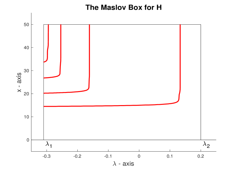
Figure 5.1: The Full Maslov Box for $H$ on $[-.31,.2]$.

5.2 Energy Levels for the Hydrogen Atom

When Schrödinger’s equation for the hydrogen atom is expressed in spherical coordinates and analyzed by separation of variables, the resulting radial equation can be expressed in the form

$$H\phi:=-\frac{1}{x^{2}}(x^{2}\phi^{\prime})^{\prime}-\frac{\gamma}{x}\phi+\frac{\ell(\ell+1)}{x^{2}}\phi=\lambda\phi,$$ (5.5)

where $\gamma>0$ is a physical constant and $\ell$ is an integer associated with angular momentum (see, e.g., Chapter 12 in [16]). The natural domain for (5.5) is $(0,\infty)$, and it’s clear that $H$ is singular at both endpoints. In order to place this equation in our setting, we set $y={y_{1}\choose y_{2}}={\phi\choose x^{2}\phi^{\prime}}$, from which we arrive at (1.1) with

$$B_{0}(x)+\lambda B_{1}(x)=\begin{pmatrix}\gamma x-\ell(\ell+1)&0\\ 0&\frac{1}{x^{2}}\end{pmatrix}+\lambda\begin{pmatrix}x^{2}&0\\ 0&0\end{pmatrix}.$$

It’s well-known that any self-adjoint extension of the minimal operator associated with $H$ has essential spectrum $[0,+\infty)$ (see, e.g., [36]). The eigenvalues of $H$ are typically reported in physics literature to be

$$\lambda_{n}=-(\frac{\gamma}{2n})^{2},\quad n=\ell+1,\ell+2,\dots$$ (5.6)

(see, e.g., [16]), and in this section we would like to understand how this relation should be interpreted in our setting. (See Remark 5.5 below for a formulation of $H$, including its precise domain.) For computational purposes, we’ll take $\gamma=4$, and we’ll focus on the case $\ell=0$, which is particularly interesting from our point of view because $H$ is limit-circle at $x=0$ in this case, whereas it is limit-point at $x=0$ for all $\ell\geq 1$.

We begin by setting $\lambda_{0}=i$ and verifying (numerically) that $H$ is limit-circle at $x=0$. In this case, we initialize the fundamental matrix $\Phi(x;\lambda_{0})$ at $x=1$, and we compute the eigenvalues of $\mathcal{A}(x;\lambda_{0})$, as $x$ tends toward $0$. At $x=10^{-5}$, we find $\mu_{1}(10^{-5};\lambda_{0})=-.7478$ and $\mu_{2}(10^{-5};\lambda_{0})=.3343$, with both values stable as $x$ continues to decrease, suggesting that $H$ is indeed limit-circle at $x=0$. Respectively, we find the associated unit eigenvectors to be

$$v_{1}(10^{-5};\lambda_{0})={.7834\choose-.0001+.6216i},\quad v_{2}(10^{-5};\lambda_{0})={.0001+.6216i\choose.7834},$$

and we take these vectors as approximations for the limit-obtained eigenvectors $v_{1}^{a}(\lambda_{0})$ and $v_{2}^{a}(\lambda_{0})$. As discussed in Section 2, there will be a single Niessen space for this problem, and it will be spanned by two elements that both lie left in $(0,+\infty)$, namely $y_{1}^{a}(x;\lambda_{0})=\Phi(x;\lambda_{0})v_{1}^{a}(\lambda_{0})$ and $y_{2}^{a}(x;\lambda_{0})=\Phi(x;\lambda_{0})v_{2}^{a}(\lambda_{0})$. In order to specify our boundary condition at $x=0$, we also need to compute

$$\rho=\sqrt{-\mu_{1}(\lambda_{0})/\mu_{2}(\lambda_{0})}=1.4956,$$

and select some $\beta\in\mathbb{C}$ with $|\beta|=\rho$. (See the discussion leading into Lemma 2.3.) Given this choice, we will specify our boundary condition via the element

$$U^{a}(x;\lambda_{0})=\Phi(x;\lambda_{0})(v_{1}^{a}(\lambda_{0})+\beta v_{2}^{a}(\lambda_{0})).$$

We emphasize that each choice of $\beta$ from the circle $|\beta|=\rho$ will correspond with a different boundary condition, and so for a different self-adjoint restriction of $H$. In order to fix a specific case, we will take $\beta$ to be the real value $\beta_{1}=1.4956$, where the subscript anticipates that we will later consider an alternative choice.

Next, we fix $\lambda_{1}=-5$, and construct a frame $\mathbf{X}_{a}(x;\lambda_{1})$ satisfying

$$J\mathbf{X}_{a}^{\prime}=(B_{0}(x)+\lambda_{1}B_{1}(x))\mathbf{X}_{a};\quad\lim_{x\to a^{+}}U^{a}(x;\lambda_{0})^{*}J\mathbf{X}_{a}(x;\lambda_{1})=0.$$ (5.7)

In order to do this, we work with the matrix $\mathcal{B}(x;\lambda_{1})$, for which we compute the eigenvalues $\{\nu_{j}(x;\lambda_{1})\}_{j=1}^{2}$ and the associated eigenvectors $\{w_{j}(x;\lambda_{1})\}_{j=1}^{2}$ as $x$ tends to $0$. Taking an approximation obtained by evaluating $\mathcal{B}(x;\lambda_{1})$ at $x=10^{-5}$, we obtain the approximate values $\nu_{1}^{a}(\lambda_{1})=-.4205$, $\nu_{2}^{a}(\lambda_{1})=-.1106$, with associated approximate limit-obtained unit vectors

$$w_{1}^{a}(\lambda_{1})={-.8615\choose.5077},\quad w_{2}^{a}(\lambda_{1})={-.5077\choose-.8615}.$$

We can now compute $\mathbf{X}_{a}(x;\lambda_{1})$ as a linear combination

$$\mathbf{X}_{a}(x;\lambda_{1})=\Phi(x;\lambda_{1})(c_{1}w_{1}^{a}(\lambda_{1})+c_{2}w_{2}^{a}(\lambda_{1})),$$

for some appropriate constants $c_{1}$ and $c_{2}$. In particular, $c_{1}$ and $c_{2}$ are determined by the limit specified in (5.7). We can express this as

$$c_{1}\lim_{x\to a^{+}}U^{a}(x;\lambda_{0})^{*}J\Phi(x;\lambda_{1})w_{1}^{a}(\lambda_{1})+c_{2}\lim_{x\to a^{+}}U^{a}(x;\lambda_{0})^{*}J\Phi(x;\lambda_{1})w_{2}^{a}(\lambda_{1})=0.$$

We approximate the limits by evaluation at $x=10^{-5}$ to obtain

$$\lim_{x\to a^{+}}U^{a}(x;\lambda_{0})^{*}J\Phi(x;\lambda_{1})w_{1}^{a}(\lambda_{1}) \cong-1.2050+1.2050i$$

$$\lim_{x\to a^{+}}U^{a}(x;\lambda_{0})^{*}J\Phi(x;\lambda_{1})w_{2}^{a}(\lambda_{1}) \cong-.6139+.6139i.$$

It follows immediately that we can choose $c_{1}$ and $c_{2}$ to be $c_{1}=1$, $c_{2}=(-1.2050+1.2050i)/(-.6139+.6139i)=-1.9629$. We conclude that

$$\mathbf{X}_{a}(x;\lambda_{1})=\Phi(x;\lambda_{1})w^{a}(\lambda_{1});\quad w^{a}(\lambda_{1})={.0613\choose.9981},$$

where $w^{a}(\lambda_{1})$ has been normalized to have unit length.

We now turn to the right endpoint $b=+\infty$. If we evaluate $\mathcal{A}(x;i)$ at $x=25$, we obtain eigenvalues $\mu_{1}(25;i)=1.9352\times 10^{-22}$ and $\mu_{2}(25;i)=4.6925\times 10^{11}$. This indicates that $\mu_{2}(x;i)$ is tending toward $+\infty$ as $x$ increases to $+\infty$, and we conclude that $H$ is limit-point at $b=+\infty$. This means that no additional boundary condition is necessary at $b=+\infty$. We will denote by $H_{\beta_{1}}$ the operator obtained from $H$ by adding our choice of boundary condition taken above at the left endpoint.

Remark 5.4.

Similarly as with our first application, these calculations have not been rigorously justified, but the limit-circle/point conclusions have been rigorously justified elsewhere. In particular, if we adopt the change of variables $\phi=\psi/x$, then (5.5) with $\ell=0$ becomes

$$\mathcal{H}\psi:=-\psi^{\prime\prime}-\frac{\gamma}{x}\psi=\lambda\psi,$$

which is known to be limit-circle at $x=0$ and limit-point at $+\infty$ (see, e.g., [13]).

In an effort to count the first three eigenvalues of $H$, we will set $\lambda_{2}=-3/8$, and in order to compute $\mathbf{X}_{b}(x;\lambda_{2})$, we will compute the eigenvalues and eigenvectors of $\mathcal{B}(x;\lambda_{2})$ as $x$ tends toward $+\infty$. Taking $x=40$ in this case, we find $\nu_{1}(40;-3/8)=6.3054$ and $\nu_{2}(40;-3/8)=3.7724\times 10^{11}$. The unit eigenvector associated with $\nu_{1}(40;-3/8)$ is

$$w_{1}(40;-3/8)={-.3357895545\choose.9419370335},$$

where similarly as with our previous application, the number of decimals given is simply an indication of the consistent values as $x$ continues to increase. We use $w_{1}(40;-3/8)$ as an approximation of $w_{1}^{b}(-3/8)$, and we set $\mathbf{X}_{b}(x;\lambda_{2})=\Phi(x;\lambda_{2})w_{1}^{b}(-3/8)$.

Equipped now with frames $\mathbf{X}_{a}(x;\lambda_{1})$ and $\mathbf{X}_{b}(x;\lambda_{2})$, we can readily compute

$$\operatorname{Mas}(\ell_{a}(\cdot;\lambda_{1}),\ell_{b}(\cdot;\lambda_{2});(0,+\infty))$$ (5.8)

as a spectral flow for the matrix $\tilde{W}(x;\lambda_{1})$ as specified in (4.19). We find conjugate points at approximately $x=1.95$ and $x=5.00$, after which the value of $\tilde{W}(x;\lambda_{1})$ remains near $-1$, without crossing, as $x$ continues to increase. We conclude that $H_{\beta_{1}}$ has two eigenvalues on the interval $[-5,-3/8]$.

Naively, we might have expected to find three eigenvalues on the interval $[-5,-3/8]$ (namely, $-4$, $-1$, $-4/9$), but we recall that the eigenvalues given in (5.6) correspond with a particular choice of boundary condition (based on physical considerations). In particular, the argument from physics goes roughly as follows. For $\ell=0$, equation (5.5) has two linearly independent solutions, one of which is bounded as $x$ approaches $0$, while the other is unbounded. (Both of which correspond via the above relation $y={y_{1}\choose y_{2}}={\phi\choose x^{2}\phi^{\prime}}$ with functions that lie left in $(0,+\infty)$.) Based on physical arguments, the unbounded solution is generally eliminated, and this effectively selects a particular left-hand boundary condition. Precisely, this physical argument asserts that we need to identify a fixed vector $w\in\mathbb{C}^{2}$ so that $\mathbf{X}_{a}(x;\lambda_{1})=\Phi(x;\lambda_{1})w$ remains bounded as $x$ approaches 0. By a straightforward minimization argument, we find $w={.7121\choose-.7020}$. This solution corresponds with a particular choice of $\beta$. In particular, we can identify the value of $\beta\in\mathbb{C}$, $|\beta|=\rho$ so that

$$\lim_{x\to 0^{+}}\Big{(}\Phi(x;\lambda_{0})(v_{1}(\lambda_{0})+\beta v_{2}(\lambda_{0}))\Big{)}^{*}J\Phi(x;\lambda_{1})w=0.$$

We can approximate $\beta$ by setting $x=10^{-5}$ and computing

$$\beta\cong-\frac{v_{1}(\lambda_{0})^{*}\Phi(x;\lambda_{0})^{*}J\Phi(x;\lambda_{1})w}{v_{2}(\lambda_{0})^{*}\Phi(x;\lambda_{0})^{*}J\Phi(x;\lambda_{1})w}=.2952-1.4663i.$$

Using this choice of $\beta$ leads to a new boundary condition, specified via $U^{a}(x;\lambda_{0})$, and consequently to a new operator $H_{\beta_{2}}$. Computing (5.8) in this case, we count three eigenvalues by virtue of conjugate points at $.68$, $2.00$, and $5.00$.

We conclude with the following remark, addressing some details that have been set aside during the discussion of this application.

Remark 5.5.

It’s natural to view $H$ as an operator on a weighted Hilbert space $L^{2}_{x^{2}}((0,\infty),\mathbb{C})$ with inner product

$$\langle\phi,\psi\rangle_{x^{2}}=\int_{0}^{+\infty}x^{2}\phi(x)\bar{\psi}(x)dx.$$

With this specification, $H$ is self-adjoint on the domain

$$\operatorname{dom}(H) =\Big{\{}\phi\in L^{2}_{x^{2}}((0,\infty),\mathbb{C}):\phi,\phi^{\prime}\in\operatorname{AC}_{\operatorname{loc}}((0,\infty),\mathbb{C}),$$

$$\quad H\phi\in L^{2}_{x^{2}}((0,\infty),\mathbb{C}),\,\lim_{x\to 0^{+}}\Big{(}\Phi(x;\lambda_{0})(v_{1}(\lambda_{0})+\beta v_{2}(\lambda_{0}))\Big{)}^{*}J{\phi(x)\choose x^{2}\phi^{\prime}(x)}=0\Big{\}}.$$

Likewise, the operator $\mathcal{H}$ from Remark 5.4 is self-adjoint on the domain

$$\operatorname{dom}(\mathcal{H}) =\Big{\{}\psi\in L^{2}((0,\infty),\mathbb{C}):\psi,\psi^{\prime}\in\operatorname{AC}_{\operatorname{loc}}((0,\infty),\mathbb{C}),$$

$$\quad\mathcal{H}\psi\in L^{2}((0,\infty),\mathbb{C}),\,\lim_{x\to 0^{+}}\Big{(}\Psi(x;\lambda_{0})(v_{1}(\lambda_{0})+\beta v_{2}(\lambda_{0}))\Big{)}^{*}J{\psi(x)\choose\psi^{\prime}(x)}=0\Big{\}},$$

where $\Psi(x;\lambda)$ is a fundamental matrix associated with $\mathcal{H}$,

$$J\Psi^{\prime}=\mathcal{B}(x;\lambda)\Psi;\quad\Psi(1;\lambda)=\begin{pmatrix}1&0\\ 1&1\end{pmatrix},\quad\mathcal{B}(x;\lambda)=\begin{pmatrix}\frac{\gamma}{x}+\lambda&0\\ 0&1\end{pmatrix}.$$

With these precise specifications, it’s straightforward to verify that $H$ and $\mathcal{L}$ (the latter constructed as in Lemma 1.1) have precisely the same sets of essential spectrum, and also the same sets of discrete eigenvalues. In addition, these spectral sets also agree with their counterparts for $\mathcal{H}$.

Acknowledgments. The authors are grateful to Yuri Latushkin for bringing [18] to their attention, for suggesting that the problem could be approached with the Maslov index, and for several helpful conversations along the way.

References

• [1] L. Aceto, P. Ghelardoni, and M. Marletta, Numerial computation of eigenvalues in spectral gaps of Sturm–Liouville operators, J. Comp. Appl. Math. 189 (2006) 453–470.
• [2] F. V. Atkinson, H. Langer, R. Mennicken, and A.A. Shkalikov, The essential spectrum of some matrix operators, Math. Nachr. 167 (1994) 5 – 20.
• [3] V. I. Arnol’d, Characteristic class entering in quantization conditions, Func. Anal. Appl. 1 (1967) 1 – 14.
• [4] V. I. Arnol’d, The complex Lagrangian Grassmannian, Func. Anal. Appl. 34 (2000) 208–210.
• [5] B. Booss-Bavnbek and C. Zhu, The Maslov index in symplectic Banach spaces, Mem. Amer. Math. Soc. 252 (2018), no. 1201.
• [6] B. Booss-Bavnbek and K. Furutani, The Maslov index: a functional analytical definition and the spectral flow formula, Tokyo J. Math. 21 (1998), 1–34.
• [7] W.-J. Beyn and J. Lorenz, Stability of traveling waves: dichotomies and eigenvalue conditions on finite intervals, Num. Functional Anal. and Optim. 20 (1999) 201–244.
• [8] W.-J. Beyn, Y. Latushkin, and J. Rottmann-Matthes, Finding eigenvalues of holomorphic Fredholm operator pencils using boundary value problems and contour integrals, Integral equations and operator theory 78 (2014) 155–211.
• [9] S. Bögli, Convergence of sequences of linear operators and their spectra, Integral equations and operator theory 88 (2017) 559 – 599.
• [10] R. Bott, On the iteration of closed geodesics and the Sturm intersection theory, Comm. Pure Appl. Math. 9 (1956) 171–206.
• [11] E. A. Coddington and N. Levinson, Theory of ordinary differential equations, TATA McGraw-Hill Publishing Co. LTD 1955.
• [12] S. Cappell, R. Lee and E. Miller, On the Maslov index, Comm. Pure Appl. Math. 47 (1994), 121–186.
• [13] W. N. Everitt, A catalogue of Sturm-Liouville differential equations, in Sturm-Liouville Theory: Past and Present, Birkhäuser Verlag 2005, W. O. Amrein, A. M. Hinz, and D. B. Pearson, Eds.
• [14] D. E. Edmunds and W. D. Evans, Spectral theory and differential operators, Clarendon Press Oxford (1987).
• [15] K. Furutani, Fredholm-Lagrangian-Grassmannian and the Maslov index, Journal of Geometry and Physics 51 (2004) 269 – 331.
• [16] S. Gasiorowicz, Quantum physics, John Wiley & Sons 1974.
• [17] F. Gesztesy, B. Simon, and G. Teschl, Zeros of the Wronskian and renormalized oscillation theory, American J. Math. 118 (1996) 571–594.
• [18] F. Gesztesy and M. Zinchenko, Renormalized oscillation theory for Hamiltonian systems, Adv. Math. 311 (2017) 569–597.
• [19] P. Howard, S. Jung, and B. Kwon, The Maslov index and spectral counts for Hamiltonian systems on [0,1], J. Dynamics and Differential Equations 30 (2018) 1703–1729.
• [20] P. Howard, Y. Latushkin, and A. Sukhtayev, The Maslov index for Lagrangian pairs on $\mathbb{R}^{2n}$, J. Math. Anal. Appl. 451 (2017) 794–821.
• [21] P. Howard and A. Sukhtayev, The Maslov and Morse indices for Schrödinger operators on $[0,1]$, J. Differential Equations 260 (2016) 4499–4559.
• [22] P. Howard and A. Sukhtayev, Renormalized oscillation theory for linear Hamiltonian systems on $[0,1]$ via the Maslov index, arXiv 1808.08264.
• [23] P. Howard and A. Sukhtayev, The Maslov and Morse Indices for Sturm-Liouville Systems on the Half-Line, Discrete and Continuous Dynamical Systems A 40(2) (2020) 983–1012.
• [24] C. K. R. T. Jones, Y. Latushkin, and S. Sukhtaiev, Counting spectrum via the Maslov index for one dimensional $\theta$-periodic Schrödinger operators, Proceedings of the AMS 145 (2017) 363–377.
• [25] T. Kato, Perturbation Theory for Linear Operators, Springer 1980.
• [26] V. Kostrykin and R. Schrader, Kirchhoff’s rule for quantum wires, J. Phys. A: Math. Gen. 32 (1999) 595–630.
• [27] A. M. Krall, Hilbert space, boundary value problems and orthogonal polynomials, Birkhäuser Verlag 2002.
• [28] P. Kuchment, An overview of periodic elliptic operators, Bull. Amer. Math. Soc. 53 (2016) 343–414.
• [29] Y. Latushkin and A. Sukhtayev, The Evans function and the Weyl-Titchmarsh function, Discrete and Continuous Dyn. Sys. Series S 5 (2012) 939 – 970.
• [30] H. D. Niessen, Singuläre S-hermitesche Rand-Eigenwert Probleme, Manuscripta Math. 3 (1970) 35–68.
• [31] H. D. Niessen, Zum verallgemeinerten zweiten Weylschen Satz, Archiv der Math. 22 (1971) 648–656.
• [32] H. D. Niessen, Greensche Matrix and die Formel von Titchmarch-Kodaira für singuläre S-hermitesche Eigenwert Probleme, J. reine arg. Math. 261 (1972) 164–193.
• [33] J. Phillips, Selfadjoint Fredholm operators and spectral flow, Canad. Math. Bull. 39 (1996), 460–467.
• [34] D. B. Pearson, Quantum scattering and spectral theory, Academic Press 1988.
• [35] R. Piziak, P. L. Odell, and R. Hahn, Constructing projections on sums and intersections, Comp. Math. Appl. 37 (1999) 67–74.
• [36] P. A. Rejto, On the essential spectrum of the hydrogen energy and related operators, Pacific J. Math. 19 (1966) 109–140.
• [37] J. Robbin and D. Salamon, The Maslov index for paths, Topology 32 (1993) 827 – 844.
• [38] M. Reed and B. Simon, Methods of modern mathematical physics IV: Analysis of operators, Academic Press 1978.
• [39] H. Schulz-Baldes, Rotation numbers for Jacobi matrices with matrix entries, Math. Phys. Electron. J. 13 (2007), Paper 5, 40 pp.
• [40] H. Schulz-Baldes, Sturm intersection theory for periodic Jacobi matrices and linear Hamiltonian systems, Linear Algebra Appl. 436 (2012), no. 3, 498–-515.
• [41] B. Simon, Sturm oscillation and comparison theorems, in Sturm-Liouville Theory: Past and Present, Birkhäuser Verlag 2005, W. O. Amrein, A. M. Hinz, and D. B. Pearson, Eds.
• [42] C. Sturm, Mémoire sur les équations différentielles linéaires du second ordre, J. math. pures appl. 1 (1836) 106–186.
• [43] G. Teschl, Oscillation theory and renormalized oscillation theory for Jacobi operators, J. Differential Equations 129 (1996) 532–558.
• [44] G. Teschl, Renormalized oscillation theory for Dirac operators, Proceedings of the AMS 126 (1998) 1685–1695.
• [45] J. Weidmann, Linear Operators in Hilbert spaces, Springer–Verlag 1980.
• [46] J. Weidmann, Spectral theory of ordinary differential operators, Springer-Verlag 1987.
• [47] J. Weidmann, Strong operator convergence and spectral theory of ordinary differential operators, Universitatis Iagellonicae acta Mathematica, Fasciculus XXXIV (1997) 153–163.