Accelerated Gradient Methods for Sparse Statistical Learning with Nonconvex Penalties

Abstract

Nesterov’s accelerated gradient (AG) is a popular technique to optimize objective functions comprising two components: a convex loss and a penalty function. While AG methods perform well for convex penalties, such as the LASSO, convergence issues may arise when it is applied to nonconvex penalties, such as SCAD. A recent proposal generalizes Nesterov’s AG method to the nonconvex setting. The proposed algorithm requires specification of several hyperparameters for its practical application. Aside from some general conditions, there is no explicit rule for selecting the hyperparameters, and how different selection can affect convergence of the algorithm. In this article, we propose a hyperparameter setting based on the complexity upper bound to accelerate convergence, and consider the application of this nonconvex AG algorithm to high-dimensional linear and logistic sparse learning problems. We further establish the rate of convergence and present a simple and useful bound to characterize our proposed optimal damping sequence. Simulation studies show that convergence can be made, on average, considerably faster than that of the conventional proximal gradient algorithm. Our experiments also show that the proposed method generally outperforms the current state-of-the-art methods in terms of signal recovery.

Keywords: Optimization, Statistical Computing, Variable Selection

1 Introduction

Sparse learning is an important component of modern data science and is an essential tool for the statistical analysis of high-dimensional data, with significant applications in signal processing and statistical genetics, among others. Penalization is commonly used to achieve sparsity in parameter estimation. The prototypical optimization problem for obtaining penalized estimators is

$$\hat{\bm{\beta}}\in\arg\min_{\bm{\beta}\in\mathbb{R}^{q+1}}\left[f\left(\bm{\beta}\right)+\sum_{j=1}^{q}p_{\lambda}\left(\beta_{j}\right)\right],$$

where $f\mathrel{\mathop{\mathchar 58\relax}}\mathbb{R}^{q+1}\mapsto\mathbb{R}$ is a convex loss function, $p_{\lambda}\mathrel{\mathop{\mathchar 58\relax}}\mathbb{R}\mapsto\mathbb{R}_{\geq 0}$ constitutes the penalty term, and $\lambda>0$ is the tuning parameter for the penalty. Commonly used penalization methods for sparse learning include: LASSO (Least Absolute Shrinkage and Selection Operator) [1], Elastic Net [2], SCAD (Smoothly Clipped Absolute Deviation) [3] and MCP (Minimax Concave Penalty) [4]. Among these penalties, parameter estimation with SCAD and MCP leads to a nonconvex objective function. The nonconvexity poses a challenge in statistical computing, as most methods developed for convex objective functions might not converge when applied to the nonconvex counterpart.

Various approaches have been proposed to carry out parameter estimation with SCAD or MCP penalties. [5] [*]Zou2008 proposed a local linear approximation, which yields a first-order majorization-minimization (MM) algorithm. [6] [*]Kim2008 discussed a difference-of-convex programming (DCP) method for ordinary least square estimators penalized by the SCAD penalty, which was later generalized by [7] [*]Wang2013 to a general class of nonconvex penalties to produce a first-order algorithm. These first-order methods belong to the class of proximal gradient descent methods, which are usually inefficient as relaxation is often expensive [8]. The objective function is often ill-conditioned for sparse learning problems, and gradient descent with constant step size is especially inefficient for high-dimensional problems. Indeed, previous studies have suggested that the condition number of a square random matrix grows linearly with respect to its dimension [9]. Therefore, high-dimensional problems have a large condition number with high probability. Specific to gradient descent with constant step size, the trajectory will oscillate in the directions with a large eigenvalue, moving very slowly toward the directions with a small eigenvalue, making the algorithm inefficient. [10] [*]Lee2016 developed a modified second-order method originally designed for the ordinary least square loss function penalized by LASSO with extensions to SCAD and MCP; this attempt was later extended to generalized linear models, such as logistic and Poisson regression, and Cox’s proportional hazard model. Quasi-Newton methods, or a mixture of first and second-order descent methods, have also been applied on nonconvex penalties [11, 12]. However, for high-dimensional problems, these second-order methods are slow due to the computational cost of evaluating the secant condition. Concurrently, most first and second-order methods discussed above require a line-search procedure at each step to ensure global convergence, which is prohibitive when the number of parameters to estimate grows large. [13] [*]Breheny2011 implemented a coordinate descent method in the ncvreg R package to carry out estimation for linear models with least squares loss or logistic regression, penalized by SCAD and MCP. [14] [*]Mazumder2011 also implemented a coordinate descent method in the sparsenet R package, which carries out a closed-form root-finding update in a coordinate-wise manner for penalized linear regression. Similar to how ill-conditioning makes gradient descent inefficient, coordinate descent methods are generally inefficient when the covariate correlations are high [15]. Previous studies have also found that coordinate-wise minimization might not converge for some nonsmooth objective functions [16]. Furthermore, it is naturally challenging to run coordinate-wise minimization in parallel, as the algorithm must run in a sequential coordinate manner.

Due to the low computational cost and adequate memory requirement per iteration, first-order methods without a line search procedure have become the primary approach for high-dimensional problems arising from various areas [17]. For smooth convex objective functions, Nesterov proposed the accelerated gradient method (AG) to improve the rate of convergence from $O(1/N)$ for gradient descent to $O(1/N^{2})$ while achieving global convergence [18]. Subsequently, Nesterov extended AG to composite convex problems [19], whereas the objective is the sum of a smooth convex function and a simple nonsmooth convex function. With proper step-size choices, Nesterov’s AG was later shown optimal to solve both smooth and nonsmooth convex programming problems [20].

Given that sparse learning problems are often high-dimensional, Nesterov’s AG has been frequently used for convex problems in statistical machine learning (e.g., [21, 22, 23, 24]). However, convergence is questionable if the convexity assumption is violated. Recently, [25] [*]Ghadimi2015 generalized the AG method to nonconvex objective functions, hereafter referred to as the nonconvex AG method, and derived the rates of convergence for both smooth and composite objective functions. While this method can be applied to nonconvex sparse learning problems, several hyperparameters must be set prior to running the algorithm and can be difficult to choose in practice. Indeed, the nonconvex AG method has never been applied in the context of sparse statistical learning problems with nonconvex penalties, such as SCAD and MCP.

This manuscript presents a detailed analysis of the complexity upper bound of the nonconvex AG algorithm and proposes a hyperparameter setting to accelerate convergence (Theorem 1). We further establish the rate of convergence (Theorem 2) and present a simple and useful bound to characterize our proposed optimal damping sequence (Theorem 3 and Corollary 1). Our simulation studies on penalized linear and logistic models show that the nonconvex AG method with the proposed hyperparameter selector converges considerably faster than other first-order methods. We also compare the signal recovery performance of the algorithm to that of ncvreg, the state-of-the-art method based on coordinate descent, showing that the proposed method outperforms the state-of-the-art coordinate descent method.

The rest of this manuscript is organised as follows. In Sections 2, 3, 4, we will present an analysis of the nonconvex AG algorithm by [25] to illustrate the algorithm as a generalization of Nesterov’s AG. We also present formal results about the effect of hyperparameter settings on the complexity upper bound. Section 5 will include simulation studies for linear and logistic models penalized by SCAD and MCP penalties. The simulation studies show that i) The AG method using our proposed hyperparameter settings converges faster than commonly used first-order methods for data with various $q/n$ and covariate correlation settings; and ii) our method outperforms the current state-of-the-art method, i.e. ncvreg, in terms of signal recovery performance, especially when the signal-to-noise ratios are low. The proofs for the theorems are included in the Appendix A.

2 Motivation and Setup

Having built on Nesterov’s seminal work, [25] [*]Ghadimi2015 considered the following composite optimization problem:

$$\min_{x\in\mathbb{R}^{q+1}}\Psi\left(x\right)+\chi\left(x\right),\ \Psi\left(x\right)\coloneqq f\left(x\right)+h\left(x\right), \mathcal{P}$$ ()

where $f\in\mathcal{C}_{L_{f}}^{1,1}(\mathbb{R}^{q+1},\mathbb{R})$ is convex, $h\in\mathcal{C}_{L_{h}}^{1,1}(\mathbb{R}^{q+1},\mathbb{R})$ is possibly nonconvex, and $\chi$ is a convex function over a bounded domain, and $\mathcal{C}_{L}^{1,1}$ denotes the class of first-order Lipschitz smooth functions with $L$ being the Lipschitz constant. They devised Algorithm 1 discussed in details in next section, and presented a theoretical analysis of their algorithm.

Some commonly used nonconvex penalties, such as SCAD and MCP, have a form that can naturally be decomposed into summation of a convex and a nonconvex function satisfying the conditions required by [25] [*]Ghadimi2015. When such penalties are added to a smooth convex deviance measure, such as negative of typical log-likelihoods, the resulting optimization problem follows the form of optimization problem $\mathcal{P}$. As we show below this is, in particular, the case when the deviance measure is a quadratic loss and the penalty is either SCAD or MCP. The quadratic loss plays the role of $f$. The other two functions, i.e. $h$ and $\chi$ are specified for both SCAD and MCP penalties. Define

$$p_{\lambda,a,\text{SCAD}}\left(\bm{\beta}\right)=\chi\left(\bm{\beta}\right)+h_{\text{SCAD}}\left(\bm{\beta}\right),$$ (1)

$$p_{\lambda,\gamma,\text{MCP}}\left(\bm{\beta}\right)=\chi\left(\bm{\beta}\right)+h_{\text{MCP}}\left(\bm{\beta}\right);$$ (2)

where $\bm{\beta}\coloneqq\left[\beta_{0},\beta_{1},\dots,\beta_{q}\right]^{T}$, $\chi\left(\bm{\beta}\right)=\sum_{j=1}^{q}\lambda\lvert\beta_{j}\rvert$, and

$$h_{\text{SCAD}}\left(\bm{\beta}\right)=\sum_{j=1}^{q}\begin{cases}0;&\lvert\beta_{j}\rvert\leq\lambda\\ \frac{2\lambda\lvert\beta_{j}\rvert-\beta_{j}^{2}-\lambda^{2}}{2\left(a-1\right)};&\lambda<\lvert\beta_{j}\rvert<a\lambda\\ \frac{1}{2}\left(a+1\right)\lambda^{2}-\lambda\lvert\beta_{j}\rvert;&\lvert\beta_{j}\rvert\geq a\lambda\end{cases} \in\mathcal{C}_{L_{\text{SCAD}}}^{1,1}$$ (3)

$$h_{\text{MCP}}\left(\bm{\beta}\right)=\sum_{j=1}^{q}\begin{cases}-\frac{\beta_{j}^{2}}{2\gamma};&\lvert\beta_{j}\rvert<\gamma\lambda\\ \frac{1}{2}\gamma\lambda^{2}-\lambda\lvert\beta_{j}\rvert;&\lvert\beta_{j}\rvert\geq\gamma\lambda\end{cases} \in\mathcal{C}_{L_{\text{MCP}}}^{1,1}$$ (4)

In the above equations, $\lambda>0,a>2,\gamma>1$ are the penalty tuning parameters. It is trivial that, in (1) and (2), $\chi\left(\bm{\beta}\right)$ is convex and the remaining term is a first-order smooth concave function. In view of the optimization problem $\mathcal{P}$, when applying SCAD/MCP on a convex $\mathcal{C}_{L_{\ell}}^{1,1}$ statistical learning objective function, $f=-2\ell$ will be the convex component; $h_{\text{SCAD}},h_{\text{MCP}}$ will be the smooth nonconvex component with $L_{SCAD}=\frac{1}{a-1}$ and $L_{MCP}=\frac{1}{\gamma}$; and $\chi=\sum_{j=1}^{q}\lambda\lvert\beta_{j}\rvert$ will be the nonsmooth convex component. For high-dimensional statistical learning problems, the L-smoothness constant for the smooth nonconvex component, $L_{SCAD}$ and $L_{MCP}$, are often negligible when compared to the greatest singular value of the design matrix [26]. In statistical learning applications, most unconstrained problems can, in fact, be reduced to problems over a bounded domain, as information often suggests the boundedness of the variables.

3 The Accelerated Gradient Algorithm

This Section comprises two subsections. Subsection 3.1 includes an algorithm proposed by [25] [*]Ghadimi2015 for solving the composite optimization problem $\mathcal{P}$. In Subsection 3.2 we propose an approach for selecting the hyperparameters of the algorithm by minimizing the complexity upper bound (10)

3.1 Nonconvex Accelerated Gradient Method

Building on Nesterov’s AG algorithm, [25] [*]Ghadimi2015 proposed the following algorithm for solving the composite optimization problem $\mathcal{P}$.

Algorithm 1 Accelerated Gradient Algorithm

0:  starting point $x_{0}\in\mathbb{R}^{q+1}$, $\{\alpha_{k}\}$ s.t. $\alpha_{1}=1$ and $\forall k\geq 2,0<\alpha_{k}<1$, $\{\omega_{k}>0\}$, and $\{\delta_{k}>0\}$

  0. Set $x_{0}^{ag}=x_{0}$ and $k=1$

  1. Set

$$x_{k}^{md}=\alpha_{k}x_{k-1}^{ag}+\left(1-\alpha_{k}\right)x_{k-1}$$ (5)

  2. Compute $\nabla\Psi\left(x_{k}^{md}\right)$ and set

$$x_{k}= x_{k-1}-\delta_{k}\nabla\Psi\left(x_{k}^{md}\right)\text{ (smooth)} x_{k}= \mathcal{P}\left(x_{k-1},\nabla\Psi\left(x_{k}^{md}\right),\delta_{k}\right)\text{ (composite)}$$ (6)

$$x_{k}^{ag}= x_{k}^{md}-\omega_{k}\nabla\Psi\left(x_{k}^{md}\right)\text{ (smooth)} x_{k}^{ag}= \mathcal{P}\left(x_{k}^{md},\nabla\Psi\left(x_{k}^{md}\right),\omega_{k}\right)\text{ (composite)}$$ (7)

  3. Set $k=k+1$ and go to step 1

  Minimizer $x_{N}^{md}$

In Algorithm 1, “smooth” represents the updating formulas for smooth problems, and “composite” represents the update formulas for composite problems, and $\mathcal{P}$ is the proximal operator defined as:

$$\mathcal{P}\left(x,y,c\right)\coloneqq\arg\min_{u\in\mathbb{R}^{q+1}}\left\{\left\langle y,u\right\rangle+\frac{1}{2c}\left\|u-x\right\|^{2}+\chi\left(u\right)\right\}.$$

It is evident that the composite counter-part of the algorithm is the Moreau envelope smoothing of the simple nonconvex function; for this reason, in later analysis of the algorithm, we will use smooth updating formulas for the sake of parsimony. As an interpretation of the algorithm, $\left\{\alpha_{k}\right\}$ controls the damping of the system, and $\omega_{k}$ controls the step size for the “gradient correction” update for momentum method. In what follows, $\Gamma_{k}$ is defined recursively as:

$$\Gamma_{k}\coloneqq\begin{cases}1,&k=1;\\ \left(1-\alpha_{k}\right)\Gamma_{k-1},&k\geq 2.\end{cases}$$

[25] [*]Ghadimi2015 proved that under the following conditions:

$$\alpha_{k}\delta_{k}\leq\omega_{k}<\frac{1}{L_{\Psi}},\ \forall k=1,2,\dots N-1\text{ and}$$ (8)

$$\frac{\alpha_{1}}{\delta_{1}\Gamma_{1}}\geq\frac{\alpha_{2}}{\delta_{2}\Gamma_{2}}\geq\cdots\geq\frac{\alpha_{N}}{\delta_{N}\Gamma_{N}},$$ (9)

the rate of convergence for composite optimization problems can be illustrated by the following complexity upper bound:

$$\min_{k=1,\dots,N}\left\|\mathcal{G}\left(x_{k}^{md},\nabla\Psi\left(x_{k}^{md}\right),\omega_{k}\right)\right\|^{2}$$

$$\hskip 86.72377pt\leq\left[\sum_{k=1}^{N}\Gamma_{k}^{-1}\omega_{k}\left(1-L_{\Psi}\omega_{k}\right)\right]^{-1}\left[\frac{\left\|x_{0}-x^{*}\right\|^{2}}{\delta_{1}}+\frac{2L_{h}}{\Gamma_{N}}\left(\left\|x^{*}\right\|^{2}+M^{2}\right)\right].$$ (10)

In the above inequality, $\mathcal{G}\left(x_{k}^{md},\nabla\Psi\left(x_{k}^{md}\right),\omega_{k}\right)$ is the analogue to the gradient for smooth functions defined by:

$$\mathcal{G}\left(x,y,c\right)\coloneqq\frac{1}{c}\left[x-\mathcal{P}\left(x,y,c\right)\right].$$

In accelerated gradient settings, $x$ corresponds to the past iteration, $y$ corresponds to the smooth gradient at $x$, and $c$ corresponds to the step size taken.

3.2 Hyperparameters for Nonconvex Accelerated Gradient Method

Here we discuss how hyperparameters, $\alpha_{k}$, $\omega_{k}$ and $\delta_{k}$ can be selected to accelerate convergence of Algorithm 1 by minimizing the complexity upper bound. From Lemma 1, it is clear that the conditions (8) and (9) merely present a lower bound for the vanishing rate of $\left\{\alpha_{k}\right\}$. We also observe that the right-hand side of (19) is monotonically increasing with respect to $\alpha_{k}$; thus, to obtain the maximum values for $\left\{\alpha_{k}\right\}$, it is sufficient to maximize $\alpha_{k}$ recursively.

Using (5), (6), and (7), we have

$$\frac{x_{k+1}^{md}-\left(1-\alpha_{k+1}\right)x_{k}^{ag}}{\alpha_{k+1}}= \frac{x_{k}^{md}-\left(1-\alpha_{k}\right)x_{k-1}^{ag}}{\alpha_{k}}-\delta_{k}\nabla\Psi\left(x_{k}^{md}\right)\text{ and}$$

$$x_{k}^{ag}= x_{k}^{md}-\omega_{k}\nabla\Psi\left(x_{k}^{md}\right).$$

By sorting out the terms in the above equations, we obtain the following updating formulas:

$$x_{k}^{ag}= x_{k}^{md}-\omega_{k}\nabla\Psi\left(x_{k}^{md}\right)$$ (11)

$$x_{k+1}^{md}= x_{k}^{ag}+\alpha_{k+1}\cdot\left(\frac{1}{\alpha_{k}}-\frac{\delta_{k}}{\omega_{k}}\right)\cdot\left(\omega_{k}\nabla\Psi\left(x_{k}^{md}\right)\right)+\alpha_{k+1}\cdot\left(\frac{1}{\alpha_{k}}-1\right)\left(x_{k}^{ag}-x_{k-1}^{ag}\right)$$ (12)

Compared to Nesterov’s AG, the AG method proposed by Ghadimi and Lan differs by the convergence conditions (8) and (9), and the inclusion of the term $\alpha_{k+1}\cdot\left(\frac{1}{\alpha_{k}}-\frac{\delta_{k}}{\omega_{k}}\right)\cdot\left(\omega_{k}\nabla\Psi\left(x_{k}^{md}\right)\right)$ in (12). Since $\alpha_{k+1}\cdot\left(\frac{1}{\alpha_{k}}-\frac{\delta_{k}}{\omega_{k}}\right)\geq 0$ is implied by convergence condition (8), this added term functions as a step to reduce the magnitude of “gradient correction” presented in (11): the resulting framework will keep the same momentum compared to Nesterov’s AG, but the momentum step update will occur at a midpoint between $x_{k}^{ag}$ and $x_{k}^{md}$ to yield $x_{k+1}^{md}$. Such a framework suggests that the proposed algorithm is merely a midpoint generalization in the gradient correction step of Nesterov’s AG. Therefore, the acceleration occurs to the convex component $f$ of the objective function $\Psi$. Following this intuition, we proceed to investigate the optimization hyperparameter settings for the most accelerating effect in Theorem 1 based on the idea of minimizing the complexity upper bound (10) when the objective function is convex; i.e., when $h\equiv 0$.

It can be deduced from (19) that an increasing sequence of $\left\{\delta_{k}\right\}$ allows a slower vanishing rate for $\left\{\alpha_{k}\right\}$. Specifically, the existence of $\delta_{1}$ in (10) can be explained as the following: the momentum initialization step in Algorithm 1 indicates that $x_{1}^{md}=x_{0}^{ag}=x_{0}$. We also have $x_{1}^{ag}=x_{1}^{md}-\omega_{1}\nabla\Psi\left(x_{1}^{md}\right)=x_{0}^{ag}-\omega_{1}\nabla\Psi\left(x_{0}\right)$ for smooth problems or $x_{1}^{ag}=\mathcal{P}\left(x_{1}^{md},\nabla\Psi\left(x_{1}^{md}\right),\omega_{1}\right)=\mathcal{P}\left(x_{0}^{ag},\nabla\Psi\left(x_{0}\right),\omega_{1}\right)$ for composite problems. In view of (12), the momentum initializes as $x_{1}^{ag}-x_{0}^{ag}=-\omega_{1}\nabla\Psi\left(x_{0}\right)$ for smooth problems. Thus, should $\delta_{1}<\omega_{1}$ take a smaller value, $\alpha_{2}\cdot\left(\frac{1}{\alpha_{1}}-\frac{\delta_{1}}{\omega_{1}}\right)>0$; i.e., $x_{2}^{md}$ is a convex combination of $x_{1}^{ag}$ and the initial point $x_{0}$, and the smaller $\delta_{1}$ is, the closer $x_{2}^{md}$ is to $x_{0}$. Meanwhile, a smaller $\delta_{1}$ allows a faster increasing sequence $\left\{\delta_{k}\right\}$; hence a slower-vanishing sequence $\left\{\alpha_{k}\right\}$ can be achieved to incorporate more momentum. This process can be interpreted as follows: when $x_{2}^{md}$ does not retain the full step update from the initial point $x_{0}$, more initial momentum will be allowed to accumulate, as the initial momentum is in the same direction as the update. We therefore choose $\delta_{1}=\omega_{1}$; i.e., to let $x_{2}^{md}$ retain fully the update from $x_{0}$ in the direction of $-\omega_{1}\nabla\Psi\left(x_{0}\right)$, such that no excess initial momentum will be needed to account for initial update deficiency in this direction.

4 Theoretical Analysis of the Algorithm

For gradient methods without a line-search procedure, the step size for the gradient correction is usually set to be a constant. Based on this convention, we assume $\omega_{k}=\beta$ for $k=1,2,\dots,N$. Theorem 1 below presents the optimal choice of hyperparameters under mild conditions.

Theorem 1.

Assume conditions (8) and (9) hold. Let $\delta_{1}=\omega_{k}=\omega$ and $h=0$. Then the complexity upper bound (10) is minimized by:

$$\bar{\alpha}_{k+1}= \frac{2}{1+\sqrt{1+\frac{4}{\bar{\alpha}_{k}^{2}}}},\ \bar{\alpha}_{1}=1,$$ (13)

$$\bar{\delta}_{k+1}= \frac{\bar{\omega}}{\bar{\alpha}_{k+1}},$$ (14)

$$\bar{\omega}= \frac{2}{3L_{\Psi}}.$$ (15)

Proof.

See Appendix A.1. ∎

As illustrated by the proof of the above theorem, the optimization hyperparameter settings (13), (14), and (15) allow for the greatest values of $\left\{\alpha_{k}\right\}$ under the constant gradient-correction step size and maximum initial update assumptions; i.e., condition 1. Such settings allow the most acceleration for the convex component. Although a greater momentum will result in a much faster convergence at the initial stage of the algorithm, it will also result in oscillations of larger magnitudes near the minimizer. Therefore, in the following theorem, we will show that the complexity upper bound will always maintain $O\left(1/N\right)$ rate of convergence. This observation implies that the accelerated gradient method’s worst-case scenario is at least as good as $O\left(1/N\right)$ for gradient descent in terms of the rate of convergence.

Theorem 2.

Assume conditions (8) and (9) hold. Then under the assumptions of Theorem 1, the complexity upper bound is $O\left(1/N\right)$.

Proof.

See Appendix A.2. ∎

The recursive formula for optimal momentum hyperparameter, $\left\{\alpha_{k}\right\}$, as presented in (13), is of a rather complicated structure. The next theorem illustrates the vanishing rate of $\left\{\alpha_{k}\right\}$.

Theorem 3.

Let $\bar{\alpha}_{1}=1$ and (13) holds. Then

$$\frac{2}{\left(1+a\cdot k^{-b}\right)k+1}<\bar{\alpha}_{k}\leq\frac{2}{k+1},\quad k=1,\dots,N,$$ (16)

for any $a>0,\ 0<b<1$, such that

$$a\left(1-b\right)\cdot 2^{2-b}-ab\left(1-b\right)\cdot 2^{-b}-1\geq 0.$$ (17)

Proof.

See Appendix A.3. ∎

The following corollary establishes a tight bound for the damping sequence, hence providing the speed of convergence of our proposed optimal damping sequence $\left\{\bar{\alpha}_{k}\right\}$ to $\frac{2}{k+1}$.

Corollary 1.

The lower bound in (16) is maximized at

$$\bar{a}_{k}=\frac{2^{\bar{b}_{k}}}{\left(1-\bar{b}_{k}\right)\left(4-\bar{b}_{k}\right)}\quad\text{and}\quad\bar{b}_{k}=\frac{2+5\left(\log\frac{2}{k}\right)+\sqrt{9\left(\log\frac{2}{k}\right)^{2}+4}}{2\left(\log\frac{2}{k}\right)}\quad\text{for}\quad k\geq 8.$$

The lower bound in (16) therefore becomes

$$\frac{k+1}{2}-\bar{\alpha}_{k}^{-1}=O\left(\log k\right)$$ (18)

Proof.

See Appendix A.4. ∎

To better illustrate Corollary 1, we plot the value of $\log\left(\bar{a}_{k}k^{-b}\right)$ v.s. $(k,b)$ in Figure 1. The plot shows that as $k$ grows large, the optimizer $\bar{b}_{k}$ converges to $1$ at a very slow rate. It also reflects on the speed of $1+\bar{a}_{k}\cdot k^{-\bar{b}_{k}}$, the coefficient of $k$ in the denominator of the lower bound in (16), goes to $1$ as $k$ increases.

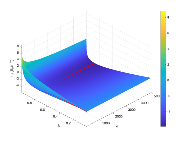
Figure 1: Numerical plots for Corollary 1. The figure plots $\log\left(\bar{a}_{k}k^{-b}\right)$ v.s. $k$ and $b$; the red line plots its minimizer $\bar{b}_{k}=\frac{2+5\left(\log\frac{2}{k}\right)+\sqrt{9\left(\log\frac{2}{k}\right)^{2}+4}}{2\left(\log\frac{2}{k}\right)}$ for each $k$. The plot reflects on the speed for the coefficient of $k$ in the denominator of the lower bound in (16) converges to $1$. The red line shows that $\bar{b}_{k}$ converges to $1$ at an extremely slow rate.

5 Simulations Studies

In this section, we conduct two sets of simulation studies for nonconvex penalized linear and logistic models. We first visualize the convergence rates and signal recovery performance for each set of simulation studies using a single simulation replicate. Second, we compare the convergence rates across the first-order methods with varying $q/n$ ratios and covariate correlations for $100$ simulation replications. Lastly, we compare the signal recovery performance using our method to the state-of-the-art method, ncvreg [13], with varying covariate correlations and signal-to-noise ratios (SNRs) for $100$ simulation replications. Since the iterative complexity differs for the first-order methods and coordinate descent methods, the convergence rates in terms of the number of iterations are not directly comparable. Thus, we choose to compare the computing time between AG, proximal gradient descent, and coordinate descent.

5.1 Simulation Setup

Linear models with the OLS loss function is a popular method for modelling a continuous response. We aim to achieve signal recovery by solving the following problem for penalized linear models:

$$\arg\min_{\bm{\beta}\in\mathbb{R}^{q+1}}\frac{1}{2n}\left\|\mathbf{X}\bm{\beta}-\mathbf{y}\right\|_{2}^{2}+\sum_{j=1}^{q}p_{\lambda}\left(\beta_{j}\right),$$

where $p_{\lambda}\mathrel{\mathop{\mathchar 58\relax}}\mathbb{R}\mapsto\mathbb{R}_{\geq 0}$ is the SCAD or MCP penalty function. To compare the convergence rates across the first-order methods, we choose different $q/n$ ratios and the strength of correlation, $\tau$, between the covariates. These two parameters are most likely to impact the convergence rates. Median and corresponding $95\%$ bootstrap confidence intervals from $1000$ bootstrap replications for the number of iterations required for the iterative objective values to make a fixed amount of descent are reported. To compare the signal recovery performance between our AG method and the state-of-the-art package ncvreg, we performed $100$ simulation replications with varying SNRs and covariate correlations, as they directly impact the signal recovery performance. The simulation studies we performed adapt the following setups:

• The total number of observations $n=1000$ for visualization plots and signal recovery performance comparison, and $n=200,500,1000,3000$ for convergence rate and computing time comparisons.

• For visualization purposes, we perform one simulation replicate with the number of covariates $q=2004$, with $4$ nonzero signals being $2,-2,8,-8$. We perform $100$ simulation replications with the number of covariates $q=2050$, with $5$ blocks of “true” signals equal-spaced with $500$ zeros in-between for convergence rate and computing time comparison, as well as signal recovery performance comparison. For each simulation replicate, the blocks of the “true” signals are simulated from $N_{10}\left(0.5,1\right)$, $N_{10}\left(5,2\right)$, $N_{10}\left(10,3\right)$, $N_{10}\left(20,4\right)$, $N_{10}\left(50,5\right)$, respectively.

• The design matrix, $\mathbf{X}$, is simulated from a multivariate Gaussian distribution with mean $0$. The covariance matrix $\bm{\Sigma}$ is a $\tau-$Toeplitz matrix, where $\tau=0.5$ for the visualization plots and $\tau=0.1,0.5,0.9$ for the convergence rate and computing time comparison, as well as signal recovery performance comparison. All covariates are standardized; i.e., centered by the sample mean and scaled by the sample standard deviation.

• The signal-to-noise ratio is set as $\text{SNR}=\frac{\sqrt{\bm{\beta}_{\text{true}}^{T}\bm{\Sigma}\bm{\beta}_{\text{true}}}}{\sigma}$, where $\bm{\beta}_{\text{true}}$ are the “true” coefficient values, and $\sigma$ is used as the residual standard deviation. $\text{SNR}=5$ for visualization plots, $\text{SNR}=3$ for convergence rate comparison, and $\text{SNR}=1,3,7,10$ for signal recovery performance comparison.

• For visualization plots, convergence rate and computing time comparisons, we take $\lambda=0.5,a=3.7$ for SCAD and $\lambda=0.5,\gamma=3$ for MCP, unless otherwise specified. For signal recovery rate comparison, $\lambda$ sequence consists of $50$ values equal-spaced from $\lambda_{\max}$ to $0$. The tuning parameter $\lambda$ is chosen to minimize the (non-penalized) loss function value on a validation set of the same size as the training set.

• For signal recovery performance comparison, we use the same objective function as ncvreg to ensure that the same value of penalty tuning parameters results in the same degree of penalization. We also adapt the same strong rule setup as ncvreg [27].

To compare the gradient-based methods and the coordinate descent method, we compare the computing time when both coded in Python/CuPy. The coordinate descent method was coded based on the state-of-the-art pseudo-code [13]. All of the computing was carried out on a NVIDIA A100 GPU with CUDA compute capability of 8.0 on the Narval computing cluster from Calcul Quèbec/Compute Canada. Furthermore, we also excluded the computation of the L-smoothness parameter for the coordinate descent method in our simulations.

The simulation setups for penalized logistic models are similar to those above for penalized linear models, except that the active coefficients are set differently to account for the exponential scale inherent to the logistic regression. For the single-replicate visualization simulations, we let the $4$ nonzero signals be $0.5,-0.5,0.8,-0.8$. For the simulations with $100$ replications to compare the convergence rate and signal recovery performance, we simulate the $5$ blocks of the “true” signals from $N_{10}\left(0.5,1\right)$, $N_{10}\left(0.5,1\right)$, $N_{10}\left(-0.5,1\right)$, $N_{10}\left(-0.5,1\right)$, $N_{10}\left(1,1\right)$, respectively. The SNR for logistic regression has the same definition as linear models, with Gaussian noise added to the generated continuous predictor $\mathbf{X}\bm{\beta}_{true}$. The binary outcomes are independent Bernoulli realizations, with probabilities being the logistic transforms of the continuous response.

5.2 Simulation Results

5.2.1 Penalized Linear Regression

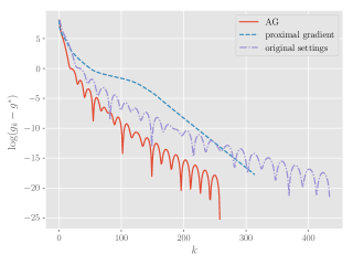
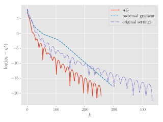
Figure 2: Convergence rate performance of first-order methods on SCAD (left) and MCP (right) penalized linear model for a single simulation replicate. $k$ represents the number of iterations, $g_{k}$ represents the iterative objective function value, and $g^{*}$ represents the minimum found by the three methods considered.

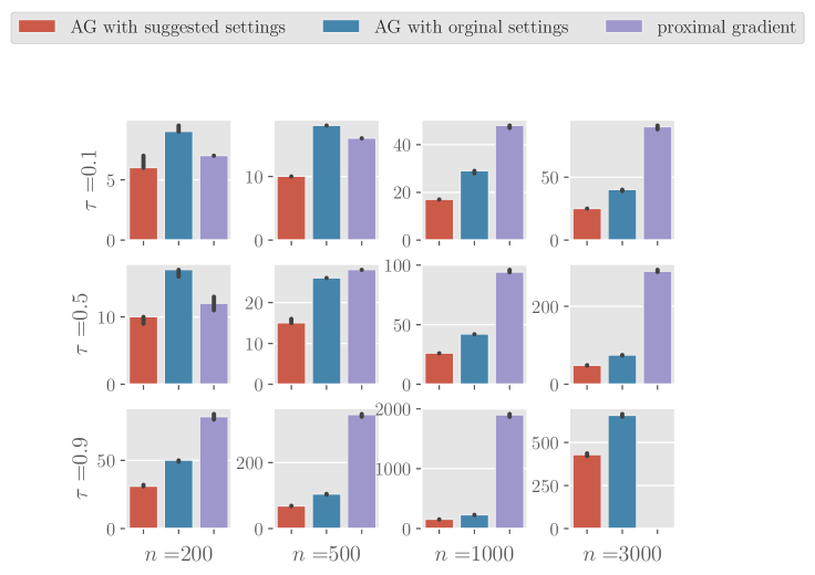
Figure 9: Median for the number of iterations required for iterative objective values to reach $g^{*}+e^{3}$ on MCP-penalized linear model for AG with our proposed hyperparameter settings, AG with original settings, and proximal gradient over $100$ simulation replications, across varying covariates correlation ($\tau$) and $q/n$ values. The error bars represent the $95\%$ CIs from $1000$ bootstrap replications, $g^{*}$ represents the minimum per iterate found by the three methods considered.

Figure 2 shows the log differences of iterative objective values for a single replicate. This figure visualizes the accelerating effect of the AG method using our proposed hyperparameter settings. Median with the corresponding $95\%$ bootstrap CI of the number of iterations required for the iterative objective function values to make a fixed amount of descent for $100$ simulation replications are reported in Figures 8, 9 in Appendix B.1. The lack of bars in the reported barplots indicates that the median of $100$ replications breaks down; i.e., the corresponding proximal gradient algorithm fails to converge to the minimizer found by the three algorithms within $2000$ iterations. The AG method using our hyperparameter settings converges much faster than proximal gradient and AG using the original hyperparameter settings proposed by [25] for both SCAD and MCP-penalized models discussed here, as reflected in Figures 2, 8, 9. It can also be observed that momentum methods such as AG are much less likely to be stuck at saddle points or local minimizers than proximal gradient – this property is consistent with previous findings [28]. Since the proposed AG methods belong to the class of momentum methods, the AG algorithms do not possess a descent property. As suggested by a previous study [29], oscillation will occur at the end of the trajectory; the descent property will therefore vanish. This is also reflected in Figures 2, 5 – as the trajectory moves close to the optimizer, the oscillation will start to occur for the AG methods. Among all the first-order methods, the AG method with our proposed hyperparameter settings tends to converge the fastest in all scenarios considered, as illustrated by Figures 8, 9 in Appendix B.1. The observed standard errors among $100$ simulation replications are rather small, suggesting that the halting time retains predictable for high-dimensional models, which agrees with the recent findings [30].

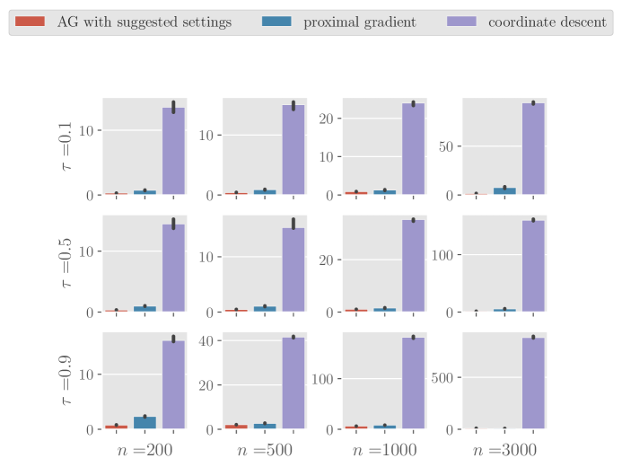
Figure 11: Median for the computing time (in seconds) required for $\left\|\bm{\beta}^{\left(k+1\right)}-\bm{\beta}^{\left(k\right)}\right\|_{\infty}$ to fall below $10^{-4}$ on MCP-penalized linear model for AG with our proposed hyperparameter settings, proximal gradient, and coordinate descent over $100$ simulation replications, across varying covariates correlation ($\tau$) and $q/n$ values. The error bars represent the $95\%$ CIs from $1000$ bootstrap replications, $g^{*}$ represents the minimum per iterate found by the three methods considered.

Figures 10, 11 report median with the corresponding $95\%$ bootstrap CI of the computing time (in seconds) required for the infinity norm of the two consecutive iterations $\left\|\bm{\beta}^{\left(k+1\right)}-\bm{\beta}^{\left(k\right)}\right\|_{\infty}$ to fall below $10^{-4}$ for $100$ simulation replications. It can be observed that the computing time for AG with suggested settings is much shorter than the computing time for coordinate descent.

Figure 3: Solution paths obtained using the proposed AG method for MCP-penalized linear model with different values of $\gamma$ for a single simulation replicate. The behaviors of the solution path match the expected from the MCP penalized problems. The solution path behaves similarly to hard-thresholding for a small $\gamma$. As $\gamma$ increases, the solution path will behave more similarly to soft-thresholding.

To visualize the signal recovery performance using our proposed method, Figure 3 plots the solution paths for the MCP-penalized linear model with different values of $\gamma$. The grey lines in Figure 3 represent the recovered values for the noise variables. AG method performs very well when applied to signal recovery problems for nonconvex-penalized linear models. Figure 3 serves as an arbitrary instance that the recovered signals using our method exhibit the expected pattern with MCP – as $\lambda$ decreases, the degree of penalization decreases, and more false-positive signals will be selected. The stable solution path for the recovered signals suggests that the algorithm does not converge to a point far away from the “true” coefficients.

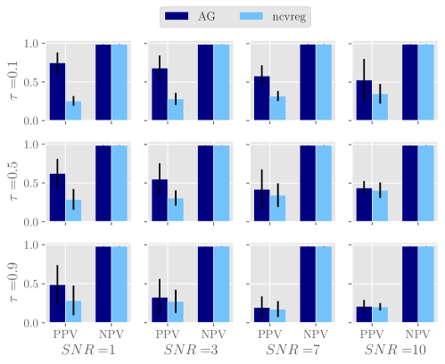
Figure 4: Sample means for Positive/Negative Predictive Values (PPV, NPV) of signal detection across different values of covariates correlation ($\tau$) and SNRs for AG with our proposed hyperparameter settings and ncvreg on SCAD-penalized linear model over $100$ simulation replications. The error bars represent the standard errors.

To further illustrate the signal recovery performance, the means and standard errors for the scaled estimation error $\frac{\left\|\bm{\beta}_{\text{true}}-\hat{\bm{\beta}}\right\|_{2}^{2}}{\left\|\bm{\beta}_{\text{true}}\right\|_{2}^{2}}$, positive/negative predictive values (PPV, NPV), and active set cardinality across $100$ replications are reported in Tables 1 and 2 in Appendix B.1. In what follows, $\mathcal{A}$ denotes the set of nonzero “true” coefficients and $\hat{\mathcal{A}}$ denotes the set of nonzero coefficients selected by the model. PPV and NPV use the following definitions:

$$\text{PPV}\coloneqq\frac{\lvert\mathcal{A}\cap\hat{\mathcal{A}}\rvert}{\lvert\hat{\mathcal{A}}\rvert},\ \text{NPV}\coloneqq\frac{\lvert\mathcal{A}^{C}\cap\hat{\mathcal{A}}^{C}\rvert}{\lvert\hat{\mathcal{A}}^{C}\rvert}.$$

Sample means and standard errors for PPV and NPV from Table 1 are further visualized in Figure 4. When applied to sparse learning problems, the signal recovery performance of our proposed method often outperforms ncvreg, the current state-of-the-art method [13], particularly in terms of the positive predictive values (PPV). This can be observed from Figure 4 and Tables 1, 2 from Appendix B.1. This observation is especially evident when the signal-to-noise ratios are low. At the same time, $\nicefrac{{\left\|\bm{\beta}_{\text{true}}-\hat{\bm{\beta}}\right\|_{2}^{2}}}{{\left\|\bm{\beta}_{\text{true}}\right\|_{2}^{2}}}$ for both methods are close. As the SNR increases, the validation set becomes more similar to the training set, causing the chosen model to have a smaller $\lambda$. The model size will therefore increase, which will decrease the value of PPV.

5.2.2 Penalized Logistic Regression

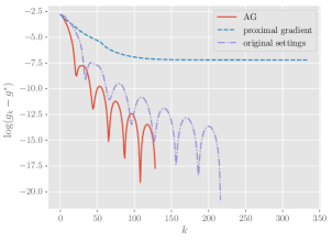
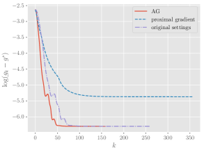
Figure 5: Convergence rate performance of first-order methods on SCAD (left) and MCP (right) penalized logistic regression for a single simulation replicate. $k$ represents the number of iterations, $g_{k}$ represents the iterative objective function value, and $g^{*}$ represent the minimum found by the three methods considered.

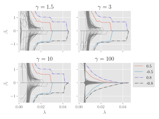
Figure 6: Solution paths obtained using the proposed AG method for MCP-penalized logistic regression with different values of $\gamma$ for a single simulation replicate. The behaviors of the solution path match the expected from the MCP penalized problems. The solution path behaves similarly to hard-thresholding for a small $\gamma$. As $\gamma$ increases, the solution path will behave more similarly to soft-thresholding.

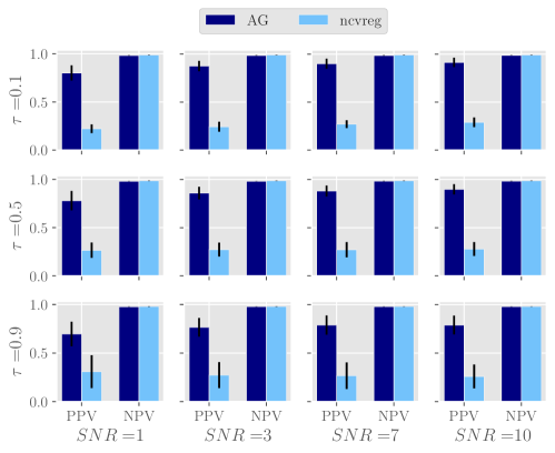
Figure 7: Sample means for Positive/Negative Predictive Values (PPV, NPV) of signal detection across different values of covariates correlation ($\tau$) and SNRs for AG with our proposed hyperparameter settings and ncvreg on SCAD-penalized logistic model over $100$ simulation replications. The error bars represent the standard error.

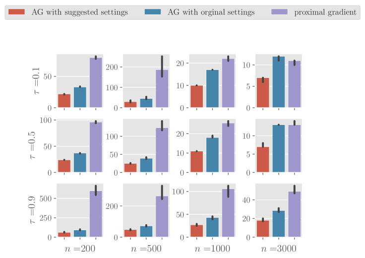
Figure 13: Median for the number of iterations required for iterative objective values to reach $g^{*}+e^{2}$ on MCP-penalized logistic regression for AG with our proposed hyperparameter settings, AG with original settings, and proximal gradient over $100$ simulation replications, across varying covariates correlation ($\tau$) and $q/n$ values. The error bars represent the $95\%$ CIs from $1000$ bootstrap replications, $g^{*}$ represents the minimum per iterate found by the three methods considered.

The simulation results reflected in Figures 5, 6, as well as Figures 12, 13 and Tables 3, 4 in Appendix B.2 suggest similar findings for penalized logistic models to our findings for penalized linear models as discussed in Section 5.2.1. We further note that when applied to penalized logistic models, the coordinate descent method often fails to converge, resulting in overall poor performance in positive predictive values as reflected in Figure 7 and Tables 3, 4 in Appendix B.2. When it does converge, the coordinate descent method does so at a very slow rate. In comparison, our proposed method has a convergence guarantee in theory and converges within a reasonable number of iterations in our simulation studies, as shown in Figures 8, 9 in Appendix B.2. In our computing time comparison, we used identical simulation setups and convergence standard for both the AG method and coordinate descent method, running both on a NVIDIA A100 GPU with CUDA compute capability of 8.0 from Compute Canada; the submitted simulation job finished well within $20$ minutes for both SCAD and MCP-penalized logistic models when using the AG method, but exceeded the 7-day computing time limit imposed on the Narval cluster when using the coordinate descent method.

6 Discussion

We considered a recently developed generalization of Nesterov’s accelerated gradient method for nonconvex optimization, and we have discussed its potential in sparse statistical learning with nonconvex penalties. An important issue concerning this algorithm is the selection of its sequences of hyperparameters. We present an explicit solution to this problem by minimizing the algorithm’s complexity upper bound, hence accelerating convergence of the algorithm. Our simulation studies indicate that among first-order methods, the AG method using our proposed hyperparameter settings achieves a convergence rate considerably faster than other first-order methods such as the AG method using the original proposed hyperparameter settings or proximal gradient. Our simulations also show that signal recovery using our proposed method generally outperforms ncvreg, the current state-of-the-art method. This performance gain is much more pronounced for penalized linear models when the signal-to-noise ratios are low. For penalized logistic regression, the performance gain observed is consistent across various covariates correlation and signal-to-noise ratio settings. Compared to coordinate-wise minimization methods, our proposed method is less challenged by low signal-to-noise ratios and is feasible to implement in parallel. Given today’s computing facilities, parallel computing is particularly meaningful for large datasets [31]. We also show this gain in parallel computing performance by comparing computing time on a GPU. Furthermore, our proposed method has weaker convergence conditions and can be applied to a class of problems that do not have an explicit solution to the coordinate-wise objective function. For example, linear mixed models for grouped or longitudinal data involve the inverse of a large covariance matrix. Decomposition of this covariance matrix is necessary to apply the coordinate descent method. However, such decomposition can be computationally costly and numerically unstable [32]. On the other hand, matrix decomposition is not needed for first-order methods, as numerically stable yet computationally efficient approaches such as conjugate gradient can be adapted when applying our proposed method. The proposed nonconvex AG method can be applied to a wide range of statistical learning problems, opening various future research opportunities in statistical machine learning and statistical genetics.

7 Disclaimer

All codes to reproduce the simulation results of this paper and outputs from Calcul Quebec/Compute Canada can be found on the following GitHub repository:

https://github.com/Kaiyangshi-Ito/nonconvexAG

Appendix A Proofs

We first establish the following Lemma needed for the proof of Theorem 1.

A.1 Proof of Theorem 1

The following lemma is needed in the proof of Theorem 1.

Lemma 1.

Assume that $\forall k=1,2,\dots,N$, the convergence conditions (8) and (9) hold, then we have the following recursive relation:

$$\alpha_{k+1}\leq\frac{1}{1+\frac{\delta_{k}/\delta_{k+1}}{\alpha_{k}}}.$$ (19)

Proof.

The convergence conditions (8) and (9) gives that $\forall k=1,2,\dots,N-1$,

$$\alpha_{k+1}\delta_{k+1}\leq\omega_{k+1}\Leftrightarrow\alpha_{k+1}\leq\frac{\omega_{k+1}}{\delta_{k+1}},\text{ and}$$

$$\frac{\alpha_{k}}{\delta_{k}\Gamma_{k}}\geq\frac{\alpha_{k+1}}{\delta_{k+1}\Gamma_{k+1}}\Leftrightarrow\frac{\alpha_{k}}{\delta_{k}}\geq\frac{\alpha_{k+1}}{\delta_{k+1}\left(1-\alpha_{k+1}\right)}\Leftrightarrow\alpha_{k+1}\leq\frac{\alpha_{k}\delta_{k+1}}{\alpha_{k}\delta_{k+1}+\delta_{k}}.$$

Following above two inequalities, we have that

$$\alpha_{k+1}\leq\min\left\{\frac{\omega_{k+1}}{\delta_{k+1}},\frac{\alpha_{k}\delta_{k+1}}{\alpha_{k}\delta_{k+1}+\delta_{k}}\right\}.$$ (20)

We observe that in (20), $\frac{\omega_{k+1}}{\delta_{k+1}}$ is monotonically decreasing with respect to $\delta_{k+1}$ on $\mathbb{R}_{+}$; while $\frac{\alpha_{k}\delta_{k+1}}{\alpha_{k}\delta_{k+1}+\delta_{k}}$ is monotonically increasing with respect to $\delta_{k+1}$ on $\mathbb{R}_{+}$. This suggests:

$$\arg\max_{\delta_{k+1}>0}\left(\min\left\{\frac{\omega_{k+1}}{\delta_{k+1}},\frac{\alpha_{k}\delta_{k+1}}{\alpha_{k}\delta_{k+1}+\delta_{k}}\right\}\right)=\left\{\frac{\omega_{k+1}+\sqrt{\omega_{k+1}^{2}+\frac{4\omega_{k+1}\delta_{k}}{\alpha_{k}}}}{2}\right\}.$$ (21)

That is, the inequality constraints conditions (8) and (9) for convergence are merely a lower bound on the vanishing rate of $\left\{\alpha_{k}\right\}$. Therefore it follows from (8) and the (necessary) optimality condition for (21) that

$$\alpha_{k+1}\leq\frac{2\omega_{k+1}}{\omega_{k+1}+\sqrt{\omega_{k+1}^{2}+\frac{4\omega_{k+1}\delta_{k}}{\alpha_{k}}}}\leq\frac{2}{1+\sqrt{1+\frac{4\delta_{k}}{\alpha_{k}\omega_{k+1}}}}=\frac{2}{1+\sqrt{1+\frac{4\delta_{k}/\delta_{k+1}}{\alpha_{k}\alpha_{k+1}}}}.$$ (22)

By simplifying (19), we have:

$$\alpha_{k+1}\leq\frac{1}{1+\frac{\delta_{k}/\delta_{k+1}}{\alpha_{k}}}.$$

∎

We now proceed with the proof of Theorem 1.

Proof.

The complexity upper bound (10) under the given conditions can be simplified as:

$$\left[\sum_{k=1}^{N}\Gamma_{k}^{-1}\omega_{k}\left(1-L_{\Psi}\omega_{k}\right)\right]^{-1}\left[\frac{\left\|x_{0}-x^{*}\right\|^{2}}{\delta_{1}}+\frac{2L_{f}}{\Gamma_{N}}\left(\left\|x^{*}\right\|^{2}+M^{2}\right)\right]$$

$$= \left[\sum_{k=1}^{N}\Gamma_{k}^{-1}\omega_{k}\left(1-L_{\Psi}\omega_{k}\right)\right]^{-1}\cdot\frac{\left\|x_{0}-x^{*}\right\|^{2}}{\delta_{1}}$$

$$= \frac{1}{\omega\left(1-L_{\Psi}\omega\right)}\left(\sum_{k=1}^{N}\Gamma_{k}^{-1}\right)^{-1}\cdot\frac{\left\|x_{0}-x^{*}\right\|^{2}}{\omega}$$

$$= \left(\sum_{k=1}^{N}\Gamma_{k}^{-1}\right)^{-1}\cdot\frac{\left\|x_{0}-x^{*}\right\|^{2}}{\omega^{2}\left(1-L_{\Psi}\omega\right)}.$$ (23)

Observe that $\left(\sum_{k=1}^{N}\Gamma_{k}^{-1}\right)^{-1}$ is monotonically decreasing with respect to $\alpha_{k}$ for all $k=1,2,\dots,N$. This property implies that (23) is minimized when $\alpha_{k}$ attains its greatest value for $k=1,2,\dots,N$.

Condition $\delta_{1}=\omega_{k}=\omega$ gives that

$$\omega_{1}=\delta_{1}=\alpha_{1}\delta_{1}.$$

Since the upper bound for $\alpha_{k+1}$ presented in (19) is monotonically increasing with respect to $\alpha_{k}$, it then follows inductively from the (necessary) optimality condition of (20) that

$$\alpha_{k+1}\leq\frac{1}{1+\frac{\delta_{k}/\delta_{k+1}}{\alpha_{k}}}=\frac{1}{1+\frac{\alpha_{k+1}}{\alpha_{k}^{2}}},$$

which simplifies to

$$\alpha_{k+1}\leq\frac{2}{1+\sqrt{1+\frac{4}{\alpha_{k}^{2}}}}.$$

While $\omega^{2}\left(1-L_{\Psi}\omega\right)$ should be maximized to minimize the value of (23), which implies the minimizer for $\omega$ is

$$\bar{\omega}=\frac{2}{3L_{\Psi}}.$$

And $\bar{\lambda}_{k+1}=\frac{\bar{\omega}}{\bar{\alpha}_{k+1}}$ follows directly form the necessary optimality condition for (20). It is trivial to check that $\left(\left\{\bar{\alpha}_{k}\right\},\left\{\bar{\delta}_{k}\right\},\bar{\omega}\right)$ is feasible under given constraints (8) and (9). ∎

A.2 Proof of Theorem 2

Proof.

Consider arbitrary $k=2,\dots,N$, then $\alpha_{k}\in\left(0,1\right)$ by definition. In the convergence conditions (8) and (9), this gives us that

$$\frac{\alpha_{k+1}}{\alpha_{k}}\leq\frac{2}{\alpha_{k}+\sqrt{\alpha_{k}^{2}+4}}\in\left(\frac{\sqrt{5}-1}{2},1\right).$$

Thus, $\left\{\alpha_{k}\right\}$ is a bounded monotonically decreasing sequence, and $\alpha_{2}\leq\frac{2}{1+\sqrt{1+\frac{4}{1^{2}}}}=\frac{\sqrt{5}-1}{2}$ further implies that $\forall k\geq 2,\ \alpha_{k}\in(0,\frac{\sqrt{5}-1}{2}]$.

For all $k\geq 2$, $\alpha_{k}\in\left(0,1\right)$ implies that $1-\alpha_{k}\in\left(0,1\right)$. Therefore, $\Gamma_{k}^{-1}=\frac{1}{\left(1-\alpha_{2}\right)\left(1-\alpha_{3}\right)\cdots\left(1-\alpha_{k}\right)}$ is monotonically increasing with respect to $k$. Thus, $\sum_{k=1}^{N}\Gamma_{k}^{-1}=O\left(N\right)$, which implies that $\left(\sum_{k=1}^{N}\Gamma_{k}^{-1}\right)^{-1}\cdot C_{1}=O\left(1/N\right)$.

Observe that

$$0<\left(\Gamma_{N}\sum_{k=1}^{N}\frac{1}{\Gamma_{k}}\right)^{-1}=\frac{1}{N\cdot\Gamma_{N}}\cdot\frac{N}{\sum_{k=1}^{N}\frac{1}{\Gamma_{k}}}$$

$$\leq\frac{1}{N\cdot\Gamma_{N}}\cdot\left(\prod_{k=1}^{N}\Gamma_{k}\right)^{\frac{1}{N}}=\frac{1}{N}\cdot\left(\prod_{k=1}^{N}\frac{\Gamma_{k}}{\Gamma_{N}}\right)^{\frac{1}{N}}$$ (24)

$$=\frac{1}{N}\cdot\left(\prod_{k=1}^{N}\frac{\Gamma_{N}}{\Gamma_{k}}\right)^{-\frac{1}{N}}=\frac{1}{N}\cdot\left(\prod_{k=2}^{N}\left(1-\alpha_{k}\right)^{k}\right)^{-\frac{1}{N}}$$

$$=\frac{1}{N}\cdot\prod_{k=2}^{N}\left(1-\alpha_{k}\right)^{-\frac{k}{N}},$$

where the inequality in (24) follows from the harmonic mean-geometric mean inequality.

Consider arbitrary $N\in\mathbb{N}$, now we are to prove that $\forall k=1,2,\dots,N,\ \alpha_{k}\leq\frac{2}{k+1}$. By definition, $\alpha_{1}=1\leq 1$. Assume that $\alpha_{k}\leq\frac{2}{k+1}$, then by the convergence conditions,

$$\alpha_{k+1}\leq \frac{2}{1+\sqrt{1+\frac{4}{\alpha_{k}^{2}}}}$$

$$\leq \frac{2}{1+\sqrt{1+4/\left(\frac{2}{k+1}\right)^{2}}}$$

$$= \frac{2}{1+\sqrt{2+2k+k^{2}}}$$

$$< \frac{2}{k+2}.$$

Thus, by mathematical induction, $\forall k=1,2,\dots,N,\ \alpha_{k}\leq\frac{2}{k+1}$. Hence, $\sum_{k=1}^{N}\frac{k}{N}\alpha_{k}<\sum_{k=1}^{N}\frac{k}{N}\cdot\frac{2}{k}=\sum_{k=1}^{N}\frac{2}{N}=2<\infty$ as $N\rightarrow\infty$.

Furthermore, we have that $\forall x\in(0,\frac{\sqrt{5}-1}{2}],\ -\log\left(1-x\right)<x$. Combined with the fact that $\forall k\geq 2,\ \alpha_{k}\in(0,\frac{\sqrt{5}-1}{2}]$, we have that $\forall k\geq 2,\ -\log\left(1-\alpha_{k}\right)<\alpha_{k}$. Thus,

$$\log\left(\prod_{k=2}^{N}\left(1-\alpha_{k}\right)^{-\frac{k}{N}}\right)=-\sum_{k=2}^{N}\frac{k}{N}\log\left(1-\alpha_{k}\right)<\sum_{k=2}^{N}\frac{k}{N}\alpha_{k}\leq 2<\infty.$$

Therefore, $\prod_{k=2}^{N}\left(1-\alpha_{k}\right)^{-\frac{k}{N}}$ is also upper bounded as $N\rightarrow\infty$, which implies that

$$\left(\sum_{k=1}^{N}\frac{\Gamma_{N}}{\Gamma_{k}}\right)^{-1}\leq\frac{1}{N}\cdot\prod_{k=2}^{N}\left(1-\alpha_{k}\right)^{-\frac{k}{N}}=O\left(1/N\right).$$

Hence, $\left(\sum_{k=1}^{N}\frac{\Gamma_{N}}{\Gamma_{k}}\right)^{-1}\cdot C_{2}=O\left(1/N\right)$. Therefore, $\left(\sum_{k=1}^{N}\Gamma_{k}^{-1}\right)^{-1}\cdot C_{1}+\left(\sum_{k=1}^{N}\frac{\Gamma_{N}}{\Gamma_{k}}\right)^{-1}\cdot C_{2}=O\left(1/N\right)$. ∎

A.3 Proof of Theorem 3

Proof.

$\bar{\alpha}_{k}\leq\frac{2}{k+1}$ for $k=1,2,\dots,N$ has already been proved in the proof of Theorem 2. For the left inequality, note that $\bar{\alpha}_{1}=1\geq\frac{2}{2+a}$ for $a>0$; for $k\geq 2$, we are to prove a stronger inequality:

$$\bar{\alpha}_{k}\geq\frac{2}{\sqrt{\left(1+a\cdot k^{-b}\right)k\left[\left(1+a\cdot k^{-b}\right)k+2\right]}}.$$ (25)

For $k=2$, condition (17) implies that

$$a\cdot 2^{-b}\geq\frac{1}{\left(1-b\right)\left(4-b\right)}>\frac{1}{4}>\sqrt{5}-2\text{ for }0<b<1,$$ (26)

which suggests $\bar{\alpha}_{2}=\frac{2}{1+\sqrt{5}}\geq\frac{2}{\sqrt{\left(1+a\cdot 2^{-b}\right)\cdot 2\left[\left(1+a\cdot 2^{-b}\right)\cdot 2+2\right]}}$ by simple algebra. Assume (25) holds for $k=t$, then

$$\bar{\alpha}_{t+1}= \frac{2}{1+\sqrt{1+\frac{4}{\bar{\alpha}_{t}^{2}}}}$$

$$\geq \frac{2}{1+\sqrt{1+4/\left(2/\sqrt{\left(1+a\cdot t^{-b}\right)t\left[\left(1+a\cdot t^{-b}\right)t+2\right]}\right)^{2}}}$$

$$= \frac{2}{1+\sqrt{1+\left(1+a\cdot t^{-b}\right)t\left[\left(1+a\cdot t^{-b}\right)t+2\right]}}$$

$$= \frac{2}{\left(1+a\cdot t^{-b}\right)t+2}$$

$$\geq \frac{2}{\sqrt{\left(1+a\cdot\left(t+1\right)^{-b}\right)\left(t+1\right)\left[\left(1+a\cdot\left(t+1\right)^{-b}\right)\left(t+1\right)+2\right]}};$$ (27)

and (27) follows from

$$\left(1+a\cdot\left(t+1\right)^{-b}\right)\left(t+1\right)\left[\left(1+a\cdot\left(t+1\right)^{-b}\right)\left(t+1\right)+2\right]-\left[\left(1+a\cdot t^{-b}\right)t+2\right]^{2}$$

$$= a^{2}\left[\left(t+1\right)^{2-2b}-t^{2-2b}\right]+2at\left[\left(t+1\right)^{1-b}-t^{1-b}\right]+4a\left[\left(t+1\right)^{1-b}-t^{1-b}\right]-1$$

$$\geq 2at\left[\left(t+1\right)^{1-b}-t^{1-b}\right]-1$$

$$= 2at^{2-b}\left[\left(1+\frac{1}{t}\right)^{1-b}-1\right]-1$$

$$\geq 2at^{2-b}\left[1+\left(1+b\right)t^{-1}-\frac{1}{2}b\left(1-b\right)t^{-2}-1\right]-1$$ (28)

$$= 2a\left(1-b\right)t^{1-b}-ab\left(1-b\right)t^{-b}-1\geq 0.$$ (29)

(28) follows from binomial approximation inequality; $a>0$ and $0<b<1$ suggest that $2a\left(1-b\right)k^{1-b}-ab\left(1-b\right)k^{-b}-1$ is monotonically increasing with respect to $k$ for $k>0$, condition (17) therefore implies that $2a\left(1-b\right)k^{1-b}-ab\left(1-b\right)k^{-b}-1\geq 0$ for all $k\geq 2$, which is (29).

And proof of the left inequality for $k\geq 2$ proceeds as the following:

$$\bar{\alpha}_{k}\geq \frac{2}{\sqrt{\left(1+a\cdot k^{-b}\right)k\left[\left(1+a\cdot k^{-b}\right)k+2\right]}}$$

$$> \frac{2}{\sqrt{\left(1+a\cdot k^{-b}\right)k\left[\left(1+a\cdot k^{-b}\right)k+2\right]+1}}$$

$$= \frac{2}{\left(1+a\cdot k^{-b}\right)k+1}.$$

∎

A.4 Proof of Corollary 1

Proof.

Observe that the lower bound of (16) is monotonically decreasing with respect to $a$ under given conditions. Constraint (17) implies (26), which further suggests that

$$a\geq\frac{2^{b}}{\left(1-b\right)\left(4-b\right)}>0\text{ for }0<b<1;$$

i.e., $\bar{a}_{k}=\frac{\left(2/k\right)^{\bar{b}_{k}}}{\left(1-\bar{b}_{k}\right)\left(4-\bar{b}_{k}\right)}$. Thus, maximizing the lower bound of (16) is equivalent to minimize the convex function $\log\frac{\left(2/k\right)^{b}}{\left(1-b\right)\left(4-b\right)}$ with respect to $b$ over a open set $\left(0,1\right)$. First-order sufficient optimality condition gives the unique optimizer

$$\bar{b}_{k}=\frac{2+5\left(\log\frac{2}{k}\right)+\sqrt{9\left(\log\frac{2}{k}\right)^{2}+4}}{2\left(\log\frac{2}{k}\right)}\in\left(0,1\right)$$

for $k\geq 8$. Simple algebra shows that $\lim_{k\rightarrow\infty}\frac{\bar{a}_{k}k^{1-\bar{b}_{k}}}{\log k}=\frac{2}{3}e$. Thus, the lower bound in Theorem 3 becomes $\frac{k+1}{2}-\bar{\alpha}_{k}^{-1}=O\left(\log k\right)$. ∎

Appendix B Further Simulations

B.1 Penalized Linear Model

In Figure 8 and 9, the red bar represents AG using our proposed hyperparameter settings, blue bar represents proximal gradient, and the purple bar represents AG using the original hyperparameter settings [25]. It is evident that for penalized linear models, AG using our hyperparameter settings outperforms proximal gradient or AG using the original proposed hyperparameter settings considerably.

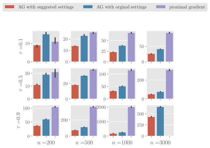
Figure 8: Median for the number of iterations required for the iterative objective value to reach $g^{*}+e^{3}$ on SCAD-penalized linear model for AG with our proposed hyperparameter settings, AG with original settings, and proximal gradient over $100$ simulation replications, across varying covariates correlation ($\tau$) and $q/n$ values. The error bars represent the $95\%$ CIs from $1000$ bootstrap replications, $g^{*}$ represents the minimum per iterate found by the three methods considered.

In Figure 10 and 11, the red bar represents AG using our proposed hyperparameter settings, blue bar represents proximal gradient, and the purple bar represents coordinate descent. It is evident that for penalized linear models, AG using our hyperparameter settings outperforms coordinate descent significantly in terms of computing time.

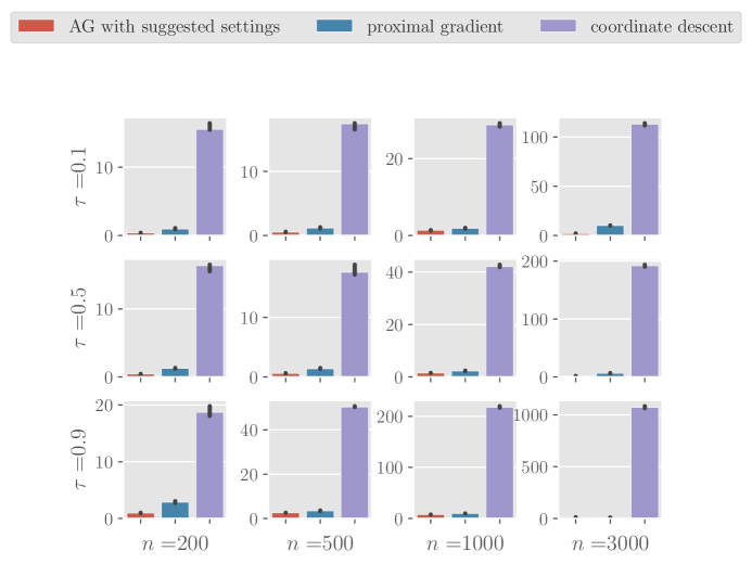
Figure 10: Median for the computing time (in seconds) required for $\left\|\bm{\beta}^{\left(k+1\right)}-\bm{\beta}^{\left(k\right)}\right\|_{\infty}$ to fall below $10^{-4}$ on SCAD-penalized linear model for AG with our proposed hyperparameter settings, proximal gradient, and coordinate descent over $100$ simulation replications, across varying covariates correlation ($\tau$) and $q/n$ values. The error bars represent the $95\%$ CIs from $1000$ bootstrap replications, $g^{*}$ represents the minimum per iterate found by the three methods considered.

Table 1: Signal recovery performance (sample mean and standard error of $\nicefrac{{\left\|\bm{\beta}_{\text{true}}-\hat{\bm{\beta}}\right\|_{2}^{2}}}{{\left\|\bm{\beta}_{\text{true}}\right\|_{2}^{2}}}$, Positive/Negative Predictive Values (PPV, NPV) for signal detection, and active set cardinality $\lvert\hat{\mathcal{A}}\rvert$) for ncvreg and AG with our proposed hyperparameter settings on SCAD-penalized linear model over $100$ simulation replications, across varying values of SNRs and covariates correlations ($\tau$).

$\nicefrac{{\left\|\bm{\beta}_{\text{true}}-\hat{\bm{\beta}}\right\|_{2}^{2}}}{{\left\|\bm{\beta}_{\text{true}}\right\|_{2}^{2}}}$	$\tau=0.1$	$0.5$	$0.9$
$\text{SNR}=1$, AG	$0.128(0.021)$	$0.521(0.114)$	$2.839(0.497)$
$\text{SNR}=1$, ncvreg	$0.131(0.02)$	$0.485(0.102)$	$2.929(0.525)$
$\text{SNR}=3$, AG	$0.05(0.009)$	$0.156(0.035)$	$2.075(0.339)$
$\text{SNR}=3$, ncvreg	$0.052(0.009)$	$0.156(0.028)$	$2.087(0.357)$
$\text{SNR}=7$, AG	$0.022(0.004)$	$0.085(0.014)$	$1.278(0.262)$
$\text{SNR}=7$, ncvreg	$0.021(0.004)$	$0.083(0.015)$	$1.3(0.262)$
$\text{SNR}=10$, AG	$0.016(0.003)$	$0.065(0.011)$	$1.163(0.207)$
$\text{SNR}=10$, ncvreg	$0.015(0.003)$	$0.063(0.013)$	$1.167(0.22)$
PPV	$\tau=0.1$	$0.5$	$0.9$
$\text{SNR}=1$, AG	$0.747(0.134)$	$0.622(0.188)$	$0.488(0.25)$
$\text{SNR}=1$, ncvreg	$0.255(0.061)$	$0.287(0.132)$	$0.286(0.19)$
$\text{SNR}=3$, AG	$0.681(0.162)$	$0.551(0.206)$	$0.327(0.234)$
$\text{SNR}=3$, ncvreg	$0.282(0.079)$	$0.307(0.098)$	$0.275(0.148)$
$\text{SNR}=7$, AG	$0.58(0.138)$	$0.42(0.257)$	$0.197(0.141)$
$\text{SNR}=7$, ncvreg	$0.32(0.065)$	$0.344(0.152)$	$0.175(0.101)$
$\text{SNR}=10$, AG	$0.528(0.272)$	$0.437(0.09)$	$0.211(0.081)$
$\text{SNR}=10$, ncvreg	$0.349(0.127)$	$0.409(0.1)$	$0.206(0.047)$
NPV	$\tau=0.1$	$0.5$	$0.9$
$\text{SNR}=1$, AG	$0.984(0.001)$	$0.984(0.001)$	$0.979(0.001)$
$\text{SNR}=1$, ncvreg	$0.987(0.001)$	$0.986(0.001)$	$0.98(0.001)$
$\text{SNR}=3$, AG	$0.989(0.001)$	$0.988(0.002)$	$0.98(0.001)$
$\text{SNR}=3$, ncvreg	$0.99(0.001)$	$0.989(0.001)$	$0.98(0.001)$
$\text{SNR}=7$, AG	$0.992(0.001)$	$0.991(0.001)$	$0.981(0.001)$
$\text{SNR}=7$, ncvreg	$0.993(0.001)$	$0.991(0.001)$	$0.981(0.001)$
$\text{SNR}=10$, AG	$0.993(0.001)$	$0.992(0.001)$	$0.982(0.001)$
$\text{SNR}=10$, ncvreg	$0.993(0.001)$	$0.992(0.001)$	$0.982(0.001)$
$\lvert\hat{\mathcal{A}}\rvert$	$\tau=0.1$	$0.5$	$0.9$
$\text{SNR}=1$, AG	$25.82(8.08)$	$31.58(17.056)$	$23.11(15.166)$
$\text{SNR}=1$, ncvreg	$100.88(25.582)$	$94.32(41.572)$	$42.01(20.592)$
$\text{SNR}=3$, AG	$42.78(14.003)$	$55.48(20.653)$	$42.83(16.308)$
$\text{SNR}=3$, ncvreg	$120.17(33.554)$	$101.75(29.498)$	$46.72(16.252)$
$\text{SNR}=7$, AG	$61.89(21.881)$	$97.88(36.736)$	$86.71(26.567)$
$\text{SNR}=7$, ncvreg	$115.4(23.845)$	$107.19(31.445)$	$89.74(23.1)$
$\text{SNR}=10$, AG	$101.21(66.968)$	$81.17(25.325)$	$70.8(11.642)$
$\text{SNR}=10$, ncvreg	$123.5(52.077)$	$90.58(40.419)$	$71.47(10.954)$

Table 2: Signal recovery performance (sample mean and standard error of $\nicefrac{{\left\|\bm{\beta}_{\text{true}}-\hat{\bm{\beta}}\right\|_{2}^{2}}}{{\left\|\bm{\beta}_{\text{true}}\right\|_{2}^{2}}}$, Positive/Negative Predictive Values (PPV, NPV), and active set cardinality $\lvert\hat{\mathcal{A}}\rvert$ for signal detection) for ncvreg and AG with our proposed hyperparameter settings on MCP-penalized linear model over $100$ simulation replications, across varying values of SNRs and covariates correlations ($\tau$).

$\nicefrac{{\left\|\bm{\beta}_{\text{true}}-\hat{\bm{\beta}}\right\|_{2}^{2}}}{{\left\|\bm{\beta}_{\text{true}}\right\|_{2}^{2}}}$	$\tau=0.1$	$0.5$	$0.9$
$\text{SNR}=1$, AG	$0.133(0.022)$	$0.563(0.124)$	$2.839(0.39)$
$\text{SNR}=1$, ncvreg	$0.126(0.019)$	$0.494(0.112)$	$2.86(0.427)$
$\text{SNR}=3$, AG	$0.049(0.01)$	$0.169(0.034)$	$1.997(0.329)$
$\text{SNR}=3$, ncvreg	$0.048(0.009)$	$0.161(0.032)$	$1.92(0.34)$
$\text{SNR}=7$, AG	$0.021(0.004)$	$0.088(0.016)$	$1.503(0.329)$
$\text{SNR}=7$, ncvreg	$0.02(0.004)$	$0.086(0.017)$	$1.416(0.302)$
$\text{SNR}=10$, AG	$0.014(0.003)$	$0.059(0.011)$	$1.084(0.272)$
$\text{SNR}=10$, ncvreg	$0.014(0.003)$	$0.059(0.013)$	$1.134(0.248)$
PPV	$\tau=0.1$	$0.5$	$0.9$
$\text{SNR}=1$, AG	$0.85(0.081)$	$0.744(0.161)$	$0.616(0.208)$
$\text{SNR}=1$, ncvreg	$0.435(0.085)$	$0.407(0.135)$	$0.387(0.154)$
$\text{SNR}=3$, AG	$0.842(0.119)$	$0.732(0.21)$	$0.506(0.286)$
$\text{SNR}=3$, ncvreg	$0.505(0.112)$	$0.514(0.121)$	$0.366(0.18)$
$\text{SNR}=7$, AG	$0.761(0.175)$	$0.646(0.293)$	$0.505(0.218)$
$\text{SNR}=7$, ncvreg	$0.541(0.128)$	$0.547(0.173)$	$0.483(0.201)$
$\text{SNR}=10$, AG	$0.801(0.099)$	$0.489(0.134)$	$0.375(0.225)$
$\text{SNR}=10$, ncvreg	$0.559(0.107)$	$0.476(0.135)$	$0.377(0.225)$
NPV	$\tau=0.1$	$0.5$	$0.9$
$\text{SNR}=1$, AG	$0.983(0.001)$	$0.982(0.001)$	$0.979(0.001)$
$\text{SNR}=1$, ncvreg	$0.986(0.001)$	$0.984(0.001)$	$0.979(0.0)$
$\text{SNR}=3$, AG	$0.988(0.001)$	$0.986(0.001)$	$0.98(0.001)$
$\text{SNR}=3$, ncvreg	$0.989(0.001)$	$0.987(0.001)$	$0.98(0.001)$
$\text{SNR}=7$, AG	$0.991(0.001)$	$0.989(0.001)$	$0.981(0.001)$
$\text{SNR}=7$, ncvreg	$0.992(0.001)$	$0.989(0.001)$	$0.981(0.001)$
$\text{SNR}=10$, AG	$0.992(0.001)$	$0.99(0.001)$	$0.982(0.001)$
$\text{SNR}=10$, ncvreg	$0.993(0.001)$	$0.99(0.001)$	$0.982(0.001)$
$\lvert\hat{\mathcal{A}}\rvert$	$\tau=0.1$	$0.5$	$0.9$
$\text{SNR}=1$, AG	$19.7(4.584)$	$20.6(9.45)$	$12.5(8.163)$
$\text{SNR}=1$, ncvreg	$51.61(13.612)$	$47.32(16.093)$	$20.25(11.411)$
$\text{SNR}=3$, AG	$30.55(8.437)$	$34.52(16.44)$	$25.37(14.373)$
$\text{SNR}=3$, ncvreg	$60.14(15.873)$	$48.08(13.783)$	$31.0(13.981)$
$\text{SNR}=7$, AG	$44.45(14.273)$	$56.95(32.804)$	$31.96(25.048)$
$\text{SNR}=7$, ncvreg	$66.7(20.364)$	$58.36(24.633)$	$33.38(25.617)$
$\text{SNR}=10$, AG	$43.23(11.26)$	$64.65(12.923)$	$46.58(18.186)$
$\text{SNR}=10$, ncvreg	$65.36(13.06)$	$67.16(15.483)$	$46.07(19.223)$

B.2 Penalized Logistic Regression

Figure (12) and (13) suggest that much less iterations are needed for our method to achieve the same amount of descent in comparison of AG with original proposed settings for penalized logistic models.

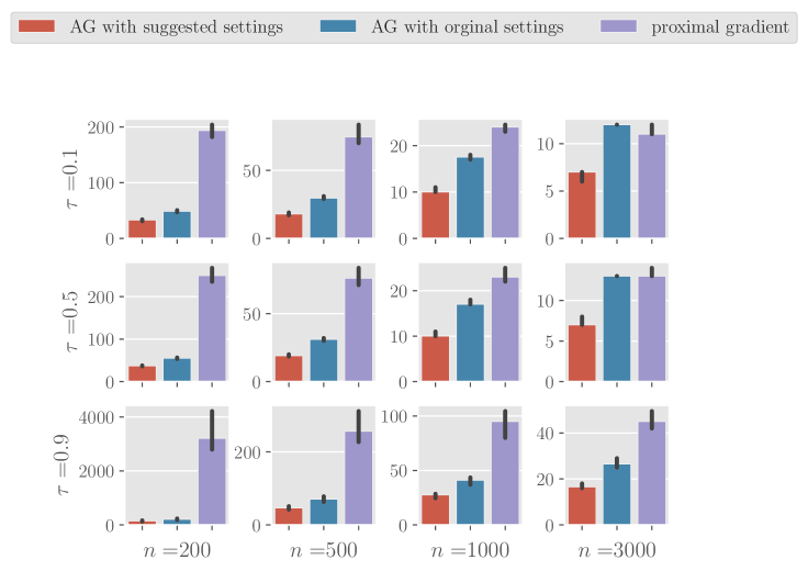
Figure 12: Median for the number of iterations required for the iterative objective values to reach $g^{*}+e^{2}$ on SCAD-penalized logistic regression for AG with our proposed hyperparameter settings, AG with original settings, and proximal gradient over $100$ simulation replications, across varying covariates correlation ($\tau$) and $q/n$ values. The error bars represent the $95\%$ CIs from $1000$ bootstrap replications, $g^{*}$ represents the minimum per iterate found by the three methods considered.

Table 3: Signal recovery performance (sample mean and standard error of $\nicefrac{{\left\|\bm{\beta}_{\text{true}}-\hat{\bm{\beta}}\right\|_{2}^{2}}}{{\left\|\bm{\beta}_{\text{true}}\right\|_{2}^{2}}}$, Positive/Negative Predictive Values (PPV, NPV), and active set cardinality $\lvert\hat{\mathcal{A}}\rvert$ for signal detection) for ncvreg and AG with our proposed hyperparameter settings on SCAD-penalized logistic model over $100$ simulation replications, across varying values of SNRs and covariates correlations ($\tau$).

$\nicefrac{{\left\|\bm{\beta}_{\text{true}}-\hat{\bm{\beta}}\right\|_{2}^{2}}}{{\left\|\bm{\beta}_{\text{true}}\right\|_{2}^{2}}}$	$\tau=0.1$	$0.5$	$0.9$
$\text{SNR}=1$, AG	$0.768(0.047)$	$0.81(0.041)$	$0.896(0.04)$
$\text{SNR}=1$, ncvreg	$0.803(0.033)$	$0.84(0.033)$	$0.903(0.037)$
$\text{SNR}=3$, AG	$0.556(0.057)$	$0.656(0.054)$	$0.839(0.056)$
$\text{SNR}=3$, ncvreg	$0.603(0.053)$	$0.682(0.055)$	$0.813(0.053)$
$\text{SNR}=7$, AG	$0.377(0.076)$	$0.521(0.073)$	$0.779(0.072)$
$\text{SNR}=7$, ncvreg	$0.438(0.054)$	$0.537(0.074)$	$0.735(0.074)$
$\text{SNR}=10$, AG	$0.311(0.077)$	$0.474(0.073)$	$0.757(0.079)$
$\text{SNR}=10$, ncvreg	$0.377(0.064)$	$0.481(0.079)$	$0.712(0.078)$
PPV	$\tau=0.1$	$0.5$	$0.9$
$\text{SNR}=1$, AG	$0.8(0.079)$	$0.779(0.1)$	$0.697(0.126)$
$\text{SNR}=1$, ncvreg	$0.221(0.045)$	$0.265(0.079)$	$0.309(0.169)$
$\text{SNR}=3$, AG	$0.875(0.054)$	$0.859(0.065)$	$0.765(0.096)$
$\text{SNR}=3$, ncvreg	$0.244(0.052)$	$0.273(0.072)$	$0.273(0.133)$
$\text{SNR}=7$, AG	$0.901(0.052)$	$0.881(0.057)$	$0.788(0.098)$
$\text{SNR}=7$, ncvreg	$0.27(0.04)$	$0.271(0.079)$	$0.267(0.136)$
$\text{SNR}=10$, AG	$0.915(0.048)$	$0.899(0.054)$	$0.789(0.097)$
$\text{SNR}=10$, ncvreg	$0.29(0.05)$	$0.279(0.072)$	$0.26(0.123)$
NPV	$\tau=0.1$	$0.5$	$0.9$
$\text{SNR}=1$, AG	$0.982(0.001)$	$0.98(0.001)$	$0.978(0.001)$
$\text{SNR}=1$, ncvreg	$0.987(0.002)$	$0.985(0.002)$	$0.98(0.001)$
$\text{SNR}=3$, AG	$0.985(0.002)$	$0.982(0.001)$	$0.979(0.001)$
$\text{SNR}=3$, ncvreg	$0.99(0.002)$	$0.987(0.002)$	$0.98(0.001)$
$\text{SNR}=7$, AG	$0.987(0.002)$	$0.984(0.001)$	$0.979(0.001)$
$\text{SNR}=7$, ncvreg	$0.992(0.001)$	$0.988(0.001)$	$0.98(0.001)$
$\text{SNR}=10$, AG	$0.988(0.002)$	$0.984(0.001)$	$0.979(0.001)$
$\text{SNR}=10$, ncvreg	$0.992(0.001)$	$0.988(0.001)$	$0.98(0.001)$
$\lvert\hat{\mathcal{A}}\rvert$	$\tau=0.1$	$0.5$	$0.9$
$\text{SNR}=1$, AG	$17.07(3.91)$	$13.4(3.365)$	$7.62(2.134)$
$\text{SNR}=1$, ncvreg	$120.14(28.882)$	$86.49(24.421)$	$39.41(19.448)$
$\text{SNR}=3$, AG	$23.34(4.203)$	$16.59(3.459)$	$8.69(2.082)$
$\text{SNR}=3$, ncvreg	$134.85(29.96)$	$98.48(28.434)$	$42.47(15.014)$
$\text{SNR}=7$, AG	$26.98(4.58)$	$19.46(3.659)$	$9.79(2.246)$
$\text{SNR}=7$, ncvreg	$130.33(22.255)$	$105.03(28.123)$	$48.81(19.059)$
$\text{SNR}=10$, AG	$27.95(4.462)$	$19.57(3.141)$	$10.24(2.346)$
$\text{SNR}=10$, ncvreg	$124.58(23.016)$	$103.49(27.66)$	$50.64(21.138)$

Table 4: Signal recovery performance (sample mean and standard error of $\nicefrac{{\left\|\bm{\beta}_{\text{true}}-\hat{\bm{\beta}}\right\|_{2}^{2}}}{{\left\|\bm{\beta}_{\text{true}}\right\|_{2}^{2}}}$, Positive/Negative Predictive Values (PPV, NPV), and active set cardinality $\lvert\hat{\mathcal{A}}\rvert$ for signal detection) for ncvreg and AG with our proposed hyperparameter settings on MCP-penalized logistic model over $100$ simulation replications, across varying values of SNRs and covariates correlations ($\tau$).

$\nicefrac{{\left\|\bm{\beta}_{\text{true}}-\hat{\bm{\beta}}\right\|_{2}^{2}}}{{\left\|\bm{\beta}_{\text{true}}\right\|_{2}^{2}}}$	$\tau=0.1$	$0.5$	$0.9$
$\text{SNR}=1$, AG	$0.769(0.044)$	$0.808(0.041)$	$0.897(0.043)$
$\text{SNR}=1$, ncvreg	$0.795(0.036)$	$0.829(0.032)$	$0.903(0.038)$
$\text{SNR}=3$, AG	$0.555(0.058)$	$0.654(0.053)$	$0.834(0.054)$
$\text{SNR}=3$, ncvreg	$0.605(0.049)$	$0.674(0.054)$	$0.825(0.057)$
$\text{SNR}=7$, AG	$0.383(0.08)$	$0.521(0.069)$	$0.779(0.07)$
$\text{SNR}=7$, ncvreg	$0.438(0.057)$	$0.533(0.07)$	$0.761(0.071)$
$\text{SNR}=10$, AG	$0.31(0.079)$	$0.469(0.073)$	$0.753(0.076)$
$\text{SNR}=10$, ncvreg	$0.381(0.061)$	$0.48(0.082)$	$0.737(0.077)$
PPV	$\tau=0.1$	$0.5$	$0.9$
$\text{SNR}=1$, AG	$0.879(0.06)$	$0.859(0.058)$	$0.779(0.087)$
$\text{SNR}=1$, ncvreg	$0.372(0.068)$	$0.401(0.106)$	$0.375(0.157)$
$\text{SNR}=3$, AG	$0.906(0.05)$	$0.889(0.05)$	$0.805(0.086)$
$\text{SNR}=3$, ncvreg	$0.43(0.065)$	$0.445(0.106)$	$0.395(0.126)$
$\text{SNR}=7$, AG	$0.919(0.044)$	$0.903(0.05)$	$0.809(0.102)$
$\text{SNR}=7$, ncvreg	$0.463(0.063)$	$0.45(0.104)$	$0.417(0.145)$
$\text{SNR}=10$, AG	$0.918(0.045)$	$0.911(0.038)$	$0.804(0.111)$
$\text{SNR}=10$, ncvreg	$0.502(0.069)$	$0.468(0.095)$	$0.412(0.137)$
NPV	$\tau=0.1$	$0.5$	$0.9$
$\text{SNR}=1$, AG	$0.981(0.001)$	$0.98(0.001)$	$0.978(0.001)$
$\text{SNR}=1$, ncvreg	$0.986(0.002)$	$0.983(0.001)$	$0.978(0.001)$
$\text{SNR}=3$, AG	$0.985(0.002)$	$0.982(0.001)$	$0.979(0.001)$
$\text{SNR}=3$, ncvreg	$0.989(0.002)$	$0.985(0.001)$	$0.979(0.001)$
$\text{SNR}=7$, AG	$0.987(0.002)$	$0.984(0.001)$	$0.98(0.001)$
$\text{SNR}=7$, ncvreg	$0.991(0.002)$	$0.986(0.001)$	$0.98(0.001)$
$\text{SNR}=10$, AG	$0.988(0.002)$	$0.984(0.001)$	$0.98(0.001)$
$\text{SNR}=10$, ncvreg	$0.991(0.001)$	$0.987(0.001)$	$0.98(0.001)$

$\lvert\hat{\mathcal{A}}\rvert$	$\tau=0.1$	$0.5$	$0.9$
$\text{SNR}=1$, AG	$13.86(3.082)$	$11.42(2.776)$	$6.72(1.744)$
$\text{SNR}=1$, ncvreg	$59.83(14.138)$	$42.1(12.546)$	$19.72(8.393)$
$\text{SNR}=3$, AG	$21.86(4.313)$	$15.84(3.036)$	$8.84(1.938)$
$\text{SNR}=3$, ncvreg	$66.57(13.203)$	$48.28(14.5)$	$22.81(9.784)$
$\text{SNR}=7$, AG	$25.75(4.776)$	$18.78(3.189)$	$10.33(2.565)$
$\text{SNR}=7$, ncvreg	$69.44(11.876)$	$52.54(13.638)$	$24.63(8.741)$
$\text{SNR}=10$, AG	$27.53(4.649)$	$19.55(3.093)$	$11.06(2.877)$
$\text{SNR}=10$, ncvreg	$65.38(10.776)$	$51.66(12.785)$	$25.59(9.428)$

References

- [1] Robert Tibshirani “Regression Shrinkage and Selection via the Lasso” In Journal of the Royal Statistical Society. Series B (Methodological) 58.1 [Royal Statistical Society, Wiley], 1996, pp. 267–288 URL: http://www.jstor.org/stable/2346178
- [2] Hui Zou and Trevor Hastie “Regularization and Variable Selection via the Elastic Net” In Journal of the Royal Statistical Society. Series B (Statistical Methodology) 67.2 [Royal Statistical Society, Wiley], 2005, pp. 301–320 URL: http://www.jstor.org/stable/3647580
- [3] Jianqing Fan and Runze Li “Variable Selection via Nonconcave Penalized Likelihood and Its Oracle Properties” In Journal of the American Statistical Association 96.456 [American Statistical Association, Taylor & Francis, Ltd.], 2001, pp. 1348–1360 URL: http://www.jstor.org/stable/3085904
- [4] Cun-Hui Zhang “Nearly unbiased variable selection under minimax concave penalty” In Annals of Statistics 2010, Vol. 38, No. 2, 894-942, 2010 DOI: 10.1214/09-AOS729
- [5] Hui Zou and Runze Li “One-Step Sparse Estimates in Nonconcave Penalized Likelihood Models” In The Annals of Statistics 36.4 Institute of Mathematical Statistics, 2008, pp. 1509–1533 URL: http://www.jstor.org/stable/25464679
- [6] Yongdai Kim, Hosik Choi and Hee-Seok Oh “Smoothly Clipped Absolute Deviation on High Dimensions” In Journal of the American Statistical Association 103.484 [American Statistical Association, Taylor & Francis, Ltd.], 2008, pp. 1665–1673 URL: http://www.jstor.org/stable/27640214
- [7] Lan Wang, Yongdai Kim and Runze Li “Calibrating nonconvex penalized regression in ultra-high dimension” In Annals of Statistics 2013, Vol. 41, No. 5, 2505-2536, 2013 DOI: 10.1214/13-AOS1159
- [8] Yurii Nesterov “Introductory Lectures on Convex Optimization” Springer US, 2004 DOI: 10.1007/978-1-4419-8853-9
- [9] Alan Edelman “Eigenvalues and Condition Numbers of Random Matrices” In SIAM Journal on Matrix Analysis and Applications 9.4 Society for Industrial & Applied Mathematics (SIAM), 1988, pp. 543–560 DOI: 10.1137/0609045
- [10] Sangin Lee, Sunghoon Kwon and Yongdai Kim “A Modified Local Quadratic Approximation Algorithm for Penalized Optimization Problems” In Comput. Stat. Data Anal. 94.C Amsterdam, The Netherlands, The Netherlands: Elsevier Science Publishers B. V., 2016, pp. 275–286 DOI: 10.1016/j.csda.2015.08.019
- [11] Sidi Zakari Ibrahim, Mkhadri Abdallah and Assi N’Guessan “A mixture of local and quadratic approximation variable selection algorithm in nonconcave penalized regression” In ARIMA 15, 2012, pp. 18
- [12] Abhik Ghosh and Magne Thoresen “Non-Concave Penalization in Linear Mixed-Effects Models and Regularized Selection of Fixed Effects” In AStA Advances in Statistical Analysis (2018), Volume 102, Issue 2, pp 179–210, 2016 DOI: 10.1007/s10182-017-0298-z
- [13] Patrick Breheny and Jian Huang “Coordinate descent algorithms for nonconvex penalized regression, with applications to biological feature selection” In Annals of Applied Statistics 2011, Vol. 5, No. 1, 232-253, 2011 DOI: 10.1214/10-AOAS388
- [14] Rahul Mazumder, Jerome H. Friedman and Trevor Hastie “SparseNet: Coordinate Descent With Nonconvex Penalties” In Journal of the American Statistical Association 106.495 [American Statistical Association, Taylor & Francis, Ltd.], 2011, pp. 1125–1138 URL: http://www.jstor.org/stable/23427579
- [15] Jerome Friedman, Trevor Hastie, Holger Höfling and Robert Tibshirani “Pathwise coordinate optimization” In Annals of Applied Statistics 2007, Vol. 1, No. 2, 302-332, 2007 DOI: 10.1214/07-AOAS131
- [16] James C. Spall “Cyclic Seesaw Process for Optimization and Identification” Springer ScienceBusiness Media LLC, 2012, pp. 187–208 DOI: 10.1007/s10957-012-0001-1
- [17] Amir Beck “First-order methods in optimization” Philadelphia Philadelphia: Society for IndustrialApplied Mathematics Mathematical Optimization Society, 2017
- [18] Y.. Nesterov “A method for solving the convex programming problem with convergence rate ” In Dokl. Akad. Nauk SSSR 269, 1983, pp. 543–547 URL: https://ci.nii.ac.jp/naid/10029946121/en/
- [19] Yurii Nesterov “Gradient methods for minimizing composite functions” In Mathematical Programming 140.1 Springer ScienceBusiness Media LLC, 2012, pp. 125–161 DOI: 10.1007/s10107-012-0629-5
- [20] Guanghui Lan “An optimal method for stochastic composite optimization” In Mathematical Programming 133.1-2 Springer ScienceBusiness Media LLC, 2011, pp. 365–397 DOI: 10.1007/s10107-010-0434-y
- [21] Noah Simon, Jerome Friedman, Trevor Hastie and Robert Tibshirani “A Sparse-Group Lasso” In Journal of Computational and Graphical Statistics 22.2 Informa UK Limited, 2013, pp. 231–245 DOI: 10.1080/10618600.2012.681250
- [22] Yi Yang and Hui Zou “A fast unified algorithm for solving group-lasso penalize learning problems” In Statistics and Computing 25.6 Springer ScienceBusiness Media LLC, 2014, pp. 1129–1141 DOI: 10.1007/s11222-014-9498-5
- [23] Donghyeon Yu et al. “High-Dimensional Fused Lasso Regression Using Majorization–Minimization and Parallel Processing” In Journal of Computational and Graphical Statistics 24.1 Informa UK Limited, 2015, pp. 121–153 DOI: 10.1080/10618600.2013.878662
- [24] Ömer Deniz Akyildiz and Joaquín Míguez “Convergence rates for optimised adaptive importance samplers” In Statistics and Computing 31.2 Springer ScienceBusiness Media LLC, 2021 DOI: 10.1007/s11222-020-09983-1
- [25] Saeed Ghadimi and Guanghui Lan “Accelerated gradient methods for nonconvex nonlinear and stochastic programming” In Mathematical Programming 156.1-2 Springer ScienceBusiness Media LLC, 2015, pp. 59–99 DOI: 10.1007/s10107-015-0871-8
- [26] Elizabeth Meckes “The Eigenvalues of Random Matrices” In IMAGE, the Bulletin of the International Linear Algebra Society, no. 65, pp. 9-22, 2020, 2021 arXiv:2101.02928 [math.PR]
- [27] Sangin Lee and Patrick Breheny “Strong Rules for Nonconvex Penalties and Their Implications for Efficient Algorithms in High-Dimensional Regression” In Journal of Computational and Graphical Statistics 24.4 Informa UK Limited, 2015, pp. 1074–1091 DOI: 10.1080/10618600.2014.975231
- [28] Chi Jin, Praneeth Netrapalli and Michael I. Jordan “Accelerated Gradient Descent Escapes Saddle Points Faster than Gradient Descent”, 2017 arXiv:1711.10456 [cs.LG]
- [29] Weijie Su, Stephen Boyd and Emmanuel J. Candès “A Differential Equation for Modeling Nesterov’s Accelerated Gradient Method: Theory and Insights” In Proceedings of the 27th International Conference on Neural Information Processing Systems - Volume 2, NIPS’14 Montreal, Canada: MIT Press, 2014, pp. 2510–2518
- [30] Courtney Paquette, Bart Merriënboer, Elliot Paquette and Fabian Pedregosa “Halting Time is Predictable for Large Models: A Universality Property and Average-case Analysis”, 2020 arXiv:2006.04299 [math.OC]
- [31] Thomas Parnell et al. “Tera-scale coordinate descent on GPUs” In Future Generation Computer Systems 108 Elsevier BV, 2020, pp. 1173–1191 DOI: 10.1016/j.future.2018.04.072
- [32] Alfio Quarteroni “Numerical mathematics” New York: Springer, 2000