Automating Outlier Detection via Meta-Learning

Abstract

Given an unsupervised outlier detection (OD) task on a new dataset, how can we automatically select a good outlier detection method and its hyperparameter(s) (collectively called a model)? Thus far, model selection for OD has been a “black art”; as any model evaluation is infeasible due to the lack of ($i$) hold-out data with labels, and ($ii$) a universal objective function. In this work, we develop the first principled data-driven approach to model selection for OD, called MetaOD, based on meta-learning. MetaOD capitalizes on the past performances of a large body of detection models on existing outlier detection benchmark datasets, and carries over this prior experience to automatically select an effective model to be employed on a new dataset without using any labels. To capture task similarity, we introduce specialized meta-features that quantify outlying characteristics of a dataset. Through comprehensive experiments, we show the effectiveness of MetaOD in selecting a detection model that significantly outperforms the most popular outlier detectors (e.g., LOF and iForest) as well as various state-of-the-art unsupervised meta-learners while being extremely fast. To foster reproducibility and further research on this new problem, we open-source our entire meta-learning system, benchmark environment, and testbed datasets.

1 Introduction

The lack of a universal learning model that performs well on all problem instances is well recognized (Wolpert & Macready, 1997). Therefore, effort has been directed toward building a toolbox of various models and algorithms, which has given rise to the problem of algorithm selection and hyperparameter tuning (i.e., model selection). The same problem applies to outlier detection (OD); a long list of detectors has been developed in the last decades (Aggarwal, 2013), with no universal “winner”. In supervised learning, model selection can be done via performance evaluation of each trained model on a hold-out set. When the model space becomes huge (e.g., numerous hyperparameters), basic trial-and-error techniques such as grid search become intractable. To this end, various hyperparameter optimization techniques have been developed (Feurer & Hutter, 2019; Yang & Shami, 2020) to strategically and iteratively search the model space based on model evaluations at carefully-chosen (hyperparameter) configurations. Meta-learning has been one of the key contributors to this effort, thanks to the advances in gathering extensive sets of data to benchmark machine learning models. In principle, meta-learning is a suite of techniques that carries over past experience on a set of prior tasks to do efficient learning (e.g., fewer trial-and-errors, learning with less data, etc.) on a new task, which has been effective in automating machine learning (Vanschoren, 2018). Different from supervised settings, unsupervised OD does not have access to hold-out data with labels, nor is there a universal objective function that could guide model selection (unlike e.g., clustering where a loss function enables model comparison). Model selection for OD is challenging exactly because model evaluation/comparison is not feasible—which renders any iterative search strategies inapplicable. Consequently, there has been no principled work on model selection for unsupervised OD—the choice of a model for a new task (dataset) has rather been “a black art”.

In this work, we tackle the model selection problem for outlier detection systematically. To that end, we introduce (to the best of our knowledge) the first meta-learning based approach to OD that selects an effective model (detector and its associated hyperparameter(s)) to be employed on a new detection task. Our proposed MetaOD stands on the prior performances of a large collection of existing detection models on an extensive corpora of existing outlier detection benchmark datasets. Specifically, a candidate model’s performance on the new task (with no labels) is estimated based on its prior performance on similar historical tasks.

In that respect we establish a connection between the OD model selection problem and the cold-start problem in collaborative filtering (CF), where the new task is akin to a new user (with no available evaluations, hence cold-start) and the model space is analogous to the item set. Differently, OD necessitates the identification of a single best model (i.e., top rank or single-shot selection), whereas CF typically operates in a top-$k$ setting. In CF, future recommendations can be improved based on user feedback which is not applicable to OD. Moreover, MetaOD requires the effective learning of task similarities based on characteristic dataset features (namely, meta-features) that capture the outlying properties within a dataset, whereas user features (location, age, etc.) in CF may be readily available.

In summary, the key contributions of this work include:

• The First OD Meta-learner: We propose MetaOD, (to our knowledge) the first systematic effort on model selection for OD, which stands on unsupervised meta-learning in principle, and historical collections of trained models and benchmark datasets in practice.

• Problem Formulation: We establish a link with CF under cold-start, where the new task “better likes” a model that performs better on similar past tasks.

• Specialized Meta-features for OD: We design novel meta-features to capture the outlying characteristics in a dataset toward effectively quantifying task similarity.

• Effectiveness and Efficiency: Given a new dataset, MetaOD selects a detector and its associated hyperparameter(s) to be employed in a single-shot (i.e., without requiring any model evaluations), while incurring negligible run-time overhead. Through extensive experiments on two benchmark testbeds that we have constructed, we show that selecting a model by MetaOD significantly outperforms state-of-the-art unsupervised meta-learners and various popular models like iForest.

• Open-source Platform: We open-source MetaOD and our meta-learning database for the community to deploy it for OD model selection and to extend the database with new datasets and models. We expect the growth of the database would make OD meta-learning more powerful and also help foster further research on this new problem.

2 Related Work

2.1 Model Selection for Outlier Detection (OD)

Most outlier detection work have focused on developing better methods for different types of data and problem settings (Aggarwal, 2013). What has not been tackled thus far is the general OD model selection problem—which method to use on a new task. The challenges are two-fold: lack of access to ground truth labels, and an established OD loss function; rendering model evaluation and comparison inapplicable.

We note that some OD methods have a loss function; auto-encoders (Chen et al., 2017; Zhou & Paffenroth, 2017) use reconstruction error and one-class classification (OCSVM (Schölkopf et al., 1999), SVDD (Tax & Duin, 2004)) aims to maximize margin to origin or minimize the radius of data-enclosing hyperball. There exist some work on model selection for one-class models (Burnaev et al., 2015; Xiao et al., 2014; Evangelista et al., 2007; Deng & Xu, 2007), however, those apply only to this specific model class and not in the general case. Our proposed MetaOD is not limited to one model class, but can select among any (heterogeneous) set of methods.

2.2 Model Selection, AutoML, Meta-Learning

Model selection refers to the process of algorithm selection and/or hyperparameter optimization (HO). With the advance of complex (e.g., deep) models, HO in high dimensions (Yu & Zhu, 2020) has become impractical to be human-powered. As such, automating ML pipelines has seen a surge of attention (He et al., 2021). Meta-learning (Vanschoren, 2018; Shawi et al., 2019; Yao et al., 2018) has been a key contributor to the effort, which aims to design models for new tasks based on prior experience.

2.2.1 Supervised Model Selection

Most existing work focus on the supervised setting, which leverage hold-out data with labels. Randomized (Bergstra & Bengio, 2012), bandit-based (Li et al., 2017), and Bayesian optimization (BO) techniques (Shahriari et al., 2016) are various SOTA approaches to HO. Specifically sequential model-based BO (Jones et al., 1998; Hutter et al., 2011) evaluates hold-out performance at various initial HCs, a (smooth) surrogate meta-function is fit to the resulting (HC, performance) pairs, which is then used to strategically query other HCs, e.g., via hyper-gradient based search (Franceschi et al., 2017). The query function needs to carefully tradeoff exploration of new promising HCs and exploitation via local search around well-performing HCs. Meta-learning is used to find promising initialization for (i.e., warm-starting) BO (Wistuba et al., 2015; Feurer et al., 2015, 2018; Wistuba et al., 2018).

Note that all of these approaches rely on multiple model evaluations (i.e., performance queries) at different HCs, and hence cannot be applied to OD model selection problem.

2.2.2 Unsupervised Model Selection

Unsupervised ML tasks (e.g., clustering) poses additional challenges (Vaithyanathan & Dom, 1999; Fan et al., 2019). Nonetheless, those exhibit established objective criteria that enable model comparison, unlike OD. For example, BO methods still apply where the surrogate can be trained on (HC, objective value) pairs, for which meta-learning can provide favorable priors.

Task-independent meta-learning (Abdulrahman et al., 2018), which simply identifies the globally best model on historical tasks, applies to the unsupervised setting as well as OD. This can be refined by identifying the best model on similar tasks, where task similarity is measured in the meta-feature space via clustering (Kadioglu et al., 2010) or nearest neighbors (Nikolic et al., 2013).

This type of similarity-based recommendations points to a connection between algorithm selection and collaborative filtering (CF), first recognized by (Stern et al., 2010). The most related to OD model selection is CF under cold start (CFCS), where evaluations are not-available (in our case, infeasible) for a new user or item (in our case, task). There have been a number of work using meta-learning for solving the cold-start recommendation problem (Bharadhwaj, 2019; Lee et al., 2019; Vartak et al., 2017), and vice versa, using CFCS solutions for ML algorithm selection (Misir & Sebag, 2017). The latter is most related to our work, to which we compare in experiments.

3 Meta-Learning for OD Model Selection

3.1 Problem Statement

We tackle the model selection problem for unsupervised outlier detection systematically via meta-learning. Being a meta-learning based approach, the proposed meta-learner MetaOD relies on

• a collection of historical outlier detection datasets $\mathbcal{D}_{\text{train}}=\{\mathbf{D}_{1},\ldots,\mathbf{D}_{n}\}$, namely, a meta-train database with ground truth labels, i.e., $\{\mathbf{D}_{i}=(\mathbf{X}_{i},\mathbf{y}_{i})\}_{i=1}^{n}$,

• as well as historical performances of the models that define the model space, denoted $\mathbcal{M}=\{M_{1},\ldots,M_{m}\}$, on the meta-train datasets.

We refer to $\mathbf{P}\in\mathbb{R}^{n\times m}$ as the performance matrix, where $\mathbf{P}_{ij}$ corresponds to the $j$th model $M_{j}$’s performance on the $i$th meta-train dataset $\mathbf{D}_{i}$.

The OD model selection problem is then stated as: Given a new input dataset $\mathbf{X}_{\text{test}}$ (i.e., detection task) with no labels, Select a model $M\in\mathbcal{M}$ to employ on the new (test) task.

Remark: Model selection for OD involves selecting both ($i$) a detector/algorithm (discrete) and ($ii$) its associated hyperparameter(s) (continuous). Due to the latter, the model space in fact consists of infinitely many models. Under certain assumptions, such as performance changing smoothly in the hyperparameter space, a hyperparameter configuration can be selected iteratively based on evaluations on carefully-chosen prior configurations. Importantly, we remark that OD is not amenable for such iterative search over models—evaluations are not possible due to the lack of both labels and an objective criterion. The selection of a model, therefore, is to be done in a single-shot. Given this limitation that stems from the problem domain, we discretize the hyperparameter space for each detector to make the overall search space tractable. As such, each model $M\in\mathbcal{M}$ can be thought as a $\{$detector, configuration$\}$ pair, for a specific configuration of the hyperparameter(s). (See Appendix A.)

3.2 Proposed MetaOD

Our MetaOD consists of two-phases: offline training of the meta-learner and online prediction that yields model selection at test time. Arguably, the running time of the offline phase is not critical. In contrast, model selection for an input task should incur very small run-time overhead, as it precedes the actual building of the selected OD model.

3.2.1 Offline (meta-)training:

In principle, meta-learning carries over prior experience on a set of historical tasks to “do better” on a new task. Such improvement can be unlocked only if the new task resembles and thus can build on at least some of the historical tasks (such as learning ice-skating given prior experience with roller-blading), rather than representing completely unrelated phenomena. This entails defining an effective way to capture task similarity between an input task and the historical tasks at hand.

In machine learning, similarity between meta-train and test datasets are quantified through characteristic features of a dataset, also known as meta-features. Those typically capture statistical properties of the data distributions. (See survey (Vanschoren, 2018) for various types of meta-features.)

To capture prior experience, MetaOD first constructs the performance matrix $\mathbf{P}$ by running/building and evaluating all the $m$ models in our defined model space on all the $n$ meta-train datasets. To capture task similarity, it then extracts a set of $d$ meta-features from each meta-train dataset, denoted by $\mathbf{M}=\psi(\{\mathbf{X}_{1},\ldots,\mathbf{X}_{n}\})\in\mathbbm{R}^{n\times d}$ where $\psi(\cdot)$ depicts the feature extraction module. We defer the details on the meta-feature specifics to §3.3.

At this stage, it is easy to recognize the connection between the unsupervised OD model selection and the collaborative filtering (CF) under cold start problems. Simply put, meta-train datasets are akin to existing users in CF that have prior evaluations on a set of models akin to the item set in CF. The test task is akin to a newcoming user with no prior evaluations (and in our case, no possible future evaluation either), which however exhibits some pre-defined features.

Capitalizing on this connection, we take a matrix factorization based approach where $\mathbf{P}$ is approximated by the dot product of what-we-call dataset matrix $\mathbf{U}\in\mathbbm{R}^{n\times k}$ and model matrix $\mathbf{V}\in\mathbbm{R}^{m\times k}$. The intent is to capture the inherent dataset-to-model affinity via the dot product similarity in the $k$-dimensional latent space, such that $\mathbf{P}_{ij}\approx\mathbf{U}_{i}{\mathbf{V}_{j}}^{T}$ where matrix subscript depicts the corresponding row.

What loss criterion is suitable for the factorization? In CF the typical goal is top-$k$ item recommendation. In MetaOD, we aim to select the best model with the largest performance on a task which demands top-$1$ optimization. Therefore, we discard least squares and instead optimize the rank-based (row- or dataset-wise) discounted cumulative gain (DCG),

$$\max_{\mathbf{U},\mathbf{V}}\;\;\sum_{i=1}^{n}\text{DCG}_{i}(\mathbf{P}_{i},\mathbf{U}_{i}\mathbf{V}^{T})\;.$$ (1)

The factorization is solved iteratively via alternating optimization, where initialization plays an important role for such non-convex problems. We find that initializing $\mathbf{U}$, denoted $\mathbf{U}^{(0)}$, based on meta-features facilitates stable training, potentially by hinting at inherent similarities among datasets as compared to random initialization. Specifically, an embedding/dimensionality reduction technique $\phi$ is used to set $\mathbf{U}^{(0)}:=\phi(\mathbf{M})$ for $\phi:\mathbb{R}^{d}\mapsto\mathbb{R}^{k}$, $k<d$. Details on objective criteria and optimization are deferred to §3.4.

By construction, matrix factorization is transductive. On the other hand, we would need $\mathbf{U}_{\text{test}}$ in order to be able to estimate performances of the model set on a new dataset $\mathbf{X}_{\text{test}}$. To this end, one can learn an (inductive) multi-output regression model that maps the meta-features onto the latent features. We simplify by learning a regressor $f:\mathbb{R}^{k}\mapsto\mathbb{R}^{k}$ that maps the (lower dimensional) embedding features $\phi(\mathbf{M})$ (which are also used to initialize $\mathbf{U}$) onto the final optimized $\mathbf{U}$. Note that this requires an inductive embedding function $\phi(\cdot)$ to be applicable to newcoming datasets. In implementation, we use PCA for $\phi(\cdot)$ and a random forest regressor for $f(\cdot)$ although MetaOD is flexible to accommodate any others provided they are inductive.

3.2.2 Online prediction and model selection:

Model selection at test time does not use any labels. Given a new dataset $\mathbf{X}_{\text{test}}$ for OD, MetaOD first computes the corresponding meta-features as $\mathbf{M}_{\text{test}}:=\psi(\mathbf{X}_{\text{test}})\in\mathbbm{R}^{d}$. Those are then embedded via $\phi(\mathbf{M}_{\text{test}})\in\mathbb{R}^{k}$, which are regressed to obtain the latent features, i.e., $\mathbf{U}_{\text{test}}:=f(\phi(\mathbf{M}_{\text{test}}))\in\mathbb{R}^{k}$. Model set performances are predicted as $\mathbf{P}_{\text{test}}:=\mathbf{U}_{\text{test}}\mathbf{V}^{T}\in\mathbb{R}^{m}$. The model with the largest predicted performance is output as the selected model, i.e.,

$$\arg\max_{j}\;\;\langle f(\phi(\psi(\mathbf{X}_{\text{test}}))),{\mathbf{V}_{j}}\rangle\;.$$ (2)

Remark: Note that model selection by (2) does not rely on ground-truth labels, hence MetaOD provides unsupervised outlier model selection. In terms of computation, test-time embedding and regression by pre-trained models $\phi$ (PCA) and $f$ (regression trees) take near-constant time given the small number of meta-features, embedding dimensions, and trees of fixed depth. Moreover, we rely on meta-features with computational complexity linear in the dataset size.

3.3 Meta-Features for Outlier Detection

A key part of MetaOD is the extraction of meta-features that capture the important characteristics of an arbitrary dataset. Existing outlier detection models have different methodological designs (e.g., density, distance, angle, etc. based) and different assumptions around the topology of outliers (e.g., global, local, clustered). As a result, we expect different models to perform differently depending on the type of outliers a dataset exhibits. Given a new dataset, the goal is to identify the datasets in the meta-train database that exhibit similar characteristics and focus on models that do well on those datasets. This is akin to recommending to a new user those items liked by similar users.

To this end, we extract meta-features that can be organized into two categories: (1) statistical features, and (2) landmarker features. Broadly speaking, the former captures statistical properties of the underlying data distributions; e.g., min, max, variance, skewness, covariance, etc. of the features and feature combinations. (See Appendix B Table 3 for the complete list.) These kinds of meta-features have been commonly used in the AutoML literature.

The optimal set of meta-features has been shown to be application-dependent (Vanschoren, 2018). Therefore, perhaps more important are the landmarker features, which are problem-specific, and aim to capture the outlying characteristics of a dataset. The idea is to apply a few of the fast, easy-to-construct OD models on a dataset and extract features from ($i$) the structure of the estimated OD model, and ($ii$) its output outlier scores. For the OD-specific landmarkers, we use four OD algorithms: iForest (Liu et al., 2008), HBOS (Goldstein & Dengel, 2012), LODA (Pevný, 2016), and PCA (Idé & Kashima, 2004) (reconstruction error as outlier score). Consider iForest as an example. It creates a set of what-is-called extremely randomized trees that define the model structure, from which we extract structural features such as average horizontal and vertical tree imbalance. As another example, LODA builds on random-projection histograms from which we extract features such as entropy. On the other hand, based on the list of outlier scores from these models, we compute features such as dispersion, max consecutive gap in the sorted order, etc. We elaborate on the details of the landmarker features in Appendix B.2.

Algorithm 1 MetaOD: Offline and Online Phases

0:  (Offline) meta-train database $\mathbcal{D}_{\text{train}}$, model set $\mathbcal{M}$, latent dimension $k$; (Online) new OD dataset $\mathbf{X}_{\text{test}}$

0:  (Offline) Meta-learner for OD model selection; (Online) Selected model for $\mathbf{X}_{\text{test}}$  $\blacktriangleright$ (Offline) OD Meta-learner Training (§3.2.1)

1:  Train & evaluate $\mathbcal{M}$ on $\mathbcal{D}_{\text{train}}$ to get performance matrix $\mathbf{P}$

2:  Extract meta-features (§3.3), $\mathbf{M}:=\psi(\{\mathbf{X}_{1},\ldots,\mathbf{X}_{n}\})$

3:  Init. $\mathbf{U}^{(0)}$ by embedding meta-features, $\mathbf{U}^{(0)}:=\phi(\mathbf{M};k)$

4:  Init. $\mathbf{V}^{(0)}$ by standard normal dist.n $\mathbf{V}^{(0)}\sim\mathcal{N}(0,1)$

5:  while not converged do $\blacktriangleright$ alternate. opt. by SGD, (§3.4)

6:     Shuffle dataset order in $\mathbcal{D}_{\text{train}}$

7:     for $i=1,\ldots,n$ do

8:       Update $\mathbf{U}_{i}$ by Eq. (7)

9:       for $j=1,\ldots,m$ do

10:          Update $\mathbf{V}_{j}$ by Eq. (8)

11:       end for

12:     end for

13:  end while

14:  Train $f$ regressing $\phi(\mathbf{M};k)$ onto $\mathbf{U}$ (at convergence)

15:  Save extractors $\psi$, embed. $\phi$, regressor $f$, $\mathbf{V}$ (at conv.)  $\blacktriangleright$ (Online) OD Model Selection (§3.2.2)

16:  Extract meta-features, $\mathbf{M}_{\text{test}}:=\psi(\mathbf{X}_{\text{test}})$

17:  Get latent vector after embedding, $\mathbf{U}_{\text{test}}:=f(\phi(\mathbf{M}_{\text{test}}))$

18:  Predict model set performance, $\mathbf{P}_{\text{test}}:=\mathbf{U}_{\text{test}}\mathbf{V}^{T}$

19:  Return $\arg\max_{j}\mathbf{P}_{\text{test}}(j)$ as the selected model for $\mathbf{X}_{\text{test}}$

3.4 Meta-Learning Objective and Training

In this section we provide details regarding our matrix factorization objective function in Eq. (1) and its optimization.

3.4.1 Rank-based Criterion

A typical loss criterion for matrix factorization is the mean squared error (MSE), a.k.a. the Frobenius norm of the error matrix $\mathbf{P}-\mathbf{U}\mathbf{V}^{T}$. While having nice properties from an optimization perspective, MSE does not (at least directly) concern with the ranking quality. In contrast, our goal is to rank the models for each dataset row-wise, as model selection concerns with picking the best possible model to employ. Therefore, we use a rank-based criterion from the information retrieval literature called DCG. For a given ranking, DCG is defined as

$$\text{DCG}=\sum_{r}\frac{b^{rel_{r}}-1}{\log_{2}(r+1)}$$ (3)

where $rel_{r}$ depicts the relevance of the item ranked at the $r$th position and $b$ is a scalar (typically set to 2). In our setting, we use the performance of a model to reflect its relevance to a dataset. As such, DCG for dataset $i$ is re-written as

$$\text{DCG}_{i} =\sum_{j=1}^{m}\frac{b^{{\mathbf{P}_{ij}}}-1}{\log_{2}(1+\sum_{k=1}^{m}\mathbbm{1}{[\widehat{\mathbf{P}}_{ij}\leq\widehat{\mathbf{P}}_{ik}}])}$$ (4)

where $\widehat{\mathbf{P}}_{ij}=\langle\mathbf{U}_{i},\mathbf{V}_{j}\rangle$ is the predicted performance. Intuitively, ranking high-performing models at the top leads to higher DCG, and a larger $b$ increases the emphasis on the quality at higher rank positions.

A challenge with DCG is that it is not differentiable, unlike MSE, as it involves ranking/sorting.. Specifically, the sum term in the denominator of Eq. (4) uses (nonsmooth) indicator functions to obtain the position of model $j$ as ranked by the estimated performances. We circumvent this challenge by replacing the indicator function by the (smooth) sigmoid approximation (Fréry et al., 2017) as follows.

$$\text{DCG}_{i}\approx\text{sDCG}_{i}=\small{\sum_{j=1}^{m}\frac{b^{{\mathbf{P}_{ij}}}-1}{\log_{2}(1+\sum_{k=1}^{m}\sigma(\widehat{\mathbf{P}}_{ik}-\widehat{\mathbf{P}}_{ij}))}}$$ (5)

3.4.2 Initialization & Alternating Optimization

We optimize the smoothed loss

$$L=-\sum_{i}\text{sDCG}_{i}(\mathbf{P}_{i},\mathbf{U}_{i}\mathbf{V}^{T})$$ (6)

by alternatingly solving for $\mathbf{U}$ as we fix $\mathbf{V}$ (and vice versa) by gradient descent. We initialize $\mathbf{U}$ by leveraging the meta-features, which are embedded to a space with the same size as $\mathbf{U}$. By capturing the latent similarities among the datasets, such an initialization not only accelerates convergence (Zheng et al., 2007) but also facilitates convergence to a better local optimum. $\mathbf{V}$ is initialized via random draw from a unit Normal.

As we aim to maximize the total dataset-wise DCG, we make a pass over meta-train datasets one by one at each epoch as shown in Algorithm 1. For brevity, we give the gradients for $\mathbf{U}_{i}$ and $\mathbf{V}_{j}$ in Eq.s (7) and (8), respectively.

$$\frac{\partial L}{\partial\mathbf{U}_{i}} =\ln{(2)}\sum_{j=1}^{m}\left[\frac{b^{\mathbf{P}_{ij}}-1}{\beta^{i}_{j}\ln^{2}{(\beta^{i}_{j})}}\sum_{k\neq j}\sigma(w^{i}_{jk})(1-\sigma(w^{i}_{jk}))(\mathbf{V}_{k}-\mathbf{V}_{j})\right]$$ (7)

$$\frac{\partial L}{\partial\mathbf{V}_{j}} =-\ln{(2)}\sum_{j=1}^{m}\left[\frac{b^{\mathbf{P}_{ij}}-1}{\beta^{i}_{j}\ln^{2}{(\beta^{i}_{j})}}{\sum_{k\neq j}\sigma(w^{i}_{jk})(1-\sigma(w^{i}_{jk}))\mathbf{U}_{i}}\right]$$ (8)

where $w^{i}_{jk}=\langle\mathbf{U}_{i},(\mathbf{V}_{k}-\mathbf{V}_{j})\rangle$ and $\beta^{i}_{j}=\frac{3}{2}+\sum_{k\neq j}\sigma(w^{i}_{jk})$. We provide the detailed derivations in Appendix C.

The steps of MetaOD, for both meta-training (offline) and model selection (online), are given in Algorithm 1. Appendix D illustrates the workflow with a diagram.

4 Experiments

We evaluate MetaOD by designing experiments to answer the following research questions:

1. Does employing MetaOD for model selection yield improved detection performance, as compared to no model selection, as well as other selection techniques adapted from the unsupervised AutoML? (§4.2)

2. How does the extent of similarity of the test dataset to the meta-train affect MetaOD’s performance (i.e., the relevance of the new task to prior experience)? (§4.3)

3. How much run-time overhead does MetaOD incur preceding the training of the selected model? (§4.4)

4.1 Experiment Setting

4.1.1 Models and Evaluation

By pairing eight state-of-the-art (SOTA) OD algorithms and their corresponding hyperparameters, we compose a model set $\mathbcal{M}$ with 302 unique models. (See Appendix A Table 2 for the complete list). For both testbeds introduced below, we first generate the performance matrix $\mathbf{P}$, by evaluating the models from $\mathbcal{M}$ against the benchmark datasets in a testbed. As various detectors employ randomization (e.g., random-split trees, random projections, etc.), we run five independent trials and record the averaged performance. For consistency, all models are built using the PyOD library (Zhao et al., 2019) on an Intel i7-9700 @3.00 GHz, 64GB RAM, 8-core workstation. We evaluate MetaOD and the baselines via cross-validation where each fold consists of hold-out datasets treated as test. To compare two methods statistically, we use the pairwise Wilcoxon rank test on performances across datasets (significance level $p<0.05$).

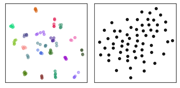
Figure 1: t-SNE embedding of datasets in (left) POC and (right) ST. POC exhibits higher task similarity; “siblings” (marked by same color) form clusters. ST contains independent datasets with no apparent clusters.

4.1.2 Testbed Setup

Meta-learning works if the new task can leverage prior knowledge; e.g., mastering motorcycle can benefit from bike riding experience. As such, MetaOD relies on the assumption that the incoming test datasets share similarity with the meta-train datasets. Otherwise, the learned knowledge from meta-train cannot be transferred to new datasets. We therefore create two testbeds with varying extent of similarity among the train/test datasets to illustrate the aforementioned point:

1. Proof-of-Concept (POC) Testbed has 100 datasets that form clusters of similar datasets. We achieve this by creating 5 different detection tasks (“siblings”) from each of the 20 “mother” datasets or mothersets.

2. Stress Testing (ST) Testbed consists of 62 independent datasets from public repositories, which exhibit lower similarity to one another.

We refer to Appendix E for the complete list of datasets and details on testbed generation. Fig. 1 illustrates the differences between POC and ST, where the meta-features of their constituting datasets are t-SNE embedded to 2-D. By construction, POC consists of clusters and hence exhibits higher task/dataset similarity as compared to ST.

4.1.3 Baselines

Being the first work for OD model selection, we do not have immediate baselines for comparison. Therefore we adapt leading methods from algorithm selection, and include additional baselines by creating variations of the proposed MetaOD (marked with $\dagger$). All the baselines can be organized into three categories:

No model selection always employs either the same single model or the ensemble of all the models:

• Local outlier factor (LOF) (Breunig et al., 2000) is a popular OD method that measures a sample’s deviation in the local region regarding its neighbors.

• Isolation Forest (iForest) (Liu et al., 2008) is a SOTA tree ensemble that measures the difficulty of “isolating” a sample via randomized splits in feature space.

• Mega Ensemble (ME) averages outlier scores from the 302 models for a given dataset. ME does not perform model selection but rather uses all the models.

Simple meta-learners pick the generally well-performing model, globally or locally:

• Global Best (GB) is the simplest meta-learner that selects the model with the largest avg. performance across all train datasets, without using meta-features.

• ISAC  (Kadioglu et al., 2010) clusters the meta-train datasets based on meta-features. Given a new dataset, it identifies its closest cluster and selects the best model with largest avg. performance on the cluster’s datasets.

• ARGOSMART (AS)  (Nikolic et al., 2013) finds the closest meta-train dataset (1NN) to a given test dataset, based on meta-feature similarity, and selects the model with the best performance on the 1NN dataset.

Optimization-based meta-learners learn meta-feature by task similarities toward optimizing performance estimates:

• Supervised Surrogates (SS) (Xu et al., 2012): Given the meta-train datasets, it directly maps the meta-features onto model performances by regression.

• ALORS (Misir & Sebag, 2017) factorizes the performance matrix to latent factors, and estimates performance as dot product of the latent factors. A non-linear regressor maps meta-features onto latent factors.

• $\dagger$MetaOD_C is a variant: performance and meta-feature matrices are concatenated as $\mathbf{C}=[\mathbf{P},\mathbf{M}]\in\mathbbm{R}^{n\times(m+d)}$, before factorization, $\mathbf{C}\approx\mathbf{U}\mathbf{V}^{T}$. Given a new dataset, zero-concatenated meta-features are projected and reconstructed as $[\widehat{\mathbf{P}}_{\text{new}};\widehat{\mathbf{M}}_{\text{new}}]=[0\ldots 0;{\mathbf{M}}_{\text{new}}]\mathbf{V}\mathbf{V}^{T}$.

• $\dagger$MetaOD_F is another variant, where $\mathbf{U}$ is fixed at $\phi(\mathbf{M})$ after the embedding step; only $\mathbf{V}$ is optimized.

In addition, we report Empirical Upper Bound (EUB) (only applicable to POC): Each POC dataset has 4 “siblings” from the same motherset with similar outlying properties. We consider the performance of the best model on a dataset’s “siblings” as its EUB, as siblings provide significant information as to which models are suitable. Given the lower task similarity in ST testbed (that is challenging for meta-learning), we include Random Selection (RS) baseline to quantify how the methods compare to random, and report the smallest $q$ that MetaOD does not significantly differ from.

4.2 POC Testbed Results

4.2.1 Testbed Setting

POC testbed is built to simulate when there are similar meta-train tasks to the test task. We use the benchmark datasets by (Emmott et al., 2016), which created “childsets” from 20 independent “mothersets” (mother datasets) by sampling. Consequently, the childsets generated from the same motherset with the same generation properties, e.g., the frequency of anomalies, are deemed to be “siblings” with large similarity. We build the POC testbed by using 5 siblings from each motherset, resulting in 100 datasets. We split them into 5 folds for cross-validation. Each test fold contains 20 independent childsets without siblings.

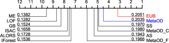
Figure 2: Comparison of avg. rank (lower is better) of methods w.r.t. performance across datasets in POC. Mean AP across datasets (higher is better) shown on lines. MetaOD is the best performing meta-learner, and comparable to EUB.

Table 1: Pairwise statistical test results between MetaOD and baselines by Wilcoxon signed rank test. Statistically better method shown in bold (both marked bold if no significance). In (left) POC, MetaOD is the only meta-learner with no difference from both EUB and the 4-$th$ best model. In (right) ST, MetaOD is the only meta-learner with no statistical difference from the 58-$th$ best model. MetaOD is statistically better than all except iForest.

Ours Baseline p-value MetaOD EUB 0.0522 MetaOD 4-th Best 0.0929 MetaOD LOF 0.0013 MetaOD iForest 0.009 MetaOD ME 0.0004 MetaOD GB 0.0051 MetaOD ISAC 0.0019 MetaOD AS 0.2959 MetaOD SS 0.7938 MetaOD ALORS 0.0025 MetaOD MetaOD_C 0.6874 MetaOD MetaOD_F 0.1165

Ours Baseline p-value MetaOD 58-th Best 0.0517 MetaOD RS 0.0001 MetaOD LOF 0.0001 MetaOD iForest 0.1129 MetaOD ME 0.0001 MetaOD GB 0.0030 MetaOD ISAC 0.0006 MetaOD AS 0.0009 MetaOD SS 0.0190 MetaOD ALORS 0.0001 MetaOD MetaOD_C 0.0001 MetaOD MetaOD_F 0.0001

4.2.2 Results

In Fig. 2, we observe that MetaOD is superior to all baseline methods w.r.t. the average rank and mean average precision (MAP), and perform comparably to the Empirical Upper Bound (EUB). Table 1 (left) shows that MetaOD is the only meta-learner that is not significantly different from both EUB (MAP=0.2051) and the 4-$th$ best model (0.2185). Moreover, MetaOD is significantly better than the baselines that do not use meta-learning (LOF (0.1282), iForest (0.1536), and ME (0.1382)), and the meta-learners including GB (0.1524), ISAC (0.1658) and ALORS (0.1728). For the full POC evaluation, see Appendix F.1.

Averaging all models (ME) does not lead to good performance as one may expect. As shown in Fig. 2, ME is the worst performing baseline by average rank in the POC testbed. Using a single detector, e.g., iForest, is significantly better. This is mainly because some models perform poorly on any given dataset, and ensembling all the models indiscriminately draws overall performance down. Using selective ensembles (Rayana & Akoglu, 2016) could be beneficial, however, ME is too expensive to use in practice. Rather a fast, low overhead meta-learner is preferable.

Meta-learners perform significantly better than methods without model selection. In particular, four meta-learners (MetaOD, SS, MetaOD_C, MetaOD_F) significantly outperform single outlier detection methods (LOF and iForest) as well as the Mega Ensemble (ME) that averages all the models. MetaOD respectively has 58.74%, 32.48%, and 47.25% higher MAP over LOF, iForest, and ME. These results signify the benefits of model selection.

Optimization-based meta learners generally perform better than simple meta learners. The top-3 meta learners by average rank (MetaOD, SS, and MetaOD_C) are all optimization-based and significantly outperform simple meta-learners like ISAC as shown in Fig. 2. Simple meta-learners weigh meta-features equally for task similarity, whereas optimization-based methods learn which meta-features matter (e.g., regression on meta-features), leading to better results. We find that MetaOD achieves 33.53%, 22.74%, and 4.73% higher MAP than simple meta-learners including GB, ISAC, and AS.

4.3 ST Testbed Results

4.3.1 Testbed Setting

When meta-train datasets lack similarity to the test dataset, it is hard to capitalize on prior experience. In the extreme case, meta-learning may not perform better than no-model-selection baselines, e.g., a single detector. To investigate the impact of the train/test similarity on meta-learning performance, we build the ST testbed that consists of 62 datasets (Appendix E Table 4) with relatively low similarity as shown in Fig. 1. For evaluation on ST, we use leave-one-out cross validation; each time using 61 datasets as meta-train.

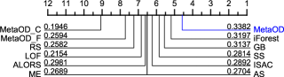
Figure 3: Comparison of avg. performance rank (lower is better) of methods across datasets in ST. Mean AP (higher is better) shown on lines. MetaOD outperforms all baselines.

4.3.2 Results

For the ST testbed, MetaOD still outperforms all baseline methods w.r.t. average rank and MAP as shown in Fig. 3. Table 1 (right) shows that MetaOD (0.3382) could select, from a pool of 302, the model that is as good as the 58-$th$ best model per dataset (0.3513). The comparable model changes from the 4-$th$ best per dataset in POC to 58-$th$ best in ST, which is expected due to the lower task similarity to leverage in ST. Notably, all other baselines are worse than the 80-$th$ best model with statistical significance. Moreover, MetaOD is significantly better than all baselines except iForest. Note that MetaOD is significantly better than RS, showing that it is able to exploit the meta-train database despite limited task similarity and not simply resorting to random picking. These results suggest that MetaOD is a good choice under various extent of similarity among train/test datasets. We refer to Appendix F.2 for detailed ST results on individual ST datasets.

Training stability affects performance for optimization-based methods. Notably, several optimization-based meta-learners, such as ALORS and MetaOD_C, do not perform well for ST. We find that the training process of matrix factorization is not stable when latent similarities are weak. In MetaOD, we employ two strategies that help stabilize the training. First, we leverage meta-feature based (rather than random) initialization. Second, we use cyclical learning rates that help escape saddle points for better local optima (Smith, 2017). Consequently, MetaOD (0.3382) significantly outperforms ALORS (0.2981) and MetaOD_C (0.1946) with 13.45% and 73.79% higher MAP.

Global methods outperform local methods under limited task similarity. In ST, datasets are less similar and simple meta-learners that leverage task similarity locally often perform poorly. For example, AS selects the model based on the 1NN, and is likely to fail if the most similar meta-train task is still quite dissimilar to the current task. On the other hand, the global meta-learner GB outperforms ISAC and AS. Note the opposite ordering among these methods in POC as shown in Fig. 2. As such, effectiveness of simple meta-learners highly depends on the train/test dataset similarity, making them harder to use in general. In contrast, MetaOD performs well in both settings.

4.4 Runtime Analysis

Fig. 4 shows that MetaOD (meta-feature generation and model selection) takes less than 1 second on most datasets, while Fig. 5 shows that it incurs only negligible overhead relative to actual training of the selected model ($\approx$10% on average). See Appendix F.3 for more comparison.

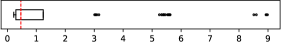
Figure 4: Boxplot of MetaOD time in POC (in sec.). MetaOD takes less than 1 sec (med. $=0.48$ shown in red) for most datasets.

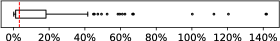
Figure 5: Boxplot of percentage of time MetaOD takes relative to the training of the selected model in POC. MetaOD incurs negligible overhead (med. $=3.3\%$ shown in red).

5 Conclusion

We introduced (to our knowledge) the first systematic model selection approach to unsupervised outlier detection (OD). The proposed MetaOD is a meta-learner, and builds on an extensive pool of historical outlier detection datasets and models. Given a new task, it selects a model based on the past performances of models on similar historical tasks. To effectively capture task similarity, we designed novel problem-specific meta-features. Importantly, MetaOD is ($i$) fully unsupervised, requiring no model evaluations at test time, and ($ii$) lightweight, incurring relatively small selection time overhead prior to model estimation. Extensive experiments on two large testbeds showed that MetaOD significantly improves detection performance over directly using some of the most popular models as well as several state-of-the-art unsupervised meta-learners.

We open-source MetaOD for future deployment. We expect meta-learning to get more powerful as the meta-train database grows. Therefore, we also share all our code and testbeds for the community to contribute new datasets and models to stimulate further advances on automating OD.

Supplementary Material: Automating Outlier Detection via Meta-Learning

Details on Models, Meta-features, Datasets/Testbeds, Optimization, and Detailed Experiment Result

Appendix A MetaOD Model Set

Model set $\mathbcal{M}$ is composed by pairing outlier detection algorithms to distinct hyperparameter choices. Table 2 provides a comprehensive description of models, including 302 unique models composed by 8 popular outlier detection (OD) algorithms. All models and parameters are based on the Python Outlier Detection Toolbox (PyOD).

Table 2: Outlier Detection Models; see hyperparameter definitions from PyOD (Zhao et al., 2019)

Detection algorithm	Hyperparameter 1	Hyperparameter 2	Total
LOF (Breunig et al., 2000)	n_neighbors: $[1,5,10,15,20,25,50,60,70,80,90,100]$	distance: [’manhattan’, ’euclidean’, ’minkowski’]	36
kNN (Ramaswamy et al., 2000)	n_neighbors: $[1,5,10,15,20,25,50,60,70,80,90,100]$	method: [’largest’, ’mean’, ’median’]	36
OCSVM (Schölkopf et al., 2001)	nu (train error tol): $[0.1,0.2,0.3,0.4,0.5,0.6,0.7,0.8,0.9]$	kernel: [’linear’, ’poly’, ’rbf’, ’sigmoid’]	36
COF (Tang et al., 2002)	n_neighbors: $[3,5,10,15,20,25,50]$	N/A	7
ABOD (Kriegel et al., 2008)	n_neighbors: $[3,5,10,15,20,25,50,60,70,80,90,100]$	N/A	7
iForest (Liu et al., 2008)	n_estimators: $[10,20,30,40,50,75,100,150,200]$	max_features: $[0.1,0.2,0.3,0.4,0.5,0.6,0.7,0.8,0.9]$	81
HBOS (Goldstein & Dengel, 2012)	n_histograms: $[5,10,20,30,40,50,75,100]$	tolerance: $[0.1,0.2,0.3,0.4,0.5]$	40
LODA (Pevný, 2016)	n_bins: $[10,20,30,40,50,75,100,150,200]$	n_random_cuts: $[5,10,15,20,25,30]$	54
			302

Appendix B OD Meta-Features

B.1 Complete List of Features

We summarize the meta-features used by MetaOD in Table 3. When applicable, we provide the formula for computing the meta-feature(s) and corresponding variants. Some are based on (Vanschoren, 2018). Refer to the accompanied code for details.

Specifically, meta-features can be categorized into (1) statistical features, and (2) landmarker features. Broadly speaking, the former captures statistical properties of the underlying data distributions; e.g., min, max, variance, skewness, covariance, etc. of the features and feature combinations. These statistics-based meta-features have been commonly used in the AutoML literature (Vanschoren, 2018).

Table 3: Selected meta-features for characterizing an arbitrary dataset. See code for details.

Name	Formula	Rationale	Variants
Nr instances	n	Speed, Scalability	$\frac{p}{n}$, $\log(n)$, $\log(\frac{n}{p})$
Nr features	p	Curse of dimensionality	$\log(p)$, % categorical
Sample mean	$\mu$	Concentration
Sample median	$\tilde{X}$	Concentration
Sample var	$\sigma^{2}$	Dispersion
Sample min	$\max_{X}$	Data range
Sample max	$\min_{X}$	Data range
Sample std	$\sigma$	Dispersion
Percentile	$P_{i}$	Dispersion	q1, q25, q75, q99
Interquartile Range (IQR)	$q75-q25$	Dispersion
Normalized mean	$\frac{\mu}{\max_{X}}$	Data range
Normalized median	$\frac{\tilde{X}}{\max_{X}}$	Data range
Sample range	$\max_{X}-\min_{X}$	Data range
Sample Gini		Dispersion
Median absolute deviation	$\text{median}(X-\tilde{X})$	Variability and dispersion
Average absolute deviation	$\text{avg}(X-\tilde{X})$	Variability and dispersion
Quantile Coefficient Dispersion	$\frac{(q75-q25)}{(q75+q25)}$	Dispersion
Coefficient of variance		Dispersion
Outlier outside 1 & 99	% samples outside 1% or 99%	Basic outlying patterns
Outlier 3 STD	% samples outside $3\sigma$	Basic outlying patterns
Normal test	If a sample differs from a normal dist.	Feature normality
$k$th moments			5th to 10th moments
Skewness	Feature skewness	Feature normality	$\min$, $\max$, $\mu$, $\sigma$, skewness, kurtosis
Kurtosis	$\frac{\mu_{4}}{\sigma^{4}}$	Feature normality	$\min$, $\max$, $\mu$, $\sigma$, skewness, kurtosis
Correlation	$\rho$	Feature interdependence	$\min$, $\max$, $\mu$, $\sigma$, skewness, kurtosis
Covariance	Cov	Feature interdependence	$\min$, $\max$, $\mu$, $\sigma$, skewness, kurtosis
Sparsity	$\frac{\#\text{Unique values}}{n}$	Degree of discreteness	$\min$, $\max$, $\mu$, $\sigma$, skewness, kurtosis
ANOVA p-value	$p_{\text{ANOVA}}$	Feature redundancy	$\min$, $\max$, $\mu$, $\sigma$, skewness, kurtosis
Coeff of variation	$\frac{\sigma_{x}}{\mu_{x}}$	Dispersion
Norm. entropy	$\frac{H(X)}{log_{2}n}$	Feature informativeness	min,max, $\sigma$, $\mu$
Landmarker (HBOS)	See §B.2	Outlying patterns	Histogram density
Landmarker (LODA)	See §B.2	Outlying patterns	Histogram density
Landmarker (PCA)	See §B.2	Outlying patterns	Explained variance ratio, singular values
Landmarker (iForest)	See §B.2	Outlying patterns	# of leaves, tree depth, feature importance

B.2 Landmarker Meta-Feature Generation

In addition to statistical meta-features, we use four OD-specific landmarker algorithms for computing OD-specific landmarker meta-features, iForest (Liu et al., 2008), HBOS (Goldstein & Dengel, 2012), LODA (Pevný, 2016), and PCA (Idé & Kashima, 2004) (reconstruction error as outlier score), to capture outlying characteristics of a dataset. To this end, we first provide a quick overview of each algorithm and then discuss how we are using them for building meta-features. The algorithms are executed with the default parameter. Refer to the attached code for details of meta-feature construction.

Isolation Forest (iForest) (Liu et al., 2008) is a tree-based ensemble method. Specifically, iForest builds a collection of base trees using the subsampled unlabeled data, splitting on (randomly selected) features as nodes. iForest grows internal nodes until the terminal leaves contain only one sample or the predefined max depth is reached. Given the max depth is not set and we have multiple base trees with each leaf containing one sample only, the anomaly score of a sample is the aggregated depth the leaves the sample falls into. The key assumption is that an anomaly is more different than the normal samples, and is, therefore, easier to be “isolated” during the node splitting. Consequently, anomalies are closer to roots with small tree depth. For iForest, we use the balance of base trees (i.e., depth of trees and number of leaves per tree) and additional information (e.g., feature importance of each base tree). It is noted that feature importance information is available for each base tree—we therefore analyze the statistic of mean and max of base tree feature importance. Specifically, the following information of base trees are used:

• Tree depth: min, max, mean, std, skewness, and kurtosis

• Number of leaves: min, max, mean, std, skewness, and kurtosis

• Mean of base tree feature importance: min, max, mean, std, skewness, and kurtosis

• Max of base tree feature importance: min, max, mean, std, skewness, and kurtosis

Histogram-based Outlier Scores (HBOS) (Goldstein & Dengel, 2012) assumes that each dimension (feature) of the datasets is independent. It builds a histogram on each feature to calculate the density. Given there are $n$ samples and $d$ features, for each histogram from $1...d$, HBOS estimates the sample density using all $n$ samples. Intuitively, the anomaly score of sample $g$ is defined as the sum of log of inverse density. In other words, it can be considered as an aggregation of density estimation on each feature. Obviously, the samples falling in high-density areas are more likely to be normal points and vice versa. The following information is included as part of MetaOD:

• Mean of each histogram (per feature): min, max, mean, std, skewness, and kurtosis

• Max of each histogram (per feature) : min, max, mean, std, skewness, and kurtosis

Lightweight on-line detector of anomalies (LODA) (Pevný, 2016) is a fast ensemble-based anomaly detection algorithm. It shares a similar idea as HBOS—“although one one-dimensional histogram is a very weak anomaly detector, their collection yields to a strong detector”. Different from HBOS that simply aggregates over all independent histograms, LODA extends the histogram-based model generating $k$ random projection vectors to compress data into one-dimensional space for building histograms. Similar to HBOS, we include in the following information as part of meta-features:

• Mean of each random projection (per feature): min, max, mean, std, skewness, and kurtosis

• Max of each random projection (per feature) : min, max, mean, std, skewness, and kurtosis

• Mean of each histogram (per feature): min, max, mean, std, skewness, and kurtosis

• Max of each histogram (per feature) : min, max, mean, std, skewness, and kurtosis

Principal component analysis based outlier detector (PCA) (Idé & Kashima, 2004) aims to quantify sample outlyingness by projecting them into lower dimensions through principal component analysis. Since the number of normal samples is much bigger than the number of outliers, the identified projection matrix is mainly suited for normal samples. Consequently, the reconstruction error of normal samples are smaller than that of outlier samples, which can be used to measure sample outlyingness. For PCA, we include the following information into meta-features:

• Explained variance ratio on the first three principal components: The percentage of variance it captures for the top 3 principal components

• Singular values: The top 3 singular values generated during SVD process

Additionally, we also leverage the outlier scores by OD landmarkers after appropriate scaling, e.g., normalization/standardization.

Appendix C Gradient Derivations

In this section we provide the details for the gradient derivation of MetaOD. It is organized as follow. We first provide a quick overview of gradient derivation in classical recommender systems, and then show the derivation of the rank-based criterion used in MetaOD.

C.1 Background

Given a rating matrix $\mathbf{P}\in\mathbb{R}^{n\times m}$ with $n$ users rating on $m$ items, $\mathbf{P}_{ij}$ denotes $i$th user’s rating on the $j$th item in classical recommender system setting. For learning the latent factors in $k$ dimensions, we try to factorize $\mathbf{P}$ into user matrix $\mathbf{U}\in\mathbb{R}^{n\times k}$ and the item matrix $\mathbf{V}\in\mathbb{R}^{d\times k}$ to make $\mathbf{P}\approx\mathbf{U}\mathbf{V}^{T}$.

In classical matrix factorization setting, some entries of the performance matrix $\mathbf{P}$ is missing. Consequently, one may use stochastic gradient descent to minimize the mean squared error (MSE) between $\mathbf{P}$ and $\mathbf{U}\mathbf{V}^{T}$ through all non-empty entries. For each rating $\mathbf{P}_{ij}$, the loss $L$ is defined as:

$$L_{i,j}=L(\mathbf{U}_{i},\mathbf{V}^{T}_{j})=(\mathbf{P}_{ij}-\mathbf{U}_{i}\mathbf{V}^{T}_{j})^{2}$$ (9)

The total loss over all non-empty entries is:

$$L=\sum_{i,j}(\mathbf{P}_{ij}-\mathbf{U}_{i}\mathbf{V}^{T}_{j})^{2}$$ (10)

The optimization process iterates over all non-empty entries of the performance matrix $\mathbf{P}$, and updates $\mathbf{U}_{i}$ and $\mathbf{V}_{j}$ using the learning rate $\eta$ as:

$$\mathbf{U}_{i}\leftarrow\mathbf{U}_{i}-\eta\frac{\partial L}{\partial\mathbf{U}_{i}}$$ (11)

$$\mathbf{V}_{j}\leftarrow\mathbf{V}_{j}-\eta\frac{\partial L}{\partial\mathbf{V}_{j}}$$ (12)

C.2 Rank-based Criterion

For unsupervised OD model selection, a rank-based criteria is preferable since we are concerned most with the order of model performance other than absolute value, especially the top-1 ranked model. We therefore choose the negative form of discounted cumulative gain (DCG) as the objective function for dataset-wise optimization, which is defined as:

$$\text{DCG}=\sum_{r}\frac{b^{rel_{r}}-1}{\log_{2}(r+1)}$$ (13)

where $rel_{r}$ depicts the relevance of the item ranked at the $r$th position and $b$ is a scalar (typically set to 2). In our setting, we use the performance of a model to reflect its relevance to a dataset. As such, DCG for dataset $i$ is re-written as

$$\text{DCG}_{i} =\sum_{j=1}^{m}\frac{b^{{\mathbf{P}_{ij}}}-1}{\log_{2}(1+\sum_{k=1}^{m}\mathbbm{1}{[\widehat{\mathbf{P}}_{ij}\leq\widehat{\mathbf{P}}_{ik}}])}$$ (14)

where $\widehat{\mathbf{P}}_{ij}=\langle\mathbf{U}_{i},\mathbf{V}_{j}\rangle$ is the predicted performance. Intuitively, ranking high-performing models at the top leads to higher DCG, and a larger $b$ increases the emphasis on the quality at higher rank positions.

A challenge with DCG is that it is not differentiable as it involves ranking/sorting. Specifically, the sum term in the denominator of Eq. (14) uses (nonsmooth) indicator functions to obtain the position of model $j$ as ranked by the estimated performances. We circumvent this challenge by replacing the indicator function by the (smooth) sigmoid approximation (Fréry et al., 2017) shown in Eq. (15).

$$\mathbbm{1}{[\widehat{\mathbf{P}}_{ij}\leq\widehat{\mathbf{P}}_{ik}}]\approx\frac{1}{1+\exp(-\alpha(\widehat{\mathbf{P}}_{ik}-\widehat{\mathbf{P}}_{ij}))}=\sigma(\widehat{\mathbf{P}}_{ik}-\widehat{\mathbf{P}}_{ij})$$ (15)

The approximated DCG criterion for the $i$th dataset is:

$$\text{DCG}_{i}\approx\text{sDCG}_{i}=\small{\sum_{j=1}^{m}\frac{b^{{\mathbf{P}_{ij}}}-1}{\log_{2}(1+\sum_{k=1}^{m}\sigma(\widehat{\mathbf{P}}_{ik}-\widehat{\mathbf{P}}_{ij}))}}$$ (16)

Consequently, we optimize the smoothed loss:

$$L=-\sum_{i}^{n}\text{sDCG}_{i}(\mathbf{P}_{i},\mathbf{U}_{i}\mathbf{V}^{T})$$ (17)

which can be rewritten as:

$$\min_{\mathbf{U},\mathbf{V}}\;\;-\sum_{i=1}^{n}\text{DCG}_{i}(\mathbf{P}_{i},\mathbf{U}_{i}\mathbf{V}^{T})\;.$$ (18)

C.3 Gradient Derivation for DCG based Criterion

As we aim to maximize the total dataset-wise DCG, we make a pass over meta-train datasets one by one at each epoch as shown in Algorithm 1. We update $\mathbf{U}_{i}$ and $\mathbf{V}_{j}$ by gradient descent as shown below. It is noted that predicted performance of $j$th model on $i$th dataset is defined as the dot product of corresponding dataset and model vector: $\widehat{\mathbf{P}}_{ij}=\mathbf{U}_{i}\mathbf{V}^{T}_{j}$. So Eq. (16) can be rearranged as:

$$-\text{DCG}_{i} =\sum_{j=1}^{m}\frac{b^{{\mathbf{P}_{ij}}}-1}{\log_{2}(1+\sum_{k=1}^{m}\sigma(\widehat{\mathbf{P}}_{ik}-\widehat{\mathbf{P}}_{ij}))}$$

$$=\ln(2)\sum_{j=1}^{m}\frac{b^{{\mathbf{P}_{ij}}}-1}{\ln(1+\sum_{k=1}^{m}\sigma(\mathbf{U}_{i}\mathbf{V}^{T}_{k}-\mathbf{U}_{i}\mathbf{V}^{T}_{j}))}$$

$$=\ln(2)\sum_{j=1}^{m}\frac{b^{{\mathbf{P}_{ij}}}-1}{\ln(1+\sigma(0)+\sum_{k\neq j}\sigma(\mathbf{U}_{i}\mathbf{V}^{T}_{k}-\mathbf{U}_{i}\mathbf{V}^{T}_{j}))}$$

$$=\ln(2)\sum_{j=1}^{m}\frac{b^{{\mathbf{P}_{ij}}}-1}{\ln(\frac{3}{2}+\sum_{k\neq j}\sigma(\mathbf{U}_{i}\mathbf{V}^{T}_{k}-\mathbf{U}_{i}\mathbf{V}^{T}_{j}))}$$

$$=\ln(2)\sum_{j=1}^{m}\frac{b^{{\mathbf{P}_{ij}}}-1}{\ln(\frac{3}{2}+\sum_{k\neq j}\sigma(\mathbf{U}_{i}\mathbf{V}^{T}_{k}-\mathbf{U}_{i}\mathbf{V}^{T}_{j}))}$$

We compute the gradient of $\mathbf{U}_{i}$ and $\mathbf{V}^{T}_{j}$ as the partial derivative of $-\text{DCG}_{i}$ as shown in Eq. (C.3). To ease the notation, we define:

$$w^{i}_{jk}=\mathbf{U}_{i}\mathbf{V}^{T}_{k}-\mathbf{U}_{i}\mathbf{V}^{T}_{j}=\langle\mathbf{U}_{i},(\mathbf{V}_{k}-\mathbf{V}_{j})\rangle$$ (20)

$$\beta^{i}_{j} =\frac{3}{2}+\sum_{k\neq j}\sigma(\mathbf{U}_{i}\mathbf{V}^{T}_{k}-\mathbf{U}_{i}\mathbf{V}^{T}_{j})$$

$$=\frac{3}{2}+\sum_{k\neq j}\sigma(w^{i}_{jk})$$ (21)

By plugging Eq. (20) and (C.3) back into Eq. (C.3), it is simplified into:

$$-\text{DCG}_{i} =\ln(2)\sum_{j=1}^{m}\frac{b^{{\mathbf{P}_{ij}}}-1}{\ln(\frac{3}{2}+\sum_{k\neq j}\sigma(\mathbf{U}_{i}\mathbf{V}^{T}_{k}-\mathbf{U}_{i}\mathbf{V}^{T}_{j}))}$$

$$=\ln(2)\sum_{j=1}^{m}\frac{b^{{\mathbf{P}_{ij}}}-1}{\ln(\beta^{i}_{j})}$$

We then obtain the gradients of $\mathbf{U}_{i}$ and $\mathbf{V}^{T}_{j}$ as follows:

$$\frac{\partial L}{\partial\mathbf{U}_{i}} =\frac{\partial(-\text{DCG}_{i})}{\partial\mathbf{U}_{i}}$$

$$=\ln(2)\frac{\partial\left(\sum_{j=1}^{m}\frac{b^{{\mathbf{P}_{ij}}}-1}{\ln(\beta^{i}_{j})}\right)}{\partial\mathbf{U}_{i}}$$

$$=\ln{(2)}\sum_{j=1}^{m}\left[\frac{b^{\mathbf{P}_{ij}}-1}{\beta^{i}_{j}\ln^{2}{(\beta^{i}_{j})}}\sum_{k\neq j}\sigma(w^{i}_{jk})(1-\sigma(w^{i}_{jk}))(\mathbf{V}_{k}-\mathbf{V}_{j})\right]$$ (23)

$$\frac{\partial L}{\partial\mathbf{V}_{j}} =\frac{\partial(-\text{DCG}_{i})}{\partial\mathbf{V}_{j}}$$

$$=\ln(2)\frac{\partial\left(\sum_{j=1}^{m}\frac{b^{{\mathbf{P}_{ij}}}-1}{\ln(\beta^{i}_{j})}\right)}{\partial\mathbf{U}_{i}}$$

$$=-\ln{(2)}\sum_{j=1}^{m}\left[\frac{b^{\mathbf{P}_{ij}}-1}{\beta^{i}_{j}\ln^{2}{(\beta^{i}_{j})}}{\sum_{k\neq j}\sigma(w^{i}_{jk})(1-\sigma(w^{i}_{jk}))\mathbf{U}_{i}}\right]$$ (24)

Appendix D MetaOD Flowchart

Fig. 6 shows the major components of MetaOD. We highlight the components transferred from offline to online stage (model selection) in blue; namely, meta-feature extractors ($\psi$), embedding model ($\phi$), regressor $f$, model matrix $\mathbf{U}$, and dataset matrix $\mathbf{V}$.

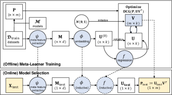
Figure 6: MetaOD overview; components that transfer from offline to online (model selection) phase shown in blue.

Appendix E Dataset Description and Testbed Setup

E.1 POC Testbed Setup

POC testbed is built to simulate the testbed when meta-train and test datasets come from similar distribution. Model selection on test data can therefore benefit from the prior experience on the train set. For this purpose, we use the benchmark datasets (Emmott et al., 2016). In short, they adapt 19 datasets from UCI repository and also create a synthetic dataset to make a pool of 20 “mothersets”. For each motherset, they first separate anomalies from normal points, and then generate “childsets” from the motherset by sampling and controlling outlying properties: (i) point difficulty; (ii) relative frequency, i.e., the number of anomalies; (iii) clusteredness and (iv) feature irrelevance. Taking this approach, the childsets generated from the same motherset with the same properties are deemed to be “siblings” with high similarity. Refer to the original paper for details of the data generation process.

We build the POC testbed by selecting five siblings from each motherset, resulting in 100 datasets. For robustness, we split the 100 datasets into 5 folds for cross-validation. Each fold contains 20 independent datasets with no siblings, and the corresponding train set (80 datasets) contain their siblings. Refer to the code for the 100 randomly selected childsets for POC testbed.

E.2 ST Testbed Setup

Different from the setting of POC, ST testbed aims to test out MetaOD’s performance when the meta-learning assumption does not hold: train and test datasets are all independent with limited similarity.

To build the ST testbed, we combine the datasets from three different sources resulting in 62 independent datasets as shown in Table 4: (i) 23 datasets from ODDS Library ; (ii) 19 datasets DAMI datasets (Campos et al., 2016) as well as (iii) 20 benchmark datasets (Emmott et al., 2016) used in POC. For ST testbed, we run leave-one-out cross validation. So each time 61 datasets are used for meta-train and the remaining one for test.

Table 4: ST testbed composed by ODDS library (23 datasets), DAMI library (19 datasets), and Emmott benchmark (20 datasets)

	Data	Pts	Dim	% Outlier
1	annthyroid (ODDS)	7200	6	7.4167
2	arrhythmia (ODDS)	452	274	14.6018
3	breastw (ODDS)	683	9	34.9927
4	glass (ODDS)	214	9	4.2056
5	ionosphere (ODDS)	351	33	35.8974
6	letter (ODDS)	1600	32	6.25
7	lympho (ODDS)	148	18	4.0541
8	mammography (ODDS)	11183	6	2.325
9	mnist (ODDS)	7603	100	9.2069
10	musk (ODDS)	3062	166	3.1679
11	optdigits (ODDS)	5216	64	2.8758
12	pendigits (ODDS)	6870	16	2.2707
13	pima (ODDS)	768	8	34.8958
14	satellite (ODDS)	6435	36	31.6395
15	satimage-2 (ODDS)	5803	36	1.2235
16	shuttle (ODDS)	49097	9	7.1511
17	smtp_n (ODDS)	95156	3	0.0315
18	speech (ODDS)	3686	400	1.6549
19	thyroid (ODDS)	3772	6	2.4655
20	vertebral (ODDS)	240	6	12.5
21	vowels (ODDS)	1456	12	3.4341
22	wbc (ODDS)	378	30	5.5556
23	wine (ODDS)	129	13	7.7519
24	Annthyroid (DAMI)	7129	21	7.4905
25	Arrhythmia (DAMI)	450	259	45.7778
26	Cardiotocography (DAMI)	2114	21	22.0435
27	HeartDisease (DAMI)	270	13	44.4444
28	Hepatitis (DAMI)	80	19	16.25
29	InternetAds (DAMI)	1966	1555	18.7182
30	PageBlocks (DAMI)	5393	10	9.4567
31	Pima (DAMI)	768	8	34.8958
32	SpamBase (DAMI)	4207	57	39.9097
33	Stamps (DAMI)	340	9	9.1176
34	Wilt (DAMI)	4819	5	5.3331
35	ALOI (DAMI)	49534	27	3.0444
36	Glass (DAMI)	214	7	4.2056
37	PenDigits (DAMI)	9868	16	0.2027
38	Shuttle (DAMI)	1013	9	1.2833
39	Waveform (DAMI)	3443	21	2.9044
40	WBC (DAMI)	223	9	4.4843
41	WDBC (DAMI)	367	30	2.7248
42	WPBC (DAMI)	198	33	23.7374
43	abalone_1231 (Emmott)	1986	15	5.0352
44	comm.and.crime_0936 (Emmott)	910	404	1.0989
45	concrete_1096 (Emmott)	468	32	1.0684
46	fault_0246 (Emmott)	278	38	17.9856
47	gas_0321 (Emmott)	6000	128	0.1
48	imgseg_1526 (Emmott)	1320	25	10
49	landsat_1761 (Emmott)	230	36	10
50	letter.rec_1666 (Emmott)	4089	23	10.0024
51	magic.gamma_1411 (Emmott)	6000	22	5
52	opt.digits_1316 (Emmott)	3180	248	5
53	pageb_0126 (Emmott)	733	14	16.2347
54	particle_1336 (Emmott)	6000	200	5
55	shuttle_0071 (Emmott)	6000	20	16.3167
56	skin_1706 (Emmott)	6000	4	10
57	spambase_0681 (Emmott)	2522	57	0.5155
58	synthetic_1786 (Emmott)	329	14	10.0304
59	wave_0661 (Emmott)	3024	21	0.5291
60	wine_0611 (Emmott)	3720	24	0.5108
61	yeast_1221 (Emmott)	926	8	5.0756
62	yearp_0231 (Emmott)	6000	202	48.6

Appendix F Additional Experiment Results

F.1 Experiment Results for POC Testbed

We present the performances of compared methods in Table 5, and hypothesis test results in Table 6. It is noted these results are averaged across five folds. The results shows that MetaOD achieves the best MAP among all meta-learners.

Table 5: Method evaluation in POC testbed (average precision). The most performing method is highlighted in bold. The rank is provided in parenthesis (lower ranks denote better performance). MetaOD achieves the best average precision and average rank among all meta-learners.

. Dataset LOF iForest ME GB ISAC AS SS ALORS MetaOD_C MetaOD_F MetaOD EUB abalone 0.0812 (12) 0.1679 (10) 0.1441 (11) 0.1738 (9) 0.192 (6) 0.229 (3) 0.224 (4) 0.1747 (8) 0.1815 (7) 0.2141 (5) 0.2329 (2) 0.2394 (1) comm.and.crime 0.0839 (10) 0.0913 (8) 0.0797 (11) 0.0855 (9) 0.0638 (12) 0.1001 (5) 0.1122 (2) 0.099 (7) 0.1079 (3) 0.0999 (6) 0.1072 (4) 0.1156 (1) concrete 0.0297 (2) 0.0279 (3) 0.0298 (1) 0.0251 (5) 0.0224 (7) 0.022 (8) 0.0279 (3) 0.0236 (6) 0.0131 (12) 0.0198 (9) 0.0185 (10) 0.0147 (11) fault 0.1898 (12) 0.3755 (7) 0.323 (10) 0.3735 (8) 0.197 (11) 0.3949 (2) 0.3778 (5) 0.3723 (9) 0.4217 (1) 0.3813 (4) 0.3768 (6) 0.3899 (3) gas 0.0193 (5) 0.0031 (11) 0.0083 (8) 0.0033 (10) 0.0059 (9) 0.0481 (1) 0.0152 (6) 0.0024 (12) 0.0392 (2) 0.013 (7) 0.0229 (4) 0.0387 (3) imgseg 0.1153 (12) 0.3618 (6) 0.2586 (11) 0.3598 (9) 0.3659 (5) 0.3514 (10) 0.3891 (4) 0.3605 (8) 0.3612 (7) 0.3989 (3) 0.408 (2) 0.4166 (1) landsat 0.1644 (4) 0.1306 (9) 0.131 (8) 0.13 (10) 0.1071 (12) 0.1578 (5) 0.138 (7) 0.1111 (11) 0.1844 (1) 0.1562 (6) 0.1784 (3) 0.1844 (1) letter.rec 0.1529 (7) 0.0986 (11) 0.112 (9) 0.0991 (10) 0.0946 (12) 0.222 (2) 0.218 (5) 0.1168 (8) 0.2216 (3) 0.2229 (1) 0.2179 (6) 0.2216 (3) magic.gamma 0.1152 (9) 0.1303 (4) 0.1104 (10) 0.1314 (3) 0.1096 (11) 0.1319 (2) 0.1299 (5) 0.1294 (6) 0.102 (12) 0.1255 (8) 0.1263 (7) 0.1351 (1) opt.digits 0.0662 (9) 0.0668 (7) 0.0603 (12) 0.0665 (8) 0.0742 (3) 0.0795 (2) 0.0689 (6) 0.0606 (11) 0.0705 (4) 0.066 (10) 0.0701 (5) 0.0803 (1) pageb 0.3956 (11) 0.4581 (6) 0.3801 (12) 0.4574 (7) 0.4384 (9) 0.4829 (3) 0.4616 (5) 0.4621 (4) 0.4281 (10) 0.4498 (8) 0.4898 (2) 0.4939 (1) particle 0.0546 (12) 0.0782 (5) 0.0626 (11) 0.0746 (8) 0.0761 (6) 0.1 (1) 0.0936 (3) 0.0739 (9) 0.0683 (10) 0.0867 (4) 0.0757 (7) 0.0982 (2) shuttle 0.2015 (11) 0.2058 (9) 0.1935 (12) 0.2056 (10) 0.2961 (5) 0.3165 (3) 0.2711 (7) 0.2105 (8) 0.3165 (3) 0.2932 (6) 0.3225 (1) 0.3185 (2) skin 0.1161 (9) 0.0926 (11) 0.0995 (10) 0.0911 (12) 0.1814 (6) 0.165 (8) 0.2408 (4) 0.1737 (7) 0.2808 (1) 0.2808 (1) 0.2808 (1) 0.2278 (5) spambase 0.0187 (12) 0.0713 (9) 0.0571 (11) 0.0706 (10) 0.0873 (6) 0.0744 (8) 0.1292 (1) 0.0757 (7) 0.0981 (4) 0.112 (2) 0.0942 (5) 0.0982 (3) synthetic 0.1233 (4) 0.1226 (5) 0.1157 (8) 0.1132 (11) 0.154 (1) 0.1218 (6) 0.1147 (10) 0.1151 (9) 0.1468 (3) 0.1182 (7) 0.1483 (2) 0.1046 (12) wave 0.0577 (9) 0.0114 (12) 0.0297 (10) 0.0117 (11) 0.2925 (8) 0.3413 (5) 0.3486 (1) 0.3244 (7) 0.3486 (1) 0.344 (4) 0.3365 (6) 0.3486 (1) wine 0.0082 (11) 0.0087 (5) 0.0084 (10) 0.0085 (8) 0.0085 (8) 0.0073 (12) 0.0087 (5) 0.0124 (2) 0.0097 (3) 0.0086 (7) 0.0088 (4) 0.0129 (1) yeast 0.0813 (2) 0.0781 (4) 0.073 (8) 0.0762 (6) 0.0796 (3) 0.068 (11) 0.0781 (4) 0.0693 (9) 0.0885 (1) 0.067 (12) 0.0733 (7) 0.0688 (10) yearp 0.4894 (5) 0.4911 (4) 0.4862 (7) 0.4913 (3) 0.4703 (12) 0.4716 (10) 0.4916 (2) 0.4891 (6) 0.4716 (10) 0.4741 (9) 0.4801 (8) 0.4937 (1) average 0.1282 (8.7) 0.1536 (7.4) 0.1382 (9.7) 0.1524 (8.35) 0.1658 (7.6) 0.1943 (5.49) 0.197 (4.95) 0.1728 (7.6) 0.198 (4.9) 0.1966 (5.95) 0.2035 (4.48) 0.2051 (3.2) STD 0.1219 0.1487 0.1294 0.1489 0.1386 0.1491 0.1486 0.1487 0.1485 0.1530 0.1587 0.156

Table 6: Pairwise statistical test results between MetaOD and baselines by Wilcoxon signed rank test in POC. Statistically better method shown in bold (both marked bold if no significance). MetaOD related pairs are surrounded by rectangles. MetaOD (MAP=0.2035) is statistically significantly better than baselines including LOF (0.1282), iForest (0.1536), ME (0.1382), GB (0.1524), ISAC (0.1658), and ALORS (0.1728), and comparable to EUB (0.2051), the empirical upper bound.

Method 1 Method 2 p-value LOF (0.1282) IForest (0.1536) 0.3135 LOF (0.1282) ME (0.1382) 0.433 LOF (0.1282) GB (0.1524) 0.4553 LOF (0.1282) ISAC (0.1658) 0.1005 LOF (0.1282) AS (0.1943) 0.0025 LOF (0.1282) SS (0.197) 0.0045 LOF (0.1282) ALORS (0.1728) 0.062 LOF (0.1282) MetaOD_C (0.198) 0.001 LOF (0.1282) MetaOD_F (0.1966) 0.01 LOF (0.1282) MetaOD (0.2035) 0.0013 LOF (0.1282) EUB (0.2051) 0.0007 IForest (0.1536) ME (0.1382) 0.029 IForest (0.1536) GB (0.1524) 0.0365 IForest (0.1536) ISAC (0.1658) 0.7369 IForest (0.1536) AS (0.1943) 0.008 IForest (0.1536) SS (0.197) 0.0012 IForest (0.1536) ALORS (0.1728) 0.6274 IForest (0.1536) MetaOD_C (0.198) 0.0276 IForest (0.1536) MetaOD_F (0.1966) 0.0276 IForest (0.1536) MetaOD (0.2035) 0.009 IForest (0.1536) EUB (0.2051) 0.001 ME (0.1382) GB (0.1524) 0.0569

Method 1 Method 2 p-value ME (0.1382) ISAC (0.1658) 0.156 ME (0.1382) AS (0.1943) 0.0005 ME (0.1382) SS (0.197) 0.0002 ME (0.1382) ALORS (0.1728) 0.009 ME (0.1382) MetaOD_C (0.198) 0.0008 ME (0.1382) MetaOD_F (0.1966) 0.0012 ME (0.1382) MetaOD (0.2035) 0.0004 ME (0.1382) EUB (0.2051) 0.0004 GB (0.1524) ISAC (0.1658) 0.7172 GB (0.1524) AS (0.1943) 0.0032 GB (0.1524) SS (0.197) 0.0002 GB (0.1524) ALORS (0.1728) 0.3703 GB (0.1524) MetaOD_C (0.198) 0.0169 GB (0.1524) MetaOD_F (0.1966) 0.0111 GB (0.1524) MetaOD (0.2035) 0.0051 GB (0.1524) EUB (0.2051) 0.0008 ISAC (0.1658) AS (0.1943) 0.0169 ISAC (0.1658) SS (0.197) 0.0051 ISAC (0.1658) ALORS (0.1728) 0.6542 ISAC (0.1658) MetaOD_C (0.198) 0.062 ISAC (0.1658) MetaOD_F (0.1966) 0.008 ISAC (0.1658) MetaOD (0.2035) 0.0019

Method 1 Method 2 p-value ISAC (0.1658) EUB (0.2051) 0.0015 AS (0.1943) SS (0.197) 0.9702 AS (0.1943) ALORS (0.1728) 0.0206 AS (0.1943) MetaOD_C (0.198) 0.8446 AS (0.1943) MetaOD_F (0.1966) 0.3135 AS (0.1943) MetaOD (0.2035) 0.2959 AS (0.1943) EUB (0.2051) 0.0304 SS (0.197) ALORS (0.1728) 0.0003 SS (0.197) MetaOD_C (0.198) 0.8092 SS (0.197) MetaOD_F (0.1966) 0.4553 SS (0.197) MetaOD (0.2035) 0.7938 SS (0.197) EUB (0.2051) 0.099 ALORS (0.1728) MetaOD_C (0.198) 0.0276 ALORS (0.1728) MetaOD_F (0.1966) 0.0137 ALORS (0.1728) MetaOD (0.2035) 0.0025 ALORS (0.1728) EUB (0.2051) 0.0006 MetaOD_C (0.198) MetaOD_F (0.1966) 0.7475 MetaOD_C (0.198) MetaOD (0.2035) 0.6874 MetaOD_C (0.198) EUB (0.2051) 0.1773 MetaOD_F (0.1966) MetaOD (0.2035) 0.1165 MetaOD_F (0.1966) EUB (0.2051) 0.0251 MetaOD (0.2035) EUB (0.2051) 0.0522

F.2 Experiment Results for ST Testbed

We present the method performance in Table 7, and hypothesis test result in Table 8. Among all meta-learners, MetaOD shows the best MAP.

Table 7: Method evaluation in ST testbed (average precision). The most performing method is highlighted in bold. The rank is provided in parenthesis (lower ranks denote better performance). MetaOD achieves the best average precision and average rank among all meta-learners.

Datasets	LOF	iForest	ME	GB	ISAC	AS	SS	ALORS	MetaOD_c	MetaOD_F	RS	MetaOD
abalone	0.092 (10)	0.1654 (2)	0.1338 (6)	0.1584 (3)	0.15 (4)	0.1232 (9)	0.1688 (1)	0.1316 (7)	0.0737 (12)	0.1274 (8)	0.092 (10)	0.1355 (5)
ALOI	0.1424 (2)	0.0333 (6)	0.0284 (11)	0.0333 (6)	0.0329 (9)	0.5714 (1)	0.042 (4)	0.0282 (12)	0.0335 (5)	0.0297 (10)	0.0491 (3)	0.0333 (6)
annthyroid	0.1522 (11)	0.2828 (7)	0.3177 (6)	0.3399 (5)	0.397 (2)	0.8089 (1)	0.3624 (4)	0.2716 (8)	0.0605 (12)	0.196 (10)	0.2384 (9)	0.3724 (3)
Annthyroid2	0.1351 (2)	0.1198 (5)	0.1173 (6)	0.0998 (8)	0.1353 (1)	0.109 (7)	0.0998 (8)	0.127 (4)	0.0837 (11)	0.0715 (12)	0.1283 (3)	0.0998 (8)
Arrhythmia	0.7435 (5)	0.7615 (2)	0.6643 (9)	0.7622 (1)	0.7471 (4)	0.0478 (12)	0.7134 (8)	0.7252 (7)	0.3496 (11)	0.7273 (6)	0.3909 (10)	0.7606 (3)
arrhythmia2	0.3925 (9)	0.463 (4)	0.1833 (10)	0.4664 (2)	0.4239 (7)	0.0396 (12)	0.3949 (8)	0.4323 (5)	0.1833 (10)	0.4269 (6)	0.6772 (1)	0.4664 (2)
breastw	0.2822 (12)	0.9695 (3)	0.9716 (2)	0.9684 (4)	0.9564 (7)	0.3742 (11)	0.9504 (8)	0.9615 (6)	0.817 (9)	0.9741 (1)	0.8022 (10)	0.9632 (5)
Cardio	0.2802 (10)	0.4454 (4)	0.4418 (5)	0.4187 (7)	0.3299 (9)	0.2313 (12)	0.5306 (1)	0.2325 (11)	0.4989 (2)	0.4785 (3)	0.3611 (8)	0.4233 (6)
comm	0.1104 (2)	0.0418 (6)	0.0486 (5)	0.0251 (9)	0.0397 (7)	0.6461 (1)	0.073 (3)	0.0289 (8)	0.01 (12)	0.0153 (10)	0.0153 (10)	0.0509 (4)
concrete	0.0951 (3)	0.0502 (5)	0.0153 (12)	0.0455 (9)	0.0412 (10)	0.1347 (1)	0.0493 (6)	0.0217 (11)	0.0471 (8)	0.0493 (6)	0.1347 (1)	0.0508 (4)
fault	0.2064 (10)	0.4269 (4)	0.2114 (8)	0.4294 (3)	0.4364 (2)	0.1297 (12)	0.2136 (7)	0.4378 (1)	0.3838 (6)	0.1458 (11)	0.2114 (8)	0.389 (5)
gas	0.0265 (2)	0.0017 (4)	0.0016 (5)	0.0016 (5)	0.0018 (3)	0.1382 (1)	0.001 (8)	0.0009 (10)	0.0009 (10)	0.001 (8)	0 (12)	0.0016 (5)
glass	0.1388 (2)	0.0944 (8)	0.068 (11)	0.1033 (7)	0.1268 (4)	0.1318 (3)	0.1393 (1)	0.0812 (10)	0.0411 (12)	0.1183 (6)	0.0936 (9)	0.1231 (5)
Glass2	0.1436 (7)	0.2108 (2)	0.2066 (3)	0.1506 (5)	0.1506 (5)	0.1295 (9)	0.0916 (11)	0.0837 (12)	0.2301 (1)	0.1115 (10)	0.1301 (8)	0.2034 (4)
HeartDisease	0.4804 (9)	0.5306 (5)	0.5646 (1)	0.5412 (3)	0.5479 (2)	0.0517 (12)	0.5276 (6)	0.5172 (8)	0.4604 (11)	0.4667 (10)	0.5317 (4)	0.5204 (7)
Hepatitis	0 (11)	0.2388 (8)	0.3008 (2)	0.2527 (5)	0.2501 (6)	0.2842 (3)	0.259 (4)	0.2407 (7)	0.2012 (10)	0 (11)	0.2388 (8)	0.329 (1)
imgseg	0.1062 (12)	0.3506 (5)	0.3635 (3)	0.3485 (7)	0.3498 (6)	0.4699 (1)	0.2688 (8)	0.3552 (4)	0.1766 (11)	0.1844 (9)	0.1844 (9)	0.3742 (2)
InternetAds	0.2557 (10)	0.5101 (1)	0.4136 (5)	0.4431 (2)	0.3385 (8)	0.0097 (12)	0.419 (4)	0.3858 (6)	0.3714 (7)	0.2173 (11)	0.3288 (9)	0.4431 (2)
ionosphere	0.7949 (4)	0.81 (2)	0.357 (10)	0.7866 (5)	0.3474 (11)	0.2536 (12)	0.81 (2)	0.7858 (6)	0.565 (9)	0.6354 (8)	0.6885 (7)	0.8316 (1)
landsat	0.1561 (2)	0.1291 (9)	0.0941 (10)	0.1325 (6)	0.1314 (8)	0.1628 (1)	0.1365 (3)	0.1325 (6)	0.0941 (10)	0.1326 (5)	0.0941 (10)	0.1336 (4)
letter	0.4889 (3)	0.0866 (10)	0.547 (2)	0.0811 (11)	0.201 (6)	0.6958 (1)	0.1194 (8)	0.0951 (9)	0.0592 (12)	0.3901 (4)	0.1682 (7)	0.3658 (5)
letter	0.2038 (1)	0.0967 (10)	0.1606 (2)	0.0972 (8)	0.0981 (7)	0.0073 (11)	0.1355 (4)	0.0983 (6)	0.1554 (3)	0.0969 (9)	0.0073 (11)	0.1193 (5)
lympho	0.7817 (8)	1 (1)	0.8968 (7)	0.9762 (4)	0.6762 (10)	0.2054 (12)	0.9333 (6)	0.9444 (5)	0.753 (9)	1 (1)	0.6471 (11)	1 (1)
magic	0.1143 (8)	0.1516 (4)	0.1219 (7)	0.1459 (5)	0.1568 (2)	0.2403 (1)	0.1104 (9)	0.1352 (6)	0.0866 (11)	0.0479 (12)	0.1096 (10)	0.155 (3)
mammography	0.0793 (11)	0.2178 (2)	0.1206 (10)	0.1783 (4)	0.1744 (6)	0.0229 (12)	0.1609 (8)	0.1759 (5)	0.3414 (1)	0.1537 (9)	0.1692 (7)	0.2033 (3)
mnist	0.2211 (7)	0.2435 (4)	0.1589 (9)	0.2421 (5)	0.1096 (10)	0.0982 (11)	0.3418 (2)	0.2635 (3)	0.0785 (12)	0.1787 (8)	0.2333 (6)	0.4136 (1)
musk	0.0662 (12)	0.9147 (7)	0.9994 (3)	0.9964 (6)	0.9996 (2)	0.1654 (11)	0.4462 (10)	0.8162 (8)	0.9994 (3)	1 (1)	0.6592 (9)	0.9992 (5)
opt.digits	0.0764 (2)	0.0673 (3)	0.0609 (8)	0.0664 (5)	0.0664 (5)	0.0607 (9)	0.0673 (3)	0.0588 (11)	0.0554 (12)	0.0592 (10)	0.0619 (7)	0.0822 (1)
optdigits	0.0321 (8)	0.0449 (6)	0.0222 (10)	0.0639 (1)	0.0433 (7)	0.0619 (2)	0.0274 (9)	0.0617 (3)	0.0222 (10)	0.0515 (5)	0.053 (4)	0.0219 (12)
pageb	0.3763 (8)	0.458 (5)	0.3615 (9)	0.4594 (3)	0.4377 (7)	0.357 (10)	0.4594 (3)	0.4813 (1)	0.1635 (11)	0.1092 (12)	0.4813 (1)	0.458 (5)
PageBlocks	0.2861 (9)	0.495 (2)	0.2654 (10)	0.4596 (5)	0.4767 (4)	0.2333 (11)	0.5039 (1)	0.4787 (3)	0.2288 (12)	0.4202 (7)	0.3944 (8)	0.4538 (6)
particle	0.0633 (8)	0.0724 (4)	0.0564 (9)	0.0841 (2)	0.0668 (7)	0.2732 (1)	0.0671 (6)	0.0519 (10)	0.0439 (11)	0.0677 (5)	0.0439 (11)	0.0768 (3)
PenDigits	0.0099 (5)	0.0048 (7)	0.094 (3)	0.005 (6)	0.0031 (9)	0.5355 (1)	0.016 (4)	0.0015 (10)	0.0012 (11)	0.0012 (11)	0.1661 (2)	0.0045 (8)
pendigits2	0.0528 (9)	0.2013 (4)	0.1143 (5)	0.2843 (1)	0.0892 (6)	0.0127 (12)	0.0789 (7)	0.263 (2)	0.0414 (10)	0.063 (8)	0.0134 (11)	0.2286 (3)
pima	0.4239 (10)	0.5139 (2)	0.4044 (11)	0.4674 (6)	0.4674 (6)	0.1632 (12)	0.4504 (8)	0.5073 (3)	0.5586 (1)	0.4499 (9)	0.4678 (5)	0.505 (4)
Pima2	0.4606 (8)	0.5175 (4)	0.3471 (11)	0.4874 (6)	0.4467 (9)	0.0511 (12)	0.5314 (2)	0.5097 (5)	0.5254 (3)	0.4446 (10)	0.4699 (7)	0.5434 (1)
satellite	0.3647 (11)	0.6745 (1)	0.6131 (5)	0.6315 (4)	0.5931 (7)	0.5675 (10)	0.6082 (6)	0.6697 (2)	0.3571 (12)	0.5757 (8)	0.5729 (9)	0.6515 (3)
satimage-2	0.0332 (10)	0.9217 (3)	0.7552 (8)	0.9303 (1)	0.8964 (5)	0.0241 (11)	0.8457 (7)	0.9167 (4)	0.0096 (12)	0.8479 (6)	0.6211 (9)	0.9296 (2)
shuttle	0.2052 (11)	0.2249 (5)	0.3363 (2)	0.2282 (4)	0.2232 (7)	0.3736 (1)	0.2249 (5)	0.2413 (3)	0.1146 (12)	0.2209 (9)	0.2232 (7)	0.2143 (10)
shuttle2	0.0981 (9)	0.972 (3)	0 (12)	0.9724 (1)	0.9724 (1)	0.4726 (5)	0.1199 (8)	0.968 (4)	0.3588 (6)	0.0426 (10)	0.1532 (7)	0.0418 (11)
Shuttle3	0.3512 (2)	0.0806 (6)	0.2628 (4)	0.0648 (8)	0.0715 (7)	0.5834 (1)	0.047 (11)	0.0479 (10)	0.0126 (12)	0.1266 (5)	0.0648 (8)	0.3481 (3)
skin	0.1102 (4)	0.0972 (8)	0.1538 (1)	0.1003 (7)	0.1056 (5)	0.066 (12)	0.1156 (3)	0.0761 (9)	0.1538 (1)	0.076 (11)	0.0761 (9)	0.1007 (6)
smtp_n	0.0012 (10)	0.0046 (7)	0.0035 (8)	0.0074 (5)	0.0087 (4)	0.6709 (1)	0.0048 (6)	0.0455 (3)	0 (11)	0 (11)	0.0035 (8)	0.2227 (2)
spambase	0.012 (9)	0.0238 (4)	0.0036 (10)	0.0228 (5)	0.0248 (3)	0.3843 (2)	0.0176 (8)	0.0189 (6)	0.0036 (10)	0.0036 (10)	0.4243 (1)	0.0189 (6)
SpamBase2	0.3516 (10)	0.4666 (7)	0.3029 (11)	0.4654 (8)	0.4842 (6)	0.5261 (4)	0.5369 (1)	0.5283 (2)	0.3015 (12)	0.3802 (9)	0.5283 (2)	0.505 (5)
speech	0.0284 (3)	0.0193 (9)	0.0324 (2)	0.0246 (5)	0.0147 (11)	0.024 (6)	0.0213 (8)	0.0158 (10)	0.0134 (12)	0.0987 (1)	0.023 (7)	0.0281 (4)
Stamps	0.1453 (12)	0.3326 (2)	0.1569 (10)	0.2957 (5)	0.2856 (7)	0.1532 (11)	0.3383 (1)	0.2948 (6)	0.2411 (9)	0.3006 (3)	0.2812 (8)	0.2982 (4)
synthetic	0.1552 (1)	0.1192 (5)	0.1477 (2)	0.1197 (4)	0.113 (7)	0.0938 (11)	0.0986 (9)	0.0974 (10)	0.1032 (8)	0 (12)	0.1192 (5)	0.1464 (3)
thyroid	0.0356 (11)	0.6295 (6)	0.7751 (1)	0.6054 (7)	0.3558 (8)	0.0603 (9)	0.732 (3)	0.697 (4)	0.0265 (12)	0.7751 (1)	0.0603 (9)	0.6677 (5)
vertebral	0.1135 (3)	0.0917 (9)	0.0918 (8)	0.0925 (7)	0.0996 (6)	0.6885 (1)	0.0877 (11)	0.0856 (12)	0.0998 (5)	0.1175 (2)	0.1052 (4)	0.0887 (10)
vowels	0.3005 (4)	0.1679 (5)	0.3438 (3)	0.0997 (8)	0.0754 (9)	0.1031 (7)	0.8041 (1)	0.1452 (6)	0.0193 (11)	0.0279 (10)	0.0193 (11)	0.6355 (2)
wave	0.0479 (3)	0.0128 (7)	0.01 (10)	0.0115 (9)	0.0124 (8)	0.3835 (1)	0.0479 (3)	0.0147 (6)	0.0557 (2)	0.0076 (12)	0.01 (10)	0.0339 (5)
Waveform	0.0834 (4)	0.0593 (8)	0.1306 (3)	0.0543 (9)	0.0537 (10)	0.4882 (1)	0.0478 (12)	0.051 (11)	0.2756 (2)	0.0596 (7)	0.0659 (5)	0.064 (6)
wbc	0.5394 (8)	0.5783 (6)	0.6497 (1)	0.594 (2)	0.5226 (9)	0.0503 (12)	0.3401 (10)	0.5736 (7)	0.0989 (11)	0.5853 (5)	0.594 (2)	0.594 (2)
WBC2	0.1038 (9)	0.8643 (1)	0.0283 (10)	0.8562 (2)	0.7213 (3)	0.2639 (8)	0.0283 (10)	0.3856 (7)	0.0283 (10)	0.6586 (5)	0.6575 (6)	0.6613 (4)
WDBC	0.729 (1)	0.6773 (4)	0.6699 (5)	0.6449 (8)	0.6962 (3)	0.4283 (11)	0.7252 (2)	0.6579 (7)	0.1268 (12)	0.6202 (9)	0.5957 (10)	0.6622 (6)
Wilt	0.1001 (2)	0.0485 (7)	0.0602 (5)	0.0402 (11)	0.0446 (9)	0.6381 (1)	0.0653 (3)	0.0485 (7)	0.0446 (9)	0.0644 (4)	0.0495 (6)	0.0402 (11)
wine	0.0066 (12)	0.0091 (8)	0.0127 (3)	0.0107 (4)	0.0092 (7)	0.644 (1)	0.0085 (9)	0.0101 (6)	0.0075 (10)	0.0075 (10)	0.2477 (2)	0.0103 (5)
wine2	0.176 (8)	0.2442 (4)	0.1108 (9)	0.2008 (5)	0.3074 (3)	0.3818 (2)	0.0745 (10)	0.1832 (6)	0.0536 (12)	0.0571 (11)	0.1832 (6)	0.8697 (1)
WPBC	0.2317 (9)	0.2311 (10)	0.2363 (5)	0.223 (12)	0.2487 (2)	0.3333 (1)	0.2487 (2)	0.2318 (8)	0.2277 (11)	0.2358 (6)	0.2329 (7)	0.2465 (4)
yearp	0.4978 (1)	0.4922 (4)	0.4937 (2)	0.4921 (5)	0.4805 (10)	0.2076 (12)	0.4877 (9)	0.4901 (7)	0.4758 (11)	0.4905 (6)	0.4937 (2)	0.4881 (8)
yeast	0.0596 (7)	0.058 (9)	0.0561 (12)	0.0586 (8)	0.064 (5)	0.1227 (1)	0.0675 (2)	0.0637 (6)	0.0576 (10)	0.0575 (11)	0.0675 (2)	0.0672 (4)
Average	0.2154 (6.87)	0.3197 (5.08)	0.2689 (6.44)	0.3137 (5.42)	0.2892 (6.13)	0.2704 (6.53)	0.2814 (5.73)	0.2981 (6.6)	0.1946 (8.97)	0.2594 (7.68)	0.2582 (6.9)	0.3382 (4.53)
STD	0.2027	0.2967	0.2602	0.2966	0.2712	0.221	0.2691	0.2839	0.2199	0.2813	0.2268	0.2882

Table 8: Pairwise statistical test results between MetaOD and baselines by Wilcoxon signed rank test in ST. Statistically better method shown in bold (both marked bold if no significance). MetaOD related pairs are surrounded by rectangles. MetaOD achieves the highest MAP and best average rank, and statistically significantly better than all baselines except iForest.

Method 1 Method 2 p-value LOF (0.2154) IForest (0.3197) 0.0032 LOF (0.2154) ME (0.2689) 0.5258 LOF (0.2154) GB (0.3137) 0.01 LOF (0.2154) ISAC (0.2892) 0.1016 LOF (0.2154) AS (0.2704) 0.1683 LOF (0.2154) SS (0.2814) 0.0575 LOF (0.2154) ALORS (0.2981) 0.0461 LOF (0.2154) MetaOD_C (0.1946) 0.0345 LOF (0.2154) MetaOD_F (0.2594) 0.6176 LOF (0.2154) RS (0.2582) 0.1735 LOF (0.2154) MetaOD (0.3382) 0.0001 IForest (0.3197) ME (0.2689) 0.0484 IForest (0.3197) GB (0.3137) 0.047 IForest (0.3197) ISAC (0.2892) 0.0127 IForest (0.3197) AS (0.2704) 0.3714 IForest (0.3197) SS (0.2814) 0.1942 IForest (0.3197) ALORS (0.2981) 0.0012 IForest (0.3197) MetaOD_C (0.1946) 0.0001 IForest (0.3197) MetaOD_F (0.2594) 0.0001 IForest (0.3197) RS (0.2582) 0.0012 IForest (0.3197) MetaOD (0.3382) 0.1129 ME (0.2689) GB (0.3137) 0.1002

Method 1 Method 2 p-value ME (0.2689) ISAC (0.2892) 0.6817 ME (0.2689) AS (0.2704) 0.9525 ME (0.2689) SS (0.2814) 0.2345 ME (0.2689) ALORS (0.2981) 0.5031 ME (0.2689) MetaOD_C (0.1946) 0.0026 ME (0.2689) MetaOD_F (0.2594) 0.2389 ME (0.2689) RS (0.2582) 0.3672 ME (0.2689) MetaOD (0.3382) 0.0001 GB (0.3137) ISAC (0.2892) 0.0849 GB (0.3137) AS (0.2704) 0.4468 GB (0.3137) SS (0.2814) 0.5412 GB (0.3137) ALORS (0.2981) 0.1002 GB (0.3137) MetaOD_C (0.1946) 0.0001 GB (0.3137) MetaOD_F (0.2594) 0.0001 GB (0.3137) RS (0.2582) 0.0017 GB (0.3137) MetaOD (0.3382) 0.0030 ISAC (0.2892) AS (0.2704) 0.7233 ISAC (0.2892) SS (0.2814) 0.9513 ISAC (0.2892) ALORS (0.2981) 0.9357 ISAC (0.2892) MetaOD_C (0.1946) 0.0003 ISAC (0.2892) MetaOD_F (0.2594) 0.0159 ISAC (0.2892) RS (0.2582) 0.0344

Method 1 Method 2 p-value ISAC (0.2892) MetaOD (0.3382) 0.0006 AS (0.2704) SS (0.2814) 0.8471 AS (0.2704) ALORS (0.2981) 0.5725 AS (0.2704) MetaOD_C (0.1946) 0.0667 AS (0.2704) MetaOD_F (0.2594) 0.6112 AS (0.2704) RS (0.2582) 0.8622 AS (0.2704) MetaOD (0.3382) 0.0009 SS (0.2814) ALORS (0.2981) 0.7604 SS (0.2814) MetaOD_C (0.1946) 0.0001 SS (0.2814) MetaOD_F (0.2594) 0.0069 SS (0.2814) RS (0.2582) 0.1419 SS (0.2814) MetaOD (0.3382) 0.0190 ALORS (0.2981) MetaOD_C (0.1946) 0.0001 ALORS (0.2981) MetaOD_F (0.2594) 0.0280 ALORS (0.2981) RS (0.2582) 0.0524 ALORS (0.2981) MetaOD (0.3382) 0.0001 MetaOD_C (0.1946) MetaOD_F (0.2594) 0.0342 MetaOD_C (0.1946) RS (0.2582) 0.0115 MetaOD_C (0.1946) MetaOD (0.3382) 0.0001 MetaOD_F (0.2594) RS (0.2582) 0.4616 MetaOD_F (0.2594) MetaOD (0.3382) 0.0001 RS (0.2582) MetaOD (0.3382) 0.0001

F.3 Runtime Analysis

As discussed in §4.4, the runtime overhead of MetaOD (i.e., meta-feature generation and performance estimation) is negligible in comparison to the training time of the selected model. Fig. 7 corroborates the statement by showing the comparison on the 10 largest datasets in POC.

Notably, meta-feature extraction may be trivially parallelized whereas the model selection is even faster, e.g., using SUOD (Zhao et al., 2021), effectively taking constant time (See §3.2.2).

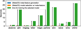
Figure 7: Time for MetaOD vs. training of the selected model (on 10 largest datasets in POC). MetaOD incurs only negligible overhead (diff. shown w/ black arrows).

References

- Abdulrahman et al. (2018) Abdulrahman, S. M., Brazdil, P., van Rijn, J. N., and Vanschoren, J. Speeding up algorithm selection using average ranking and active testing by introducing runtime. Mach. Learn., 107(1):79–108, 2018. URL http://dblp.uni-trier.de/db/journals/ml/ml107.html#AbdulrahmanBRV18.
- Aggarwal (2013) Aggarwal, C. C. Outlier Analysis. Springer, 2013. ISBN 978-1-4614-6396-2. URL http://dx.doi.org/10.1007/978-1-4614-6396-2.
- Bergstra & Bengio (2012) Bergstra, J. and Bengio, Y. Random search for hyper-parameter optimization. J. Mach. Learn. Res., 13:281–305, 2012. URL http://dblp.uni-trier.de/db/journals/jmlr/jmlr13.html#BergstraB12.
- Bharadhwaj (2019) Bharadhwaj, H. Meta-learning for user cold-start recommendation. In IJCNN, pp. 1–8. IEEE, 2019. ISBN 978-1-7281-1985-4. URL http://dblp.uni-trier.de/db/conf/ijcnn/ijcnn2019.html#Bharadhwaj19.
- Breunig et al. (2000) Breunig, M. M., Kriegel, H.-P., Ng, R. T., and Sander, J. Lof: Identifying density-based local outliers. In Chen, W., Naughton, J. F., and Bernstein, P. A. (eds.), SIGMOD Conference, pp. 93–104. ACM, 2000. ISBN 1-58113-217-4. URL http://dblp.uni-trier.de/db/conf/sigmod/sigmod2000.html#BreunigKNS00. SIGMOD Record 29(2), June 2000.
- Burnaev et al. (2015) Burnaev, E., Erofeev, P., and Smolyakov, D. Model selection for anomaly detection. In Verikas, A., Radeva, P., and Nikolaev, D. P. (eds.), ICMV, volume 9875 of SPIE Proceedings, pp. 987525. SPIE, 2015. ISBN 9781510601161. URL http://dblp.uni-trier.de/db/conf/icmv/icmv2015.html#BurnaevES15.
- Campos et al. (2016) Campos, G. O., Zimek, A., Sander, J., Campello, R. J. G. B., Micenková, B., Schubert, E., Assent, I., and Houle, M. E. On the evaluation of unsupervised outlier detection: measures, datasets, and an empirical study. Data Min. Knowl. Discov., 30(4):891–927, 2016. URL http://dblp.uni-trier.de/db/journals/datamine/datamine30.html#CamposZSCMSAH16.
- Chen et al. (2017) Chen, J., Sathe, S., Aggarwal, C. C., and Turaga, D. S. Outlier detection with autoencoder ensembles. In Chawla, N. V. and Wang, W. (eds.), Proceedings of the 2017 SIAM International Conference on Data Mining, Houston, Texas, USA, April 27-29, 2017, pp. 90–98. SIAM, 2017. doi: 10.1137/1.9781611974973.11. URL https://doi.org/10.1137/1.9781611974973.11.
- Deng & Xu (2007) Deng, H. and Xu, R. Model selection for anomaly detection in wireless ad hoc networks. In CIDM, pp. 540–546. IEEE, 2007. ISBN 1-4244-0705-2. URL http://dblp.uni-trier.de/db/conf/cidm/cidm2007.html#DengX07.
- Emmott et al. (2016) Emmott, A., Das, S., Dietterich, T. G., Fern, A., and Wong, W.-K. Anomaly detection meta-analysis benchmarks. 2016. URL https://ir.library.oregonstate.edu/concern/datasets/47429f155.
- Evangelista et al. (2007) Evangelista, P. F., Embrechts, M. J., and Szymanski, B. K. Some properties of the gaussian kernel for one class learning. In de Sá, J. M., Alexandre, L. A., Duch, W., and Mandic, D. P. (eds.), ICANN (1), volume 4668 of Lecture Notes in Computer Science, pp. 269–278. Springer, 2007. ISBN 978-3-540-74689-8. URL http://dblp.uni-trier.de/db/conf/icann/icann2007-1.html#EvangelistaES07.
- Fan et al. (2019) Fan, X., Yue, Y., Sarkar, P., and Wang, Y. X. R. A unified framework for tuning hyperparameters in clustering problems. CoRR, abs/1910.08018, 2019. URL http://dblp.uni-trier.de/db/journals/corr/corr1910.html#abs-1910-08018.
- Feurer & Hutter (2019) Feurer, M. and Hutter, F. Hyperparameter optimization. In Automated Machine Learning, pp. 3–33. Springer, Cham, 2019. URL https://link.springer.com/chapter/10.1007/978-3-030-05318-5_1.
- Feurer et al. (2015) Feurer, M., Springenberg, J. T., and Hutter, F. Initializing bayesian hyperparameter optimization via meta-learning. In Bonet, B. and Koenig, S. (eds.), Proceedings of the Twenty-Ninth AAAI Conference on Artificial Intelligence, January 25-30, 2015, Austin, Texas, USA, pp. 1128–1135. AAAI Press, 2015. URL http://www.aaai.org/ocs/index.php/AAAI/AAAI15/paper/view/10029.
- Feurer et al. (2018) Feurer, M., Letham, B., and Bakshy, E. Scalable meta-learning for bayesian optimization. CoRR, abs/1802.02219, 2018. URL http://dblp.uni-trier.de/db/journals/corr/corr1802.html#abs-1802-02219.
- Franceschi et al. (2017) Franceschi, L., Donini, M., Frasconi, P., and Pontil, M. Forward and reverse gradient-based hyperparameter optimization. In Precup, D. and Teh, Y. W. (eds.), Proceedings of the 34th International Conference on Machine Learning, ICML 2017, Sydney, NSW, Australia, 6-11 August 2017, volume 70 of Proceedings of Machine Learning Research, pp. 1165–1173. PMLR, 2017. URL http://proceedings.mlr.press/v70/franceschi17a.html.
- Fréry et al. (2017) Fréry, J., Habrard, A., Sebban, M., Caelen, O., and He-Guelton, L. Efficient top rank optimization with gradient boosting for supervised anomaly detection. In Ceci, M., Hollmén, J., Todorovski, L., Vens, C., and Dzeroski, S. (eds.), ECML/PKDD (1), volume 10534 of Lecture Notes in Computer Science, pp. 20–35. Springer, 2017. ISBN 978-3-319-71249-9. URL http://dblp.uni-trier.de/db/conf/pkdd/pkdd2017-1.html#FreryHSCH17.
- Goldstein & Dengel (2012) Goldstein, M. and Dengel, A. Histogram-based outlier score (hbos): A fast unsupervised anomaly detection algorithm. KI-2012: Poster and Demo Track, pp. 59–63, 2012. URL https://citeseerx.ist.psu.edu/viewdoc/download?doi=10.1.1.401.5686&rep=rep1&type=pdf.
- He et al. (2021) He, X., Zhao, K., and Chu, X. Automl: A survey of the state-of-the-art. Knowl. Based Syst., 212:106622, 2021. doi: 10.1016/j.knosys.2020.106622. URL https://doi.org/10.1016/j.knosys.2020.106622.
- Hutter et al. (2011) Hutter, F., Hoos, H. H., and Leyton-Brown, K. Sequential model-based optimization for general algorithm configuration. In Coello, C. A. C. (ed.), LION, volume 6683 of Lecture Notes in Computer Science, pp. 507–523. Springer, 2011. ISBN 978-3-642-25565-6. URL http://dblp.uni-trier.de/db/conf/lion/lion2011.html#HutterHL11.
- Idé & Kashima (2004) Idé, T. and Kashima, H. Eigenspace-based anomaly detection in computer systems. In Kim, W., Kohavi, R., Gehrke, J., and DuMouchel, W. (eds.), KDD, pp. 440–449. ACM, 2004. ISBN 1-58113-888-1. URL http://dblp.uni-trier.de/db/conf/kdd/kdd2004.html#IdeK04.
- Jones et al. (1998) Jones, D. R., Schonlau, M., and Welch, W. J. Efficient global optimization of expensive black-box functions. J. Global Optimization, 13(4):455–492, 1998. URL http://dblp.uni-trier.de/db/journals/jgo/jgo13.html#JonesSW98.
- Kadioglu et al. (2010) Kadioglu, S., Malitsky, Y., Sellmann, M., and Tierney, K. Isac - instance-specific algorithm configuration. In ECAI, volume 215 of Frontiers in Artificial Intelligence and Applications, pp. 751–756. IOS Press, 2010. URL http://dblp.uni-trier.de/db/conf/ecai/ecai2010.html#KadiogluMST10.
- Kriegel et al. (2008) Kriegel, H.-P., Schubert, M., and Zimek, A. Angle-based outlier detection in high-dimensional data. In Li, Y., Liu, B., and Sarawagi, S. (eds.), KDD, pp. 444–452. ACM, 2008. ISBN 978-1-60558-193-4. URL http://dblp.uni-trier.de/db/conf/kdd/kdd2008.html#KriegelSZ08.
- Lee et al. (2019) Lee, H., Im, J., Jang, S., Cho, H., and Chung, S. Melu: Meta-learned user preference estimator for cold-start recommendation. In Teredesai, A., Kumar, V., Li, Y., Rosales, R., Terzi, E., and Karypis, G. (eds.), KDD, pp. 1073–1082. ACM, 2019. ISBN 978-1-4503-6201-6. URL http://dblp.uni-trier.de/db/conf/kdd/kdd2019.html#LeeIJCC19.
- Li et al. (2017) Li, L., Jamieson, K. G., DeSalvo, G., Rostamizadeh, A., and Talwalkar, A. Hyperband: A novel bandit-based approach to hyperparameter optimization. J. Mach. Learn. Res., 18:185:1–185:52, 2017. URL http://dblp.uni-trier.de/db/journals/jmlr/jmlr18.html#LiJDRT17.
- Liu et al. (2008) Liu, F. T., Ting, K. M., and Zhou, Z.-H. Isolation forest. In ICDM, pp. 413–422. IEEE Computer Society, 2008. ISBN 978-0-7695-3502-9. URL http://dblp.uni-trier.de/db/conf/icdm/icdm2008.html#LiuTZ08.
- Misir & Sebag (2017) Misir, M. and Sebag, M. Alors: An algorithm recommender system. Artif. Intell., 244:291–314, 2017. URL http://dblp.uni-trier.de/db/journals/ai/ai244.html#MisirS17.
- Nikolic et al. (2013) Nikolic, M., Maric, F., and Janicic, P. Simple algorithm portfolio for sat. Artif. Intell. Rev., 40(4):457–465, 2013. URL http://dblp.uni-trier.de/db/journals/air/air40.html#NikolicMJ13.
- Pevný (2016) Pevný, T. Loda: Lightweight on-line detector of anomalies. Mach. Learn., 102(2):275–304, 2016. URL http://dblp.uni-trier.de/db/journals/ml/ml102.html#Pevny16.
- Ramaswamy et al. (2000) Ramaswamy, S., Rastogi, R., and Shim, K. Efficient algorithms for mining outliers from large data sets. In Chen, W., Naughton, J. F., and Bernstein, P. A. (eds.), SIGMOD Conference, pp. 427–438. ACM, 2000. ISBN 1-58113-217-4. URL http://dblp.uni-trier.de/db/conf/sigmod/sigmod2000.html#RamaswamyRS00. SIGMOD Record 29(2), June 2000.
- Rayana & Akoglu (2016) Rayana, S. and Akoglu, L. Less is more: Building selective anomaly ensembles. ACM Trans. Knowl. Discov. Data, 10(4):42:1–42:33, 2016. URL http://dblp.uni-trier.de/db/journals/tkdd/tkdd10.html#RayanaA16.
- Schölkopf et al. (1999) Schölkopf, B., Williamson, R. C., Smola, A. J., Shawe-Taylor, J., and Platt, J. C. Support vector method for novelty detection. In Solla, S. A., Leen, T. K., and Müller, K.-R. (eds.), NIPS, pp. 582–588. The MIT Press, 1999. ISBN 0-262-19450-3. URL http://dblp.uni-trier.de/db/conf/nips/nips1999.html#ScholkopfWSSP99.
- Schölkopf et al. (2001) Schölkopf, B., Platt, J. C., Shawe-Taylor, J., Smola, A. J., and Williamson, R. C. Estimating the support of a high-dimensional distribution. Neural Computation, 13(7):1443–1471, July 2001. doi: 10.1162/089976601750264965. URL https://doi.org/10.1162%2F089976601750264965.
- Shahriari et al. (2016) Shahriari, B., Swersky, K., Wang, Z., Adams, R. P., and de Freitas, N. Taking the human out of the loop: A review of bayesian optimization. Proc. IEEE, 104(1):148–175, 2016. doi: 10.1109/JPROC.2015.2494218. URL https://doi.org/10.1109/JPROC.2015.2494218.
- Shawi et al. (2019) Shawi, R. E., Maher, M., and Sakr, S. Automated machine learning: State-of-the-art and open challenges. CoRR, abs/1906.02287, 2019. URL http://arxiv.org/abs/1906.02287.
- Smith (2017) Smith, L. N. Cyclical learning rates for training neural networks. In WACV, pp. 464–472. IEEE Computer Society, 2017. ISBN 978-1-5090-4822-9. URL http://dblp.uni-trier.de/db/conf/wacv/wacv2017.html#Smith17.
- Stern et al. (2010) Stern, D. H., Samulowitz, H., Herbrich, R., Graepel, T., Pulina, L., and Tacchella, A. Collaborative expert portfolio management. In Fox, M. and Poole, D. (eds.), Proceedings of the Twenty-Fourth AAAI Conference on Artificial Intelligence, AAAI 2010, Atlanta, Georgia, USA, July 11-15, 2010. AAAI Press, 2010. URL http://www.aaai.org/ocs/index.php/AAAI/AAAI10/paper/view/1857.
- Tang et al. (2002) Tang, J., Chen, Z., Fu, A. W., and Cheung, D. W. Enhancing effectiveness of outlier detections for low density patterns. In Cheng, M., Yu, P. S., and Liu, B. (eds.), Advances in Knowledge Discovery and Data Mining, 6th Pacific-Asia Conference, PAKDD 2002, Taipei, Taiwan, May 6-8, 2002, Proceedings, volume 2336 of Lecture Notes in Computer Science, pp. 535–548. Springer, 2002. doi: 10.1007/3-540-47887-6“˙53. URL https://doi.org/10.1007/3-540-47887-6_53.
- Tax & Duin (2004) Tax, D. M. J. and Duin, R. P. W. Support vector data description. Mach. Learn., 54(1):45–66, 2004. doi: 10.1023/B:MACH.0000008084.60811.49. URL https://doi.org/10.1023/B:MACH.0000008084.60811.49.
- Vaithyanathan & Dom (1999) Vaithyanathan, S. and Dom, B. Generalized model selection for unsupervised learning in high dimensions. In Solla, S. A., Leen, T. K., and Müller, K.-R. (eds.), NIPS, pp. 970–976. The MIT Press, 1999. ISBN 0-262-19450-3. URL http://dblp.uni-trier.de/db/conf/nips/nips1999.html#VaithyanathanD99.
- Vanschoren (2018) Vanschoren, J. Meta-learning: A survey. CoRR, abs/1810.03548, 2018. URL http://dblp.uni-trier.de/db/journals/corr/corr1810.html#abs-1810-03548.
- Vartak et al. (2017) Vartak, M., Thiagarajan, A., Miranda, C., Bratman, J., and Larochelle, H. A meta-learning perspective on cold-start recommendations for items. In Guyon, I., von Luxburg, U., Bengio, S., Wallach, H. M., Fergus, R., Vishwanathan, S. V. N., and Garnett, R. (eds.), Advances in Neural Information Processing Systems 30: Annual Conference on Neural Information Processing Systems 2017, December 4-9, 2017, Long Beach, CA, USA, pp. 6904–6914, 2017. URL https://proceedings.neurips.cc/paper/2017/hash/51e6d6e679953c6311757004d8cbbba9-Abstract.html.
- Wistuba et al. (2015) Wistuba, M., Schilling, N., and Schmidt-Thieme, L. Learning hyperparameter optimization initializations. In DSAA, pp. 1–10. IEEE, 2015. URL http://dblp.uni-trier.de/db/conf/dsaa/dsaa2015.html#WistubaSS15.
- Wistuba et al. (2018) Wistuba, M., Schilling, N., and Schmidt-Thieme, L. Scalable gaussian process-based transfer surrogates for hyperparameter optimization. Mach. Learn., 107(1):43–78, 2018. URL http://dblp.uni-trier.de/db/journals/ml/ml107.html#WistubaSS18.
- Wolpert & Macready (1997) Wolpert, D. H. and Macready, W. G. No free lunch theorems for optimization. IEEE Trans. Evolutionary Computation, 1(1):67–82, 1997. URL http://dblp.uni-trier.de/db/journals/tec/tec1.html#DolpertM97.
- Xiao et al. (2014) Xiao, Y., Wang, H., Zhang, L., and Xu, W. Two methods of selecting gaussian kernel parameters for one-class svm and their application to fault detection. Knowl. Based Syst., 59:75–84, 2014. URL http://dblp.uni-trier.de/db/journals/kbs/kbs59.html#XiaoWZX14.
- Xu et al. (2012) Xu, L., Hutter, F., Shen, J., Hoos, H. H., and Leyton-Brown, K. Satzilla2012: Improved algorithm selection based on cost-sensitive classification models. Proceedings of SAT Challenge, pp. 57–58, 2012. URL http://citeseerx.ist.psu.edu/viewdoc/summary?doi=10.1.1.261.668.
- Yang & Shami (2020) Yang, L. and Shami, A. On hyperparameter optimization of machine learning algorithms: Theory and practice. Neurocomputing, 415:295–316, 2020. URL http://dblp.uni-trier.de/db/journals/ijon/ijon415.html#YangS20.
- Yao et al. (2018) Yao, Q., Wang, M., Escalante, H. J., Guyon, I., Hu, Y., Li, Y., Tu, W., Yang, Q., and Yu, Y. Taking human out of learning applications: A survey on automated machine learning. CoRR, abs/1810.13306, 2018. URL http://arxiv.org/abs/1810.13306.
- Yu & Zhu (2020) Yu, T. and Zhu, H. Hyper-parameter optimization: A review of algorithms and applications. CoRR, abs/2003.05689, 2020. URL https://arxiv.org/abs/2003.05689.
- Zhao et al. (2019) Zhao, Y., Nasrullah, Z., and Li, Z. Pyod: A python toolbox for scalable outlier detection. J. Mach. Learn. Res., 20:96:1–96:7, 2019. URL http://dblp.uni-trier.de/db/journals/jmlr/jmlr20.html#ZhaoNL19.
- Zhao et al. (2021) Zhao, Y., Hu, X., Cheng, C., Wang, C., Wan, C., Wang, W., Yang, J., Bai, H., Li, Z., Xiao, C., Wang, Y., Qiao, Z., Sun, J., and Akoglu, L. Suod: Accelerating large-scale unsupervised heterogeneous outlier detection. Proceedings of Machine Learning and Systems, 2021. URL https://arxiv.org/abs/2002.03222.
- Zheng et al. (2007) Zheng, Z., Yang, J., and Zhu, Y. Initialization enhancer for non-negative matrix factorization. Eng. Appl. Artif. Intell., 20(1):101–110, 2007. URL http://dblp.uni-trier.de/db/journals/eaai/eaai20.html#ZhengYZ07.
- Zhou & Paffenroth (2017) Zhou, C. and Paffenroth, R. C. Anomaly detection with robust deep autoencoders. In Proceedings of the 23rd ACM SIGKDD International Conference on Knowledge Discovery and Data Mining, Halifax, NS, Canada, August 13 - 17, 2017, pp. 665–674. ACM, 2017. doi: 10.1145/3097983.3098052. URL https://doi.org/10.1145/3097983.3098052.