Multiple timescales and the parametrisation method
in geometric singular perturbation theory

Abstract

We present a novel method for computing slow manifolds and their fast fibre bundles in geometric singular perturbation problems. This coordinate-independent method is inspired by the parametrisation method introduced by Cabré, Fontich and de la Llave. By iteratively solving a so-called conjugacy equation, our method simultaneously computes parametrisations of slow manifolds and fast fibre bundles, as well as the dynamics on these objects, to arbitrarily high degrees of accuracy. We show the power of this top-down method for the study of systems with multiple (i.e., three or more) timescales. In particular, we highlight the emergence of hidden timescales and show how our method can uncover these surprising multiple timescale structures. We also apply our parametrisation method to several reaction network problems.

1 Introduction

Many evolving biological and physical systems display distinct temporal features, which can be attributed to processes taking place on different timescales. In mathematical terms, such multiple timescale models are in fact singular perturbation problems. In this paper we consider parameter-dependent differential equations of the general form

$$x^{\prime}=\frac{dx}{dt}=F(x,\varepsilon)=\sum_{i=0}^{l}\varepsilon^{i}F_{i}(x)\,\qquad(l\geq 1)\,,$$ (1.1)

for $x\in\mathbb{R}^{n}$. Here, $0\leq\varepsilon\ll 1$ is a small perturbation parameter, and the smooth functions $F_{i}:\mathbb{R}^{n}\to\mathbb{R}^{n}$ model processes evolving on distinct timescales $t_{i}=\varepsilon^{i}t$.

In the case that the zero-limit critical set

$$S:=\{x\in\mathbb{R}^{n}\,:\,F_{0}(x)=0\}$$

contains a $k$-dimensional differentiable critical manifold $S_{0}\subseteq S$, with $1\leq k\leq n-1$, system (1.1) is considered a singular perturbation problem. The slower processes $F_{i}\,(i\geq 1)$ will then determine the dynamics of the model in phase space near $S_{0}$.

A classical theorem of Fenichel [11] guarantees that the (compact) critical manifold $S_{0}$ persists as a flow-invariant slow manifold $S_{0}^{\varepsilon}$ in any dynamical system close to the singular limit $x^{\prime}=F_{0}(x)$, under the condition that the critical manifold $S_{0}$ is normally hyperbolic. The corresponding slow flow on $S_{0}^{\varepsilon}$ is then governed to leading order by the reduced problem

$$\dot{x}=P_{0}(x)F_{1}(x)\,,\qquad\forall x\in S_{0}\,,$$ (1.2)

where the overdot indicates differentation with respect to the slow time $t_{1}=\varepsilon t$, and $P_{0}$ is a certain (unique) projection onto the tangent bundle ${\cal T}S_{0}$. This geometric singular perturbation theory (GSPT) result due to Fenichel not only describes the persistence of an invariant slow manifold $S_{0}^{\varepsilon}$ near $S_{0}$, but also the (local) persistence of an invariant nonlinear fast fibre bundle ${\cal L}S_{0}^{\varepsilon}$ that describes the fast dynamics towards or away from the slow manifold $S_{0}^{\varepsilon}$.

Under the basic assumption that the critical manifold $S_{0}$ is the image of a smooth embedding $\phi_{0}:U_{1}\to\mathbb{R}^{n}$ defined on an open subset $U_{1}\subset\mathbb{R}^{k}$, the $k$-dimensional reduced leading order problem (1.2) can alternatively be described in the (local) coordinate chart $U_{1}$ by the differential equation

$$\dot{\xi}=r_{1}(\xi):=L_{0}(\xi)\,P_{0}F_{1}(\phi_{0}(\xi))\ \ \mbox{for}\ \xi\in U_{1}\,.$$ (1.3)

Here, $L_{0}(\xi)D\phi_{0}(\xi)={\rm id}_{\mathbb{R}^{k}},\,\forall\xi\in U_{1}$, i.e., $L_{0}(\xi)$ is a left inverse of $D\phi_{0}(\xi)$; see, e.g., Feliu et al [10]. In this paper, we build upon this local representation in a coordinate chart, and we provide an alternative way to compute it, by introducing a parametrisation method for finding slow invariant manifolds and their linear fast fibre bundles, to any order in the small parameter, and for general coordinate-independent multiple timescale problems of the form (1.1). A key observation underlying our method is that the identification of these manifolds and bundles can be reframed in terms of solving a so-called conjugacy equation. A solution to this conjugacy equation consists of embeddings of the slow manifold and corresponding linear fast fibre bundle, as well as the slow and fast vector fields that they carry (in the appropriate coordinate chart). Our parametrisation method seeks to iteratively solve the conjugacy equation, thereby calculating the slow and fast dynamics to arbitrary precision.

To the best of our knowledge this paper presents the first parametrisation method for singular perturbation problems. At the same time, the idea to compute invariant manifolds by solving a conjugacy equation is of course classical. A well-known example is the Lyapunov-Schmidt method for computing periodic orbits near Hopf bifurcations. In this setting, the problem is phrased as a conjugacy equation on a loop space, which can be solved with the implicit function theorem, see for instance [9, 14, 35]. The idea is also very prominent in the work of Cabré, Fontich and de la Llave, who introduced a parametrisation method in the early 2000’s. More precisely, in [3, 4, 5] they provide an iterative scheme for computing stable and unstable manifolds of hyperbolic fixed points of maps and flows, and analytically prove the convergence of this scheme. The scope of their method has since been extended considerably, for example to delay equations [17] and partial differential equations [30], and variants of the method have been introduced to compute, e.g. KAM tori [15] and centre manifolds [2]. We refer to [18] for an extensive list of references and an overview of results.

We should mention in particular the work of Haro and Canadell [6], who introduced a parametrisation method for computing normally hyperbolic invariant manifolds. Their method consists of a Newton iteration, and it was used to numerically compute normally hyperbolic quasi-periodic tori in Hamiltonian systems. For such quasi-periodic tori, their method was proved to converge in [7]. The setting of the current paper is similar in nature: we present a parametrisation method for slow manifolds, which are also normally hyperbolic invariant manifolds, but having the additional property that the flow that they carry is close to stationary. This latter property allows us to provide explicit analytical formulas for the solutions to the homological equations that arise in each step of the iteration, see for example the proofs of Theorem 2.13 and Theorem 2.18. Such analytical formulas are not available for the iterative method in [6, 7]. On the other hand, in contrast with [6, 7], the iterative scheme that we provide here is a quasi-Newton method, and hence not quadratically but linearly convergent.

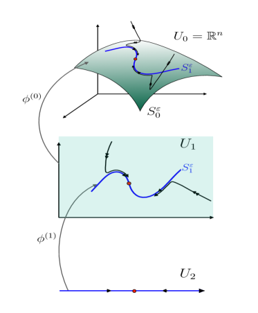
Figure 1: Sketch of a multiple timescale dynamical system having two nested slow invariant manifolds $S_{0}^{\varepsilon}$ and $S_{1}^{\varepsilon}$. The coordinate chart $U_{1}$ is embedded as $S_{0}^{\varepsilon}\subset U_{0}=\mathbb{R}^{n}$ by $\phi^{(0)}$, and the coordinate chart $U_{2}$ is embedded as $S_{1}^{\varepsilon}\subset U_{1}$ by $\phi^{(1)}$ (this superscript notation ⁽ⁱ⁾ will be introduced in section 3). The red point depicts the possibility of a lower-dimensional invariant object (e.g. an equilibrium point, or a further submanifold introducing yet another dynamical timescale). The parametrisation method introduced in this article uses a top-down approach, i.e. the slow manifold $S_{0}^{\varepsilon}$ is identified first, then the infra-slow manifold $S_{1}^{\varepsilon}$, etc.

The parametrisation method becomes particularly useful when dealing with genuine singularly perturbed multiple timescale problems in which the slow flow on the slow manifold $S_{0}^{\varepsilon}$ is a singular perturbation problem itself, i.e., if there exists an embedded lower-dimensional infra-slow invariant manifold $S_{1}^{\varepsilon}\subset S_{0}^{\varepsilon}$ where processes on the timescale $t_{2}=\varepsilon^{2}t$ become dominant. Note that the equation $\dot{\xi}=r_{1}(\xi)+\mathcal{O}(\varepsilon)$ on the coordinate chart $U_{1}$ is itself a singular perturbation problem when $S_{1}=\{\xi\in U_{1}\,:\,r_{1}(\xi)=0\}$ contains a critical manifold of dimension $1\leq n_{2}\leq k-1$. This simple observation will lead to a geometric definition of a singularly perturbed multiple timescale system, possessing nested invariant (slow, infra-slow,…) manifolds $S_{0}^{\varepsilon}\supset S_{1}^{\varepsilon}\supset\cdots\supset S_{m-2}^{\varepsilon}$ that support flows evolving on distinct (slow, infra-slow,…) timescales $t_{1}=\varepsilon t,\,t_{2}=\varepsilon^{2}t\,,\ldots,t_{m-1}=\varepsilon^{m-1}t$. We provide algorithms to calculate these nested slow manifolds, and their slow flows, using a top-down approach: our method calculates the ‘top’ slow manifold $S_{0}^{\varepsilon}$ first, and then makes its way ‘down’ the chain of nested slow manifolds; see Figure 1.

First theoretical results on multiple timescale problems have been provided by Cardin & Teixeira [8] who studied multiple timescale problems given in the standard form

$$x_{j}^{\prime} =\left(\prod_{i=0}^{m-j}\varepsilon_{i}\right)f_{j}(x,\varepsilon)\,,\quad j=1,\ldots,m\,,$$ (1.4)

where $x=(x_{1},\ldots,x_{m})\in\mathbb{R}^{n}$, $m\geq 2$, $x_{j}\in\mathbb{R}^{l_{j}}$, $\sum_{j=1}^{m}l_{j}=n$, $\varepsilon_{0}=1$ and $\varepsilon=(\varepsilon_{1},\ldots,\varepsilon_{m})$ is a vector of independent small parameters $\varepsilon_{1},\ldots,\varepsilon_{m}\ll 1$. In this standard framework, the underlying multiple timescale processes are identified with specific coordinates: $x_{m}$ is a fast variable, $x_{m-1}$ is a slow variable, …, $x_{1}$ is the slowest variable. Here, one may also identify the nested invariant (critical) manifolds $S_{0}\supset S_{1}\supset\cdots\supset S_{m-2}$ a-priori as the zero sets

$$S_{l}=\{x\in\mathbb{R}^{n}:f_{j}(x,0)=0,\;j=1,\ldots l+1\}\,,\quad l=0,\ldots m-2\,.$$ (1.5)

Assuming that these nested critical manifolds $S_{l}$ are all normally hyperbolic, the authors of [8] show the persistence of nested invariant (slow, infra-slow,…) manifolds $S_{0}^{\varepsilon}\supset S_{1}^{\varepsilon}\supset\cdots\supset S_{m-2}^{\varepsilon}$. In contrast to our proposed top-down approach, their proof follows a bottom-up approach, i.e., they first show the existence of the ‘bottom’ manifold $S_{m-2}^{\varepsilon}$ based on Fenichel theory, and then work their way ‘up’ to the top manifold $S_{0}^{\varepsilon}$. We also note that the independence of the small parameters $\varepsilon=(\varepsilon_{1},\ldots,\varepsilon_{m})$ is crucial in their proof. Recently, Kruff & Walcher [22] provided first results on three timescale problems in a nonstandard, coordinate independent setting. Their approach is based on transforming a coordinate-independent system into a (local) standard form first, and then applying the results of Cardin & Teixeira.

We would like to point out that the nested sets given by (1.5) are restrictive when it comes to identifying multiple timescale structures in singular perturbation problems, i.e. the bottom-up approach relies on a priori knowledge of ultimate attractor states and/or the number of timescales involved in the dynamics. In the following example, we highlight some of the subtleties that may arise in general multiple timescale dynamics.

Example 1.1.

Let us consider the following (reaction) network motif

describing an incoherent feed-forward loop (IFFL) with three reactants; see e.g. [1]. In dimensionless form, the evolution equations for the reactant concentrations that govern a very simple form of such an IFFL, are

$$\frac{d}{dt}\left(\begin{array}[]{c}x_{1}\\ x_{2}\\ x_{3}\end{array}\right)=\underbrace{\left(\begin{array}[]{c}0\\ 0\\ -x_{3}\end{array}\right)}_{F_{0}(x)}+\varepsilon\underbrace{\left(\begin{array}[]{c}a_{1}x_{3}-a_{2}x_{1}x_{2}\\ a_{3}x_{3}-a_{4}x_{2}\\ 1\end{array}\right)}_{F_{1}(x)}\,\,.$$ (1.15)

Here, $0<\varepsilon\ll 1$ is a small parameter, i.e., we assume that the decay rate of $x_{3}$ is significantly faster than all other reaction rates, but we assume that all other parameters $a_{i}=O(1)$, $i=1,\ldots,4$, are of the same order.

Firstly, we notice that this reaction network is governed by two processes, one fast process $F_{0}$ and one slow process $F_{1}$. System (1.15) is actually of the standard form (1.4), i.e., $x_{3}$ is considered a fast variable while $(x_{1},x_{2})$ are slow variables. One may therefore naively expect to deal with a standard two timescale problem. It turns out that this intuition is incorrect.

To see this, note that the critical manifold $S_{0}=\{(x_{1},x_{2},x_{3})\in\mathbb{R}^{3}:x_{3}=0\}$ is a two-dimensional plane. In fact, because $\frac{dx_{3}}{dt}=-x_{3}+\varepsilon$, every solution converges exponentially to the nearby invariant slow manifold $S_{0}^{\varepsilon}=\{(x_{1},x_{2},x_{3})\in\mathbb{R}^{3}:x_{3}=\varepsilon\}$. The slow dynamics on $S_{0}^{\varepsilon}$ is governed by the two-dimensional system

$$\frac{d}{dt_{1}}\left(\begin{array}[]{c}\ x_{1}\\ x_{2}\end{array}\right)=\underbrace{\left(\begin{array}[]{c}-a_{2}x_{1}x_{2}\\ -a_{4}x_{2}\end{array}\right)}_{r_{1}(x_{1},x_{2})}+\varepsilon\underbrace{\left(\begin{array}[]{c}a_{1}\\ a_{3}\end{array}\right)}_{r_{2}(x_{1},x_{2})}\,,$$ (1.22)

where $t_{1}=\varepsilon t$ is a slow time variable. Observe now that system (1.22) is another two timescale problem, but this time in the nonstandard form (1.1). The one-dimensional critical manifold of system (1.22) is $S_{1}=\{(x_{1},x_{2})\in\mathbb{R}^{2}:x_{2}=0\}$, a line. Because

$$\frac{dx_{2}}{dt_{1}}=-a_{4}x_{2}+\varepsilon a_{3}\,,$$

we also see that every solution to (1.22) converges exponentially (in the slow time $t_{1}$) to the infra-slow one-dimensional invariant manifold $S_{1}^{\varepsilon}=\{(x_{1},x_{2})\in\mathbb{R}^{2}:x_{2}=\varepsilon\frac{a_{3}}{a_{4}}\}$. The infra-slow dynamics on $S_{1}^{\varepsilon}$ is in turn governed by

$$\frac{dx_{1}}{dt_{2}} =a_{1}-\frac{a_{2}a_{3}}{a_{4}}x_{1}\,,$$ (1.23)

where $t_{2}=\varepsilon^{2}t$ is an infra-slow time variable. The infra-slow flow on $S_{1}^{\varepsilon}$ in fact converges to the equilibrium $x_{1}=\frac{a_{1}a_{4}}{a_{2}a_{3}}$ corresponding to the unique equilibrium state $(x_{1},x_{2},x_{3})=(\frac{a_{1}a_{4}}{a_{2}a_{3}},\varepsilon\frac{a_{3}}{a_{4}},\varepsilon)$ of system (1.15). Remarkably, and perhaps counter-intuitively, we thus find that system (1.15) actually evolves on three different timescales.

We would like to point out that our direct computations followed a top-down approach, i.e. we algorithmically discovered the hidden multiple timescale structure through computing the slow vector field (1.22) in a coordinate chart for the slow manifold $S_{0}^{\varepsilon}$, and then identifying (1.22) as another singular perturbation problem. We note that one can also identify the three disparate timescales (locally) in this simple example by computing the Jacobian at the unique attracting equilibrium, which is given in upper triangular form

$$\begin{pmatrix}-\varepsilon^{2}\frac{a_{2}a_{3}}{a_{4}}&-\varepsilon\frac{a_{1}a_{4}}{a_{3}}&\varepsilon a_{1}\\ 0&-\varepsilon a_{4}&\varepsilon a_{3}\\ 0&0&-1\end{pmatrix}\,.$$

We emphasize that a priori knowledge (or even existence) of a unique attractor state in general multiple timescale systems is usually exceptional. Hence, any method to identify multiple timescales dynamics should not necessarily rely on this.

$\triangle$

In general, the slow and infra-slow manifolds of a singular perturbation problem cannot be computed as easily as in the above simple example. As a result, it will be hard to predict which, and how many, timescales a singular perturbation problem will possess. The parametrisation method presented in this paper will take care of this problem and provide the algorithms needed to define and compute slow and infra-slow manifolds and their flows, in arbitrary multiple timescale problems of the form (1.1).

There are already several (families of) algorithms which compute approximations to invariant objects in two-timescale dynamical systems. These include the computational singular perturbation (CSP) method [23, 24], the zero-derivative principle [12], and the method of intrinsic low-dimensional manifolds [27, 28]. Our parametrisation method shares some similarities with the CSP method, which also iteratively computes slow manifolds and fast fibres. A distinction is often drawn between the one-step and two-step versions of CSP which approximate, respectively, the slow manifold alone versus the slow manifold and the linear fast fibre bundle simultaneously. Analogously, our parametrisation method is also capable of approximating the slow manifold independently. The CSP method has been implemented for the class of coordinate independent problems of the form (1.1) in [26], building on rigorous convergence and coordinate-independence results in [21, 29, 34, 37, 38]. We emphasize that our parametrisation method wields the further advantage of being naturally applicable in multiple timescale problems.

The remainder of this paper is organised as follows. In section 2, we introduce the parametrisation method in the setting of two-timescale problems. We show how the method can be used to compute slow manifolds and their linear fast fibre bundles, and we prove that the method formally converges. In section 3, we give a definition of a geometric singular perturbation problem with multiple timescales, and we discuss in some detail the mechanism by which ‘hidden’ timescales can emerge. In section 4, we apply the parametrisation method to two different reaction networks. We conclude with some remarks in section 5.

2 The parametrisation method in two-timescale problems

In this section, we introduce the parametrisation method for finding slow manifolds and their fast fibre bundles in geometric singular perturbation problems of the general form (1.1).

2.1 Setup

Let $\varepsilon_{0}>0$, let $U_{0}\subseteq\mathbb{R}^{n}$ be an open subset, and consider a smooth parameter-dependent vector field $F:U_{0}\times[0,\varepsilon_{0})\to\mathbb{R}^{n}$ of the form

$$F(x,\varepsilon)=\sum_{i=0}^{l}\varepsilon^{i}F_{i}(x)\,\qquad(l\geq 1)\,.$$

Our crucial assumption will be that $F_{0}:U_{0}\subseteq\mathbb{R}^{n}\to\mathbb{R}^{n}$ admits a smooth $k$-dimensional manifold $S_{0}$ of critical points, where we only consider the case that $S_{0}$ is nontrivial, i.e., that $1\leq k\leq n-1$. More specifically, we will assume that $S_{0}$ is the image of a smooth embedding

$$\phi_{0}:U_{1}\to U_{0}\subseteq\mathbb{R}^{n}\,,$$

where $U_{1}\subset\mathbb{R}^{k}$ is an open set.

Our first goal is to find an invariant manifold $S_{0}^{\varepsilon}$ close to $S_{0}$ for the perturbation $F$ of $F_{0}$. We do this by searching for an embedding $\phi$ of $S_{0}^{\varepsilon}$ with an asymptotic expansion of the form

$$\phi=\phi(\xi,\varepsilon)=\phi_{0}(\xi)+\varepsilon\phi_{1}(\xi)+\varepsilon^{2}\phi_{2}(\xi)+\ldots:U_{1}\times[0,\varepsilon_{0})\to\mathbb{R}^{n}\,.$$

It holds that $\phi(U_{1},\varepsilon)$ is invariant under the flow of $F(\cdot,\varepsilon)$, for all $\varepsilon\in[0,\varepsilon_{0})$, if there is a vector field

$$r=r(\xi,\varepsilon)=\varepsilon r_{1}(\xi)+\varepsilon^{2}r_{2}(\xi)+\ldots:U_{1}\times[0,\varepsilon_{0})\to\mathbb{R}^{k}$$

with the property that whenever $\xi(t)$ satisfies $\frac{d\xi}{dt}=r(\xi,\varepsilon)$, then $x(t):=\phi(\xi(t),\varepsilon)$ satisfies $\frac{dx}{dt}=F(x,\varepsilon)$. In other words, if the pair $(\phi,r):U_{1}\times[0,\varepsilon_{0})\to\mathbb{R}^{n}\times\mathbb{R}^{k}$ satisfies the conjugacy equation

$$\mathcal{F}(\phi,r)(\xi,\varepsilon):=D\phi(\xi,\varepsilon)\cdot r(\xi,\varepsilon)-F(\phi(\xi,\varepsilon),\varepsilon)=0\,.$$ (2.1)

Here $D=D_{x}$ denotes differentiation to the first variable only. In particular, it follows from (2.1) that $F(\phi(\xi,\varepsilon),\varepsilon)=D\phi(\xi,\varepsilon)\cdot r(\xi,\varepsilon)\in T_{\phi(\xi,\varepsilon)}\left(\phi(U_{1},\varepsilon)\right)$. This means that $F(\phi(\xi),\varepsilon)$ is tangent to $S_{0}^{\varepsilon}:=\phi(U_{1},\varepsilon)$, and hence that $S_{0}^{\varepsilon}$ is invariant under the flow of $F(\cdot,\varepsilon)$.

Remark 2.1.

One can equivalently represent equation (2.1) by the commuting diagram

where $T\phi(\xi,v,\varepsilon):=(\phi(\xi,\varepsilon),D\phi(\xi,\varepsilon)\cdot v)$. Note that we have suppressed the dependence on the parameter $\varepsilon\in[0,\varepsilon_{0})$ in the diagram for clarity. $\triangle$

We will now attempt to solve the conjugacy equation (2.1) by an iterative procedure. In fact, expansion of (2.1) in powers of $\varepsilon$ yields a recurrence relation for the unknowns $(\phi_{i},r_{i})$. The first of these is the equation $F_{0}\circ\phi_{0}=0$, which holds by definition of $S_{0}$. The remaining relations are the following (here we don’t write the dependence on $\xi$):

$$\begin{array}[]{lll}D\phi_{0}\cdot r_{1}-DF_{0}(\phi_{0})\cdot\phi_{1}=&F_{1}(\phi_{0})&=:G_{1}\\ D\phi_{0}\cdot r_{2}-DF_{0}(\phi_{0})\cdot\phi_{2}=&-D\phi_{1}\cdot r_{1}+F_{2}(\phi_{0})&\\ &+DF_{1}(\phi_{0})\cdot\phi_{1}+\frac{1}{2}D^{2}F_{0}(\phi_{0})(\phi_{1},\phi_{1})&=:G_{2}\\ \vdots&\vdots&\vdots\\ D\phi_{0}\cdot r_{i}-DF_{0}(\phi_{0})\cdot\phi_{i}=&G_{i}(\phi_{0},\ldots,\phi_{i-1},r_{1},\ldots,r_{i-1})&=:G_{i}\\ \vdots&\vdots&\vdots\end{array}$$ (2.8)

The $i$-th equation in this list is an inhomogeneous linear equation for $r_{i}$ and $\phi_{i}$, of the form

$$D\mathcal{F}(\phi_{0},0)\cdot(\phi_{i},r_{i})=D\phi_{0}\cdot r_{i}-DF_{0}(\phi_{0})\cdot\phi_{i}=G_{i}\,.$$ (2.9)

We shall refer to this equation as the infinitesimal conjugacy equation. The inhomogeneous term $G_{i}=G_{i}(\xi)$ in this equation only depends on the $\phi_{j}$ and $r_{j}$ with $0\leq j<i$. The recursively defined infinitesimal conjugacy equations can therefore be solved iteratively for $(\phi_{i},r_{i})$ under the condition that the linear operator $D\mathcal{F}(\phi_{0},0)$ is surjective.

Remark 2.2.

In many applications, multiple timescale models are given by a polynomial vector field $F(x,\varepsilon)$ with the property that the leading order term can be factored as

$$F(x,0)=F_{0}(x) ={\bf N}_{0}(x)\cdot f_{0}(x)\,,$$ (2.10)

with matrix ${\bf N}_{0}:U_{0}\to L(\mathbb{R}^{n-k},\mathbb{R}^{n})$ and vector $f_{0}:U_{0}\to\mathbb{R}^{n-k}$. If we assume that this matrix ${\bf N}_{0}(x)$ has full rank $n-k$ for all $x\in S_{0}$, then $F_{0}(x)=0$ if and only if $f_{0}(x)=0$. The critical manifold is then given by $S_{0}=\{x\in U_{0}\,|\,f_{0}(x)=0\}$. This $S_{0}$ is indeed a manifold of dimension $k$, if it holds that $Df_{0}(x):\mathbb{R}^{n}\to\mathbb{R}^{n-k}$ is surjective for all $x\in S_{0}$. The operator $D\mathcal{F}(\phi_{0},0)$ is given in this case by

$$D\mathcal{F}(\phi_{0},0)\cdot(\phi_{i},r_{i}) =\begin{pmatrix}-{\bf N}_{0}(\phi_{0})\cdot Df_{0}(\phi_{0})&D\phi_{0}\end{pmatrix}\begin{pmatrix}\phi_{i}\\ r_{i}\end{pmatrix}.$$ (2.11)

$\triangle$

Example 2.3.

Consider the planar system

$$\left.\begin{array}[]{ll}\begin{pmatrix}x_{1}^{\prime}\\ x_{2}^{\prime}\end{pmatrix}&=\begin{pmatrix}2x_{1}\\ x_{2}\end{pmatrix}(1-x_{2}-x_{1}^{2})+\varepsilon\begin{pmatrix}2\\ -x_{1}\end{pmatrix}\vspace{0.3 cm}\\ &=F_{0}(x_{1},x_{2})+\varepsilon F_{1}(x_{1},x_{2})\end{array}\right.$$ (2.14)

with $0\leq\varepsilon\ll 1$. Observe that (2.14) is written with the leading-order part $F_{0}$ in the factored form (2.10). The critical manifold

$$S_{0}=\{(x_{1},x_{2}):F_{0}(x_{1},x_{2})=0\}=\{(x_{1},x_{2}):\,x_{2}=1-x_{1}^{2}\}\,$$

is a parabola, embedded for example by the smooth map

$$\phi_{0}(\xi) =\begin{pmatrix}\xi\\ f_{0}(\xi)\end{pmatrix}=\begin{pmatrix}\xi\\ 1-\xi^{2}\end{pmatrix}.$$ (2.15)

Recalling that the operator $D\mathcal{F}(\phi_{0},0)$ can also be written in the form (2.11), one may compute that it is given by

$$D\mathcal{F}(\phi_{0},0)\,\begin{pmatrix}\phi_{i,1}\\ \phi_{i,2}\\ r_{i}\end{pmatrix}(\xi)=\begin{pmatrix}4\xi^{2}&2\xi&1\\ 2\xi(1-\xi^{2})&1-\xi^{2}&-2\xi\end{pmatrix}\begin{pmatrix}\phi_{i,1}(\xi)\\ \phi_{i,2}(\xi)\\ r_{i}(\xi)\end{pmatrix}\,.$$

We now make a ‘graph style’ ansatz for the embedding $\phi$ of $S^{\varepsilon}_{0}$; that is, we take $\phi(\xi,\varepsilon)=(\xi,f_{0}(\xi)+\varepsilon f_{1}(\xi)+\varepsilon^{2}f_{2}(\xi)+\cdots)$. Equivalently, we choose

$$\phi_{i}(\xi) =\begin{pmatrix}\phi_{i,1}(\xi)\\ \phi_{i,2}(\xi)\end{pmatrix}=\begin{pmatrix}0\\ f_{i}(\xi)\end{pmatrix}.$$

It turns out that with this choice, the surjective operator $D\mathcal{F}(\phi_{0},0)$ becomes an invertible operator $\Pi$ acting on $(f_{i},r_{i})$, because

$$\begin{pmatrix}4\xi^{2}&2\xi&1\\ 2\xi(1-\xi^{2})&1-\xi^{2}&-2\xi\end{pmatrix}\begin{pmatrix}0\\ f_{i}(\xi)\\ r_{i}(\xi)\end{pmatrix}=\begin{pmatrix}2\xi&1\\ 1-\xi^{2}&-2\xi\end{pmatrix}\begin{pmatrix}f_{i}(\xi)\\ r_{i}(\xi)\end{pmatrix}=:\Pi(\xi)\begin{pmatrix}f_{i}(\xi)\\ r_{i}(\xi)\end{pmatrix}\,,$$

and $\Delta=\Delta(\xi):=-\det\Pi(\xi)=1+3\xi^{2}>0$. We thus obtain the iterative formula

$$\begin{pmatrix}f_{i}(\xi)\\ r_{i}(\xi)\end{pmatrix} =\Pi(\xi)^{-1}G_{i}(\xi)=\frac{1}{\Delta}\begin{pmatrix}2\xi&1\\ 1-\xi^{2}&-2\xi\end{pmatrix}G_{i}(\xi)\,.$$ (2.16)

We proceed to compute the terms $r_{1},f_{1},r_{2},f_{2}$ explicitly. Using (2.16) with $i=1$, we have

$$\begin{pmatrix}f_{1}(\xi)\\ r_{1}(\xi)\end{pmatrix} =\frac{1}{\Delta}\begin{pmatrix}2\xi&1\\ 1-\xi^{2}&-2\xi\end{pmatrix}F_{1}(\phi_{0}(\xi))$$

$$=\frac{1}{\Delta}\begin{pmatrix}2\xi&1\\ 1-\xi^{2}&-2\xi\end{pmatrix}\begin{pmatrix}2\\ -\xi\end{pmatrix}=\frac{1}{\Delta}\begin{pmatrix}3\xi\\ 2\end{pmatrix}.$$

We then compute $G_{2}$:

$$G_{2}(\xi) =-D\phi_{1}(\xi)\cdot r_{1}(\xi)+F_{2}(\phi_{0}(\xi))+DF_{1}(\phi_{0}(\xi))\cdot\phi_{1}(\xi)+\frac{1}{2}D^{2}F_{0}(\phi_{0}(\xi))(\phi_{1}(\xi),\phi_{1}(\xi))$$

$$=\begin{pmatrix}0\\ (18\xi^{2}-6)/\Delta^{3}\end{pmatrix}+\begin{pmatrix}0\\ 0\end{pmatrix}+\begin{pmatrix}0\\ 0\end{pmatrix}+\begin{pmatrix}0\\ -9\xi^{2}/\Delta^{2}\end{pmatrix}=\begin{pmatrix}0\\ -3(9\xi^{4}-3\xi^{2}+2)/\Delta^{3}\end{pmatrix}.$$

So using (2.16) for $i=2$, we find

$$\begin{pmatrix}f_{2}(\xi)\\ r_{2}(\xi)\end{pmatrix} =\frac{1}{\Delta}\begin{pmatrix}2\xi&1\\ 1-\xi^{2}&-2\xi\end{pmatrix}\begin{pmatrix}0\\ -3(9\xi^{4}-3\xi^{2}+2)/\Delta^{3}\end{pmatrix}=\frac{1}{\Delta^{4}}\begin{pmatrix}-3(9\xi^{4}-3\xi^{2}+2)\\ 6\xi(9\xi^{4}-3\xi^{2}+2)\end{pmatrix}.$$

Altogether, this produces the asymptotic expansions

$$r(\xi,\varepsilon) =\varepsilon\left(\frac{2}{\Delta}\right)+\varepsilon^{2}\frac{6\xi(9\xi^{4}-3\xi^{2}+2)}{\Delta^{4}}+\mathcal{O}(\varepsilon^{3})\,,$$

$$\phi(\xi,\varepsilon) =\left(\xi,1-\xi^{2}+\varepsilon\left(\frac{3\xi}{\Delta}\right)+\varepsilon^{2}\left(\frac{-3(9\xi^{4}-3\xi^{2}+2)}{\Delta^{4}}\right)+\mathcal{O}(\varepsilon^{3})\right)\,.$$

We finish this example by pointing out that the embedding $\phi$ of a slow manifold $S_{0}^{\varepsilon}$ is not unique; correspondingly, there are many ways to obtain invertible restrictions of the surjective operator $D\mathcal{F}(\phi_{0},0)$. For example, if we let

$$\phi_{i}(\xi) =\begin{pmatrix}A(\xi)\\ B(\xi)\end{pmatrix}g_{i}(\xi)\,,$$

with $A,B,g_{i}$ smooth scalar functions, then

$$D\mathcal{F}(\phi_{0},0)\,\begin{pmatrix}\phi_{i,1}\\ \phi_{i,2}\\ r_{i}\end{pmatrix}(\xi) =\begin{pmatrix}(B(\xi)+2A(\xi)\xi)(2\xi)&1\\ (B(\xi)+2A(\xi)\xi)(1-\xi^{2})&-2\xi\end{pmatrix}\begin{pmatrix}g_{i}(\xi)\\ r_{i}(\xi)\end{pmatrix},$$

and so the operator $D\mathcal{F}(\phi_{0},0)$ restricts to an invertible operator for any nontrivial choice of $A(\xi)$ and $B(\xi)$, except if $B(\xi)=-2\xi A(\xi)$ for some $\xi$. The latter is the case precisely when

$$\begin{pmatrix}A(\xi)\\ B(\xi)\end{pmatrix} =\begin{pmatrix}1\\ -2\xi\end{pmatrix}A(\xi)\in\text{im\leavevmode\nobreak\ }D\phi_{0}(\xi).$$ (2.17)

The iteration is thus well-defined as long as we seek $\phi_{i}$ that do not lie in the direction tangent to $S_{0}$. The choice of $A,B$ in the present example will nevertheless influence the resulting approximations. For example, suppose that we select

$$\phi_{1}(\xi) =\begin{pmatrix}A(\xi)\\ B(\xi)\end{pmatrix}g_{1}(\xi)=\begin{pmatrix}2\xi\\ (1-\xi^{2})\end{pmatrix}g_{1}(\xi).$$

An identical computation to the above then gives

$$r_{1}(\xi) =\frac{2}{\Delta},$$

$$\phi_{1}(\xi) =\begin{pmatrix}2\xi\\ (1-\xi^{2})\end{pmatrix}\frac{3\xi}{\Delta^{2}},$$

$$r_{2}(\xi) =\frac{6\xi(2+\xi^{2}+9\xi^{4})}{\Delta^{4}},$$

$$\text{etc}\,.$$

Observe that these expressions begin to differ from those obtained with the graph style ansatz above. $\triangle$

2.2 The fast fibre bundle and projection operators

Our assumption that $S_{0}=\phi_{0}(U_{1})$ consists of critical points of $F_{0}$ implies that $F_{0}\circ\phi_{0}=0$. It follows that $DF_{0}(\phi_{0}(\xi))\cdot D\phi_{0}(\xi)=0$ for all $\xi\in U_{1}$. In other words, the tangent space

$$T_{x}S_{0}={\rm im}\,D\phi_{0}(\xi)\,\quad\mbox{where}\ x=\phi_{0}(\xi)$$

lies inside the kernel of the Jacobian $DF_{0}(x)$. In the following, we assume that this kernel is precisely $k$-dimensional and that $DF_{0}(x)$ is invertible in the direction transverse to $T_{x}S_{0}$, $x\in S_{0}$. More precisely, we make the following definition.

Definition 2.4.

Let $U_{1}\subset\mathbb{R}^{k}$ be an open set and let $\phi_{0}:U_{1}\to\mathbb{R}^{n}$ be an embedding of the critical manifold $S_{0}$. We call $S_{0}$ normally non-degenerate if we have:

• a smooth embedding

  $$\Phi_{0}:U_{1}\times\mathbb{R}^{n-k}\to\mathbb{R}^{n}\times\mathbb{R}^{n}\ \mbox{of the form}\ \Phi_{0}(\xi,w)=(\phi_{0}(\xi),N_{0}(\xi)\cdot w)\,,$$

  where $N_{0}:U_{1}\to L(\mathbb{R}^{n-k},\mathbb{R}^{n})$ is a family of linear maps, and

• a family of linear invertible maps

  $$n_{0}:U_{1}\to L(\mathbb{R}^{n-k},\mathbb{R}^{n-k})\,,$$

  with the property that

  $$DF_{0}(\phi_{0}(\xi))\cdot N_{0}(\xi)=N_{0}(\xi)\cdot n_{0}(\xi)\ \mbox{for all}\ \xi\in U_{1}\,.$$ (2.18)

In addition, if the linear maps $n_{0}(\xi)$, $\xi\in U_{1}$, have no eigenvalues on the imaginary axis, then $S_{0}$ is called normally hyperbolic. The corresponding vector bundle

$${\cal N}S_{0}:=\Phi_{0}(U_{1}\times\mathbb{R}^{n-k})\subset\mathbb{R}^{n}\times\mathbb{R}^{n}$$

is called the (linear) fast fibre bundle of $S_{0}$. $\triangle$

The following gives some properties of the fast fibre bundle.

Proposition 2.5.

• ${\cal N}S_{0}$ is a smooth submanifold of $\mathbb{R}^{n}\times\mathbb{R}^{n}$.

• Every linear map $N_{0}(\xi)$ is injective.

• $DF_{0}(\phi_{0}(\xi))$ leaves ${\rm im}\,N_{0}(\xi)$ invariant.

• The restriction of $DF_{0}(\phi_{0}(\xi))$ to ${\rm im}\,N_{0}(\xi)$ is invertible.

• $N_{0}(\xi)$ sends each (generalised) eigenvector of $n_{0}(\xi)$ to a (generalised) eigenvector of $DF_{0}(\phi_{0}(\xi))$ with the same eigenvalue.

• For every $\xi\in U_{1}$, ${\rm im}\,N_{0}(\xi)$ is transverse to $T_{\phi_{0}(\xi)}S_{0}={\rm im}\,D\phi_{0}(\xi)$.

• The maps $n_{0}(\xi)$ depend smoothly on $\xi$.

Proof.

• ${\cal N}S_{0}=\Phi_{0}(U_{1}\times\mathbb{R}^{n-k})$ is the image of a smooth embedding.

• The assumption that $\Phi_{0}$ is an embedding implies in particular that every $D\Phi_{0}(\xi,w)$ is injective. But

  $$D\Phi_{0}(\xi,w)=\left(\begin{array}[]{cc}D\phi_{0}(\xi)&0\\ \partial_{\xi}N_{0}(\xi)\cdot w&N_{0}(\xi)\end{array}\right)\,.$$

  So not only $D\phi_{0}(\xi)$ but also $N_{0}(\xi)$ is injective for every $\xi$.

• If $v\in{\rm im}\,N_{0}(\xi)$, then $v=N_{0}(\xi)\cdot w$ for some $w$, so $DF_{0}(\phi_{0}(\xi))\cdot v=DF_{0}(\phi_{0}(\xi))\cdot N_{0}(\xi)\cdot w=N_{0}(\xi)\cdot n_{0}(\xi)\cdot w\in{\rm im}\,N_{0}(\xi)$.

• Assume that the restriction of $DF_{0}(\phi_{0}(\xi))$ to ${\rm im}\,N_{0}(\xi)$ is not invertible. It follows that $DF_{0}(\phi_{0}(\xi))\cdot N_{0}(\xi)=N_{0}(\xi)\cdot n_{0}(\xi)$ is not injective. Since $N_{0}(\xi)$ is injective, this contradicts the injectivity of $n_{0}(\xi)$.

• Suppose $n_{0}(\xi)w=\lambda w$. Then $DF_{0}(\phi_{0}(\xi))(N_{0}(\xi)w)=N_{0}(\xi)n_{0}(\xi)w=N_{0}(\xi)\lambda w=\lambda(N_{0}(\xi)w)$. For generalised eigenvectors, the argument is similar: if $(n_{0}(\xi)-\lambda)^{k}w=0$ then $(DF_{0}(\phi_{0}(\xi))-\lambda)^{k}(N_{0}(\xi)w)=N_{0}(\xi)(n_{0}(\xi)-\lambda)^{k}w=0$.

• Assuming ${\rm im}\,N_{0}(\xi)$ is not transversal to ${\rm im}\,D\phi_{0}(\xi)$, these spaces would non-trivially intersect, because $(n-k)+k=n$. This would imply that $DF_{0}(\phi_{0}(\xi))\cdot N_{0}(\xi)=N_{0}(\xi)\cdot n_{0}(\xi)$ is not injective because $DF_{0}(\phi_{0}(\xi))\cdot D\phi_{0}(\xi)=0$. This contradicts the injectivity of $n_{0}(\xi)$.

• Equation (2.18) implies that

  $$N_{0}(\xi)^{*}DF_{0}(\phi_{0}(\xi))N_{0}(\xi)=N_{0}(\xi)^{*}N_{0}(\xi)n_{0}(\xi)\,,$$

  where the superscript ^∗ denotes the matrix transpose. Since $N_{0}(\xi)$ is injective, $N_{0}(\xi)^{*}N_{0}(\xi)$ is invertible and

  $$n_{0}(\xi)=(N_{0}(\xi)^{*}N_{0}(\xi))^{-1}N_{0}(\xi)^{*}DF_{0}(\phi_{0}(\xi))N_{0}(\xi)\,.$$

  This shows that $n_{0}(\xi)$ is a smooth function of $\xi$.

∎

Remark 2.6.

Our definition that the linear fast fibre bundle ${\cal N}S_{0}$ is the image of an embedding is more restrictive than the usual one, which only asks for a family of fast subspaces on which $DF_{0}(\phi_{0}(\xi))$ is invertible. In this more general case, a global embedding of the fast fibre bundle may not exist. For example, if $S_{0}$ is a Möbius strip embedded in $\mathbb{R}^{3}$ then its normal bundle does not admit a global normal vector. $\triangle$

Remark 2.7.

In the case that $F_{0}$ splits as $F_{0}(x)={\bf N}_{0}(x)\cdot{f}_{0}(x)$ as in Remark 2.2, we have $T_{x}S_{0}=\mbox{ker}\,Df_{0}(x)$. At the same time,

$$DF_{0}(x)={\bf N}_{0}(x)\cdot Df_{0}(x)+D{\bf N}_{0}(x)\cdot f_{0}(x)={\bf N}_{0}(x)\cdot Df_{0}(x)\ \mbox{for}\ x\in S_{0}\,.$$

Since $Df_{0}(x)$ is surjective, it follows that

$${\rm im}\,DF_{0}(x)={\rm im}\,{\bf N}_{0}(x)\,,\qquad\forall x\in S_{0}\,.$$

So, under the assumption that ${\bf N}_{0}(x)$ is transverse to $\ker Df_{0}(x)$ for all $x\in S_{0}$, the column vectors of the matrices ${\bf N}_{0}(x),\,x\in S_{0}$, span the fast fibre bundle ${\cal N}S_{0}$. If in addition, a global embedding $\phi_{0}$ of $S_{0}$ is given, then we can define $N_{0}(\xi):={\bf N}_{0}(\phi_{0}(\xi))$. The map $\Phi_{0}(\xi,w)=(\phi_{0}(\xi),N_{0}(\xi)\cdot w)$ will then be a global embedding of ${\cal N}S_{0}$.

In the example system (2.14), the leading-order term $F_{0}(x_{1},x_{2})$ factors as above, where we may choose for example

$${\bf N}_{0}(x_{1},x_{2})=\begin{pmatrix}2x_{1}\\ x_{2}\end{pmatrix}\,.$$

Choosing again $\phi_{0}(\xi)=(\xi,1-\xi^{2})$ as global embedding for $S_{0}$, yields $N_{0}(\xi)=\begin{pmatrix}2\xi\\ 1-\xi^{2}\end{pmatrix}\,$ and hence the global embedding of ${\cal N}S_{0}$ is given by:

$$\Phi_{0}(\xi,w) =(\xi,1-\xi^{2},2\xi w,(1-\xi^{2})w)\,.$$

$\triangle$

Under the assumption that the critical manifold $S_{0}$ is normally non-degenerate (see Definition 2.4), we have the splitting

$$T_{x}\mathbb{R}^{n}=T_{x}S_{0}\oplus{\rm im}\,N_{0}(\xi)={\rm im}\,D\phi_{0}(\xi)\oplus{\rm im}\,N_{0}(\xi)\,,\qquad\forall\,x=\phi_{0}(\xi)\in S_{0}\,.$$

This allows us to define a unique family of projection maps $P_{0}(\xi):\mathbb{R}^{n}\to\mathbb{R}^{n}$ (one for each $\xi\in U_{1}$) where $P_{0}(\xi)$ projects onto the tangent space $T_{x}S_{0}={\rm im}\,D\phi_{0}(\xi)$ along ${\rm im}\,N_{0}(\xi)$. In the following, we provide a formula for $P_{0}(\xi)$. We start by recalling a well-known fact.

Proposition 2.8.

Let $N:\mathbb{R}^{n-k}\to\mathbb{R}^{n}$ be an injective linear map. Then $N^{*}N$ is invertible and

$$\pi(N):=(1-N(N^{*}N)^{-1}N^{*})\,$$

is the orthogonal projection onto $\ker N^{*}$ along ${\rm im}\,N$.

Proof.

First of all, recall that $\ker N^{*}$ and ${\rm im}\,N$ are each others orthogonal complements. Denote by $\pi(N)$ the projection onto $\ker N^{*}$ along ${\rm im}\,N$. Then $\pi(N)z=z-Ny$ where $y$ is determined by the requirement that $N^{*}z-N^{*}Ny=0$, i.e., $y=-(N^{*}N)^{-1}N^{*}z$. This proves that $\pi(N)z=z-N(N^{*}N)^{-1}N^{*}z$. ∎

Lemma 2.9.

Let $M:\mathbb{R}^{k}\to\mathbb{R}^{n}$ and $N:\mathbb{R}^{n-k}\to\mathbb{R}^{n}$ be transverse linear maps (i.e., their images together span $\mathbb{R}^{n}$). Then $M^{*}\pi(N)M$ is invertible.

Denote by $P(M,N):\mathbb{R}^{n}\to\mathbb{R}^{n}$ the projection onto ${\rm im}\,M$ along ${\rm im}\,N$, so $P(M,N)$ is the unique linear map satisfying

$$P(M,N)M=M\ \mbox{and}\ P(M,N)N=0\,.$$

Then

$$P(M,N)=M(M^{*}\pi(N)M)^{-1}M^{*}\pi(N)\,.$$ (2.19)

Proof.

It is not hard to check that $P(M,N)$ satisfy $P(M,N)M=M$ and $P(M,N)N=0$ (note that $\pi(N)N=0$). Therefore $P(M,N)$ is the required projection. It remains to prove that $M^{*}\pi(N)M$ is invertible, so that the formula provided for $P(M,N)$ is well defined.

To prove this, we first note that $\pi(N)M:\mathbb{R}^{k}\to\ker N^{*}$. Now assume that $z\in\ker\,N^{*}$. Because $M$ and $N$ are transversal, there are (unique) $x$ and $y$ so that $z=Mx+Ny$. But then $0=N^{*}Mx+N^{*}Ny$ so $y=-(N^{*}N)^{-1}N^{*}Mx$ and thus $z=Mx-N(N^{*}N)^{-1}N^{*}Mx=\pi(N)Mx$. So $\pi(N)M$ is surjective from $\mathbb{R}^{k}$ to $\ker N^{*}$. But $\mathbb{R}^{k}$ and $\ker N^{*}$ have equal dimension $k$, so $\pi(N)M$ is injective. Hence, $(\pi(N)M)^{*}(\pi(N)M)=M^{*}\pi(N)^{*}\pi(N)M=M^{*}\pi(N)^{2}M=M^{*}\pi(N)M$ is invertible. ∎

Applied to $M=D\phi_{0}(\xi)$ and $N=N_{0}(\xi)$, Lemma 2.9 gives a formula for the projection map $P_{0}(\xi)$. It implies in particular that $P_{0}(\xi)$ is a smooth function of $\xi$:

Corollary 2.10.

Let $\phi_{0}:U_{1}\to\mathbb{R}^{n}$ and $N_{0}:U_{1}\to L(\mathbb{R}^{n-k},\mathbb{R}^{n})$ be smooth functions satisfying the conditions of Definition 2.4. For each $\xi\in U_{1}$, let $P_{0}(\xi):\mathbb{R}^{n}\to\mathbb{R}^{n}$ denote the projection onto ${\rm im}\,D\phi_{0}(\xi)$ along ${\rm im}\,N_{0}(\xi)$.

Then $P_{0}(\xi)$ depends smoothly on $\xi$, that is, the map $P_{0}:U_{1}\to L(\mathbb{R}^{n},\mathbb{R}^{n})$ is smooth.

Proof.

Immediate from Proposition 2.5 vi) and formula (2.19) in Lemma 2.9. ∎

Remark 2.11.

Consider again the parabolic example (2.14). From (2.15) and Remark 2.7 we have

$$D\phi_{0}(\xi) =\begin{pmatrix}1\\ -2\xi\end{pmatrix}\ \mbox{and}\ N_{0}(\xi)=\begin{pmatrix}2\xi\\ 1-\xi^{2}\end{pmatrix},$$

so for each point $x=(\xi,1-\xi^{2})\in S_{0}$, we are furnished with the tangent splitting

$$T_{x}\mathbb{R}^{2}=T_{x}S_{0}\oplus{\rm im}\,N_{0}(\xi)={\rm im}\,D\phi_{0}(\xi)\oplus{\rm im}\,N_{0}(\xi)=\text{im}\,\begin{pmatrix}1\\ -2\xi\end{pmatrix}\oplus\text{im}\,\begin{pmatrix}2\xi\\ 1-\xi^{2}\end{pmatrix}.$$

Using (2.19), we find that the corresponding projection $P_{0}(\xi)$ is given by

$$P_{0}(\xi) =D\phi_{0}(\xi)(D\phi_{0}(\xi)^{*}\pi(N_{0}(\xi))D\phi_{0}(\xi))^{-1}D\phi_{0}(\xi)^{*}\pi(N_{0}(\xi))$$

$$=\frac{1}{\Delta}\begin{pmatrix}1-\xi^{2}&-2\xi\\ -2\xi(1-\xi^{2})&4\xi^{2}\end{pmatrix}\,,$$

where we remind the reader that $\Delta=1+3\xi^{2}$. $\triangle$

Remark 2.12.

In the case that $F_{0}$ splits as $F_{0}(x)={\bf N}_{0}(x)\cdot{f}_{0}(x)$ as in Remark 2.2 and $S_{0}$ is normally hyperbolic, we have the alternative formula

$$P_{0}(\xi)=1-{\bf N}_{0}(\phi_{0}(\xi))(Df_{0}(\phi_{0}(\xi)){\bf N}_{0}(\phi_{0}(\xi)))^{-1}Df_{0}(\phi_{0}(\xi))$$

for the projection operator (see, e.g.,[26, 36]). $\triangle$

2.3 Solving the conjugacy equation

We are now in a position to present the first main result, which states that the infinitesimal conjugacy equations can all be solved.

Theorem 2.13.

Consider a singularly perturbed system in its general form (1.1) where $S_{0}$ is normally hyperbolic and the image of a smooth embedding $\phi_{0}:U_{1}\to\mathbb{R}^{n}$. For any sequence of smooth functions $X_{i}:U_{1}\to\mathbb{R}^{k}$, $i=1,2,\cdots$, there exist uniquely determined sequences of smooth functions $Y_{i}:U_{1}\to\mathbb{R}^{n-k}$, $\phi_{i}:U_{1}\to\mathbb{R}^{n}$, and $r_{i}:U_{1}\to\mathbb{R}^{k}$, which simultaneously satisfy

$$\phi_{i}(\xi)=D\phi_{0}(\xi)\cdot X_{i}(\xi)+N_{0}(\xi)\cdot Y_{i}(\xi)$$ (2.20)

and the infinitesimal conjugacy equations

$$D\phi_{0}(\xi)\cdot r_{i}(\xi)-DF_{0}(\phi_{0}(\xi))\cdot\phi_{i}(\xi)=G_{i}(\xi)\,,$$ (2.21)

where the smooth inhomogeneities $G_{i}:U_{1}\to\mathbb{R}^{n}$ are recursively defined in (2.8).

Proof.

The ansatz $\phi_{i}(\xi)=D\phi_{0}(\xi)\cdot X_{i}(\xi)+N_{0}(\xi)\cdot Y_{i}(\xi)$ transforms the infinitesimal conjugacy equation into

$$D\phi_{0}(\xi)\cdot r_{i}(\xi)-N_{0}(\xi)\cdot n_{0}(\xi)\cdot Y_{i}(\xi)=G_{i}(\xi)\,.$$

This is true because $DF_{0}(\phi_{0}(\xi))\cdot D\phi_{0}(\xi)=0$ and $DF_{0}(\phi_{0}(\xi))\cdot N_{0}(\xi)=N_{0}(\xi)\cdot n_{0}(\xi)$. Projecting onto ${\rm im}\,D\phi_{0}(\xi)$ along ${\rm im}\ N_{0}(\xi)$ we therefore find

$$D\phi_{0}(\xi)\cdot r_{i}(\xi)=P_{0}(\xi)(G_{i}(\xi))\,.$$

We then apply a left inverse to obtain

$$r_{i}(\xi) =(D\phi_{0}(\xi)^{*}D\phi_{0}(\xi))^{-1}D\phi_{0}(\xi)^{*}P_{0}(\xi)(G_{i}(\xi))\,.$$ (2.22)

This formula shows in particular that $r_{i}$ is unique and depends smoothly on $\xi$. Projecting onto ${\rm im}\,N_{0}(\xi)$ we find on the other hand that

$$-N_{0}(\xi)n_{0}(\xi)Y_{i}(\xi)=(1-P_{0}(\xi))(G_{i}(\xi))\,.$$

This implies that

$$Y_{i}(\xi)=-n_{0}(\xi)^{-1}(N_{0}(\xi)^{*}N_{0}(\xi))^{-1}N_{0}(\xi)^{*}(1-P_{0}(\xi))G_{i}(\xi)$$ (2.23)

is also unique and depends smoothly on $\xi$ as well. There is no restriction on $X_{i}(\xi)$. ∎

The next corollary states that the conjugacy equation can be solved to arbitrarily high order.

Corollary 2.14.

Let $\phi_{0}:U_{1}\to\mathbb{R}^{n}$ be fixed, and let

$$X_{(m)}=\varepsilon X_{1}+\varepsilon^{2}X_{2}+\ldots+\varepsilon^{m}X_{m}:U_{1}\times[0,\varepsilon_{0})\to\mathbb{R}^{k}$$

be a smooth function. Then there are unique smooth functions

$$\phi_{(m)}=\phi_{0}+\varepsilon\phi_{1}+\varepsilon^{2}\phi_{2}+\ldots+\varepsilon^{m}\phi_{m}:U_{1}\times[0,\varepsilon_{0})\to\mathbb{R}^{n}\,,$$

$$Y_{(m)}=\varepsilon Y_{1}+\varepsilon^{2}Y_{2}+\ldots+\varepsilon^{m}Y_{m}:U_{1}\times[0,\varepsilon_{0})\to\mathbb{R}^{n-k}\,,$$

$$r_{(m)}=\varepsilon r_{1}+\varepsilon^{2}r_{2}+\ldots++\varepsilon^{m}r_{m}:U_{1}\times[0,\varepsilon_{0})\to\mathbb{R}^{k}\,,$$

satisfying $\phi_{(m)}=\phi_{0}+D\phi_{0}\cdot X_{(m)}+N_{0}\cdot Y_{(m)}$ and

$$\mathcal{F}(\phi_{(m)},r_{(m)})(\xi,\varepsilon)=\mathcal{O}(\varepsilon^{m+1})\,.$$

Proof.

Immediate from Theorem 2.21. ∎

Remark 2.15.

If $\phi:U_{1}\times[0,\varepsilon_{0})\to\mathbb{R}^{n}$ is a smooth family of embeddings of the $S_{0}^{\varepsilon}$ and

$$h:U_{1}\times[0,\varepsilon_{0})\to U_{1}$$

is a parameter family of diffeomorphisms of $U_{1}$ of the form

$$(\eta,\varepsilon)\mapsto\xi:=h(\eta,\varepsilon)\,,$$

then

$$\psi=\psi(\eta,\varepsilon):=\phi(h(\eta,\varepsilon),\varepsilon):U_{1}\times[0,\varepsilon_{0})\to\mathbb{R}^{n}$$

is also an embedding of the $S_{0}^{\varepsilon}$. The vector field $r:U_{1}\times[0,\varepsilon_{0})\to\mathbb{R}^{k}$ for which the conjugacy equation (2.1) holds will then transform. More precisely, if we define the pullback vector field $h^{*}r:U_{1}\times[0,\varepsilon_{0})\to\mathbb{R}^{k}$ by

$$h^{*}r:=(Dh^{-1}\cdot r)\circ h\,,$$

then one may verify that

$$\mathcal{F}(\phi\circ h,h^{*}r)=\mathcal{F}(\phi,r)\circ h\,.$$ (2.24)

This shows that $\mathcal{F}$ possesses a symmetry, its symmetry group being the diffeomorphism group of $U_{1}$. In particular, if $\mathcal{F}(\phi,r)=0$ then also $\mathcal{F}(\phi\circ h,h^{*}r)=0$. Applied to $h={\rm id}_{U_{1}}+\varepsilon X$ and expanding the identity $\mathcal{F}(\phi\circ h,h^{*}r)=0$ to first order in $\varepsilon$, then yields that

$$D\mathcal{F}(\phi,r)\cdot\left(\begin{array}[]{c}D\phi\cdot X\\ {\rm[}r,X{\rm]}\end{array}\right)=0\,.$$

Here $[r,X]=Dr\cdot X-DX\cdot r$ is the Lie bracket. Applied to $\phi=\phi_{0}$ and $r=0$ this reduces to

$$D\mathcal{F}(\phi_{0},0)\cdot\left(\begin{array}[]{c}D\phi_{0}\cdot X\\ 0\end{array}\right)=0\,.$$

This shows very clearly that (and why) $D\mathcal{F}(\phi_{0},0)$ is not invertible. $\triangle$

Remark 2.16.

On the other hand, Theorem 2.13 shows that if we choose $\phi_{i}$ of the form $\phi_{i}=D\phi_{0}\cdot X_{i}+N_{0}\cdot Y_{i}$, then the solution to the equation $D\mathcal{F}(\phi_{0},0)(\phi_{i},r_{i})=G_{i}$ is unique after $X_{i}$ is specified. There are certain natural choices for $X_{i}$ depending on the setting. Suppose for example that the critical manifold admits a parametrisation as a graph of a function, i.e., $\phi_{0}(\xi)=(\xi,f_{0}(\xi))$. As we showed in the planar example 2.14, one may then search for a graph style embedding of the slow manifold as well, i.e., of the form

$$\phi_{(m)}(\xi,\varepsilon)=(\xi,f_{0}(\xi)+\varepsilon f_{1}(\xi_{1})+\cdots+\varepsilon^{m}f_{m}(\xi))\,.$$

In other words, one requires that $\phi_{i}(\xi)=(0,f_{i}(\xi))$. For the ansatz $\phi_{i}=D\phi_{0}\cdot X_{i}+N_{0}\cdot Y_{i}$ from the proof of Theorem 2.13 it must then hold that

$$(0,f_{i})=\left({\rm id}_{\mathbb{R}^{k}},Df_{0}\right)\cdot X_{i}+N_{0}\cdot Y_{i}\,.$$

There is thus a simple linear relation between $X_{i}$ and $Y_{i}$ of the form $X_{i}=-p_{k}(N_{0}\cdot Y_{i})$, where $p_{k}(x_{1},\ldots,x_{n})=(x_{1},\ldots,x_{k})$ is the projection onto the first $k$ coordinates.

Now recall from the proof of Theorem 2.13 that the solution $(r_{i},Y_{i})$ of the $i$-th infinitesimal conjugacy equation is entirely independent of $X_{i}$. Thus one can first solve for $Y_{i}$ and choose $X_{i}:=-p_{k}(N_{0}\cdot Y_{i})$ afterwards, yielding the desired function $f_{i}$ for which $\phi_{i}=(0,f_{i})$. $\triangle$

2.4 Computation of the perturbed fast fibre bundle

Here we show that the parametrisation method can also be used to compute an expansion of the perturbed linear fast fibre bundle ${\cal N}S_{0}^{\varepsilon}$ of ${\cal N}S_{0}$. To this end, we augment the ODE $\frac{dx}{dt}=F(x,\varepsilon)$ with its variational equations, i.e., we study the system of ODEs

$$\begin{pmatrix}\frac{dx}{dt}\\ \frac{dv}{dt}\end{pmatrix}=\begin{pmatrix}F(x,\varepsilon)\\ DF(x,\varepsilon)\cdot v\end{pmatrix}=\begin{pmatrix}F_{0}(x)+\varepsilon F_{1}(x)+\ldots\\ (DF_{0}(x)+\varepsilon DF_{1}(x)+\ldots)\cdot v\end{pmatrix}=:TF(x,v,\varepsilon)\,.$$ (2.25)

We first make the following simple observation.

Proposition 2.17.

The embedding $\Phi_{0}:U_{1}\times\mathbb{R}^{n-k}\to\mathbb{R}^{n}\times\mathbb{R}^{n}$ of ${\cal N}S_{0}$ defined by

$$\Phi_{0}(\xi,w)=(\phi_{0}(\xi),N_{0}(\xi)\cdot w)$$

conjugates the vector field $R_{0}:U_{1}\times\mathbb{R}^{n-k}\to\mathbb{R}^{k}\times\mathbb{R}^{n-k}$ defined by

$$R_{0}(\xi,w):=(0,n_{0}(\xi)\cdot w)$$

to the variational vector field $TF_{0}$, i.e.,

$$D\Phi_{0}(\xi,w)\cdot R_{0}(\xi,w)=TF_{0}(\Phi_{0}(\xi,w))\,.$$

Proof.

$$D\Phi_{0}(\xi,w)\cdot R_{0}(\xi,w)=\left(\begin{array}[]{cc}D\phi_{0}(\xi)&0\\ \partial_{\xi}N_{0}(\xi)w&N_{0}(\xi)\end{array}\right)\cdot\left(\begin{array}[]{c}0\\ n_{0}(\xi)\cdot w\end{array}\right)=$$ (2.30)

$$\left(\begin{array}[]{c}0\\ N_{0}(\xi)\cdot n_{0}(\xi)\cdot w\end{array}\right)=\left(\begin{array}[]{c}F_{0}(\phi_{0}(\xi))\\ DF_{0}(\phi_{0}(\xi))\cdot N_{0}(\xi)\cdot w\end{array}\right)=TF_{0}(\Phi_{0}(\xi,w))\,.$$ (2.35)

Note that the penultimate equality follows from equation (2.18). ∎

As an immediate consequence, we see that ${\cal N}S_{0}$ is an invariant manifold for the flow of the variational vector field $TF_{0}$. The goal of this section is to find a nearby invariant manifold ${\cal N}S_{0}^{\varepsilon}$ for the flow of $TF$ by searching for a parametrisation

$$\Phi:(\xi,w,\varepsilon)\mapsto(\phi(\xi,\varepsilon),N(\xi,\varepsilon)\cdot w)\ \mbox{from}\ U_{1}\times\mathbb{R}^{n-k}\times[0,\varepsilon_{0})\ \mbox{to}\ \mathbb{R}^{n}\times\mathbb{R}^{n}$$

of the form

$$\Phi(\xi,w,\varepsilon)=(\phi_{0}(\xi)+\varepsilon\phi_{1}(\xi)+\ldots,(N_{0}(\xi)+\varepsilon N_{1}(\xi)+\ldots)w)$$

and an accompanying reduced vector field

$$R:(\xi,w,\varepsilon)\mapsto(r(\xi,\varepsilon),n(\xi,\varepsilon)\cdot w)\ \mbox{from}\ U_{1}\times\mathbb{R}^{n-k}\times[0,\varepsilon_{0})\ \mbox{to}\ \mathbb{R}^{k}\times\mathbb{R}^{n-k}\,,$$

of the form

$$R(\xi,w,\varepsilon)=(\varepsilon r_{1}(\xi)+\varepsilon^{2}r_{2}(\xi)+\ldots,(n_{0}(\xi)+\varepsilon n_{1}(\xi)+\ldots)w)\,.$$

We want $\Phi$ to send integral curves of $R$ to integral curves of $TF$, so we impose the conjugacy equation $D\Phi(\xi,w,\varepsilon)\cdot R(\xi,w,\varepsilon)=TF(\Phi(\xi,w,\varepsilon),\varepsilon)$, where $D=D_{(x,w)}$, or equivalently,

$$\mathcal{G}(\phi,r,N,n)(\xi,\varepsilon):=\left(\begin{array}[]{l}D\phi(\xi,\varepsilon)\cdot r(\xi,\varepsilon)-F(\phi(\xi,\varepsilon),\varepsilon)\\ N(\xi,\varepsilon)\cdot n(\xi,\varepsilon)+\partial_{\xi}N(\xi,\varepsilon)\cdot r(\xi,\varepsilon)-DF(\phi(\xi,\varepsilon),\varepsilon)\cdot N(\xi,\varepsilon)\end{array}\right)=0\,.$$ (2.38)

Note that the first component of $\mathcal{G}$ is simply $\mathcal{F}$, and we have already considered the equation ${\cal F}(\phi,r)=0$ in the previous sections. We proceed to expand the second component of $\mathcal{G}$ in powers of $\varepsilon$. Collecting terms of the same order, and not writing $\xi$ anymore, we obtain the following recurrent list of equations.

$$\begin{array}[]{lll}N_{0}\cdot n_{0}-DF_{0}(\phi_{0})\cdot N_{0}&&=0\\ N_{1}\cdot n_{0}+N_{0}\cdot n_{1}-DF_{0}(\phi_{0})\cdot N_{1}=&-\partial_{\xi}N_{0}\cdot r_{1}+DF_{1}(\phi_{0})\cdot N_{0}&\\ &+\frac{1}{2}D^{2}F_{0}(\phi_{0})(\phi_{1})\cdot N_{0}&=:H_{1}\\ \vdots&\vdots&\vdots\\ N_{i}\cdot n_{0}+N_{0}\cdot n_{i}-DF_{0}(\phi_{0})\cdot N_{i}=&H_{i}(\phi_{0},\ldots,N_{i-1})&=:H_{i}\\ \vdots&\vdots&\vdots\end{array}$$ (2.45)

The first equation is satisfied by assumption, see (2.18). The right-hand sides $H_{i}=H_{i}(\xi)$ only depend on the $\phi_{j},r_{j}$ with $0\leq j\leq i$ and the $n_{j},N_{j}$ and $\partial_{\xi}N_{j}$ with $0\leq j<i$, so we think of it as an inhomogeneous term. We can iteratively solve these equations if the operator

$$(N_{i},n_{i})\mapsto N_{i}n_{0}+N_{0}n_{i}-DF_{0}(\phi_{0})\cdot N_{i}\,.$$

is surjective. Again, this operator is far from injective, so the solutions to the recurrence relations are not unique. Nevertheless we have the following result, which states that the ‘variational infinitesimal conjugacy equations’ can all be solved.

Theorem 2.18.

Consider the augmented system (2.25) under the assumption that the critical manifold $S_{0}$ is normally hyperbolic. For any sequence of smooth $M_{i}:U_{1}\to L(\mathbb{R}^{n-k},\mathbb{R}^{n-k})$, there exist unique sequences of smooth $N_{i}:U_{1}\to L(\mathbb{R}^{n-k},\mathbb{R}^{n})$, $L_{i}:U_{1}\to L(\mathbb{R}^{n-k},\mathbb{R}^{k})$, and $n_{i}:U_{1}\to L(\mathbb{R}^{n-k},\mathbb{R}^{n-k})$ which simultaneously satisfy

$$N_{i}(\xi)=N_{0}(\xi)\cdot M_{i}(\xi)+D\phi_{0}(\xi)\cdot L_{i}(\xi)\,,$$

as well as the infinitesimal variational conjugacy equation

$$N_{i}(\xi)\cdot n_{0}(\xi)+N_{0}(\xi)\cdot n_{i}(\xi)-DF_{0}(\phi_{0}(\xi))\cdot N_{i}(\xi)=H_{i}(\xi)\,,$$ (2.46)

where the smooth inhomogeneities $H_{i}:U_{1}\to L(\mathbb{R}^{n-k},\mathbb{R}^{n})$ are recursively defined in (2.45).

Proof.

Imposing the special form of $N_{i}(\xi)$ transforms the $i$-th infinitesimal variational conjugacy equation (2.46) into

$$D\phi_{0}\cdot L_{i}\cdot n_{0}+N_{0}\cdot n_{i}+\underbrace{N_{0}\cdot M_{i}\cdot n_{0}-N_{0}\cdot n_{0}\cdot M_{i}}_{N_{0}\cdot[M_{i},n_{0}]}=H_{i}\,.$$

Here we did not write $\xi$ and we used that $DF_{0}(\phi_{0})\cdot D\phi_{0}=0$ and that $DF_{0}\cdot N_{0}=N_{0}\cdot n_{0}$. Projecting onto ${\rm im}\,D\phi_{0}(\xi)$, we obtain

$$D\phi_{0}(\xi)\cdot L_{i}(\xi)\cdot n_{0}(\xi)=P_{0}(\xi)(H_{i}(\xi))\,.$$

So we find that

$$L_{i}(\xi) =(D\phi_{0}(\xi)^{*}D\phi_{0}(\xi))^{-1}\cdot D\phi_{0}(\xi)^{*}\cdot P_{0}(\xi)(H_{i}(\xi))\cdot n_{0}(\xi)^{-1}\,$$ (2.47)

is unique and depends smoothly on $\xi$. Similarly, projecting onto ${\rm im}\,N_{0}(\xi)$, we obtain

$$N_{0}(\xi)\cdot n_{i}(\xi)=(1-P_{0}(\xi))(H_{i}(\xi))-N_{0}\cdot[M_{i}(\xi),n_{0}(\xi)])\,.$$

So also

$$n_{i}(\xi) =(N_{0}(\xi)^{*}N_{0}(\xi))^{-1}N_{0}(\xi)^{*}\left((1-P_{0}(\xi))(H_{i}(\xi))-N_{0}(\xi)\cdot[M_{i}(\xi),n_{0}(\xi)]\right)\,.$$ (2.48)

is unique and a smooth function of $\xi$. ∎

Remark 2.19.

The embedding $\Phi$ of the fast fibre bundle is not unique. In fact, we can reparameterise it using any parameter family of diffeomorphisms

$$H:U_{1}\times\mathbb{R}^{n-k}\times[0,\varepsilon_{0})\to U_{1}\times\mathbb{R}^{n-k}$$

of the form

$$(\eta,v,\varepsilon)\mapsto(\xi,w):=(h(\eta,\varepsilon),M(\eta,\varepsilon)\cdot v)\,,$$

with $h$ any smooth family of diffeomorphisms of $U_{1}$ and $M$ any smooth family of invertible transformations of $\mathbb{R}^{n-k}$. This results in another embedding of ${\cal N}S_{0}^{\varepsilon}$, given by

$$\Phi\circ H:(\eta,v,\varepsilon)\mapsto(\phi(h(\eta,\varepsilon),\varepsilon),N(h(\eta,\varepsilon),\varepsilon)\cdot M(\eta,\varepsilon)\cdot v)\,.$$

Analogous to the discussion in Remark 2.15, the terms in the expansion of the embedding $\Phi$ of the perturbed fast fibre bundle become unique once the sequence $\{M_{i}\}$ is chosen. The choice $M_{i}=0$ is typically convenient in practical computations. $\triangle$

The following corollary states that the variational conjugacy equation can be solved to arbitrarily high order.

Corollary 2.20.

Let $\phi_{0}:U_{1}\to\mathbb{R}^{n}$ be fixed, and let

$$X_{(m)}=\varepsilon X_{1}+\varepsilon^{2}X_{2}+\ldots+\varepsilon^{m}X_{m}:U_{1}\times[0,\varepsilon_{0})\to\mathbb{R}^{k}$$

$$M_{(m)}=\varepsilon M_{1}+\varepsilon^{2}M_{2}+\ldots+\varepsilon^{m}M_{m}:U_{1}\times[0,\varepsilon_{0})\to L(\mathbb{R}^{n-k},\mathbb{R}^{n-k})$$

be smooth functions. Then there are unique smooth functions

$$\phi_{(m)}=\phi_{0}+\varepsilon\phi_{1}+\varepsilon^{2}\phi_{2}+\ldots+\varepsilon^{m}\phi_{m}:U_{1}\times[0,\varepsilon_{0})\to\mathbb{R}^{n}\,,$$

$$Y_{(m)}=\varepsilon Y_{1}+\varepsilon^{2}Y_{2}+\ldots+\varepsilon^{m}Y_{m}:U_{1}\times[0,\varepsilon_{0})\to\mathbb{R}^{n-k}\,,$$

$$r_{(m)}=\varepsilon r_{1}+\varepsilon^{2}r_{2}+\ldots++\varepsilon^{m}r_{m}:U_{1}\times[0,\varepsilon_{0})\to\mathbb{R}^{k}\,,$$

$$N_{(m)}=N_{0}+\varepsilon N_{1}+\varepsilon^{2}N_{2}+\ldots+\varepsilon^{m}N_{m}:U_{1}\times[0,\varepsilon_{0})\to L(\mathbb{R}^{n-k},\mathbb{R}^{n})\,,$$

$$L_{(m)}=\varepsilon L_{1}+\varepsilon^{2}L_{2}+\ldots+\varepsilon^{m}L_{m}:U_{1}\times[0,\varepsilon_{0})\to L(\mathbb{R}^{n-k},\mathbb{R}^{k})\,,$$

$$n_{(m)}=n_{0}+\varepsilon n_{1}+\varepsilon^{2}n_{2}+\ldots+\varepsilon^{m}n_{m}:U_{1}\times[0,\varepsilon_{0})\to L(\mathbb{R}^{n-k},\mathbb{R}^{n-k})\,,$$

satisfying

$$\phi_{(m)}=\phi_{0}+D\phi_{0}\cdot X_{(m)}+N_{0}\cdot Y_{(m)}\ \mbox{and}\ N_{(m)}=N_{0}+N_{0}\cdot M_{(m)}+D\phi_{0}\cdot L_{(m)}$$

and

$$\mathcal{G}(\phi_{(m)},r_{(m)},N_{(m)},n_{(m)})(\xi,\varepsilon)=\mathcal{O}(\varepsilon^{m+1})\,.$$

Proof.

Immediate from Theorem 2.18. ∎

Example 2.21.

We compute the first-order corrections to the fast fibre bundle and the flow on the fibres for example (2.14). We first note that

$$DF_{0}(\phi_{0}(\xi))N_{0}(\xi)=\begin{pmatrix}-4\xi^{2}&-2\xi\\ 2\xi(\xi^{2}-1)&\xi^{2}-1\end{pmatrix}\begin{pmatrix}2\xi\\ 1-\xi^{2}\end{pmatrix}=-\begin{pmatrix}2\xi\\ 1-\xi^{2}\end{pmatrix}(1+3\xi^{2})=-N_{0}(\xi)\Delta(\xi)\,,$$

and so we see that

$$n_{0}(\xi)=-\Delta(\xi)\,.$$

Using (2.45) we compute

$$H_{1}(\xi) =-\partial_{\xi}N_{0}(\xi)r_{1}(\xi)+DF_{1}(\phi_{0}(\xi))\cdot N_{0}(\xi)+\frac{1}{2}D^{2}F_{0}(\phi_{0}(\xi))(\phi_{1}(\xi),N_{0}(\xi))$$

$$=\begin{pmatrix}\xi^{2}-3-\frac{2}{\Delta(\xi)}\\ \xi\left(\frac{2}{\Delta(\xi)}+\xi-1\right)-1\end{pmatrix}.$$

It then follows from (2.47) that

$$L_{1}(\xi) =(D\phi_{0}(\xi)^{*}D\phi_{0}(\xi))^{-1}\cdot D\phi_{0}(\xi)^{*}\cdot P(\xi)(H_{1}(\xi))\cdot n_{0}(\xi)^{-1}$$

$$=\frac{5-2\xi+5\xi^{2}-4\xi^{3}-17\xi^{4}+6\xi^{5}+3\xi^{6}}{\Delta(\xi)^{3}}.$$

The $\mathcal{O}(\varepsilon)$ term in the expansion of the fast fibre bundle is given by $N_{1}(\xi)=N_{0}(\xi)\cdot M_{1}(\xi)+D\phi_{0}(\xi)\cdot L_{1}(\xi)$, where $M_{1}(\xi)$ may be chosen freely. Let us choose $M_{1}(\xi)\equiv 0$. Using (2.48), we then have

$$n_{1}(\xi) =(N_{0}(\xi)^{*}N_{0}(\xi))^{-1}N_{0}(\xi)^{*}((1-P_{0}(\xi))(H_{1}(\xi))$$

$$=\frac{-1-9\xi-2\xi^{2}-19\xi^{3}+3\xi^{4}+6\xi^{5}}{\Delta(\xi)^{2}}$$

Altogether, this shows that the dynamics on the linear fast fibre bundle (i.e., of the original dynamical system augmented by its variational equations) is conjugate to

$$\frac{d\xi}{dt} =r(\xi,\varepsilon)=\varepsilon\left(\frac{2}{\Delta(\xi)}\right)+\varepsilon^{2}\left(\frac{6\xi(9\xi^{2}+9\xi^{4}-2)}{\Delta(\xi)^{4}}\right)+\cdots$$

$$\frac{dw}{dt} =n(\xi,\varepsilon)w=\left(-\Delta(\xi)+\varepsilon\left(\frac{-1-9\xi-2\xi^{2}-19\xi^{3}+3\xi^{4}+6\xi^{5}}{\Delta(\xi)^{2}}\right)+\cdots\right)w.\,$$

This concludes our example. $\triangle$

3 Multiple timescale problems

Inspired by the geometric framework of the parametrisation method, we now introduce a new, geometric characterisation of a multiple timescale system, using a sequence of nested embedded slow manifolds. This new characterisation can be viewed as an extension of the standard form (1.4); in particular, it is broad enough to include systems with ‘hidden’ dynamical timescales, such as example (1.15) in the introduction.

Definition 3.1.

Let $\varepsilon_{0}>0$ and $U_{0}\subset\mathbb{R}^{n}$ a nonempty open subset. Consider a smooth one-parameter family of ODEs $x^{\prime}=F(x,\varepsilon)$ with $F:U_{0}\times[0,\varepsilon_{0})\to\mathbb{R}^{n}$. Let $m\geq 2$ be an integer.

We say that $F$ defines an $m$-timescale dynamical system if there exist integer sequences $n=n_{0}>n_{1}>n_{2}>\ldots>n_{m-1}>0$ and $0=j_{0}<j_{1}<j_{2}<\ldots<j_{m-1}$, such that

• for every $0\leq i\leq m-1$ there is a smooth one-parameter family of vector fields

  $$r^{(i)}:U_{i}\times[0,\varepsilon_{0})\to\mathbb{R}^{n_{i}}$$

  defined on a nonempty open subset $U_{i}\subset\mathbb{R}^{n_{i}}$, and admitting an asymptotic expansion

  $$r^{(i)}(\xi,\varepsilon)=\varepsilon^{j_{i}}r^{(i)}_{j_{i}}(\xi)+\mathcal{O}(\varepsilon^{j_{i}+1})\,;$$

  We have $r^{(0)}=F$, and thus $r^{(0)}_{0}=F_{0}$;

• for every $0\leq i\leq m-1$ the critical manifold

  $$S_{i}:=\{\xi\in U_{i}\,|\,r^{(i)}_{j_{i}}(\xi)=0\}\subset U_{i}$$

  of $r^{(i)}$ has dimension $n_{i+1}$ and is normally hyperbolic (with respect to $Dr^{(i)}_{j_{i}}$, see Def. 2.4);

• for every $0\leq i\leq m-2$, there is a smooth one-parameter family of embeddings

  $$\phi^{(i)}:U_{i+1}\times[0,\varepsilon_{0})\to U_{i}\,$$

  admitting an asymptotic expansion

  $$\phi^{(i)}(\xi,\varepsilon)=\phi^{(i)}_{0}(\xi)+\mathcal{O}(\varepsilon)\,.$$

  It holds that

  $$S_{i}=\phi^{(i)}_{0}(U_{i+1})\,;$$

• for each $0\leq i\leq m-2$ and each $0\leq\varepsilon<\varepsilon_{0}$ the conjugacy equation

  $$D\phi^{(i)}\cdot r^{(i+1)}=r^{(i)}\circ\phi^{(i)}$$

  holds. Here, $D=D_{\xi}$ denotes the derivative with respect to the first variable. We write

  $$S_{i}^{\varepsilon}:=\phi^{(i)}(U_{i+1},\varepsilon)\subset U_{i}$$

  for the corresponding (infra-)slow manifold.

$\triangle$

The $n_{i}$-dimensional manifold $S_{i-1}^{\varepsilon}:=\phi^{(i)}(U_{i},\varepsilon)$ can be interpreted as the $i$-th slow manifold of the multiple timescale system. Note that we have introduced superscripts ⁽ⁱ⁾ to denote objects related to $S_{i-1}^{\varepsilon}$. The integers $n_{i}$ decrease, expressing that the slow, infra-slow, etc. manifolds decrease in dimension. The flow on $S^{\varepsilon}_{i-1}$ is governed by the vector field $r^{(i)}$ on $U_{i}$, and takes place on a timescale $t_{i}=\varepsilon^{j_{i}}t$. The integers $j_{i}$ increase, expressing that the timescales become slower as we descend along the chain of nested slow manifolds.

Remark 3.2.

The dimension $n_{i}$ of $S_{i-1}$ is generally unrelated to the leading order $j_{i}$ of the vector field $r^{(i)}$ on it. This explains the need for two separate lists of integers $n_{i}$ and $j_{i}$. $\triangle$

Remark 3.3.

In analogy to Remark 2.1, the conjugacy relations in Def. 3.1 can be expressed compactly by a commutative diagram:

Each square depicts a conjugacy linking the dynamics on an invariant submanifold to dynamics on a corresponding chart. Moving from right to left in the diagram, we descend the chain of fast, slow, infra-slow, etc. manifolds. $\triangle$

3.1 Hidden timescales

The surprising appearance of hidden timescales, as observed in the introductory example (1.15), can be explained by the presence of terms other than $F_{i}$ in the inhomogeneous term $G_{i}$ of the infinitesimal conjugacy equations (2.8). In this section we will explore this phenomenon for systems with three timescales.

Here, we assume that $F(x,\varepsilon)=F_{0}(x)+\varepsilon F_{1}(x)+\varepsilon^{2}F_{2}(x)+\mathcal{O}(\varepsilon^{3})$ is a three-timescale vector field on $U_{0}\subset\mathbb{R}^{n}$, with a critical manifold $S_{0}=\{x\in U_{0}\,|\,F_{0}(x)=0\}=\phi_{0}^{(0)}(U_{1})\subset\mathbb{R}^{n}$, reduced slow vector field

$$r^{(1)}(\xi,\varepsilon)=\varepsilon r^{(1)}_{1}(\xi)+\varepsilon^{2}r^{(1)}_{2}(\xi)+\mathcal{O}(\varepsilon^{3})\ \mbox{on}\ U_{1}\subset\mathbb{R}^{n_{1}}\,,$$

infra-critical manifold $S_{1}=\{\xi\in U_{1}\,|\,r_{1}^{(1)}(\xi)=0\}=\phi_{0}^{(1)}(U_{2})$ and reduced infra-slow vector field

$$r^{(2)}(\eta,\varepsilon)=\varepsilon^{2}r^{(2)}_{2}(\eta)+\mathcal{O}(\varepsilon^{3})\ \mbox{on}\ U_{2}\subset\mathbb{R}^{n_{2}}\,.$$

Proposition 3.4.

The leading order term $r_{2}^{(2)}:U_{2}\to\mathbb{R}^{n_{2}}$ is given by

$$r_{2}^{(2)}(\eta)=\tilde{P}_{0}^{(1)}(\eta)\tilde{P}_{0}^{(0)}(\xi)G_{2}(\xi)\ \mbox{with}\ \xi=\phi_{0}^{(1)}(\eta)\,.$$ (3.1)

Here, $G_{2}(\xi)$ is as defined in (2.8), and the auxiliary projections $\tilde{P}_{0}^{(0,1)}$ are defined by

$$\tilde{P}_{0}^{(0)}(\xi) =(D\phi^{(0)}_{0}(\xi)^{*}D\phi_{0}^{(0)}(\xi))^{-1}D\phi^{(0)}_{0}(\xi)^{*}P_{0}^{(0)}(\xi)\,,$$ (3.2)

$$\tilde{P}_{0}^{(1)}(\eta) =(D\phi^{(1)}_{0}(\eta)^{*}D\phi_{0}^{(1)}(\eta))^{-1}D\phi^{(1)}_{0}(\eta)^{*}P_{0}^{(1)}(\eta)\,,$$

where $P_{0}^{(0)}$ denotes the projection onto the tangent space of $S_{0}$ along the fast fibre bundle of $DF_{0}$ and $P_{0}^{(1)}$ denotes the projection onto the tangent space of $S_{1}$ along the fast fibre bundle of $Dr_{1}^{(1)}$.

Proof.

Projection of the second equation in (2.8) gives

$$D\phi^{(0)}_{0}(\xi)\cdot r_{2}^{(1)}(\xi)=P_{0}^{(0)}(\xi)\cdot G_{2}(\xi)\,.$$

Formula (2.22) shows that the solution to this equation reads

$$r_{2}^{(1)}(\xi)=\tilde{P}_{0}^{(0)}(\xi)G_{2}(\xi)\,.$$ (3.3)

Similarly, the first equation in (2.8) with $F$ replaced by $\varepsilon^{-1}r^{(1)}$, $r^{(1)}$ by $\varepsilon^{-1}r^{(2)}$ and $\phi$ by $\phi^{(1)}$ implies that

$$D\phi^{1}_{0}(\eta)\cdot r_{2}^{(2)}(\eta)=P_{0}^{(1)}(\eta)\cdot G_{1}(\eta)\,,$$

with $G_{1}(\eta)=r_{1}^{(2)}(\phi_{0}^{(1)}(\eta))$. The solution to this equation reads

$$r_{2}^{(2)}(\eta)=\tilde{P}_{0}^{(1)}(\eta)G_{1}(\eta)=\tilde{P}_{0}^{(1)}(\eta)r_{1}^{(2)}(\xi)\ \mbox{with}\ \xi=\phi_{0}^{(1)}(\eta)\,.$$ (3.4)

Together, (3.3) and (3.4) give formula (3.1). ∎

It was shown in (2.8) that the inhomogeneous term $G_{2}=G_{2}(\xi)$ is given by the sum

$$G_{2}=-D\phi^{(0)}_{1}r^{(1)}_{1}+F_{2}(\phi^{(0)}_{0})+DF_{1}(\phi^{(0)}_{0})\cdot\phi^{(0)}_{1}+\frac{1}{2}D^{2}F_{0}(\phi^{(0)}_{0})(\phi^{(0)}_{1},\phi^{(0)}_{1})\,.$$ (3.5)

Note that the term $-D\phi^{(0)}_{1}r^{(1)}_{1}$ does not contribute to the expression for $r_{2}^{(2)}$ in formula (3.1) because $r^{(1)}_{1}(\xi)=0$ for $\xi=\phi_{0}^{(1)}(\eta)\in S_{1}$ by definition of $S_{1}$. The contribution of the term $F_{2}(\phi^{(0)}_{0})$ is expected; a nontrivial contribution to $r_{2}^{(2)}$ from this term is not “hidden.” The two remaining terms in (3.5) are more surprising. It turns out that both can contribute nontrivially to $r_{2}^{(2)}$, i.e. to an infra-slow flow on the timescale $t_{2}=\varepsilon^{2}t$. We shall demonstrate this using two simple examples of the form ${x}^{\prime}=F_{0}(x)+\varepsilon F_{1}(x)$ (i.e. setting $F_{2}\equiv 0$).

Example 3.5.

[Nontrivial contribution of $DF_{1}(\phi^{(0)}_{0})\cdot\phi^{(0)}_{1}$] We revisit the IFFL model (1.15) in the introduction, this time applying the parametrisation method to pinpoint which term(s) in (3.5) contribute to the infra-slow flow. The critical manifold

$$S_{0} =\{(x_{1},x_{2},x_{3}):x_{3}=0\}$$

admits a smooth parametrisation $\phi^{(0)}_{0}:U_{1}:=\mathbb{R}^{2}\to U_{0}:=\mathbb{R}^{3}$ defined by

$$\phi^{(0)}_{0}(\xi_{1},\xi_{2}) =\begin{pmatrix}\xi_{1}\\ \xi_{2}\\ 0\end{pmatrix}.$$

We also record the factorisation of the leading-order part of the vector field, of the form (2.10):

$$F_{0}(x_{1},x_{2},x_{3}) =\begin{pmatrix}0\\ 0\\ -x_{3}\end{pmatrix}=\begin{pmatrix}0\\ 0\\ -1\end{pmatrix}x_{3},$$

implying that

$$N_{0}^{(0)}(\xi_{1},\xi_{2}) =\begin{pmatrix}0\\ 0\\ -1\end{pmatrix}$$

spans the fast fibres with basepoints in $S_{0}$ (see Remark 2.7).

Let us proceed to compute $r^{(1)}_{1}$ and $\phi^{(0)}_{1}$ using the parametrisation method. For simplicity we choose the graph ansatz

$$\phi^{(0)}(\xi_{1},\xi_{2},\varepsilon) =\begin{pmatrix}\xi_{1}\\ \xi_{2}\\ 0\end{pmatrix}+\varepsilon\begin{pmatrix}0\\ 0\\ f_{1}(\xi_{1},\xi_{2})\end{pmatrix}+\varepsilon^{2}\begin{pmatrix}0\\ 0\\ f_{2}(\xi_{1},\xi_{2})\end{pmatrix}+\cdots.$$

Writing $r^{(1)}_{1}=(r^{(1)}_{1,1},r^{(1)}_{1,2})$ and realising that $\phi^{(0)}_{1}=(0,0,f_{1})$, the first infinitesimal conjugacy equation $D\phi^{(0)}_{0}\cdot r^{(1)}_{1}-DF_{0}(\phi_{0}^{(0)})\cdot\phi_{1}^{(0)}=F_{1}(\phi_{0})$ reduces to the equation

$$\begin{pmatrix}1&0\\ 0&1\\ 0&0\end{pmatrix}\begin{pmatrix}r_{1,1}^{(1)}(\xi)\\ r_{1,2}^{(1)}(\xi)\end{pmatrix}-\begin{pmatrix}0&0&0\\ 0&0&0\\ 0&0&-1\end{pmatrix}\begin{pmatrix}0\\ 0\\ f_{1}(\xi)\end{pmatrix}=\begin{pmatrix}r^{(1)}_{1,1}(\xi)\\ r^{(1)}_{1,2}(\xi)\\ f_{1}(\xi)\end{pmatrix} =\begin{pmatrix}-a_{2}\xi_{1}\xi_{2}\\ -a_{4}\xi_{2}\\ 1\end{pmatrix}.$$

Thus,

$$\phi^{(0)}(\xi_{1},\xi_{2},\varepsilon)=\phi^{(0)}_{0}(\xi_{1},\xi_{2})+\varepsilon\phi^{(0)}_{1}(\xi_{1},\xi_{2})+\mathcal{O}(\varepsilon^{2}) =\begin{pmatrix}\xi_{1}\\ \xi_{2}\\ 0\end{pmatrix}+\varepsilon\begin{pmatrix}0\\ 0\\ 1\end{pmatrix}+\mathcal{O}(\varepsilon^{2})$$

and

$$r^{(1)}(\xi,\varepsilon)=\varepsilon\begin{pmatrix}-a_{2}\xi_{1}\xi_{2}\\ -a_{4}\xi_{2}\end{pmatrix}+\mathcal{O}(\varepsilon^{2})=\varepsilon\begin{pmatrix}-a_{2}\xi_{1}\\ -a_{4}\end{pmatrix}\xi_{2}+\mathcal{O}(\varepsilon^{2})\,.$$

This agrees with the computation of the slow vector field in (1.22). Using Remark 2.2 again, we read off the existence of a further critical manifold

$$S_{1} =\{(\xi_{1},\xi_{2}):\xi_{2}=0\},$$

admitting a smooth parametrisation $\phi_{0}^{(1)}:U_{2}:=\mathbb{R}\to U_{1}$:

$$\phi^{(1)}_{0}(\eta) =\begin{pmatrix}\eta\\ 0\end{pmatrix}.$$

Using Remark 2.7 again, we note that the fast fibres along $S_{1}$ are spanned by

$$N^{(1)}_{0}(\eta) =\begin{pmatrix}-a_{2}\eta\\ -a_{4}\end{pmatrix}.$$

We now study the terms in $G_{2}$ using (3.5). Clearly $-D\phi^{(0)}_{1}r^{(0)}_{1}=0$ and $F_{2}(\phi^{(0)}_{0})=0$ on $S_{1}$. The remaining terms are

$$DF_{1}(\phi^{(0)}_{0})\cdot\phi^{(0)}_{1} =\begin{pmatrix}-a_{2}\xi_{2}&-a_{2}\xi_{1}&a_{1}\\ 0&-a_{4}&a_{3}\\ 0&0&0\end{pmatrix}\begin{pmatrix}0\\ 0\\ 1\end{pmatrix}=\begin{pmatrix}a_{1}\\ a_{3}\\ 0\end{pmatrix}\ \mbox{and}\ \frac{1}{2}D^{2}F_{0}(\phi^{(0)}_{0})(\phi^{(0)}_{1},\phi^{(0)}_{1})=0\,.$$

Note the nontrivial contribution of $DF_{1}(\phi^{(0)}_{0})\cdot\phi^{(0)}_{1}$. It remains to compute $r_{2}^{(2)}$, using (3.1). Using the expressions we found for $D\phi^{(0)}_{0},\,D\phi^{(1)}_{0},\,N^{(0)}_{0},$ and $N^{(1)}_{0}$, one computes that the auxiliary projection operators – see (3.2) – are given by

$$\tilde{P}_{0}^{(0)}(\xi) =\begin{pmatrix}1&0&0\\ 0&1&0\end{pmatrix}\,,$$

$$\tilde{P}_{0}^{(1)}(\eta) =\begin{pmatrix}1&-\dfrac{a_{2}}{a_{3}}\eta\end{pmatrix}.$$

Denoting $\xi=\phi_{0}^{(1)}(\eta)$, the leading-order term of the infra-slow vector field on the chart $U_{2}$ is

$$r_{2}^{(2)}(\eta) =\tilde{P}_{0}^{(1)}(\eta)\tilde{P}_{0}^{(0)}(\xi)G_{2}(\xi)$$

$$=a_{1}-\frac{a_{2}a_{3}}{a_{4}}\eta,$$

i.e. the asymptotic expansion of the infra-slow vector field on $U_{2}$ is

$$r^{(2)}(\eta,\varepsilon)=\left(a_{1}-\frac{a_{2}a_{3}}{a_{4}}\eta\right)\varepsilon^{2}+\mathcal{O}(\varepsilon^{3})\,.$$

This result agrees with that in (1.23). It is not hard to show that $r^{(2)}_{i}=0$ for $i=3,4,\ldots$, in agreement with the exact expression for $r^{(2)}$ given in the introduction. From the leading-order part of the infra-slow vector field we also recover the equilibrium point

$$\eta^{*} =\frac{a_{1}a_{4}}{a_{2}a_{3}}\,.$$

Note that $(\phi^{(0)}_{0}\circ\phi^{(1)}_{0})(\eta^{*})=(\eta^{*},0,0)$ is $\mathcal{O}(\varepsilon)$ away from $\left(\frac{a_{1}a_{4}}{a_{2}a_{3}},\varepsilon\frac{a_{3}}{a_{4}},\varepsilon\right)$, the true equilibrium point of the original system. $\triangle$

Example 3.6.

[Nontrivial contribution of $\frac{1}{2}D^{2}F_{0}(\phi^{(0)}_{0})(\phi^{(0)}_{1},\phi^{(0)}_{1})$] Consider the system

$$\left(\begin{array}[]{c}x_{1}^{\prime}\\ x_{2}^{\prime}\\ x_{3}^{\prime}\end{array}\right) =F_{0}+\varepsilon F_{1}=\left(\begin{array}[]{c}x_{3}^{2}\\ 0\\ -x_{3}\end{array}\right)+\varepsilon\left(\begin{array}[]{c}0\\ -x_{2}\\ 1\end{array}\right)$$ (3.15)

with $0\leq\varepsilon\ll 1$. Like the IFFL model, this system is exactly solvable: it has an attracting invariant slow manifold $S^{\varepsilon}_{0}=\{x_{3}=\varepsilon\}$, on which the dynamics for $(x_{1},x_{2})$ is governed by

$$\begin{pmatrix}x_{1}^{\prime}\\ x_{2}^{\prime}\end{pmatrix} =\varepsilon\begin{pmatrix}0\\ -x_{2}\end{pmatrix}+\varepsilon^{2}\begin{pmatrix}1\\ 0\end{pmatrix}\,.$$

This slow vector field in turn has an attracting one-dimensional critical manifold given by $S_{1}=\{x_{2}=0\}$, on which the dynamics for $x_{1}$ is governed by

$$x_{1}^{\prime}=\varepsilon^{2}.$$

As in the previous example, we now show how the parametrisation method recovers the same slow and infra-slow dynamics. First, note that the critical manifold of the system is given by

$$S_{0} =\{(x_{1},x_{2},x_{3}):x_{3}=0\},$$

admitting a smooth parametrisation $\phi^{(0)}_{0}:U_{1}:=\mathbb{R}^{2}\to U_{0}:=\mathbb{R}^{3}$:

$$\phi^{(0)}_{0}(\xi_{1},\xi_{2}) =\begin{pmatrix}\xi_{1}\\ \xi_{2}\\ 0\end{pmatrix}.$$

We have furthermore that

$$N_{0}^{(0)}(\xi_{1},\xi_{2}) =\begin{pmatrix}0\\ 0\\ -1\end{pmatrix}$$

spans the fast fibres with basepoints in $S_{0}$ (by Remark 2.7). As before, we choose the graph ansatz

$$\phi^{(0)}(\xi_{1},\xi_{2},\varepsilon) =\begin{pmatrix}\xi_{1}\\ \xi_{2}\\ 0\end{pmatrix}+\varepsilon\begin{pmatrix}0\\ 0\\ f_{1}(\xi_{1},\xi_{2})\end{pmatrix}+\varepsilon^{2}\begin{pmatrix}0\\ 0\\ f_{2}(\xi_{1},\xi_{2})\end{pmatrix}+\cdots.$$

Writing again $r^{(1)}_{1}=(r^{(1)}_{1,1},r^{(1)}_{1,2})$ and realising that $\phi^{(0)}_{1}=(0,0,f_{1})$, the first infinitesimal conjugacy equation reduces to

$$\begin{pmatrix}1&0\\ 0&1\\ 0&0\end{pmatrix}\begin{pmatrix}r_{1,1}^{(1)}(\xi)\\ r_{1,2}^{(1)}(\xi)\end{pmatrix}-\begin{pmatrix}0&0&0\\ 0&0&0\\ 0&0&-1\end{pmatrix}\begin{pmatrix}0\\ 0\\ f_{1}(\xi)\end{pmatrix}=\begin{pmatrix}r^{(1)}_{1,1}(\xi)\\ r^{(1)}_{1,2}(\xi)\\ f_{1}(\xi)\end{pmatrix} =\begin{pmatrix}0\\ -\xi_{2}\\ 1\end{pmatrix}.$$

Thus,

$$\phi^{(0)}(\xi_{1},\xi_{2},\varepsilon)=\phi^{(0)}_{0}(\xi_{1},\xi_{2})+\varepsilon\phi^{(0)}_{1}(\xi_{1},\xi_{2})+\mathcal{O}(\varepsilon^{2}) =\begin{pmatrix}\xi_{1}\\ \xi_{2}\\ 0\end{pmatrix}+\varepsilon\begin{pmatrix}0\\ 0\\ 1\end{pmatrix}+\mathcal{O}(\varepsilon^{2})\,,$$

and

$$r^{(1)}(\xi,\varepsilon) =\varepsilon\begin{pmatrix}0\\ 1\end{pmatrix}(-\xi_{2})+\mathcal{O}(\varepsilon^{2})\,.$$

We now read off a further critical manifold from the factorisation of the leading-order part of this vector field:

$$S_{1} =\{(\xi_{1},\xi_{2}):\xi_{2}=0\}.$$

The manifold $S_{1}$ admits a smooth parametrisation $\phi^{(1)}_{0}:U_{2}:=\mathbb{R}\to U_{1}$:

$$\phi^{(1)}_{0}(\eta) =\begin{pmatrix}\eta\\ 0\end{pmatrix}.$$

Recalling Remark 2.7 again, we note that the corresponding fast fibres along $S_{1}$ are spanned by

$$N^{(1)}_{0}(\eta) =\begin{pmatrix}0\\ 1\end{pmatrix}.$$

We proceed to study the terms in $G_{2}$ using (3.5). Clearly $-D\phi^{(0)}_{1}r^{(0)}_{1}=0$ and $F_{2}(\phi^{(0)}_{0})=0$ on $S_{1}$. The remaining terms are

$$DF_{1}(\phi^{(0)}_{0})\cdot\phi^{(0)}_{1} =\begin{pmatrix}0&0&0\\ 0&-1&0\\ 0&0&0\end{pmatrix}\begin{pmatrix}0\\ 0\\ 1\end{pmatrix}=\begin{pmatrix}0\\ 0\\ 0\end{pmatrix}\ \mbox{and}$$

$$\frac{1}{2}D^{2}F_{0}(\phi^{(0)}_{0})(\phi^{(0)}_{1},\phi^{(0)}_{1}) =\frac{1}{2}\begin{pmatrix}(\phi^{(0)}_{1})^{*}HF_{0,1}\phi^{(0)}_{1}\\ (\phi^{(0)}_{1})^{*}HF_{0,2}\phi^{(0)}_{1}\\ (\phi^{(0)}_{1})^{*}HF_{0,3}\phi^{(0)}_{1}\end{pmatrix}=\frac{1}{2}\begin{pmatrix}2\\ 0\\ 0\end{pmatrix}=\begin{pmatrix}1\\ 0\\ 0\end{pmatrix},$$

where $F_{0}=(F_{0,1},F_{0,2},F_{0,3})$ and $HF_{0,i}$ denotes the Hessian matrix of $F_{0,i}$. We highlight that the only nontrivial contributions to $G_{2}$ now come from second-derivatives of $F_{0}$.

It remains to compute $r_{2}^{(2)}$, using (3.1). Using the expressions that we found for $D\phi^{(0)}_{0},\,D\phi^{(1)}_{0},\,N^{(0)}_{0},$ and $N^{(1)}_{0}$, we compute that the auxiliary projection operators – see (3.2) – are given by

$$\tilde{P}_{0}^{(0)}(\xi) =\begin{pmatrix}1&0&0\\ 0&1&0\end{pmatrix}\,,$$

$$\tilde{P}_{0}^{(1)}(\eta) =\begin{pmatrix}1&0\end{pmatrix}\,,$$

and thus,

$$r_{2}^{(2)}(\eta) =\tilde{P}_{0}^{(1)}(\eta)\tilde{P}_{0}^{(0)}(\xi)G_{2}(\xi)=1\,,$$

which implies that

$$r^{(2)}(\eta,\varepsilon)=\varepsilon^{2}+\mathcal{O}(\varepsilon^{3})\,.$$

Again, it is not hard to show that $r^{(2)}_{i}=0$ for $i=3,4,\ldots$, in accordance with the exact evolution equation $x_{2}^{\prime}=\varepsilon^{2}$ derived above. $\triangle$

Remark 3.7.

In both examples of this section, it is useful to interpret $x_{3}$ as a quasi-forcing term, which introduces an extra timescale into the system. In fact, more than one extra timescale can arise from one forcing term. Consider the simple system

$$x_{1}^{\prime}= -x_{n}^{n-1}$$

$$\cdots$$

$$x_{i}^{\prime}= -x_{n}^{n-i}x_{i}\text{ \hskip 8.5359pt for }i=2,\cdots,n-1$$

$$\cdots$$

$$x_{n}^{\prime}= -x_{n}+\varepsilon$$

with $0<\varepsilon\ll 1$. Here, $x_{n}$ acts as the forcing term. Hidden on the invariant manifold $\{x_{n}=\varepsilon\}$ is a multiple timescale system in standard form, possessing a further $n-1$ timescales. $\triangle$

4 Applying the method to chemical reaction networks

A rich source of examples is given by chemical reaction networks of the form

$$x^{\prime} =\mathbf{N}_{0}\cdot f_{0}(x)+\varepsilon_{1}\mathbf{N}_{1}\cdot f_{1}(x)+\varepsilon_{2}\mathbf{N}_{2}\cdot f_{2}(x)\cdots+\varepsilon_{l}\mathbf{N}_{l}\cdot f_{l}(x)\,.$$ (4.1)

Here, we assume that the ‘stoichiometric’ matrices $\mathbf{N}_{i}$ are constant and have full rank, and $1\gg\varepsilon_{1}\gg\cdots\gg\varepsilon_{l}$ are dependent or independent small parameters.

In this section we apply the parametrisation method to two chemical reaction networks of the form (4.1). For more information on systems of this form we refer to the discussion of the mathematical formalism of two-timescale chemical reaction networks with quasi-steady states in [19, 31], and the multiple timescale formulation suggested in [25]. As noted in [10], several strategies have been developed to calculate explicit parametrisations of the critical manifolds found in such networks. This suggests that the parametrisation method is well-suited to analyse reaction networks of the general form (4.1).

Before presenting the examples, we first make a general observation. In Section 4.1 we study a system of the more special form

$$x^{\prime} =\mathbf{N}_{0}\cdot f_{0}(x)+\varepsilon\mathbf{N}_{1}\cdot f_{1}(x)\,,$$ (4.2)

where $\mathbf{N}_{0}$ and $\mathbf{N}_{1}$ both have dimensions $n\times 1$ and $f_{0}$ and $f_{1}$ are scalar functions. As usual, we will assume that (4.2) possesses an embedded normally hyperbolic critical manifold $S_{0}=\phi^{(0)}_{0}(U_{1})=\{x\in\mathbb{R}^{n}\,|\,f_{0}(x)=0\}$ (see Remark 2.2), and define

$$S_{1}:=\left\{\xi\in U_{1}\,\left|\,r_{1}^{(1)}(\xi)=0\right.\right\}\subset U_{1}\,.$$

The following proposition implies that (4.2) cannot support infra-slow dynamics.

Proposition 4.1.

Consider a system of the form (4.2) where ${\bf N}_{0}$ and ${\bf N}_{1}$ are constant $n\times 1$ matrices and $f_{0}:\mathbb{R}^{n}\to\mathbb{R}$ and $f_{1}:\mathbb{R}^{n}\to\mathbb{R}$ are scalar functions.
Then either $S_{0}=\phi_{0}^{(0)}(S_{1})$ or $\phi_{0}^{(0)}(S_{1})$ consists entirely of critical points of (4.2).

Proof.

Recall that the first equation in (2.8) together with formula (2.22) implies that

$$r^{(1)}_{1}(\xi) =\underbrace{(D\phi^{(0)}_{0}(\xi)^{*}D\phi^{(0)}_{0}(\xi))^{-1}D\phi^{(0)}_{0}(\xi)^{*}}_{\rm injective}P_{0}(\xi)\underbrace{(\mathbf{N}_{1}\cdot f_{1}(\phi^{(0)}_{0}(\xi)))}_{F_{1}(\phi^{(0)}_{0}(\xi))}\,.$$

Let us now define a partition

$$S_{1}=Z_{1}\cup Z_{2}\subset U_{1}$$

as follows:

$$Z_{1}:= \{\xi\in U_{1}\,|\,F_{1}(\phi^{(0)}_{0}(\xi))=0\}=\{\xi\in U_{1}\,|\,\mathbf{N}_{1}\cdot f_{1}(\phi^{(0)}_{0}(\xi))=0\}\,,$$

$$Z_{2}:= S_{1}\setminus Z_{1}\,.$$

The set $Z_{1}$ corresponds to true equilibria of (4.2), i.e., $F_{0}(x)=F_{1}(x)=0$ for $x=\phi^{(0)}_{0}(\xi)$ and $\xi\in Z_{1}$. The set $Z_{2}$, on the other hand, corresponds to points $x=\phi_{0}^{(0)}(\xi)$ for which the projection $P_{0}(\xi)F_{1}(x)$ vanishes while $F_{1}(x)$ itself does not.

If $Z_{2}=\emptyset$, then $\phi_{0}^{(0)}(S_{1})$ consists entirely of critical points of (4.2). If $Z_{2}\neq\emptyset$, then (because $f_{1}$ is scalar) it follows that

$$P_{0}(\xi)\mathbf{N}_{1}=0\ \mbox{for some}\ \xi\in Z_{2}\,.$$

Now note that the projection $P_{0}(\xi)$ has constant kernel $\text{im}(\mathbf{N}_{0})$, so this proves that

$$\text{im}(\mathbf{N}_{1})\subset\text{im}(\mathbf{N}_{0})\,.$$

This in turn implies that $P_{0}(\xi){\bf N}_{1}=0$ for all $\xi\in U_{1}$, and therefore that $r^{(1)}_{1}(\xi)=0$ for all $\xi\in U_{1}$. In other words, $S_{1}=U_{1}$ and therefore $S_{0}=\phi_{0}^{(0)}(S_{1})$. ∎

Proposition 4.1 implies that it is not possible for (4.2) to possess an infra-slow manifold $S_{1}$, with ${\rm dim}\,S_{1}<{\rm dim}\,S_{0}$, that supports a nontrivial flow. Instead, such an $S_{1}$ must entirely consist of equilibria of the original system.

Remark 4.2.

The example network (1.15) in the introduction, which possesses a hidden infra-slow timescale in its dynamics, is not of the form (4.2), because

$$F_{1}(x_{1},x_{2},x_{3})=\begin{pmatrix}a_{1}x_{3}-a_{2}x_{1}x_{2}\\ a_{3}x_{3}-a_{4}x_{2}\\ 1\end{pmatrix}$$

cannot be factored as $F_{1}(x)=\mathbf{N}_{1}\cdot f_{1}(x)$ with $\mathbf{N}_{1}$ a constant $3\times 1$ matrix. $\triangle$

In the remainder of Section 4 we consider two hypothetical chemical reaction networks on $\mathbb{R}^{3}$. The first system has the form (4.2) and admits a two-dimensional slow invariant manifold $S_{0}^{\varepsilon}$ that contains a curve of equilibria (i.e., the set $S_{1}=Z_{1}$ is nonempty.) The second example is a two-parameter family of singularly perturbed reaction networks of the more general form (4.1). It admits both a slow and an infra-slow manifold. In both examples we also demonstrate how to compute a first order expansion of the fast fibre bundles.

4.1 Hypothetical reaction network with a curve of equilibria

As mentioned in the introduction, Feliu et. al. derived a formula for the lowest order term $r_{1}$ of the vector field $r:U_{1}\times[0,\varepsilon_{0})\to\mathbb{R}^{k}$ in the local chart $U_{1}$ for the critical manifold $S_{0}$ parametrised by an embedding $\phi_{0}:U_{1}\to\mathbb{R}^{n}$. In fact, the reduced system in parametrised form in Theorem 1 of [10] is equivalent to formula (2.22) applied to $i=1$. The authors of [10] also applied this formula to several model systems derived from chemical reaction networks.

We now revisit one of the models presented in [10]. Applying the parametrisation method to this model, we recover the first order approximation of the reduced vector field found in [10] in the analysis below. We also compute a second order correction. We furthermore compute the first order correction to the fast fibre bundle. The model under consideration is a hypothetical 3-species reaction network consisting of a fast reaction

$$2X_{1}+2X_{2}\overset{k_{1}}{\underset{k_{-1}}{\rightleftharpoons}}3X_{3}\,,$$

and a slow reaction

$$X_{1}+X_{3}\overset{\varepsilon k_{2}}{\underset{\varepsilon k_{-2}}{\rightleftharpoons}}2X_{2}\,.$$

The corresponding system of differential equations, for $x_{i}\geq 0$, reads

$$\left\{\begin{array}[]{ll}x_{1}^{\prime}&=-2k_{1}x_{1}^{2}x_{2}^{2}+2k_{-1}x_{3}^{3}+\varepsilon(-k_{2}x_{1}x_{3}+k_{-2}x_{2}^{2})\,,\\ x_{2}^{\prime}&=-2k_{1}x_{1}^{2}x_{2}^{2}+2k_{-1}x_{3}^{3}+\varepsilon(2k_{2}x_{1}x_{3}-2k_{-2}x_{2}^{2})\,,\\ x_{3}^{\prime}&=\leavevmode\nobreak\ \leavevmode\nobreak\ 3k_{1}x_{1}^{2}x_{2}^{2}-3k_{-1}x_{3}^{3}+\varepsilon(-k_{2}x_{1}x_{3}+k_{-2}x_{2}^{2})\,.\end{array}\right.$$ (4.6)

Here, $k_{1},k_{-1},k_{2},k_{-2}=\mathcal{O}(1)$ are dimensional parameters and $0<\varepsilon\ll 1$ is a dimensionless small parameter. We identify that

$$F_{0}(x) =\begin{pmatrix}-2k_{1}x_{1}^{2}x_{2}^{2}+2k_{-1}x_{3}^{3}\\ -2k_{1}x_{1}^{2}x_{2}^{2}+2k_{-1}x_{3}^{3}\\ 3k_{1}x_{1}^{2}x_{2}^{2}-3k_{-1}x_{3}^{3}\end{pmatrix}=\begin{pmatrix}-2\\ -2\\ 3\end{pmatrix}(k_{1}x_{1}^{2}x_{2}^{2}-(k_{1}/K)x_{3}^{3})\ \ \mbox{and}$$

$$F_{1}(x) =\begin{pmatrix}-k_{2}x_{1}x_{3}+k_{-2}x_{2}^{2}\\ 2k_{2}x_{1}x_{3}-2k_{-2}x_{2}^{2}\ \\ -k_{2}x_{1}x_{3}+k_{-2}x_{2}^{2}\end{pmatrix}=\begin{pmatrix}-1\\ 2\\ -1\end{pmatrix}(k_{2}x_{1}x_{3}-k_{-2}x_{2}^{2})\ ,$$

where we define $K:=k_{1}/k_{-1}$. Note that $F_{0}$ admits a two-dimensional critical manifold

$$S_{0}=\{Kx_{1}^{2}x_{2}^{2}=x_{3}^{3}\}\,.$$

Inside $S_{0}$ we find a further submanifold $T_{0}=\{k_{2}x_{1}x_{3}=k_{-2}x_{2}^{2}\}\cap S_{0}\subset\mathbb{R}^{3}$, on which $F_{0}$ and $F_{1}$ both vanish. This $T_{0}$ constitutes a one-dimensional curve of equilibria of system (4.6). Figure 2 displays various numerically obtained trajectories of system (4.6). The critical manifold $S_{0}$ and the curve of equilibria $T_{0}$ are clearly noticeable.

Remark 4.3.

One may observe that (4.6) is a system of the form (4.2). Proposition 4.1 then implies that we do not expect to find a hidden timescale corresponding to nontrivial infra-slow flow. Indeed, the dynamics on $T_{0}$ is trivial, and not of order $\mathcal{O}(\varepsilon^{2})$. $\triangle$

A parametrisation of the critical manifold $S_{0}$ is given by

$$\phi_{0}(\xi) =\begin{pmatrix}\xi_{1}^{3}\\ \xi_{2}^{3}\\ K^{1/3}\xi_{1}^{2}\xi_{2}^{2}\end{pmatrix}\,.$$

Here $\xi=(\xi_{1},\xi_{2})$ are local coordinates in the chart $U_{1}=\{\xi_{1},\xi_{2}>0\}\subset\mathbb{R}^{2}$. Moreover, from the factorisation of $F_{0}$ we see that we may choose as a basis for the fast fibre bundle along the critical manifold the constant vector

$$N_{0}(\xi) =\begin{pmatrix}-2\\ -2\\ 3\end{pmatrix}.$$

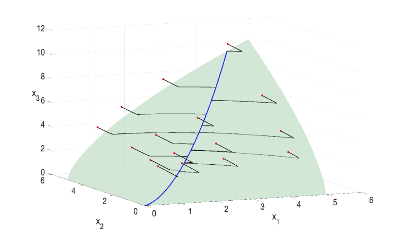
Figure 2: Sample trajectories of (4.6) with initial conditions specified by red points. Green surface: the critical manifold $S_{0}$. Blue curve: family of equilibria $T_{0}\subset S_{0}$. Parameter set: $\varepsilon=0.01$, $k_{1}=1.0$, $k_{2}=0.4$, $k_{-1}=0.5$, $k_{-2}=0.7$.

We may now compute $\phi_{1}$ using (2.20) and (2.23), choosing $X_{1}=0$ for convenience. We find

$$\phi_{1}(\xi) =N_{0}(\xi)Y_{1}(\xi)$$

$$=-N_{0}(\xi)n_{0}(\xi)^{-1}(N_{0}(\xi)^{*}N_{0}(\xi))^{-1}N_{0}(\xi)^{*}(1-P_{0}(\xi))F_{1}(\phi_{0}(\xi))$$

$$=\begin{pmatrix}-2\\ -2\\ 3\end{pmatrix}\frac{K^{1/3}\left(k_{-2}\xi_{2}^{4}-K^{1/3}k_{2}\xi_{1}^{5}\right)\left(3\xi_{1}\xi_{2}+K^{1/3}(4\xi_{1}^{3}-2\xi_{2}^{3})\right)}{k_{1}\xi_{1}^{3}\xi_{2}\left(9\xi_{1}\xi_{2}+4K^{1/3}(\xi_{1}^{3}+\xi_{2}^{3})\right)^{2}}\,.$$ (4.7)

Similarly, the reduced vector field is computed using (2.22):

$$r_{1}(\xi) =(D\phi_{0}(\xi)^{*}D\phi_{0}(\xi))^{-1}D\phi_{0}(\xi)^{*}P_{0}(\xi)(F_{1}(\phi_{0}(\xi)))$$

$$=\frac{K^{1/3}k_{2}\xi_{1}^{5}-k_{-2}\xi_{2}^{4}}{9\xi_{1}\xi_{2}+4K^{1/3}(\xi_{1}^{3}+\xi_{2}^{3})}\begin{pmatrix}-(\xi_{2}^{2}/\xi_{1})(4K^{1/3}\xi_{1}^{2}+5\xi_{2})\\ 4\xi_{2}(\xi_{1}+K^{1/3}\xi_{2}^{2})\end{pmatrix}.$$ (4.8)

This formula agrees with the result in [10]. Note that $r_{1}(\xi)=0$ along the curve $\{K^{1/3}k_{2}\xi_{1}^{5}=k_{-2}\xi_{2}^{4}\}=\phi_{0}^{-1}(T_{0})\subset U_{1}$, corresponding to the curve $T_{0}\subset\mathbb{R}^{3}$ of equilibria of (4.6). Higher-order corrections to this reduced vector field must necessarily also remain trivial along this curve of equilibria. Using (2.22) with $i=2$, (4.7), and (4.8), we find in particular that

$$r_{2}(\xi) =\frac{K^{1/3}(K^{1/3}k_{2}\xi_{1}^{5}-k_{2}\xi_{2}^{4})\tilde{r}_{2}(\xi_{1},\xi_{2})}{k_{1}\xi_{1}^{3}\xi_{2}(9\xi_{1}\xi_{2}+4K^{1/3}(\xi_{1}^{3}+\xi_{2}^{3}))^{3}}\begin{pmatrix}-(4K^{1/3}\xi_{1}^{2}+5\xi_{2})/\xi_{1}\\ 4(\xi_{1}+K^{1/3}\xi_{2}^{2})/\xi_{2}\end{pmatrix},$$

where the auxiliary function $\tilde{r}_{2}(\xi)$ is defined by

$$\tilde{r}_{2}(\xi)=(-4k_{-2}\xi_{2}^{3}+k_{2}\xi_{1}^{2}(-3\xi_{1}+2K^{1/3}\xi_{2}^{2}))(3\xi_{1}\xi_{2}+K^{1/3}(4\xi_{1}^{3}-2\xi_{2}^{3})).$$

Observe that also $r_{2}(\xi)$ vanishes along the curve $\{K^{1/3}k_{2}\xi_{1}^{5}=k_{-2}\xi_{2}^{4}\}=\phi_{0}^{-1}(T_{0})\subset U_{1}$ (which corresponds to the curve of equilibria of the full system).

We finish by investigating the linear fast fibre bundle along $S_{0}^{\varepsilon}$. Here we compute only the first-order correction using (2.45) and (2.47). We find

$$L_{1}(\xi) =((D\phi_{0}(\xi))^{*}D\phi_{0}(\xi))^{-1}(D\phi_{0}(\xi))^{*}P_{0}(\xi)H_{1}(\xi)n_{0}(\xi)^{-1}$$

$$=\frac{K^{1/3}(-4k_{-2}\xi_{2}^{3}+k_{2}\xi_{1}^{2}(-3\xi_{1}+2K^{1/3}\xi_{2}^{2}))}{k_{1}\xi_{1}^{3}\xi_{2}^{3}(9\xi_{1}\xi_{2}+4K^{1/3}(\xi_{1}^{3}+\xi_{2}^{3}))^{2}}\begin{pmatrix}(1/\xi_{1})(4K^{1/3}\xi_{1}^{2}+5\xi_{2})\\ -(4/\xi_{2})(\xi_{1}+K^{1/3}\xi_{2}^{2})\end{pmatrix},$$

from which it follows that the first-order correction of the parametrisation $N_{0}(\xi)$ of the fast fibres is given by $\varepsilon N_{1}(\xi)=\varepsilon D\phi_{0}(\xi)L_{1}(\xi)$ (selecting $M_{1}=0$ for convenience).

Remark 4.4.

We performed the calculations of $r_{1},\phi_{1},r_{2},\phi_{2}$, and $L_{1}$ in Mathematica. The corresponding Mathematica notebook has been uploaded to https://github.com/ianlizarraga/ParametrisationMethod. We also included alternative calculations using the CSP method [23, 24, 26]. $\triangle$

4.2 Three-timescale reaction network.

In this section we study a modified version of a three-species reaction-kinetics model due to Valorani et. al. [34]. The model describes the three reactions

$$X_{1} \overset{k_{1}^{f}}{\underset{k_{1}^{b}}{\rightleftharpoons}}2X_{2}$$

$$X_{1}+X_{2} \overset{k_{2}^{f}}{\underset{k_{2}^{b}}{\rightleftharpoons}}X_{3}$$

$$X_{2}+X_{3} \overset{k_{3}^{f}}{\underset{k_{3}^{b}}{\rightleftharpoons}}X_{1}$$

by means of the two-parameter family of differential equations

$$\begin{pmatrix}x_{1}^{\prime}\\ x_{2}^{\prime}\\ x_{3}^{\prime}\end{pmatrix} =\begin{pmatrix}-1\\ 2\\ 0\end{pmatrix}(x_{1}-x_{2}^{2})+\varepsilon\begin{pmatrix}-1\\ -1\\ 1\end{pmatrix}(x_{1}x_{2}-x_{3})+\delta\begin{pmatrix}1\\ -1\\ -1\end{pmatrix}(x_{2}x_{3}-x_{1})$$ (4.9)

$$=F_{0}(x)+\varepsilon F_{1}(x)+\delta F_{2}(x)\,.$$

Here, $x_{1},x_{2},x_{3}\geq 0$, while $\varepsilon\ll 1$ and $\delta\ll 1$ are two small parameters.

Remark 4.5.

Valorani et. al. focused their analysis on a rescaled variant of (4.9), and used the CSP method to numerically approximate a one-dimensional attracting slow manifold for a parameter set equivalent to $(\varepsilon,\delta)=(0.2,0.002)$. They also gave numerical evidence of an intermediate relaxation onto a two-dimensional surface. In [26] a two-timescale subfamily of (4.9) (equivalent to choosing $\varepsilon=0.2$ fixed and letting $\delta$ vary) was analysed from the point of view of GSPT, and formulas for the first-order corrections of the one-dimensional slow manifold and its fast fibres were derived using the CSP method. $\triangle$

In the following analysis, we choose $\delta=\bar{\delta}\varepsilon^{2}=O(\varepsilon^{2})$ and let $\varepsilon$ vary. This renders the system in the form (4.1) with just one independent small parameter. We show how the parametrisation method algorithmically uncovers genuine three-timescale dynamics (i.e., a nested structure of slow and infra-slow invariant manifolds). Such three-timescale dynamics is also suggested by the numerical integration shown in Figure 3. Because our reaction network is entirely hypothetical, we are free to consider other possible relations between $\varepsilon$ and $\delta$ later.

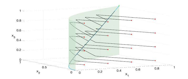
Figure 3: Sample trajectories of (4.9) with initial conditions specified by red points. Green surface: the critical manifold $S_{0}$. Blue curve: the manifold $T_{0}\subset S_{0}$. Green point: stable node at $(1,1,1)$. Parameter set: $\varepsilon=10^{-2}$, $\delta=10^{-4}$.

We start our analysis by noting that our system admits a two-dimensional critical manifold

$$S_{0}=\{(x_{1},x_{2},x_{3}):x_{1}=x_{2}^{2},\,x_{2}>0,\,x_{3}>0\}$$

of equilibrium points of $F_{0}$. This $S_{0}$ admits a smooth parametrisation

$$\phi^{(0)}_{0}(\xi) =\begin{pmatrix}\xi_{1}^{2}\\ \xi_{1}\\ \xi_{2}\end{pmatrix},$$

where $\xi=(\xi_{1},\xi_{2})$ are local coordinates on a chart $U_{1}=\{(\xi_{1},\xi_{2}):\xi_{1},\xi_{2}>0\}\subset\mathbb{R}^{2}$. Note that in this example we use superscripts, in anticipation of finding a nontrivial infra-slow manifold. Recalling Remark 2.7, we also note that the fast fibre bundle along $S_{0}$ is spanned by

$$N^{(0)}_{0}(\xi) =\begin{pmatrix}-1\\ 2\\ 0\end{pmatrix}\,.$$

The first-order corrections $\phi^{(0)}_{1}$ and $r^{(1)}_{1}$ are computed in an identical manner to the previous example; selecting $X_{1}=0$ for convenience, and using (2.22)–(2.23), we find

$$\phi^{(0)}_{1}(\xi) =N^{(0)}_{0}(\xi)Y_{1}(\xi)$$

$$=-N_{0}(\xi)n_{0}(\xi)^{-1}(N_{0}(\xi)^{*}N_{0}(\xi))^{-1}N_{0}(\xi)^{*}(1-P_{0}(\xi))F_{1}(\phi_{0}(\xi))$$

$$=\frac{1}{(1+4\xi_{1})^{2}}\begin{pmatrix}(\xi_{1}^{3}-\xi_{2})(2\xi_{1}-1)\\ -2(\xi_{1}^{3}-\xi_{2})(2\xi_{1}-1)\\ 0\end{pmatrix}\,,$$ (4.10)

and

$$r^{(1)}_{1}(\xi) =(D\phi^{(0)}_{0}(\xi)^{*}D\phi^{(0)}_{0}(\xi))^{-1}D\phi_{0}^{(0)}(\xi)^{*}P_{0}(\xi)(F_{1}(\phi^{(0)}_{0}(\xi)))$$

$$=\begin{pmatrix}\frac{-3}{1+4\xi_{1}}(\xi_{1}^{3}-\xi_{2})\\ \xi_{1}^{3}-\xi_{2}\end{pmatrix}=\begin{pmatrix}-\frac{3}{1+4\xi_{1}}\\ 1\end{pmatrix}(\xi_{1}^{3}-\xi_{2})\,.$$ (4.11)

Note that $r^{(1)}_{1}(\xi)$ admits a factorisation as in Remark 2.2.

Similarly, we use (2.47) to compute the first-order correction of the fast fibres. We find

$$L_{1}(\xi) =\begin{pmatrix}-\frac{3\xi_{1}(1-2\xi_{1})}{(1+4\xi_{1})^{2}}\\ \frac{\xi_{1}(1-2\xi_{1})}{1+4\xi_{1}}\end{pmatrix}.$$

Now note that $r^{(1)}_{1}:U_{1}\to\mathbb{R}^{2}$ admits a curve of equilibria defined by

$$S_{1}=\{\xi_{2}=\xi_{1}^{3}\}=\left(\phi_{0}^{(0)}\right)^{-1}(\{F_{0}=F_{1}=0\})\subset U_{1}\,.$$

As an embedding for $S_{1}$ let us choose $\phi^{(1)}_{0}:U_{2}=\{\eta>0\}\to\mathbb{R}$ defined by

$$\phi^{(1)}_{0}(\eta) =\begin{pmatrix}\eta\\ \eta^{3}\end{pmatrix}\,.$$

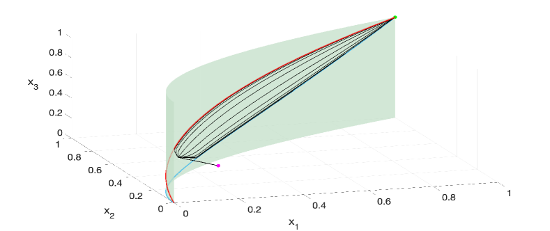
Figure 4: Parameter sweep of (4.9) along the line $(\varepsilon,\delta)=(\varepsilon,(10^{-2}-\varepsilon)+10^{-4})$ for $\varepsilon\in[10^{-4},10^{-2}]$, with initial condition $(0.2,0.2,0.2)$ (magenta point). Green surface is a portion of $S_{0}=\{(x_{2}^{2},x_{2},x_{3}):x_{2}>0,\,x_{3}>0\}$, blue curve is $\{(x_{2}^{2},x_{2},x_{2}^{3}):x_{2}>0\}$, red curve is $\{(x_{2}^{2},x_{2},x_{2}):x_{2}>0\}$. Green point: stable node at $(1,1,1)$.

Using (4.11) and Remark 2.7, we find that the fast fibre bundle along $S_{1}$ is spanned by

$$N^{(1)}_{0}(\xi)=\begin{pmatrix}-\frac{3}{1+4\xi_{1}}\\ 1\end{pmatrix}.$$

We proceed to compute the $O(\varepsilon^{2})$ flow on $S_{1}^{\varepsilon}$ in the chart $U_{2}$, using (3.1). Proposition 4.1 implies that a nontrivial term $F_{2}$ is required to induce a nontrivial flow along a lower-dimensional invariant manifold. In the present example, one can indeed verify directly from (4.10) and (4.11) that $r^{(1)}_{1}|_{S_{1}}=0$ and $\phi^{(0)}_{1}|_{S_{1}}=0$; it follows by (3.1) that $F_{2}\neq 0$ is a necessary condition for $r^{(2)}_{2}\neq 0$. From our formulas for $D\phi^{(0)}_{0},\,D\phi^{(1)}_{0},\,N^{(0)}_{0},$ and $N^{(1)}_{0}$, we obtain that the auxiliary projections defined in (3.2) are given by

$$\tilde{P}_{0}^{(0)}(\xi) =\begin{pmatrix}\frac{2}{1+4\xi_{1}}&\frac{1}{1+4\xi_{1}}&0\\ 0&0&1\end{pmatrix}\,,$$

$$\tilde{P}_{0}^{(1)}(\eta) =\frac{1}{1+4\eta+9\eta^{2}}\begin{pmatrix}1+4\eta&3\end{pmatrix}.$$

By (3.1), we therefore have, denoting $\xi=\phi_{0}^{(1)}(\eta)$,

$$r^{(2)}_{2}(\eta) =\tilde{P}_{0}^{(1)}(\eta)\tilde{P}_{0}^{(0)}(\xi)G_{2}(\xi)$$

$$=\tilde{P}_{0}^{(1)}(\eta)\tilde{P}_{0}^{(0)}(\xi)F_{2}(\xi)$$

$$=\frac{2\bar{\delta}(\eta^{2}-\eta^{4})}{1+4\eta+9\eta^{2}}.$$ (4.12)

For $\bar{\delta}=1$, this expression is identical to the reduced system, written in terms of a parametrisation variable $y$, in [26]. In the latter paper, a two-timescale splitting with a one-dimensional critical manifold $S_{0}=\{(x_{2}^{2},x_{2},x_{2}^{3}):x_{2}>0\}$ was assumed from the start.

We emphasize that the small parameters $\varepsilon$ and $\delta=\bar{\delta}\varepsilon^{2}$ are mutually dependent in the above computations; these computations should therefore be contrasted with the theoretical results in [8] and [22], which are concerned with the persistence of nested invariant manifolds in families of systems with independent small parameters, such as systems of the form (1.4). Our computations illustrate the utility of the parametrisation method to uncover multiple timescale dynamics when the small parameters are interdependent.

Remark 4.6.

After considering the parameter regime $\delta=O(\varepsilon^{2})$, let us now briefly discuss how the computations differ in other parameter regimes. For $\varepsilon=O(\delta^{2})$, an identical analysis to the above reveals a different three-timescale system, in which the one-dimensional critical manifold of the reduced problem is $S_{1}=\{(x_{2}^{2},x_{2},x_{2})\,:\,x_{2}>0\}$. Varying $\varepsilon$ and $\delta$ simultaneously along a curve in parameter space connecting the regions $\varepsilon\ll\delta\ll 1$ and $\delta\ll\varepsilon\ll 1$, we can identify these two distinct three-timescale systems as limiting cases of a one-parameter family of two-timescale systems; see Fig. 4. Numerical integration suggests that in the intermediate regime $\varepsilon\approx\delta$, trajectories near $S_{0}$ still relax onto a one-dimensional curve. This relaxation corresponds to the approach of the trajectories to the stable node at $(1,1,1)$ along a weak eigendirection. The Jacobian evaluated at $(1,1,1)$ is

$$DF(1,1,1) =\begin{pmatrix}-\varepsilon-\delta-1&-\varepsilon+\delta+2&\varepsilon+\delta\\ -\varepsilon+\delta+2&-\varepsilon-\delta-4&\varepsilon-\delta\\ \varepsilon+\delta&\varepsilon-\delta&-\varepsilon-\delta\end{pmatrix}\,.$$ (4.13)

Sylvester’s criterion verifies that the equilibrium point is indeed a stable node for all $\varepsilon,\delta>0$. The corresponding relaxation does not imply the existence of a third (hidden) timescale though, since $r^{(1)}_{1}$ now does not admit a curve of equilibria. $\triangle$

5 Concluding remarks

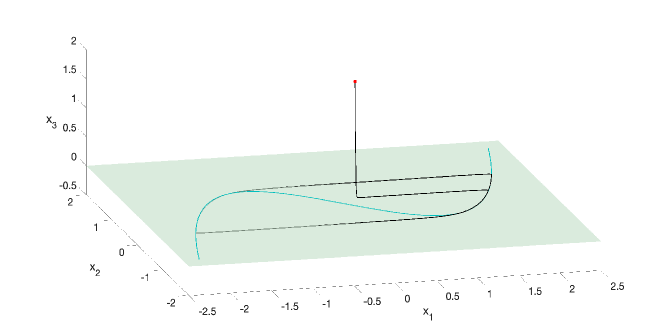
Figure 5: Sample trajectory of (5.1) with $\varepsilon=0.01$ and initial condition $(0.2,0.2,2)$ (red point). Critical manifold $S_{0}=\{x_{3}=0\}$ depicted by green surface; infra-slow critical manifold $S_{1}=\{(x_{1},x_{1}^{3}/3-x_{1},0):x_{1}\in\mathbb{R}\}$ depicted by teal curve.

We have described a novel method to approximate slow manifolds and fast fibre bundles in multiple timescale systems of the general form (1.1) in the spirit of the parametrisation method of Cabré, Fontich and de la Llave et. al. [3, 4, 5, 18]. The power of our method lies in its top-down approach: after computing a smoothly embedded slow manifold $S_{0}^{\varepsilon}$, we can algorithmically uncover and approximate its nested infra-slow manifolds and fast fibres. We emphasize that no a priori knowledge of the ultimate attractor state(s) or the number of disparate timescales is needed to apply the method.

We highlight two important applications of the parametrisation method in this paper: we study the phenomenon of hidden timescales, that can arise in general singularly perturbed systems, and we show how the method can uncover multiple timescale dynamics in systems with dependent small parameters. Both applications lie beyond the current multiple timescale framework introduced by Cardin & Teixeira in [8], and we conclude that systems of the form (1.4) may be too restrictive for the study of general multiple timescale dynamical systems. Building on the important first results in [8], we suggest a (coordinate-independent) geometric definition of a multiple timescale system in our Definition 3.1. The theory for the corresponding nested invariant manifolds in this general context merits further investigation.

One of our goals was to demonstrate the practical implementation of our parametrisation method. Our examples were limited to second-order corrections of the slow manifolds and first-order corrections of the fast fibres, computed symbolically with Mathematica. We anticipate that naive symbolic calculations to obtain higher-order corrections will become unwieldy, since the cost of computing the derivatives in the definitions of $G_{i}$ and $H_{i}$—see (2.8) and (2.45)—grows quickly. For more complex problems, we suggest pairing the parametrisation method with automatic differentiation algorithms [16] to handle this inefficiency. Automatic differentiation has been previously adapted to the parametrisation method to efficiently approximate invariant manifolds of fixed points [18] and isochrons of limit cycles [20].

In this paper we focused on the case of nested normally hyperbolic invariant manifolds. When the nested manifolds are attracting, the long-term behavior of typical trajectories is governed by the dynamics on the slowest timescale. More complicated behavior can occur in general, including switching between several regimes of dynamical timescales as observed in, for example, relaxation oscillations. These more complicated transitions can arise due to possible loss of normal hyperbolicity at some ‘level’ of the nesting, which may not at all be apparent from the general form (1.1). The following embedded Van der Pol system illustrates some of the complications that can occur:

$$x_{1}^{\prime} =\varepsilon(x_{2}+x_{1}-x_{1}^{3}/3)$$

$$x_{2}^{\prime} =-\varepsilon x_{3}$$ (5.1)

$$x_{3}^{\prime} =-x_{3}+\varepsilon x_{1}.$$

This system admits a critical manifold $S_{0}=\{x_{3}=0\}$, and we emphasize that the critical manifold at this ‘top’ level is normally hyperbolic attracting. For $0<\varepsilon\ll 1$, typical trajectories in fact approach a hidden relaxation oscillation within $S_{0}^{\varepsilon}=\{x_{3}=\varepsilon x_{1}+O(\varepsilon^{2})\}$, connecting the slow and the (hidden) infra-slow timescales (see Fig. 5).

We suggest that similar scenarios can arise in chemical reaction networks: a subset of fast precursors is rapidly extinguished, after which the system settles onto a low-dimensional attractor which may itself have distinct temporal features. The parametrisation method can be used to identify both the slow and the infra-slow manifolds and fast fibres, away from the fold points where normal hyperbolicity is lost. In general, the parametrisation method may serve as a useful tool, as a more complete theory for the loss of normal hyperbolicity in multiple timescale systems is developed.

Acknowledgement: The authors would like to thank the referees for their valuable feedback. BR is happy to acknowledge the Sydney Mathematical Research Institute for its hospitality and financial support, and the Dutch mathematics cluster NDNS+ for providing travel support. IL and MW would like to acknowledge support through the ARC DP180103022 grant.

References

- [1] U. Alon, An introduction to systems biology: design principles of biological circuits, Chapman & Hall/CRC (2007).
- [2] J.B. Van den Berg, W. Hetebrij and B. Rink The parameterization method for center manifolds, J. Differ. Eq. 53 (2020), pp. 2132 - 2184.
- [3] X. Cabré, E. Fontich and R. De la Llave, The parameterization method for invariant manifolds I: manifolds associated to non-resonant subspaces, Indiana Univ. Math. Journal (2003), pp. 283–328.
- [4] X. Cabré, E. Fontich and R. De la Llave, The parameterization method for invariant manifolds II: regularity with respect to parameters, Indiana Univ. Math. Journal (2003), pp. 329-360.
- [5] X. Cabré, E. Fontich and R. De la Llave, The parameterization method for invariant manifolds III: overview and applications, J. Diff. Eq. 218, 2 (2005), pp. 444-515.
- [6] M. Canadell and A. Haro, A Newton-like Method for Computing Normally Hyperbolic Invariant Tori, in [18], pp. 187-238.
- [7] M. Canadell and A. Haro, Computation of Quasiperiodic Normally Hyperbolic Invariant Tori: Rigorous Results, J. Nonlin. Sci. 27 (2017), pp. 1-36.
- [8] P. Cardin and M. Teixeira, Fenichel Theory for Multiple Time Scale Singular Perturbation Problems, SIADS 16 (2017), pp. 1425–1452.
- [9] J.J. Duistermaat, Bifurcation of periodic solutions near equilibrium points of Hamiltonian systems, Bifurcation theory and applications (Montecatini, 1983), Lecture Notes in Math. 1057, Springer (1984), pp. 57–105.
- [10] E. Feliu, N. Kruff and S. Walcher, Tikhonov-Fenichel reduction for parametrized critical manifolds with applications to chemical reaction networks, J. Nonlinear Sci. 30 (2020), pp. 1355–1380.
- [11] N. Fenichel, Geometric singular perturbation theory for ordinary differential equations, J. Diff. Eq. 31 (1979), pp. 53–98.
- [12] C.W. Gear, T.J. Kaper, I.G. Kevrekidis, and A. Zagaris, Projecting to a Slow Manifold: Singularly Perturbed Systems and Legacy Codes, SIAM J. Appl. Dyn. Syst. 4 (2005) 711–732.
- [13] A. Goeke and S. Walcher, A constructive approach to quasi-steady state reduction, J. Math. Chem., 52 (2014), pp. 2596–2626.
- [14] M. Golubitsky and I. Stewart, The symmetry perspective, Birkhäuser Verlag, Progress in Mathematics 200 (2002).
- [15] A. Gonzalez, A. Jorba, R. de la Llave and J. Villanueva, KAM Theory without action–angle variables, Nonlinearity 18 (2005), pp. 855–895.
- [16] A. Griewank and A. Walther, Evaluating Derivatives: Principles and Techniques of Algorithmic Differentiation, Second Edition, Society for Industrial and Applied Mathematics (2008).
- [17] C. Groothedde and J.D. Mireles James, Parameterization method for unstable manifolds of delay differential equations, J. Computational Dynamics 4, no. 1 & 2 (2017), pp. 21–70.
- [18] A. Haro, M. Canadell, J. Figueras, A. Luque and J. Mondelo, The parameterization method for invariant manifolds, Springer International Publishing (2016).
- [19] R. Heinrich and M. Schauer, Quasi-steady-state approximation in the mathematical modeling of biochemical networks, Math. Biosci. 65 (1983), pp. 155–170.
- [20] G. Huguet and R. de la Llave, Computation of Limit Cycles and Their Isochrons: Fast Algorithms and Their Convergence, SIAM J. Appl. Dyn. Syst. 12 (2013), pp. 1763–1802.
- [21] H.G. Kaper, T.J. Kaper, and A. Zagaris, Geometry of the Computational Singular Perturbation Method, Math. Model. Nat. Phenom. 10 (2015), pp. 16–30.
- [22] N. Kruff and S. Walcher, Coordinate-independent singular perturbation reduction for systems with three time scales, Math Biosci Eng. 16 (5):5062-5091.
- [23] S.H. Lam and D.A. Goussis, The CSP Method for Simplifying Kinetics, Int. J. Chem. Kinetics 26 (1994), pp. 461–486.
- [24] S.H. Lam and D.A. Goussis, Understanding complex chemical kinetics with computational singular perturbation, Symposium (International) on Combustion, 22 (1989), pp. 931–941.
- [25] C.H. Lee and H.G. Othmer, A multi-time-scale analysis of chemical reaction networks: I. Deterministic systems, J. Math. Biol. 60 (2009), pp. 387–450.
- [26] I. Lizarraga and M. Wechselberger, Computational singular perturbation method for nonstandard slow-fast systems, SIAM J. Appl. Dyn. Sys. 19 (2020), pp. 994–1028.
- [27] U. Maas and S.B. Pope, Implementation of simplified chemical kinetics based on intrinsic low- dimensional manifolds, Proceedings of the 24th International Symposium on Combustion (1992), pp. 103–112.
- [28] U. Maas and S.B. Pope, Simplifying Chemical Kinetics: Intrinsic Low-Dimensional Manifolds in Composition Space, Combustion and Flame 88 (1992), pp. 239–264.
- [29] K.D. Mease, Geometry of Computational Singular Perturbations, IFAC Proceedings Volumes 28 (1995), pp. 855–861.
- [30] C. Reinhardt and J.D. Mireles James, Fourier-Taylor parameterization of unstable manifolds for parabolic partial differential equations: Formalism, implementation and rigorous validation, Indagationes Mathematicae 30, no. 1 (2019), pp. 39 –80.
- [31] M. Stiefenhofer, Quasi-steady-state approximation for chemical reaction networks, J. Math. Biol. 36 (1998), pp. 593–609.
- [32] M. Valorani, H. Najm, and D. Goussis, CSP analysis of a transient flame vortex interaction: time scales and manifolds, Combustion and Flame 134 (2003), pp. 35–53.
- [33] M. Valorani and D. Goussis, Explicit time-scale splitting algorithm for stiff problems: auto-ignition of gaseous-mixtures behind a steady shock, J. Comput. Phys. 168 (2001), pp. 1–36.
- [34] M. Valorani, D. Goussis, F. Creta, and H. Najm, Higher order corrections in the approximation of low-dimensional manifolds and the construction of simplified problems with the CSP method, J. Comp. Phys. 209 (2005), pp. 754–786.
- [35] A. Vanderbauwhede, Centre Manifolds, Normal Forms and Elementary Bifurcations, Dynamics Reported 2 (1989), pp. 89–169.
- [36] M. Wechselberger, Geometric singular perturbation theory beyond the standard form, Springer International Publishing (2020).
- [37] A. Zagaris, H.G. Kaper, and T.J. Kaper, Analysis of the Computational Singular Perturbation Reduction Method for Chemical Kinetics, J. Nonlin Sci. 14 (2004), pp. 59–91.
- [38] A. Zagaris, H.G. Kaper, and T.J. Kaper, Fast and Slow Dynamics for the Computational Singular Perturbation Method, Multiscale Model. Simul. 2 (2004), pp. 613–638.