GraphCrop: Subgraph Cropping for Graph Classification

Abstract

We present a new method to regularize graph neural networks (GNNs) for better generalization in graph classification. Observing that the omission of sub-structures does not necessarily change the class label of the whole graph, we develop the GraphCrop (Subgraph Cropping) data augmentation method to simulate the real-world noise of sub-structure omission. In principle, GraphCrop utilizes a node-centric strategy to crop a contiguous subgraph from the original graph while maintaining its connectivity. By preserving the valid structure contexts for graph classification, we encourage GNNs to understand the content of graph structures in a global sense, rather than rely on a few key nodes or edges, which may not always be present. GraphCrop is parameter learning free and easy to implement within existing GNN-based graph classifiers. Qualitatively, GraphCrop expands the existing training set by generating novel and informative augmented graphs, which retain the original graph labels in most cases. Quantitatively, GraphCrop yields significant and consistent gains on multiple standard datasets, and thus enhances the popular GNNs to outperform the baseline methods.

Introduction

Graph classification is a fundamental task on graph data, which aims to predict the class label of an entire graph. The modern tools of choice for this task are graph neural networks (GNNs). Typically, GNNs build node representations from node features and the graph topology via the ‘message passing’ mechanism and then make graph-level predictions by summarizing the node representations through a readout function (Xu et al. 2018), (Sun et al. 2019).

GNNs are capable of making predictions based on complex graph structures, thanks to their advanced representational power. However, the increased representational capacity comes with higher model complexity, which can induce over-fitting and weaken the generalization ability of GNNs. In this case, a trained GNN may capture random error or noise instead of the underlying data distribution (Zhang et al. 2016), which is not what we expect.

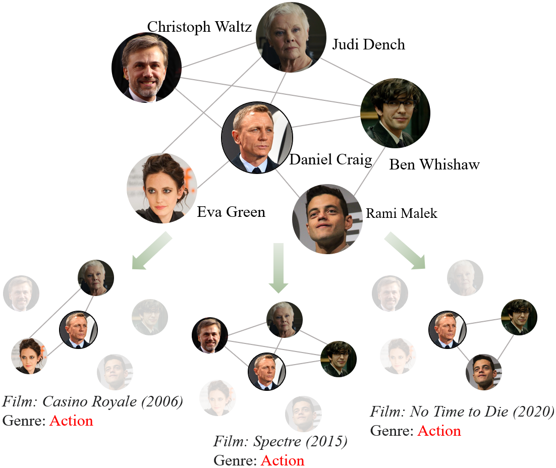
Figure 1: Omission of sub-structures does not change the genre label ‘Action’ of an actor Daniel Craig’s ego-network (Yanardag and Vishwanathan 2015). In the real-world movie collaboration datasets (Yanardag and Vishwanathan 2015), nodes represent actors/actresses, and there is an edge between them if they appear in the same movie. Class labels of graphs are the genres of the movies in which the actors/actresses collaborate.

To combat the over-fitting of neural networks, data augmentation has been demonstrated to be effective in the classification of image data (Perez and Wang 2017). Nevertheless, data augmentation for graph classification remains under-explored, of which a major challenge remains in the high irregularity of graph data. On the one hand, effective data augmentation aims to make significant and diverse modifications to the features while keeping their ground-truth labels unchanged (Xie et al. 2019). On the other hand, how to manipulate a graph without altering its class label is not clear.

In our work, we observe that the omission of partial nodes and edges (sub-structures), does not necessarily change the class label of the whole graph (see Fig. 1). In a scientific collaboration dataset (COLLAB), for example, graphs are ego-networks of researchers, and class labels are the research fields (Yanardag and Vishwanathan 2015). Omission of partial researchers does not necessarily change the research field of the whole graph. In addition, in terms of the real-world noise on graph data, missing partial sub-structures is likely to happen. For instance, to collect an ego-network for a researcher, it is difficult to collect all of his/her collaborators without omission. A satisfactory GNN is expected to classify graphs correctly even in the presence of this type of noise. On the contrary, the collected training graphs may not exhibit enough variance in the absence of sub-structures. As a result, the trained GNN is likely to classify the clean graphs correctly, but fail to recognize the graphs of incomplete structures due to its limited generalization ability.

To address the above issues, we propose a novel data augmentation approach for graph classification, called GraphCrop (Subgraph Cropping), that uses a node-centric strategy to crop a contiguous subgraph from the original graph. GraphCrop can be easily implemented within existing GNNs to achieve better inference performance on graph classification for virtually free. In the training phase, GraphCrop augments a graph within a mini-batch with probability $p$ and keeps it unchanged with probability $1-p$. In the former case, we first select an initial node randomly from the original graph, and then retain the nodes holding the strongest connectivity to the initial node and the edges between them to form the cropped subgraph (see Fig. 2). The number of nodes to retain in the subgraph grows as the size of the original graph, since larger graphs can maintain their original labels while absorbing more noise. To evaluate the connectivity between nodes, we use the diffusion matrix as the metric, which is related to the random walk process over graphs (Pons and Latapy 2005). In this manner, the subgraphs spanning contiguous parts of the original graph are cropped, resulting in the novel and informative samples to expand the existing training set.

Previous work includes DropEdge, a data augmentation technique for the task of node-level predictions, which drops each edge randomly at uniform distribution (Rong et al. 2019). Analogous to it, we refer to the method that drops nodes uniformly as UniNode. Different from both of them, GraphCrop crops a contiguous subgraph which preserves the intact graph structure rather than the individual nodes or edges as DropEdge and UniNode do. GraphCrop ensures the connectivity within the subgraph and conveys valid structural contexts for graph classification. In this fashion, GraphCrop encourages GNNs to understand the content of the graph structure in a global sense, rather than focusing on a few key nodes or edges, which may not always be present. Otherwise, if the nodes or edges are removed uniformly at random, the original structural features may no longer be maintained with the broken topological characteristics. We demonstrate the advantages of GraphCrop empirically.

We evaluate GraphCrop on the graph classification task using the standard chemical (Dobson and Doig 2003) and social (Yanardag and Vishwanathan 2015) datasets. Qualitatively, GraphCrop generates novel augmented graphs, which simulate the real-world noise of sub-structure omission, and preserves the original class labels in most cases (see Fig. 5). Quantitatively, we observe the improvements in test accuracy of graph classification for GNN models trained with GraphCrop. The improvements are higher than those given by the data augmentation designed for other tasks (Rong et al. 2019). Overall, GraphCrop improves the performance of the popular GIN (Xu et al. 2018) and EigenPool (Ma et al. 2019) by a significant margin, and enhances them to outperform the baseline methods.

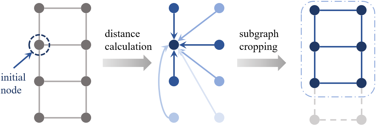
Figure 2: Pipeline of GraphCrop. In the middle column, the connectivity from different nodes to the initial node (in the darkest color) is positively related to their color shades.

Related Work

Graph Classification. Early solutions to graph classification include graph kernels. The pioneering work (Haussler 1999) decomposes graphs into small subgraphs and computes kernel functions based on their pair-wise similarities. Subsequent work proposes various subgraphs, such as paths (Borgwardt and Kriegel 2005), and subtrees (Shervashidze et al. 2009), (Neumann et al. 2016). We refer readers to (Nikolentzos, Siglidis, and Vazirgiannis 2019), (Kriege, Johansson, and Morris 2020) for a general overview. More recently, many efforts have been made to design graph neural networks (GNNs) for graph classification (Scarselli et al. 2008), (Li et al. 2015), (Niepert, Ahmed, and Kutzkov 2016), (Gilmer et al. 2017), (Ying et al. 2018), (Zhang et al. 2018), (Xu et al. 2018). These work focuses on developing GNN architectures of higher complexity to improve their fitting capacity. In contrast, our framework is orthogonal to them in the sense that we propose a new data augmentation method that enhances a GNN model by generating novel and informative augmented graphs for training. As far as we know, we are the first to develop a data augmentation approach for graph classification.

Data Augmentation. Data augmentation plays a central role in training neural networks. It only operates on the input data, without changing the model architecture, but improves the performance significantly. For example, in image classification, strategies such as horizontal flips, random erasing (Zhong et al. 2017), Hide-and-Seek (Singh et al. 2018), and Cutout (DeVries and Taylor 2017) have been shown to improve performance. On graph data, (Wang et al. 2020) proposes NodeAug to augment and utilize the unlabeled nodes in the task of semi-supervised node classification. DropEdge (Rong et al. 2019) removes edges uniformly as data augmentation for node classification. For graph classification, DropEdge is not effective since it tends to break the graph structural properties. Different from it, we crop the contiguous subgraphs from the original graph to generate novel and valid augmented graphs, which simulate the real-world noise of sub-structure omission.

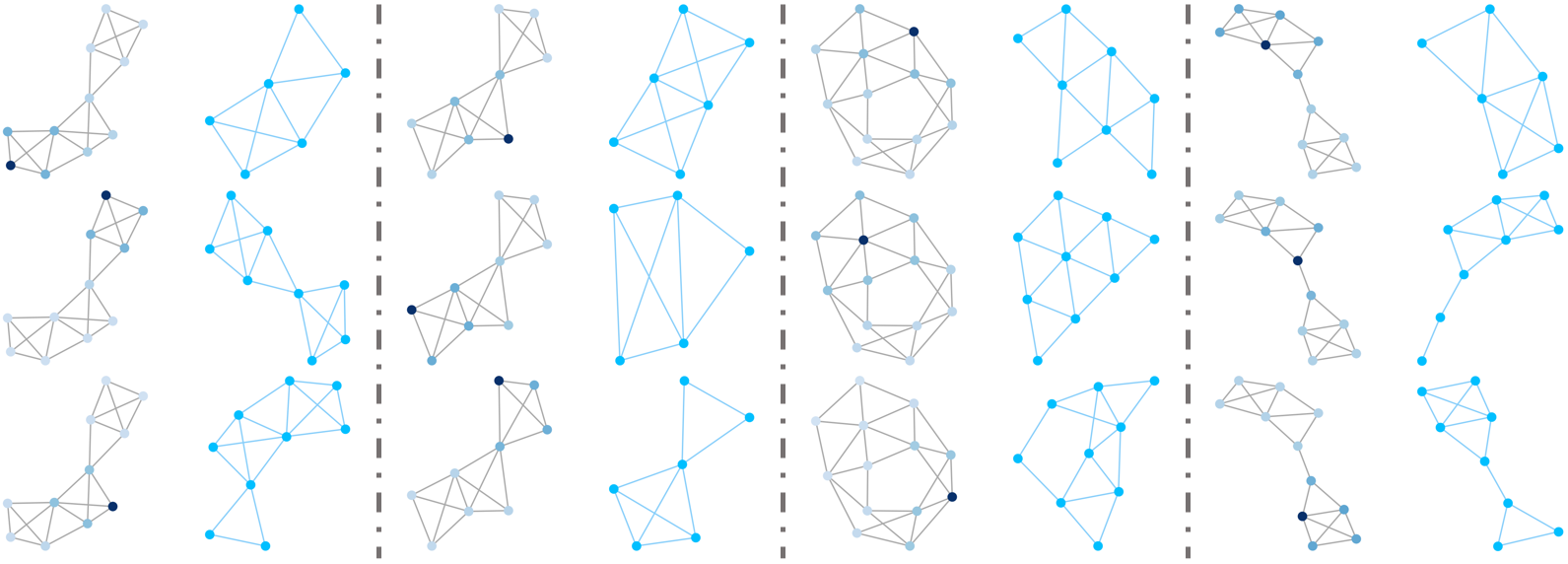
Figure 3: Example subgraphs that GraphCrop obtains from the PROTEINS dataset. The original graphs are in the odd-numbered columns, while the corresponding cropped subgraphs are on their right hand side. The connectivity from different nodes to the initially selected node (in the darkest color) is positively related to their color shades.

Methodology

In this section, we describe the details of our GraphCrop (Subgraph Cropping) data augmentation method. At each training step, GraphCrop augments a graph $G$ in the mini-batch with probability $p$, while keeping $G$ unchanged with probability $1-p$. In this process, graph neural networks (GNNs) are exposed to novel and miscellaneous graphs randomly cropped from the original ones.

Background and Motivation

A graph $G$ consists of a set of nodes $\mathcal{V}$ and a set of edges $\mathcal{E}$. Graph classification aims to learn a mapping function that maps every graph to a predicted class label. Graph neural networks are the state-of-the-art solution for graph classification thanks to their advanced representational capacity. However, the increased representational power also comes with a higher probability of over-fitting, leading to poor generalization. In order to combat the potential for over-fitting, we propose a data augmentation method named GraphCrop to regularize GNNs for better inference performance.

GraphCrop crops a subgraph $\hat{G}$ from $G$ and feeds $\hat{G}$ to GNNs for training. The main motivation of GraphCrop is that the omission of partial nodes and edges (sub-structure) does not necessarily alter the class label of $G$. We visualize an example in Fig. 1 from the movie collaboration datasets, such as IMDB-B, where the graphs are ego-networks of actors/actresses and the class labels are the genre of the movies in which the actors/actresses collaborate (Yanardag and Vishwanathan 2015). The subgraphs of the original ego-network correspond to the real-world movies belonging to the ground truth genre ‘Action’, inferring that the graph label does not change given the omission of some sub-structures. We have similar observations in other kinds of graphs, such as the scientific collaboration datasets (COLLAB) and online discussion community datasets (REDDIT-B) (Yanardag and Vishwanathan 2015). In the former one, for example, graphs are researchers’ ego-networks and labels are their research fields. Omission of partial researchers does not necessarily alter the research fields of the whole graph. Besides, in chemical datasets, prior research has observed that chemical graphs in the same class share common subgraphs (Pržulj 2007), implying the existence of unnecessary sub-structures for categorizing graphs.

In terms of the real-world noise on graph data, missing a partial sub-structure of a graph is likely to happen. For instance, to collect an ego-network for a researcher, it is difficult to collect all of his/her collaborators without omission. For humans, this omission can be negligible because it does not break the connectivity and the topological characteristics of the whole graph. And for GNNs, it is desirable that the models classify graphs correctly invariant to this kind of noise. However, the collected training graphs may exhibit limited variance in the omission of sub-structures. As a result, the learned GNN is likely to work well on the graphs without omission, but fail to recognize the graphs of incomplete structures. We aim to simulate the absence of sub-structures in practice to expand the existing training set. In order to achieve it, we need to maintain connectivity and topological characteristics while conducting subgraph cropping.

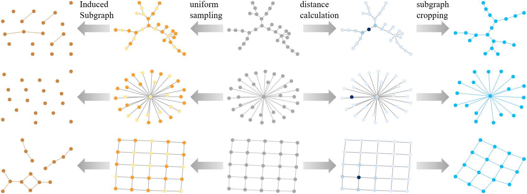
Figure 4: GraphCrop retrieves the subgraphs (fifth column) maintaining the topology characteristics of original graphs (third column). On the other hand, the subgraphs given by UniNode (first column) do not have the original structural property. In column 2, the sampled nodes are in darker colors. In column 4, the nodes’ color shades are positively related to their connectivity to the initially selected node (in the darkest color).

Subgraph Cropping

When cropping a subgraph from the original graph $G$, we need to decide what nodes and edges to retain. We design our GraphCrop method as the following steps:

1. We select a node $v$ (the initial one) uniformly at random from the set of all nodes in $\mathcal{V}$;

2. We evaluate the connectivity from the nodes in $\mathcal{V}_{i}$ to $v$;

3. We select the $\lceil\rho\#\mathcal{V}\rceil$ nodes in $\mathcal{V}$ with the highest connectivity to $v$ and all the edges between them to form the subgraph, where $\rho\in[0,1]$ is a hyper-parameter to adjust the size of the cropped subgraph.

We visualize this pipeline in Fig. 2. Since large graphs have more nodes than small ones, they can absorb more noise while maintaining their ground-truth label. To compensate, we vary the number of nodes in the subgraph by $\lceil\rho\#\mathcal{V}\rceil$. To fulfill step (2), we need to use a metric to evaluate the connectivity between nodes. A simple metric is the length of the shortest paths (Johnson 1973). However, this metric does not necessarily change when connections (paths) between nodes increase, and thus it does not reflect the connectivity effectively. In our work, we utilize the diffusion matrix to measure the connectivity (Fouss et al. 2012):

$$\mathbf{S}=\sum_{k=0}^{\infty}\Theta_{k}\mathbf{T}^{k},$$ (1)

where $\mathbf{T}$ is the generalized transition matrix and $\Theta_{k}$ is the weighting coefficient which determines the ratio of global-local information. Personalized PageRank (PPR) (Page et al. 1999) and heat kernels (Kondor and Lafferty 2002) are two popular instantiations of graph diffusion. Given an adjacency matrix $\mathbf{A}$, and a diagonal degree matrix $\mathbf{D}$, PPR and heat diffusion are defined by setting $\mathbf{A}\mathbf{D}^{-1}$, and $\theta_{k}=\alpha(1-\alpha)^{k}$ and $\theta_{k}=e^{-t}$ respectively, where $\alpha$ denotes teleport probability in a random work and $t$ is diffusion time (Klicpera, Weißenberger, and Günnemann 2019). The closed-form solution to the PPR diffusion is formulated as (Hassani and Khasahmadi 2020):

$$\mathbf{S}^{\text{PPR}}=\alpha(\mathbf{I}-(1-\alpha)\mathbf{D}^{-1/2}\mathbf{A}\mathbf{D}^{-1/2})^{-1},\\$$ (2)

where $\mathbf{I}$ is the identity matrix.

Graph diffusion is related to the random walk process (Pons and Latapy 2005). With $\mathbf{T}=\mathbf{A}\mathbf{D}^{-1}$, $T^{k}_{ij}$ is the probability that a random walk goes from $j$ to $i$ in $k$ steps. A large $k$ achieves a sufficiently long random walk to gather enough information about the topology of the graph. $\mathbf{S}$, as the weighted sum of $\mathbf{T}^{k}$ of different $k$, captures both the local and global connectivity information between nodes. Prior research (Klicpera, Weißenberger, and Günnemann 2019) validates that the graph learning can benefit from the connectivity retrieved by graph diffusion.

GraphCrop can be easily performed on the CPU during data loading. By implementing this operation on the CPU in parallel with the main GPU training task, we can hide its computation and obtain performance improvements virtually for free. Moreover, graph diffusion can be computed once during the pre-processing stage. Existing techniques such as fast approximation and sparsification methods can improve its efficiency (Klicpera, Weißenberger, and Günnemann 2019). We visualize examples of cropped subgraphs in Fig. 3.

Discussion

To augment the graph data, previous research proposes DropEdge (Rong et al. 2019) for node classification, which drops edges uniformly without removing nodes. Similar to it, we name the method to uniformly remove the nodes as UniNode, as visualized in Fig. 4. The main distinction between GraphCrop and the above two methods is that we retain contiguous subgraphs rather than individual nodes, as demonstrated in Fig. 3 and 4. With GraphCrop, the nodes in the cropped subgraphs are connected strongly and the intact topology in the subgraphs is maintained. This is motivated by the discovery from prior research that the subgraphs of strong connectivity contain rich features for recognizing the full graph (Zeng et al. 2019). Hence, the subgraphs convey the intact and valid structural context for graph classification. In this way, GraphCrop forces GNNs to understand the content of the graph structures in a global sense, rather than focusing on a few key nodes, which may not always be present. Otherwise, if the nodes are selected randomly at uniform distribution, as shown in Fig. 4, the topology characteristics of the original graph is broken, and the original structural features are not maintained.

GraphCrop endows every node and edge with non-negligible probability to be sampled, which guarantees that no information is lost through our random data augmentation during training. Overall, GraphCrop simulates the real-world sub-structure omission in the real-world graphs, i.e., it generates graphs that are novel and informative to GNNs. From this vantage, we prepare GNNs for encounters with real-world noise during training, so as to enable GNNs to take more of the graph structural context into consideration when making decisions.

Experiments

Table 1: Statistics of the utilized datasets. $\#$Nodes denotes the average number of nodes per graph, while $\#$Edges denotes the average number of edges per graph.

Dataset	$\#$Graphs	$\#$Nodes	$\#$Edges
D$\&$D	1,178	284.32	715.66
ENZYMES	600	32.63	62.14
NCI1	4,110	29.87	32.30
NCI109	4,127	29.68	32.13
PROTEINS	1,113	39.06	72.82
COLLAB	5,000	74.49	2457.78
IMDB-B	1,000	19.77	96.53
IMDB-M	1,500	13.00	65.94
REDDIT-B	2,000	429.63	497.75
REDDIT-5K	4,999	508.52	594.87

Table 2: Test Accuracy (%) of graph classification on chemical datasets. We perform 10-fold cross-validation to evaluate model performance, and report the mean and standard derivations over 10 folds. We highlight best performances in bold.

Method	D$\&$D	ENZYMES	NCI1	NCI109	PROTEINS
GRAPHLET (Shervashidze et al. 2009)	72.1 $\pm$ 3.7	41.4 $\pm$ 5.2	64.3 $\pm$ 2.2	62.5 $\pm$ 2.8	70.1 $\pm$ 4.1
WL (Shervashidze et al. 2011)	73.2 $\pm$ 1.8	53.7 $\pm$ 6.0	76.3 $\pm$ 1.9	75.8 $\pm$ 2.3	72.3 $\pm$ 3.4
GCN (Kipf and Welling 2016)	74.2 $\pm$ 3.1	59.1 $\pm$ 4.7	76.8 $\pm$ 2.1	76.1 $\pm$ 2.2	73.3 $\pm$ 3.6
DGCNN (Zhang et al. 2018)	76.7 $\pm$ 4.1	39.3 $\pm$ 5.9	76.5 $\pm$ 1.9	75.9 $\pm$ 1.7	72.9 $\pm$ 3.5
DiffPool (Ying et al. 2018)	75.2 $\pm$ 3.8	59.7 $\pm$ 5.3	76.8 $\pm$ 2.0	75.5 $\pm$ 1.9	73.6 $\pm$ 3.6
EigenPool (Ma et al. 2019)	75.9 $\pm$ 3.9	62.4 $\pm$ 3.8	78.7 $\pm$ 1.9	77.4 $\pm$ 2.5	74.1 $\pm$ 3.1
GIN (Xu et al. 2018)	75.4 $\pm$ 2.6	60.3 $\pm$ 4.2	79.7 $\pm$ 1.8	78.2 $\pm$ 2.1	73.5 $\pm$ 3.8
GraphCrop + GCN	75.3 $\pm$ 3.0	60.1 $\pm$ 4.2	77.3 $\pm$ 2.1	77.2 $\pm$ 2.2	74.0 $\pm$ 3.5
GraphCrop + EigenPool	77.3 $\pm$ 3.2	63.6 $\pm$ 3.6	79.6 $\pm$ 2.0	78.5 $\pm$ 2.3	74.9 $\pm$ 3.3
GraphCrop + GIN	76.6 $\pm$ 2.7	60.9 $\pm$ 3.1	80.9 $\pm$ 1.9	79.5 $\pm$ 2.2	74.1 $\pm$ 3.5

Table 3: Test Accuracy (%) of graph classification on social datasets. We perform 10-fold cross-validation to evaluate model performance, and report the mean and standard derivations over 10 folds. We highlight best performances in bold.

Method	COLLAB	IMDB-B	IMDB-M	REDDIT-B	REDDIT-5K
GRAPHLET (Shervashidze et al. 2009)	61.7 $\pm$ 2.2	54.8 $\pm$ 4.1	42.6 $\pm$ 2.7	62.1 $\pm$ 1.6	36.2 $\pm$ 1.8
WL (Shervashidze et al. 2011)	70.4 $\pm$ 1.8	69.1 $\pm$ 3.5	45.4 $\pm$ 2.9	81.7 $\pm$ 1.7	49.4 $\pm$ 2.1
GCN (Kipf and Welling 2016)	74.3 $\pm$ 2.0	70.3 $\pm$ 3.7	48.2 $\pm$ 3.1	86.6 $\pm$ 1.9	53.7 $\pm$ 1.7
DGCNN (Zhang et al. 2018)	71.1 $\pm$ 1.7	69.2 $\pm$ 2.8	45.6 $\pm$ 3.4	87.6 $\pm$ 2.1	49.8 $\pm$ 1.9
DiffPool (Ying et al. 2018)	68.9 $\pm$ 2.2	68.6 $\pm$ 3.1	45.7 $\pm$ 3.4	89.2 $\pm$ 1.8	53.6 $\pm$ 1.4
EigenPool (Ma et al. 2019)	70.8 $\pm$ 1.9	70.4 $\pm$ 3.3	47.2 $\pm$ 3.0	89.9 $\pm$ 1.9	54.5 $\pm$ 1.7
GIN (Xu et al. 2018)	75.5 $\pm$ 2.3	71.2 $\pm$ 3.9	48.5 $\pm$ 3.3	89.8 $\pm$ 1.9	56.1 $\pm$ 1.6
GraphCrop + GCN	75.1 $\pm$ 2.2	71.3 $\pm$ 3.5	48.8 $\pm$ 3.2	87.1 $\pm$ 1.8	54.6 $\pm$ 1.8
GraphCrop + EigenPool	71.7 $\pm$ 2.1	71.0 $\pm$ 3.1	47.9 $\pm$ 3.1	90.8 $\pm$ 1.8	55.2 $\pm$ 1.8
GraphCrop + GIN	76.9 $\pm$ 2.2	72.9 $\pm$ 3.7	49.6 $\pm$ 3.2	91.0 $\pm$ 1.9	57.7 $\pm$ 1.7

In this section, we first present the graph classification performance of GNN models trained with GraphCrop. Next, we adjust the amount of labeled data to evaluate the generalization of GNNs with and without GraphCrop. Then, we visualize the final-layer graph representations retrieved by GNNs and those augmented by GraphCrop. Finally, we conduct ablation studies to show the influence of different node or edge samplers, as well as the sensitivity of the performance with respect to the hyper-parameters of GraphCrop.

We use the standard benchmark datasets: D$\&$D (Dobson and Doig 2003), ENZYMES (Schomburg et al. 2004), NCI1, NCI109 (Wale, Watson, and Karypis 2008), PROTEINS (Borgwardt et al. 2005), COLLAB, IMDB-B, IMDB-M, REDDIT-B, and REDDIT-5K (Yanardag and Vishwanathan 2015) for evaluation. The former five are chemical datasets, where the nodes have categorical input features. The latter five are social datasets that do not have node features. We follow (Xu et al. 2018), (Zhang et al. 2018) to use node degrees as features. The statistics of these datasets are summarized in Table 1.

We use popular graph classification models as the baselines: GRAPHLET (Shervashidze et al. 2009) and Weisfeiler-Lehman Kernel (WL) are classical graph kernel methods, while GCN (Kipf and Welling 2016), DGCNN (Zhang et al. 2018), DiffPool (Ying et al. 2018), EigenPool (Ma et al. 2019), and GIN (Xu et al. 2018) are the GNNs with state-of-the-art performance in graph classification. In addition, we include the recently proposed data augmentation method designed for node classification, DropEdge (Rong et al. 2019), for comparison.

We use the PPR diffusion to measure connectivity by default. For the hyper-parameters of graph diffusion and baselines, e.g., the number of layers, the optimizer, the learning rate, we set them as suggested by their authors. For the hyper-parameters of our CurGraph, we set the augmentation probability $p=0.5$, and $\rho=0.7$ for the sizes of cropped subgraphs by default.

Table 4: Results of node classification averaged over the 20 random splits of the varied ratio $r$ of labeled examples, in terms of test accuracy (%). We highlight the best performance in bold.

Method	NCI1		PROTEINS		COLLAB
	$r=60\%$	$r=80\%$	$r=60\%$	$r=80\%$	$r=60\%$	$r=80\%$
GCN (Kipf and Welling 2016)	68.4 $\pm$ 2.4	72.9 $\pm$ 2.2	65.8 $\pm$ 4.0	70.1 $\pm$ 3.9	67.7 $\pm$ 2.3	71.2 $\pm$ 2.2
GraphCrop + GCN	71.6 $\pm$ 2.2	74.3 $\pm$ 2.1	69.0 $\pm$ 3.8	71.4 $\pm$ 3.7	70.2 $\pm$ 2.3	72.5 $\pm$ 2.3
GIN (Xu et al. 2018)	71.1 $\pm$ 2.2	75.5 $\pm$ 2.0	65.2 $\pm$ 4.1	69.8 $\pm$ 3.7	68.0 $\pm$ 2.5	71.8 $\pm$ 2.3
GraphCrop + GIN	74.5 $\pm$ 2.0	77.1 $\pm$ 1.9	69.1 $\pm$ 3.8	71.2 $\pm$ 3.6	70.6 $\pm$ 2.4	73.7 $\pm$ 2.2

Graph Classification

We follow (Xu et al. 2018), (Errica et al. 2019) to use the 10-fold cross-validation scheme to calculate the classification performance for a fair comparison. For each training fold, as suggested by (Errica et al. 2019), we conduct an inner holdout technique with a $90\%/10\%$ training/validation split, i.e., we train fifty times on a training fold holding out a random fraction ($10\%$) of the data to perform early stopping. These fifty separate trials are needed to smooth the effect of unfavorable random weight initialization on test performances. The final test fold score is obtained as the mean of these fifty runs.

We report the average and standard deviation of test accuracy across the 10 folds within the cross-validation on the chemical and social datasets in Table 2 and 3 respectively. On the chemical datasets, we observe that GraphCrop improves the test accuracy of EigenPool by 1.8% on D&D, 1.9% on ENZYMES, 1.1% on NCI1, 1.4% on NCI109, 1.1% on PROTEINS respectively. In addition, GraphCrop enhances GIN by 1.6% on D&D, 1.0% on ENZYMES, 1.5% on NCI1, 1.7% on NCI109, 0.8% on PROTEINS, and improves GCN by 1.5% on D&D, 1.7% on ENZYMES, 0.7% on NCI1, 1.4% on NCI109, 1.0% on PROTEINS. On the social datasets, GraphCrop improves GCN by more than 1% on COLLAB, IMDB-B, IMDB-M, and REDDIT-5K. Meanwhile, GraphCrop achieves substantial improvements for EigenPool and GIN on all the social datasets. As a result, CurGraph enhances EigenPool and GIN to outperform all the baseline methods.

Taking a closer look, we observe that the graph kernel methods, GRAPHLET and WL, generally present worse performance than the GNN methods. This demonstrates the stronger fitting capacity of the advanced neural network models. GraphCrop generally achieves higher improvements on EigenPool and GIN than that on GCN. The reason is that EigenPool and GIN are the more advanced GNN models proposed for graph classification than GCN. However, their increased learning power comes with higher risks of over-fitting. Our GraphCrop effectively regularizes them by expanding the training set with the novel and informative augmented graphs, which reduces their over-fitting tendencies successfully.

Training Set Sizing

Over-fitting tends to be more severe when training on smaller datasets. By conducting experiments using a restricted fraction of the available training data, we show that GraphCrop has more significant improvements for smaller training sets. We randomly select $r\in\{60\%,80\%\}$ graphs from the whole set to form the labeled data, with the left graphs being the test graphs, to form a split. For each labeled set, as suggested by (Errica et al. 2019), we conduct an inner holdout technique with a $90\%/10\%$ training/validation split. In other words, we train fifty times on a labeled set holding out a random fraction ($10\%$) of the data to perform early stopping. These fifty separate trials are needed to smooth the effect of unfavorable random weight initialization on test performances. We conduct the experiments on 20 random splits and report the mean and standard derivations over all splits in Table 4. Empirically, GraphCrop enhances the performance of GCN and GIN for different sizes of the training set. In principle, with less labeled nodes, i.e., smaller $r$, our method gives larger accuracy improvements, which demonstrates the necessity of the regularization given by our GraphCrop especially when the labeled data is limited.

Visualization of GraphCrop

In data augmentation, input data is altered while the ground-truth labels are expected to remain unchanged. If graphs are significantly changed, however, the original class labels may no longer be valid. We take a visualization approach to examine whether GraphCrop significantly changes the semantic features of augmented graphs. First, we train a GIN on the NCI109 dataset without augmentation. Then we apply GraphCrop to generate an augmented graph per original graph. These are fed into the GIN along with the original graphs, and we extract the final-layer representations. We visualize these graph representations in Fig. 5 via t-SNE (Van Der Maaten 2014). We find that the resulting latent space representations for augmented graphs closely surround those of the original graphs, which suggests that for the most part, graphs augmented with GraphCrop conserve the labels of their original graphs.

(a) GIN

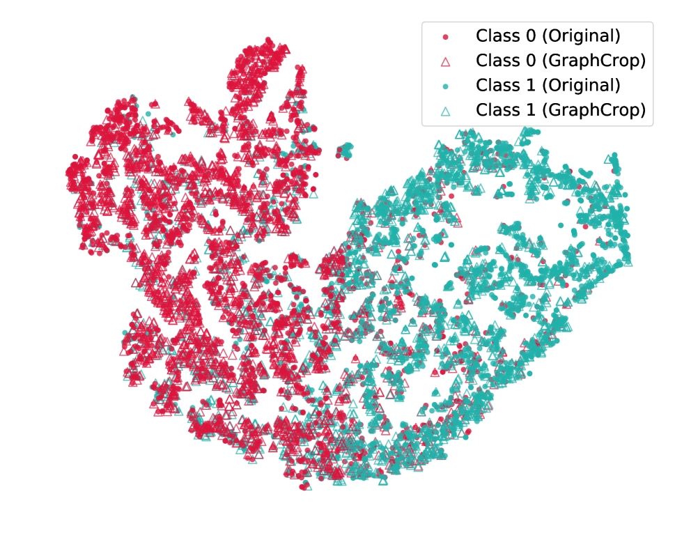
(b) GraphCrop

Figure 5: Augmented graphs (triangles) closely surround original graphs (circles) of the same class (color), suggesting that augmented graphs maintianed their original labels. We visualize the final-layer graph representations of the original and augmented graphs from the NCI109 dataset using t-SNE (Van Der Maaten 2014)

Ablation Study

We conduct a number of ablations to analyze GraphCrop. First, we investigate the effects of the subgraph sampling. Using our GraphCrop method, we can optionally use the shortest path (SP) or heat diffusion to evaluate connectivity in addition to our default PPR diffusion. Moreover, we try another two options for subgraph sampling, of which the first one is to uniformly sample all the nodes to retain in the subgraph (UniNode), as visualized in Fig. 4. The second one is DropEdge (Rong et al. 2019) designed for node classification, which drops edges uniformly without removing nodes. We compare the test accuracy of GIN trained with the above-mentioned subgraph sampling techniques in Table 5. Our GraphCrop with different subgraph sampling methods achieves much better performance than UniNode and DropEdge. The reason is that both UniNode and DropEdge do not guarantee the connectivity between the nodes in the cropped subgraph. They retain individual nodes or edges rather than the contiguous subgraphs as GraphCrop does. As a result, the original graph structural characteristics are difficult to maintain in the cropped subgraph. In contrast, GraphCrop retrieves the subgraphs containing the intact and valid structural context for graph classification. This encourages GNNs to better utilize the global structural context of a graph, rather than relying on the presence of a few key nodes, which may not be present. GraphCrop with SP performs worse than GraphCrop with PPR diffusion, since the shortest path distance does not necessarily change when connections (paths) between nodes increase and thus it does not reflect the connectivity effectively. Empirically, PPR diffusion achieves promising performance.

Table 5: Test Accuracy (%) of graph classification of GIN trained with different subgraph sampling methods.

Method	D&D	NCI109	IMDB-B
UniNode	75.6 $\pm$ 2.4	78.3 $\pm$ 2.1	71.5 $\pm$ 3.9
DropEdge	75.5 $\pm$ 2.6	78.3 $\pm$ 2.2	71.3 $\pm$ 3.7
GraphCrop (SP)	76.1 $\pm$ 2.4	79.2 $\pm$ 2.3	72.5 $\pm$ 3.6
GraphCrop (heat)	76.4 $\pm$ 2.6	79.1 $\pm$ 2.1	72.8 $\pm$ 3.8
GraphCrop (PPR)	76.6 $\pm$ 2.7	79.5 $\pm$ 2.2	72.9 $\pm$ 3.7

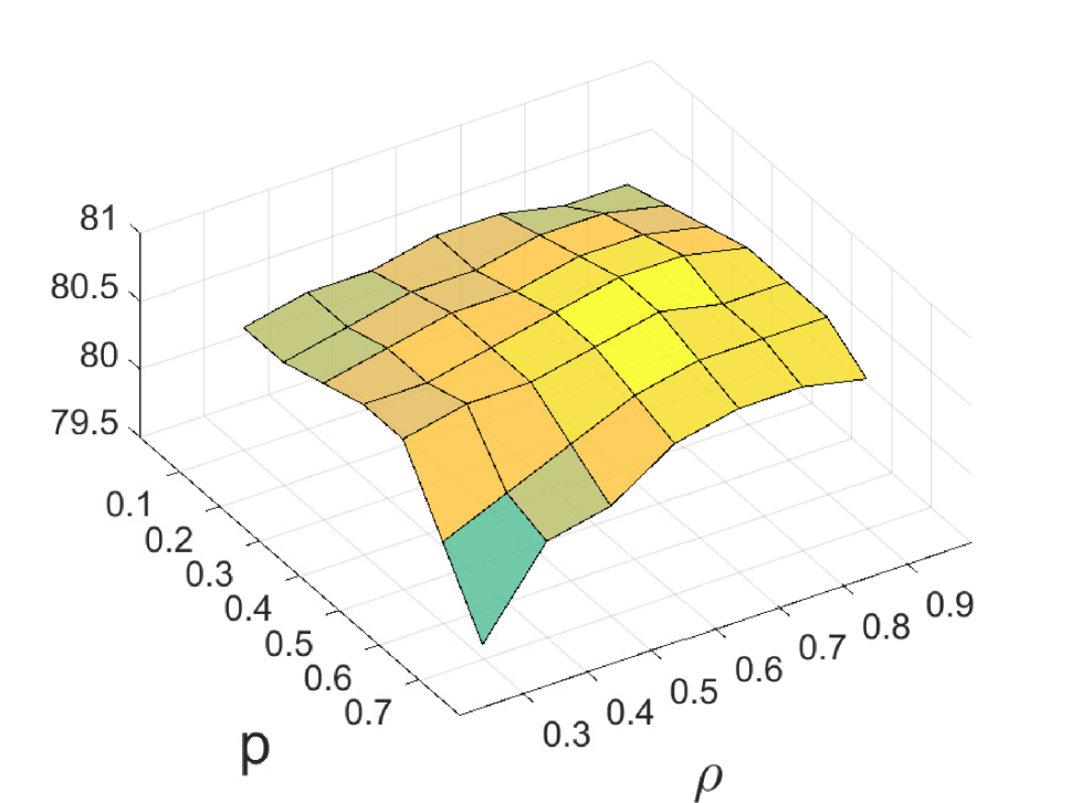
(a) NCI1

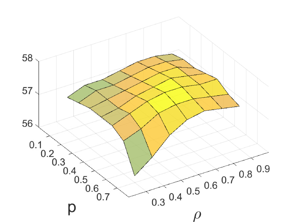
(b) REDDIT-5K

Figure 6: The test accuracy (z-axis) of GIN enhanced by GraphCrop with different hyperparameter values $p$ and $\rho$.

Last but not least, we evaluate how sensitive our GraphCrop is to the selection of hyper-parameter values: $p$ to control the probability of our random data augmentation during training and $\rho$ to adjust the subgraph sizes. As we can see, the performance of GIN with CurGraph is relatively smooth when parameters are within certain ranges. However, extremely large values of $p$ and severely small values of $\rho$ result in low performances, which should be avoided in practice. Moreover, increasing $p$ from 0.1 to 0.5 improves the test accuracy of GIN with GraphCrop, demonstrating that the novel and valid augmented graphs provided by our GraphCrop plays an important role in improving the performance of GNNs.

Conclusion

In this paper, we propose a new data augmentation approach named GraphCrop (Subgraph Cropping) for graph classification. GraphCrop uses a node-centric strategy to crop subgraphs that span the contiguous parts of the original graphs, which hold strong inner connectivity. In principle, it simulates the real-world noise of sub-structure omission to expand the original training set. By training GNNs with GraphCrop, we regularize GNNs to achieve better generalization virtually for free. We conduct the experiments on the standard datasets collected from diverse scenarios. Empirical results show that GraphCrop achieves consistent and substantial improvements for GNN architectures in terms of test accuracy. In future work, we will explore more data augmentation techniques for graph classification and apply them to other tasks requiring graph-level representations.

References

- Borgwardt and Kriegel (2005) Borgwardt, K. M.; and Kriegel, H.-P. 2005. Shortest-path kernels on graphs. In Fifth IEEE international conference on data mining (ICDM’05), 8–pp. IEEE.
- Borgwardt et al. (2005) Borgwardt, K. M.; Ong, C. S.; Schönauer, S.; Vishwanathan, S.; Smola, A. J.; and Kriegel, H.-P. 2005. Protein function prediction via graph kernels. Bioinformatics 21(suppl_1): i47–i56.
- DeVries and Taylor (2017) DeVries, T.; and Taylor, G. W. 2017. Improved Regularization of Convolutional Neural Networks with Cutout. arXiv preprint arXiv:1708.04552 .
- Dobson and Doig (2003) Dobson, P. D.; and Doig, A. J. 2003. Distinguishing enzyme structures from non-enzymes without alignments. Journal of molecular biology 330(4): 771–783.
- Errica et al. (2019) Errica, F.; Podda, M.; Bacciu, D.; and Micheli, A. 2019. A fair comparison of graph neural networks for graph classification. arXiv preprint arXiv:1912.09893 .
- Fouss et al. (2012) Fouss, F.; Francoisse, K.; Yen, L.; Pirotte, A.; and Saerens, M. 2012. An experimental investigation of kernels on graphs for collaborative recommendation and semisupervised classification. Neural networks 31: 53–72.
- Gilmer et al. (2017) Gilmer, J.; Schoenholz, S. S.; Riley, P. F.; Vinyals, O.; and Dahl, G. E. 2017. Neural message passing for quantum chemistry. arXiv preprint arXiv:1704.01212 .
- Hassani and Khasahmadi (2020) Hassani, K.; and Khasahmadi, A. H. 2020. Contrastive Multi-View Representation Learning on Graphs. arXiv preprint arXiv:2006.05582 .
- Haussler (1999) Haussler, D. 1999. Convolution kernels on discrete structures. Technical report, Technical report, Department of Computer Science, University of California ….
- Johnson (1973) Johnson, D. B. 1973. A note on Dijkstra’s shortest path algorithm. Journal of the ACM (JACM) 20(3): 385–388.
- Kipf and Welling (2016) Kipf, T. N.; and Welling, M. 2016. Semi-supervised classification with graph convolutional networks. arXiv preprint arXiv:1609.02907 .
- Klicpera, Weißenberger, and Günnemann (2019) Klicpera, J.; Weißenberger, S.; and Günnemann, S. 2019. Diffusion improves graph learning. In Advances in Neural Information Processing Systems, 13354–13366.
- Kondor and Lafferty (2002) Kondor, R. I.; and Lafferty, J. 2002. Diffusion kernels on graphs and other discrete structures. In Proceedings of the 19th international conference on machine learning, volume 2002, 315–22.
- Kriege, Johansson, and Morris (2020) Kriege, N. M.; Johansson, F. D.; and Morris, C. 2020. A survey on graph kernels. Applied Network Science 5(1): 1–42.
- Li et al. (2015) Li, Y.; Tarlow, D.; Brockschmidt, M.; and Zemel, R. 2015. Gated graph sequence neural networks. arXiv preprint arXiv:1511.05493 .
- Ma et al. (2019) Ma, Y.; Wang, S.; Aggarwal, C. C.; and Tang, J. 2019. Graph convolutional networks with eigenpooling. In Proceedings of the 25th ACM SIGKDD International Conference on Knowledge Discovery & Data Mining, 723–731.
- Neumann et al. (2016) Neumann, M.; Garnett, R.; Bauckhage, C.; and Kersting, K. 2016. Propagation kernels: efficient graph kernels from propagated information. Machine Learning 102(2): 209–245.
- Niepert, Ahmed, and Kutzkov (2016) Niepert, M.; Ahmed, M.; and Kutzkov, K. 2016. Learning convolutional neural networks for graphs. In International conference on machine learning, 2014–2023.
- Nikolentzos, Siglidis, and Vazirgiannis (2019) Nikolentzos, G.; Siglidis, G.; and Vazirgiannis, M. 2019. Graph kernels: A survey. arXiv preprint arXiv:1904.12218 .
- Page et al. (1999) Page, L.; Brin, S.; Motwani, R.; and Winograd, T. 1999. The PageRank citation ranking: Bringing order to the web. Technical report, Stanford InfoLab.
- Perez and Wang (2017) Perez, L.; and Wang, J. 2017. The effectiveness of data augmentation in image classification using deep learning. arXiv preprint arXiv:1712.04621 .
- Pons and Latapy (2005) Pons, P.; and Latapy, M. 2005. Computing communities in large networks using random walks. In International symposium on computer and information sciences, 284–293. Springer.
- Pržulj (2007) Pržulj, N. 2007. Biological network comparison using graphlet degree distribution. Bioinformatics 23(2): e177–e183.
- Rong et al. (2019) Rong, Y.; Huang, W.; Xu, T.; and Huang, J. 2019. Dropedge: Towards deep graph convolutional networks on node classification. In International Conference on Learning Representations.
- Scarselli et al. (2008) Scarselli, F.; Gori, M.; Tsoi, A. C.; Hagenbuchner, M.; and Monfardini, G. 2008. The graph neural network model. IEEE Transactions on Neural Networks 20(1): 61–80.
- Schomburg et al. (2004) Schomburg, I.; Chang, A.; Ebeling, C.; Gremse, M.; Heldt, C.; Huhn, G.; and Schomburg, D. 2004. BRENDA, the enzyme database: updates and major new developments. Nucleic acids research 32(suppl_1): D431–D433.
- Shervashidze et al. (2011) Shervashidze, N.; Schweitzer, P.; Van Leeuwen, E. J.; Mehlhorn, K.; and Borgwardt, K. M. 2011. Weisfeiler-lehman graph kernels. Journal of Machine Learning Research 12(9).
- Shervashidze et al. (2009) Shervashidze, N.; Vishwanathan, S.; Petri, T.; Mehlhorn, K.; and Borgwardt, K. 2009. Efficient graphlet kernels for large graph comparison. In Artificial Intelligence and Statistics, 488–495.
- Singh et al. (2018) Singh, K. K.; Yu, H.; Sarmasi, A.; Pradeep, G.; and Lee, Y. J. 2018. Hide-and-Seek: A Data Augmentation Technique for Weakly-Supervised Localization and Beyond. arXiv preprint arXiv:1811.02545 .
- Sun et al. (2019) Sun, F.-Y.; Hoffmann, J.; Verma, V.; and Tang, J. 2019. Infograph: Unsupervised and semi-supervised graph-level representation learning via mutual information maximization. arXiv preprint arXiv:1908.01000 .
- Van Der Maaten (2014) Van Der Maaten, L. 2014. Accelerating t-SNE using tree-based algorithms. The Journal of Machine Learning Research 15(1): 3221–3245.
- Wale, Watson, and Karypis (2008) Wale, N.; Watson, I. A.; and Karypis, G. 2008. Comparison of descriptor spaces for chemical compound retrieval and classification. Knowledge and Information Systems 14(3): 347–375.
- Wang et al. (2020) Wang, Y.; Wang, W.; Liang, Y.; Cai, Y.; Liu, J.; and Hooi, B. 2020. NodeAug: Semi-Supervised Node Classification with Data Augmentation. In Proceedings of the 26th ACM SIGKDD International Conference on Knowledge Discovery & Data Mining, 207–217.
- Xie et al. (2019) Xie, Q.; Dai, Z.; Hovy, E.; Luong, M.-T.; and Le, Q. V. 2019. Unsupervised data augmentation for consistency training. arXiv preprint arXiv:1904.12848 .
- Xu et al. (2018) Xu, K.; Hu, W.; Leskovec, J.; and Jegelka, S. 2018. How Powerful are Graph Neural Networks? In International Conference on Learning Representations.
- Yanardag and Vishwanathan (2015) Yanardag, P.; and Vishwanathan, S. 2015. Deep graph kernels. In Proceedings of the 21th ACM SIGKDD International Conference on Knowledge Discovery and Data Mining, 1365–1374.
- Ying et al. (2018) Ying, Z.; You, J.; Morris, C.; Ren, X.; Hamilton, W.; and Leskovec, J. 2018. Hierarchical graph representation learning with differentiable pooling. In Advances in neural information processing systems, 4800–4810.
- Zeng et al. (2019) Zeng, H.; Zhou, H.; Srivastava, A.; Kannan, R.; and Prasanna, V. 2019. Accurate, efficient and scalable graph embedding. In 2019 IEEE International Parallel and Distributed Processing Symposium (IPDPS), 462–471. IEEE.
- Zhang et al. (2016) Zhang, C.; Bengio, S.; Hardt, M.; Recht, B.; and Vinyals, O. 2016. Understanding deep learning requires rethinking generalization. arXiv preprint arXiv:1611.03530 .
- Zhang et al. (2018) Zhang, M.; Cui, Z.; Neumann, M.; and Chen, Y. 2018. An end-to-end deep learning architecture for graph classification. In Thirty-Second AAAI Conference on Artificial Intelligence.
- Zhong et al. (2017) Zhong, Z.; Zheng, L.; Kang, G.; Li, S.; and Yang, Y. 2017. Random erasing data augmentation. arXiv preprint arXiv:1708.04896 .