Comment on: “Some quantum aspects of a particle with electric quadrupole moment interacting with an electric field subject to confining potentials”. Int. J. Mod. Phys. A 29 (2014) 1450117

Abstract

We analyze the results obtained from a model consisting of the interaction between the electric quadrupole moment of a moving particle and an electric field. We argue that the system does not support bound states because the motion along the $z$ axis is unbounded. It is shown that the author obtains a wrong bound-state spectrum for the motion in the $x-y$ plane and that the existence of allowed cyclotron frequencies is an artifact of the approach.

In a paper published in this journal Bakke[1] studies the bound states of a quantum-mechanical model given by the interaction between the electric quadrupole of a moving particle and an electric field. In two other models the author adds a harmonic potential and a linear plus harmonic potential. By means of suitable transformations of the time-dependent Schrödinger equation the author derives an eigenvalue equation for the radial part of the wavefunction that can be treated by means of the Frobenius (or power-series) method. In the two cases with radial potentials the power-series method leads to three-term recurrence relations. Suitable truncation of the series yields analytical expressions for the energy eigenvalues and a striking result: the appearance of allowed cyclotron frequencies. The purpose of this Comment is the analysis of the truncation method used by Bakke and its effect on the physical conclusions drawn in his paper.

Upon taking into account the interaction between the electric quadrupole of the moving particle and the electric field the author derives the time-dependent Schrödinger equation

$$i\frac{\partial\psi}{\partial t}=-\frac{1}{2m}\left(\frac{\partial^{2}}{\partial\rho^{2}}+\frac{1}{\rho}\frac{\partial}{\partial\rho}+\frac{1}{\rho^{2}}\frac{\partial^{2}}{\partial\varphi^{2}}+\frac{\partial^{2}}{\partial z^{2}}\right)\psi-\frac{QE_{0}}{\rho}\psi,$$ (1)

in cylindrical coordinates ($0\leq\rho<\infty$, $0\leq\varphi\leq 2\pi$, $-\infty<z<\infty$) and units such that $\hbar=c=1$ (we have recently criticized this kind of nonrigorous choice of suitable units[2]). The meaning of every parameter in this equation is given in the author’s paper[1].

Since the Hamiltonian operator is time-independent and commutes with $\hat{p}_{z}$ and $\hat{L}_{z}$ the author looks for a particular solution of the form

$$\psi(t,\rho,\varphi,z)=e^{-i\mathcal{E}t}e^{il\varphi}e^{ikz}R(\rho),$$ (2)

where $l=0,\pm 1,\pm 2,\ldots$ and $-\infty<k<\infty$. The function $R(\rho)$ satisfies the differential equation

$$R^{\prime\prime}+\frac{1}{\rho}R^{\prime}-\frac{l^{2}}{\rho^{2}}R+\frac{\tilde{Q}E_{0}}{\rho}R+\zeta^{2}R=0,$$ (3)

where $\zeta^{2}=2m\mathcal{E}-k^{2}$ and $\tilde{Q}=2mQ$. After analyzing the behaviour of $R(\rho)$ at infinity the author argues that “Therefore, we can find either scattering states $\left(R\cong e^{i\zeta\rho}\right)$ or bound states $R\cong\left(e^{-\tau\rho}\right)$. Our intention is to obtain bound state solutions, then we consider $\zeta^{2}=-\tau^{2}$”.

It is worth mentioning that the Schrödinger equation discussed above does not have bound-states for any value of $\tilde{Q}E_{0}$ since the motion is unbounded along the $z$ direction (the Hamiltonian operator commutes with $\hat{p}_{z}$). For this reason one introduces the term $e^{ikz}$, and the energy, which depends on $k^{2}/(2m)$, takes all the values $\mathcal{E}\geq\zeta^{2}/(2m)$. To be more specific, we have bound states only if

$$\int\int\int\left|\psi(t,\rho,\varphi,z)\right|^{2}\rho\,d\rho\,d\varphi\,dz<\infty,$$ (4)

as shown in any textbook on quantum mechanics[3, 4]. In all the examples discussed here the improper integral over $z$ is obviously divergent. However, since there is physical interest in the bound states for the motion restricted to the plane $x-y$[3, 4] we will discuss them in what follows.

In the second model the author adds the potential $V(\rho)=\frac{1}{2}m\omega^{2}\rho^{2}$ ($\rho^{2}=x^{2}+y^{2}$) that is clearly unable to bound the motion along the $z$ axis but, as stated above, we will focus on the motion in the $x-y$ plane. By means of the change of variables $\xi=\sqrt{m\omega}\rho$ one obtains the radial eigenvalue equation

$$R^{\prime\prime}+\frac{1}{\xi}R^{\prime}-\frac{l^{2}}{\xi^{2}}R+\frac{\alpha}{\xi}R-\xi^{2}R+\frac{\zeta^{2}}{m\omega}R=0,$$ (5)

where $\alpha=\frac{\tilde{Q}E_{0}}{\sqrt{m\omega}}$.

On writing the solution $R(\xi)$ as

$$R(\xi)=\xi^{|l|}e^{-\frac{\xi^{2}}{2}}\sum_{j=0}^{\infty}a_{j}\xi^{j},$$ (6)

one obtains the three-term recurrence relation

$$a_{j+2} = -\frac{\alpha}{(j+2)(j+1+\theta)}a_{j+1}-\frac{g-2j}{(j+2)(j+1+\theta)}a_{j},$$

$$j = -1,0,1,2\ldots,\;a_{0}=1,\,a_{-1}=0,$$ (7)

where $\theta=2|l|+1$ and $g=\frac{\zeta^{2}}{m\omega}-2-2|l|$.

The author argues as follows: “Bound state solutions correspond to finite solutions, therefore, we can obtain bound state solutions by imposing that the power series expansion (22) or the Heun biconfluent series becomes a polynomial of degree $n$. Through the expression (23), we can see that the power series expansion (22) becomes a polynomial of degree $n$ if we impose the conditions:

$$g=2n\ \mathrm{and}\ a_{n+1}=0,$$ (8)

where $n=1,2,\ldots$.”

It clearly follows from these two conditions that $a_{j}=0$ for all $j>n$; however, the author’s statement is a gross conceptual error because a bound state simply requires that $R(\xi)$ is square integrable:

$$\int_{0}^{\infty}\left|R(\xi)\right|^{2}\xi\,d\xi<\infty,$$ (9)

as shown in any textbook on quantum mechanics[3, 4]. Therefore, the truncation condition may not render all the bound states.

For example, when $n=1$ the first condition yields $g=2$ and one obtains a simple analytical expression for $\mathcal{E}_{1,l}$. The second condition $a_{2}=0$ yields $\alpha=\alpha_{1,l}=\pm\sqrt{4|l|+2}$ and the cyclotron frequency $\omega_{1,l}=\left(\tilde{Q}E_{0}\right)^{2}/(m\alpha_{1,l}^{2})$. From the general case (8) the author derives an analytic expression for $\mathcal{E}_{n,l}$ corresponding to $\omega_{n,l}=\left(\tilde{Q}E_{0}\right)^{2}/(m\alpha_{n,l}^{2})$. Accordingly, he argues as follows: “This means that not all values of the angular frequency $\omega$ are allowed, but some specific values of $\omega$ which depend on the quantum numbers $\{n,l\}$; thus, we label $\omega=\omega_{n,l}$.” Later on he also states that “Hence, we have seen in Eq. (28) that the effects of the Coulomb-like potential induced by the interaction between an electric field and an electric quadrupole moment on the spectrum of energy of the harmonic oscillator corresponds to a change of the energy levels, whose ground state is defined by the quantum number $n=1$ and the angular frequency depends on the quantum numbers $\{n,l\}$. This dependence of the cyclotron frequency on the quantum numbers $\{n,l\}$ means that not all values of the cyclotron frequency are allowed, but some specific values of the harmonic oscillator frequency defined in such a way that the conditions established in Eq. (25) are satisfied and a polynomial solution to the function $H(\xi)$ given in Eq. (22) is achieved.”

Both conclusions are wrong as we shall see in what follows. In the first place, the truncation conditions (8) only yield some rather rare bound states, based on polynomial functions, that occur for some arbitrary particular values of $\alpha$. More precisely, the energy $\mathcal{E}_{n,l}$ obtained by the author comes from an eigenvalue of the differential equation (5) with $\alpha=\alpha_{n,l}$ while any other energy $\mathcal{E}_{n^{\prime},l^{\prime}}$ comes from an eigenvalue of that equation with $\alpha=\alpha_{n^{\prime},l^{\prime}}$; that is to say: those energies are not members of the same spectrum but eigenvalues of two different operators. This fact is obvious for anybody familiar with the exact solutions of any quasi-solvable (or conditionally solvable) model[5, 7, 6] (and references therein).

In order to make the point above clearer we solve the eigenvalue equation (5) for $W=\frac{\zeta^{2}}{m\omega}$ by means of the reliable Rayleigh-Ritz variational method that is well known to yield increasingly accurate upper bounds to all the eigenvalues of the Schrödinger equation[8] (and references therein). For simplicity we choose the basis set of (non-orthogonal) functions $\left\{u_{j}(\xi)=\xi^{|l|+j}e^{-\frac{\xi^{2}}{2}},\;j=0,1,\ldots\right\}$. We verify the accuracy of these results by means of the powerful Riccati-Padé method[9]. To begin with, notice that the eigenvalue equation (5) exhibits bound states for all real values of $l$ and $\alpha$ and not only for the particular values of $\alpha$ considered by the author. This fact is obvious to anybody familiar with the Schrödinger equation. Therefore, there cannot be any quantization of $\alpha$ and, consequently, of the oscillator frequency $\omega$.

In order to facilitate de following discussion we call $W^{(n,l)}=2n+2|l|+2$, $n=1,2,\ldots$ the eigenvalues coming from the truncation condition and $W_{\nu,l}(\alpha)$, $\nu=0,1,\ldots$ the actual eigenvalues of equation (5) for given values of $l$ and $\alpha$. It is worth mentioning that $a_{n+1}\left(g=2n,\alpha\right)=0$ exhibits $n+1$ roots $\alpha_{n,l}^{(i)}$, $i=1,2,\ldots,n+1$. All these roots are real as shown by a theorem of Child et al[7]. For example, $W^{(1,l)}=4+2|l|$, $\alpha_{1,l}^{(1)}=-\sqrt{4|l|+2}$ and $\alpha_{1,l}^{(2)}=\sqrt{4|l|+2}$. When $\alpha=\alpha_{1,0}^{(1)}=-\sqrt{2}$ the two numerical approaches mentioned above yield $W_{0,0}=W^{(1,0)}=4$, $W_{1,0}=7.693978891$, $W_{2,0}=11.50604238$ for the three lowest eigenvalues. We appreciate that the truncation method only yields the lowest eigenvalue with $l=0$ and misses all the other ones. When $l=1$ and $\alpha=\alpha_{1,1}^{(1)}=-\sqrt{6}$ both numerical methods yield $W_{0,1}=W^{(1,1)}=6$, $W_{1,1}=9.805784090$, $W_{2,1}=13.66928892$ for the three lowest eigenvalues. In this case the truncation condition only provides the lowest eigenvalue and misses all the other ones.

According to the author’s equations (27) and (28) the energies $\mathcal{E}_{1,l}$ depend on $\left|\tilde{Q}_{0}E_{0}\right|$; however, this symmetry only takes place for the particular states stemming from the truncation condition. To illustrate this point we have calculated the three lowest eigenvalues for $\alpha=\alpha_{1,0}^{(2)}=\sqrt{2}$ and $\alpha_{1,1}^{(2)}=\sqrt{6}$; in the former case we have $W_{0,0}=-1.459587134$, $W_{1,0}=W^{(1,0)}=4$, $W_{2,0}=8.344349426$ and $W_{0,1}=1.600357154$, $W_{1,1}=W^{(1,1)}=6$, $W_{2,1}=10.21072810$ in the latter. We appreciate that all the eigenvalues depend on the sign of $\alpha$ except the particular one given by the truncation condition that in these two cases is the second lowest.

In the examples analized above we have chosen values of $\alpha$ that stem from the truncation condition. In order to show that the eigenvalue equation (5) supports bound states for any value of $\alpha$ we choose $\alpha=1$ and $l=0$ that are not consistent with the truncation condition. A straightforward calculation with the methods just mentioned yields: $W_{0,0}=-0.2085695649$, $W_{1,0}=4.601041510$, $W_{2,0}=8.834509671$ for the three lowest eigenvalues. We want to be clear about this point: for a given quantum-mechanical model with $\alpha=\alpha_{n,l}^{(i)}$ the truncation condition only yields one eigenvalue $W^{(n,l)}$ and misses the rest of the spectrum. For a quantum-mechanical model with $\alpha\neq\alpha_{n,l}^{(i)}$ that condition does not give any information about its bound states. This fact is well known by anybody familiar with conditionally solvable quantum-mechanical eigenvalue equations[5, 6, 7]. Figure 1 shows the potential-energy function $-\alpha/\xi+\xi^{2}$ for $\alpha=-\sqrt{2},1,\sqrt{2}$, where we appreciate that there is nothing that forbids the existence of bound states for $\alpha=1$ and the same conclusion can be drawn for any other value of $-\infty<\alpha<\infty$. It is clear that there is no quantization of $\alpha$ and, consequently, no quantization of the oscillator frequency $\omega$. Such conjecture is an artifact of the truncation condition (8).

It follows from the Hellmann-Feynman theorem[4, 8] (and references therein) that the actual eigenvalues $W$ of the differential equation (5) decrease with $\alpha$ according to

$$\frac{\partial W}{\partial\alpha}=-\left\langle\frac{1}{\xi}\right\rangle,$$ (10)

so that one expects negative eigenvalues for sufficiently large values of $\alpha$. This conclusion is verified by the calculation discussed above. Notice that the truncation condition does not predict negative eigenvalues which clearly shows that one cannot obtain the spectrum of any such model from the two equations (8).

Figure 2 shows several eigenvalues $W^{(n,0)}$ (red circles) joined by blue lines that mark the curves $W_{\nu,0}(\alpha)$. For a given value of $\alpha$ the spectrum of the model is given by the intersection of a vertical line and the blue lines (for example, the green, dashed line at $\alpha=-\sqrt{2}$). Any such vertical line will not meet more than one red circle, except the one at $\alpha=0$. This fact shows that the truncation condition only yields the spectrum of the harmonic oscillator ($\alpha=0$). This figure also shows present results for $\alpha=1$ (blue squares).

Summarizing: Bakke fails to mention that none of the models discussed in his paper supports bound states because the motion of the particle along the $z$ axis is unbounded. Bound states occur only if we restrict the motion to the $x-y$ plane. In the second model (under the latter assumption) the approach followed by the author only yields some extremely particular states for also extremely particular values of the model parameter $\alpha$. Anybody familiar with the Schrödinger equation realizes that for any real value of $\alpha$ in the equation (5) one obtains an infinite set of eigenvalues $W_{n,l}(\alpha)$. The truncation method proposed by the author is unsuitable for obtaining the spectrum except for some particular values of $\alpha$ and in each of these cases it provides just one eigenvalue, for example, $W_{0,0}\left(\pm\sqrt{2}\right)=4$ and $W_{1,1}\left(\pm\sqrt{6}\right)=6$, and certainly misses all the other eigenvalues for those particular values of $\alpha$. Present results also show that there are bound states for values of $\alpha\neq\alpha_{n,l}^{(i)}$ and for this reason the parameter $\alpha$ or the oscillator frequency $\omega$ are not quantized as conjectured by the author. Consequently, the predicted existence of allowed cyclotron frequencies is merely an artifact of the truncation method proposed by Bakke. Such conclusion comes from a misinterpretation of the meaning of the exact solutions to conditionally solvable quantum-mechanically problems[5, 7, 6]. Such solutions are not the only bound states of the system but just some rather rare eigenfunctions with polynomial factors.

Addendum

In this addendum we address the points raised by Bakke[10] in his Reply to present Comment. We will restrict ourselves to the most relevant ones.

To begin with, we analyze the following sentences: “With respect to the comment about the possible values on the angular frequency $\omega$, what we have in Ref. 1 is a choice of a parameter that can be adjusted in order to obtain a polynomial solution to the biconfluent Heun equation. Other choices could be made, for instance, the parameter $E_{0}$ (Note that $Q$ cannot be used.) However, by analyzing Eq. (26) of Ref. 1, we can observe that $\mathcal{E}_{n,l}$ is not explicitly dependent on the parameter $E_{0}$. This makes to be difficult to solve the coupled equations that stems from the conditions $g=2n$ and $a_{n+1}=0$ given in Eq. (25) of Ref. 1. The choice of $E_{0}$ may not exist in the domain of valid solutions to the biconfluent Heun equation.” It seems that Bake does not understand the problem. We have shown that the actual eigenvalues can be written as

$$\mathcal{E}_{\nu,l}=\frac{\omega}{2}W_{\nu,l}+\frac{k^{2}}{2m}.$$ (11)

Since $W_{\nu,l}$ is a continuous function of $\alpha$, as shown in figure 2 for $l=0$, and $\alpha$ depends on $Q$, $E_{0}$ and $\omega$, there is no difference, in principle, in choosing one parameter or the other. But the most important fact is that since there are bound states in the $x-y$ plane for all values of $\alpha$ then there are bound states in the plane for all values of $\omega$.

Bakke also states that “It is worth citing that the same aspect was observed by Verçin¹⁹ where the exact solutions of the problem of two anyons subject to a uniform magnetic field in the presence of the Coulomb repulsion are obtained for discrete values of the magnetic field. Thereby, the use of the Frobenius method in Ref. 1 is correct and agrees with Refs. 2, 5, 14, 19-21.” We agree with Bakke[10] that Verçin[11] conjectured the existence of allowed magnetic-field intensities. However, Bakke appears to be unaware of the fact that Myrheim et al[12] wrote a sequel in which they showed that the eigenvalues are in fact continuous functions of the magnetic-field intensity (see their figure 2 and the definition of the parameter $b$). In this second paper (coauthored with Verçin) they no longer spoke of allowed values of the field intensity and even showed how to obtain all the eigenvalues numerically by means of the three-term recurrence relation. They also argued that the polynomial solutions are just particular cases. The results of Myrheim et al[12] are similar to ours (if $4\nu=W$) , except that they have a Coulomb term of the form $b/\rho$ that leads to a positive slope for $\nu(b)$.

Let us now analyze the following sentences: “The main discussion proposed by Fernández is the use of Rayleigh-Ritz variational method in search of approximate solutions to the Schrödinger equation. The trial wave function used by Fernández does not corresponds to the wave function given in terms of the polynomial solution to the biconfluent Heun equation obtained in Ref. 1. The analysis made in Ref. 1 is based on constructing a polynomial of first degree for the biconfluent Heun function. From Eq. (22) of Ref. 1, we obtain: $H(\xi)=a_{0}+a_{1}\xi$. Note $a_{0}=1$ and $a_{1}\neq 0$ as shown in Eqs. (24) of Ref. 1. Since the trial function used by Fernández is not given in terms of this polynomial solution, the comparison between the methods is not clear. Furthermore, as we can see in Verçin’s paper,¹⁹ the exact solutions exist only for well-determined values of the magnetic field. By contrast, Fernández’s comment shows determined values of the parameter $W$ or the parameter $E_{0}$. This makes to be difficult to compare the result obtained by Fernández because the choice of $E_{0}$ may not exist in the domain of valid solutions to the biconfluent Heun equation. In this way, a simple comparison, as Fernández tries to make, is very simple and has no mathematical and physical basis for such a comparison.”

It seems that Bakke is not familiar with the Ritz variational method. We have carried out the calculation with $N\leq 15$ Gaussian functions and verified that they converged from above to the last digit reported in the Comment. Since the basis set of Gaussian functions is complete we are confident that the results are correct, as anybody can verify because the calculation is extremely simple. When $\alpha$ takes one of the values given by the truncation condition the Ritz variational method yields the value of $W$ given by that condition and the expansion reduces to the polynomial function mentioned by Bakke. We think that this fact is clearly shown in the Comment, as well as that the Ritz method also yields other eigenvalues omitted by the truncation condition. However, in order to address Bakke’s criticisms, in this Addendum we add tables 1 and 2 that show the convergence of the Ritz variational method for $l=0$, $\alpha=-\sqrt{2}$ and $\alpha=\sqrt{2}$. It is worth noticing that the roots of the secular determinant approach to the eigenvalues from above, except in the case of the root $W=4$ of the truncation condition where the Ritz variational method yields the exact eigenvalue from $N=2$ on. The reason is that in this case the Ritz trial function reduces to a polynomial of degree one as argued by Bakke[10]. More precisely, the Ritz variational method yields the eigenvalues coming from the Frobenius method as well as all those eigenvalues that the truncation condition fails to provide. We have already referred to Verçin’s conclusion above that was proved wrong in a sequel. What we fail to understand is why Bakke states that we analyzed the behaviour of $W$ with respect to $E_{0}$. Our figure 2 clearly shows that we calculated $W$ as function of $\alpha$, which depends on $E_{0}$ but also on $Q$ and $\omega$. This parameter was defined by Bakke and we used it exactly as it appears in the Coulomb term in his paper[1].

Figure 1: Potential-energy functions for three of the $\alpha$ values discussed in the text

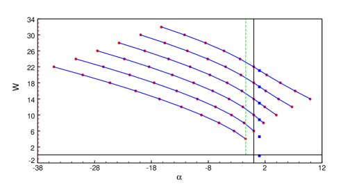
Figure 2: Eigenvalues $W_{n,0}$ obtained from the truncation condition (red circles) and by means of the variational method (blue squares)

Table 1: Lowest variational eigenvalues $W_{\nu,0}$ for $l=0$ and $\alpha=-\sqrt{2}$

$N$	$W_{0,0}$	$W_{1,0}$	$W_{2,0}$	$W_{3,0}$
$2$	$4.000000000$	$10.49997602$
$3$	$4.000000000$	$7.751061995$	$19.88102859$
$4$	$4.000000000$	$7.694010921$	$11.97562584$	$33.92039998$
$5$	$4.000000000$	$7.693979367$	$11.51212379$	$17.05520450$
$6$	$4.000000000$	$7.693978905$	$11.50604696$	$15.46896992$
$7$	$4.000000000$	$7.693978892$	$11.50604243$	$15.37652840$
$8$	$4.000000000$	$7.693978891$	$11.50604238$	$15.37592761$
$9$	$4.000000000$	$7.693978891$	$11.50604238$	$15.37592718$
$10$	$4.000000000$	$7.693978891$	$11.50604238$	$15.37592718$

Table 2: Lowest variational eigenvalues $W_{\nu,0}$ for $l=0$ and $\alpha=\sqrt{2}$

$N$	$W_{0,0}$	$W_{1,0}$	$W_{2,0}$	$W_{3,0}$
$2$	$-1.180391283$	$4.000000000$
$3$	$-1.401182256$	$4.000000000$	$9.284143096$
$4$	$-1.449885589$	$4.000000000$	$8.345259771$	$17.66452696$
$5$	$-1.458156835$	$4.000000000$	$8.344361267$	$12.69095166$
$6$	$-1.459389344$	$4.000000000$	$8.344349784$	$12.53313315$
$7$	$-1.459560848$	$4.000000000$	$8.344349442$	$12.53290257$
$8$	$-1.459583736$	$4.000000000$	$8.344349427$	$12.53290132$
$9$	$-1.459586704$	$4.000000000$	$8.344349427$	$12.53290130$
$10$	$-1.459587081$	$4.000000000$	$8.344349427$	$12.53290130$
$11$	$-1.459587128$	$4.000000000$	$8.344349427$	$12.53290130$
$12$	$-1.459587134$	$4.000000000$	$8.344349427$	$12.53290130$
$13$	$-1.459587134$	$4.000000000$	$8.344349427$	$12.53290130$

References

- [1] K. Bakke, Int. J. Mod. Phys. A 29, 1450117 (2014).
- [2] F. M. Fernández, Dimensionless equations in non-relativistic quantum mechanics, arXiv:2005.05377 [quant-ph].
- [3] L. D. Landau and E. M. Lifshitz, Quantum Mechanics. Non-relativistic Theory (Pergamon, New York, 1958).
- [4] C. Cohen-Tannoudji, B. Diu, and F. Laloë, Quantum Mechanics (John Wiley & Sons, New York, 1977).
- [5] A. DeSousa Dutra, Phys. Lett. A 131, 319 (1988).
- [6] S. Bera, B. Chakrabarti, and T. K. Das, Phys. Lett. A 381, 1356 (2017).
- [7] M. S. Child, S-H. Dong, and X-G. Wang, J. Phys. A 33, 5653 (2000).
- [8] F. L. Pilar, Elementary Quantum Chemistry (McGraw-Hill, New York, 1968).
- [9] F. M. Fernández, Q. Ma, and R. H. Tipping, Phys. Rev. A 39, 1605 (1989).
- [10] K. Bakke, Int. J. Mod. Phys. A 25, 2075003 (2020).
- [11] A. Verçin, Phys. Lett. B 260, 120 (1991).
- [12] J. Myrheim, E. Halvorsen, and A. Verçin, Phys. Lett. B 278, 171 (1992).