The anomalous atmospheric structure of the strongly magnetic Ap star HD 166473

Abstract

High resolution spectropolarimetric observations of the strongly magnetic, super-slowly rotating rapidly oscillating Ap star HD 166473 are used to investigate the implications of the presence of a variable strong magnetic field on the vertical and surface horizontal distribution of various chemical elements. The analysis of the calculated LSD Stokes $I$ and $V$ profiles confirms the previously reported detection of non-uniform horizontal surface distribution of several chemical elements. To test the vertical abundance stratification of iron peak and rare earth elements, magnetic field measurements were carried out using spectral lines of these elements belonging to neutral and ionised stages. We find clear indication of the existence of a relation between the magnetic field strength and its orientation and vertical element stratification: magnetic field values obtained for elements in different stages close to the magnetic equator are rather similar whereas the dispersion in field strengths is remarkably large in the regions close to magnetic field poles. At the phases of negative and positive extrema the mean longitudinal field strength determined from the analysis of the REE lines is usually stronger than when using Fe and Cr. The strongest mean longitudinal magnetic field, up to $-$4160$\pm$226 G, is detected using the La ii line list at the negative extremum, followed by the measurements using the Pr iii lines with $\langle B_{z}\rangle$=$-$3740$\pm$343 G and the Ce ii lines with $\langle B_{z}\rangle$=$-$3372$\pm$247 G. The strongest mean longitudinal magnetic field of positive polarity, up to 3584$\pm$354 G is detected using the Pr iii lines, followed by the measurement $\langle B_{z}\rangle$=2517$\pm$249 G using the Ce ii lines.

1 Introduction

The discovery of the presence of resolved magnetically split lines in the slowly rotating, cool Ap star HD 166473 (CoD $-37$ 12303) was reported by Mathys et al. (1997). The values of the mean magnetic field modulus that they measured range from 6.4 to 8.6 kG. Mathys & Hubrig (1997) had previously obtained for HD 166473 three measurements of the mean longitudinal field, all of the order of $-2$ kG. Kurtz & Martinez (1987) discovered rapid oscillations in this star, whose fundamental parameters, $T_{\rm eff}=7700$ K and $\log\,g=4.2$, were determined by Gelbmann et al. (2000). Kurtz & Martinez (1987) reported the existence of at least three pulsation modes with periods between 8.8 and 9.1 min and rather low photometric amplitudes (less than 0.5 mmag).

Most recently, Mathys, Khalack, & Landstreet (2020, hereafter MKL2020) presented the first accurate determination of the rotation period of HD 166473, $P_{\mathrm{rot}}=3836\pm 30$ d, from the analysis of 56 measurements of the mean magnetic field modulus $\langle B\rangle$ and 21 determinations of the mean longitudinal magnetic field $\langle B_{z}\rangle$. The latter were based on high- and medium-resolution spectra acquired between 1992 and 2019 at various observatories and with various instrumental configurations, among them high-resolution ESPaDOnS and HARPSpol polarimetric spectra. The value of the period derived by MKL2020, which is primarily based on the analysis of very precise measurements of the mean magnetic field modulus spanning 2.6 rotation cycles, is strongly constrained by the availability between phases 0.05 and 0.25 of several observations obtained at similar phases during three different rotation cycles. In particular, the alternative value of the period, $P_{\mathrm{rot}}=3893$ d, that was proposed by Bychkov, Bychkova, & Madej (2020) is extrapolated since it is based on observations spanning slightly less than a rotation cycle. It is definitely too long, as the $\langle B\rangle$ variation curve obtained using it to plot the whole data set of MKL2020 shows systematic phase shifts from one cycle to the next.

HD 166473, whose mean magnetic field modulus varies between 6 and 11 kG, possesses the third strongest field among roAp stars: stronger fields have been previously detected only in HD 154708 (24.5 kG, Hubrig et al., 2005; Kurtz et al., 2006) and HD 92499 (8.2 kG, Elkin et al., 2010). The variation curves of $\langle B\rangle$ and $\langle B_{z}\rangle$ are well approximated by cosine waves. The $\langle B_{z}\rangle$ variation curve shows sign reversals, implying that both magnetic poles of the star come alternately into sight over the rotation cycle. However, the phases of the extrema of the two field moments are shifted with respect to each other by a small but formally significant amount. The difference in the values of $\langle B\rangle$ between the phases of the extrema of $\langle B_{z}\rangle$, and the large ratio between the values of the $\langle B\rangle$ extrema further indicates that the structure of the magnetic field of HD 166473 departs significantly from a centred dipole (MKL2020).

Evidence that singly and doubly ionised Pr and Nd lie in a thin layer high in the atmosphere of HD 166473 was presented for the first time by Gelbmann et al. (2000). Furthermore, Cowley et al. (2001) identified a strong core-wing anomaly in the H Balmer lines: that is, the broad wings of these lines end abruptly in narrow cores. This indicates an extremely abnormal temperature-depth structure of the atmosphere. Kurtz, Elkin & Mathys (2003) took advantage of this anomalous atmospheric structure to study the vertical resolution of the pulsation modes into standing waves in the atmosphere and overlying running waves in the upper atmosphere. They also showed that the core of the H$\alpha$ line is formed deeper than the Pr and Nd lines, that stronger Pr and Nd lines form higher up in the atmosphere than the weaker ones, and that Fe lines form below the level of H$\alpha$ core formation, probably near radial pulsation nodes for all three modes.

A few years ago, Hubrig et al. (2018) analysed high-quality spectropolarimetric material obtained with HARPSpol for Przybylski’s star (HD 101065), a very slowly rotating star with a probable period of 188 yr and $\langle B_{z}\rangle$ of several hundred Gauss. They used longitudinal magnetic field measurements to discuss the anomalous structure of the atmosphere, in particular the inhomogeneous vertical distribution of several chemical elements. However, because Przybylski’s star rotates much more slowly than HD 166473, the structure of its magnetic field remains undefined. The availability of the high-resolution ESPaDOnS and HARPSpol spectropolarimetric observations of HD 166473 used in the recent magnetic field study of MKL2020 makes it possible now to investigate for this star the relation between the vertical and horizontal distribution of various chemical elements and the magnetic field structure.

Although the simple axisymmetric model of the magnetic field of HD 166473 that was obtained by MKL2020 is not meant to be physically realistic, its availability makes this star an excellent target for a detailed study of the non-uniform vertical and horizontal distributions of different chemical elements and their relation to the magnetic field strength and orientation. Such a study based on magnetic field measurements using line lists constructed for various elements in the neutral state and in various ionisation stages has the potential to provide an important test of the competing atomic segregation processes whose combination is generally believed to lead to the inhomogeneous and stratified atmospheres of the magnetic Ap stars.

In the following two sections we describe the observational material and the method of analysis. The obtained results and their discussion are presented in Sections 4 and 5.

2 Observations and data reduction

Table 1: Logbook of the observations. The columns give the telescope and instrument configuration, the heliocentric Julian date (HJD), rotation phase $\varphi$, and the exposure time. The rotation phase is calculated using the rotation period, $P_{\mathrm{rot}}=3836$ d, and the phase origin, HJD${}_{0}=2448660.0$, adopted by MKL2020.

Configuration	HJD	$\varphi$	Exp. time
	2 450 000+		[s]
ESO 3.6 m + HARPS	6148.655	0.952	1800
CFHT + ESPaDOnS	6531.773	0.052	2060
	6547.732	0.056	2060
	6813.014	0.125	2040
	7239.836	0.237	1014
	7287.712	0.249	2028
	8642.993	0.602	2096

The observations used in this study were already described in detail by MKL2020. The spectropolarimetric material analysed by these authors included seven high-resolution spectropolarimetric observations obtained at different epochs: six were acquired with the ESPaDOnS spectropolarimeter fed by the Canada-France-Hawaii Telescope (CFHT), and one with the High Accuracy Radial velocity Planet Searcher (HARPS) in spectropolarimetric mode fed by the ESO 3.6-m telescope. The logbook of the observations is presented in Table 1. The rotation phase is calculated using the rotation period, $P_{\mathrm{rot}}=3836$ d, and the phase origin, HJD${}_{0}=2448660.0$, adopted by MKL2020. The obtained spectra sample rather well the rotation cycle from phase 0.95 to phase 0.60, allowing us to analyse magnetic field measurements covering about two thirds of the rotation cycle including rotation phases close to the negative and positive extrema.

3 Magnetic field measurements

Similar to the previous study of Przybylski’s star (Hubrig et al., 2018), to measure the mean longitudinal magnetic field and to increase the signal-to-noise ratio (S/N), we employ the least squares deconvolution technique (LSD; Donati et al., 1997). This technique assumes that the lines used in the analysis have an identical shape and the resulting profile is scaled according to the line strength and sensitivity to the magnetic field. Using the Vienna Atomic Line Database (VALD; e.g., Kupka et al., 2011; Ryabchikova et al., 2015), we created 16 line masks for nine elements including the iron-peak elements Cr and Fe and seven rare-earth elements (REE), all based on the stellar parameters of HD 166473, $T_{\rm eff}=7700$ K and $\log\,g=4.2$ (Gelbmann et al., 2000). The line masks for Cr and Fe include lines belonging to the neutral atoms and the first ions. Line lists for first and second ions were created for Ce, Pr, Nd, Eu, and Er, whereas for La the identified lines of the second ion are too blended or weak and the only known Sm iii lines are at wavelengths shorter than 3850 Å. Those lines of the aforementioned ions that are located in spectral regions contaminated by telluric lines are not included in the line lists.

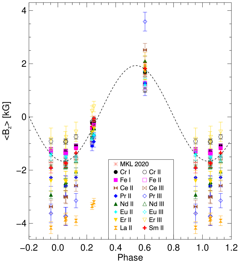
Figure 1: Mean longitudinal magnetic field $\langle B_{z}\rangle$ values calculated for various line masks at the phases listed in Table 1. Additionally, the $\langle B_{z}\rangle$ values from MKL2020 measured using exclusively Fe i lines (MKL 2020) are presented by asterisks and their best fit solution for the magnetic phase curve by the dashed line.

The mean longitudinal magnetic field is determined by computing the first-order moment of the LSD Stokes $V$ profile according to Mathys (1989):

$$\left<B_{\mathrm{z}}\right>=-2.14\times 10^{11}\frac{\int\upsilon V(\upsilon){\mathrm{d}}\upsilon}{\lambda_{0}g_{0}c\int[I_{c}-I(\upsilon)]{\mathrm{d}}\upsilon},$$ (1)

where $\upsilon$ is the velocity shift from the line centre, in km s^-1, and $\lambda_{0}$ and $g_{0}$ are the average values of, respectively, the wavelengths (in nm) and the effective Landé factors of all the lines used to compute the LSD profile.

The results of the LSD magnetic field measurements using 16 different line masks are presented in Table  2 along with the number of lines in each mask and the average Landé factors $g_{0}$. In most cases the false alarm probability (FAP) for the field detections is less than $10^{-6}$. According to Donati, Semel, & Rees (1992), a Zeeman profile with FAP $\leq 10^{-5}$ is considered as a definite detection, $10^{-5}<$ FAP $\leq 10^{-3}$ as a marginal detection, and FAP $>10^{-3}$ as a non-detection. In general, all the marginal or non-detections found for a few elements refer to the phases where the field polarity is turning from negative to positive. These are the measurements for Er ii and Eu iii at $\varphi=0.237$, for which we obtain only marginal detections with, respectively, $\mathrm{FAP}=2.4\times 10^{-5}$ and $\mathrm{FAP}=1.5\times 10^{-5}$. For Ce ii, Pr ii, and Sm ii at $\varphi=0.237$ and at $\varphi=0.249$, the FAPs are $>10^{-3}$. Er iii is a special case: only the last detection at $\varphi=0.602$ is a definite one while at $\varphi=0.237$ we get a non-detection. All the other Er iii phases give only marginal detections with FAPs just below $10^{-3}$. This is due to the very small number of clean unblended Er iii lines identified in the polarimetric spectra.

Table 2: Longitudinal magnetic field strength measurements using the LSD technique for 16 different line masks. In Column 2 we present the number of lines ($N$) in the individual line mask and the average Landé factor. For each line list, the seven rows in the Column 3 correspond to the epochs listed in Table 1.

	$N$	$\langle B_{z}\rangle$			$N$	$\langle B_{z}\rangle$
	$g_{0}$	[G]			$g_{0}$	[G]
Cr i	18	$-$1269$\pm$	104	Cr ii	19	$-$913$\pm$	102
	1.27	$-$1304$\pm$	95		1.25	$-$931$\pm$	96
		$-$1329$\pm$	111			$-$925$\pm$	101
		$-$1083$\pm$	75			$-$745$\pm$	88
		$-$230$\pm$	49			$-$176$\pm$	49
		$-$181$\pm$	56			$-$70$\pm$	44
		1684$\pm$	146			1009$\pm$	84
Fe i	120	$-$1282$\pm$	53	Fe ii	24	$-$1213$\pm$	77
	1.23	$-$1362$\pm$	66		1.20	$-$1299$\pm$	92
		$-$1370$\pm$	64			$-$1327$\pm$	96
		$-$1173$\pm$	50			$-$1100$\pm$	81
		$-$417$\pm$	31			$-$414$\pm$	41
		$-$300$\pm$	27			$-$225$\pm$	36
		1256$\pm$	75			1193$\pm$	157
Ce ii	14	$-$3372$\pm$	247	Ce iii	7	$-$1669$\pm$	170
	1.01	$-$2995$\pm$	236		1.26	$-$1720$\pm$	193
		$-$3016$\pm$	246			$-$1697$\pm$	195
		$-$2583$\pm$	211			$-$1560$\pm$	166
		$-$764$\pm$	164			$-$931$\pm$	101
		$-$168$\pm$	117			$-$750$\pm$	95
		2517$\pm$	249			1235$\pm$	267
Pr ii	7	$-$2277$\pm$	331	Pr iii	5	$-$3626$\pm$	352
	1.03	$-$2603$\pm$	397		0.97	$-$3732$\pm$	334
		$-$2591$\pm$	366			$-$3740$\pm$	343
		$-$2272$\pm$	356			$-$3145$\pm$	270
		$-$1091$\pm$	179			$-$1036$\pm$	94
		$-$928$\pm$	205			$-$696$\pm$	103
		1270$\pm$	468			3584$\pm$	354
Nd ii	20	$-$2925$\pm$	148	Nd iii	8	$-$1853$\pm$	59
	1.07	$-$2491$\pm$	168		1.36	$-$1890$\pm$	60
		$-$2451$\pm$	152			$-$1856$\pm$	59
		$-$2050$\pm$	137			$-$1658$\pm$	45
		$-$737$\pm$	102			$-$588$\pm$	34
		$-$412$\pm$	87			$-$417$\pm$	32
		2108$\pm$	196			1702$\pm$	105
Eu ii	7	$-$1399$\pm$	67	Eu iii	4	$-$1449$\pm$	193
	1.62	$-$1568$\pm$	65		1.15	$-$1676$\pm$	184
		$-$1531$\pm$	58			$-$1662$\pm$	206
		$-$1467$\pm$	50			$-$1515$\pm$	170
		$-$827$\pm$	32			$-$778$\pm$	99
		$-$684$\pm$	26			$-$687$\pm$	82
		1213$\pm$	74			1449$\pm$	256
Er ii	10	$-$2406$\pm$	397	Er iii	3	$-$834$\pm$	418
	1.11	$-$2408$\pm$	372		1.31	$-$954$\pm$	405
		$-$2433$\pm$	388			$-$760$\pm$	417
		$-$2088$\pm$	319			$-$560$\pm$	366
		$-$587$\pm$	91			218$\pm$	197
		$-$434$\pm$	105			391$\pm$	198
		1710$\pm$	318			1855$\pm$	446
La ii	15	$-$4160$\pm$	226	Sm ii	12	$-$1914$\pm$	192
	1.09	$-$3860$\pm$	215		1.14	$-$1715$\pm$	167
		$-$3816$\pm$	210			$-$1736$\pm$	155
		$-$3902$\pm$	183			$-$1354$\pm$	146
		$-$3346$\pm$	133			$-$350$\pm$	112
		$-$3207$\pm$	148			$-$66$\pm$	96
		1913$\pm$	506			1817$\pm$	214

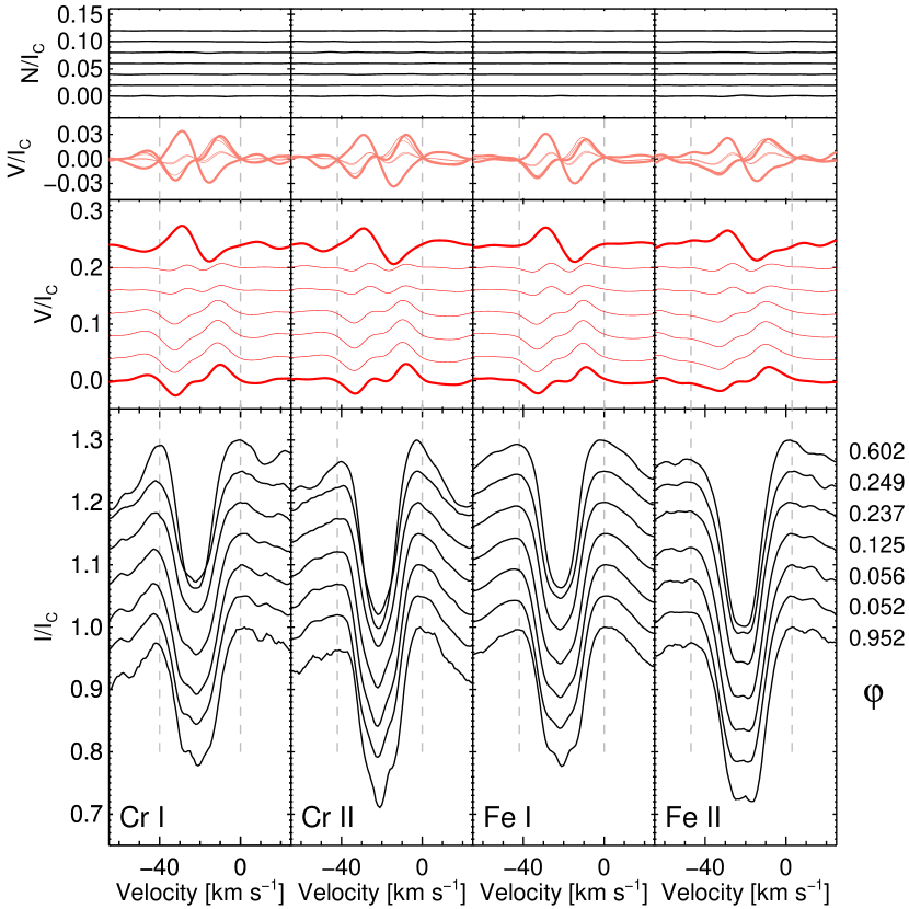
Figure 2: LSD Stokes $I$ (bottom), Stokes $V$ (middles), and diagnostic null ($N$) profiles (top) obtained for HD 166473 on seven nights. The LSD profiles were calculated using Cr i, Cr ii, Fe i, and Fe ii lines. The first Stokes $V$ observation obtained close to the negative field extremum and the last observation obtained close to the positive field extremum are highlighted by thicker red lines.

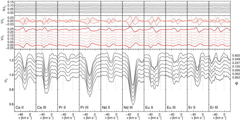
Figure 3: As Fig. 2, but for REEs with different ionisation stages: Ce ii, Ce iii, Pr ii, Pr iii, Nd ii, Nd iii, Eu ii, Eu iii, Er ii, and Er iii lines.

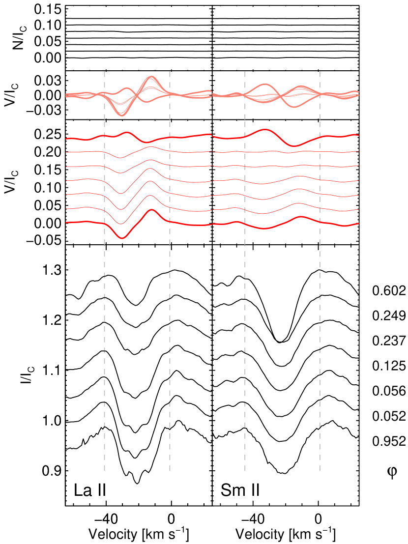
Figure 4: As Fig. 2, but using La ii and Sm ii line lists.

In Fig. 1 we display the mean longitudinal magnetic field values listed in Table  2, phased as in Table 1. In this figure we also show the field measurements of MKL2020, which are based exclusively on 20 Fe i lines. The dashed curve is the best sinusoidal least-squares fit solution for the phase curve defined by magnetic field measurements presented in MKL2020. For fitting parameters and more details we refer to MKL2020. We note that, in general, the absolute values of the longitudinal field that are determined using all REE line masks are significantly larger close to the phases of the two extrema than the absolute values that are obtained using lines belonging to the Fe and Cr line masks. The largest absolute values of the mean longitudinal magnetic field at the rotation phases corresponding to the negative extremum, up to $-$4160$\pm$226 G, are derived using the La ii line list, followed by the measurements using the Pr iii line list with $\langle B_{z}\rangle$=$-$3740$\pm$343 G and the Ce ii line list with $\langle B_{z}\rangle$=$-$3372$\pm$247 G. The largest positive value of the mean longitudinal magnetic field, up to 3584$\pm$354 G, is derived using the Pr iii line list, followed by the measurement using the Ce ii line list, with $\langle B_{z}\rangle$=2517$\pm$249 G.

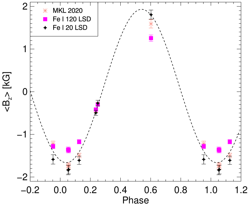
Figure 5: Comparison of the mean longitudinal magnetic field values obtained by MKL2020 by application of the moment technique with the LSD determinations based on the list of 20 Fe i lines of this reference and on the full list of 120 Fe i lines of this analysis. The fit as in Fig. 1.

The values of $\langle B_{z}\rangle$ that are derived from the analysis of the Fe i line list differ significantly from the values obtained by MKL2020, at least close to the phases of the extrema of the mean longitudinal magnetic field. At these phases, differences of the order of 350 G are found between the results of the two analyses, which represents $\sim$20–30% of the actual field values.

To gain insight into the origin of these discrepancies, we determined $\langle B_{z}\rangle$ by application of the LSD technique to the Fe i line list that MKL2020 analysed with the moment technique. As can be seen in Fig. 5, when applied to the same line list, both methods give measurements that are mostly consistent within their uncertainties. The small residual differences can almost certainly be attributed to the different assumptions underlying these methods. In particular, the interpretation of the measurements made with the moment technique rests on the weak-line approximation. This approximation is robust, in that even when its conditions are not strictly met, the resulting measurement errors tend to remain moderate. The weak-field approximation on which LSD relies is, however, more fragile, as departures from its validity tend to entail rapidly growing measurement errors. The magnetic field of HD 166473 is too strong for the weak-field approximation to be strictly valid. Thus, the small differences between the $\langle B_{z}\rangle$ values derived by application to the same line list of the moment technique, on the one hand, and of LSD, on the other, almost certainly just reflect the respective limitations of the approximations on which they are based.

By contrast, the discrepancies between the results of the LSD analysis of two sets of Fe i lines are very significant. They must be attributed to the different characteristics of these two line sets. The list used in the rest of the present study comprises 120 Fe i lines, while there are only 20 lines of this ion in the list of MKL2020. The two lists partly overlap, but that of MGL2020 is restricted to the wavelength interval 5400–6800 Å, while the full 120-line list spans the range 4400–6700 Å. As is well known, the continuum opacity in the visible changes significantly with wavelength, so that at the red end of the spectrum, one can observe lines that form in deeper photospheric layers than at the blue end. The resulting impact on the mean longitudinal magnetic field measurements is illustrated in Fig. 6. It shows the results of an experiment in which the LSD technique was applied to determine the mean longitudinal magnetic field of HD 166473 from two subsets, one blue and one red, of the line lists for Fe i and Fe ii. Among the ions studied here, Fe i and Fe ii have the longest line lists. The dividing wavelength between the two subsets was set at 5440 Å. There are 77 Fe i lines and 15 Fe ii lines blueward of this wavelength, and 43 Fe i lines and 9 Fe ii lines redward. One can see in Fig. 6 that the absolute values of $\langle B_{z}\rangle$ that are derived from the blue line lists are systematically smaller than those obtained from the red line lists. This trend is consistent with the expected behaviour of a dipole-like magnetic field, which should be more intense deeper in the stellar atmosphere than higher up, and with the fact that one can observe lines formed deeper in the photosphere at longer wavelengths.

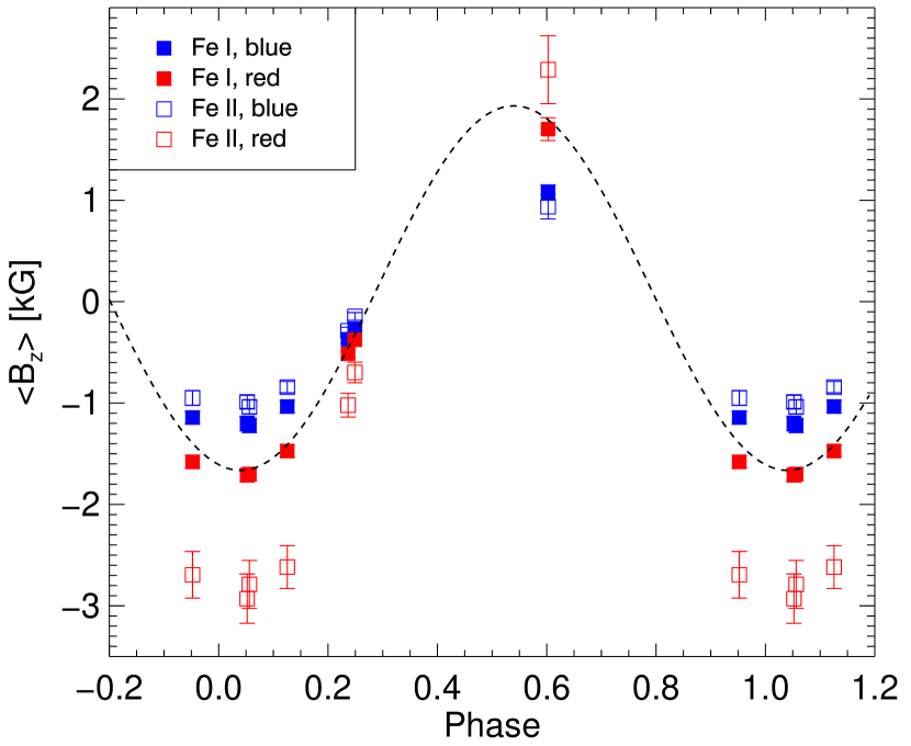
Figure 6: Comparison of the mean longitudinal magnetic field values obtained by application of the LSD technique to subsets of lines of Fe i (filled squares) and Fe ii (open squares) with wavelengths shorter (blue symbols) and longer (red symbols) than 5440 Å. The fit as in Fig. 1.

From consideration of the similarity of the $\langle B_{z}\rangle$ values obtained by application of the LSD and moment techniques to the set of (red) Fe i lines of MKL2020 restricted to the wavelength interval 5400–6800 Å, and the significant differences between the $\langle B_{z}\rangle$ values derived by applying the LSD technique to a blue and a red subset of Fe i lines, the discrepancies between the mean longitudinal magnetic field measurements of the present study and those of MKL2020 should be ascribed primarily to the different characteristics of the analysed line lists, especially with respect to their sampling of the wavelength range.

It should also be noted that the differences between the $\langle B_{z}\rangle$ values determined by using red and blue subsets of Fe ii lines are considerably larger than these differences for Fe i. This is probably related to the fact that the excitation energies of the lower levels of the observed Fe ii transitions span a much larger range ($\sim$10 eV) than those of the Fe i lines ($\sim$4.5 eV), so that the lines of the former are formed over a wider range of photospheric depths.

The LSD Stokes $I$, $V$, and diagnostic null ($N$) profiles for different ions of different elements are shown in Figs. 2–4. Null spectra are usually obtained by combining the different polarizations in such a way that polarization cancels out. In all studied cases they are essentially flat. At phases close to the negative extremum, the lines of certain elements show a partly resolved magnetically split structure in the Stokes $I$ LSD profiles; this structure appears different for different ions. The Fe i lines usually show a triplet structure while the Fe ii lines are doublets. A triplet structure is also apparent in the LSD Stokes $I$ line profiles of Ce ii, Pr ii, Pr iii, Nd iii, Eu ii, Er ii, Er iii, and La ii, whereas the profiles of Ce iii and Eu iii show a doublet structure. An interesting feature of the Eu iii LSD magnetically resolved doublet profiles is the stronger intensity of the blue components.

Because they often arise from transitions between atomic levels of high angular momentum $J$, the REE lines tend to have very broad anomalous Zeeman patterns. However, their effective Landé factors are in average smaller and span a narrower range of values than those of the lines of Fe and Cr. Statistically, the studied REE transitions display all the types of anomalous Zeeman patterns (see Fig. 1 of Mathys, 1989), with no particular preference overall. However, on an individual basis, the short line lists of certain ions may show a predominant occurrence of a certain pattern type. For instance, 6 of the 8 lines of Nd iii have a Zeeman pattern of Type 2, whereas this type is not represented among the 6 Eu ii lines, and 5 of the 7 lines of Pr ii have a Type 3 pattern (for more details, see Mathys, 1989). Furthermore, among the lines of the same type of a given ion, some show a wide spread of the individual components within each of the $\sigma_{-}$, $\pi$ and $\sigma_{+}$ sets of components, while for others, these sets are compact. Among the 112 REE lines that have been analysed, only 4 have a normal triplet pattern.

The observed LSD line profiles shown in Figs. 3 and 4 reflect the diversity of the Zeeman patterns and strengths of the individual lines from which they are computed. This is a complex combination that, in general, does not lend itself to simple intuitive interpretation. This complexity is further compounded by the effect of the hyperfine structure that affects several of the REE at various degrees. This effect may in particular be responsible for departures from symmetry of the Stokes $I$ profiles of some spectral lines, which form in a regime of Paschen-Back effect rather than Zeeman effect (Landolfi et al., 2001; Hubrig et al., 2002; Khalack & Landstreet, 2012).

4 Link between abnormal atmospheric composition and magnetic field strength and orientation

The calculated LSD profiles and the analysis of longitudinal magnetic field measurements over the rotation cycle indicate an extremely abnormal chemical composition of the atmosphere of HD 166473. In the following, we discuss in more detail the inhomogeneous horizontal and vertical element distribution at different rotation phases in relation with the different magnetic field strength and orientation.

4.1 Non-uniform horizontal element distribution

Mathys (2017) noted that the equivalent widths of the Fe i lines in HD 166473 are definitely variable. These line intensity variations were further characterised by MKL2020, who also reported and studied line-intensity variations for Nd iii. In both cases, they attributed those variations to non-uniform horizontal surface distribution of the chemical elements. Magnetic Ap stars are known to frequently display horizontal abundance inhomogeneities across their surfaces. Some elements, such as REE, are usually observed to concentrate close to the magnetic poles, whereas other elements prefer the regions close to the magnetic equator. Accordingly, the spectral lines of elements that have different distributions across the stellar surface sample the magnetic field topology in different manners (e.g., Kochukhov et al., 2004).

In Fig. 7, we present a number of Stokes $I$ profiles of individual lines belonging to different elements and the corresponding Stokes $V$ profiles, which show a complex structure. As illustrated in Figs. 2 and 3, a similarly complex structure with central features is also observed at the rotational phases close to the negative field extremum in the LSD Stokes $V$ profiles obtained for the Cr i, Cr ii, Fe i, Fe ii, Ce iii, Nd iii, Eu ii, and Eu iii line lists.

Figures 5 and 6 of MKL2020 illustrate how the presence of magnetic fields of opposite polarities and different strengths in the line-forming regions on different parts of the visible stellar hemisphere can produce structured Stokes V profiles. Following these authors, we attribute the complex structure of the Stokes $V$ profiles (both individual and LSD) of various ions to the presence of magnetic fields of mixed polarities over the hemisphere of HD 166473 that is facing us around the phase of the negative extremum of $\langle B_{z}\rangle$. By contrast, close to phase 0.6, the Stokes $V$ line profiles are mostly S-shaped. Hence we expect the polarity of the magnetic field to be predominantly positive over most of the half of the stellar surface that is visible around the phase of the positive extremum of $\langle B_{z}\rangle$.

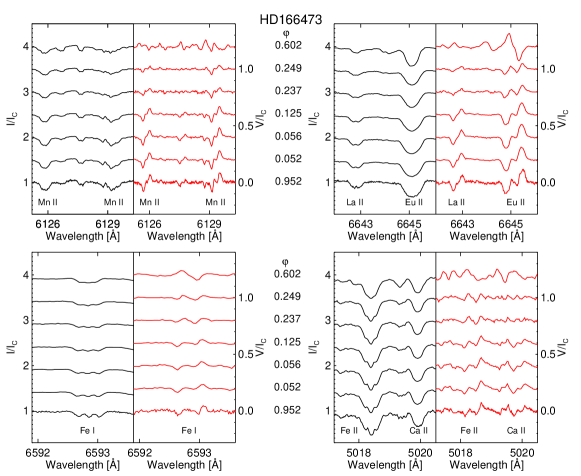
Figure 7: Variability of the Stokes $I$ (left) and Stokes $V$ (right) line profiles belonging to a few elements in different ionisation stages over the rotational cycle. The top left panel shows two Mn ii lines, the top right panel La ii and Eu ii lines, bottom left panel Fe i line, and bottom right panel Fe ii and Ca ii lines.

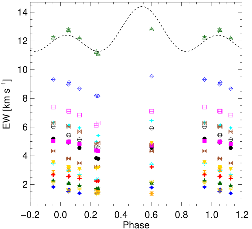
Figure 8: The equivalent widths (EWs) measured from LSD $I$ profiles of the different elements with different ionisation stages against the phases from Table 1. The symbols are as in Fig. 1. The error bars are usually of the symbol size as indicated for the measurements obtained using Nd iii lines. The dashed line is a cosine wave and its first harmonic fit obtained for Nd iii $\lambda 6145$ Å EWs by MKL2020 based on 56 data points.

In Fig. 8 we present the equivalent widths (EWs) measured from the LSD $I$ profiles obtained for different line masks, phased as in Table 1. Figures 7 and 8 of MKL2020 showed the EW variability of the Nd iii $\lambda 6145$ Å and Fe ii/i $\lambda 6147.7$ Å lines over the rotation cycle. Two maxima and two minima were detected in the variation curves, with the maxima occurring close to the phases of extrema of the magnetic field moments $\langle B_{z}\rangle$ and $\langle B\rangle$. Thus, both lines become stronger in the vicinity of magnetic poles. The primary maximum of the EW of the Nd iii line occurs close to the positive extremum of $\langle B_{z}\rangle$, while that of the Fe line coincides with the negative $\langle B_{z}\rangle$ extremum. Our measurements of the EW of the LSD profiles for the line lists of the ions considered in this study, which are shown in Fig. 8, suggest that the horizontal distribution of all of them is, to some extent, non-uniform. However, the phase sampling of our spectra is too sparse and uneven to constrain unambiguously the distribution of each element. While some are likely concentrated around the magnetic poles, similarly to Fe and Nd, we cannot definitely rule out different abundance patterns for some others. The fit shown in Fig. 8 is based on 56 data points of MKL2020.

4.2 Non-uniform vertical element distribution

In their abundance analysis of HD 166473, Gelbmann et al. (2000) concluded that, on average, the REEs are overabundant by $+$2.8 dex. The derived abundances of the second ions exceed the abundance values obtained from the lines of the first ions by $+$1.2 dex for Pr, $+$1.5 dex for Nd, and $+$0.7 dex for Er. At that time, the REE anomaly had only been discovered in $\gamma$ Equ (Ryabchikova et al., 1997) and it was found later in other roAp stars (e.g., Ryabchikova et al., 2001). The REE anomaly that is observed in HD 166473 cannot be explained by a wrong absolute scale of the oscillator strengths; hyperfine structure and isotopic shifts cannot be responsible either for the differences between the abundances of the second and third REE ions (e.g., Gelbmann et al., 2000; Ryabchikova et al., 2001). Instead, the anomaly is usually assigned to the vertical stratification of the abundances of the REEs. According to Michaud, Alecian, & Richer (2015), in the hydrodynamically stable atmospheres of Ap and Bp stars, atomic diffusion can be responsible for horizontal and vertical stratification of abundances. Magnetic fields observed in these stars could further stabilize the upper atmospheric layers and significantly amplify atomic diffusion, causing the existence of overabundance patches in certain areas of the stellar atmosphere and vertical abundance stratification (Stift & Alecian, 2016; Alecian & Stift, 2017, 2019). In some cases, the light and iron-peak elements are concentrated in the deeper atmospheric layers, whereas the REEs accumulate in the upper atmospheric layers (e.g., Bohlender et al., 2000; Ryabchikova et al., 2004).

As HD 166473 has been observed polarimetrically at seven different rotation phases sampling different regions of the stellar surface with different magnetic field strength and orientation, it appears to be an excellent target to investigate the implications of the magnetic field strength and orientation on the vertical abundance stratification of various elements. In particular, the available observations sample the parts of the stellar surface around the negative and positive magnetic poles and around the magnetic equator. This permits a study of the abundance stratification in regions with very different inclinations of the magnetic field lines.

To test the abundance stratification of various elements in the atmospheres in the strongly magnetic star HD 166473, we analysed the differences of magnetic field measurements using line masks constructed for two different ions of various elements. The results of this experiment are shown in Fig. 9. For normal A-type star atmospheres, we expect the lines of elements in the higher ionisation stage to be formed lower in the atmosphere than those of elements in the lower ionisation stage. Under the assumption that this is also the case in HD 166473 and that the structure of its magnetic field is predominantly dipolar, we would expect to measure a stronger magnetic field in the lines belonging to the elements in the higher ionisation stage. We do not actually know the magnetic geometry of this star, as the model adopted by MKL2020 was not meant to be physically realistic, but the arguments presented by these authors suggest that it is reasonable to use a dipole-like depth dependence of the photospheric magnetic field strength and orientation for the present analysis.

The absolute values of the mean longitudinal magnetic field determined from consideration of the lines of neutral Cr are systematically larger than those derived from analysis of the lines of the first ion. The marginal $\langle B_{z}\rangle$ value differences between Fe i and Fe ii that appear in Fig. 9 may at first sight seem inconsistent with the behaviour illustrated in Fig. 6 for the measurements performed using separately the blue or the red subsets of lines. That the discrepancies between the mean longitudinal magnetic field values derived from the two ions with each of these subsets, which are of opposite sign, cancel out when the whole line list for each ion is analysed at once, must be considered as coincidental and partly due to the different sizes of the various line lists. Since Gelbmann et al. (2000) reported a slight overabundance of Cr and an essentially solar abundance of Fe, with no significant hint of abundance stratification of these elements, the ion-to-ion $\langle B_{z}\rangle$ differences for them must primarily reflect the distribution of the formation depths of the diagnostic lines, as resulting from the excitation potential of their lower levels and from their strength.

Longitudinal field measurements using lists of lines of the first and second ions of REE indicate that the various elements have very different stratifications. While measurements using the line lists belonging to the Ce and Nd first ions show a significantly stronger longitudinal field close to the phases of the magnetic extrema, Pr shows the opposite behaviour at the same phases, with much stronger $\langle B_{z}\rangle$ values derived from the second ion line list. Furthermore, the difference between the field values measured using the lists of the first and second ions of Pr is surprisingly large, reaching about 1.3 kG close to the negative extremum of the longitudinal field and 2.3 kG near its positive extremum. Almost identical $\langle B_{z}\rangle$ values within the measurement uncertainties were obtained for the first and second ions of Eu. Measurements using the line lists for the first and second Er ions mostly follow the trend detected for Ce and Nd, except in the vicinity of the positive magnetic pole, where the $\langle B_{z}\rangle$ values are obtained from the analysis of the lines of either ion do not significantly differ from each other.

The LSD Stokes $I$ and Stokes $V$ profiles of the remaining lanthanide elements, La and Sm, are presented in Fig. 4. For these elements, the only blend-free lines that could be identified in the spectra belong to the first ionisation stage. The magnetic field of the order of $-$4.2 kG measured in the vicinity of the negative magnetic pole using the line list for La ii lines is the strongest of all the values obtained in this analysis, followed by $\langle B_{z}\rangle=-3.7$ kG values determined from the analysis of Pr iii lines.

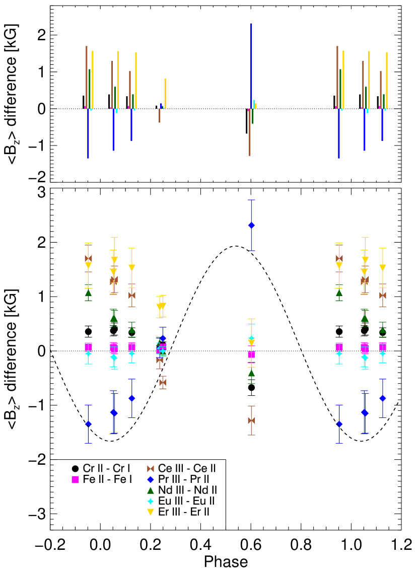
Figure 9: Bottom panel: The differences in the longitudinal magnetic field measurements between the first ionization stage and the neutral stage for Cr and Fe and the second and the first ionization stages for REEs. The dashed line is as in Fig. 1. Top panel: Histogram presentation of the differences. The colours of the bars are as the colours of the different symbols in the lower panel and the order of the bars for each phase follows the order given in the legend of the lower panel (from Cr to Er). For phases where we have two almost simultaneous measurements (around 0.05 and 0.24) the average value is used for clarity.

5 Discussion

We compared magnetic field measurements carried out using spectral lines belonging to two different ionisation stages of a number of elements. This analysis indicates that there exists a relation between the magnetic field strength and orientation, on the one hand, and vertical element stratification, on the other hand. Namely, at rotational phases such as $\varphi$=0.237 and 0.249, at which HD 166473 is observed magnetic equator-on, with the line of sight nearly making a right angle with the dipole axis, similar values of the longitudinal magnetic field values are obtained from consideration of the lines of the two ions of each element. By contrast, for observations obtained at epochs when the star is seen almost magnetic pole-on, very different $\langle B_{z}\rangle$ values are obtained from the analysis of lines corresponding to different ionisation stages, especially for the first and second ions of Ce, Pr, Nd and Er.

Table 3: Root-mean square mean longitudinal magnetic field values determined from $\langle B_{z}\rangle$ measurements at phases 0.952, 0.052, 0.056, and 0.602 from the spectral lines of the first and second ions of four REEs. The results obtained by application of the LSD and moment techniques are compared (top section). The differences between them, for a given ion (bottom section), and the differences between the first and second ion values, with each measurement technique (middle section), are given. The averages of the formal uncertainties of the $\langle B_{z}\rangle$ measurements for the line lists of each ion and for each measurement technique are also included. For the differences, $\Delta\langle B_{z}\rangle_{\rm rms}=\langle B_{z}\rangle_{{\rm rms},1}-\langle B_{z}\rangle_{{\rm rms},2}$, the values of $\sqrt{\sigma_{\rm av,1}^{2}(\langle B_{z}\rangle)+\sigma_{\rm av,2}^{2}(\langle B_{z}\rangle)}$ are used as estimates of the uncertainties ($\sigma(\Delta\langle B_{z}\rangle_{\rm rms})$).

	Moment technique		LSD technique
Ion	$\langle B_{z}\rangle_{\rm rms}$	$\sigma_{\rm av}(\langle B_{z}\rangle)$	$\langle B_{z}\rangle_{\rm rms}$	$\sigma_{\rm av}(\langle B_{z}\rangle)$
	(G)	(G)	(G)	(G)
Ce ii	1945	180	2990	245
Pr ii	1412	216	2252	391
Nd ii	2009	105	2511	166
Er ii	1989	250	2260	369
Ce iii	1648	208	1593	206
Pr iii	2332	278	3671	346
Nd iii	1943	113	1827	71
Er iii	1484	527	1186	422
	Moment technique		LSD technique
Ion	$\Delta\langle B_{z}\rangle_{\rm rms}$	$\sigma(\Delta\langle B_{z}\rangle_{\rm rms})$	$\Delta\langle B_{z}\rangle_{\rm rms}$	$\sigma(\Delta\langle B_{z}\rangle_{\rm rms})$
	(G)	(G)	(G)	(G)
Ce iii$-$Ce ii	$-$297	275	$-$1398	320
Pr iii$-$Pr ii	920	352	1419	522
Nd iii$-$Nd ii	$-$66	154	$-$684	180
Er iii$-$Er ii	$-$505	583	$-$1074	560
	First ion		Second ion
Element	$\Delta\langle B_{z}\rangle_{\rm rms}$	$\sigma(\Delta\langle B_{z}\rangle_{\rm rms})$	$\Delta\langle B_{z}\rangle_{\rm rms}$	$\sigma(\Delta\langle B_{z}\rangle_{\rm rms})$
	(G)	(G)	(G)	(G)
Ce	$-$1045	304	55	293
Pr	$-$840	446	$-$1339	444
Nd	$-$502	196	117	134
Er	$-$271	445	299	675

The element-to-element differences in the discrepancies between the mean longitudinal magnetic field values obtained from the analysis of sets of lines belonging to two ionisation stages suggest that different elements have different vertical stratifications. Especially intriguing are the measurements using Pr ii and Pr iii lines, which suggest that vertical stratification for this element differs strongly from that of other elements. This is reminiscent of the results obtained by Hubrig et al. (2018) in their study of the vertical stratification of Nd and Pr in the atmosphere of Przybylski’s star. Magnetic field measurements for this star were based on lists of Pr and Nd lines belonging to first and second ions. A stronger longitudinal magnetic field was detected using lines belonging to the first ion of Nd. Within the measurement uncertainties, almost identical $\langle B_{z}\rangle$ values were derived using Pr ii and Pr iii lines. This indicates that the vertical distribution of Pr in the photosphere of Przybylski’s star greatly differs from that of Nd.

Different magnetic field strengths determined using lines of elements in different ionisation stages can in principle be explained by introducing element abundance layers for different ions in the outer atmosphere at different geometrical depths. The formation of such layers can be related to the existence of a non-standard temperature gradient. Based on the work of Shulyak et al. (2009), it is possible that if the strong overabundance of REEs is present in the atmosphere of HD 166473, it can lead to the appearance of an inverse temperature gradient with a maximum temperature increase of up to several hundreds Kelvin in the upper layers compared to a homogeneous abundance model. Admittedly, any scenario to understand the observed differences in magnetic field strengths is much more complicated. Atomic diffusion amplified by a magnetic field is expected to cause vertical abundance stratification in a hydrodynamically stable atmosphere. This stratification affects the radiative transfer in the atmosphere, in which as a result, the temperature gradient and the flux redistribution become non-standard. This in turn influences the diffusion process, making it time-dependent or dynamical (see Alecian & Stift, 2019). Clearly, more advanced theoretical simulations of atomic diffusion involving REEs are necessary to understand the observed anomalous atmospheric structures in magnetic Ap stars.

As mentioned in Sect. 2, the magnetic model of MKL2020 is not meant to be physically realistic, and one should be cautious not to overinterpret its implications. That the actual field structure departs from a dipole is consistent with the view that a purely dipolar configuration is not stable (Braithwaite & Nordlund, 2006), and it is likely that, contrary to a simple dipole, the magnetic field of HD 166473 is not force-free. Accordingly, the anomalous atmospheric structure of HD 166473 can be additionally affected by the presence of electromagnetic Lorentz forces. The impact of electric currents on the equivalent widths of hydrogen lines was previously studied by Madej (1983), who also reported that electromagnetic forces can significantly modify the pressure and temperature stratification of the atmosphere, leading to noticeable changes of ionization degree of some elements.

In view of the difference between the values of the mean longitudinal magnetic field that are derived by application of the LSD technique to different lists of Fe i lines (see Sect. 3), one may wonder to which extent the different values of $\langle B_{z}\rangle$ that are obtained from the consideration of the lines of different REE ions are just an artefact of the analysis method. This concern is further strengthened by the great diversity of the Zeeman patterns of the REE diagnostic lines (see also Sect. 3). Indeed, a fundamental assumption underlying the LSD technique is that “most lines [$\ldots$] exhibit Zeeman signatures with more or less the same shape” (Donati et al., 1997). The limited validity of this assumption when lines with very different Zeeman patterns are analysed has an unknown impact on the derived values of the mean longitudinal magnetic field.

To assess in a more quantitative manner the potential implications of these technical limitations for the physical conclusions that we derived from our $\langle B_{z}\rangle$ measurements, we repeated these measurements applying the moment technique, using the line lists of the four REE elements for which the values of the mean longitudinal magnetic field show significant differences between the first and the second ion (Ce, Pr, Nd, and Er). We considered only the four phases closest to the magnetic extrema (0.952, 0.042, 0.056, and 0.602), at which the ion-to-ion $\langle B_{z}\rangle$ differences are largest. For each ion, we computed the rms longitudinal field $\langle B_{z}\rangle_{\rm rms}$ (Bohlender, Landstreet, & Thompson, 1993) for these four phases. As an estimate of the uncertainty affecting the $\langle B_{z}\rangle_{\rm rms}$ values, we adopted the arithmetic mean of the formal uncertainties of the four individual measurements from which they were computed, $\sigma_{\rm av}(\langle B_{z}\rangle)$. The results of this experiment appear in the top section of Table 3. In the middle section of this table, we give the $\langle B_{z}\rangle$ differences between the two ions of each element, with each measurement technique. Their “uncertainties”, $\sigma(\Delta\langle B_{z}\rangle_{\rm rms})$, are computed by application of the standard error propagation formula to the corresponding individual uncertainties of the rms longitudinal field values, $\sigma_{\rm av}(\langle B_{z}\rangle)$. Finally, in the bottom section of Table 3, we present for each ion the differences between the $\langle B_{z}\rangle_{\rm rms}$ values based on the field determinations through the moment technique and through the LSD technique. The “uncertainties” are computed in the same way as in the middle sector.

The differences $\Delta\langle B_{z}\rangle_{\rm rms}$ between the values of the rms longitudinal field obtained from the analysis of the first and second ions of each of the considered elements are systematically larger with the LSD technique than with the moment technique. Actually, with the latter, $\Delta\langle B_{z}\rangle_{\rm rms}$ is considerably larger than its estimated uncertainty $\sigma(\Delta\langle B_{z}\rangle_{\rm rms})$ only for Pr. For the other REEs, the moment technique does not indicate the ion-to-ion $\langle B_{z}\rangle$ differences that are apparent with the LSD technique. Furthermore, for several ions (e.g. Pr iii), the difference between the $\langle B_{z}\rangle_{\rm rms}$ values obtained with the two $\langle B_{z}\rangle$ measurement techniques is as large or larger than the difference between the $\langle B_{z}\rangle_{\rm rms}$ values determined from the analysis of the two ions, by application of either technique. This calls for caution in the interpretation of the ion-to-ion $\langle B_{z}\rangle$ differences.

The most clear-cut case is that of Pr, for which a stronger mean longitudinal magnetic field seems definitely obtained from consideration of the lines of the second ion than of the first ion, both through the moment technique and with LSD. The resulting inference about abundance stratification appears well founded. The cases of Ce, Nd, and Er are less conclusive given that the analysis based on the moment technique fails to fully confirm the differences between the $\langle B_{z}\rangle$ values derived from the consideration of the first and second ions of each element when using LSD. The occurrence of abundance stratification for these elements, as suggested by the LSD analysis, is plausible, but further evidence is required to establish it convincingly and characterise it better.

Figure 3 illustrates the LSD profiles for the lanthanide elements Ce, Pr, Nd, Eu, and Er in the first and second ionisation stages. Among the studied lanthanides, Pr iii and Nd iii show by far the strongest lines. These lines are also much stronger than those of these elements in the first ionisation stage. Stronger lines with higher opacities form higher in the atmosphere (Kurtz, Elkin & Mathys, 2003). According to Mashonkina, Ryabchikova & Ryabtsev (2005) and Mashonkina et al. (2009), the formation of the Pr and Nd lines can significantly deviate from the local thermo-dynamic equilibrium (LTE). Thus, the doubly ionised lines of these elements appear unusually strong due to the combined effects of vertical stratification and departures from LTE. As shown by Mashonkina, Ryabchikova & Ryabtsev (2005) and Mashonkina et al. (2009), the departures from LTE for the Pr and Nd lines of the first and the second ions are of the opposite sign, and they are significant if these elements are concentrated in the upper atmospheric layers. In these studies, the effect of the magnetic field was omitted from the statistical equilibrium calculations. More theoretical work is required to understand the impact of NLTE on the line formation of various elements in the presence of a strong magnetic field.

To study the influence of a magnetic field on the atomic diffusion of different chemical elements in the hydrodynamically stable atmosphere of the Ap and Bp stars, Stift & Alecian (2016) have developed theoretical models of the time-dependent atomic diffusion. Depending on the strength and orientation of the magnetic field lines, time-dependent atomic diffusion can lead to accumulation of iron peak elements in the upper atmospheric layers even for a relatively weak magnetic field, of the order of 1 kG. Stift & Alecian (2016) have noted that the accumulation of iron in the outer atmosphere can lead to a temperature increase, a temperature plateau, or even a temperature inversion. Exploring the case of a non-axisymmetric magnetic field geometry (Stift et al., 2013, like in HD 154708) Alecian & Stift (2017) have modelled the 3D distribution of 16 chemical elements for equilibrium solutions and revealed rings or quasi-rings of enhanced Fe and Cr abundance in the upper atmospheric layers.

Recently, Alecian & Stift (2019) have demonstrated that in order to properly approximate the observational profile of the vertical stratification of elemental abundances in Ap and Bp stars using theoretical models of the time-dependent atomic diffusion, one needs to introduce a certain mass loss rate. The observational profiles of vertical abundance stratification derived for different chemical elements in the atmospheres of Ap and Bp stars in the framework of project VeSElkA (Vertical Stratification of Element Abundances; Khalack & LeBlanc, 2015a, b) may help one to constrain the theoretical models of time-dependent atomic diffusion. Therefore a detailed analysis of the vertical stratification of elemental abundances in the magnetically controlled atmosphere of the very slowly rotating Ap star HD 166473 will contribute to verifying observationally the impact of stellar rotation and magnetism on the time dependent-atomic diffusion, improving our understanding of this process.

Data Availability

The ESPaDOnS data underlying this article are available in the CFHT Science Archive at https://www.cadc-ccda.hia-iha.nrc-cnrc.gc.ca/en/cfht/ and can be accessed with the object name. Similarly, the HARPS data are available in the ESO Science Archive Facility at http://archive.eso.org/cms.html.

References

- Alecian & Stift (2017) Alecian G., Stift M. J., 2017, MNRAS, 468, 1023
- Alecian & Stift (2019) Alecian G., Stift M. J., 2019, MNRAS, 482, 4519
- Bohlender, Landstreet, & Thompson (1993) Bohlender D. A., Landstreet J. D., Thompson I.-B., 1993, A&A, 269, 355
- Braithwaite & Nordlund (2006) Braithwaite J., Nordlund Å., 2006, A&A, 450, 1077
- Bychkov, Bychkova, & Madej (2020) Bychkov V. D., Bychkova L. V., Madej J., 2020, arXiv:2004.14099
- Bohlender et al. (2000) Cowley C. R., Ryabchikova T., Kupka F., Bord D. J., Mathys G., Bidelman W. P., 2000, MNRAS, 317, 299
- Cowley et al. (2001) Cowley C. R., Hubrig S., Ryabchikova T. A., Mathys G., Piskunov N., Mittermayer P., 2001, A&A, 367, 939
- Donati, Semel, & Rees (1992) Donati J.-F., Semel M., Rees D. E., 1992, A&A, 265, 669
- Donati et al. (1997) Donati J.-F., Semel M., Carter B. D., Rees D. E., Collier Cameron A., 1997, MNRAS, 291, 658
- Elkin et al. (2010) Elkin V. G., Kurtz D. W., Mathys G., Freyhammer L. M., 2010, MNRAS, 404, L104
- Gelbmann et al. (2000) Gelbmann M., Ryabchikova T., Weiss W. W., Piskunov N., Kupka F., Mathys, G., 2000, A&A, 356, 200
- Hubrig et al. (2002) Hubrig S., Cowley C. R., Bagnulo S., Mathys G., Ritter A., Wahlgren G. M., in Exotic Stars as Challenges to Evolution, eds. C. A. Tout & W. Van Hamme, ASP Conf. Ser. 279, 365
- Hubrig et al. (2005) Hubrig S., et al., 2005, A&A, 440, L37
- Hubrig et al. (2018) Hubrig S., Järvinen S. P., Madej J., Bychkov V. D., Ilyin I., Schöller M., Bychkova L. V., 2018, MNRAS, 477, 3791
- Khalack & Landstreet (2012) Khalack V., Landstreet J. D., 2012, MNRAS, 427, 569
- Khalack & LeBlanc (2015a) Khalack V., LeBlanc F., 2015a, AJ, 150, 2
- Khalack & LeBlanc (2015b) Khalack V., LeBlanc F., 2015b, Advances in Astronomy and Space Physics, 5, 3
- Kochukhov et al. (2004) Kochukhov O., Drake N. A., Piskunov N., de la Reza R., 2004, A&A, 424, 935
- Kupka et al. (2011) Kupka F., Dubernet M.-L., VAMDC Collaboration, 2011, Baltic Astronomy, 20, 503
- Kurtz & Martinez (1987) Kurtz D. W., Martinez P., 1987, MNRAS, 226, 187
- Kurtz, Elkin & Mathys (2003) Kurtz D. W., Elkin V. G., Mathys G., 2003, MNRAS, 343, L5
- Kurtz et al. (2006) Kurtz D. W., Elkin V. G., Cunha M. S., Mathys G., Hubrig S., Wolff B., Savanov I., 2006, MNRAS, 372, 286
- Landolfi et al. (2001) Landolfi M., Bagnulo S., Landi Degl’Innocenti M., Landi Degl’Innocenti E., 2001, in Magnetic Fields Across the Hertzsprung-Russell Diagram, eds. G. Mathys, S. K. Solanki & D. T. Wickramasinghe, ASP Conf. Ser., 248, 349
- Madej (1983) Madej J., 1983, Acta Astronomica, 33, 1
- Mashonkina, Ryabchikova & Ryabtsev (2005) Mashonkina L., Ryabchikova T., Ryabtsev A., 2005, A&A, 441, 309
- Mashonkina et al. (2009) Mashonkina L., Ryabchikova T., Ryabtsev A., Kildiyarova R., 2009, A&A, 495, 297
- Mathys (1989) Mathys G., 1989, Fundam. Cosm. Phys., 13, 143
- Mathys (2017) Mathys G., 2017, A&A, 601, A14
- Mathys & Hubrig (1997) Mathys G., Hubrig S., 1997, A&AS, 124, 475
- Mathys et al. (1997) Mathys G., Hubrig S., Landstreet J. D., Lanz T., Manfroid J., 1997, A&AS, 123, 353
- Mathys, Khalack, & Landstreet (2020) Mathys G., Khalack V., Landstreet J. D., 2020, A&A, 636, 6
- Michaud, Alecian, & Richer (2015) Michaud G., Alecian G., Richer J., 2015, in Atomic Diffusion in Stars, Springer International Publishing Switzerland, p. 131
- Ryabchikova et al. (2001) Ryabchikova T. A., Savanov I. S., Malanushenko V. P., Kudryavtsev D. O., 2001, Astronomy Reports, 45, 382
- Ryabchikova et al. (1997) Ryabchikova T. A., Adelman S. J., Weiss W. W., Kuschnig R., 1997, A&A, 322, 234
- Ryabchikova et al. (2004) Ryabchikova T., Nesvacil N., Weiss W. W., Kockukhov O., Stütz C., 2004, A&A, 423, 705
- Ryabchikova et al. (2015) Ryabchikova T., Piskunov N., Kurucz R. L., Stempels H. C., Heiter U., Pakhomov Y., Barklem P. S., 2015, Phys. Scr., 90, 054005
- Shulyak et al. (2009) Shulyak D., Ryabchikova T., Mashonkina L., Kochukhov O. 2009, A&A, 499, 879
- Smalley et al. (2015) Smalley B., et al., 2015, MNRAS, 452, 3334
- Stift & Alecian (2016) Stift M. J., Alecian, G., 2016, MNRAS, 457, 74
- Stift et al. (2013) Stift M. J., Hubrig S., Leone F., Mathys G., 2013, in Shibahashi H.,Lynas-Gray A. E., eds, ASP Conf. Ser. Vol. 479, Progress in Physics of the Sun and Stars: A New Era in Helio- and Asteroseismology. Astron. Soc. Pac., San Francisco, p. 125