URLLC with Massive MIMO:
Analysis and Design at Finite Blocklength

Abstract

The fast adoption of Massive MIMO for high-throughput communications was enabled by many research contributions mostly relying on infinite-blocklength information-theoretic bounds. This makes it hard to assess the suitability of Massive MIMO for ultra-reliable low-latency communications (URLLC) operating with short-blocklength codes. This paper provides a rigorous framework for the characterization and numerical evaluation (using the saddlepoint approximation) of the error probability achievable in the uplink and downlink of Massive MIMO at finite blocklength. The framework encompasses imperfect channel state information, pilot contamination, spatially correlated channels, and arbitrary linear spatial processing. In line with previous results based on infinite-blocklength bounds, we prove that, with minimum mean-square error (MMSE) processing and spatially correlated channels, the error probability at finite blocklength goes to zero as the number $M$ of antennas grows to infinity, even under pilot contamination. However, numerical results for a practical URLLC network setup involving a base station with $M=100$ antennas, show that a target error probability of $10^{-5}$ can be achieved with MMSE processing, uniformly over each cell, only if orthogonal pilot sequences are assigned to all the users in the network. Maximum ratio processing does not suffice.

I Introduction

Among the new use cases that will be supported by next generation wireless systems [2], some of the most challenging ones fall into the category of ultra-reliable low-latency communications (URLLC). For example, in URLLC for factory automation [3], small payloads on the order of $100$ bits must be delivered within hundreds of microseconds and with a reliability no smaller than $99.999\%$. To achieve such a high reliability, it is crucial to exploit diversity. Unfortunately, the stringent latency requirements prevent the exploitation of diversity in time. Furthermore, the use of frequency diversity is problematic, especially in the uplink where current standardization rules do not allow user equipments (UEs) to spread a packet over independently fading frequency resources. Thus, the spatial diversity offered by multiple antennas becomes critical to achieve the desired reliability. The latest instantiation of multiple antenna technologies is the so-called Massive MIMO (multiple-input multiple-output), which refers to a wireless network where base stations (BS), equipped with a very large number $M$ of antennas, serve a multitude of UEs via linear spatial signal processing [4]. Thanks to the intense research performed since its inception in 2010, the advantages of Massive MIMO in terms of spectral efficiency [5, 6], energy efficiency [7], and power control [8] are well understood, and its key ingredients have made it into the 5G standard [9]. However, all these results have mainly been established in the ergodic regime, where the propagation channel evolves according to a block-fading model, and each codeword spans an increasingly large number of independent fading realizations as the codeword length goes to infinity (infinite-blocklength regime). Since these assumptions are highly questionable in URLLC scenarios [10], it remains unclear whether the design guidelines that have been obtained so far for Massive MIMO (see [11, 12] for a detailed review on the topic) apply to URLLC deployments.

I-A Prior Art

Unlike the vast majority of literature on Massive MIMO, which focuses on the aforementioned ergodic regime, the authors in [13, 14] assume that the fading channel stays constant during the transmission of a codeword (the so-called quasi-static fading scenario) and use outage capacity [15] as asymptotic performance metric. Although the quasi-static fading scenario is relevant for URLLC, the infinite blocklength assumption may yield incorrect estimates of the error probability. The use of outage capacity in the context of URLLC is often justified by the results reported in [16], where it is proved that short channel codes operate close to the outage capacity for quasi-static fading channels. More specifically, the authors of [16] proved that the difference between the outage capacity and the maximum coding rate, achievable at finite blocklength over quasi-static fading channels, goes to zero much faster than the difference between the capacity and the maximum coding rate achievable over additive white Gaussian noise (AWGN) channels. The intuition is that the dominant sources of errors in quasi-static fading channels are deep-fade events, which cannot be alleviated through the use of channel codes, since channel coding provides protection only against additive noise.

The application of this result to Massive MIMO is problematic since, as $M$ grows, we start observing channel hardening and the underlying effective channel (after precoding/combining) becomes more similar to an AWGN channel. As a consequence, finite-blocklength effects become more pronounced, since additive noise turns into the dominating impairment. Another unsatisfactory feature of the outage-capacity framework is its inability to account for the channel state information (CSI) acquisition overhead, caused by the transmission of pilot sequences. Indeed, quasi-static fading channels can be learnt perfectly at the receiver in the asymptotic limit of large blocklength with no rate penalty: it is enough to let the number of pilot symbols grow sublinearly with the blocklength. The attempts made so far to include channel-estimation overhead in the outage setup [13, 14] are not convincing from a theoretical perspective. A theoretically satisfying framework must include the use of a mismatch receiver that treats the channel estimate, obtained using a fixed number of pilot symbols, as perfect. One difficulty is that a fundamental result commonly used in the ergodic case to bound the mutual information, by treating the channel estimation error as noise (see, e.g., [17, Lemma B.0.1]), does not apply to the outage case. This is because, in the outage setup, the fading channel stays constant over the entire codeword, and one is interested in computing an outage event over fading realizations. This means that both the channel and its estimate must be treated as deterministic quantities when computing bounds on the instantaneous spectral efficiency.

The limitation of both ergodic and outage setups can be overcome by performing a nonasymptotic analysis of the error probability based on the finite-blocklength information-theoretic bounds introduced in [18] and extended to fading channels in [16, 19, 20]. This approach has been pursued recently in [21, 22]. However, the analysis in these papers relies on the so called normal approximation [18, Eq. (291)], whose tightness for the range of error probabilities of interest in URLLC is questionable. Also, the use of the normal approximation for the case of imperfect CSI in both [21, 22] is not convincing, since the approximation does not depend on the instantaneous channel estimation error, but only on its variance. This is not compatible with a scenario in which the channel stays constant over the duration of each codeword.

I-B Contributions

To verify if the design guidelines developed for Massive MIMO in the context of non-delay limited, large-throughput, communication links apply also to the URLLC setup, we present a rigorous nonasymptotic characterization of the error probability achievable in Massive MIMO. Specifically, we provide a firm upper bound on the error probability, which is obtained by adapting the random-coding union bound with parameter $s$ (RCUs) introduced in [23] to the case of Massive MIMO communications. The resulting bound applies to Gaussian codebooks, and holds for any linear processing scheme and any pilot-based channel estimation scheme. Since the bound is in terms of integrals that are not known in closed form and need to be evaluated numerically, which is impractical when the targeted error probability is low, we also present an accurate and easy-to-compute approximation, based on the saddlepoint method [24, Ch. XVI].

We then use the bound to evaluate the error probability in the uplink (UL) and downlink (DL) of a Massive MIMO network, with imperfect channel state information, pilot contamination, and spatially correlated channels. Both minimum mean-square error (MMSE) and maximum ratio (MR) processing are considered. We remark that the application of the RCUs bound and saddlepoint approximation to characterize the error probability in this scenario is novel. Furthermore, differently from [25], the proposed saddlepoint approximation involves quantities that can be characterized in closed form. Hence, it can be evaluated efficiently. We prove that the average error probability at finite blocklength with MMSE tends to zero as $M\to\infty$, whereas it converges to a positive number when MR is used. These results are similar in flavor to those about Massive MIMO ergodic rates in the infinite-blocklength regime (see, e.g., [6] and [26]).

Through numerical experiments, we estimate the error probability achievable for finite values of $M$ and quantify the impact of spatial correlation and pilot contamination. Inspired by [27], we use the network availability as performance metric, which we define as the fraction of UE placements for which the per-link error probability, averaged over the small-scale fading and the additive noise, is below a given target. In the asymptotic outage setting, this quantity is obtained by characterizing the metadistribution of the signal-to-interference ratio (SIR) [27]. At finite blocklength, the network availability turns out to be related to the metadistribution of the so called generalized information density [23, Eq. (3)].

The numerical experiments show that, for finite values of $M$, it is important to take into account spatial correlation to obtain realistic estimates of the error probability. Furthermore, pilot contamination turns out to have a strong impact on performance. Consider for example a network with four $75\text{\! m}\times 75\text{\! m}$ cells, $K=10$ UEs, $M=100$ BS antennas. Furthermore, assume a transmit power of $10\,\mathrm{dBm}$ in UL and DL, an error probability target of $10^{-5}$ and a fixed frame of $300$ symbols, which accommodates pilots and data transmission in UL and DL. Assume also that in each data transmission phase, $160$ information bits need to be conveyed with an error probability target of $10^{-5}$. For this scenario, a network availability above $90\%$ can be achieved with MMSE processing in UL and DL only if pilot contamination is avoided by allocating as many pilot symbols as the total number of UEs in the network. In contrast, when all cells use the same pilot sequences, a network availability just above $50\%$ is achieved despite the fact that the shorter duration of the pilot sequences allows for a larger number of channel uses in the data phase. With MR processing, the network availability remains below $50\%$ for both UL and DL, even when pilot contamination is avoided. These numerical results suggest the following guidelines for the design of Massive MIMO for URLLC applications: $i$) Pilot contamination must be avoided; $ii$) In line with [26], MMSE should be chosen in place of the simpler MR.

I-C Paper Outline and Notation

In Section II, we present the finite-blocklength framework that will be used to analyze and design Massive MIMO networks. In Section III, the finite-blocklength framework is used to analyze the impact on the error probability of pilot contamination, spatial correlation, and of the number of BS antennas, by focusing on a single-cell network with two UEs. The analysis is extended to a general multicell multiuser setting in Section IV. Some conclusions are drawn in Section V.

Lower-case bold letters are used for vectors and upper-case bold letters are used for matrices. The circularly-symmetric Gaussian distribution is denoted by $\mathcal{CN}(0,\sigma^{2})$, where $\sigma^{2}$ denotes the variance. We use $\operatorname{\mathbb{E}}\mathopen{}\left[\cdot\right]$ to indicate the expectation operator, and $\mathbb{P}\mathopen{}\left[{\cdot}\right]$ for the probability of a set. The natural logarithm is denoted by $\log(\cdot)$, and $Q(\cdot)$ stands for the Gaussian $Q$-function. The Frobenius and spectral norms of a matrix ${\bf X}$ are denoted by $\|{\bf X}\|_{F}$ and $\|{\bf X}\|_{2}$, respectively. The operators $(\cdot)^{\mbox{\tiny$\mathrm{T}$}}$, $(\cdot)^{*}$, and $(\cdot)^{\mbox{\tiny$\mathrm{H}$}}$ denote transpose, complex conjugate, and Hermitian transpose, respectively. Finally, we use $\stackrel{{\scriptstyle d}}{{=}}$ to denote equality in distribution while, for two random sequences $a_{n}$, $b_{n}$, we write $a_{n}\asymp b_{n}$ to indicate that $\lim_{{n\to\infty}}(a_{n}-b_{n})=0$ almost surely.

I-D Reproducible Research

The Matlab code used to obtain the simulation results is available at: https://github.com/infotheorychalmers/URLLC_Massive_MIMO.

II A Finite-Blocklength Upper-Bound on the Error Probability

In this section, we present a finite-blocklength upper bound on the error probability and describe an efficient method for its numerical evaluation, based on the saddlepoint approximation [24, Ch. XVI]. We start by considering the simple case in which the received signal is the superposition of a scaled version of the desired signal and additive Gaussian noise. This simple channel model constitutes the building block for the analysis of the error probability achievable in the Massive MIMO networks considered in Sections III and IV.

II-A Upper Bound for Deterministic and Random Channels

Consider a discrete AWGN channel given by

$$v[k]=gq[k]+z[k],\quad k=1,\dots,n$$ (1)

where $q[k]\in\mathbb{C}$ and $v[k]\in\mathbb{C}$ are the input and output over channel use $k$, respectively, and $n$ is the codeword length. Furthermore, $g\in\mathbb{C}$ is the channel gain, which is assumed to remain constant during transmission of the $n$-length codeword. The additive noise variables $\{z[k]\in\mathbb{C};k=1,\ldots,n\}$, are independent and identically distributed (i.i.d.), $\mathcal{CN}(0,\sigma^{2})$, random variables. In what follows, we assume that:

1. The receiver does not know the channel gain $g$ but has an estimate $\widehat{g}$ of $g$ that is treated as perfect.

2. To determine the transmitted codeword $\mathbf{q}=[q[1],\dots,q[n]]^{\mbox{\tiny$\mathrm{T}$}}$, the receiver seeks the codeword $\widetilde{}\mathbf{q}$ from the codebook $\mathcal{C}$ that, once scaled by $\widehat{g}$, is the closest to the received vector $\mathbf{v}=[v[1],\dots,v[n]]^{\mbox{\tiny$\mathrm{T}$}}\in\mathbb{C}^{n}$ in Euclidean distance. Mathematically, the estimated codeword $\widehat{}\mathbf{q}$ is obtained as

   $$\widehat{}\mathbf{q}=\operatorname*{arg\;min}_{\widetilde{}\mathbf{q}\in\mathcal{C}}\lVert\mathbf{v}-\widehat{g}\widetilde{}\mathbf{q}\rVert^{2}.$$ (2)

   A receiver operating according to (2) is known as mismatched scaled nearest-neighbor (SNN) decoder [17]. Note that it coincides with the optimal maximum likelihood decoder if and only if $\widehat{g}=g$.

We are interested in deriving an upper bound on the error probability $\epsilon=\mathbb{P}\mathopen{}\left[{\widehat{}\mathbf{q}\neq\mathbf{q}}\right]$ achieved by the SNN decoding rule (2). To do so, we follow a standard practice in information theory and use a random-coding approach [28]. Specifically, we consider a Gaussian random code ensemble, where the elements of each codeword are drawn independently from a $\mathcal{CN}(0,\rho)$ distribution. Here, $\rho$ can be thought of as the average transmit power. We consider the cases where the channel gain $g$ in (1) can be modelled as a deterministic or a random variable. In the literature, this latter case is commonly referred to as quasi-static fading setting [30, p. 2631].

Theorem 1

Assume that $g\in\mathbb{C}$ and $\widehat{g}\in\mathbb{C}$ in (1) are deterministic. There exists a coding scheme with $m=2^{b}$ codewords of length $n$ operating according to the mismatched SNN decoding rule (2), whose error probability $\epsilon$ is upper-bounded by

$$\epsilon = \mathbb{P}\mathopen{}\left[{\widehat{}\mathbf{q}\neq\mathbf{q}}\right]$$ (3)

$$\leq \mathbb{P}\mathopen{}\left[{\sum_{k=1}^{n}{\imath_{s}(q[k],v[k])}+\log\mathopen{}\left({u}\right)\leq\log(m-1)}\right]$$

for all $s>0$. Here, $u$ is a random variable that is uniformly distributed over the interval $[0,1]$ and $\imath_{s}(q[k],v[k])$ is the generalized information density, given by

$$\imath_{s}(q[k],v[k])=-s\left|{v[k]-\widehat{g}q[k]}\right|^{2}\\ +\frac{s\lvert v[k]\rvert^{2}}{1+s\rho\lvert\widehat{g}\rvert^{2}}+\log\mathopen{}\left({1+s\rho\lvert\widehat{g}\rvert^{2}}\right).$$ (4)

Assume now that $g\in\mathbb{C}$ and $\widehat{g}\in\mathbb{C}$ in (1) are random variables drawn according to an arbitrary joint distribution. Then, for all $s>0$, the error probability $\epsilon$ is upper-bounded by

$$\epsilon = \mathbb{P}\mathopen{}\left[{\widehat{}\mathbf{q}\neq\mathbf{q}}\right]$$ (5)

$$\leq \operatorname{\mathbb{E}}_{g,\widehat{g}}\mathopen{}\left[\mathbb{P}\mathopen{}\left[{\sum_{k=1}^{n}{\imath_{s}(q[k],v[k])}\leq\log\frac{m-1}{u}\bigg{|}g,\widehat{g}}\right]\right]$$

where the average is taken over the joint distribution of $g$ and $\widehat{g}$. If $g\in\mathbb{C}$ is a random variable and $\widehat{g}\in\mathbb{C}$ is deterministic, the average in (5) is only taken over the distribution of $g$.

Proof:

The proof for the case of $g$ and $\widehat{g}$ being deterministic, which is given in Appendix A for completeness, follows by particularizing the RCUs bound introduced in [23, Th. 1] to the considered setup. The upper bound for random $g$ and $\widehat{g}$ readily follows by taking an expectation over the joint distribution of $g$ and $\widehat{g}$. ∎

Coarsely speaking, Theorem 1 shows that the error probability in the finite-blocklength regime can be characterized in terms of the probability that the empirical average of the generalized information density $\imath_{s}$ is smaller than the chosen rate $R=(\log m)/n$. In contrast, in the infinite-blocklength regime, the error (outage) probability, is given by the probability that the so-called generalized mutual information [17, Sec. III] $I_{s}=\operatorname{\mathbb{E}}\mathopen{}\left[\imath_{s}(q[1],v[1])\right]$ is below the chosen rate. If $g$ is known at the receiver, i.e., $\widehat{g}=g$, it follows immediately from the decoding rule (2) that $\epsilon\to 0$ when the SNR grows unboundedly, i.e., $\rho/\sigma^{2}\to\infty$. The following lemma shows that this is also true for the upper bounds (3) and (5).

Lemma 1

If $g=\widehat{g}$, then

$$\lim_{\rho/\sigma^{2}\to\infty}\mathbb{P}\mathopen{}\left[{\sum_{k=1}^{n}{\imath_{s}(q[k],v[k])}\leq\log\frac{m-1}{u}}\right]=0.$$ (6)

Proof:

This result is easily established by setting $v[k]=gq[k]$ and $\widehat{g}=g$ in (4) and by noting that one can make (4) arbitrarily large by choosing $s$ sufficiently large. ∎

We anticipate that Lemma 1 will be important for the characterization of the error probability of Massive MIMO in the asymptotic limit of large antenna arrays, i.e., $M\to\infty$.

The upper bounds in (3) and (5) involve the evaluation of a tail probability, which is not known in closed form and needs to be evaluated numerically. Furthermore, they can be tightened by performing an optimization over the parameter $s>0$, which also needs to be performed numerically. All this is computational demanding, especially when one targets the low error probabilities required in URLLC applications. In the next section, we discuss how this problem can be alleviated by using a saddlepoint approximation.

II-B Saddlepoint Approximation

One possible way to numerically approximate (3) and (5) is to perform a normal approximation on the probability term based on the Berry-Esseen central limit theorem [24, Ch. XVI.5]. This leads to the following expansion:

$$\mathbb{P}\mathopen{}\left[{\sum_{k=1}^{n}{\imath_{s}(q[k],v[k])}\leq\log\frac{m-1}{u}}\right]\\ =Q\mathopen{}\left(\frac{nI_{s}-\log(m-1)}{\sqrt{nV_{s}}}\right)+\operatorname{\mathit{o}}\mathopen{}\left(\frac{1}{\sqrt{n}}\right)$$ (7)

where $I_{s}=\operatorname{\mathbb{E}}\mathopen{}\left[\imath_{s}(q[1],v[1])\right]$ is the so-called generalized mutual information [17, Sec. III],

$$V_{s}=\operatorname{\mathbb{E}}\mathopen{}\left[\lvert\imath_{s}(q[1],v[1])-I_{s}\rvert^{2}\right]$$ (8)

is the variance of the information density, typically referred to as channel dispersion [18, Sec. IV], and $\operatorname{\mathit{o}}\mathopen{}\left({1}/{\sqrt{n}}\right)$ accounts for terms that decay faster than $1/\sqrt{n}$ as $n\to\infty$. The so-called normal approximation obtained by neglecting the $\operatorname{\mathit{o}}\mathopen{}\left({1}/{\sqrt{n}}\right)$ term in (7) is accurate only when $R=(\log m)/n$ is close to $I_{s}$ [25]. Unfortunately, this is typically not the case in URLLC since one needs to operate at rates much lower than $I_{s}$ to obtain the required low error probabilities at SNR values of practical interest (see, e.g., [25, Fig. 3]). A more accurate approximation, that holds for all values of $R$, can be obtained using the saddlepoint method. The main idea of the saddlepoint method is to perform an exponential tilting [24, Ch. XVI.7] on the random variables $\{\imath_{s}(q[k],v[k]),k=1,\ldots,n\}$, which moves their mean close to the desired rate $R$. This guarantees that a subsequent use of the normal approximation yields small errors.

The saddlepoint method has been applied to obtain accurate approximations of the RCUs in, e.g., [31] and [25]. In the following, we particularize these expressions to the setup considered in Theorem 1 and refer to [31, 25] for further details and proofs. While to obtain (7), it is sufficient to check that the third central moment of $\imath_{s}(q[k],v[k])$ is bounded (which is indeed the case in our setup), the existence of a saddlepoint approximation requires the more stringent condition that the third derivative of the moment-generating function (MGF) of $-\imath_{s}(q[k],v[k])$ exists in a neighborhood of zero. Specifically, we require that there exist two values $\underline{\zeta}<0<\overline{\zeta}$ such that

$$\sup_{\underline{\zeta}<\zeta<\overline{\zeta}}\frac{d^{3}}{d\zeta^{3}}\Bigl{|}\operatorname{\mathbb{E}}\mathopen{}\left[e^{-\zeta\imath_{s}(q[k],v[k])}\right]\Bigr{|}<\infty.$$ (9)

As shown in Appendix B, this condition is verified in our setup. Specifically, we have that

$$\underline{\zeta} = -\frac{\sqrt{(\beta_{B}-\beta_{A})^{2}+4\beta_{A}\beta_{B}(1-\nu)}+\beta_{A}-\beta_{B}}{2\beta_{A}\beta_{B}(1-\nu)}$$ (10)

$$\overline{\zeta} = \frac{\sqrt{(\beta_{B}-\beta_{A})^{2}+4\beta_{A}\beta_{B}(1-\nu)}-\beta_{A}+\beta_{B}}{2\beta_{A}\beta_{B}(1-\nu)}$$ (11)

where

$$\beta_{A} = s(\rho\lvert g-\widehat{g}\rvert^{2}+\sigma^{2})$$ (12)

$$\beta_{B} = \frac{s}{1+s\rho\lvert\widehat{g}\rvert^{2}}\mathopen{}\left({\rho\lvert g\rvert^{2}+\sigma^{2}}\right)$$ (13)

$$\nu = \frac{s^{2}\left|{\rho\lvert g\rvert^{2}+\sigma^{2}-g^{*}\widehat{g}\rho}\right|^{2}}{\beta_{A}\beta_{B}(1+s\rho\lvert\widehat{g}\rvert^{2})}.$$ (14)

The saddlepoint approximation that will be provided in Theorem 2 below depends on the cumulant-generating function (CGF) of $-\imath_{s}(q[k],v[k])$

$$\kappa(\zeta) = \log\operatorname{\mathbb{E}}\mathopen{}\left[e^{-\zeta\imath_{s}(q[k],v[k])}\right]$$ (15)

and on its first derivative $\kappa^{\prime}(\zeta)$ and second derivative $\kappa^{\prime\prime}(\zeta)$. In our setup, these quantities can be computed in closed form for all $\zeta\in(\underline{\zeta},\overline{\zeta})$ and are given by (see Appendix B)

$$\kappa(\zeta) = {}-\zeta\log\mathopen{}\left({1+s\rho\lvert\widehat{g}\rvert^{2}}\right)$$

$${}-\log\mathopen{}\left({1+\mathopen{}\left({\beta_{B}-\beta_{A}}\right)\zeta-\beta_{A}\beta_{B}(1-\nu)\zeta^{2}}\right)$$

(16)

$$\kappa^{\prime}(\zeta) = {}-\log\mathopen{}\left({1+s\rho\lvert\widehat{g}\rvert^{2}}\right)$$ (17)

$${}-\frac{\mathopen{}\left({\beta_{B}-\beta_{A}}\right)-2\beta_{A}\beta_{B}(1-\nu)\zeta}{1+\mathopen{}\left({\beta_{B}-\beta_{A}}\right)\zeta-\beta_{A}\beta_{B}(1-\nu)\zeta^{2}}$$

$$\kappa^{\prime\prime}(\zeta) = \mathopen{}\left[{\frac{\mathopen{}\left({\beta_{B}-\beta_{A}}\right)-2\beta_{A}\beta_{B}(1-\nu)\zeta}{1+\mathopen{}\left({\beta_{B}-\beta_{A}}\right)\zeta-\beta_{A}\beta_{B}(1-\nu)\zeta^{2}}}\right]^{2}$$ (18)

$${}+\frac{2\beta_{A}\beta_{B}(1-\nu)}{1+\mathopen{}\left({\beta_{B}-\beta_{A}}\right)\zeta-\beta_{A}\beta_{B}(1-\nu)\zeta^{2}}.$$

Note that $-\kappa(\zeta)$ coincides with the so-called Gallager’s $E_{0}$ function for the mismatched case [23, Eq. (22)]. As a consequence, we have that $I_{s}=-\kappa^{\prime}(0)$. Furthermore, the so-called critical rate $R_{s}^{\mathrm{cr}}$ (see [28, Eq. (5.6.30)]) is given by

$$R_{s}^{\mathrm{cr}}=-\kappa^{\prime}(1).$$ (19)

We are now ready to present the saddlepoint expansion of the RCUs bound (3).

Theorem 2

Let $m=e^{nR}$ for some $R>0$, and let $\zeta\in(\underline{\zeta},\overline{\zeta})$ be the solution to the equation $R=-\kappa^{\prime}(\zeta)$. If $\zeta\in[0,1]$, then $R_{s}^{\mathrm{cr}}\leq R\leq I_{s}$ and

$$\IEEEeqnarraymulticol{3}{l}{\mathbb{P}\mathopen{}\left[{\sum_{k=1}^{n}{\imath_{s}(q[k],v[k])}\leq\log\frac{e^{nR}-1}{u}}\right]}$$ (20)

$$= e^{n[\kappa(\zeta)+\zeta R]}\mathopen{}\left[{\Psi_{n,\zeta}\mathopen{}\left({\zeta}\right)+\Psi_{n,\zeta}\mathopen{}\left({1-\zeta}\right)+o\mathopen{}\left({\frac{1}{\sqrt{n}}}\right)}\right]$$

where

$$\Psi_{n,\zeta}\mathopen{}\left({u}\right) \triangleq e^{n\frac{u^{2}}{2}\kappa^{\prime\prime}(\zeta)}Q\mathopen{}\left({u\sqrt{n\kappa^{\prime\prime}(\zeta)}}\right)$$ (21)

and $o(1/\sqrt{n})$ comprises terms that vanish faster than $1/\sqrt{n}$ and are uniform in $\zeta$.

If $\zeta>1$, then $R<R_{s}^{\mathrm{cr}}$ and

$$\IEEEeqnarraymulticol{3}{l}{\mathbb{P}\mathopen{}\left[{\sum_{k=1}^{n}{\imath_{s}(q[k],v[k])}\leq\log\frac{e^{nR}-1}{u}}\right]}$$ (22)

$$= e^{n[\kappa(1)+R]}\mathopen{}\left[{\widetilde{\Psi}_{n}(1,1)+\widetilde{\Psi}_{n}(0,-1)+\mathcal{O}\mathopen{}\left({\frac{1}{\sqrt{n}}}\right)}\right]$$

where

$$\widetilde{\Psi}_{n}(a_{1},a_{2}) = e^{na_{1}\mathopen{}\left[{R_{s}^{\mathrm{cr}}-R+\frac{\kappa^{\prime\prime}(1)}{2}}\right]}$$ (23)

$$\times{}Q\mathopen{}\left({a_{1}\sqrt{n\kappa^{\prime\prime}(1)}+a_{2}\frac{n(R_{s}^{\mathrm{cr}}-R)}{\sqrt{n\kappa^{\prime\prime}(1)}}}\right)$$

and $\mathcal{O}(1/\sqrt{n})$ comprises terms that are of order $1/\sqrt{n}$ and are uniform in $\zeta$. If $\zeta<0$, then $R>I_{s}$ and

$$\IEEEeqnarraymulticol{3}{l}{\mathbb{P}\mathopen{}\left[{\sum_{k=1}^{n}{\imath_{s}(q[k],v[k])}\leq\log\frac{e^{nR}-1}{u}}\right]}$$

$$= 1-e^{n[\kappa(\zeta)+\zeta R]}\biggl{[}\Psi_{n,\zeta}(-\zeta)-\Psi_{n,\zeta}\mathopen{}\left({1-\zeta}\right)$$ (24)

$$\qquad\qquad\qquad\quad{}+o\mathopen{}\left({\frac{1}{\sqrt{n}}}\right)\biggr{]}.$$

Proof:

The proof follows along steps similar to [31, App. E] and to [25, App. I], and it is thus omitted because of space limitations. ∎

We will refer to the approximations obtained by ignoring the $o(1/\sqrt{n})$ terms and the $\mathcal{O}(1/\sqrt{n})$ terms in (20), (22), and (24) as saddlepoint approximations. Note that the exponential term on the right-hand side of (20) and (22) corresponds to the Gallager error exponent for the mismatch decoding scenario [32]. This means that the saddlepoint approximation provides an estimate of the subexponential factor, thereby allowing one to obtain accurate approximations of error probability values for which the error exponent is inaccurate. In a nutshell, the key idea of the saddlepoint method is to isolate the Gallager error-exponent term, i.e., the exponential term in (20), (22), and (24), which governs the exponential decay of the error probability as a function of the blocklength, and then to use the Berry-Esseen central-limit theorem to characterize only the pre-exponential factor, i.e., the factor that multiplies the exponential term. It is also worth highlighting that since all quantities in (20), (22), and (24) are known is closed form, the evaluation of the saddlepoint approximation, for a given $\zeta$ and its corresponding rate $R=-\kappa^{\prime}(\zeta)$, entails a complexity similar to that of the normal approximation (7).

Note that both the saddlepoint approximation and the normal approximation can be tightened by performing an optimization over $s$, which may be time consuming. One way to avoid this step is to choose an $s$ that is optimal in some asymptotic regime. One can for example set $s$ so as to maximize the generalized mutual information $I_{s}$. The corresponding value for $s$ can be obtained in closed form [17, Eq. (64)].

II-C Outage Probability and Normal Approximation

Equipped with the bound (5) and with an efficient method for the numerical evaluation of the probability term within (5), we can now evaluate the error probability achievable for short blocklengths and investigate whether the outage probability is an accurate performance metric in Massive MIMO systems for URLLC applications. For the sake of simplicity, we consider a single-UE multiantenna system in which the BS has a large number $M$ of antennas. We denote by ${\bf h}\in\mathbb{C}^{M}$ the channel between the UE and the BS array and assume that it can be modelled as uncorrelated Rayleigh fading ${\bf h}\sim\mathcal{CN}({\bf 0}_{M},\beta{\bf I}_{M})$ where $\beta$ is the large-scale fading gain [11, Sec. 1.3.2]. If perfect CSI is available at the receiver and MR combining is used for detection, the UL channel input-output relation can be expressed as

$$v[k]=\frac{{\bf h}^{\mbox{\tiny$\mathrm{H}$}}}{\lVert\bf h\rVert}{\bf h}q[k]+\frac{{\bf h}^{\mbox{\tiny$\mathrm{H}$}}}{\lVert\bf h\rVert}{\bf z}^{\prime}[k],\quad k=1,\dots,n$$ (25)

where ${\bf z}^{\prime}[k]\sim\mathcal{CN}({\bf 0}_{M},\sigma^{2}{\bf I}_{M})$ is the thermal noise over the antenna array over channel use $k$. Note that (25) can be mapped into (1) by setting $g=\frac{{\bf h}^{\mbox{\tiny$\mathrm{H}$}}}{\lVert\bf h\rVert}{\bf h}=\lVert\bf h\rVert$ and $z[k]=\frac{{\bf h}^{\mbox{\tiny$\mathrm{H}$}}}{\lVert\bf h\rVert}{\bf z}^{\prime}[k]\sim\mathcal{CN}({0},\sigma^{2})$. Since ${\bf h}$ is perfectly known at the receiver, we have that $\widehat{g}=g=\lVert\bf h\rVert$. In the limit $n\to\infty$, it can be shown that the probability term in (5), once optimized over the parameter $s$, is equal to $1$ if $\log(1+\rho\lvert g\rvert^{2}/\sigma^{2})<R$ and $0$ otherwise. This means that the bound in (5) converges to the outage probability

$$\mathbb{P}\mathopen{}\left[{\log\left(1+\frac{\rho{g}^{2}}{\sigma^{2}}\right)<R}\right].$$ (26)

Here, the probability is evaluated with respect to the random variable $g=\lVert{\bf h}\rVert$.

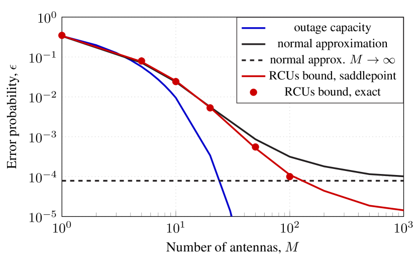
(a) Fixed average received $\text{SNR}=1\,\mathrm{dB}$.

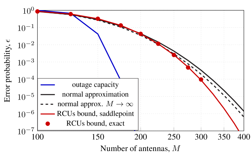
(b) Fixed transmit power $\rho=-24\,\mathrm{dBm}$.

Figure 1: Average error probability in the UL of a single-UE multiantenna system when $\widehat{g}=g=\lVert\bf h\rVert$ with ${\bf h}\sim\mathcal{CN}({\bf 0}_{M},\beta{\bf I}_{M})$, $n=100$, and $R=0.6$ bits per channel use. The UE is assumed to be at a distance from the BS that results in $\beta/\sigma^{2}=1$.

In Fig. 1, we depict the outage probability in (26) as a function of the number of BS antennas $M$. Comparisons are made with the upper bound in (5), evaluated by means of both Monte-Carlo integration (exact) and the saddlepoint approximation in Theorem 2. We also depict the normal approximation obtained by averaging (7) over $g$. In the evaluation of (5), we set $\widehat{g}=g$ and optimize over the parameter $s$ by means of a bisection search. We assume that $\sigma^{2}=-94\,\mathrm{dBm}$ and set $\beta=\sigma^{2}$ so that $\operatorname{\mathbb{E}}\mathopen{}\left[{g}^{2}\right]/\sigma^{2}=\beta M/\sigma^{2}=M$. Furthermore, we consider a codeword length $n=100$ and a rate of $R=60/100=0.6$ bits per channel use.

In Fig. 1(a), we illustrate the error probability for a transmit power $\rho$ that decreases as $1/M$. Specifically, we set $\rho=\widetilde{\rho}/M$ with $\widetilde{\rho}=1$ dB. Since ${g}^{2}/M\to\beta$ as $M\to\infty$ and we assume $\beta=\sigma^{2}$, it thus follows that the instantaneous SNR $\rho{g}^{2}/\sigma^{2}$ converges to the deterministic value $\widetilde{\rho}$ as $M\to\infty$. This means that, as $M\to\infty$, the normal approximation for i.i.d. Gaussian inputs given in (7) for a fixed $g$ converges to a deterministic quantity. Specifically, in the limit $M\to\infty$, we have that $I_{s}=\log(1+\widetilde{\rho}\beta/\sigma^{2})$ (achieved for $s=1/\sigma^{2}$) and $V_{s}=2\widetilde{\rho}\beta/(\widetilde{\rho}\beta+\sigma^{2})$ [29, Eq. (2.55)]. The resulting approximation is of interest because it does not require any Monte-Carlo averaging over the realizations of the fading channel. From Fig. 1(a), we see that the outage probability (26) approximates well the exact RCUs bound (5) only when $M$ is small, i.e., $M<5$, whereas the normal approximation loses accuracy when $M>20$. Both approximations are not accurate at the low error probabilities of interest in URLLC. The saddlepoint approximation is instead very accurate for all $M$ values.

In Fig. 1(b) we report the error probability with no power scaling so that the average received SNR increases as $M$ increases. Specifically, we consider a fixed transmit power $\rho=-24\,\mathrm{dBm}$. Hence, for $M=320$ the average received SNR in Fig. 1(b) equals $1\,\mathrm{dB}$, which coincides with the average received SNR in Fig. 1(a). With no power scaling, the outage probability (26) is an accurate approximation for the RCUs bound (5) only for very large values of the error probability, whereas the accuracy of the normal approximation (7) is acceptable for $\epsilon$ within the range $[10^{-3},1]$. The saddlepoint approximation again is on top of the RCUs bound for all values of error probability considered in the figure.

Based on the above results, we conclude that outage probability and the normal approximation do not always provide accurate estimates of the error probability achievable in large-antenna systems with short-packet communications over quasi-static channels. The accuracy of these approximations becomes even more questionable in the presence of imperfect CSI. This problem can be avoided altogether by using the nonasymptotic bound (5) in Theorem 1, which can be efficiently evaluated by means of the saddlepoint approximation in Theorem 2. In the next two sections, we will show how the simple input-output relation (1) can be used as building block for the analysis of practical Massive MIMO networks with imperfect CSI, pilot contamination, spatial correlation among antennas, and both inter-cell and intra-cell interference. Theorem 1 and Theorem 2 will then be used to efficiently evaluate the average error probability also in these more realistic scenarios.

III A Two-UE Single-Cell Massive MIMO Scenario

We consider a single-cell network where the BS is equipped with $M$ antennas and serves $K=2$ single-antenna UEs. We denote by $\mathbf{h}_{i}\in\mathbb{C}^{M}$ the channel vector between the BS and UE $i$ for $i=1,2$. We use a correlated Rayleigh fading model where $\mathbf{h}_{i}\sim\mathcal{CN}({\bf 0}_{M},{\bf R}_{i})$ remains constant for the duration of a codeword transmission. The normalized trace $\beta_{i}=\mathrm{tr}({\bf{R}}_{i})/M$ determines the average large-scale fading between UE $i$ and the BS, while the eigenstructure of ${\bf{R}}_{i}$ describes its spatial channel correlation [11, Sec. 2.2]. We assume that ${\bf{R}}_{1}$ and ${\bf{R}}_{2}$ are known at the BS; see, e.g., [33, 26] for a description of practical estimation methods. This setup is sufficient to demonstrate the usefulness of the framework developed in Section II for the analysis and design of Massive MIMO networks. A more general setup will be considered in Section IV.

III-A Uplink pilot transmission

We consider the standard time-division duplex (TDD) Massive MIMO protocol, where the UL and DL transmissions are assigned $n$ channel uses in total, divided in $n_{\text{{}p}}$ channel uses for UL pilots, $n_{\text{{}ul}}$ channel uses for UL data, and $n_{\text{{}dl}}=n-n_{\text{{}p}}-n_{\text{{}ul}}$ channel uses for DL data. We assume that the $n_{\text{{}p}}$-length pilot sequence $\bm{\phi}_{i}\in\mathbb{C}^{n_{\text{{}p}}}$ with $\bm{\phi}_{i}^{\mbox{\tiny$\mathrm{H}$}}\bm{\phi}_{i}=n_{\text{{}p}}$ is used by UE $i$ for channel estimation. The elements of $\bm{\phi}_{i}$ are scaled by the square-root of the pilot power $\sqrt{\rho^{\mathrm{ul}}}$ and transmitted over $n_{\text{{}p}}$ channel uses. When the UEs transmit their pilot sequences, the received pilot signal ${\bf Y}^{\mathrm{pilot}}\in\mathbb{C}^{M\times n_{\text{{}p}}}$ is

$${\bf Y}^{\mathrm{pilot}}=\sqrt{\rho^{\mathrm{ul}}}\mathbf{h}_{1}\bm{\phi}_{1}^{\mbox{\tiny$\mathrm{H}$}}+\sqrt{\rho^{\mathrm{ul}}}\mathbf{h}_{2}\bm{\phi}_{2}^{\mbox{\tiny$\mathrm{H}$}}+{\bf Z}^{\mathrm{pilot}}$$ (27)

where ${\bf Z}^{\mathrm{pilot}}\in\mathbb{C}^{M\times n_{\text{{}p}}}$ is the additive noise with i.i.d. elements distributed as $\mathcal{CN}(0,\sigma_{\mathrm{ul}}^{2})$. Assuming that $\mathbf{R}_{1}$ and $\mathbf{R}_{2}$ are known at the BS, the MMSE estimate of $\mathbf{h}_{i}$ is [11, Sec. 3.2]

$$\widehat{\mathbf{h}}_{i}=\sqrt{\rho^{\mathrm{ul}}n_{\text{{}p}}}{\bf R}_{i}{\bf Q}_{i}^{-1}\left({\bf Y}^{\mathrm{pilot}}\bm{\phi}_{i}\right)$$ (28)

for $i=1,2$ with

$${\bf Q}_{i}=\rho^{\mathrm{ul}}{\bf R}_{1}\bm{\phi}_{1}^{\mbox{\tiny$\mathrm{H}$}}\bm{\phi}_{i}+\rho^{\mathrm{ul}}{\bf R}_{2}\bm{\phi}_{2}^{\mbox{\tiny$\mathrm{H}$}}\bm{\phi}_{i}+\sigma_{\mathrm{ul}}^{2}{\bf I}_{M}.$$ (29)

The MMSE estimate $\widehat{\mathbf{h}}_{i}$ and the estimation error $\widetilde{\mathbf{h}}_{i}={\mathbf{h}}_{i}-\widehat{\mathbf{h}}_{i}$ are independent random vectors, distributed as $\widehat{\mathbf{h}}_{i}\sim\mathcal{CN}({\bf 0},{\bf\Phi}_{i})$ and $\widetilde{\mathbf{h}}_{i}\sim\mathcal{CN}({\bf 0},{\bf R}_{i}-{\bf\Phi}_{i})$, respectively, with ${\bf\Phi}_{i}={\rho^{\mathrm{ul}}n_{\text{{}p}}}{\bf R}_{i}{\bf Q}_{i}^{-1}{\bf R}_{i}$.

It follows from (29) that if the two UEs use orthogonal pilot sequences, i.e., $\bm{\phi}_{1}^{\mathsf{H}}\bm{\phi}_{2}=0$, they do not interfere, whereas they interfere if they use the same pilot sequence, i.e. $\bm{\phi}_{1}=\bm{\phi}_{2}$. This interference is known as pilot contamination and has two main consequences in the channel estimation process [11, Sec. 3.2.2]. The first is a reduced estimation quality; the second is that the estimates $\widehat{\mathbf{h}}_{1}$ and $\widehat{\mathbf{h}}_{2}$ become correlated. To see this, observe that if $\bm{\phi}_{1}=\bm{\phi}_{2}$ then ${\bf Y}^{\mathrm{pilot}}\bm{\phi}_{1}={\bf Y}^{\mathrm{pilot}}\bm{\phi}_{2}$ and ${\bf Q}_{1}={\bf Q}_{2}={\bf Q}$ with ${\bf Q}=\rho^{\mathrm{ul}}n_{\text{{}p}}{\bf R}_{1}+\rho^{\mathrm{ul}}n_{\text{{}p}}{\bf R}_{2}+\sigma_{\mathrm{ul}}^{2}{\bf I}_{M}$. Hence, $\widehat{\mathbf{h}}_{2}$ can be written as $\widehat{\mathbf{h}}_{2}={\bf R}_{2}\left({\bf R}_{1}\right)^{-1}\widehat{\mathbf{h}}_{1}$ provided that ${\bf R}_{1}$ is invertible. This implies that the two estimates are correlated with cross-correlation matrix given by $\operatorname{\mathbb{E}}\mathopen{}\left[\widehat{\mathbf{h}}_{1}\widehat{\mathbf{h}}_{2}^{\mbox{\tiny$\mathrm{H}$}}\right]={\bf\Upsilon}_{12}=\rho^{\mathrm{ul}}n_{\text{{}p}}{\bf R}_{1}{\bf Q}^{-1}{\bf R}_{2}$. This holds even though the underlying channels ${\bf h}_{1}$ and ${\bf h}_{2}$ are statistically independent, which implies that $\operatorname{\mathbb{E}}\mathopen{}\left[{\mathbf{h}}_{1}{\mathbf{h}}_{2}^{\mbox{\tiny$\mathrm{H}$}}\right]={\bf 0}_{M}$. Observe that if there is no spatial correlation, i.e., ${\bf R}_{i}=\beta_{i}{\bf I}_{M}$, $i=1,2$, then the channel estimates are identical up to a scaling factor, i.e., they are linearly dependent. We will return to the issue of pilot contamination in Section III-E.

III-B Uplink data transmission

During UL data transmission, the received complex baseband signal $\mathbf{r}^{\mathrm{ul}}[k]\in\mathbb{C}^{M}$ over an arbitrary channel use $k$, where $k=1,\ldots,n_{\text{{}ul}}$, is given by

$$\mathbf{r}^{\mathrm{ul}}[k]=\mathbf{h}_{1}x_{1}^{\mathrm{ul}}[k]+\mathbf{h}_{2}x_{2}^{\mathrm{ul}}[k]+\mathbf{z}^{\mathrm{ul}}[k]$$ (30)

where $x_{i}^{\mathrm{ul}}[k]\sim\mathcal{CN}(0,\rho^{\mathrm{ul}})$ is the information bearing signal transmitted by UE $i$ with $\rho^{\mathrm{ul}}$ being the average UL transmit power and $\mathbf{z}^{\mathrm{ul}}[k]\sim\mathcal{CN}({\bf 0},\sigma_{\mathrm{ul}}^{2}{\bf I}_{M})$ is the independent additive noise. The BS detects the signal $x_{1}^{\mathrm{ul}}[k]$ by using the combining vector ${\bf u}_{1}\in\mathbb{C}^{M}$, to obtain

$$y_{1}^{\mathrm{ul}}[k] = {\bf u}^{\mathsf{H}}_{1}\mathbf{r}^{\mathrm{ul}}[k]$$ (31)

$$= {\bf u}^{\mathsf{H}}_{1}\mathbf{h}_{1}x_{1}^{\mathrm{ul}}[k]+{\bf u}^{\mathsf{H}}_{1}\mathbf{h}_{2}x_{2}^{\mathrm{ul}}[k]+{\bf u}^{\mathsf{H}}_{1}\mathbf{z}^{\mathrm{ul}}[k].$$

Note that (31) has the same form as (1) with $v[k]=y_{1}^{\mathrm{ul}}[k]$, $q[k]=x_{1}^{\mathrm{ul}}[k]$, $g={\bf u}^{\mathsf{H}}_{1}\mathbf{h}_{1}$, and $z[k]={\bf u}^{\mathsf{H}}_{1}\mathbf{h}_{2}x_{2}^{\mathrm{ul}}[k]+{\bf u}^{\mathsf{H}}_{1}\mathbf{z}^{\mathrm{ul}}[k]$. Furthermore, given $\{{\bf h}_{1},{\bf u}_{1},{\bf h}_{2}\}$, the random variables $\{z[k]:k=1,\ldots,n_{\text{{}ul}}\}$ are conditionally i.i.d. and $z[k]\sim\mathcal{CN}(0,\sigma^{2})$ with $\sigma^{2}=\rho^{\mathrm{ul}}\lvert{\bf u}^{\mathsf{H}}_{1}\mathbf{h}_{2}\rvert^{2}+\lVert{\bf u}_{1}\rVert^{2}\sigma_{\text{{}ul}}^{2}$.

We assume that the BS treats the acquired (noisy) channel estimate $\widehat{\mathbf{h}}_{1}$ as perfect. This implies that, to recover the transmitted codeword, which we assume to be drawn from a codebook $\mathcal{C}^{\mathrm{ul}}$, it performs mismatched SNN decoding with $\widehat{g}={\bf u}^{\mathsf{H}}_{1}\widehat{\mathbf{h}}_{1}$. Specifically, the estimated codeword $\widehat{\bf x}_{1}^{\mathrm{ul}}$ is obtained as

$$\widehat{\bf x}_{1}^{\mathrm{ul}}=\operatorname*{arg\;min}_{\widetilde{\bf x}_{1}^{\mathrm{ul}}\in\mathcal{C}^{\mathrm{ul}}}\lVert{\bf y}_{1}^{\mathrm{ul}}-({\bf u}^{\mathsf{H}}_{1}\widehat{\mathbf{h}}_{1})\widetilde{\bf x}_{1}^{\mathrm{ul}}\rVert^{2}$$ (32)

with ${\bf y}_{1}^{\mathrm{ul}}=[y_{1}^{\mathrm{ul}}[1],\ldots,y_{1}^{\mathrm{ul}}[n_{\text{{}ul}}]]^{\mbox{\tiny$\mathrm{T}$}}$ and $\widetilde{\bf x}_{1}^{\mathrm{ul}}=[\widetilde{x}_{1}^{\mathrm{ul}}[1],\ldots,\widetilde{x}_{1}^{\mathrm{ul}}[n_{\text{{}ul}}]]^{\mbox{\tiny$\mathrm{T}$}}$. It thus follows that (3) provides a bound on the conditional error probability for UE $1$ given $g$ and $\widehat{g}$. To obtain the average error probability, we need to take an expectation over $g={\bf u}^{\mathsf{H}}_{1}\mathbf{h}_{1}$, $\widehat{g}={\bf u}^{\mathsf{H}}_{1}\widehat{\mathbf{h}}_{1}$, and $\sigma^{2}=\rho^{\mathrm{ul}}\lvert{\bf u}^{\mathsf{H}}_{1}\mathbf{h}_{2}\rvert^{2}+\lVert{\bf u}_{1}\rVert^{2}\sigma_{\text{{}ul}}^{2}$, which results in

$$\epsilon_{1}^{\mathrm{ul}}$$

$$\leq\operatorname{\mathbb{E}}\mathopen{}\left[\mathbb{P}\mathopen{}\left[{\sum_{k=1}^{n_{\text{{}ul}}}\imath_{s}(y_{1}^{\mathrm{ul}}[k],x_{1}^{\mathrm{ul}}[k])\leq\log\frac{m-1}{u}\Bigg{|}g,\widehat{g},\sigma^{2}}\right]\right].$$

(33)

The saddlepoint approximation in Theorem 2 can be applied verbatim to efficiently compute the conditional probability in (33). The average error probability for UE $2$ can be evaluated similarly.

The combining vector ${\bf u}_{1}$ is selected at the BS based on the channel estimates $\widehat{\bf h}_{1}$ and $\widehat{\bf h}_{2}$. The simplest choice is to use MR combining: ${\bf u}_{1}^{\rm{MR}}=\widehat{\mathbf{h}}_{1}/M$. A more computationally intensive choice is MMSE combining:

$${\bf u}_{1}^{\rm{MMSE}}=\left(\sum\limits_{i=1}^{2}\widehat{\mathbf{h}}_{i}\widehat{\mathbf{h}}_{i}^{\mbox{\tiny$\mathrm{H}$}}+{\bf Z}\right)^{-1}\widehat{\mathbf{h}}_{1}$$ (34)

where ${\bf Z}=\sum\nolimits_{i=1}^{2}{\bf\Phi}_{i}+\frac{\sigma_{\mathrm{ul}}^{2}}{\rho^{\mathrm{ul}}}{\bf{I}}_{M}$.

III-C Downlink data transmission

Assume that, to transmit to UE $i$ with $i=1,2$, the BS uses the precoding vector ${\bf w}_{i}\in\mathbb{C}^{M}$, which determines the spatial directivity of the transmission and satisfies the normalization $\operatorname{\mathbb{E}}\mathopen{}\left[\|{\mathbf{w}_{i}}\|^{2}\right]=1$. During DL data transmission, the received signal $y_{1}^{\mathrm{dl}}[k]\in\mathbb{C}$ at UE $1$ over channel use $k$, where $k=1,\ldots,n_{\text{{}dl}}$, is

$$y_{1}^{\mathrm{dl}}[k]=\mathbf{h}^{\mathsf{H}}_{1}{\bf w}_{1}x_{1}^{\mathrm{dl}}[k]+\mathbf{h}^{\mathsf{H}}_{1}{\bf w}_{2}x_{2}^{\mathrm{dl}}[k]+z_{1}^{\mathrm{dl}}[k]$$ (35)

where $x_{i}^{\mathrm{dl}}[k]\sim\mathcal{CN}(0,\rho^{\mathrm{dl}})$ is the data signal intended for UE $i$ and $z_{1}^{\mathrm{dl}}[k]\sim\mathcal{CN}(0,\sigma_{\mathrm{dl}}^{2})$ is the receiver noise at UE $1$. Again, we can put (35) in the same form as (1) by setting $v[k]=y_{1}^{\mathrm{dl}}[k]$, $q[k]=x_{1}^{\mathrm{dl}}[k]$, $g=\mathbf{h}^{\mathsf{H}}_{1}{\bf w}_{1}$ and $z[k]=\mathbf{h}^{\mathsf{H}}_{1}{\bf w}_{2}x_{2}^{\mathrm{dl}}[k]+z_{1}^{\mathrm{dl}}[k]$. Note that, given $\{{\bf h}_{1},{\bf w}_{1},{\bf w}_{2}\}$, the random variables $\{z[k]:k=1,\ldots,n_{\text{{}dl}}\}$ are conditional i.i.d. and $z[k]\sim\mathcal{CN}(0,\sigma^{2})$ with $\sigma^{2}=\rho^{\mathrm{dl}}\lvert\mathbf{h}^{\mathsf{H}}_{1}{\bf w}_{2}\rvert^{2}+\sigma_{\text{{}dl}}^{2}$.

Since no pilots are transmitted in the DL, the UE does not know the precoded channel $g=\mathbf{h}^{\mathsf{H}}_{1}{\bf w}_{1}$ in (35). Instead, we assume that the UE has access its expected value $\operatorname{\mathbb{E}}\mathopen{}\left[\mathbf{h}^{\mathsf{H}}_{1}{\bf w}_{1}\right]$ and uses this quantity to perform mismatched SNN decoding. Specifically, we have that $\widehat{g}=\operatorname{\mathbb{E}}\mathopen{}\left[\mathbf{h}^{\mathsf{H}}_{1}{\bf w}_{1}\right]$ and

$$\widehat{\bf x}_{1}^{\mathrm{dl}}=\operatorname*{arg\;min}_{\widetilde{\bf x}_{1}^{\mathrm{dl}}\in\mathcal{C}^{\mathrm{dl}}}\lVert{\bf y}_{1}^{\mathrm{dl}}-\widehat{g}\widetilde{\bf x}_{1}^{\mathrm{dl}}\rVert^{2}$$ (36)

with ${\bf y}_{1}^{\mathrm{dl}}=[y_{1}^{\mathrm{dl}}[1],\ldots,y_{1}^{\mathrm{dl}}[n_{\text{{}dl}}]]^{\mbox{\tiny$\mathrm{T}$}}$ and $\widetilde{\bf x}_{1}^{\mathrm{dl}}=[\widetilde{x}_{1}^{\mathrm{dl}}[1],\ldots,\widetilde{x}_{1}^{\mathrm{dl}}[n_{\text{{}dl}}]]^{\mbox{\tiny$\mathrm{T}$}}$. Obviously, channel hardening is critical for this choice to result in good performance [11, Sec. 2.5.1]. Since $\widehat{g}=\operatorname{\mathbb{E}}\mathopen{}\left[\mathbf{h}^{\mathsf{H}}_{1}{\bf w}_{1}\right]$ is deterministic, the error probability at UE $1$ in the DL can be evaluated as follows:

$$\epsilon_{1}^{\mathrm{dl}}\leq\operatorname{\mathbb{E}}\mathopen{}\left[\mathbb{P}\mathopen{}\left[{\sum_{k=1}^{n_{\text{{}dl}}}\imath_{s}(y_{1}^{\mathrm{dl}}[k],x_{1}^{\mathrm{dl}}[k])\leq\log\frac{m-1}{u}\Bigg{|}g,\sigma^{2}}\right]\right].$$

(37)

Similarly to (33), the saddlepoint approximation in Theorem 2 can be used to evaluate the conditional probability in (37) efficiently.

Similar to the UL, the upper bound (37) holds for any precoder vector that is selected on the basis of the channel estimates available at the BS. Different precoders yield different tradeoffs between the error probability achievable at the UEs. A common heuristic comes from UL-DL duality [11, Sec. 4.3.2], which suggests to choose the precoding vectors ${\bf w}_{i}$ as the following function of the combining vectors: ${\bf w}_{i}={{\bf u}_{i}}/{\sqrt{\operatorname{\mathbb{E}}\mathopen{}\left[\lVert{\bf u}_{i}\rVert^{2}\right]}}$. By selecting ${\bf u}_{i}$ as one of the uplink combining schemes described earlier, the corresponding precoding scheme is obtained; that is, ${\bf u}_{i}={\bf u}_{i}^{\rm{MR}}$ yields MR precoding and ${\bf u}_{i}={\bf u}_{i}^{\rm{MMSE}}$ yields MMSE precoding.

III-D Numerical Analysis

In this section, we use the finite blocklength bound in Theorem 1 to study the impact of imperfect CSI, pilot contamination, and spatial correlation in both UL and DL. We assume that the $K=2$ UEs are within a square area of $75\,\text{m}\times 75\,\text{m}$, with the BS at the center of the square. The BS is equipped with a horizontal uniform linear array (ULA) with antenna elements separated by half a wavelength. The antennas and the UEs are located in the same horizontal plane, thus the azimuth angle is sufficient to determine the directivity. We assume that the scatterers are uniformly distributed in the angular interval $[\varphi_{i}-\Delta,\varphi_{i}+\Delta]$, where $\varphi_{i}$ is the nominal angle-of-arrival (AoA) of UE $i$ and $\Delta$ is the angular spread. Hence, the $(m_{1},m_{2})$th element of ${\bf R}_{i}$ is equal to [11, Sec. 2.6]

$$\left[{\bf R}_{i}\right]_{m_{1},m_{2}}=\frac{\beta_{i}}{2\Delta}\int_{-\Delta}^{\Delta}{e^{\mathsf{j}\pi(m_{1}-m_{2})\sin(\varphi_{i}+{\bar{\varphi}})}}d{\bar{\varphi}}.$$ (38)

We assume $\Delta=25^{\circ}$ and let the large-scale fading coefficient, measured in $\,\mathrm{dB}$, be

$$\beta_{i}\,=-35.3-37.6\log_{10}\left(\frac{d_{i}}{1\,\text{m}}\right)$$ (39)

where $d_{i}$  is the distance between the BS and UE $i$. The communication takes place over a $20$ MHz bandwidth with a total receiver noise power of $\sigma_{\mathrm{ul}}^{2}=\sigma_{\mathrm{dl}}^{2}=-94$ dBm (consisting of thermal noise and a noise figure of $7$ dB in the receiver hardware) at both the BS and UEs. The UL and DL transmit powers are equal and given by $\rho^{\mathrm{ul}}=\rho^{\mathrm{dl}}=10\,\text{mW}$. We assume a total of $n=300$ channel uses, out of which $n_{\text{{}p}}$ channel uses are allocated for pilot transmission and $n_{\text{{}ul}}=n_{\text{{}dl}}=(n-n_{\text{{}p}})/2$ channel uses are assigned to the UL and DL data transmissions, respectively. In each data-transmission phase, $b=160$ information bits are to be conveyed. These parameters are in agreement with the stringent low-latency setups described in [3, App. A.2.3.1].

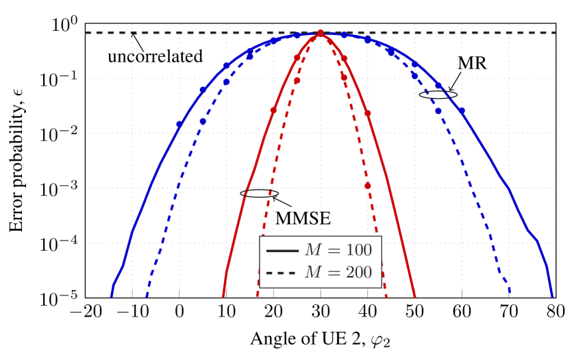
(a) Uplink transmission.

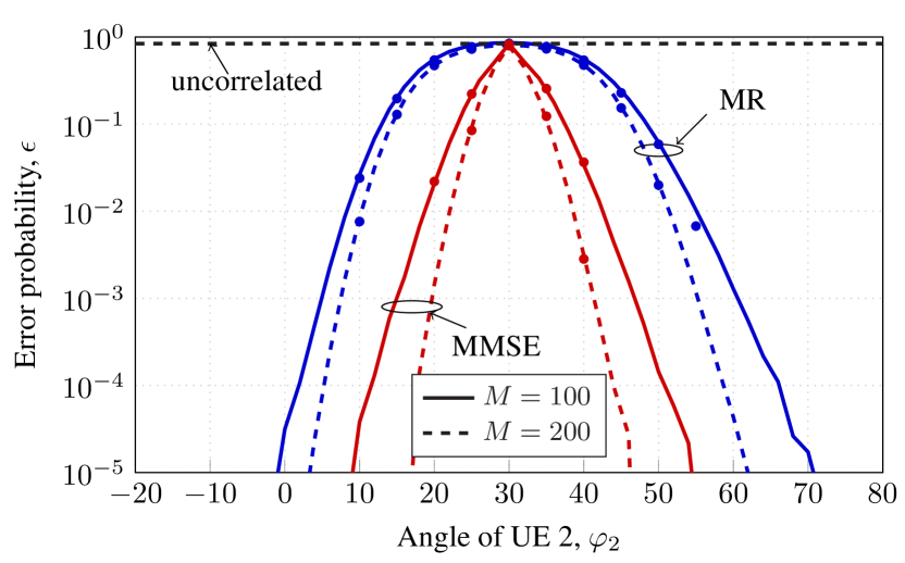
(b) Downlink transmission.

Figure 2: Average error probability $\epsilon$ for UE $1$ versus the nominal angle of UE $2$ when $\bm{\phi}_{1}=\bm{\phi}_{2}$. Here, $\rho^{\text{ul}}=\rho^{\text{dl}}=10$ $\,\mathrm{dB}$m, $\Delta=25^{\circ}$, $\varphi_{1}=30^{\circ}$, $b=160$, $n_{\text{{}p}}=2$, and $n=300$. The curves are obtained using the saddlepoint approximation; the circles indicate the values of the RCUs bound, computed directly via (5).

Fig. 2 shows the UL and DL error probability $\epsilon$ of UE $1$ with MR and MMSE combining, when the two UEs use the same pilot sequence (i.e., pilot contamination is present) and $M=100$ or $200$. The uncorrelated Rayleigh-fading case where ${\bf R}_{i}=\beta_{i}{\bf I}_{M}$, $i=1,2$, is also reported as reference. The nominal angle of UE $1$ is fixed at $\varphi_{1}=30^{\circ}$ while the angle of UE $2$ varies from $-20^{\circ}$ to $80^{\circ}$. We let $d_{1}=d_{2}=36.4$ m, which leads to $\beta_{1}=\beta_{2}=-94\,\mathrm{dB}$. Fig. 2 reveals that a low error probability can be achieved if the UEs are well-separated in the angle domain, even when the channel estimates are affected by pilot contamination. MMSE combining/precoding achieves a much lower error probability for a given angle separation. These results are in agreement with the findings reported in the asymptotic regime of large packet size in [26, 6].

Fig. 2 shows that the error probability with MR combining in the UL is worse than that of MR precoding in the DL. This phenomenon can be clarified by comparing the input-otput relations in (31) and (35) for the case of perfect CSI at both BS and UEs. Specifically, when the desired signal experiences a deep fade, the magnitude of the UL interference is unaffected whereas the DL interference becomes small. This results in a larger error probability in the UL compared to the DL. The same argument holds also for the case of imperfect CSI with and without pilot contamination. Note that this phenomenon does not occur when MMSE combining/precoding is used. On the contrary, with MMSE combining/precoding the DL performs slightly worse than the UL because DL decoding relies on channel hardening.

Assume now that the $2$ UEs are positioned independently and uniformly at random within the square area of $75\,\text{m}\times 75\,\text{m}$, with a minimum distance from the BS of $5\,\text{m}$. Fig. 3 shows the UL and DL network availability $\eta$ with both MR and MMSE when $M=100$. We define $\eta$ as

$$\eta=\mathbb{P}\mathopen{}\left[{\epsilon\leq\epsilon_{\text{{}target}}}\right]$$ (40)

and represents the probability that the target error probability $\epsilon_{\text{{}target}}$ is achieved on a link between a randomly positioned UE and its corresponding BS, in the presence of randomly positioned interfering UEs (in this case, just one). Note that the error probability $\epsilon$ is averaged with respect to the small-scale fading and the additive noise, given the UEs location, whereas the network availability is computed with respect to the random UEs locations. We consider both the scenario in which the UEs use orthogonal pilot sequences, i.e., $\bm{\phi}_{1}^{\mbox{\tiny$\mathrm{H}$}}\bm{\phi}_{2}=0$, and the one in which $\bm{\phi}_{1}=\bm{\phi}_{2}$.

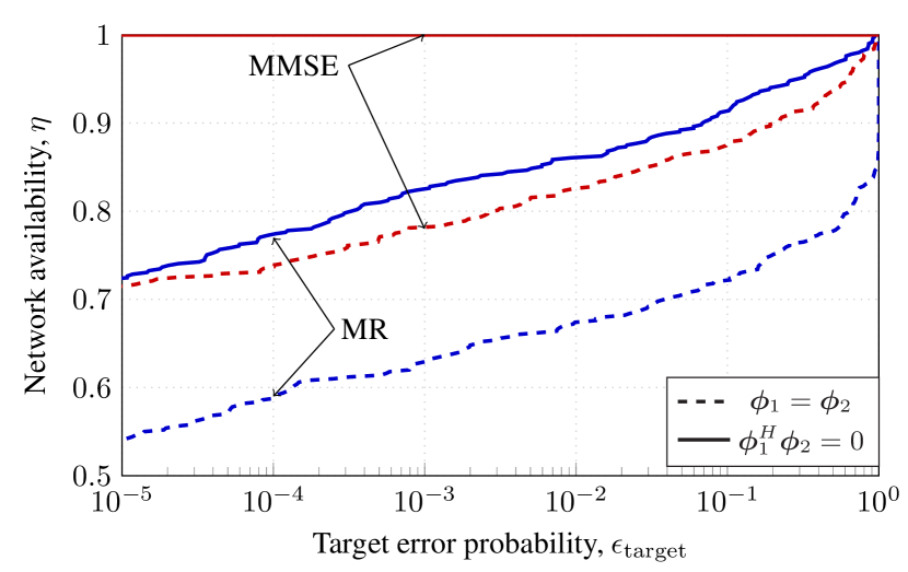
(a) Uplink transmission.

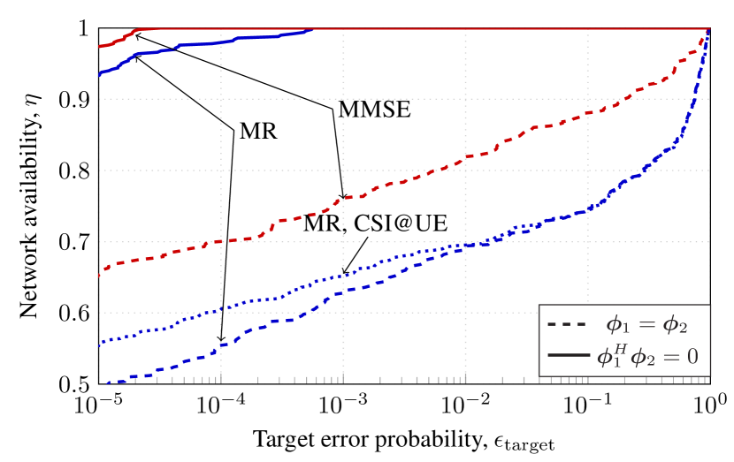
(b) Downlink transmission.

Figure 3: Network availability $\eta$ with and without pilot contamination with $M=100$, $\rho^{\mathrm{ul}}=\rho^{\mathrm{dl}}=10$ $\,\mathrm{dBm}$, $n_{\text{{}p}}=2$, $b=160$, $n=300$, and $\Delta=25^{\circ}$.

The results of Fig. 3 show that pilot contamination reduces significantly the network availability irrespective of the processing scheme. MR performs better in the DL than in the UL when orthogonal pilot sequences are used. This is in agreement with what stated when discussing Fig. 2. However, in the case of pilot contamination, the UL achieves better performance than the DL when the UE relies on channel hardening (and slightly worse performance than the DL when the UE has access to perfect CSI). Note that this does not contradict what stated after Fig. 2. Indeed, due to the random UE placements, the correlation matrix may have low rank. This affects channel hardening and, consequently, results in a deterioration of the DL performance. For MMSE processing, the UL is always superior to the DL because the DL relies on channel hardening.

III-E Asymptotic Analysis as $M\to\infty$

It is well known that, for spatially uncorrelated Rayleigh fading channels, the interference caused by pilot contamination limits the spectral efficiency of Massive MIMO in the large-blocklength ergodic setup as $M\to\infty$ and the number of UEs $K$ is fixed, for both MR and MMSE combining/precoding [4, 34]. However, it was recently shown in [6] that Massive MIMO with MMSE combining/precoding is not asymptotically limited by pilot contamination when the spatial correlation exhibited by practically relevant channels is taken into consideration.

We show next that a similar conclusion holds for the average error probability in the finite-blockength regime when $M\to\infty$ and $K=2$. Specifically, we prove that, in the presence of spatial correlation, the error probability vanishes as $M\to\infty$, provided that MMSE combining/precoding is used. To this end, we will proceed similarly as in [6] and make the following two assumptions.

Assumption 1

For $i=1,2$, $\liminf_{M}\frac{1}{M}\mathrm{tr}\mathopen{}\left({{\bf R}_{i}}\right)>0$ and $\limsup_{M}\lVert\bm{R}_{i}\rVert_{2}<\infty$.

Assumption 2

For $(\lambda_{1},\lambda_{2})\in\use@mathgroup\M@U\symAMSb{R}^{2}$ and $i=1,2$,

$$\liminf_{M}\inf_{\mathopen{}\left\{{(\lambda_{1},\lambda_{2}):\lambda_{i}=1}\right\}}\frac{1}{M}\lVert\lambda_{1}{\bf R}_{1}+\lambda_{2}{\bf R}_{2}\rVert_{F}^{2}>0.$$ (41)

The first condition in Assumption 1 implies that the array gathers an amount of signal energy that is proportional to $M$. The second condition implies that the increased signal energy is spread over many spatial dimensions, i.e., the rank of ${\bf R}_{i}$ must be proportional to $M$. These two conditions are commonly invoked in the asymptotic analysis of Massive MIMO [34]. Assumption 2 requires ${\bf R}_{1}$ and ${\bf R}_{2}$ to be asymptotically linearly independent [26].

In Theorem 3 below, we establish that, with MR combining, the probability of error vanishes as $M\to\infty$ if the two UEs transmit orthogonal pilot sequences. However, it converges to a positive constant if they share the same pilot sequence.

Theorem 3

Let $c>0$ be a positive real-valued scalar. If MR combining is used with ${\bf u}_{1}^{\rm{MR}}=\frac{1}{M}\widehat{\mathbf{h}}_{1}$, then under Assumption 1,

$$\lim_{M\to\infty}\epsilon_{1}^{\mathrm{ul}} = 0,\text{ if }\bm{\phi}_{1}^{\mbox{\tiny$\mathrm{H}$}}\bm{\phi}_{2}=0,$$ (42)

$$\lim_{M\to\infty}\epsilon_{1}^{\mathrm{ul}} = c,\text{ if }\bm{\phi}_{1}=\bm{\phi}_{2}.$$ (43)

Proof:

See Appendix C. ∎

Next, we show that, if MMSE combining is used, the error probability vanishes as $M\to\infty$ even in the presence of pilot contamination.

Theorem 4

If MMSE combining is used with ${\bf u}_{1}^{\rm{MMSE}}$ given by (34), then under Assumption 1 and Assumption 2, the average error probability $\epsilon_{1}^{\mathrm{ul}}$ goes to zero as $M\rightarrow\infty$, both when $\bm{\phi}_{1}^{\mbox{\tiny$\mathrm{H}$}}\bm{\phi}_{2}=0$ and when $\bm{\phi}_{1}=\bm{\phi}_{2}$.

Proof:

The proof is given in Appendix D. It makes use of the asymptotic analysis presented in [6, App. B] to show that $y_{1}^{\text{ul}}\asymp x_{1}^{\text{ul}}$ as $M\to\infty$, even in the presence of pilot contamination. Once this is proved, the result follows by applying Lemma 1 from Section II. ∎

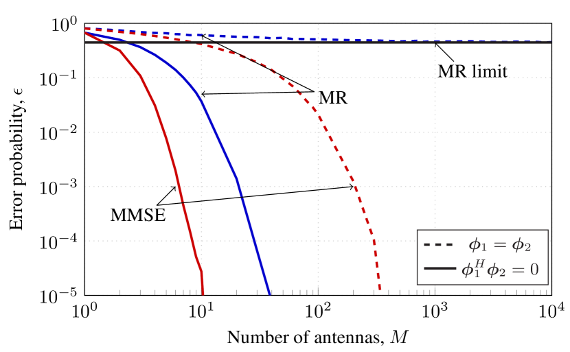
(a) Uplink transmission.

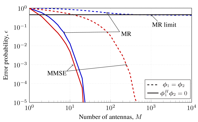
(b) Downlink transmission.

Figure 4: Average error probability $\epsilon$ of UE $1$ versus number of antennas $M$ with and without pilot contamination. Here, $\rho^{\mathrm{ul}}=\rho^{\mathrm{dl}}=10$ $\,\mathrm{dBm}$, $n_{\text{{}p}}=2$, $b=160$, $n=300$, $\Delta=25^{\circ}$, $\varphi_{1}=30^{\circ}$, and $\varphi_{2}=40^{\circ}$.

Note that Theorem 3 and Theorem 4 can be extended to the DL with a similar methodology. Details are omitted due to space limitations.

To validate the asymptotic analysis provided by Theorems 3 and 4 and to quantify the impact of pilot contamination for values of $M$ of practical interest, we numerically evaluate the UL error probability when the $2$ UEs transmit at the same power, are at the same distance from the BS, and use the same pilot sequence. Furthermore, we assume that their nominal angles are $\varphi_{1}=30^{\circ}$ and $\varphi_{2}=40^{\circ}$. Note that the angle between the two UEs is small. Hence, we expect pilot contamination to have a significant impact on the error probability. As in Fig. 2, we assume that $\sigma_{\text{{}ul}}^{2}=\sigma_{\text{{}dl}}^{2}=-94\,\mathrm{dBm}$ and that the UEs are located $36.4$ m away from the BS so that $\beta_{1}=\beta_{2}=-94\,\mathrm{dB}$. In Fig. 4(a), we illustrate the average error probability as a function of $M$ with MR and MMSE. We see that, in the presence of pilot contamination, the error probability with MR converges to a nonzero constant as $M$ grows, in accordance with Theorem 3. In contrast, the error probability with MMSE goes to $0$ as $M\to\infty$, in accordance with Theorem 4. However, a comparison with the orthogonal-pilot case reveals that, for fixed $M$, pilot contamination has a significant impact on the error probability of MMSE. As shown in Fig. 4(b), similar conclusions can be drawn for the DL.

IV Massive MIMO Network

We will now extend the analysis in Section III to a Massive MIMO network with $L$ cells, each comprising a BS with $M$ antennas and $K$ UEs. We denote by ${\mathbf{h}}_{li}^{j}\sim\mathcal{CN}({\mathbf{0}}_{M},{\bf R}_{li}^{j})$ the channel between UE $i$ in cell $l$ and the BS in cell $j$. The $n_{\text{{}p}}$-length pilot sequence of UE $i$ in cell $j$ is denoted by the vector $\bm{\phi}_{ji}\in\mathbb{C}^{n_{\text{{}p}}}$ and satisfies $\|\bm{\phi}_{ji}\|^{2}=n_{\text{{}p}}$. We assume that the $K$ UEs in a cell use mutually orthogonal pilot sequences and these pilot sequences are reused in a fraction $1/f$ of the $L$ cells with $n_{\text{{}p}}=Kf$. The channel vectors are estimated using the MMSE estimator given in [11, Sec. 3.2].

IV-A Uplink

The data signal from UE $i^{\prime}$ in cell $l$ over an arbitrary time instant $k$ is denoted by $x_{li^{\prime}}^{\rm ul}[k]\sim\mathcal{CN}({0},\rho^{\rm ul})$, with $\rho^{\rm ul}$ being the transmit power. To detect $x_{ji}^{\rm ul}[k]$, BS $j$ selects the combining vector ${\mathbf{u}}_{ji}\in\mathbb{C}^{M}$, which is multiplied with the received signal ${\mathbf{r}}_{j}^{\rm ul}[k]$ to obtain

$$\!\!y_{ji}^{\rm ul}[k] = {\mathbf{u}}_{ji}^{\mbox{\tiny$\mathrm{H}$}}{\mathbf{r}}_{j}^{\rm ul}[k]=\overbrace{\underbrace{\vphantom{\sum_{i^{\prime}=1,i^{\prime}\neq i}^{K}}{\mathbf{u}}_{ji}^{\mbox{\tiny$\mathrm{H}$}}{\mathbf{h}}_{ji}^{j}x_{ji}^{\rm ul}[k]}_{\textrm{Desired signal}}}^{gq[k]}+\overbrace{\underbrace{\sum_{i^{\prime}=1,i^{\prime}\neq i}^{K}{\mathbf{u}}_{ji}^{\mbox{\tiny$\mathrm{H}$}}{\mathbf{h}}_{ji^{\prime}}^{j}x_{ji^{\prime}}^{\rm ul}[k]}_{\textrm{Intra-cell interference}}}^{z[k]}$$ (44)

$${}+\overbrace{\underbrace{\sum_{l=1,l\neq j}^{L}\sum_{i^{\prime}=1}^{K}{\mathbf{u}}_{ji}^{\mbox{\tiny$\mathrm{H}$}}{\mathbf{h}}_{li^{\prime}}^{j}x_{li^{\prime}}^{\rm ul}[k]}_{\textrm{Inter-cell interference}}}^{z[k]}+\overbrace{\underbrace{\vphantom{\sum_{i^{\prime}=1,i^{\prime}\neq i}^{K}}{\mathbf{u}}_{ji}^{\mbox{\tiny$\mathrm{H}$}}{\mathbf{z}}_{j}^{\rm ul}[k]}_{\textrm{Noise}}}^{z[k]}$$

for $k=1,\ldots,n_{\text{{}ul}}$. We note that (44) can be put in the same form as (1) if we set $v[k]=y_{ji}^{\rm ul}[k]$, $q[k]=x_{ji}^{\rm ul}[k]$, $g={\mathbf{u}}_{ji}^{\mbox{\tiny$\mathrm{H}$}}{\mathbf{h}}_{ji}^{j}$, $\widehat{g}={\mathbf{u}}_{ji}^{\mbox{\tiny$\mathrm{H}$}}{\widehat{\mathbf{h}}}_{ji}^{j}$, and $z[k]=\sum_{i^{\prime}=1,i^{\prime}\neq i}^{K}{\mathbf{u}}_{ji}^{\mbox{\tiny$\mathrm{H}$}}{\mathbf{h}}_{ji^{\prime}}^{j}x_{ji^{\prime}}^{\rm ul}[k]+\sum_{l=1,l\neq j}^{L}\sum_{i^{\prime}=1}^{K}{\mathbf{u}}_{ji}^{\mbox{\tiny$\mathrm{H}$}}{\mathbf{h}}_{li^{\prime}}^{j}x_{li^{\prime}}^{\rm ul}[k]+{\mathbf{u}}_{ji}^{\mbox{\tiny$\mathrm{H}$}}{\mathbf{z}}_{j}^{\rm ul}[k]$. Given all channels and combining vectors, the random variables $\{z[k]:k=1,\ldots,n_{\text{{}ul}}\}$ are conditionally i.i.d. and $z[k]\sim\mathcal{CN}(0,\sigma^{2})$ with $\sigma^{2}=\sigma_{\text{{}ul}}^{2}\lVert\mathbf{u}_{ji}\rVert^{2}+\rho^{\mathrm{ul}}\sum_{i^{\prime}=1,i^{\prime}\neq i}^{K}\lvert\mathbf{u}^{\mathsf{H}}_{ji}\mathbf{h}_{ji^{\prime}}^{j}\rvert^{2}+\rho^{\mathrm{ul}}\sum_{l=1,l\neq j}^{L}\sum_{i^{\prime}=1}^{K}\lvert\mathbf{u}^{\mathsf{H}}_{ji}\mathbf{h}_{li^{\prime}}^{j}\rvert^{2}$. An upper bound on the error probability $\epsilon_{ji}^{\rm ul}$ then follows by applying (3) in Theorem 1 and then by averaging over $g$, $\widehat{g}$ and $\sigma^{2}$. This bound holds for any choice of ${\bf v}_{ji}$. In the numerical results, we will consider multicell MMSE and MR combining.

IV-B Downlink

The BS in cell $j$ transmits the DL signal ${\mathbf{x}}_{j}^{\rm dl}[k]=\sum_{ji^{\prime}=1}^{K}{\mathbf{w}}_{ji^{\prime}}x_{ji^{\prime}}^{\rm dl}[k]$ where $x_{ji^{\prime}}^{\rm dl}[k]\sim\mathcal{CN}(0,\rho^{\rm dl})$ is the DL data signal intended for UE $i^{\prime}$ in cell $j$ over the time index $k$, assigned to a precoding vector ${\mathbf{w}}_{ji^{\prime}}\in\mathbb{C}^{M}$ that satisfies $\|{\mathbf{w}}_{ji^{\prime}}\|^{2}=1$ so that $\rho^{\rm dl}$ represents the transmit power. The received signal $y_{ji}^{\rm dl}[k]\in\mathbb{C}$ for $k=1,\ldots,n_{\text{{}dl}}$ at UE $i$ in cell $j$ is given by

$$y_{ji}^{\rm dl}[k] = \overbrace{\underbrace{\vphantom{\sum_{i^{\prime}=1,i^{\prime}\neq i}^{K}}({\mathbf{h}}_{ji}^{j})^{\mbox{\tiny$\mathrm{H}$}}{\mathbf{w}}_{ji}x_{ji}^{\rm dl}[k]}_{\textrm{Desired signal}}}^{gq[k]}+\overbrace{\underbrace{\sum_{i^{\prime}=1,i^{\prime}\neq i}^{K}({\mathbf{h}}_{ji}^{j})^{\mbox{\tiny$\mathrm{H}$}}{\mathbf{w}}_{ji^{\prime}}x_{ji^{\prime}}^{\rm dl}[k]}_{\textrm{Intra-cell interference}}}^{z[k]}$$ (45)

$${}+\overbrace{\underbrace{\sum_{l=1,l\neq j}^{L}\sum_{i^{\prime}=1}^{K}({\mathbf{h}}_{ji}^{l})^{\mbox{\tiny$\mathrm{H}$}}{\mathbf{w}}_{li^{\prime}}x_{li^{\prime}}^{\rm dl}[k]}_{\textrm{Inter-cell interference}}}^{z[k]}+\overbrace{\underbrace{\vphantom{\sum_{i^{\prime}=1,i^{\prime}\neq i}^{K}}z_{ji}^{\rm dl}[k]}_{\textrm{Noise}}}^{z[k]}$$

where $z_{ji}^{\rm dl}[k]\sim\mathcal{CN}(0,\sigma_{\text{{}dl}}^{2})$ is the receiver noise. The desired signal to UE $i$ in cell $j$ propagates over the precoded channel $g_{ji}=({\mathbf{h}}_{ji}^{j})^{\mbox{\tiny$\mathrm{H}$}}{\mathbf{w}}_{ji}$. The UE does not know $g_{ji}$ and relies on channel hardening to approximate it with its mean value $\operatorname{\mathbb{E}}\mathopen{}\left[g_{ji}\right]=\operatorname{\mathbb{E}}\mathopen{}\left[({\mathbf{h}}_{ji}^{j})^{\mbox{\tiny$\mathrm{H}$}}{\mathbf{w}}_{ji}\right]$. As in the UL, we note that (45) can be put in the same form as (1) if we set $v[k]=y_{ji}^{\rm dl}[k]$, $q[k]=x_{ji}^{\rm dl}[k]$, $g=({\mathbf{h}}_{ji}^{j})^{\mbox{\tiny$\mathrm{H}$}}{\mathbf{w}}_{ji}$, $\widehat{g}=\operatorname{\mathbb{E}}\mathopen{}\left[({\mathbf{h}}_{ji}^{j})^{\mbox{\tiny$\mathrm{H}$}}{\mathbf{w}}_{ji}\right]$, and $z[k]=\sum_{i^{\prime}=1,i\neq i}^{K}({\mathbf{h}}_{ji}^{j})^{\mbox{\tiny$\mathrm{H}$}}{\mathbf{w}}_{ji^{\prime}}x_{ji^{\prime}}^{\rm dl}[k]+\sum_{l=1,l\neq j}^{L}\sum_{i^{\prime}=1}^{K}({\mathbf{h}}_{ji}^{l})^{\mbox{\tiny$\mathrm{H}$}}{\mathbf{w}}_{li^{\prime}}x_{li^{\prime}}^{\rm dl}[k]+z_{ji}^{\rm dl}[k]$. Given all channels and precoding vectors, the random variables $\{z[k]:k=1,\ldots,n_{\text{{}dl}}\}$ are conditionally i.i.d. and $z[k]\sim\mathcal{CN}(0,\sigma^{2})$ with $\sigma^{2}=\sigma_{\text{{}dl}}^{2}+\rho^{\mathrm{dl}}\sum_{i^{\prime}=1,i\neq i^{\prime}}^{K}\lvert(\mathbf{h}_{ji}^{j})^{\mathsf{H}}\mathbf{w}_{ji^{\prime}}\rvert^{2}+\rho^{\mathrm{dl}}\sum_{l=1,l\neq j}^{L}\sum_{i^{\prime}=1}^{K}\lvert(\mathbf{h}_{ji}^{l})^{\mathsf{H}}\mathbf{w}_{li^{\prime}}\rvert^{2}$. An upper bound on the error probability $\epsilon_{ji}^{\rm dl}$ then follows by applying (3) in Theorem 1 and then by averaging over $g$ and $\sigma^{2}$. As for the UL, the above results hold for any choice of ${\bf w}_{ji}$. In the numerical simulations, we will consider both multicell MMSE and MR precoding.

IV-C Numerical Analysis

The simulation setup consists of $L=4$ square cells, each of size $75$ m $\times$ $75$ m, containing $K=10$ UEs each, independently and uniformly distributed within the cell, at a distance of at least $5$ m from the BS. As in Section III-D, we consider a horizontal ULA with $M=100$ antennas and half-wavelength spacing. The correlation matrix and large-scale fading coefficient associated with each UE follow the models given in (38) and (39), respectively. Furthermore, we employ a wrap-around topology as in [11, Sec. 4.1.3]. As in Section III-D, we assume $n=300$, $n_{\text{{}ul}}=n_{\text{{}dl}}=(n-n_{\text{{}p}})/2$, $b=160$ and $\rho^{\mathrm{ul}}=\rho^{\mathrm{dl}}=10\,\mathrm{dBm}$.

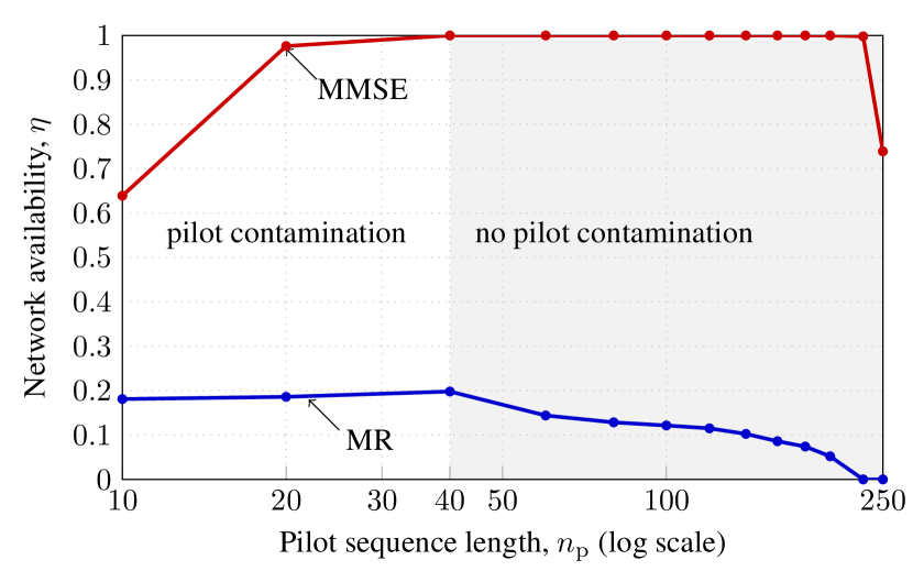
(a) Uplink transmission.

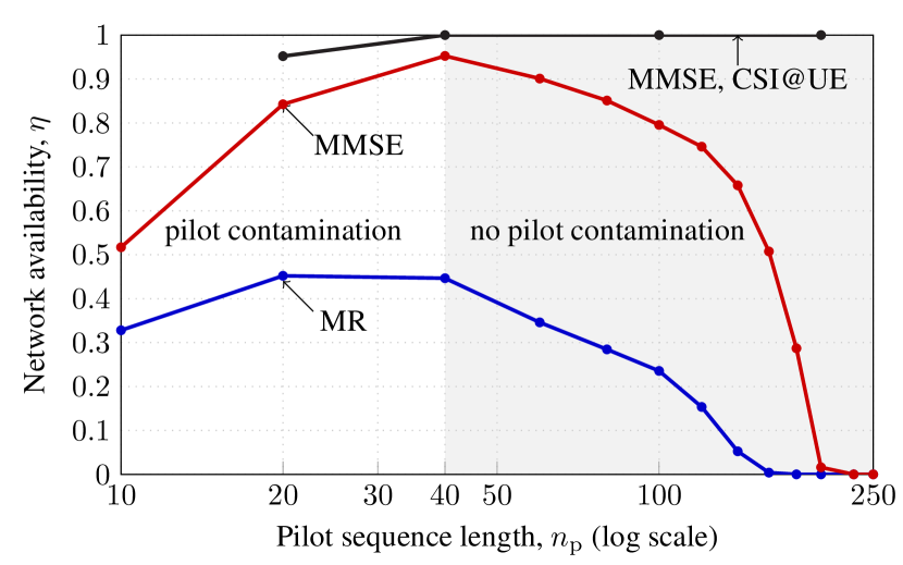
(b) Downlink transmission.

Figure 5: Network availability for $\epsilon_{\text{{}target}}=10^{-5}$. Here, $L=4$, $K=10$, $\Delta=25^{\circ}$, the cell size is $75\times 75$ m, $\rho^{\mathrm{ul}}=\rho^{\mathrm{dl}}=10\,\mathrm{dBm}$, $M=100$, $b=160$, and $n=300$.

In Fig. 5, we plot the network availability (40) for a fixed $\epsilon_{\text{{}target}}=10^{-5}$ (which is in agreement with the URLLC requirements) versus the number of pilot symbols $n_{\text{{}p}}=fK$, where we recall that $f$ is the pilot reuse factor. The results presented in Fig. 3 suggest that pilot contamination should be avoided and that MMSE should be preferred to MR. The results presented in Fig. 5 confirm these design guidelines. With multicell MMSE, a network availability above $90\%$ can be achieved in UL and DL by setting a pilot reuse factor $f=4$ such that $n_{\text{{}p}}=fK=40$. This is the minimum value of $n_{\text{{}p}}$ that results in no pilot contamination in a network with $L=4$ cells. Increasing $n_{\text{{}p}}$ further has a deleterious effect on the network availability, especially in the DL. Indeed, the corresponding reduction in the number of channel uses $n_{\text{{}dl}}=(300-n_{\text{{}p}})/2$ available for data transmission in the DL overcomes the benefits of a more accurate CSI. As already discussed, the difference in performance between UL and DL with multicell MMSE processing is due to the assumption that the UE has no CSI and performs mismatched decoding by relying on channel hardening. Indeed, when the UEs are provided with perfect CSI (black curve), the network availability achievable in UL and DL is the same. If needed, additional network-availability gains can be achieved by, e.g., increasing the number of BS antennas, by reducing the number of UEs that are served simultaneously, or by using scheduling to avoid serving at the same time UEs that are difficult to separate spatially via linear precoding. For example, in the scenario considered in Fig. 5(b), a network availability above $98\%$ can be achieved by halving the number of scheduled UEs. Finally, note that the network availability achievable with MR is below $50\%$ even when pilot contamination is avoided. This implies that in practical scenarios, MR is too sensitive to interference to achieve the low error probability targets required in URLLC.

V Conclusions

We presented guidelines on the design of Massive MIMO systems supporting the transmission of short information packets under the high reliability targets demanded in URLLC. Specifically, we showed that, for a BS equipped with up to $100$ antennas, it is imperative to avoid pilot contamination and to use MMSE spatial processing in place of the computationally less intensive MR spatial processing. Our guidelines were based on a firm nonasymptotic bound on the error probability, which is based on recent results in finite-blocklength information theory, and applies to a realistic Massive MIMO network, with imperfect channel state information, pilot contamination, spatially correlated channels, arbitrary linear spatial processing, and randomly positioned UEs. We provided an accurate approximation for this bound, based on the saddlepoint method, which makes its evaluation computationally efficient for the low error probabilities targeted in URLLC. Finally, we showed that analyses based on performance metrics such as outage probability and normal approximation, although appealing because of the simplicity of the underlying mathematical formulas, may result in a significant underestimation of the error probability, which is clearly undesirable when designing URLLC links. Results relied on the assumption that the channel covariance matrix is perfectly known to the receiver. If no such knowledge is available, the BS can perform instead least-square channel estimation followed by regularized zero forcing, at the cost of a performance loss recently quantified in [35].

Appendix A - Proof of Theorem 1

Let $\mathbf{q}=[q[1],\dots,q[n]]\sim\mathcal{CN}({\bf 0},\rho{{\bf I}_{n}})$ be the transmitted codeword and $\mathbf{v}=[v[1],\dots,v[n]]$ be the corresponding channel output obtained via the input-output relation (1). Finally, let $\bar{\mathbf{q}}=[\bar{q}[1],\dots,\bar{q}[n]]$ be a vector of i.i.d. $\mathcal{CN}(0,\rho)$ random variables, independent of both $\mathbf{q}$ and $\mathbf{v}$. Intuitively, $\bar{\mathbf{q}}$ stands for any codeword different from the transmitted one.

A simple generalization of the random coding union bound in [18, Th. 16] to the mismatched SNN decoder (2) results in the following bound

$$\epsilon\leq\operatorname{\mathbb{E}}\mathopen{}\left[\min\mathopen{}\left\{1,(m-1)f(\mathbf{q},\mathbf{v})\right\}\right]$$ (46)

where $f(\mathbf{q},\mathbf{v})=\Pr\{\lVert\mathbf{v}-\widehat{g}\bar{\mathbf{q}}\rVert^{2}\leq\lVert\mathbf{v}-\widehat{g}{\mathbf{q}}\rVert^{2}|\mathbf{q},\mathbf{v}\}$. The bound (46) is obtained by observing that, when the mismatched SNN decoder (2) is used, an error occurs if, after being scaled by $\widehat{g}$, the codeword $\bar{\mathbf{q}}$ is closer in Euclidean distance to $\mathbf{v}$ than $\mathbf{q}$, and then by using a tightened version of the union bound. We next apply the Chernoff bound to $f(\mathbf{q},\mathbf{v})$ and obtain that

$$f(\mathbf{q},\mathbf{v}) \leq \frac{\operatorname{\mathbb{E}}_{\bar{\mathbf{q}}}\mathopen{}\left[\exp\mathopen{}\left({-s\lVert\mathbf{v}-\widehat{g}\bar{\mathbf{q}}\rVert^{2}}\right)\right]}{\exp\mathopen{}\left({-s\lVert\mathbf{v}-\widehat{g}\mathbf{q}\rVert^{2}}\right)}$$ (47)

for $s>0$. Substituting (47) into (46), we conclude that

$$\epsilon \leq \mathbb{E}\Biggl{[}\min\Biggl{\{}1,\exp\Biggl{(}\log(m-1)$$ (49)

$$\qquad\qquad{}+\log\frac{\operatorname{\mathbb{E}}_{\bar{\mathbf{q}}}\mathopen{}\left[\exp\mathopen{}\left({-s\lVert\mathbf{v}-\widehat{g}\bar{\mathbf{q}}\rVert^{2}}\right)\right]}{\exp\mathopen{}\left({-s\lVert\mathbf{v}-\widehat{g}\mathbf{q}\rVert^{2}}\right)}\Biggr{)}\Biggr{\}}\Biggr{]}$$

$$= \mathbb{E}\Biggl{[}\min\Biggl{\{}1,\exp\Biggl{(}\log(m-1)$$

$$\,\,\,{}-\sum_{k=1}^{n}\log\frac{\exp\mathopen{}\left({-s|v[k]-\widehat{g}q[k]|^{2}}\right)}{\operatorname{\mathbb{E}}_{\bar{q}[k]}\mathopen{}\left[\exp\mathopen{}\left({-s|v[k]-\widehat{g}\bar{q}[k]|^{2}}\right)\right]}\Biggr{)}\Biggr{\}}\Biggr{]}.$$

Let now the generalized information density be defined as

$$\imath_{s}(q[k],v[k])=\log\frac{\exp\mathopen{}\left({-s|v[k]-\widehat{g}q[k]|^{2}}\right)}{\operatorname{\mathbb{E}}_{\bar{q}[k]}\mathopen{}\left[\exp\mathopen{}\left({-s|v[k]-\widehat{g}\bar{q}[k]|^{2}}\right)\right]}.$$ (50)

Using (50), we can rewrite (49) as

$$\epsilon \leq \mathbb{E}\Biggl{[}\min\Biggl{\{}1,\exp\Biggl{(}\log(m-1)$$ (51)

$$\qquad\qquad\qquad\quad{}-\sum_{k=1}^{n}\imath_{s}(q[k],v[k])\Biggr{)}\Biggr{\}}\Biggr{]}.$$

The desired bound (3) follows by observing that, for every positive random variable $w$, we have that $\operatorname{\mathbb{E}}\mathopen{}\left[\min\mathopen{}\left\{{1,w}\right\}\right]=\mathbb{P}\mathopen{}\left[{w\geq u}\right]$ where $u$ is uniformly distributed on $\mathopen{}\left[{0,1}\right]$.

To conclude the proof, it remains to show that the generalized information density defined in (50) can be expressed as in (4). Since $\bar{q}[k]\sim\mathcal{CN}(0,\rho)$, it follows that, for a given $v[k]$

$$|v[k]-\widehat{g}\bar{q}[k]|^{2} \stackrel{{\scriptstyle d}}{{=}} \frac{|\widehat{g}|^{2}\rho}{2}\mathopen{}\left({\mathopen{}\left({\frac{|v[k]|\sqrt{2}}{|\widehat{g}|\sqrt{\rho}}+u_{1}}\right)^{2}+u_{2}^{2}}\right)$$ (52)

$$\stackrel{{\scriptstyle d}}{{=}} \frac{|\widehat{g}|^{2}\rho}{2}\theta$$

where $u_{1}$ and $u_{2}$ are independent $\mathcal{N}(0,1)$ random variables and $\theta$ follows a noncentral chi-squared distribution with $2$ degrees of freedom and noncentrality parameter $\lambda={2|v[k]|^{2}}/(\rho|\widehat{g}|^{2})$. The MGF of $\theta$ is given by

$$\operatorname{\mathbb{E}}\mathopen{}\left[e^{\zeta\theta}\right]=\frac{\exp\mathopen{}\left({\frac{\lambda\zeta}{1-2\zeta}}\right)}{(1-2\zeta)},\quad\zeta<\frac{1}{2}.$$ (53)

Using (53) in (50) with $\zeta=-s|\widehat{g}|^{2}\rho/2$, we conclude that (50) coincides with (4).

Appendix B - Proof of (10) and (11)

In this appendix, we prove that (9) holds for every $\zeta\in[\underline{\zeta},\overline{\zeta}]$, where $\underline{\zeta}$ and $\overline{\zeta}$ are given in (10) and (11), respectively. Let $q\sim\mathcal{CN}(0,\rho)$ and $v=gq+z$ where $z\sim\mathcal{CN}(0,\sigma^{2})$, so that $v\sim\mathcal{CN}(0,\sigma_{v}^{2})$ with $\sigma_{v}^{2}=\rho\lvert g\rvert^{2}+\sigma^{2}$ Furthermore, set $A=s\lvert v-\widehat{g}q\rvert^{2}$ and $B=\gamma\lvert v\rvert^{2}$ with $\gamma=s/(1+s\rho\lvert\widehat{g}\rvert^{2})$. We can then rewrite the information density (4) as

$$\imath_{s}\mathopen{}\left({q,v}\right) = B-A+\log\mathopen{}\left({1+s\rho\lvert\widehat{g}\rvert^{2}}\right)$$ (54)

It then follows that $A$ and $B$ are dependent exponentially-distributed random variables with rate parameter $1/\beta_{A}$ defined in (12) and $1/\beta_{B}$ defined in (13), respectively. This implies that the random variable $\imath_{s}\mathopen{}\left({q,v}\right)$ involves the difference between two dependent exponentially-distributed random variables. Let $\Delta=B-A$. The probability density function (PDF) of $\Delta$ is [36, Cor. 8]

$$f_{\Delta}(\delta) = \frac{1}{\sqrt{(\beta_{B}-\beta_{A})^{2}+4\beta_{A}\beta_{B}(1-\nu)}}$$ (55)

$$\>\times\exp\mathopen{}\left({-\frac{\lvert\delta\rvert\sqrt{(\beta_{B}-\beta_{A})^{2}+4\beta_{A}\beta_{B}(1-\nu)}}{2\beta_{A}\beta_{B}(1-\nu)}}\right)$$

$$\>\times\exp\mathopen{}\left({\frac{\delta\mathopen{}\left({\beta_{B}-\beta_{A}}\right)}{2\beta_{A}\beta_{B}(1-\nu)}}\right)$$

where $\nu=\text{Cov}\mathopen{}\left({A,B}\right)/\sqrt{\text{Var}\mathopen{}\left({A}\right)\text{Var}\mathopen{}\left({B}\right)}$ is the correlation coefficient between $A$ and $B$. Using (55), we can express the MGF of $-\imath_{s}\mathopen{}\left({q,v}\right)$ as follows:

$$\!\!\!\operatorname{\mathbb{E}}\mathopen{}\left[e^{-\zeta\imath_{s}\mathopen{}\left({q,v}\right)}\right] = \frac{1}{(1+s\rho\lvert\widehat{g}\rvert^{2})^{\zeta}}\int_{-\infty}^{\infty}\exp\mathopen{}\left({-\zeta\delta}\right)f_{\Delta}(\delta)\mathrm{d}\delta$$ (56)

$$= \frac{(1+s\rho\lvert\widehat{g}\rvert^{2})^{-\zeta}}{1+(\beta_{B}-\beta_{A})\zeta-\beta_{A}\beta_{B}(1-\nu)\zeta^{2}}$$

where the last step holds for all $\zeta\in(\underline{\zeta},\overline{\zeta})$, with $\underline{\zeta}$ and $\overline{\zeta}$ given in (10) and (11), respectively. The desired result in (9) follows because the right-hand side of (56) is infinitely differentiable.

To conclude the proof, we need to show that $\nu$ in (55) is given by (14). By definition, $\text{Cov}\mathopen{}\left({A,B}\right)=\operatorname{\mathbb{E}}\mathopen{}\left[AB\right]-\operatorname{\mathbb{E}}\mathopen{}\left[A\right]\operatorname{\mathbb{E}}\mathopen{}\left[B\right]$ where

$$\operatorname{\mathbb{E}}\mathopen{}\left[AB\right]=s\gamma\operatorname{\mathbb{E}}\mathopen{}\left[\lvert v-\widehat{g}q\rvert^{2}\lvert v\rvert^{2}\right].$$ (57)

To compute this correlation, it turns out convenient to set $x=v-\widehat{g}q$ and to express $x$ as the MMSE estimate of $v$ given $x$ plus the uncorrelated estimation error $e$:

$$x=\alpha v+e.$$ (58)

Here, $\alpha$ is the MMSE coefficient, given by $\alpha=\operatorname{\mathbb{E}}\mathopen{}\left[v^{*}x\right]/\sigma_{v}^{2}$, and $e\sim\mathcal{CN}(0,\sigma_{e}^{2})$ where $\sigma_{e}^{2}=\sigma^{2}_{x}-\lvert\operatorname{\mathbb{E}}\mathopen{}\left[v^{*}x\right]\rvert^{2}/\sigma_{v}^{2}$, with $\sigma^{2}_{x}=\operatorname{\mathbb{E}}\mathopen{}\left[\lvert x\rvert^{2}\right]=\lvert g-\widehat{g}\rvert^{2}\rho+\sigma^{2}$. Note that since $e$ is Gaussian and uncorrelated with $v$, then $e$ and $v$ are independent. Using (58), we can rewrite the expectation on the right-hand side of (57) as follows:

$$\operatorname{\mathbb{E}}\mathopen{}\left[\lvert v-\widehat{g}q\rvert^{2}\lvert v\rvert^{2}\right] = \operatorname{\mathbb{E}}\mathopen{}\left[\lvert x\rvert^{2}\lvert v\rvert^{2}\right]$$ (59)

$$= \operatorname{\mathbb{E}}\mathopen{}\left[\lvert\alpha v+e\rvert^{2}\lvert v\rvert^{2}\right]$$

$$= \lvert\alpha\rvert^{2}\operatorname{\mathbb{E}}\mathopen{}\left[\lvert v\rvert^{4}\right]+\operatorname{\mathbb{E}}\mathopen{}\left[\lvert v\rvert^{2}\right]\operatorname{\mathbb{E}}\mathopen{}\left[\lvert e\rvert^{2}\right]$$

$$= 2\lvert\alpha\rvert^{2}\sigma_{v}^{4}+\sigma_{v}^{2}\sigma_{e}^{2}$$

$$= \lvert\operatorname{\mathbb{E}}\mathopen{}\left[v^{*}x\right]\rvert^{2}+\sigma_{v}^{2}\sigma_{x}^{2}.$$ (60)

Here, in (59) we used that $\operatorname{\mathbb{E}}\mathopen{}\left[\lvert v\rvert^{4}\right]=2\sigma_{v}^{4}$. Furthermore, (60) follows by the definition of $\alpha$ and of $\sigma^{2}_{e}$. Note now that $\beta_{A}=s\sigma_{x}^{2}$ and $\beta_{B}=\gamma\sigma^{2}_{v}$. Recall also that $\operatorname{\mathbb{E}}\mathopen{}\left[A\right]=\beta_{A}$, $\text{Var}\mathopen{}\left({A}\right)=\beta_{A}^{2}$, $\operatorname{\mathbb{E}}\mathopen{}\left[B\right]=\beta_{B}$, $\text{Var}\mathopen{}\left({B}\right)=\beta_{B}^{2}$. Hence, we conclude that

$$\nu=\frac{s\gamma(\lvert\operatorname{\mathbb{E}}\mathopen{}\left[v^{*}x\right]\rvert^{2}+\sigma_{v}^{2}\sigma_{x}^{2})-\beta_{A}\beta_{B}}{\beta_{A}\beta_{B}}=\frac{s\gamma\lvert\operatorname{\mathbb{E}}\mathopen{}\left[v^{*}x\right]\rvert^{2}}{\beta_{A}\beta_{B}}.$$ (61)

To obtain (14), we use that $\gamma=s/(1+s\rho\lvert\widehat{g}\rvert^{2})$ and that $\operatorname{\mathbb{E}}\mathopen{}\left[v^{*}x\right]=\sigma_{v}^{2}-g^{*}\widehat{g}\rho$.

Appendix C - Proof of Theorem 3

Substituting ${\bf u}_{1}^{\rm{MR}}=\frac{1}{M}\widehat{\mathbf{h}}_{1}$ into (31), we obtain

$$y_{1}^{\mathrm{ul}}[k]=\frac{1}{M}\widehat{\mathbf{h}}^{\mathsf{H}}_{1}\mathbf{h}_{1}x_{1}^{\mathrm{ul}}[k]+\frac{1}{M}\widehat{\mathbf{h}}^{\mathsf{H}}_{1}\mathbf{h}_{2}x_{2}^{\mathrm{ul}}[k]+\frac{1}{M}\widehat{\mathbf{h}}^{\mathsf{H}}_{1}\mathbf{z}^{\mathrm{ul}}[k].$$ (62)

Under Assumption 1 and using [6, Lem. 3], we have that, in the limit ${M\to\infty}$,

$$\frac{1}{M}\widehat{\mathbf{h}}^{\mathsf{H}}_{1}\mathbf{h}_{1}\mathop{\asymp}^{(a)}\frac{1}{M}\widehat{\mathbf{h}}^{\mathsf{H}}_{1}{\widehat{\mathbf{h}}}_{1}\asymp\frac{1}{M}\mathrm{tr}({\bf{\Phi}}_{1})\,\text{and}\,\frac{1}{M}\widehat{\mathbf{h}}^{\mathsf{H}}_{1}\mathbf{z}^{\mathrm{ul}}[k]\mathop{\asymp}^{(b)}0.$$ (63)

Here, ${(a)}$ and $(b)$ follow because ${\widehat{\mathbf{h}}}_{1}$ and the pair $({\widetilde{\mathbf{h}}}_{1},\mathbf{z}^{\mathrm{ul}}[k])$ are independent. Similarly, we have that

$$\frac{1}{M}\widehat{\mathbf{h}}^{\mathsf{H}}_{1}\mathbf{h}_{2} \asymp 0,\text{ if }\bm{\phi}_{1}\neq\bm{\phi}_{2}\;\text{with}\;\bm{\phi}_{1}^{\mbox{\tiny$\mathrm{H}$}}\bm{\phi}_{2}=0,$$ (64)

$$\frac{1}{M}\widehat{\mathbf{h}}^{\mathsf{H}}_{1}\mathbf{h}_{2} \asymp \frac{1}{M}\widehat{\mathbf{h}}^{\mathsf{H}}_{1}{\widehat{\mathbf{h}}}_{2}\mathop{\asymp}^{(c)}\frac{1}{M}\mathrm{tr}({\bf\Upsilon}_{12}),\text{ if }\bm{\phi}_{1}=\bm{\phi}_{2}$$ (65)

where ${(c)}$ follows from the fact that ${\widehat{\mathbf{h}}}_{1}$ and ${\widehat{\mathbf{h}}}_{2}$ are correlated under pilot contamination. Using (63), (64), and (65) in (62), we conclude that

$$\!\!\!y_{1}^{\mathrm{ul}}[k] \asymp \frac{1}{M}\mathrm{tr}({\bf{\Phi}}_{1})x_{1}^{\mathrm{ul}}[k],\text{ if }\bm{\phi}_{1}\neq\bm{\phi}_{2}\;\text{with}\;\bm{\phi}_{1}^{\mbox{\tiny$\mathrm{H}$}}\bm{\phi}_{2}=0,\!\!$$

$$\!\!\!y_{1}^{\mathrm{ul}}[k] \asymp \frac{\mathrm{tr}({\bf{\Phi}}_{1})x_{1}^{\mathrm{ul}}[k]+\mathrm{tr}({\bf\Upsilon}_{12})x_{2}^{\mathrm{ul}}[k]}{M},\text{ if }\bm{\phi}_{1}=\bm{\phi}_{2}.\!\!$$ (67)

This implies that, in the absence of pilot contamination, the input-output relation becomes that of a deterministic noiseless channel as $M\to\infty$, while it converges to that of an AWGN channel with transmit power $\lim_{M\to\infty}[\frac{1}{M}\mathrm{tr}({\bf{\Phi}}_{1})]^{2}$ and noise variance $\lim_{M\to\infty}[\frac{1}{M}\mathrm{tr}({\bf\Upsilon}_{12})]^{2}$ when the two UEs use the same pilot sequence. Note also that $g\asymp\widehat{g}\asymp\frac{1}{M}\mathrm{tr}({\bf{\Phi}}_{1})$ where $g$ and $\widehat{g}$ are defined in (33). The desired result then follows from (6).

Appendix D - Proof of Theorem 4

We only consider the case in which the two UEs use the same pilot sequence, i.e., $\bm{\phi}_{1}=\bm{\phi}_{2}$. By applying the matrix inversion lemma (see, e.g., [6, Lem. 4]) we can rewrite (34) as

$${\bf u}_{1}^{\rm{MMSE}} = \left(\sum\limits_{i=1}^{2}\widehat{\mathbf{h}}_{i}\widehat{\mathbf{h}}_{i}^{\mbox{\tiny$\mathrm{H}$}}+{\bf Z}\right)^{-1}\widehat{\mathbf{h}}_{1}$$ (68)

$$= \frac{1}{1+\gamma_{1}^{\text{ul}}}\left(\widehat{\mathbf{h}}_{2}\widehat{\mathbf{h}}_{2}^{\mbox{\tiny$\mathrm{H}$}}+{\bf Z}\right)^{-1}\widehat{\mathbf{h}}_{1}$$ (69)

where we have set $\gamma_{1}^{\text{ul}}=\widehat{\mathbf{h}}_{1}^{\mathsf{H}}\left(\widehat{\mathbf{h}}_{2}\widehat{\mathbf{h}}_{2}^{\mathsf{H}}+{\bf Z}\right)^{-1}\widehat{\mathbf{h}}_{1}$. Substituting (69) into (31) we obtain, after multiplying and dividing each term by $M$,

$$y_{1}^{\text{ul}} = \frac{1}{\frac{1}{M}+\frac{\gamma_{1}^{\text{ul}}}{M}}\frac{1}{M}\widehat{\mathbf{h}}_{1}^{\mathsf{H}}\left(\widehat{\mathbf{h}}_{2}\widehat{\mathbf{h}}_{2}^{\mathsf{H}}+{\bf Z}\right)^{-1}\!\!\!\mathbf{h}_{1}x_{1}^{\text{ul}}$$ (70)

$${}+\frac{1}{\frac{1}{M}+\frac{\gamma_{1}^{\text{ul}}}{M}}\frac{1}{M}\widehat{\mathbf{h}}_{1}^{\mathsf{H}}\left(\widehat{\mathbf{h}}_{2}\widehat{\mathbf{h}}_{2}^{\mathsf{H}}+{\bf Z}\right)^{-1}\!\!\!\mathbf{h}_{2}x_{2}^{\text{ul}}$$

$${}+\frac{1}{\frac{1}{M}+\frac{\gamma_{1}^{\text{ul}}}{M}}\frac{1}{M}\widehat{\mathbf{h}}_{1}^{\mathsf{H}}\left(\widehat{\mathbf{h}}_{2}\widehat{\mathbf{h}}_{2}^{\mathsf{H}}+{\bf Z}\right)^{-1}\!\!\!\mathbf{z}^{\text{ul}}.$$

We begin by considering the first term. Under Assumption 1 and using [6, Lem. 3], we obtain

$$\frac{1}{M}\widehat{\mathbf{h}}_{1}^{\mathsf{H}}\left(\widehat{\mathbf{h}}_{2}\widehat{\mathbf{h}}_{2}^{\mathsf{H}}+{\bf Z}\right)^{-1}\!\!\!\mathbf{h}_{1}\asymp\frac{\gamma_{1}^{\text{ul}}}{M}$$ (71)

since $\mathbf{h}_{1}=\widehat{\mathbf{h}}_{1}+\widetilde{\mathbf{h}}_{1}$ with $\widetilde{\mathbf{h}}_{1}$ being independent from $\widehat{\mathbf{h}}_{1}$ and $\widehat{\mathbf{h}}_{2}$. We note that, under Assumptions 1 and 2, $\frac{\gamma_{1}^{\text{ul}}}{M}$ converges to a finite value as $M\to\infty$ [6, App. B]. This ensures that

$$\frac{\frac{\gamma_{1}^{\text{ul}}}{M}}{\frac{1}{M}+\frac{\gamma_{1}^{\text{ul}}}{M}}x_{1}^{\text{ul}}\asymp x_{1}^{\text{ul}}.$$ (72)

By applying [6, Lem. 5] to the second term in (70), we obtain

$$\IEEEeqnarraymulticol{3}{l}{\frac{1}{\frac{1}{M}+\frac{\gamma_{1}^{\text{ul}}}{M}}\frac{1}{M}\widehat{\mathbf{h}}_{1}^{\mathsf{H}}\left(\widehat{\mathbf{h}}_{2}\widehat{\mathbf{h}}_{2}^{\mathsf{H}}+{\bf Z}\right)^{-1}{\mathbf{h}}_{2}}$$

$$= \frac{1}{\frac{1}{M}+\frac{\gamma_{1}^{\text{ul}}}{M}}\Biggl{(}\frac{1}{M}\widehat{\mathbf{h}}_{1}^{\mathsf{H}}{\bf Z}^{-1}{\mathbf{h}}_{2}$$ (73)

$$\qquad\qquad\qquad{}-\frac{\frac{1}{M}\widehat{\mathbf{h}}_{1}^{\mathsf{H}}{\bf Z}^{-1}\widehat{\mathbf{h}}_{2}\frac{1}{M}\widehat{\mathbf{h}}_{2}^{\mathsf{H}}{\bf Z}^{-1}{\mathbf{h}}_{2}}{\frac{1}{M}+\frac{1}{M}\widehat{\mathbf{h}}_{2}^{\mathsf{H}}{\bf Z}^{-1}{\widehat{\mathbf{h}}_{2}}}\Biggr{)}.$$

Under Assumption 1 and using [6, Lem. 3], we have that, as ${M\to\infty}$,

$$\frac{1}{M}\widehat{\bf h}_{1}^{\mbox{\tiny$\mathrm{H}$}}{\bf Z}^{-1}{\bf h}_{2} \asymp\frac{1}{M}\widehat{\bf h}_{1}^{\mbox{\tiny$\mathrm{H}$}}{\bf Z}^{-1}\widehat{\bf h}_{2}\asymp\frac{1}{M}\mathrm{tr}({\bf\Upsilon}_{12}{\bf Z}^{-1})\triangleq\beta_{12}$$ (74)

$$\frac{1}{M}\widehat{\bf h}_{2}^{\mbox{\tiny$\mathrm{H}$}}{\bf Z}^{-1}\widehat{\bf h}_{2} \asymp\frac{1}{M}\mathrm{tr}({\bf\Phi}_{2}{\bf Z}^{-1})\triangleq\beta_{22}.$$ (75)

Substituting (74) and (75) in (73) and using Assumption 2, we conclude that

$$\frac{\frac{1}{M}}{\frac{1}{M}+\frac{\gamma_{1}^{\text{ul}}}{M}}\widehat{\mathbf{h}}_{1}^{\mathsf{H}}\left(\widehat{\mathbf{h}}_{2}\widehat{\mathbf{h}}_{2}^{\mathsf{H}}+{\bf Z}\right)^{-1}{\mathbf{h}}_{2} \asymp \frac{M}{\gamma_{1}^{\text{ul}}}\left(\beta_{12}-\frac{\beta_{12}\beta_{22}}{\beta_{22}}\right)$$ (76)

$$= 0$$

since $\frac{\gamma_{1}^{\text{ul}}}{M}$ converges to a finite value as $M\to\infty$ [6, App. B]. For the third term in (70), we have

$$\IEEEeqnarraymulticol{3}{l}{\frac{1}{\frac{1}{M}+\frac{\gamma_{1}^{\text{ul}}}{M}}\frac{1}{M}\widehat{\mathbf{h}}_{1}^{\mathsf{H}}\left(\widehat{\mathbf{h}}_{2}\widehat{\mathbf{h}}_{2}^{\mathsf{H}}+{\bf Z}\right)^{-1}\!\!\!\mathbf{z}^{\text{ul}}}$$

$$= \frac{1}{\frac{1}{M}+\frac{\gamma_{1}^{\text{ul}}}{M}}\Biggl{(}\frac{1}{M}\widehat{\mathbf{h}}_{1}^{\mathsf{H}}{\bf Z}^{-1}\mathbf{z}^{\text{ul}}$$ (77)

$$\qquad\qquad\qquad{}-\frac{\frac{1}{M}\widehat{\mathbf{h}}_{1}^{\mathsf{H}}{\bf Z}^{-1}\widehat{\mathbf{h}}_{2}^{\mathsf{H}}\frac{1}{M}\widehat{\mathbf{h}}_{2}^{\mathsf{H}}{\bf Z}^{-1}\mathbf{z}^{\text{ul}}}{\frac{1}{M}+\frac{1}{M}\widehat{\mathbf{h}}_{2}^{\mathsf{H}}{\bf Z}^{-1}{\widehat{\mathbf{h}}_{2}}}\Biggr{)}.$$

Under Assumption 1 and using [6, Lem. 3], we have that, as ${M\to\infty}$,

$$\frac{1}{M}\widehat{\mathbf{h}}_{1}^{\mathsf{H}}{\bf Z}^{-1}\mathbf{z}^{\text{ul}}\asymp 0\quad\text{and}\quad\frac{1}{M}\widehat{\mathbf{h}}_{2}^{\mathsf{H}}{\bf Z}^{-1}\mathbf{z}^{\text{ul}}\asymp 0$$ (78)

where we have used that $({\widehat{\mathbf{h}}_{1}},{\widehat{\mathbf{h}}_{2}})$ and $\mathbf{z}^{\text{ul}}$ are independent. Therefore, we have that

$$\frac{1}{\frac{1}{M}+\frac{\gamma_{1}^{\text{ul}}}{M}}\frac{1}{M}\widehat{\mathbf{h}}_{1}^{\mathsf{H}}\left(\widehat{\mathbf{h}}_{2}\widehat{\mathbf{h}}_{2}^{\mathsf{H}}+{\bf Z}\right)^{-1}\mathbf{z}^{\text{ul}}\asymp 0.$$ (79)

Combining all the above results, we conclude that $y_{1}^{\text{ul}}\asymp x_{1}^{\text{ul}}$. This implies that, as $M\to\infty$, the input-output relation (70) converges to that of a deterministic noiseless channel. The desired result then follows from (6).

References

• [1] J. Östman, A. Lancho, and G. Durisi, “Short-packet transmission over a bidirectional massive MIMO link,” in Proc. Asilomar Conf. Signals, Syst., Comput., Pacific Grove, CA, USA, Dec. 2019.
• [2] 3GPP, “NR; NR and NG-RAN Overall description; Stage-2,” 3rd Generation Partnership Project (3GPP), Technical Specification (TS), 9 2019, version 15.7.0.
• [3] ——, “Service requirements for cyber-physical control applications in vertical domains,” 3rd Generation Partnership Project (3GPP), Technical Specification (TS) 22.104, 12 2019, version 17.2.0.
• [4] T. L. Marzetta, “Noncooperative cellular wireless with unlimited numbers of base station antennas,” IEEE Trans. Wireless Commun., vol. 9, no. 11, pp. 3590–3600, Nov. 2010.
• [5] H. Q. Ngo, E. G. Larsson, and T. L. Marzetta, “Energy and spectral efficiency of very large multiuser MIMO systems,” IEEE Trans. Commun., vol. 61, no. 4, pp. 1436–1449, Apr. 2013.
• [6] E. Björnson, J. Hoydis, and L. Sanguinetti, “Massive MIMO has unlimited capacity,” IEEE Trans. Wireless Commun., vol. 17, no. 1, pp. 574–590, Jan. 2018.
• [7] E. Björnson, L. Sanguinetti, J. Hoydis, and M. Debbah, “Optimal design of energy-efficient multi-user MIMO systems: Is Massive MIMO the answer?” IEEE Trans. Wireless Commun., vol. 14, no. 6, pp. 3059–3075, Jun. 2015.
• [8] H. V. Cheng, E. Björnson, and E. G. Larsson, “Optimal pilot and payload power control in single-cell massive MIMO systems,” IEEE Trans. Signal Process., vol. 65, no. 9, pp. 2363–2378, May 2017.
• [9] E. Björnson, L. Sanguinetti, H. Wymeersch, J. Hoydis, and T. L. Marzetta, “Massive MIMO is a reality—what is next?: Five promising research directions for antenna arrays,” Digital Signal Processing, vol. 94, pp. 3–20, Nov. 2019.
• [10] G. Durisi, T. Koch, and P. Popovski, “Towards massive, ultra-reliable, and low-latency wireless communication with short packets,” Proc. IEEE, vol. 104, no. 9, pp. 1711–1726, Sep. 2016.
• [11] E. Björnson, J. Hoydis, and L. Sanguinetti, “Massive MIMO networks: Spectral, energy, and hardware efficiency,” Foundations and Trends® in Signal Processing, vol. 11, no. 3-4, pp. 154–655, Nov. 2017.
• [12] T. L. Marzetta, E. G. Larsson, H. Yang, and H. Q. Ngo, Fundamentals of massive MIMO.   London, U.K.: Cambridge Univ. Press, 2016.
• [13] M. Karlsson, E. Björnsson, and E. G. Larsson, “Performance of in-band transmission of system information in massive MIMO systems,” IEEE Trans. Wireless Commun., vol. 17, no. 3, pp. 1700–1712, Mar. 2018.
• [14] A. Bana, G. Xu, E. D. Carvalho, and P. Popovski, “Ultra reliable low latency communications in massive multi-antenna systems,” in Proc. Asilomar Conf. Signals, Syst., Comput., Pacific Grove, CA, USA, Oct. 2018, pp. 188–192.
• [15] L. H. Ozarow, S. Shamai (Shitz), and A. D. Wyner, “Information theoretic considerations for cellular mobile radio,” IEEE Trans. Veh. Technol., vol. 43, no. 2, pp. 359–378, May 1994.
• [16] W. Yang, G. Durisi, T. Koch, and Y. Polyanskiy, “Quasi-static multiple-antenna fading channels at finite blocklength,” IEEE Trans. Inf. Theory, vol. 60, no. 7, pp. 4232–4265, Jul. 2014.
• [17] A. Lapidoth and S. Shamai (Shitz), “Fading channels: How perfect need ‘perfect side information’ be?” IEEE Trans. Inf. Theory, vol. 48, no. 5, pp. 1118–1134, May 2002.
• [18] Y. Polyanskiy, H. V. Poor, and S. Verdú, “Channel coding rate in the finite blocklength regime,” IEEE Trans. Inf. Theory, vol. 56, no. 5, pp. 2307–2359, May 2010.
• [19] G. Durisi, T. Koch, J. Östman, Y. Polyanskiy, and W. Yang, “Short-packet communications over multiple-antenna Rayleigh-fading channels,” IEEE Trans. Commun., vol. 64, no. 2, pp. 618–629, Feb. 2016.
• [20] J. Östman, G. Durisi, E. G. Ström, M. C. Coskun, and G. Liva, “Short packets over block-memoryless fading channels: Pilot-assisted or noncoherent transmission?” IEEE Trans. Commun., vol. 67, no. 2, pp. 1521–1536, Feb. 2019.
• [21] J. Zeng, T. Lv, R. P. Liu, X. Su, Y. J. Guo, and N. C. Beaulieu, “Enabling ultra-reliable and low-latency communications under shadow fading by massive MU-MIMO,” IEEE Internet of Things J., vol. 7, no. 1, pp. 234–246, Jan. 2020.
• [22] H. Ren, C. Pan, Y. Deng, M. Elkashlan, and A. Nallanathan, “Joint pilot and payload power allocation for massive-MIMO-enabled URLLC IIoT networks,” IEEE J. Sel. Areas Commun., vol. 38, no. 5, pp. 816–830, May 2020.
• [23] A. Martinez and A. Guillén i Fàbregas, “Saddlepoint approximation of random–coding bounds,” in Proc. Inf. Theory Applicat. Workshop (ITA), San Diego, CA, USA, Feb. 2011.
• [24] W. Feller, An Introduction to Probability Theory and Its Applications, 2nd ed., New York, NY, USA, 1971, vol. II.
• [25] A. Lancho, J. Östman, G. Durisi, T. Koch, and G. Vazquez-Vilar, “Saddlepoint approximations for short-packet wireless communications,” IEEE Trans. Wireless Commun., vol. 19, no. 7, pp. 4831–4846, Jul. 2020.
• [26] L. Sanguinetti, E. Björnsson, and J. Hoydis, “Towards massive MIMO 2.0: Understanding spatial correlation, interference suppression, and pilot contamination,” IEEE Trans. Commun., vol. 68, no. 1, pp. 232–257, Jan. 2020.
• [27] M. Haenggi, “The meta distribution of the SIR in Poisson bipolar and cellular networks,” IEEE Trans. Wireless Commun., vol. 15, no. 4, pp. 2577–2589, Apr. 2016.
• [28] R. G. Gallager, Information Theory and Reliable Communication.   New York, NY, U.S.A.: John Wiley & Sons, 1968.
• [29] E. MolavianJazi, “A unified approach to Gaussian channels with finite blocklength,” Ph.D. dissertation, University of Notre Dame, Notre Dame, IN, 2014.
• [30] E. Biglieri, J. G. Proakis, and S. Shamai (Shitz), “Fading channels: Information-theoretic and communications aspects,” IEEE Trans. Inf. Theory, vol. 44, no. 6, pp. 2619–2692, Oct. 1998.
• [31] J. Scarlett, A. Martinez, and A. Guillén i Fàbregas, “Mismatched decoding: Error exponents, second-order rates and saddlepoint approximations,” IEEE Trans. Inf. Theory, vol. 60, no. 5, pp. 2647–2666, May 2014.
• [32] G. Kaplan and S. Shamai, “Information rates and error exponents of compound channels with application to antipodal signaling in a fading environment,” Arch. Elek. Über, vol. 47, no. 4, pp. 228–239, 1993.
• [33] E. Björnson, L. Sanguinetti, and M. Debbah, “Massive MIMO with imperfect channel covariance information,” in 2016 50th Asilomar Conference on Signals, Systems and Computers, 2016, pp. 974–978.
• [34] J. Hoydis, S. ten Brink, and M. Debbah, “Massive MIMO in the UL/DL of cellular networks: How many antennas do we need?” IEEE J. Sel. Areas Commun., vol. 31, no. 2, pp. 574–590, Feb. 2013.
• [35] A. Lancho, J. Östman, G. Durisi, and L. Sanguinetti, “A finite-blocklength analysis for URLLC with massive MIMO,” in Proc. IEEE Int. Conf. Commun. (ICC), Montreal, Canada, Jun. 2021.
• [36] H. Holm and M.-S. Alouini, “Sum and difference of two squared correlated Nakagami variates in connection with the McKay distribution,” IEEE Trans. Commun., vol. 52, no. 8, pp. 1367–1376, Aug. 2004.