On the distribution of lattice points on hyperbolic circles

Abstract.

We study the fine distribution of lattice points lying on expanding circles in the hyperbolic plane $\mathbb{H}$. The angles of lattice points arising from the orbit of the modular group ${\hbox{PSL}_{2}({\mathbb{Z}})}$, and lying on hyperbolic circles, are shown to be equidistributed for generic radii. However, the angles fail to equidistribute on a thin set of exceptional radii, even in the presence of growing multiplicity. Surprisingly, the distribution of angles on hyperbolic circles turns out to be related to the angular distribution of $\mathbb{Z}^{2}$-lattice points (with certain parity conditions) lying on circles in $\mathbb{R}^{2}$, along a thin subsequence of radii. A notable difference is that measures in the hyperbolic setting can break symmetry — on very thin subsequences they are not invariant under rotation by $\frac{\pi}{2}$, unlike the Euclidean setting where all measures have this invariance property.

1. Introduction

1.1. Background and motivation

We study the angular distribution of lattice points on hyperbolic circles — the boundary of balls with respect to the hyperbolic distance — and show that equidistribution holds “generically” as the radius grows. We also show that there are subsequences where equidistribution fails to hold, even if the multiplicity is growing. Refined equidistribution results of this style have been studied for the case of Euclidean circles in [29]. For the case of the $n$-dimensional hyperbolic space $\mathbb{H}^{n}$ equidistribution results for large annuli of fixed width were studied in [1, 15, 31, 38, 40, 43].

In this paper we focus on the $2$-dimensional case. Let $\mathbb{H}:=\mathbb{H}^{2}$ denote the hyperbolic plane which can be identified with the upper half plane

$$\mathbb{H}=\left\{x+iy:x\in\mathbb{R},y\in\mathbb{R}_{>0}\right\}.$$

The plane $\mathbb{H}$ is equipped with the hyperbolic distance $\rho(\cdot,\cdot)$, that for $z,w\in\mathbb{H}$ is given by the relation

(1.1) $$\cosh(\rho(z,w))=1+\frac{|z-w|^{2}}{2\Im(z)\Im(w)}.$$

The projective special linear group ${\hbox{PSL}_{2}({\mathbb{R}})}:={\hbox{SL}_{2}({\mathbb{R}})}/\{\pm I\}$ acts on $\mathbb{H}$ by Möbius transformations: for

$$\gamma=\begin{pmatrix}a&b\\ c&d\end{pmatrix}\in{\hbox{PSL}_{2}({\mathbb{R}})}$$

and $z\in\mathbb{H}$ fixed, the standard action is given by

$$\gamma(z)=\frac{az+b}{cz+d}.$$

In fact, ${\hbox{PSL}_{2}({\mathbb{R}})}$ is precisely the group of orientation preserving isometries of $\mathbb{H}$.

We will consider discrete subsets of $\mathbb{H}$ given by the orbit of various subsets of the modular group $\Gamma={\hbox{PSL}_{2}({\mathbb{Z}})}$. (The case of congruence subgroups introduces some interesting novel features, and will be addressed in future work). With $w=i$ and $z=\gamma(i)$ we have

(1.2) $$2\cosh(\rho(\gamma(i),i))=\|\gamma\|^{2}=a^{2}+b^{2}+c^{2}+d^{2}.$$

For $n\in{\mathbb{N}}$ let $\Gamma^{n}:=\{\gamma\in\Gamma:\|\gamma\|^{2}=n\}$, and define the set

(1.3) $$\mathcal{N}:=\{n\in\mathbb{N}:|\Gamma^{n}|>0\}=\left\{n=a^{2}+b^{2}+c^{2}+d^{2}\in\mathbb{N}:\begin{pmatrix}a&b\\ c&d\end{pmatrix}\in\Gamma\right\}.$$

We wish to determine the distribution of the points $\{\gamma(i):\gamma\in\Gamma^{n}\}$ as $n$ grows along integers $n\in\mathcal{N}$. It is convenient to conformally map $\mathbb{H}$ into the hyperbolic disc $\mathbb{D}=\{z\in\mathbb{C},|z|<1\}$ (endowed with the hyperbolic metric) by

(1.4) $$f(z)=\frac{z-i}{1-iz}.$$

Clearly $f(i)=0$, and the points $f(\gamma(i))$, for $\gamma\in\Gamma^{n}$ all lie on a circle centered at $0$. Thus, to determine the distribution of lattice points on the original hyperbolic circle it suffices to determine the distribution of angles (or complex arguments)

$$\theta(\gamma):=\arg f(\gamma(i))$$

as $\gamma$ ranges over elements in $\Gamma^{n}$. In order to study the set of possible configurations we define probability measures $\mu_{n}$ (for $n\in\mathcal{N}$) on $S^{1}$, supported on a finite number of points, by letting

(1.5) $$\mu_{n}:=\frac{1}{|\Gamma^{n}|}\sum_{\gamma\in\Gamma^{n}}\delta_{\theta(\gamma)}.$$

1.2. Statement of the principal results

1.2.1. Generic equidistribution

Our first result states that lattice points arising from the action of the modular group are asymptotically equidistributed for “generic” $n\in\mathcal{N}$, in the sense that $\mu_{n}$ weakly tends to $\mu_{\text{Haar}}$ for $n$ tending to infinity along a generic subsequence, where $\mu_{\text{Haar}}$ denotes the Haar measure on $S^{1}$ normalized to have mass one. (For an illustration of approximate equidistribution, we plot two example point configurations in Figure 1). In fact, stronger than that, we give a quantitative bound for the discrepancy.

Theorem 1.1.

Letting $\mathcal{N}(x)=\{n\in\mathcal{N}:n\leq x\}$ we have $\mathcal{N}(x)\asymp x/\log x$. Further, for all but $o(|\mathcal{N}(x)|)$ integers $n\in\mathcal{N}(x)$, we have $|\Gamma^{n}|\asymp(\log n)^{\log 2\pm o(1)}$ and moreover

$$\sup_{I\subset S^{1}}\left|\frac{|\{\gamma\in\Gamma^{n}:\theta(\gamma)\in I\}|}{|\Gamma^{n}|}-\frac{|I|}{2\pi}\right|\ll\frac{1}{|\Gamma^{n}|^{\vartheta-o(1)}},$$

where $\vartheta=\log(\pi/2)/\log 2=0.651496129\ldots$.

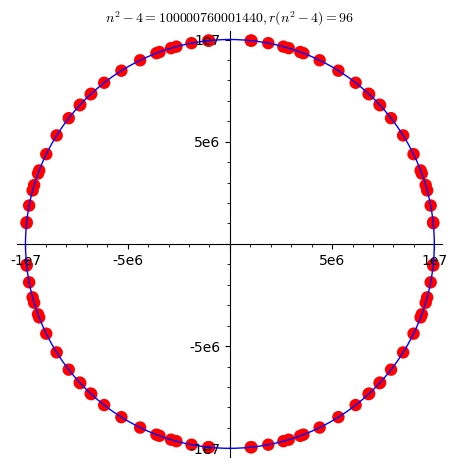
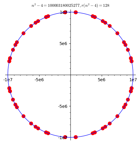
Figure 1. Left: Points $(x,y)\in{\mathbb{Z}}^{2}$ s.t. $x^{2}+y^{2}=n^{2}-4$. Right: Points $(x,y)\in{\mathbb{Z}}^{2}$ s.t. $x^{2}+y^{2}=n^{2}-4$ and $x$ even.

As a corollary to Theorem 1.1, we determine the distribution, for generic $n\in{\mathcal{N}}$ tending to infinity, of the real parts $\{\Re\gamma(i)\,(\operatorname{mod}1):\gamma\in\Gamma^{n}\},$ and show (cf. Section 6) that the corresponding probability density function is given by

(1.6) $$p(x)=\frac{1}{\pi}\sum_{k\in{\mathbb{Z}}}\frac{1}{1+(x+k)^{2}}=\frac{\cosh(\pi)\cdot\sinh(\pi)}{\cosh(\pi)^{2}-\cos(\pi x)^{2}},\quad x\in[0,1].$$

That is, for an interval $I\subseteq[0,1]$, the proportion of those $\gamma\in\Gamma^{n}$ with $\Re\gamma(i)\,(\operatorname{mod}1)\in I$ is asymptotically given by $\int_{I}p(x)dx$ as $n\rightarrow\infty$ along a density one subsequence of $n\in\mathcal{N}$. This can be viewed as a thin set analogue of the equidistribution result attributed to Good for the set $\{\Re\gamma(z)\,(\operatorname{mod}1):\gamma\in{\hbox{PSL}_{2}({\mathbb{Z}})},\Im\gamma(z)\geq\varepsilon\}$, as $\varepsilon\to 0$ (see [35, Theorem 6.2], [16, Eq. (3.27)] and [38, Theorem 1.2]). However, while real parts modulo one are equidistributed when ordering by the imaginary part (in particular having constant probability density functions), ordering by distance to $i$ introduces minute fluctuations, cf. Figure 2.

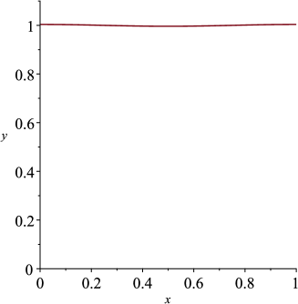
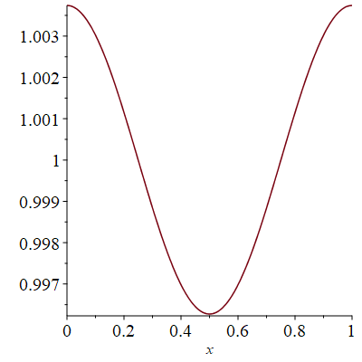
Figure 2. Left: The plot of the asymptotic probability density function $p(x)=\frac{\cosh(\pi)\cdot\sinh(\pi)}{\cosh(\pi)^{2}-\cos(\pi x)^{2}}$ of $\{\Re\gamma(i)\,(\operatorname{mod}1):\gamma\in\Gamma^{n}\}$ along a generic sequence $\{n\}\subseteq{\mathcal{N}}$. Right: Same plot, magnified in the $y$-direction.

A key ingredient in the proof of Theorem 1.1 is the remarkable fact that the set of hyperbolic angles $\{\theta(\gamma):\gamma\in\Gamma^{n}\}$ is the same as the set of angles of Euclidean ${\mathbb{Z}}^{2}$-lattice points, having even $x$-coordinate, on the circle of radius $\sqrt{n^{2}-4}$. (In essence, integer points on the surface given by the two equations $a^{2}+b^{2}+c^{2}+d^{2}=n$ and $ad-bc=1$ can be identified with integer points on the curve given by $4x^{2}+y^{2}=n^{2}-4$.)

Proposition 1.2.

Let ${\mathcal{S}}:=\{x^{2}+y^{2}:\>x,y\in{\mathbb{Z}}\}$ denote the set of integers expressible as sums of two integer squares. Then $\mathcal{N}=\{n\in{\mathbb{Z}}:n^{2}-4\in\mathcal{S}\}$ and, for $n\in\mathcal{N}$, we have

(1.7) $$\{\theta(\gamma):\gamma\in\Gamma^{n}\}=\left\{\arg(x+iy):x,y\in{\mathbb{Z}},x\equiv 0\,(\operatorname{mod}2),x^{2}+y^{2}=n^{2}-4\right\}.$$

1.2.2. Non-equidistribution

We can also show that there are subsequences $n_{i}\in\mathcal{N}$ tending to infinity in such a way that $|\Gamma^{n_{i}}|\to\infty$, yet the angles $\{\theta(\gamma):\gamma\in\Gamma^{n_{i}}\}$ fail to equidistribute. The constraint $|\Gamma^{n_{i}}|\to\infty$ is natural, since equidistribution clearly fails along sequences so that $|\Gamma^{n_{i}}|$ stays bounded (such sequences do exist, see e.g. [28, Proposition 2.1]).

We will construct a wide family of weak-$*$ partial limits of the sequence $\{\mu_{n}\}_{n\in\mathcal{N}}$ of probability measures on $S^{1}$, by comparing the hyperbolic setting to its Euclidean analogue, i.e. the case of the angular distribution of the points of ${\mathbb{Z}}^{2}\subseteq{\mathbb{R}}^{2}$. To describe the setup we need some further notation. Given $n\in{\mathbb{Z}}$, let

$$r(n):=|\{(x,y)\in{\mathbb{Z}}^{2}:x^{2}+y^{2}=n\}|$$

denote the number of representations of $n$ as sum of two squares, and given $n\in{\mathcal{S}}$, define a probability measure $\nu_{n}$ on $S^{1}$ by

(1.8) $$\nu_{n}:=\frac{1}{r(n)}\sum_{(x,y)\in{\mathbb{Z}}^{2}:x^{2}+y^{2}=n}\delta_{\arg(x+iy)},$$

supported precisely on the angles corresponding to these representations.

We say that a probability measure on $S^{1}$ is attainable from lattice points on circles, or simply just attainable, (cf. [29, Definition 1.1]) if it is a weak-$*$ partial limit of $\{\nu_{n}\}_{n\in{\mathcal{S}}}$. Our second principal result asserts that every attainable measure, under a small perturbation, is a weak-$*$ partial limit of $\{\mu_{n}\}_{n\in{\mathcal{N}}}$ in (1.5).

Theorem 1.3.

There exists an absolute constant $C>0$, so that for every probability measure $\nu$ on $S^{1}$ that is attainable, there exists a sequence $\{n_{i}\}\subseteq\mathcal{N}$ and a probability measure $\widetilde{\nu}$ supported on at most $C$ points on $S^{1}$, such that

$$\mu_{n_{i}}\Rightarrow\nu\star\tilde{\nu}.$$

Whether or not $\nu$ is supported on a finite number of points, we may impose the further condition that $|\Gamma^{n_{i}}|$ grows as $n_{i}\rightarrow\infty$.

In particular there exists a sequence $\{n_{i}\}\subseteq\mathcal{N}$ such that $|\Gamma^{n_{i}}|\to\infty$, and the weak-$*$ limit $\mu=\lim_{i\to\infty}\mu_{n_{i}}$ is highly singular in the sense of having support on a finite number of points, see Figure 3 for illustration.

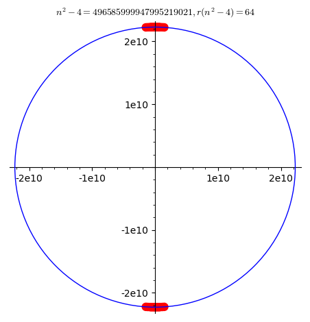
Figure 3. Points $(x,y)\in{\mathbb{Z}}^{2}$ s.t. $x^{2}+y^{2}=n^{2}-4$ and $x$ even.

Further, there are hyperbolic limiting measures $\mu=\nu\star\tilde{\nu}$ that are singular continuous — for example, we may take $\nu$ to be a measure of Cantor type with arbitrary small support (cf. [29, §4.3]).

1.2.3. Breaking symmetry

We remark that for $n\equiv 0\,(\operatorname{mod}4)$ the parity condition on the $x$-coordinate in (1.7) is illusory: both $x$ and $y$ must be even if $x^{2}+y^{2}=n^{2}-4\equiv 0\,(\operatorname{mod}4)$, and in this case the angles are obtained from all lattice points on the circle of radius $\sqrt{n^{2}-4}$. In particular, any measure (1.5) (or any weak-$*$ limit along even $n\in\mathcal{N}$) must be invariant under $(x,y)\to(x,-y)$ as well as rotation by $\frac{\pi}{2}$.

However, for $n$ odd, the parity condition breaks the quarter rotation symmetry, yet the limiting measures along “generic” odd $n$’s are equidistributed by Theorem 1.1 — hence invariant under all rotations. A natural question is whether or not there exist limit measures of $\mu_{n}$, along subsequences $n_{i}$ so that $|\Gamma^{n_{i}}|$ tends to infinity, that are not invariant under rotation by $\frac{\pi}{2}$. This is indeed the case.

Theorem 1.4.

There exists weak-$*$ limit points of $\{\mu_{n}\}_{n\in\mathcal{N}}$, along subsequences so that $|\Gamma^{n}|$ tends to infinity, which are asymmetric in the sense of not being invariant under rotation by $\frac{\pi}{2}$. In particular, the weak-$*$ limit points of $\{\mu_{n}\}_{n\in\mathcal{N}}$ do not coincide with those of $\{\nu_{n}\}_{n\in{\mathcal{S}}}$.

1.3. Comparison with the Euclidean case

It is natural to compare our results with those for the case of lattice points of $\mathbb{Z}^{2}$ inside $\mathbb{R}^{2}$. In that case, a more precise description of the (aforementioned “attainable”) limit measures can be given; in fact, a partial classification of the first two nontrivial Fourier coefficients of the limit measures was done by Kurlberg and Wigman [29], and Sartori  [41], building upon the pioneering works of Cilleruelo [6], Katai-Környei [25] and Erdős-Hall [9]; our discrepancy bound can be viewed as a thin subset analog, of comparable strength, to the discrepancy bounds in [9, 25]. In the Euclidean setting the set of limit measures turns out to have a surprising ‘fractal structure’; an analogous statement for the orbit points of the modular group would follow from plausible conjectures related to twin primes in arithmetic progressions.

1.4. Discussion on hyperbolic lattice point counting

The study of the orbit under the action of Fuchsian groups on the hyperbolic plane with the use of spectral theory goes back to Delsarte [7] (also see [8, pp. 829-845]), Huber [21], Selberg [42] (with the best error term), and Patterson [37]. Nicholls [36], using ergodic theory, worked out the case of the $n$-dimensional space, and Günther [17], using spectral theory, generalized Selberg’s result for the case of rank one spaces. Refined results in the hyperbolic lattice point problem have been extensively studied, such as the angle distribution [1, 15, 31, 38, 40, 43] and the pair correlation density [2, 3, 31, 26, 39]. Second moment estimates of the error term and their applications to the study of quadratic forms and correlation sums of $r(n)$ were addressed by Chamizo [4, 5] and Iwaniec [23]. Further, Friedlander and Iwaniec [11] studied a modified ‘hyperbolic’ prime number theorem. Although coming from a different problem, their work is more ‘arithmetic’ in flavor rather than spectral, and it is closer to our own approach.

Our investigation was inspired by the results of Marklof and Vinogradov [31], who resolved the local statistics of lattice points lying on spherical shells of fixed width, projected on the unit sphere, including the correlation functions of arbitrary order, finer than their angular equidistribution due to Nicholls [36]. Namely, for $\gamma\in\Gamma$ and a fixed point $w\in\mathbb{H}$, denote by $\phi(\gamma w)=\phi_{i}(\gamma w)$ the intersection of the unit hyperbolic circle centered at $i\in\mathbb{H}$ and the semi-infinite geodesic starting at $i$ and containing $\gamma w$. Fix $s\geq 0$, and, for $t>s$ large, consider the projection

$$\mathcal{P}_{w}(s,t)=\{\phi(\gamma w):\gamma\in\Gamma/\Gamma_{w},\,t-s\leq\rho(\gamma w,i)<t\}$$

of the emerging spherical shell to the unit circle. Here $\Gamma_{w}$ is the stabilizer of the point $w\in\mathbb{H}$, which is a finite cyclic group [23, Ch. 2]. These notions easily extend to the case of a lattice $\Gamma$ acting discontinuously on the $n$-dimensional hyperbolic space $\mathbb{H}^{n}$ for $n\geq 2$.

In this context the main research line has been on understanding the direction distribution in $\mathcal{P}_{w}(s,t)$ as $t\rightarrow\infty$, with $s$ fixed. By work of Nicholls [36], asymptotics for the counting function is known:

$$\left|\mathcal{P}_{w}(s,t)\right|\sim c_{n}\left(1-e^{-(n-1)s}\right)\cdot e^{(n-1)t},$$

for $t\to\infty$ and $s$ fixed (here $c_{n}$ is an explicit constant depending on $n$ and $\Gamma$). Further, by  [36, Theorem 2] it easily follows that the angles in $\mathcal{P}_{w}(s,t)$ asymptotically equidistribute: for every $\mathcal{A}\subset\mathbb{S}^{n-1}$ with measure zero boundary and $s$ fixed we have

$$\left|\mathcal{P}_{w}(s,t)\cap\mathcal{A}\right|\sim\frac{\operatorname*{vol}(\mathcal{A})}{\operatorname*{vol}(\mathbb{S}^{n-1})}\cdot\left|\mathcal{P}_{w}(s,t)\right|$$

as $t\to\infty$.

Our method differs from the usual attacks on hyperbolic lattice counting problem. The equivalence between hyperbolic angular distribution and Euclidean angular distribution allows us to use arithmetic tools (sieves) rather than results from spectral or ergodic theory.

1.5. Acknowledgments

D.C. was supported by the Labex CEMPI (ANR-11-LABX-0007-01) and is currently supported by an IdEx postdoctoral fellowship at IBM, University of Bordeaux. P.K. was partially supported by the Swedish Research Council (2016-03701). S.L. is partially supported by EPSRC Standard Grant EP/T028343/1. The research leading to these results has received funding from the European Research Council under the European Union’s Seventh Framework Programme (FP7/2007-2013), ERC grant agreement n${}^{\text{o}}$ 335141 (D.C. and I.W.). We would like to thank D. R. Heath-Brown and J. Marklof for discussions that inspired the research presented in this manuscript, and Z. Rudnick for comments on an earlier version of this manuscript and a very helpful discussion regarding A. Good’s results.

2. Lattice points in $\mathbb{H}$ and ${\mathbb{R}}^{2}$: proof of Proposition 1.2

2.1. Lattice points on hyperbolic and Euclidean circles

For $\gamma=\left(\begin{smallmatrix}a&b\\ c&d\end{smallmatrix}\right)\in\Gamma$ and $i\in\{1,2,3,4\}$, define the quadratic forms $x_{i}=x_{i}(\gamma)$ by

(2.1) $$x_{1}=a^{2}+b^{2},\quad x_{2}=c^{2}+d^{2},\quad x_{3}=ac+bd,\quad x_{4}=x_{1}-x_{2};$$

we then find that $\gamma(i)=(x_{3}+i)/x_{2}\in\mathbb{H}$, and, using that $x_{3}^{2}=x_{1}x_{2}-1$, a short calculation gives

$$f(\gamma(i))=\frac{2x_{3}+ix_{4}}{x_{1}+x_{2}+2}\in\mathbb{D}.$$

Thus, with $n=\|\gamma\|^{2}=a^{2}+b^{2}+c^{2}+d^{2}\in{\mathbb{N}}$, the set of hyperbolic angles is given by the angles (in ${\mathbb{R}}^{2}$) of the set of points

$$L_{n}:=\left\{(2(ac+bd),a^{2}+b^{2}-c^{2}-d^{2}):a^{2}+b^{2}+c^{2}+d^{2}=n,\begin{pmatrix}a&b\\ c&d\end{pmatrix}\in\Gamma\right\}.$$

We observe that the set $L=\bigcup\limits_{n=1}^{\infty}L_{n}$ is not a sublattice of $\mathbb{Z}^{2}$, and, in what follows, we will show that $L_{n}$ can be identified with the set

$$\mathcal{L}_{n}=\left\{(2x_{3},x_{4}):x_{3},x_{4}\in{\mathbb{Z}},4x_{3}^{2}+x_{4}^{2}=n^{2}-4\right\}.$$

To describe this identification in more detail, let $a,b,c,d\in{\mathbb{Z}}$ satisfy

$$a^{2}+b^{2}+c^{2}+d^{2}=n,\quad ad-bc=1.$$

Then, following [11] or [12, Chapter 14.7] (see also [23, Ch.12] and [4]), we let

(2.2) $$y_{1}=a+d,\quad y_{2}=b-c,\quad y_{3}=b+c,\quad y_{4}=a-d.$$

It is then simple to verify that

$$y_{1}^{2}+y_{2}^{2}=a^{2}+b^{2}+c^{2}+d^{2}+2(ad-bc)=n+2$$

and

$$y_{3}^{2}+y_{4}^{2}=a^{2}+b^{2}+c^{2}+d^{2}-2(ad-bc)=n-2,$$

indicating a correspondence between hyperbolic lattice points, and Euclidean lattice points on two circles. With $\mathcal{N}$ defined as in (1.3), and recalling that $\mathcal{S}=\{n\in\mathbb{Z}:r(n)>0\}$, the above demonstrates that $\mathcal{N}\subseteq\{n\in{\mathbb{Z}}:n\pm 2\in\mathcal{S}\}$.

2.2. The parity conditions

Conversely, we will now show that $\{n\in{\mathbb{Z}}:n\pm 2\in\mathcal{S}\}\subseteq\mathcal{N}$. This gives rise to certain parity conditions that must be taken into account.

First, note that if $n\in\{n\in{\mathbb{Z}}:n\pm 2\in\mathcal{S}\}$ then $n+2\not\equiv 3\,(\operatorname{mod}4)$ (recall that $k\not\in\mathcal{S}$ for any $k\equiv 3\,(\operatorname{mod}4)$). Also, if $n+2\equiv 2\,(\operatorname{mod}4)$, write $n=4m$; as $n+2=2(2m+1)$ and $n-2=2(2m-1)$ we find that $n+2\not\in\mathcal{S}$ or $n-2\not\in\mathcal{S}$. It remains to consider integers $n$ with $n+2\equiv 0,1\,(\operatorname{mod}4)$. Let $y_{1},y_{2},y_{3},y_{4}\in\mathbb{Z}$ satisfy

(2.3) $$y_{1}^{2}+y_{2}^{2}=n+2\qquad\text{ and }\qquad y_{3}^{2}+y_{4}^{2}=n-2.$$

Define

(2.4) $$a=(y_{1}+y_{4})/2,\quad b=(y_{2}+y_{3})/2,\quad c=(y_{3}-y_{2})/2,\quad d=(y_{1}-y_{4})/2.$$

Clearly, $a^{2}+b^{2}+c^{2}+d^{2}=n$ and $ad-bc=1$. We also need that $a,b,c,d\in\mathbb{Z}$, i.e., that $y_{1}\equiv y_{4}\,(\operatorname{mod}2)$, and $y_{2}\equiv y_{3}\,(\operatorname{mod}2)$.

To analyze the implications, consider first the case $n+2\equiv n-2\equiv 0\,(\operatorname{mod}4)$. We find that, by (2.3), $y_{1},y_{2},y_{3},y_{4}$ all must be even, and the parity condition is satisfied automatically.

Otherwise, consider the case $n+2\equiv n-2\equiv 1\,(\operatorname{mod}4)$. By using (2.3) again, we find that $y_{1},y_{2}$ must be of opposite parity, and the same holds for $y_{3},y_{4}$. The parity conditions $y_{1}\equiv y_{4}\,(\operatorname{mod}2)$ and $y_{2}\equiv y_{3}\,(\operatorname{mod}2)$ are now nontrivial, and, by symmetry, only half the solutions on the two circles yield hyperbolic lattice points. The parity condition can be ensured, if necessary, by interchanging $y_{1}$ and $y_{2}$.

2.3. Proof of Proposition 1.2

We next relate the distribution of hyperbolic angles to the distribution of angles of Euclidean lattice points, with even $x$-coordinates, on one circle.

Proof.

We first show $L_{n}\subseteq\mathcal{L}_{n}$. Let $y_{1},\ldots,y_{4}$ be as in (2.2). We find that

$$(y_{1}+iy_{2})(y_{3}+iy_{4}) = y_{1}y_{3}-y_{2}y_{4}+i(y_{1}y_{4}+y_{2}y_{3})$$

$$= (a+d)(b+c)-(b-c)(a-d)$$

$$+i((a+d)(a-d)+(b-c)(b+c))$$

$$= 2(ac+bd)+i(a^{2}+b^{2}-c^{2}-d^{2})$$

$$= 2x_{3}+ix_{4}$$

with $x_{3},x_{4}$ as in (2.1); it is straightforward to check that $2x_{3}^{2}+x_{4}^{2}=n^{2}-4$, so $L_{n}\subseteq\mathcal{L}_{n}$.

Let $(2u,v)\in\mathbb{Z}^{2}$ with $4u^{2}+v^{2}=n^{2}-4$. Since $(n-2,n+2)|4$, we have that $n^{2}-4\in\mathcal{S}$ if and only if $n\pm 2\in\mathcal{S}$. It follows that there exist integers $y_{1},y_{2},y_{3},y_{4}$ with

$$y_{1}^{2}+y_{2}^{2}=n-2,\qquad y_{3}^{2}+y_{4}^{2}=n+2,$$

and $(y_{1}+iy_{2})(y_{3}+iy_{4})=2u+iv$. In particular, $y_{1}y_{3}-y_{2}y_{4}$ must be even. Recall from Section 2.2 that we only need to consider $n+2\equiv n-2\equiv 0,1\,(\operatorname{mod}4)$. Hence, since $y_{1}y_{3}-y_{2}y_{4}$ is even, the parity conditions $y_{1}\equiv y_{4}\,(\operatorname{mod}2)$ and $y_{2}\equiv y_{3}\,(\operatorname{mod}2)$ hold (interchanging $y_{1}$ and $y_{2}$ if needed). Thus, for $a,b,c,d$ as in (2.4) we have that $a^{2}+b^{2}+c^{2}+d^{2}=n$, $ad-bc=1$ and $a,b,c,d\in\mathbb{Z}$. By repeating the calculation performed in (2.3) we have $2u=2(ac+bd)$ and $v=a^{2}+b^{2}-c^{2}-d^{2}$. Therefore, $\mathcal{L}_{n}\subseteq L_{n}$.

∎

3. Equidistribution discrepancy estimate: Proof of Theorem 1.1

3.1. Auxiliary notation

For $\vec{x}\in\mathbb{R}^{2}$ let $\theta(\vec{x})$ denote the angle between $\vec{x}$ and the positive $x$-axis. Also, let $1_{S}$ denote the indicator function of a set $S$. We also write

$$\omega_{1}(n)=|\{p|n:p\equiv 1\,(\operatorname{mod}4)\}|,\quad\text{ and }\quad\Omega_{1}(n)=\sum_{\begin{subarray}{c}p^{a}||n\\ p\equiv 1\,(\operatorname{mod}4)\end{subarray}}a,$$

where $p^{a}||n$, means $p^{a}|n$ and $p^{a+1}\nmid n$. Further, let

(3.1) $$r^{\star}(n)=\sum_{\begin{subarray}{c}\vec{x}=(x,y)\in\mathbb{Z}^{2}\\ |\vec{x}|^{2}=n\\ x\text{ is even}\end{subarray}}1.$$

If $n$ is odd then $r^{\star}(n)=\tfrac{1}{2}r(n)$ since for every $\vec{x}=(x,y)$ with $|\vec{x}|^{2}=n$ either $x$ or $y$ is even, so by symmetry exactly one-half of the lattice points on the circle of radius $\sqrt{n}$ will have even $x$-coordinate. Next, consider $n=2m$ with $m$ odd then $r^{\star}(n)=0$ since for $|\vec{x}|^{2}=2m$ there exists $a,b\in\mathbb{Z}$ with $x+iy=(1+i)(a+ib)=(a-b)+i(b+a)$ and either $a$ or $b$ is even ($m$ is odd) so $x$ and $y$ are both odd. Finally, if $n=4m$ and $x^{2}+y^{2}=4m$, then $x+iy=2(a+ib)$ for some $a,b\in\mathbb{Z}$, so $x,y$ are even and in this case $r^{\star}(n)=r(n)$. In summary,

(3.2) $$r^{\star}(n)=\begin{cases}\tfrac{1}{2}\cdot r(n)&\text{ if }n\equiv\pm 1\!\!\!\!\pmod{4},\\ 0&\text{ if }n\equiv 2\!\!\!\!\pmod{4},\\ r(n)&\text{ if }n\equiv 0\!\!\!\!\pmod{4}.\end{cases}$$

Additionally, let

$$\tau_{\ell}(n)=\sum_{n_{1}\cdots n_{\ell}=n}1$$

denote the $\ell$-fold divisor function, and define $b(n)=1$ if $n$ is a sum of two squares and to be equal to zero otherwise (i.e. $b(\cdot)$ is the characteristic function of $\mathcal{S}=\{n=\square+\square\}$).

Definition 3.1 (Primary numbers).

A Gaussian integer $a+ib\in\mathbb{Z}[i]$ is primary if $a+ib\equiv 1\,(\operatorname{mod}{2(1+i)})$. Equivalently, $a+ib$ is primary if

$$\begin{split}b\equiv&0\,(\operatorname{mod}2)\\ a\equiv&1-b\,(\operatorname{mod}4).\end{split}$$

It is well-known that a product of two primary Gaussian integers is primary, and each primary Gaussian integer can be factored uniquely, up to reordering, into primary Gaussian primes, see e.g. [24, p. 54]. For a prime $p\equiv 1\,(\operatorname{mod}4)$, let $\pi$ be the primary Gaussian prime with norm $N\pi=p$ and $\Im(\pi)>0$. We define

(3.3) $$\theta_{p}=\operatorname{Arg}(\pi)$$

where $\operatorname{Arg}(\cdot)$ is the principal value of the argument function.

3.2. Proof of Theorem 1.1

By Proposition 1.2, Theorem 1.1 is an immediate consequence of the following discrepancy bound for integral lattice points, having even $x$-coordinate, on circles with radii $\sqrt{n^{2}-4}$.

Proposition 3.2.

Along a density one subsequence of integers $n$ such that $n^{2}-4$ is a sum of two squares we have that $r^{\star}(n^{2}-4)\asymp(\log n)^{\log 2\pm o(1)}$ and moreover

(3.4) $$\sup\limits_{I\subseteq S^{1}}\bigg{|}\frac{1}{r^{\star}(n^{2}-4)}\sum_{\begin{subarray}{c}\vec{x}=(x,y)\in\mathbb{Z}^{2}\\ |\vec{x}|^{2}=n^{2}-4\\ x\text{ is even}\end{subarray}}1_{I}(\theta(\vec{x}))-\frac{|I|}{2\pi}\bigg{|}\ll\frac{1}{r^{\star}(n^{2}-4)^{\vartheta-o(1)}},$$

where $\vartheta=\log(\pi/2)/\log 2=0.651496129\ldots.$

Towards a proof of Proposition 3.2 we record the following consequence of the work of Nair-Tenenbaum [34, Eq. (7)]. Let $h\in\mathbb{Z}$ and $f,g$ be non-negative multiplicative functions such that $f(n)\leq\tau_{\ell}(n)$ and $g(n)\leq\tau_{\ell}(n)$ for some $\ell$. Then

(3.5) $$\sum_{n\leq X}f(n)g(n+h)\ll X\prod_{p\leq X}\left(1+\frac{f(p)-1}{p}\right)\left(1+\frac{g(p)-1}{p}\right)$$

where the implied constant depends on $h$ (alternatively see [12, Theorem 15.6], which would suffice for our purposes). Additionally, let us recall Hooley’s result [20, Theorem 3] that

(3.6) $$\sum_{n\leq X}b(n-2)b(n+2)\gg\frac{X}{\log X}.$$

Finally we record the following estimate, which follows from the work of Erdős-Hall [9]. Given an odd prime $p\equiv 1\,(\operatorname{mod}4)$, define

(3.7) $$\vartheta_{p}:=\arctan(y/x)$$

where $p=x^{2}+y^{2}$ with $0\leq y\leq x$, and note that $|\cos(k\theta_{p})|=|\cos(k\vartheta_{p})|$ for $k\in\mathbb{Z}$ with $2|k$. Hence, for any $k\in\mathbb{Z}$ with $2|k$ it follows from repeating the argument in [9, Eqs. (24)-(25)] that

(3.8) $$\sum_{\begin{subarray}{c}p\leq X\\ p\equiv 1\!\!\!\!\pmod{4}\end{subarray}}|\cos(k\theta_{p})|=\frac{1}{\pi}\int_{2}^{X}\frac{dt}{\log t}+O\bigg{(}|k|Xe^{-c\sqrt{\log X}}\bigg{)},$$

for some $c>0$.

Before proving Proposition 3.2 we need the following simple estimate.

Lemma 3.3.

Let $\varepsilon>0$ be fixed but sufficiently small. Then

(3.9) $$\sum_{\begin{subarray}{c}n\leq X\\ \omega_{1}(n^{2}-4)\leq(1-\varepsilon)\log\log X\end{subarray}}b(n^{2}-4)\ll\frac{X}{(\log X)^{1+\frac{1}{2}\varepsilon^{2}}}.$$

Also

(3.10) $$\sum_{\begin{subarray}{c}n\leq X\\ \Omega_{1}(n^{2}-4)\geq(1+\varepsilon)\log\log X\end{subarray}}b(n^{2}-4)\ll\frac{X}{(\log X)^{1+\frac{1}{3}\varepsilon^{2}}}.$$

Remark.

For $r^{\star}(n)\neq 0$, we have that

$$2^{\omega_{1}(n)}\leq r^{\star}(n)\leq 2^{\Omega_{1}(n)+2}.$$

Hence, by (3.9) and (3.10) we have for all integers $n\leq x$ with $r^{\star}(n^{2}-4)\neq 0$ that outside of an exceptional set of size at most $O(X/(\log X)^{1+\frac{1}{3}\varepsilon^{2}})$

(3.11) $$r^{\star}(n^{2}-4)\asymp(\log n)^{\log 2\pm 2\varepsilon}.$$

Proof.

Applying Chernoff’s bound and (3.5) we have for any $\alpha>0$

$$\begin{split}\sum_{\begin{subarray}{c}n\leq X\\ \omega_{1}(n^{2}-4)\leq(1-\varepsilon)\log\log X\end{subarray}}b(n^{2}-4)&\leq(\log X)^{(1-\varepsilon)\alpha}\sum_{\begin{subarray}{c}n\leq X\end{subarray}}b(n^{2}-4)e^{-\alpha\omega_{1}(n^{2}-4)}\\ &\ll X(\log X)^{(1-\varepsilon)\alpha}\prod_{p\leq X}\left(1+\frac{b(p)e^{-\alpha}-1}{p}\right)^{2}\\ &\ll\frac{X}{\log X}(\log X)^{\alpha(1-\varepsilon)+e^{-\alpha}-1}.\end{split}$$

Taking $\alpha=\varepsilon$ it follows that $\alpha(1-\varepsilon)+e^{-\alpha}-1\leq-\varepsilon^{2}/2,$ which completes the proof of (3.9). The proof of (3.10) follows from a similar argument, which we will omit. ∎

Proof of Proposition 3.2.

For $n$ such that $b(n)=1$, $n\not\equiv 2\,(\operatorname{mod}4)$ and $k\in\mathbb{Z}$ let

(3.12) $$\begin{split}u_{k}(n)&:=\frac{1}{r(n)}\sum_{\begin{subarray}{c}\vec{x}\in\mathbb{Z}^{2}\\ |\vec{x}|^{2}=n\end{subarray}}e^{ik\theta(\vec{x})},\qquad\qquad v_{k}(n):=\frac{1}{r^{\star}(n)}\sum_{\begin{subarray}{c}\vec{x}=(x,y)\in\mathbb{Z}^{2}\\ |\vec{x}|^{2}=n\\ x\text{ is even}\end{subarray}}e^{ik\theta(\vec{x})},\end{split}$$

and

(3.13) $$w_{k}(n):=\frac{4}{r(n)}\sum_{\begin{subarray}{c}\vec{x}=(x,y)\in\mathbb{Z}^{2}\\ |\vec{x}|^{2}=n\\ x+iy\text{ is primary}\end{subarray}}e^{ik\theta(\vec{x})}.$$

The function $w_{k}(\cdot)$ is multiplicative, and for $4|k$ we have that $u_{k}(n)$ is multiplicative (if $4\nmid k$ then $u_{k}(n)=0$). Also, for any integer $m$, if $k$ is odd then $v_{k}(m)=0$, which can be seen by noting that $\theta(-x,-y)\equiv\pi+\theta(x,y)\,(\operatorname{mod}2\pi)$; so if $k$ is odd the terms corresponding to $(x,y)$,$(-x,-y)$ in the sum cancel with one another. Let us also record the following basic property

(3.14) $$v_{k}(n)=v_{-k}(n),$$

which follows from making the change of variables $(x,y)\rightarrow(x,-y)$.

Since $x+iy$ is primary if and only if $x-iy$ is primary, by grouping together terms with their conjugates it follows that $w_{k}(n)$ is real-valued, so that

(3.15) $$w_{k}(n)=\overline{w_{k}(n)}=w_{-k}(n).$$

Below we will prove that if $n$ is odd, then

(3.16) $$v_{k}(n)=(-1)^{k/2}w_{k}(n),$$

for $2|k$. Hence, by the Erdős-Turan inequality (see [32, Corollary 1.1]) and (3.16), it follows that the l.h.s. in (3.4) is, for odd $n\leq X$, bounded by

$$\ll\frac{1}{\log X}+\sum_{\begin{subarray}{c}1\leq k\leq\log X\\ 2|k\end{subarray}}\frac{|w_{k}(n^{2}-4)|}{k}.$$

Let $\varepsilon>0$ be sufficiently small but fixed and let

$$N(X)=\left\{n\leq X:b(n^{2}-4)=1\text{ and }\omega_{1}(n^{2}-4)\geq(1-\varepsilon)\log\log X\right\},$$

$$N_{\text{odd}}(X)=\left\{n\in N(X):n\text{ is odd}\right\},$$

and $N_{\text{even}}(X)$ be defined similarly. By Lemma 3.3 and (3.6),

(3.17) $$\frac{1}{|\{n\leq X:b(n^{2}-4)=1\}|}\sum_{\begin{subarray}{c}n\leq X\\ \omega_{1}(n^{2}-4)\leq(1-\varepsilon)\log\log X\end{subarray}}b(n^{2}-4)\ll\frac{1}{(\log X)^{\frac{1}{2}\varepsilon^{2}}},$$

so, for results concerning a density one subsequence of integers with $b(n^{2}-4)=1$, it suffices to consider $n\in N(X)$.

Applying Chebyshev’s inequality we get that

(3.18) $$\begin{split}&\bigg{|}\bigg{\{}n\in N_{\text{odd}}(X):\sum_{\begin{subarray}{c}1\leq k\leq\log X\\ 2|k\end{subarray}}\frac{|w_{k}(n^{2}-4)|}{k}\geq(\log X)^{-\log\frac{\pi}{2}+\varepsilon}\bigg{\}}\bigg{|}\\ &\leq(\log X)^{\log\frac{\pi}{2}-\varepsilon}\sum_{\begin{subarray}{c}1\leq k\leq\log X\\ 2|k\end{subarray}}\frac{1}{k}\sum_{\begin{subarray}{c}n\leq X\\ \omega_{1}(n^{2}-4)\geq(1-\varepsilon)\log\log X\\ n\text{ is odd}\end{subarray}}\left|w_{k}(n^{2}-4)\right|.\end{split}$$

To bound the sum on the r.h.s. of (3.18) we apply Chernoff’s bound and (3.5) to get for any $\alpha>0$ and $1\leq k\leq\log X$ that

$$\begin{split}\sum_{\begin{subarray}{c}n\leq X\\ \omega_{1}(n^{2}-4)\geq(1-\varepsilon)\log\log X\\ n\text{ is odd}\end{subarray}}|w_{k}(n^{2}-4)|\leq&\frac{1}{(\log X)^{\alpha(1-\varepsilon)}}\sum_{\begin{subarray}{c}n\leq X\\ n\text{ is odd}\end{subarray}}|w_{k}(n+2)|e^{\alpha\omega_{1}(n+2)}\cdot|w_{k}(n-2)|e^{\alpha\omega_{1}(n-2)}\\ \ll&\frac{X}{(\log X)^{\alpha(1-\varepsilon)}}\prod_{p\leq X}\left(1+\frac{|w_{k}(p)|e^{\alpha}b(p)-1}{p}\right)^{2}.\end{split}$$

Applying (3.8), the above quantity is bounded by

$$\ll\frac{X}{\log X}(\log X)^{e^{\alpha}\frac{2}{\pi}-\alpha-1+\alpha\varepsilon},$$

and after taking $\alpha=\log\pi/2$ we get that this is $\ll\frac{X}{\log X}(\log X)^{(-1+\varepsilon)\log\pi/2}.$ Using this estimate in (3.18) along with (3.11) and (3.17) shows that the bound (3.4) holds for all odd $n\leq X$ such that $b(n^{2}-4)=1$ outside a set of size

$$\ll\frac{X(\log\log X)}{(\log X)^{1+\varepsilon-\varepsilon\log\pi/2}}+\frac{X}{(\log X)^{1+\frac{1}{3}\varepsilon^{2}}}.$$

This completes the proof of Proposition 3.2 for odd $n$.

We now show that for almost all even $n$ the discrepancy (i.e. (3.4)) is small. For even $n=2m$ we have $4|n^{2}-4$, hence $v_{k}(n^{2}-4)=u_{k}(n^{2}-4)$. Also,

$$|u_{k}(n^{2}-4)|\leq|u_{k}(m+1)\cdot u_{k}(m-1)|,$$

which follows from the multiplicativity of $u_{k}(n)$ and the observation that $|u_{k}(2^{a})|=1$ for $4|k$, which can be seen by analyzing the solutions $x,y\in\mathbb{Z}$ to $x^{2}+y^{2}=2^{a}$ (recall if $4\nmid k$ then $u_{k}(n)=0$). Hence, proceeding as before, we obtain the desired discrepancy bound for almost all even $n$ as well.

It remains to establish the claim, i.e. (3.16). To see this first note that for a function with $f(z)=f(\overline{z})$ we have

(3.19) $$\begin{split}\sum_{\begin{subarray}{c}a+ib\in\mathbb{Z}[i]\\ a\text{ is even}\\ b\text{ is odd}\end{subarray}}f(a+ib)=&\sum_{\begin{subarray}{c}a+ib\in\mathbb{Z}[i]\\ a\text{ is odd}\\ b\text{ is even}\end{subarray}}f(i(a+ib))\\ =&\sum_{\begin{subarray}{c}a+ib\in\mathbb{Z}[i]\\ a\equiv 1-b\!\!\!\!\pmod{4}\\ b\text{ is even}\end{subarray}}f(-b+ai)+\sum_{\begin{subarray}{c}a+ib\in\mathbb{Z}[i]\\ -a\equiv 1-b\!\!\!\!\pmod{4}\\ b\text{ is even}\end{subarray}}f(-b+ai)\\ =&\sum_{\begin{subarray}{c}a+ib\in\mathbb{Z}[i]\\ a\equiv 1-b\!\!\!\!\pmod{4}\\ b\text{ is even}\end{subarray}}f(-b+ai)+\sum_{\begin{subarray}{c}a+ib\in\mathbb{Z}[i]\\ a\equiv 1-b\!\!\!\!\pmod{4}\\ b\text{ is even}\end{subarray}}f(-b-ai)\\ =&2\sum_{\begin{subarray}{c}a+ib\in\mathbb{Z}[i]\\ a+ib\text{ is primary}\end{subarray}}f(i(a+ib)),\end{split}$$

provided the sums above are absolutely convergent. Taking

$$f(z)=(e^{ik\arg(z)}+e^{-ik\operatorname{arg}(z)})1_{|z|^{2}=n},$$

with $2|k$, and applying (3.2), (3.14), (3.15) and (3.19) we get that

$$2v_{k}(n)=v_{k}(n)+v_{-k}(n)=2(-1)^{k/2}(w_{k}(n)+w_{-k}(n))\frac{r(n)}{4r^{\star}(n)}=2(-1)^{k/2}w_{k}(n),$$

which establishes (3.16). ∎

4. Non-uniform limits: proof of Theorem 1.3

In this subsection we show that there exist sparse subsequences of integers $\{n_{j}\}_{j}$ such that $r^{\star}(n_{j}^{2}-4)\rightarrow\infty$ as $j\rightarrow\infty$, and the integral lattice points on circles of radii $\sqrt{n_{j}^{2}-4}$ with even $x$-coordinates fail to equidistribute as $j\rightarrow\infty$. A key ingredient (Lemma 4.1 below) is a result of Kurlberg-Lester-Rosenzweig [28], which builds on related works of Huxley-Iwaniec [22] and Friedlander-Iwaniec [12, Theorem 14.8].

We also use a construction, which exploits the fact that Gaussian primes are equidistributed in narrow sectors. This follows from work of Kubilius [27] who proved that

$$\left|\left\{p\leq X:p\equiv 1\,(\operatorname{mod}{4})\text{ and }|\vartheta_{p}|\leq X^{-1/10}\right\}\right|\gg\frac{X^{9/10}}{\log X}.$$

Using the estimate above, it follows that there exists $Q<(\log X)^{1/{10}}$ which is squarefree such that $|\{p:p|Q\}|\asymp\log\log\log X$ and if $p|Q$ then $\log\log X\leq p\leq(\log\log X)^{2}$, $p\equiv 1\,(\operatorname{mod}4)$ and $|\vartheta_{p}|\leq(\log\log X)^{-1/10}$.

Lemma 4.1.

Let $m_{0}$ be an integer such that $p|m_{0}$ implies $p\equiv 1\,(\operatorname{mod}4)$. Suppose $m_{0}=f^{2}e$ where $e$ is squarefree, $1\leq e\leq\sqrt{\log\log X}$ and $f\ll 1$. Also, let $Q$ be as above. Then there exist $\gg\frac{X}{(\log X)^{2+o(1)}}$ integers $n\leq X$ such that

$$n^{2}-4=m_{0}p_{1}p_{2}Q\ell_{n}$$

where $p_{1},p_{2}$ are distinct primes $\equiv 1\,(\operatorname{mod}4)$ with $|\vartheta_{p}|\leq(\log\log X)^{-1/2}$, $p_{1},p_{2}\geq\log X$ and $r^{\star}(\ell_{n})\asymp 1$. Additionally, $m_{0},\ell_{n},p_{1},p_{2},Q$ are pairwise co-prime.

Proof.

This follows from [28, Proposition 2.1] with $Q_{0}=1$ and $Q_{1}=m_{0}Q$ and $\varepsilon=(\log\log X)^{-1/2}$, and here $n-2=p_{1}p_{2}$ and $n+2=m_{0}Q\ell_{n}$, so $(p_{1}p_{2},\ell_{n})=1$. Note that each of the prime factors of $\ell_{n}$ are $\geq X^{\eta}$ for some small but fixed $\eta>0$ so that $(\ell_{n},Q)=(\ell_{n},m_{0})=(Q,m_{0})=1$. ∎

Proof of Theorem 1.3.

By Lemma 4.1 there exist $\gg X/(\log X)^{2+o(1)}$ integers $n\leq X$ such that $n^{2}-4=m_{0}\ell_{n}Q^{\prime}$, where $Q^{\prime}=Qp_{1}p_{2}$. Moreover $Q^{\prime},\ell_{n},m_{0}$ are pairwise co-prime. Also, for a prime $p|Q^{\prime}$ we have $\theta_{p}=l_{p}\frac{\pi}{2}+O((\log\log X)^{-1/10})$ for some $l_{p}\in\mathbb{Z}$, where $\theta_{p}$ is as defined in (3.3). Let $u_{n}=(-1)^{\sum_{p|Q^{\prime}}\ell_{p}}$ and using the fact that $w_{k}(\cdot)$ is multiplicative we have for $2|k$

$$w_{k}(Q^{\prime})=\prod_{p|Q^{\prime}}\cos(k\theta_{p})=u_{n}^{k/2}+o(1).$$

Hence, for $n$ as above we have for $2|k$ that

$$w_{k}(n^{2}-4)=w_{k}(Q^{\prime})w_{k}(\ell_{n}m_{0})=(u_{n}^{k/2}+o(1))w_{k}(\ell_{n}m_{0}).$$

Using this (3.2) and (3.16) it follows for $n$ as above and $2|k$ that

(4.1) $$\begin{split}v_{k}(n^{2}-4)=&(-1)^{k/2}w_{k}(n^{2}-4)\\ =&u_{n}^{k/2}(-1)^{k/2}w_{k}(\ell_{n}m_{0})+o(1)\end{split}$$

Since the angles of primary primes equidistribute in sectors we know there exist distinct primes $q_{1},q_{2}$ such that $\theta_{q_{j}}=\tfrac{\pi}{4}+o(1)$, as $q_{j}\rightarrow\infty$, for $j=1,2$. Take $m_{0}=q_{1}q_{2}\widetilde{m}_{0}$ with $(\widetilde{m}_{0},q_{1}q_{2})=1$. Also, $2|k$ so $e^{ik\theta}=e^{ik(\theta+\pi)}$ for any $\theta\in\mathbb{R}$. Hence,

$$\begin{split}w_{k}(q_{1}q_{2}\widetilde{m}_{0})=&w_{k}(q_{1}q_{2})w_{k}(\widetilde{m}_{0})=\frac{1}{4}(e^{ik\frac{\pi}{4}}+e^{-ik\frac{\pi}{4}})^{2}w_{k}(\widetilde{m}_{0})+o(1)\\ =&\frac{1}{r(\widetilde{m}_{0})}\sum_{\begin{subarray}{c}\vec{x}=(x,y)\in\mathbb{Z}\\ |\vec{x}|^{2}=n\\ x+iy\text{ is primary }\end{subarray}}\left(e^{ik\theta(\vec{x})}+e^{ik(\theta(\vec{x})+\pi)}+e^{ik(\theta(\vec{x})+\frac{\pi}{2})}+e^{ik(\theta(\vec{x})-\frac{\pi}{2})}\right)+o(1)\\ =&u_{k}(\widetilde{m}_{0})+o(1),\end{split}$$

where $u_{k}$ is as given in (3.12) (note that the definition extends to all $n$ with $b(n)=1$). Therefore using this along with (3.16) and (4.1) we conclude for $2|k$ that

(4.2) $$\begin{split}v_{k}(n^{2}-4)=&u_{k}(\widetilde{m}_{0})u_{n}^{k/2}(-1)^{k/2}w_{k}(\ell_{n})+o(1).\end{split}$$

Let $\nu$ be a probability measure on $S^{1}$, which is attainable. Since $\nu$ is invariant under rotation by $\tfrac{\pi}{2}$ we have $\widehat{\nu}(k)=0$ if $4\nmid k$, where $\widehat{\nu}(k)=\frac{1}{2\pi}\int_{S^{1}}e^{-ikt}d\nu(t)$. There exists a sequence of integers $\{m_{j}\}$ such that for each $k\in\mathbb{Z}$

(4.3) $$\lim_{j\rightarrow\infty}u_{k}(m_{j})=\widehat{\nu}(-k).$$

Write $m_{j}=2^{a_{j}}l_{j}\widetilde{m}_{j}$ where $p|l_{j}$ implies $p\equiv 3\,(\operatorname{mod}4)$ and $p|\widetilde{m}_{j}$ implies $p\equiv 1\,(\operatorname{mod}4)$. Observe that if $p\equiv 3\,(\operatorname{mod}4)$ then $u_{k}(p^{a})=(1+(-1)^{a})/2$ so $u_{k}(m_{j})=u_{k}(2^{a_{j}}\widetilde{m}_{j})$. Hence, taking $\widetilde{m}_{0}=\widetilde{m}_{0}(j)=q_{0}^{a_{j}}\widetilde{m}_{j}$ where $q_{0}\equiv 1\,(\operatorname{mod}4)$ , with $\theta_{q_{0}}=\tfrac{\pi}{4}+o(1)$ and $(q_{0},q_{1}q_{2}\widetilde{m}_{j})=1$ we have that

(4.4) $$u_{k}(m_{j})=u_{k}(\widetilde{m}_{0})+o(1).$$

Also, by passing to a subsequence $\{n_{j}\}$ of the integers $n$ as above there exists a probability measure $\widetilde{\nu}$ on $S^{1}$, which is supported on at most $O(1)$ points, such that for each $k\in\mathbb{Z}$

(4.5) $$\lim_{j\rightarrow\infty}u_{n_{j}}^{k/2}(-1)^{k/2}w_{k}(\ell_{n_{j}})=\widehat{\widetilde{\nu}}(-k).$$

Hence, by (4.2), (4.3), (4.4) and (4.5) we have for each $k\in\mathbb{Z}$ that

$$\lim_{j\rightarrow\infty}\nu_{k}(n_{j}^{2}-4)=\widehat{\nu}(-k)\widehat{\widetilde{\nu}}(-k).$$

Since by Proposition 1.2, $\widehat{\mu}_{n_{j}}(-k)=v_{k}(n_{j}^{2}-4)$ we conclude that $\mu_{n_{j}}\Rightarrow\nu\ast\widetilde{\nu}$, as claimed. ∎

5. Beyond symmetry: proof of Theorem 1.4

5.1. Outline of the proof of Theorem 1.4

As we have seen, by Proposition 1.2, the measures $\mu_{n}$ can be described in terms of the angles from lattice points on Euclidean circles, namely the set of points

(5.1) $$\left\{(x,y)/\sqrt{n^{2}-4}:(x,y)\in{\mathbb{Z}}^{2}:x^{2}+y^{2}=n^{2}-4,x\equiv 0\,(\operatorname{mod}2)\right\}.$$

We will work with this interpretation. The proof of Theorem 1.4 uses a construction based on producing a sequence of odd integers $n$ such that $r(n^{2}-4)>0$ and $\Omega(n^{2}-4)$ is bounded, and then showing that almost all of the corresponding measures $\mu_{n}$ are asymmetric. Intuitively this should not be surprising — measures supported on a finite number of points ought to be very unlikely to be symmetric. However, we observe that this construction can be modified to show the existence of asymmetric measures while allowing $r(n^{2}-4)$ to grow, by ensuring $Q|n-2$ where $Q$ is a product of a growing number of primes $p$ with $\vartheta_{p}$ very small (the details will be left to the interested reader). For the existence part we use a lower bound sieve. To show that most measures within this sequence break symmetry, we use an upper bound sieve to show that for rather few such $n$’s, $n^{2}-4$ is divisible by a “thin” set of primes, of relative density $\delta$ for $\delta>0$ small.

5.2. Preliminaries

Since multiplication of a Gaussian integer by $i$ interchanges the parities of the real and imaginary parts, we can just as well study the distribution of angles of points having even imaginary part. The advantage here is that this set is closed under multiplication. Define a function $\chi_{2}(z):=(z/|z|)^{2}$ on ${\mathbb{Z}}[i]\setminus\{0\}$, and let

$$W_{2}(n):=\frac{1}{2}\sum_{\begin{subarray}{c}z\in{\mathbb{Z}}[i]:|z|^{2}=n\\ \Im(z)\equiv 0\,(\operatorname{mod}2)\end{subarray}}\chi_{2}(z).$$

By using the relation with Euclidean lattice points (see (5.1)) it is not hard to see that the measure $\mu_{n}$ is asymmetric if $W_{2}(n^{2}-4)\neq 0$, and we will justify this later.

To analyze $W_{2}(n)$, first note that the set $\{z\in\mathbb{Z}[i]:\Im(z)\equiv 0\,(\operatorname{mod}2)\}$ is closed under multiplication, and for any element $z$ of this set we can write

$$z=u\prod_{\pi_{i}|z}\pi_{i}^{e_{i}}$$

with $\pi_{i}$ ranging over Gaussian primes with $\Im(\pi_{i})\equiv 0\,(\operatorname{mod}2)$ and $u=u(z)\in\{-1,1\}$. In particular, $\chi_{2}(u)=1$, which for our purposes resolves the indeterminacy of the sign. If $(p)=(\pi)\overline{(\pi)}$ (as ideals) for $p$ split, it will be convenient to use the following sign convention: the sign of the representative $\pi$ of the ideal $(\pi)$ with $\Im(\pi)$ even can be picked arbitrarily, and then we choose the representative of the ideal $(\overline{\pi})$ to be $\overline{\pi}$ (note that complex conjugation preserves the parity of the imaginary part). Further, $W_{2}(n)$ is multiplicative. We find that

$$W_{2}(p)=(\pi^{2}+(-\pi)^{2}+\overline{\pi^{2}}+(-\overline{\pi})^{2})/(2p)=(\pi^{2}+\overline{\pi^{2}})/p=2\cos(2\theta_{p}),$$

where $\theta_{p}$ is as in (3.3). Moreover, it is not hard to see that for any integer $j\geq 0$

(5.2) $$W_{2}(p^{j})=\frac{1}{p^{j}}\sum_{\ell=0}^{j}\pi^{2\ell}\overline{\pi}^{2j-2\ell}=\frac{\sin((j+1)2\theta_{p})}{\sin(2\theta_{p})},$$

where the last step follows from evaluating the geometric sum (note that $p^{j}=\pi^{j}\overline{\pi}^{j}).$ Also if $p\equiv 3\,(\operatorname{mod}4)$ then

(5.3) $$W_{2}(p^{j})=(1+(-1)^{j})/2.$$

Hence, in order to bound $W_{2}(n^{2}-4)$ away from zero, it is enough to bound $W_{2}(p^{j})$ away from zero for all $p^{j}||n^{2}-4$ since we consider odd $n$ for which $\Omega(n^{2}-4)=O(1)$.

As previously mentioned, our construction uses estimates provided by upper and lower bound sieves. To state these results we will first introduce some notation. Let $B_{0}$ be a sufficiently large integer, and let $\eta_{1},\eta_{2}>0$ be sufficiently small numbers with $\eta_{1}<\eta_{2}$. Define, for $x$ large and $\varepsilon>0$ fixed,

(5.4) $$P_{\varepsilon}:=\left\{p\in[(\log x)^{B_{0}},x]:p\equiv 1\,(\operatorname{mod}4),|\vartheta_{p}|\leq\varepsilon\right\},$$

where $\vartheta_{p}$ is as in (3.7). Let

$$P_{\varepsilon}^{\prime}:=\left\{p\in P_{\varepsilon}:p\leq x^{1/9}\right\},\quad P_{\varepsilon}^{\prime\prime}:=\left\{p\in P_{\varepsilon}:(\log x)^{B_{0}}\leq p\leq x^{\eta_{1}}\right\}$$

and for $z>0$, put

$$P(z):=\prod_{p\leq z}p.$$

Further, for $j\in\mathbb{N}$ let

$$Q_{\delta,j}=\left\{q\equiv 1\,(\operatorname{mod}4):\text{ $q$ prime,}\min_{k\in\mathbb{Z}}|\theta_{q}-\tfrac{\pi k}{2(j+1)}|<\frac{\delta}{2}\right\}.$$

Also, define

$$M=M(x):=\left\{m\leq x:m=p_{1}p_{2},p_{1}\in P_{\varepsilon},p_{2}\in P_{\varepsilon}^{\prime\prime},b(m+4)=1,(m+4,P(x^{\eta_{2}}))=1\right\}$$

and given $\delta>0$, let

$$M_{\delta,j}=\{m\in M:q|m+4\text{ for some $q\in Q_{\delta,j}$}\}.$$

Proposition 5.1.

For $\varepsilon>0$ fixed, we have

$$|M|\gg\varepsilon^{2}\frac{x(\log\log x)}{(\log x)^{2}},$$

and, for $j\in\mathbb{N}$ and fixed $\delta>0$,

$$|M_{\delta,j}|\ll j\delta\frac{x(\log\log x)}{(\log x)^{2}}$$

where the implied constant depends at most on $\eta_{1}$ and $\eta_{2}$.

We will now deduce Theorem 1.4 from Proposition 5.1.

5.3. Proof of Theorem 1.4

Proof.

We begin by noting that for a symmetric measure $\nu$, $d\nu$ is invariant under the change of variables $t\rightarrow t+\pi/2$. Hence, $\frac{1}{2\pi}\int_{S^{1}}e^{2it}d\nu(t)=-\frac{1}{2\pi}\int_{S^{1}}e^{2it}d\nu(t)$ and $\widehat{\nu}(-2)=0$. Thus, a measure $\nu$ is asymmetric provided $\widehat{\nu}(-2)\neq 0$.

Let $M_{\delta}=\cup_{0\leq j\leq 1/\eta_{2}}M_{\delta,j}$ and set $\delta=\varepsilon^{3}$. Then by Proposition 5.1, for $\varepsilon$ sufficiently small, we have

$$|M\setminus M_{\delta}|\gg\varepsilon^{2}\frac{x(\log\log x)}{(\log x)^{2}}.$$

Also, by construction $\Omega(m+4)\leq 1/\eta_{2}$. Hence, for $m\in M\setminus M_{\delta}$ it follows from (5.2) and (5.3) that

$$|W_{2}(m(m+4))|=|W_{2}(m)\prod_{p^{j}||m+4}W_{2}(p^{j})|\gg\delta^{1/\eta_{2}}.$$

Thus, for $n=m+2$ the measure $\mu_{n}$ is asymmetric, for each $m\in M\setminus M_{\delta}$ since $W_{2}(n^{2}-4)$ is uniformly (in $n$) bounded away from $0$. It follows that there exists a subsequence $\{n_{i}\}$ of such integers and a probability measure $\mu$ on $S^{1}$ such that $\mu_{n_{i}}$ weakly converges to $\mu$. Let $r^{\star}(n)$ be as in (3.1). Moreover, using (5.1) we conclude that

$$\begin{split}\widehat{\mu}(-2)=\frac{1}{2\pi}\int_{S^{1}}e^{2it}\,d\mu(t)&=\lim_{i\rightarrow\infty}\frac{1}{r^{\star}(n_{i}^{2}-4)}\sum_{\begin{subarray}{c}|z|^{2}=n_{i}^{2}-4\\ \Re(z)\equiv 0\!\!\!\!\pmod{2}\end{subarray}}\chi_{2}(z)\\ &=\lim_{i\rightarrow\infty}\frac{-2W_{2}(n_{i}^{2}-4)}{r^{\star}(n_{i}^{2}-4)}\neq 0,\end{split}$$

where in the last step we made the change of variables $z\rightarrow iz$ and used that $\chi_{2}(iz)=-\chi_{2}(z)$. Therefore, $\mu$ is asymmetric. ∎

5.4. Proof of Proposition 5.1

Given $P\subset\mathbb{N}$ let $1_{P}$ denote the indicator function of $P$. Also, for two arithmetic functions $f,g$ let $f\ast g$ denote the Dirichlet convolution of $f$ with $g$.

Lemma 5.2.

For $\varepsilon>0$ fixed we have

$$\sum_{\begin{subarray}{c}n\leq x\\ (n+4,P(x^{\eta_{2}}))=1\end{subarray}}(1_{P_{\varepsilon}}\ast 1_{P_{\varepsilon}^{\prime\prime}})(n)b(n+4)\gg\varepsilon^{2}\frac{x(\log\log x)}{(\log x)^{2}}.$$

Proof.

By [28, Proposition 2.1] with $Q_{0}=Q_{1}=1$, we have

$$\sum_{\begin{subarray}{c}n\leq x\\ (n+4,P(x^{\eta_{2}}))=1\end{subarray}}(1_{P_{\varepsilon}}\ast 1_{P_{\varepsilon}^{\prime}})(n)b(n+4)\gg\varepsilon^{2}\frac{x(\log\log x)}{(\log x)^{2}},$$

where the implied constant depends at most on $\eta_{2}$. The contribution from the terms with $n=p_{1}p_{2}$ and $x^{\eta_{1}}\leq p_{2}\leq x^{1/9}$ is then $O(x/(\log x)^{2})$. To see this, note that the upper bound sieve (cf. [12, Theorem 6.9]) gives

$$\sum_{\begin{subarray}{c}n\leq x/p\\ (n(pn+4),P(x^{\eta_{2}}))=1\end{subarray}}1\ll\frac{x}{p(\log x)^{2}}$$

provided $\eta_{2}$ is sufficiently small and $p\leq x^{1/9}$. The result follows by summing over $x^{\eta_{1}}\leq p\leq x^{1/9}$. ∎

Lemma 5.3.

Let $q\in[x^{\eta_{2}},2x^{1-\eta_{2}}]$ be a prime. Then for $\eta_{1}$ sufficiently small in terms of $\eta_{2}$ we have that

$$\sum_{\begin{subarray}{c}n\leq x\\ (n+4,P(x^{\eta_{2}}))=1\\ q|n+4\end{subarray}}(1_{P_{\varepsilon}}\ast 1_{P_{\varepsilon}^{\prime\prime}})(n)b(n+4)\ll\frac{x(\log\log x)}{q(\log x)^{2}}$$

where the implied constant depends at most on $\eta_{1}$ and $\eta_{2}$.

Proof.

Let $\eta_{1}<\theta<\eta_{2}$ be chosen later. Take $z=x^{\theta}$ and note that if $(n+4,P(x^{\eta_{2}}))=1$ then $(n+4,P(z))=1$, hence

$$\sum_{\begin{subarray}{c}n\leq x\\ (n+4,P(x^{\eta_{2}}))=1\\ q|n+4\end{subarray}}(1_{P_{\varepsilon}}\ast 1_{P_{\varepsilon}^{\prime\prime}})(n)b(n+4)\leq\sum_{\begin{subarray}{c}n\leq x\\ (n+4,P(z))=1\\ q|n+4\end{subarray}}(1_{P_{\varepsilon}}\ast 1_{P_{\varepsilon}^{\prime\prime}})(n)$$

(5.5) $$\leq 2\sum_{p\leq x^{\eta_{1}}}\bigg{(}\sum_{\begin{subarray}{c}n\leq x/p\\ (n(pn+4),P(z))=1\\ q|pn+4\end{subarray}}1+O(z)\bigg{)},$$

where we used the trivial bound $|\{p\leq z\}|=O(z)$ in the last step. Let

$$\varrho_{p}(d)=|\{a\,(\operatorname{mod}d):a(pa+4)\equiv 0\,(\operatorname{mod}d)\}|.$$

Choosing $\theta$ so that it is sufficiently small (in terms of $\eta_{2}$), it follows upon using an upper bound sieve (cf. [12, Theorem 6.9]), that the innermost sum on the r.h.s of (5.5) above is, for $p\leq x^{\eta_{1}}$,

$$\ll\frac{x}{pq}\prod_{\begin{subarray}{c}r\leq z\\ r\text{ is prime}\end{subarray}}\left(1-\frac{\varrho_{p}(r)}{r}\right)\ll\frac{x}{pq(\log z)^{2}},$$

since $\varrho_{p}(r)=2$ unless $r=p$. Using the bound above in (5.5) and summing over $p$ completes the proof.∎

Lemma 5.4.

We have that

$$\sum_{\begin{subarray}{c}2x^{1-\eta_{2}}\leq q\leq x\\ q\in Q_{\delta,j}\end{subarray}}\sum_{\begin{subarray}{c}n\leq x\\ (n+4,P(x^{\eta_{2}}))=1\\ q|n+4\end{subarray}}(1_{P_{\varepsilon}}\ast 1_{P_{\varepsilon}^{\prime\prime}})(n)b(n+4)\ll j\delta\frac{x(\log\log x)}{(\log x)^{2}}$$

where the implied constant depends at most on $\eta_{1}$ and $\eta_{2}$.

Proof.

Note that

(5.6) $$\sum_{\begin{subarray}{c}2x^{1-\eta_{2}}\leq q\leq x\\ q\in Q_{\delta,j}\end{subarray}}\sum_{\begin{subarray}{c}n\leq x\\ (n+4,P(x^{\eta_{2}}))=1\\ q|n+4\end{subarray}}(1_{P_{\varepsilon}}\ast 1_{P_{\varepsilon}^{\prime\prime}})(n)b(n+4)\leq 2\sum_{p\leq x^{\eta_{1}}}\sum_{\begin{subarray}{c}2x^{1-\eta_{2}}\leq q\leq x\\ q\in Q_{\delta,j}\end{subarray}}\sum_{\begin{subarray}{c}p_{1}\leq x/p\\ q|pp_{1}+4\\ (pp_{1}+4,P(x^{\eta_{2}}))=1\end{subarray}}1$$

Now, for a prime $p_{1}$ with $q|pp_{1}+4$ and $(pp_{1}+4,P(x^{\eta_{2}}))=1$ we have $pp_{1}+4=qc\leq x+4$ with $(c,P(x^{\eta_{2}}))=1$, and since $q\geq 2x^{1-\eta_{2}}$ we must have $c=1$. Hence the two innermost sums on the r.h.s. of (5.6) are bounded by

(5.7) $$\leq\sum_{\begin{subarray}{c}q\leq x\\ q\in Q_{\delta,j}\\ p|q-4\\ (\frac{q-4}{p},P(x^{\eta_{2}}))=1\end{subarray}}1+O(x^{\eta_{2}})\leq\sum_{\begin{subarray}{c}n\leq x\\ (n(n-4)/p,\frac{P(z)}{2p})=1\\ p|n-4\end{subarray}}r_{\delta}(n)+O(x^{\eta_{2}}+z),$$

where

$$r_{\delta}(n):=\sum_{\begin{subarray}{c}|z|^{2}=n\\ \arg(z)\in I_{\delta}\end{subarray}}1,$$

$z=x^{\theta}$, where $\theta<\eta_{2}$ is sufficiently small, and $I_{\delta}$ is the union of $\delta/2$-neighborhoods around the points $\frac{k\pi}{2(j+1)}$ where $0\leq k<4(j+1)$. We will assume that $j<1/(10\delta)$ so that the intervals $I_{\delta}$ are disjoint. The case where $j>1/(10\delta)$ is similar (here one can replace $r_{\delta}(n)$ with $r(n)$ on the r.h.s. of (5.7)). Let $\Lambda=\{\lambda_{d}\}_{d\leq D}$ be an upper bound beta-sieve of level $D=z^{20}$ (see [12, Section 6.4]). Additionally, since $\Lambda$ is an upper bound sieve we have $1_{(m,\frac{P(z)}{2p})=1}=\sum_{d|(m,\frac{P(z)}{2p})}\mu(n)\leq\sum_{d|(m,\frac{P(z)}{2p})}\lambda_{d}$, for any $m\in\mathbb{N}$. Hence, we find that

(5.8) $$\sum_{\begin{subarray}{c}n\leq x\\ (n(n-4)/p,\frac{P(z)}{2p})=1\\ p|n-4\end{subarray}}r_{\delta}(n)\leq\sum_{\begin{subarray}{c}d\leq D\\ d|\frac{P(z)}{2p}\end{subarray}}\lambda_{d}\sum_{\begin{subarray}{c}a\!\!\!\!\pmod{d}\\ a(a-4)\equiv 0\!\!\!\!\pmod{d}\end{subarray}}\sum_{\begin{subarray}{c}n\leq x\\ n\equiv\gamma\!\!\!\!\pmod{pd}\end{subarray}}r_{\delta}(n)$$

where $\gamma=\gamma_{a}=d\overline{d}4+p\overline{p}a$ (here $d\overline{d}\equiv 1\,(\operatorname{mod}p)$ and $p\overline{p}\equiv 1\,(\operatorname{mod}d)$) and note $(\gamma,pd)=(a,d)$. For $b,m>0$ let

$$\eta_{b}(m):=\left|\{\alpha_{1},\alpha_{2}\,(\operatorname{mod}m):\alpha_{1}^{2}+\alpha_{2}^{2}\equiv b\,(\operatorname{mod}m)\}\right|.$$

By [28, Proposition A.1] we have for $p\leq x^{\eta_{1}}$

(5.9) $$\sum_{\begin{subarray}{c}n\leq x\\ n\equiv\gamma\!\!\!\!\pmod{pd}\end{subarray}}r_{\delta}(n)=4(j+1)\delta\frac{x}{(pd)^{2}}\eta_{\gamma}(pd)+O(x^{9/10});$$

note that $\eta_{\gamma}(pd)=\eta_{1}(p)\eta_{a}(d)$ (see [28, Eq’ns (A.10)-(A.12)]). For odd square-free $d$, let

$$g(d)=\frac{1}{d}\displaystyle\sum_{\begin{subarray}{c}a\,(\operatorname{mod}d)\\ a(a-4)\equiv 0\,(\operatorname{mod}d)\end{subarray}}\eta_{a}(d)$$

and note $g(d)$ is a multiplicative function. Further, by [28, (A.10)],

(5.10) $$g(p)=2+\chi_{4}(p)-\frac{2\chi_{4}(p)}{p}$$

for $p>2$, where $\chi_{4}$ is the non-principal character $\,(\operatorname{mod}4)$. Using (5.9), we find that the right hand side of (5.8) equals

(5.11) $$4(j+1)\delta\frac{\eta_{1}(p)x}{p^{2}}\sum_{\begin{subarray}{c}d\leq D\\ d|\frac{P(z)}{2p}\end{subarray}}\frac{\lambda_{d}g(d)}{d}+O(x^{10/11}).$$

Applying the Fundamental Lemma of the Sieve (see [12, Lemma 6.8, p. 68]) and (5.10) we get

(5.12) $$\sum_{\begin{subarray}{c}d\leq D\\ d|\frac{P(z)}{2p}\end{subarray}}\frac{\lambda_{d}g(d)}{d}\ll\prod_{p\leq z}\left(1-\frac{2+\chi_{4}(p)}{p}\right)\asymp\frac{1}{(\log z)^{2}}.$$

Combining (5.6),(5.7),(5.8), (5.11) and (5.12), as well as using that $\eta_{1}(p)/p^{2}\ll 1/p$ (see [28, (A.11)]), and summing over $p$ completes the proof. ∎

Proof of Proposition 5.1.

The first assertion of Proposition 5.1 is immediate from Lemma 5.2. The second assertion follows from Lemmas 5.3 and 5.4. Namely, the contribution from large $q\in[2x^{1-\eta_{2}},x]$ is, by Lemma 5.4, $\ll j\delta x(\log\log x)/(\log x)^{2}$. Using the Lemma 5.3, together with the estimate

$$\sum_{q\in[x^{\eta_{2}},2x^{1-\eta_{2}}]\cap Q_{\delta,j}}\frac{1}{q}\ll j\delta$$

which follows from the Prime Number Theorem for Gaussian primes in sectors, we find that the contribution from $q\in[x^{\eta_{2}},x^{1-\eta_{2}}]\cap Q_{\delta,j}$ is also $\ll j\delta x(\log\log x)/(\log x)^{2}$. ∎

6. Distribution of real parts

In what follows we only sketch the proof of the distribution modulo $1$ result, with fine details left to the reader. The limit $n\rightarrow\infty$ corresponds to $|w|\uparrow 1$ on the Poincaré disk model ${\mathbb{D}}:=\{|w|<1\}\subseteq{\mathbb{C}}$, via the map $w=W(z)=\frac{z-i}{1-iz}$ from ${\mathbb{H}}$ to ${\mathbb{D}}$. We choose a large parameter $K>0$, that will be sent to infinity at the last stage, and restrict to ${\mathbb{H}}\cap\{|\Re z|\leq K\}$, having the effect of removing a small angular sector around $i$ of ${\mathbb{D}}$. It then follows that, under this restriction, all the imaginary parts $\Im\gamma(i)$ are uniformly small, and, thanks to the equidistribution of Theorem 1.1 (that is, the angular equidistribution on ${\mathbb{D}}$) we deduce that the density $p$ is given by

(6.1) $$p(x)=\sum\limits_{k\in{\mathbb{Z}}}|W^{\prime}(x+k)|\cdot\frac{1}{2\pi}=\frac{1}{\pi}\sum\limits_{k\in{\mathbb{Z}}}\frac{1}{1+(x+k)^{2}},$$

$x\in[0,1]$, with the derivative given by $W^{\prime}(z)=\frac{2}{(iz-1)^{2}}$. It is then possible to sum up the series on the r.h.s. of (6.1) to derive (1.6).

References

- [1] F. P. Boca, Distribution of angles between geodesic rays associated with hyperbolic lattice points, Q. J. Math., 58(3):281–295, 2007.
- [2] F. P. Boca, A. Popa and A. Zaharescu, Pair correlation of hyperbolic lattice angles. Int. J. Number Theory, 10(8):1955–1989, 2014.
- [3] F. Boca, V. Paşol, A. Popa and A. Zaharescu, Pair correlation of angles between reciprocal geodesics on the modular surface, Algebra & Number Theory 8, no. 4, (2014), 999–1035.
- [4] F. Chamizo. Some applications of large sieve in Riemann surfaces. Acta Arith. 77 (1996), no. 4, 315–337.
- [5] F. Chamizo, Correlated sums of r(n), J. Math. Soc. Japan 51 (1999), no. 1, 237–252.
- [6] J. Cilleruelo, The distribution of the lattice points on circles, Journal of Number theory, 43 (2), (1993), 198–202.
- [7] J. Delsarte. Sur le gitter fuchsien. (French), C. R. Acad. Sci. Paris 214 (1942), 147–179.
- [8] Oeuvres de Jean Delsarte. Tome II. Éditions du Centre National de la Recherche Scientifique, Paris, 1971. Avec une notice de B. M. Levitan sur l’oeuvre de Delsarte relative aux opérateurs de translation.
- [9] P, Erdős, P. and R. R. Hall, On the angular distribution of Gaussian integers with fixed norm, Paul Erdős memorial collection, Discrete Math., 200 (1999), no. 1–3, 87–94
- [10] T. Estermann, An Asymptotic Formula in the Theory of Numbers, Proc. London Math. Soc. (2), 34 (1932), no. 4, 280–292.
- [11] J. B. Friedlander and H. Iwaniec. Hyperbolic prime number theorem, Acta Math. 202 (2009), no. 1, 1–19.
- [12] J. Friedlander and H. Iwaniec, Opera de cribro, American Mathematical Society Colloquium Publications vol. 57, American Mathematical Society, Providence, RI (2010), xx+527.
- [13] W. Duke. Hyperbolic distribution problems and half-integral weight Maass forms. Invent. Math., 92(1):73–90, 1988.
- [14] E. P. Golubeva and O. M. Fomenko. Asymptotic distribution of lattice points on the three-dimensional sphere. Zap. Nauchn. Sem. Leningrad. Otdel. Mat. Inst. Steklov. (LOMI), 160(Anal. Teor. Chisel i Teor. Funktsii. 8):54–71, 297, 1987.
- [15] A. Good. Local analysis of Selberg’s trace formula. Lecture Notes in Mathematics, 1040, Springer-Verlag, Berlin, 1983. i+128 pp.
- [16] A. Good. On various means involving the Fourier coefficients of cusp forms. Math. Z., 183(1):95–129, 1983.
- [17] P. Günther. Gitterpunktprobleme in symmetrischen Riemannschen Räumen vom Rang 1, Math. Nachr. 94, 5–27, 1980.
- [18] K. Henriot, Nair-Tenenbaum bounds uniform with respect to the discriminant, Math. Proc. Cambridge Philos. Soc., 152, (2012), no. 3, 405–424.
- [19] C. Hooley, On the intervals between numbers that are sums of two squares, Acta Math., vol. 127 (1971), 279–297.
- [20] C. Hooley, On the intervals between numbers that are sums of two squares. III, J. Reine Angew. Math., no. 267, (1974), 207–218.
- [21] H. Huber. Über eine neue Klasse automorpher Funktionen und ein Gitterpunktproblem in der hyperbolischen Ebene. I. Comment. Math. Helv. 30, 20–62, 1956.
- [22] M. N. Huxley and H. Iwaniec, Bombieri’s theorem in short intervals, Mathematika, vol. 22, no. 2 (1975), 188–194.
- [23] H. Iwaniec. Spectral methods of automorphic forms. Second edition. Graduate Studies in Mathematics, 53. American Mathematical Society, Providence, RI; Revista Matemática Iberoamericana, Madrid, 2002. xii+220 pp.
- [24] H. Iwaniec and E. Kowalski, Analytic number theory, American Mathematical Society Colloquium Publications vol. 53, American Mathematical Society, Providence, RI, 2004, xii+615 pp.
- [25] I. Kátai and I. Környei. On the distribution of lattice points on circles. Ann. Univ. Sci. Budapest. Eötvös Sect. Math., 19:87–91 (1977), 1976.
- [26] D. Kelmer and A. Kontorovich, On the pair correlation density for hyperbolic angles, Duke Math. Journal, 164(3), (2015), 473–509.
- [27] Kubilius, J. On certain problems of the geometry of prime numbers. Matem. Sb, 31(73), pp.507–542 (1952).
- [28] P. Kurlberg, S. Lester and L. Rosenzweig, Superscars for arithmetic point scatterers II, available at arXiv:1910.04262, 2019.
- [29] P. Kurlberg and I. Wigman. On probability measures arising from lattice points on circles, Math. Ann. 367 (2017), no. 3-4, 1057–1098.
- [30] E. Landau, Uber die Einteilung der positiven ganzen Zahlen in vier Klassen nach der Mindestzahl der zu ihrer additiven Zusammensetzung erforderlichen Quadrate, Arch. Math. Phys. (3), v. 13, (1908), 305–312.
- [31] J. Marklof and I. Vinogradov. Directions in hyperbolic lattices, J. Reine Angew. Math., no. 740 (2018), 161–186.
- [32] H. L. Montgomery, Ten lectures on the interface between analytic number theory and harmonic analysis, CBMS Regional Conference Series in Mathematics, vol. 84, Published for the Conference Board of the Mathematical Sciences, Washington, DC; by the American Mathematical Society, Providence, RI, 1994, xiv+220.
- [33] M. Nair, Multiplicative functions of polynomial values in short intervals, Acta Arith., 62 (1992), no. 3, 257–269.
- [34] M. Nair and G. Tenenbaum, Short sums of certain arithmetic functions, Acta Math., 180 (1998), no.1, 119–144.
- [35] H. Neunhöffer, Über die analytische Fortsetzung von Poincaréreihen, S.-B. Heidelberger Akad. Wiss. Math.-Natur. Kl., (1973), 33–90.
- [36] P. Nicholls, A lattice point problem in hyperbolic space, The Michigan Mathematical Journal, 30 (3), (1983), 273–287.
- [37] S. J. Patterson. A lattice-point problem in hyperbolic space, Mathematika 22 (1975), no. 1, 81–88.
- [38] M. S. Risager and Z. Rudnick. On the statistics of the minimal solution of a linear Diophantine equation and uniform distribution of the real part of orbits in hyperbolic spaces. Spectral analysis in geometry and number theory, 187–194, Contemp. Math.. 484, Amer. Math. Soc., Providence, RI, 2009.
- [39] M. S. Risager and A. Södergren, Angles in hyperbolic lattices: the pair correlation density, Trans. Amer. Math. Soc. Vol. 369, no. 4 (2017), 2807–2841
- [40] M. S. Risager and J. L. Truelsen. Distribution of angles in hyperbolic lattices. Q.J. Math. 61 (2010), no.1, 117–133
- [41] Sartori, A. On the fractal structure of attainable probability measures. Bulletin Polish Acad. Sci. Math., 66, pp.123-133 (2018).
- [42] A. Selberg. Equidistribution in discrete groups and the spectral theory of automorphic forms, http://publications.ias.edu/selberg/section/2491
- [43] J. L. Truelsen, Effective equidistribution of the real part of orbits on hyperbolic surfaces, Proc. Amer. Math. Soc. Vol. 141, no. 2 (2013), 505–514