Integration of Clinical Criteria into the Training of Deep Models: Application to Glucose Prediction for Diabetic People

I Methods

In this section, we present the whole methodology that has been followed for the evaluation of the proposed losses and the PICA algorithm. First, we present the experimental datasets and their preprocessing. Then, we provide details about the post-processing of the predictions and the models’ evaluation. Finally, we describe the different models with their implementation.

We have made the whole implementation of the data pipeline available in a GitHub repository [18].

I-A Experimental Data

In this study, we used two datasets made of several diabetic patients: the IDIAB dataset and the OhioT1DM dataset. While the IDIAB has been collected by ourselves between 2018 and 2019 after the approval by the French ethical commitee (ID RCB 2018-A00312-53), the OhioT1DM has recently been released by Marling et al. [17].

I-A1 IDIAB Dataset (I)

The IDIAB dataset is made of 6 type-2 diabetic patients (5F/1M, age 56.5 $\pm$ 9.14 years old, BMI 33.52 $\pm$ 4.17 $kg/m^{2}$). The patients had been monitored for 31.17 $\pm$ 1.86 days in free-living conditions. We collected glucose values (in mg/dL) by using FreeStyle Libre continuous glucose monitoring devices (Abbott Diabetes Care). As for carbohydrate (CHO) intakes (g) and insulin infusion values (unit), they have been manually recorded with the mySugr coaching application for diabetes.

I-A2 OhioT1DM Dataset (O)

The OhioT1DM is made of data coming from 6 type-1 diabetic patients (2M/4F, age between 40 and 60 years old, BMI not disclosed) that had been monitored for 8 weeks in free living conditions. For more information concerning the experimental system, we redirect the reader to [17]. We restrict ourselves to the glucose values, the insulin infusions, and the CHO intakes to remain consistent with IDIAB data.

I-B Preprocessing

Figure 1: Preprocessing of the data.

The preprocessing stage aims at preparing the data for their use in the training and the evaluation of the models. It is made of several steps depicted by Figure 1 and described in the following paragraphs.

I-B1 Cleaning

The glucose time-series from the IDIAB dataset possess several erroneous values. These values are characterized by peaks lasting only one sample. We decided to remove these samples from the data as keeping them would be hurtful for the training as well for the evaluation of the models. Instead of removing them by hand, we used an automated methodology proposed in our previous work [16]. A sample is flagged as erroneous if the surrounding rates of change are incoherent with the typical distribution of rates of change, and if they are of opposite signs.

I-B2 Samples Creation

The two datasets have been resampled to a sample every 5 minutes which is the sampling frequency of the OhioT1DM glucose signal. While we took the mean of the glucose signals, the CHO and insulin values have been accumulated.

The input samples have been obtained by using a sliding window of length $H$ of 3 hours (36 samples) on the three signals. The prediction objective is, for each sample, the glucose value 30 minutes (6 samples) in the future (prediciton horizon, PH, of 30 minutes).

I-B3 Recovering Missing Data

Both datasets contain numerous missing values coming either from sensor or human errors. Moreover, contrary to the OhioT1DM dataset, the upsampling of the IDIAB glucose signal (from 15 minutes to 5 minutes) has introduced a lot of missing values as well. We can artificially recover some of them by following the following strategy for every sample:

1. linearly interpolate the glucose history when the missing value is surrounded by two known glucose values;

2. extrapolate linearly in the opposite case, usually when the missing glucose value is the most recent data;

3. discard samples when the ground truth $y_{t+PH}$ is not known to prevent training and testing on artificial data.

I-B4 Splitting

The datasets are split into training, validation and testing sets. While the testing set is used for the final evaluation of the models, the validation is used as a prior evaluation for the optimization of the models’ hyperparameters.

The testing set is made of the last 10 days for the OhioT1DM dataset and of the last 5 days for the IDIAB dataset, the latter being around two times smaller. The remaining days have been split into training and validation sets following an 80%/20% distribution with 5 permutations.

I-B5 Feature Scaling

Finally, the samples have been standardized (zero mean and unit variance) w.r.t. their training set.

I-C Post-processing and Evaluation

The evaluation of the predictive models is done following the steps described by Figure 2. In this study, we focus models that are personalized to the patient and that predict future glucose values with a 30-minute prediction horizon. Before evaluating the predictions, we follow two mandatory post-processing steps. First, we rescale the predictions to their original scale (see the features scaling preprocessing step). Then, we reconstruct the prediction time-series by reordering the predictions. In addition, the predictions made by the models can be smoothed, as it is done in the PICA algorithm.

Figure 2: Post-processing and evaluation of the predictions.

I-C1 Exponential Smoothing

The PICA algorithm involves the smoothing of the predictions at each iteration. The objective of this smoothing is to reduce excessive fluctuations in the predicted glucose signal. These oscillations are not representative of actual glucose variations and are therefore dangerous for the patient.

We chose the exponential smoothing technique rather than the moving average technique because it gives more weight to recent predictions. Exponential smoothing can be defined as recursive, with each value of the smoothed signal being equal to a weighting between the value of the original signal and the previous value of the smoothed signal (see Equation 1, where $\hat{g}_{t}^{*}$ represents the smoothed value of the glucose prediction $\hat{g}_{t}$ and $\beta$ the smoothing coefficient) [23].

$$\hat{g}^{*}_{t}=\begin{cases}\hat{g}_{0},&\text{if}\ t=0\\ \beta\cdot\hat{g}_{t}+(1-\beta)\cdot\hat{g}^{*}_{t-1},&\text{else}\\ \end{cases}$$ (1)

The higher $\beta$ is, the stronger is the weight given to the original signal, and the less smooth the signal is. The choice of the $\beta$ smoothing coefficient in $[0,1]$ must be made carefully. Indeed, too aggressive smoothing will result in a temporal shift of the signal. In the context of glucose prediction, this will greatly reduce the accuracy of the model, and therefore its usefulness for the patient.

To our knowledge, although common in signal processing (e.g., power consumption prediction [24]), no post-processing smoothing has been done in the literature of glucose prediction. We can nevertheless note the occasional use of low-pass filters (which act similarly to the exponential smoothing technique) on the input signal [3, 25].

I-D Metrics

To evaluate the models we use four different metrics: the RMSE, the MAPE, the MASE and the CG-EGA. For each metric, the performances are averaged over the 5 test subsets of each patient linked to a 5-fold cross-validation on the training/validation permutations. They are then also averaged on all the patients from the same dataset. Both the RMSE, MAPE and MASE metrics give a complementary measure of the accuracy of the prediction. While the RMSE is closely related to the prediction scale, the MAPE is scale independent and is expressed in percentage. As for the MASE, it measures the average usefulness of the predictions compared to naïve predictions (predictions equal to the last known observations). The MASE is computed following Equation LABEL:eqn:mase, presented in the previous section. On the other hand, the CG-EGA measures the clinical acceptability of the prediction by analyzing the clinical accuracy as well as the coherence between successive predictions. In the end, the CG-EGA classifies a prediction either as an accurate prediction (AP), a benign error (BE), or an erroneous prediction (EP). A high AP rate and a low EP rate are necessary for a model to be clinically acceptable. The rates can be either averaged over all the test samples, or for the samples within a specific glycemic region (i.e., hypoglycemia, euglycemia and hyperglycemia).

I-E Glucose Predictive Models

The objective of the study is to improve the clinical acceptability of deep models. To this end, we first proposed a new cost function cMSE which penalizes the model during its training not only on prediction errors but also on predicted variation errors. We then proposed the gcMSE, which is the cMSE customized to glucose prediction. In particular, it introduces weighting coefficients based on the CG-EGA to enhance the clinical acceptability of the model. Finally, we proposed the PICA algorithm that allows to progressively improve the clinical acceptability of the models through the use of the gcMSE function. The models that we present here aim at evaluating these different proposals.

We use as reference models the Support Vector Regression model (SVR) and Long Short-Term Memory recurrent neural network (LSTM) from the GLYFE benchmark study [26]. As the preprocessing steps are identical in the two studies, the results are fully comparable. The SVR and LSTM models represent, respectively, the best model and the best deep model in this benchmark.

First, to analyze the potential improvement of the clinical acceptability through the cMSE and gcMSE cost functions, we can evaluate the pcLSTM and gpcLSTM models respectively. These two models are based on a two-output LSTM architecture, which, apart from the presence of the two outputs, is identical to the LSTM model of the GLYFE benchmark study. They are respectively trained to minimize the cMSE and gcMSE loss functions with a coherence factor $c$ set to 8 for the IDIAB dataset and 2 for the OhioT1DM dataset. This difference between the two sets is explained by a MSE of the predicted variations being approximately 4 times greater for the OhioT1DM dataset. As for the coefficients $p_{ab}$ and $p_{hypo}$ of the gcMSE, we set them to 1 and 10 respectively. These coefficients are identical to those from the first iteration of the PICA algorithm. In addition, we propose to evaluate an additional variant of the gcMSE whose coefficient $p_{ab}$ is set to 0. This model, denoted gpcLSTM${}_{\text{CA}}$, is a model that aims at maximizing the clinical acceptability, without taking into account the precision of the model beyond clinical acceptability needs.

The PICA algorithm uses the exponential smoothing technique to stabilize successive predictions. In order to fully evaluate the impact of the cost functions and the PICA algorithm, we use the exponential smoothing technique on all the models presented in this study. The smoothed variant of each model is represented by a superscript asterisk (e.g., LSTM^∗, pcLSTM^∗, gpcLSTM${}^{*}_{\text{CA}}$). All these models use a smoothing coefficient of 0.85, as it degrades only slightly the accuracy of the predicted signal.

The PICA algorithm makes a compromise between the gpcLSTM^∗ and gpcLSTM${}^{*}_{\text{CA}}$ models. The emphasis on clinical acceptability of this compromise is progressive over the iterations of the algorithm. However, the precision constraint, through the coefficient $p_{ab}$ is never equal to 0 (model gpcLSTM${}^{*}_{\text{CA}}$), because such a model has a precision far too low to be useful for the diabetic patient. This is why the PICA algorithm stops when the MASE exceeds the value of 1 on the validation set. We represent by the model gpcLSTM${}^{*}_{\text{PICA}}$ the results obtained when the PICA algorithm stops. These results present the upper bounds of clinical acceptability while maintaining a useful accuracy. In the PICA algorithm, we use the coefficient $p_{ab}$ update law presented by Equation LABEL:eqn:updaterule. It involves the coefficient $\alpha$, the rate at which the constraint in accuracy is relaxed, which has been set to 0.9 in this study. A higher coefficient gives better control over the final trade-off, in return for a slower execution time (more iterations before convergence). The PICA algorithm uses exponential smoothing on the model’s predictions to increase the stability of the predicted signal. The smoothing coefficient $\beta$, as for all the smoothed variants of the other models, it was fixed at 0.85.

II Experimental Results

II-A Presentation of the Experimental Results

TABLE I: Mean (with standard deviation) of statistical accuracy (RMSE, MAPE, and MASE) and general clinical acceptability (CG-EGA) for a prediction horizon of 30 minutes and for the IDIAB and OhioT1DM datasets.

Model	RMSE	MAPE	MASE	CG-EGA (general)
				AP	BE	EP
IDIAB Dataset
SVR	20.32 (6.02)	8.66 (0.44)	0.85 (0.15)	92.69 (2.81)	5.34 (2.06)	1.97 (1.23)
LSTM	19.85 (6.00)	9.04 (1.11)	0.85 (0.10)	92.20 (2.99)	5.05 (1.71)	2.76 (1.82)
SVR*	20.67 (6.20)	8.86 (0.44)	0.88 (0.15)	93.62 (2.57)	4.47 (1.69)	1.92 (1.35)
LSTM*	20.27 (6.30)	9.25 (1.21)	0.87 (0.09)	93.16 (3.13)	4.16 (1.75)	2.68 (2.00)
pcLSTM	21.89 (5.68)	10.28 (1.34)	0.96 (0.11)	94.04 (3.26)	3.20 (1.66)	2.76 (2.07)
pcLSTM${}^{\text{*}}$	22.63 (6.04)	10.64 (1.40)	1.00 (0.11)	94.24 (3.35)	2.94 (1.73)	2.82 (2.07)
gpcLSTM	21.21 (5.64)	9.35 (0.92)	0.91 (0.13)	94.03 (2.66)	3.91 (1.48)	2.06 (1.54)
gpcLSTM${}^{\text{*}}$	21.86 (5.94)	9.66 (0.95)	0.94 (0.13)	94.53 (2.84)	3.38 (1.55)	2.08 (1.57)
gpcLSTM${}_{\text{CA}}$	40.68 (11.20)	18.14 (5.55)	1.91 (0.55)	95.34 (2.76)	3.29 (2.56)	1.37 (0.91)
gpcLSTM${}_{\text{CA}}^{\text{*}}$	41.15 (11.18)	18.36 (5.47)	1.93 (0.54)	95.35 (2.87)	3.20 (2.61)	1.45 (0.92)
gpcLSTM${}^{\text{*}}_{\text{PICA}}$	24.03 (7.15)	10.43 (1.18)	1.03 (0.09)	95.00 (2.74)	3.38 (1.99)	1.61 (1.22)
OhioT1DM Dataset
SVR	20.15 (2.33)	9.12 (2.11)	0.85 (0.02)	83.35 (3.91)	12.38 (2.83)	4.28 (1.83)
LSTM	20.46 (2.08)	9.24 (2.10)	0.86 (0.02)	80.03 (4.17)	14.83 (2.88)	5.14 (2.11)
SVR*	20.17 (2.30)	9.18 (2.12)	0.85 (0.02)	85.00 (4.05)	10.97 (2.72)	4.03 (1.90)
LSTM*	20.43 (2.03)	9.26 (2.10)	0.86 (0.02)	82.14 (3.94)	13.06 (2.51)	4.81 (2.04)
pcLSTM	21.53 (2.23)	10.07 (2.32)	0.93 (0.03)	87.45 (3.76)	8.46 (2.05)	4.09 (2.14)
pcLSTM${}^{\text{*}}$	21.71 (2.22)	10.19 (2.35)	0.94 (0.03)	87.89 (3.61)	8.15 (1.94)	3.96 (2.12)
gpcLSTM	21.66 (2.69)	9.65 (2.14)	0.92 (0.03)	86.97 (3.63)	9.50 (2.52)	3.53 (1.48)
gpcLSTM${}^{\text{*}}$	21.82 (2.69)	9.76 (2.16)	0.93 (0.03)	87.59 (3.45)	9.01 (2.31)	3.41 (1.49)
gpcLSTM${}_{\text{CA}}$	47.70 (6.31)	22.43 (2.76)	2.37 (0.53)	90.46 (2.85)	7.16 (1.66)	2.37 (1.28)
gpcLSTM${}_{\text{CA}}^{\text{*}}$	47.82 (6.27)	22.47 (2.76)	2.37 (0.53)	90.51 (2.88)	7.12 (1.64)	2.37 (1.30)
gpcLSTM${}^{\text{*}}_{\text{PICA}}$	23.50 (2.49)	10.46 (2.09)	1.01 (0.03)	88.72 (3.59)	8.20 (2.23)	3.08 (1.64)

TABLE II: Mean (with standard deviation) of per-region clinical acceptability (CG-EGA) for a prediction horizon of 30 minutes and for the IDIAB and OhioT1DM datasets.

Model	CG-EGA (per region)
	Hypoglycemia			Euglycemia			Hyperglycemia
	AP	BE	EP	AP	BE	EP	AP	BE	EP
IDIAB Dataset
SVR	69.39 (33.51)	0.35 (0.70)	30.27 (33.54)	95.17 (2.01)	4.33 (1.83)	0.50 (0.47)	89.51 (6.09)	7.43 (3.86)	3.06 (2.53)
LSTM	40.94 (30.73)	0.00 (0.00)	59.06 (30.73)	95.78 (1.48)	3.83 (1.55)	0.39 (0.38)	89.55 (5.60)	7.35 (3.21)	3.10 (2.45)
SVR*	66.37 (31.47)	0.17 (0.35)	33.45 (31.51)	96.13 (1.81)	3.49 (1.66)	0.39 (0.36)	90.61 (5.67)	6.60 (3.23)	2.79 (2.79)
LSTM*	37.99 (31.22)	0.00 (0.00)	62.01 (31.22)	96.71 (1.35)	2.95 (1.46)	0.33 (0.38)	91.02 (6.04)	6.18 (3.67)	2.80 (2.58)
pcLSTM	34.59 (29.27)	0.00 (0.00)	65.41 (29.27)	97.58 (0.90)	2.13 (0.82)	0.29 (0.20)	92.60 (5.81)	4.94 (3.18)	2.46 (2.80)
pcLSTM${}^{\text{*}}$	32.20 (27.83)	0.00 (0.00)	67.80 (27.83)	97.96 (0.98)	1.81 (0.91)	0.23 (0.11)	92.81 (6.25)	4.68 (3.48)	2.51 (2.85)
gpcLSTM	64.79 (24.95)	0.00 (0.00)	35.21 (24.95)	96.60 (1.11)	3.03 (0.99)	0.37 (0.26)	92.06 (5.12)	5.42 (2.83)	2.51 (2.46)
gpcLSTM${}^{\text{*}}$	61.87 (25.17)	0.00 (0.00)	38.13 (25.17)	97.23 (1.17)	2.46 (1.02)	0.31 (0.22)	92.65 (5.60)	4.85 (3.09)	2.50 (2.68)
gpcLSTM${}_{\text{CA}}$	87.95 (9.58)	1.71 (3.43)	10.34 (8.15)	97.37 (1.36)	2.12 (1.03)	0.51 (0.40)	92.17 (4.46)	5.11 (4.52)	2.72 (2.39)
gpcLSTM${}_{\text{CA}}^{\text{*}}$	87.77 (9.53)	1.71 (3.43)	10.51 (8.13)	97.50 (1.32)	1.97 (0.97)	0.52 (0.44)	92.10 (4.69)	5.03 (4.70)	2.87 (2.33)
gpcLSTM${}^{\text{*}}_{\text{PICA}}$	68.49 (27.85)	0.57 (1.14)	30.94 (28.22)	97.35 (1.18)	2.32 (1.08)	0.33 (0.15)	93.16 (4.84)	5.08 (3.53)	1.76 (1.49)
OhioT1DM Dataset
SVR	49.71 (18.75)	5.62 (4.02)	44.67 (18.70)	86.35 (4.24)	10.71 (3.26)	2.94 (1.23)	80.85 (3.24)	14.77 (3.01)	4.37 (1.84)
LSTM	38.37 (23.17)	3.97 (3.72)	57.67 (24.23)	83.78 (5.33)	12.70 (4.06)	3.52 (1.47)	76.86 (3.70)	17.87 (2.73)	5.27 (2.21)
SVR*	46.95 (21.11)	5.97 (4.05)	47.09 (21.65)	87.83 (4.22)	9.46 (3.21)	2.71 (1.22)	82.81 (3.43)	13.12 (2.98)	4.07 (2.00)
LSTM*	37.34 (23.50)	4.11 (4.15)	58.56 (24.17)	85.71 (4.83)	11.10 (3.58)	3.19 (1.37)	79.27 (3.55)	15.85 (2.40)	4.88 (2.24)
pcLSTM	25.28 (19.11)	3.64 (3.73)	71.08 (19.35)	90.79 (3.43)	6.93 (2.53)	2.28 (1.01)	85.78 (3.64)	10.83 (2.55)	3.40 (2.03)
pcLSTM${}^{\text{*}}$	23.82 (18.23)	3.72 (3.48)	72.45 (18.55)	91.20 (3.17)	6.67 (2.35)	2.13 (0.96)	86.33 (3.54)	10.44 (2.50)	3.23 (1.96)
gpcLSTM	53.66 (22.59)	4.34 (3.83)	42.00 (22.86)	89.39 (3.91)	7.99 (2.90)	2.63 (1.12)	84.61 (3.84)	11.79 (3.20)	3.61 (2.01)
gpcLSTM${}^{\text{*}}$	52.37 (22.06)	4.32 (3.15)	43.30 (22.42)	90.02 (3.69)	7.47 (2.77)	2.52 (1.04)	85.27 (3.69)	11.31 (2.95)	3.42 (2.02)
gpcLSTM${}_{\text{CA}}$	91.17 (8.50)	1.26 (2.08)	7.57 (8.01)	91.61 (2.03)	6.62 (1.39)	1.77 (0.74)	87.97 (5.00)	8.67 (2.64)	3.36 (2.63)
gpcLSTM${}_{\text{CA}}^{\text{*}}$	91.02 (8.49)	1.21 (1.97)	7.77 (8.00)	91.71 (2.02)	6.55 (1.34)	1.75 (0.77)	87.95 (5.05)	8.69 (2.69)	3.36 (2.62)
gpcLSTM${}^{\text{*}}_{\text{PICA}}$	61.30 (20.12)	2.92 (2.38)	35.79 (20.23)	90.84 (3.57)	7.04 (2.57)	2.11 (1.07)	86.48 (3.95)	10.07 (2.66)	3.45 (2.31)

In this section we present the experimental results of this study. These results are represented in the form of two tables: Table I and II. While Table I describes the general results of the different models in terms of RMSE, MAPE, MASE and general CG-EGA, Table II gives a more detailed description, by region, of the CG-EGA.

Within our two reference models, SVR and LSTM, the SVR model is the model with the best clinical acceptability (general or regional CG-EGA) for comparable accuracy. In particular, the SVR model has one of the best clinical acceptability in the hypoglycemia region (69.39% and 49.71% AP for the IDIAB and OhioT1DM datasets respectively). The exponential smoothing improves the clinical acceptability of the SVR model (SVR${}^{\text{*}}$ model) by -12.79% of AP rate for an increase of +0.90% in RMSE (decrease in accuracy). The LSTM${}^{\text{*}}$ model is subject to similar changes with -11.44% AP and +0.98% RMSE. Table II shows that these improvements in clinical acceptability occur in the euglycemia or hyperglycemia regions, and not in the hypoglycemia region (small decrease in AP).

The pcLSTM model and its smoothed variant pcLSTM${}^{\text{*}}$, using the cMSE cost function as well as the two-output architecture of the LSTM network, are showed to improve the clinical acceptability while deteriorating the accuracy. In particular, the pcLSTM${}^{\text{*}}$ model compared to the LSTM${}^{\text{*}}$ model has -24.18% AP, and +8.95% RMSE. The improvement in clinical acceptability is greater for the OhioT1DM dataset (-32.19% AP) than for the IDIAB dataset (-16.16% AP). For a comparable decrease in accuracy, the OhioT1DM set benefits more from the cMSE cost function than the IDIAB set. Moreover, the pcLSTM${}^{\text{*}}$ model has among the best clinical acceptability scores in the euglycemia and hyperglycemia regions. However, in comparison with the LSTM or LSTM${}^{\text{*}}$ models, the clinical acceptability in the hypoglycemia region is deteriorated, especially for the OhioT1DM dataset.

The gpcLSTM and gpcLSTM${}^{\text{*}}$ models, using the gcMSE cost function, cMSE customized to blood glucose prediction, show a degradation of the RMSE and an improvement of the AP rate similar to the pcLSTM and pcLSTM${}^{\text{*}}$ models. However, the gpcLSTM and gpcLSTM${}^{\text{*}}$ models have a lower EP rate (-19.53% and -20.07% respectively), suggesting an improved clinical acceptability. Table II shows that this improvement is mainly in the hypoglycemia region with much lower EP rates.

The models gpcLSTM${}_{\text{CA}}$ and gpcLSTM${}^{\text{*}}_{\text{CA}}$ use a gcMSE function with the coefficient $p_{ab}$ of 0. Thus, these models focus only on improving the clinical acceptability. Not seeking to improve the accuracy of predictions beyond the required clinical accuracy (P-EGA Zone B), these models have a very poor RMSE, MAPE and MASE. Nevertheless, they have the best clinical acceptability, with the highest AP and the lowest EP rates. The improvement is particularly important in the hypoglycemic region, as can be seen in Table II.

The gpcLSTM${}^{\text{*}}_{\text{PICA}}$ model represents the latest iteration of the PICA algorithm with a MASE on the validation set of less than 1. This model is intended to maximize the clinical acceptability, while having a reasonable accuracy (MASE less than 1). Compared to the gpcLSTM${}^{\text{*}}_{\text{CA}}$ model, it has a slightly lower clinical acceptability (but better than all other models, thanks in particular to its low EP rate).

II-B Discussion

The results show us that exponential smoothing reduces the benign error (BE) rate in favor of a better AP rate, by reducing the amplitude of the variations between successive predictions. This improvement is valid for most of the models and has for counterpart a rather small decrease in the general accuracy of the model. Thus, exponential smoothing, used softly (coefficient $\beta$ of 0.85) is an efficient method to improve the stability of the prediction signal, making it safer for the diabetic patient. However, it remains useless in the hypoglycemia range where the majority of clinical prediction errors are due to poor accuracy.

The effects of using the cMSE cost function on glucose predictions are similar: successive glucose predictions are more consistent with each other, resulting in a large reduction in the BE rate. The effects are greater for the OhioT1DM dataset, which sees its EP rate decrease at the same time. We can explain this by a higher noise in the predicted glucose signal of the OhioT1DM set, noise that comes from the initial glucose signal. With its lower sampling frequency, the IDIAB glucose signal manages to be less noisy in comparison. The cMSE allows successive predictions to be made with a rate of change that better reflects the actual rate of change and thus improves its clinical acceptability. However, like exponential smoothing, improvements in clinical acceptability are not generalized to all glycemic regions. In particular, the hypoglycemic region appears to suffer from the use of cMSE with an increase in its EP rate, especially for the OhioT1DM dataset.

Figure 3: Predictions of the LSTM${}^{\text{*}}$, pcLSTM${}^{\text{*}}$, gpcLSTM${}^{\text{*}}$ and gpcLSTM${}^{\text{*}}_{\text{PICA}}$ models for the patient 575 from the OhioT1DM dataset for a given day.

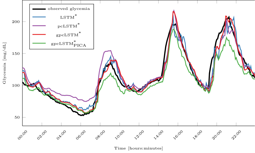
The gcMSE action is more focused on the decrease of the EP rate, as shown by the models gpcLSTM, gpcLSTM${}_{\text{CA}}$, gpcLSTM${}_{\text{PICA}}^{\text{*}}$. In contrast with the exponential smoothing technique and the cMSE cost function, the gcMSE improves all glycemic regions, and in particular the hypoglycemic region. Moreover, these improvements allow the LSTM neural network to surpass, in clinical acceptability, the SVR model which is the best model of the GLYFE benchmark study. Figure 3 allows us to appreciate the differences in the predictions of the different models. First, we can see the large variations and noise in the predicted glucose signal of the LSTM model. These oscillations are reduced for the other models, becoming closer to the observed glucose signal. However, when using the cMSE cost function (pcLSTM${}^{\text{*}}$ signal in purple), we witness a large loss of accuracy in the hypoglycemia region (between 4:00 and 8:00 am). While the signal gpcLSTM${}^{\text{*}}_{\text{PICA}}$ shows to be very close to the signal observed in the hypoglycemia region, this is done at the cost of an overall loss in accuracy. Finally, gpcLSTM${}^{\text{*}}$, is a compromise between the two.

(a) MASE evolution of the IDIAB patients

(b) MASE evolution of the OhioT1DM patients

(c) AP evolution of the IDIAB patients

(d) AP evolution of the OhioT1DM patients

(e) EP evolution of the IDIAB patients

(f) EP evolution of the OhioT1DM patients

Figure 4: Evolution of the MASE and CG-EGA (AP and EP) metrics throughout the PICA algorithm for the IDIAB and OhioT1DM datasets. Iterations 0 and 0^* respectively represent the results of the model trained with the MSE cost function before and after smoothing the predictions.

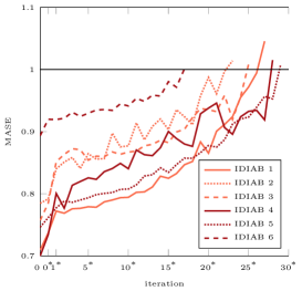
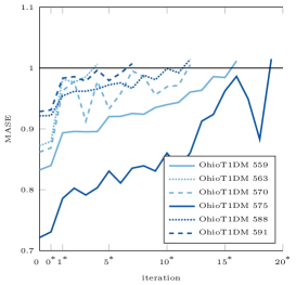
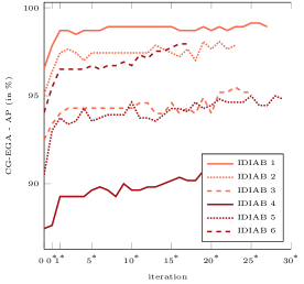
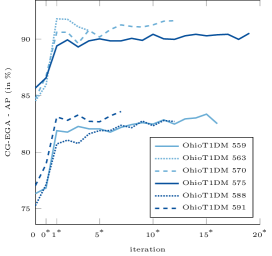
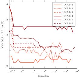
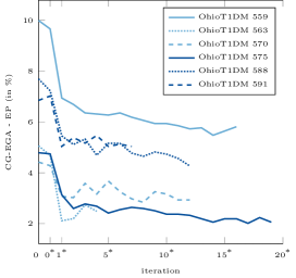
Although we can conclude on the strength of using the gcMSE cost function in the training of deep models predicting future glucose levels in people with diabetes, the different results show us that there are many possible tradeoffs between accuracy and clinical acceptability. The PICA algorithm proposed in this study aims at selecting the best compromise between accuracy and clinical acceptability based on selection criteria. Figure 4 gives a graphical representation of the changes in MASE, general AP rate and general EP rate of the models throughout the PICA algorithm for all the patients. As previously discussed, there is no clinical criterion for glucose predictive models yet, so the only criterion for stopping the algorithm here was the MASE exceeding 1. The figure first shows us that the number of iterations before stopping the algorithm is variable from one dataset to another, and also from one patient to another (25.0 $\pm$ 3.96 for the IDIAB dataset, and 11.66 $\pm$ 5.06 for the OhioT1DM dataset). This is explained first of all by the variable initial accuracy of the different patients, some patients being easier to predict than others (see iteration 0 on Figures 4(a) and 4(b)). As we have observed through the analysis of Table I, the main improvements in clinical acceptability are made at the first iteration (iteration 1) of the algorithm when introducing the gcMSE cost function and exponential smoothing. Nevertheless, throughout the algorithm, the clinical acceptability gradually improves at the expense of the accuracy. We can see that the rate of deterioration and improvement is different from one patient to another, showing the very high inter-patient variability in the diabetic population.

Although there is currently no clinical criterion for glucose prediction models, we can analyze the use of two hypothetical criteria through Table III: a minimum AP rate, and a maximum EP rate. As expected, the harder the clinical criteria (higher threshold and/or combination of criteria), the lower the number of patients passing the clinical test. Only one patient in the IDIAB dataset managed to have simultaneously more than 97% AP and less than 1% EP. In addition, we can note a greater success of IDIAB patients on these clinical tests, compared to OhioT1DM patients. As previously mentioned, these differences in clinical performance are due to the difference in experimental systems. While the final evaluation of the OhioT1DM dataset is done every 5 minutes, it is done every 15 minutes for the IDIAB dataset. In addition, the glucose signal of IDIAB patients is overall less noisy, and therefore more stable and easier to predict. Thus, for a future practical use, the clinical criteria must be rigorously standardized.

Finally, we note that the MASE on the testing set (the one reported in Tables I and II) is slightly higher than 1 (1.03 and 1.01 for the IDIAB and OhioT1DM datasets). Using such a stopping criterion, we could have assumed that the final MASE on the testing set would be less than 1, as it is the case on the validation set. This happens because the test subset is not fully representative of the validation subset. This is due to the general small quantities of data in the datasets, negatively impacting the representativeness of these subsets. We also note that the standard deviation for the IDIAB dataset is higher, showing that the final value of the MASE is highly variable depending on the subject. Thus, the accuracy of the PICA algorithm would be improved by using more data (which would also improve the performance of the models in general).

TABLE III: Number of patients within a given dataset that can respect different clinical criteria (minimal AP rate or maximal EP rate) through the PICA algorithm.

Clinical Criterion		Dataset
AP ($\geq$)	EP ($\leq$)	IDIAB	Ohio
80	-	6	6
90	-	6	3
95	-	4	0
97	-	3	0
-	7	6	6
-	5	6	4
-	3	6	3
-	1	4	0
80	7	6	6
90	5	6	3
95	3	4	0
97	1	2	0

III Conclusion

In this study, we proposed a framework for the integration of clinical criteria into the training of deep models. Clinical criteria are often different from standard statistical metrics used as loss functions. As a consequence the best model, given a loss function used during its training, is not necessarily the model with the best clinical acceptability. We address this issue from the perspective of the challenging task of predicting future glucose values of diabetic people.

In glucose prediction, the CG-EGA metric measures the clinical acceptability of the predictions. In particular, it assesses the safety of the predictions by looking at the prediction accuracy and the predicted rate of change accuracy. Moreover, the metric behaves differently for the different glycemic regions, some errors being more dangerous than others without being high amplitude errors. Starting from the cMSE loss function we proposed in an earlier work of ours [16] that penalizes the model during its training not only on prediction errors but also on predicted variation errors, we proposed to personalize the loss function to the glucose prediction task. Based on the CG-EGA, this personalization, called gcMSE, weights the errors differently depending on the scores obtained in the P-EGA and R-EGA grids. Finally, we proposed the PICA algorithm to obtain the solution that maximizes the accuracy of the model while at the same time respecting given clinical criteria.

We evaluate the different proposed loss functions and the PICA algorithm with two different diabetes datasets, the IDIAB and the OhioT1DM dataset. First, we showed that the cMSE loss function increase the coherence of successive predictions, improving the clinical acceptability of the models. However, this improvement comes at the cost of a decrease in the accuracy of the model. Then, we showed that the gcMSE further improves the clinical acceptability by reducing the rate of life-threatening errors. Finally, we demonstrate the usefulness of the PICA algorithm that help in choosing the desired tradeoff between general accuracy and clinical acceptability.

The analysis of different clinical criteria showed that not all the patients were able to meet them easily. It depends on the difficulty of the glucose prediction task of the patient, varying from patient to patient, but also on the nature of dataset, and in particular on the devices used for the data collection. These factors would need to be taken into account when creating future regulations for the use of such models by diabetic patients.

References

- [1] I. D. Federation, “Atlas du diabete de la fid neuvième édition 2019,” 2019. [Online]. Available: https://www.federationdesdiabetiques.org/
- [2] S. Oviedo, J. Vehí, R. Calm, and J. Armengol, “A review of personalized blood glucose prediction strategies for t1dm patients,” International journal for numerical methods in biomedical engineering, vol. 33, no. 6, p. e2833, 2017.
- [3] G. Sparacino, F. Zanderigo, S. Corazza, A. Maran, A. Facchinetti, and C. Cobelli, “Glucose concentration can be predicted ahead in time from continuous glucose monitoring sensor time-series,” IEEE Transactions on biomedical engineering, vol. 54, no. 5, pp. 931–937, 2007.
- [4] S. M. Pappada, B. D. Cameron, P. M. Rosman, R. E. Bourey, T. J. Papadimos, W. Olorunto, and M. J. Borst, “Neural network-based real-time prediction of glucose in patients with insulin-dependent diabetes,” Diabetes technology & therapeutics, vol. 13, no. 2, pp. 135–141, 2011.
- [5] E. I. Georga, V. C. Protopappas, D. Ardigò, D. Polyzos, and D. I. Fotiadis, “A glucose model based on support vector regression for the prediction of hypoglycemic events under free-living conditions,” Diabetes technology & therapeutics, vol. 15, no. 8, pp. 634–643, 2013.
- [6] J. B. Ali, T. Hamdi, N. Fnaiech, V. Di Costanzo, F. Fnaiech, and J.-M. Ginoux, “Continuous blood glucose level prediction of type 1 diabetes based on artificial neural network,” Biocybernetics and Biomedical Engineering, vol. 38, no. 4, pp. 828–840, 2018.
- [7] A. Aliberti, I. Pupillo, S. Terna, E. Macii, S. Di Cataldo, E. Patti, and A. Acquaviva, “A multi-patient data-driven approach to blood glucose prediction,” IEEE Access, vol. 7, pp. 69 311–69 325, 2019.
- [8] S. Mirshekarian, R. Bunescu, C. Marling, and F. Schwartz, “Using lstms to learn physiological models of blood glucose behavior,” in Engineering in Medicine and Biology Society (EMBC), 2017 39th Annual International Conference of the IEEE. IEEE, 2017, pp. 2887–2891.
- [9] S. Mirshekarian, H. Shen, R. Bunescu, and C. Marling, “Lstms and neural attention models for blood glucose prediction: Comparative experiments on real and synthetic data,” in 2019 41st Annual International Conference of the IEEE Engineering in Medicine and Biology Society (EMBC). IEEE, 2019, pp. 706–712.
- [10] J. Martinsson, A. Schliep, B. Eliasson, and O. Mogren, “Blood glucose prediction with variance estimation using recurrent neural networks,” Journal of Healthcare Informatics Research, pp. 1–18, 2019.
- [11] M. De Bois, M. A. E. Yacoubi, and M. Ammi, “Adversarial multi-source transfer learning in healthcare: Application to glucose prediction for diabetic people,” arXiv preprint arXiv:2006.15940, 2020.
- [12] T. Zhu, K. Li, P. Herrero, J. Chen, and P. Georgiou, “A deep learning algorithm for personalized blood glucose prediction.” in KHD@ IJCAI, 2018, pp. 64–78.
- [13] M. De Bois, M. Ammi, and M. A. E. Yacoubi, “Glyfe: Review and benchmark of personalized glucose predictive models in type-1 diabetes,” arXiv preprint arXiv:2006.15946, 2020.
- [14] S. Del Favero, A. Facchinetti, and C. Cobelli, “A glucose-specific metric to assess predictors and identify models,” IEEE transactions on biomedical engineering, vol. 59, no. 5, pp. 1281–1290, 2012.
- [15] B. P. Kovatchev, L. A. Gonder-Frederick, D. J. Cox, and W. L. Clarke, “Evaluating the accuracy of continuous glucose-monitoring sensors: continuous glucose–error grid analysis illustrated by therasense freestyle navigator data,” Diabetes Care, vol. 27, no. 8, pp. 1922–1928, 2004.
- [16] M. De Bois, M. A. El Yacoubi, and M. Ammi, “Prediction-coherent lstm-based recurrent neural network for safer glucose predictions in diabetic people,” in International Conference on Neural Information Processing. Springer, 2019, pp. 510–521.
- [17] C. Marling and R. C. Bunescu, “The ohiot1dm dataset for blood glucose level prediction.” in KHD@ IJCAI, 2018, pp. 60–63.
- [18] M. De Bois, “Integration of clinical criteria into the training of deep models: Application to glucose prediction for diabetic people,” 2020, doi: 10.5281/zenodo.3904234. [Online]. Available: https://github.com/dotXem/DeepClinicalGlucosePrediction
- [19] T.-Y. Lin, P. Goyal, R. Girshick, K. He, and P. Dollár, “Focal loss for dense object detection,” in Proceedings of the IEEE international conference on computer vision, 2017, pp. 2980–2988.
- [20] R. T. Marler and J. S. Arora, “Survey of multi-objective optimization methods for engineering,” Structural and multidisciplinary optimization, vol. 26, no. 6, pp. 369–395, 2004.
- [21] K. Deb, S. Agrawal, A. Pratap, and T. Meyarivan, “A fast elitist non-dominated sorting genetic algorithm for multi-objective optimization: Nsga-ii,” in International conference on parallel problem solving from nature. Springer, 2000, pp. 849–858.
- [22] R. J. Hyndman and A. B. Koehler, “Another look at measures of forecast accuracy,” International journal of forecasting, vol. 22, no. 4, pp. 679–688, 2006.
- [23] R. G. Brown, Smoothing, forecasting and prediction of discrete time series. Courier Corporation, 2004.
- [24] J. W. Taylor and P. E. McSharry, “Short-term load forecasting methods: An evaluation based on european data,” IEEE Transactions on Power Systems, vol. 22, no. 4, pp. 2213–2219, 2007.
- [25] C. Pérez-Gandía, A. Facchinetti, G. Sparacino, C. Cobelli, E. Gómez, M. Rigla, A. de Leiva, and M. Hernando, “Artificial neural network algorithm for online glucose prediction from continuous glucose monitoring,” Diabetes technology & therapeutics, vol. 12, no. 1, pp. 81–88, 2010.
- [26] M. De Bois, “Glyfe,” 2019, doi: 10.5281/zenodo.3234605. [Online]. Available: https://github.com/dotXem/GLYFE