Mixed QCD-electroweak corrections to $W$-boson production in hadron collisions

Abstract

We compute mixed QCD-electroweak corrections to the fully-differential production of an on-shell $W$ boson. Decays of $W$ bosons to lepton pairs are included in the leading order approximation. The required two-loop virtual corrections are computed analytically for arbitrary values of the electroweak gauge boson masses. Analytic results for integrated subtraction terms are obtained within a soft-collinear subtraction scheme optimized to accommodate the structural simplicity of infra-red singularities of mixed QCD-electroweak contributions. Numerical results for mixed corrections to the fiducial cross section of $pp\to W^{+}\to l^{+}\nu$ and selected kinematic distributions in this process are presented.

I Introduction

Studies of electroweak gauge bosons produced in hadron collisions played an important role in establishing the validity of the Standard Model of particle physics. Given these successes, it is not surprising that experiments at the LHC continue the systematic exploration of vector-boson production processes cms1 ; cms2 ; atlas1 ; atlas2 . Although plenty of interesting physics, ranging from constraints on parton distribution functions to measurements of the weak mixing angle to explorations of lepton universality, can be investigated by studying the production of single $W$ and $Z$ bosons, the Holy Grail of precision electroweak physics at the LHC is the measurement of the $W$-boson mass. Indeed, the current goal is to measure the $W$ mass with a precision of about $8\leavevmode\nobreak\$MeV to match the uncertainty in the value of the $W$ mass obtained from precision electroweak fits Baak:2014ora ; deBlas:2016ojx . If achieved, it will imply a relative uncertainty on the (directly measured) $W$-boson mass of about ${\cal O}(10^{-2})$ percent, an astounding precision.

Perturbative computations within the Standard Model play a central role in providing a precise description of $W$ and $Z$ production processes at the LHC and are thus crucial for the success of precision electroweak measurements. Currently, fully-differential cross sections for dilepton production in hadron collisions are known through next-to-next-to-leading order (NNLO) in perturbative QCD nnlo1 ; nnlo2 ; nnlo3 ; nnlo4 ; nnlo5 ; Caola:2019nzf ; nnlo7 ; nnlo8 ; nnlo9 ; nnlo10 ; nnlo11 and through next-to-leading order (NLO) in electroweak theory nloew1 ; nloew2 ; nloew3 ; nloew4 ; nloew5 ; nloew6 ; nloew7 ; nloew8 ; nloew9 ; nloew10 . Very recently, the total cross section for $W$ production was computed through N³LO in perturbative QCD Duhr:2020sdp .

Although an exact relation between the quality of the theoretical description of the process $pp\to W\to l\nu$ and the precision with which the $W$ mass can be extracted is complicated and observable-dependent, it is generally agreed that mixed QCD-electroweak corrections to this process, i.e. all effects that are suppressed by a product of QCD and electroweak couplings ${\cal O}(\alpha_{s}\alpha_{EW})$ relative to the leading-order process, need to be accounted for to achieve ${\cal O}(8)\leavevmode\nobreak\$MeV precision. It is also important to compute mixed corrections at a fully-differential level to ensure that they can be calculated for realistic observables.

Recently, such mixed QCD-electroweak corrections were calculated for on-shell $Z$ production at the LHC in Refs. Buccioni:2020cfi ; Bonciani:2020tvf , extending earlier results on mixed QCD-QED corrections presented in Refs. qcdqed ; deFlorian:2018wcj ; Cieri:2020ikq ; Bonciani:2019nuy . Although the underlying mechanisms for $Z$ and $W$ production at the LHC are quite similar, there are two outstanding issues with extending the computation of QCD-electroweak corrections to $W$ production. The first challenge is that two-loop mixed QCD-electroweak corrections are available for $Z$-boson production kkv but are unknown for the $W$-boson case. The computation of these corrections is cumbersome, since they depend on several mass scales, but definitely feasible. We present the results of this calculation in this paper.

The second problem that needs to be addressed are soft and collinear divergences. These divergences originate from singular soft and collinear limits of loop integrals and real-emission amplitudes; they are known to disappear when elastic and inelastic processes are combined. For the purpose of a fully-differential description of $W$ production in hadron collisions, these divergences need to be extracted from real-emission contributions without integration over the resolved phase space. Several ways to do this in practice were developed in the context of NNLO QCD computations at hadron colliders ant ; njet1 ; njet2 ; grazi ; Czakon:2010td ; Czakon:2014oma ; Cacciari:2015jma ; Caola:2017dug .

In this paper, we employ the so-called nested soft-collinear subtraction scheme Caola:2017dug that we adjust to accommodate particularities of mixed QCD-electroweak corrections. We note that such an adjustment was not necessary in the case of $Z$ production since $Z$ bosons are electrically neutral. For this reason, a simple abelianization of NNLO QCD corrections to $Z$ production was sufficient deFlorian:2018wcj . However, since $W$ bosons are electrically charged and, hence, interact with photons, it is not possible to adapt the NNLO QCD description of $W$ production to describe mixed QCD-electroweak corrections. In what follows, we derive simple formulas that describe integrated subtraction terms required to make ${\cal O}(\alpha_{s}\alpha_{EW})$ corrections to $pp\to W$ finite. Presenting these formulas, alongside results for the two-loop virtual corrections, is the main goal of this paper.

We note that mixed QCD-electroweak corrections to $pp\to W\to l\nu$ can be split into three categories: i) mixed corrections to the production process $pp\to W$, ii) QCD corrections to the production process and electroweak corrections to the decay and iii) non-factorizable corrections that connect production and decay processes ditt1 . The non-factorizable corrections to on-shell $W$ production are suppressed by powers of $\Gamma_{W}/M_{W}$ fadin ; ditt1 ; ditt2 and, therefore, can be neglected. Similarly, in case of on-shell production, corrections to the production and decay stages of the process can be defined unambiguously in a gauge-invariant way, see e.g. Ref. ditt1 . NLO QCD corrections to the production and NLO electroweak corrections to the decay – as well as mixed QCD-EW corrections to the decay coming from renormalization – have already been considered in Refs. ditt1 ; ditt2 and for this reason we do not consider them here. The unknown contribution is mixed QCD-electroweak corrections to the production process $pp\to W$ since it is of NNLO type. In this paper, we focus on this contribution.

More specifically, we derive formulas for the two-loop corrections to the $q\bar{q}^{\prime}\to W$ vertex function and for all the subtraction terms required to compute mixed QCD-electroweak corrections to $W$-boson production at the LHC. As an application, we provide results for fiducial cross sections and selected kinematic distributions for the $pp\to W^{+}\to l^{+}\nu$ process. However, we do not perform detailed phenomenological studies related to e.g. the impact of these corrections on the $W$-mass measurement since such studies warrant a separate publication. We plan to return to this topic in the near future.

The paper is organized as follows. In Section II we provide a brief overview of the nested soft-collinear subtraction scheme and point out differences between the mixed QCD-EW case studied here and the pure NNLO QCD cases considered earlier Caola:2017dug ; Caola:2019nzf . In Section III we describe the soft limits of scattering amplitudes relevant for computing mixed QCD-EW corrections. In Section IV we briefly discuss the computation of NLO electroweak corrections to $pp\to W$. In Section V we derive all of the integrated subtraction terms required for the full mixed QCD-EW calculation, focusing on the most complicated $q\bar{q}^{\prime}$ and $gq$ partonic channels. In Section VI we present final formulas for integrated subtraction terms for all partonic channels. In Section VII numerical results are presented. We conclude in Section VIII. Many intermediate results, including the detailed discussion of mixed QCD-electroweak corrections to the $q\bar{q}^{\prime}\to W$ form factor, are collected in the Appendices.

II An overview of the nested soft-collinear subtraction scheme and its modification for QCD-EW corrections to $W$ production

In this section, we provide an overview of the soft-collinear subtraction scheme Caola:2017dug ; Caola:2019nzf . For the sake of definiteness, we consider the process $pp\to W^{+}\to l^{+}\nu$. It is well-known that infra-red safe observables defined for this process must receive contributions from elastic $pp\to W^{+}(l^{+}\nu)$ and inelastic $pp\to W^{+}(l^{+}\nu)+X_{f}$ channels. We note that, depending on the type of corrections that are studied, $X_{f}$ stands for final states composed of gluons, quarks and/or photons.

It is conventional to use dimensional regularization to compute virtual corrections and to regulate real-emission contributions. In this case, higher-order contributions to the elastic process contain explicit $1/\epsilon$ poles that originate from an integration over loop momenta, whereas inelastic processes develop such $1/\epsilon$ poles only once the integration over phase spaces of all potentially unresolved particles is performed. To keep results fully-differential, this phase-space integration should be performed in a way that does not affect infra-red safe observables. A procedure that allows one to do that defines a particular computational scheme that is often referred to as a subtraction (or a slicing) scheme. As we already mentioned, in this paper we will use the so-called nested soft-collinear subtraction scheme introduced in Ref. Caola:2017dug .

The nested subtraction scheme is based on the well-known notion of factorization of scattering amplitudes in singular limits and the fact that, thanks to QCD color coherence, soft and collinear limits of scattering amplitudes can be dealt with independently of each other. The behavior of scattering amplitudes in the singular limits is well-known; typically, they split into universal functions that encapsulate singular behavior and amplitudes that describe lower-multiplicity processes.

The idea behind the soft-collinear subtraction scheme is to iteratively subtract such singular limits from differential cross sections starting from soft singularities. The subtraction terms have to be added back and integrated over the unresolved phase space. In the case of collinear singularities a similar procedure is followed; the collinear subtraction, however, applies to cross sections that are already soft-subtracted. This nested nature of the subtraction process gives rise to a name – the nested soft-collinear subtraction scheme.

An important challenge in constructing subtraction terms is to ensure that the resulting limits are unambiguous. This requires us to resolve overlapping singularities whenever they arise. In QCD overlapping singularities are present in both soft and collinear emissions but there is no soft-collinear overlap. To deal with soft singularities in QCD amplitudes, we order gluon energies and consider the so-called double-soft and single-soft limits. To deal with overlapping collinear singularities, we follow Refs. Frixione:1995ms ; Czakon:2010td and introduce partitions and sectors that allow us to uniquely specify how singular collinear limits are approached.

Although similar in spirit to the general QCD case, the calculation of mixed QCD-EW corrections to $q\bar{q}^{\prime}\to W^{+}$ is particular. There are a few reasons for that. The first one is that soft singularities in the process $q\bar{q}^{\prime}\to W^{+}g\gamma$ are not entangled. To understand this, we note that when both a gluon and a photon are emitted from quark lines, the situation is QED-like and soft singularities in QED are known to be independent from each other. If, however, a photon is emitted from a $W$-boson line and a gluon is emitted from a quark line, the independence of the two soft limits is obvious. This feature of mixed QCD-QED corrections allows us to consider soft limits of a photon and a gluon separately, leading to simplifications of the integrated subtraction terms compared to the QCD case. Indeed, only the product of two NLO-like integrated soft subtractions is required, although we need them to higher order in the $\epsilon$-expansion compared to a NLO calculation proper.

Similarly, collinear limits can be simplified because photons and gluons do not interact with each other. Since two out of the four collinear sectors described in Ref. Caola:2017dug for the NNLO QCD case are introduced to isolate the $g^{*}\to gg(q\bar{q})$ splitting, the mixed QCD-EW case can be simplified at least inasmuch as the $Wg\gamma$ final state is concerned. Moreover, for $gq$ initial states, the absence of $g\to g\gamma$ splittings leads to a simplified version of the required partition functions compared to the case discussed in Ref. Caola:2017dug , and a smaller number of singular limits that need to be considered. Contrary to the soft case, collinear sectors still contain genuine NNLO-like contributions that do not fully factorize into the product of NLO-like limits. Nevertheless, the features discussed above make the construction of subtraction terms much easier than in the generic QCD case.

As we already mentioned in the introduction, an important difference with respect to a computation of NNLO QCD corrections to $pp\to W$ Caola:2019nzf stems from the fact that $W$ bosons radiate photons. Since $W$ bosons are massive, such radiation does not affect collinear singularities but it does change the soft ones. Hence, formulas for the soft limits need to be modified compared to the QCD case. We describe the corresponding modifications and how we deal with them in the next section.

The final difference between the NNLO QCD computations reported in Refs. Caola:2017dug ; Caola:2019nzf and the one that we discuss in this paper is that this time we perform computations in an arbitrary, i.e. not center-of-mass, partonic reference frame. The very fact that the soft-collinear subtraction scheme is perfectly suited to deal with this situation in spite of the fact that it is not manifestly Lorentz invariant is interesting. It illustrates the flexibility of this approach and, on a practical level, it makes the treatment of soft and collinear limits very natural and transparent.

III The soft limits

As we mentioned in the previous section, an important difference between the computations of NNLO QCD and mixed QCD-electroweak corrections is the soft limits. In this section, we elaborate on this point and provide the required formulas to describe them.

The key feature that we exploit to construct soft subtraction terms for mixed QCD-EW corrections is the fact that soft-photon and soft-gluon limits are not entangled. For this reason we can consider the two soft limits independently. The resulting simplifications in computing integrated subtraction terms will become apparent when we discuss the NNLO computations in Section IV. In this section, we describe the soft limits relevant for the mixed case and explain how the required eikonal integrals can be evaluated.

We focus on the most complicated process $u(p_{1})+\bar{d}(p_{2})\to W^{+}+g(p_{4})+\gamma(p_{5})$. We employ notations that have been used in NNLO QCD calculations Caola:2017dug ; Caola:2019nzf and denote the product of the matrix element squared of this process and the relevant phase space factor for the $W$ boson (or its decay products) as $F_{\rm LM}(1_{u},2_{\bar{d}};4_{g},5_{\gamma})$

$$F_{\rm LM}(1_{u},2_{\bar{d}};4_{g},5_{\gamma})=\mathcal{N}\sum_{\rm col,pol}|\mathcal{A}(p_{1},p_{2};p_{W},p_{4},p_{5})|^{2}(2\pi)^{d}\delta_{d}(p_{1}+p_{2}-p_{W}-p_{4}-p_{5})\frac{\mathrm{d}^{d-1}p_{W}}{(2\pi)^{d-1}2E_{W}}.$$ (1)

A similar notation is used for lower-multiplicity processes. In Eq.(1), $\mathcal{N}$ stands for all the required ($d-$dimensional) initial-state color and helicity averaging factors, and for all the required final-state symmetry factors. Note that $F_{\rm LM}(1_{u},2_{\bar{d}};4_{g},5_{\gamma})$ does not contain the phase-space volume elements for the potentially unresolved particles $p_{4}$ and $p_{5}$. We consider the soft-gluon and the soft-photon limits separately. Similar to the NNLO QCD case, we describe these limits using two operators, $S_{g}$ and $S_{\gamma}$. The operator $S_{i}$ selects the most singular contribution of $|\mathcal{M}|^{2}$ in the $E_{i}\to 0$ limit and removes particle $i$ from the momentum-conserving $\delta$ function. For further details, see Refs. Caola:2017dug ; Caola:2019nzf .

We begin by considering the soft-gluon limit. In the notation that we have just reviewed, it reads

$$S_{g}F_{\rm LM}(1_{u},2_{\bar{d}};4_{g},5_{\gamma})=g_{s}^{2}\;{\rm Eik}_{g}(p_{1},p_{2};p_{4})F_{\rm LM}(1_{u},2_{\bar{d}};5_{\gamma}),$$ (2)

where $g_{s}$ is the (bare) strong coupling, and

$${\rm Eik}_{g}(p_{1},p_{2};p_{g})=\frac{2C_{F}(p_{1}p_{2})}{(p_{1}p_{g})(p_{2}p_{g})},$$ (3)

with $(p_{i}p_{j})\equiv p_{i}\cdot p_{j}$. Also, $C_{F}=(N_{c}^{2}-1)/(2N_{c})$ is the QCD quadratic Casimir and $N_{c}=3$ is the number of colors. Note that this limit is independent of whether or not there is a photon in the matrix element squared; this implies that an identical formula can be used to describe the soft gluon limit of the process $u(p_{1})+\bar{d}(p_{2})\to W^{+}+g(p_{4})$:

$$S_{g}F_{\rm LM}(1_{u},2_{\bar{d}};4_{g})=g_{s}^{2}\;{\rm Eik}_{g}(p_{1},p_{2};p_{4})F_{\rm LM}(1_{u},2_{\bar{d}}).$$ (4)

The soft-gluon limit of different partonic channels can be trivially obtained by crossing these results. For example,

$$S_{g}F_{\rm LM}(1_{\gamma},2_{\bar{d}};4_{\bar{u}},5_{g})=g_{s}^{2}\;{\rm Eik}_{g}(p_{2},p_{4};p_{5})F_{\rm LM}(1_{\gamma},2_{\bar{d}};4_{\bar{u}}).$$ (5)

To analyze the soft-photon limit, we write

$$S_{\gamma}F_{\rm LM}(1_{u},2_{\bar{d}};4_{g},5_{\gamma})=e^{2}\;{\rm Eik}_{\gamma}(p_{1},p_{2},p_{W};p_{5})F_{\rm LM}(1_{u},2_{\bar{d}};4_{g}),$$ (6)

where $p_{W}=p_{1}+p_{2}-p_{4}$ is the four-momentum of the $W$ boson and $e$ is the (bare) electric coupling. The QED eikonal function reads

$$\begin{split}{\rm Eik}_{\gamma}(p_{1},p_{2},p_{W};p_{\gamma})&=\left\{Q_{u}Q_{d}\frac{2(p_{1}p_{2})}{(p_{1}p_{\gamma})(p_{2}p_{\gamma})}-Q_{W}^{2}\frac{p_{W}^{2}}{(p_{W}p_{\gamma})^{2}}+Q_{W}\left(Q_{u}\frac{2(p_{W}p_{1})}{(p_{W}p_{\gamma})(p_{1}p_{\gamma})}-Q_{d}\frac{2(p_{W}p_{2})}{(p_{W}p_{\gamma})(p_{2}p_{\gamma})}\right)\right\}.\end{split}$$ (7)

In Eq.(7) we used $Q_{W}=Q_{u}-Q_{d}$ to denote the electric charge of the $W$ boson. Note that $p_{W}$ depends on the gluon four-momentum; hence, it changes if the soft-photon and the soft-gluon limits are considered simultaneously.

To compute the soft subtraction terms, we integrate the eikonal functions ${\rm Eik}_{g,\gamma}$ over the phase spaces of a soft gluon and/or photon. Following the NNLO QCD computations Caola:2017dug ; Caola:2019nzf we define phase-space elements with an upper energy cut-off $E_{\rm max}$

$$[{\rm d}p]=\frac{{\rm d}^{d-1}\vec{p}}{(2\pi)^{d-1}2p_{0}}\;\theta(E_{\rm max}-p_{0}).$$ (8)

In the case of the soft-gluon limit, we easily find

$$\int[{\rm d}p_{4}]g_{s}^{2}\;{\rm Eik}_{g}(p_{1},p_{2};p_{4})=[\alpha_{s}]\frac{2C_{F}(2E_{\rm max})^{-2\epsilon}}{\epsilon^{2}}\frac{\Gamma^{2}(1-\epsilon)}{\Gamma(1-2\epsilon)},$$ (9)

where

$$[\alpha_{s}]=\frac{g_{s}^{2}\Omega^{(d-2)}}{2(2\pi)^{d-1}}=\left(\frac{\alpha_{s}}{2\pi}\right)\frac{(4\pi)^{\epsilon}}{\Gamma(1-\epsilon)},$$ (10)

with $\alpha_{s}$ the (bare) strong coupling.

To describe the soft-photon contribution, we need to integrate the soft-photon eikonal function Eq.(7) over the photon phase space. Since this integral is more involved than the one in the gluon case Eq.(9), it is beneficial to compute it in two special cases.

The first case is that of a soft photon but resolved gluon. The relevant eikonal integral was computed in Ref. Alioli:2010xd and we borrow it from there. We obtain

$$\int[{\rm d}p_{5}]e^{2}{\rm Eik}_{\gamma}(p_{1},p_{2},p_{W};p_{5})=[\alpha](2E_{\rm max})^{-2\epsilon}\frac{\Gamma^{2}(1-\epsilon)}{\Gamma(1-2\epsilon)}J_{\gamma}(1,2,W),$$ (11)

where

$$\begin{split}&J_{\gamma}(1,2,W)=\frac{Q_{d}^{2}+Q_{u}^{2}}{\epsilon^{2}}+\frac{Q_{W}}{\epsilon}\left(Q_{W}-2Q_{u}\ln\left(\frac{\kappa_{1W}}{\sqrt{1-\beta^{2}}}\right)+2Q_{d}\ln\left(\frac{\kappa_{2W}}{\sqrt{1-\beta^{2}}}\right)\right)\\ &-Q_{W}^{2}\left[\frac{1}{\beta}\ln\frac{1-\beta}{1+\beta}-\frac{1}{2}\ln^{2}\frac{1-\beta}{1+\beta}\right]-2Q_{W}\sum\limits_{i=1}^{2}Q_{i}(-1)^{i}\ln\left(\frac{\kappa_{iW}}{1-\beta}\right)\ln\left(\frac{\kappa_{iW}}{1+\beta}\right)\\ &-2Q_{W}\sum\limits_{i=1}^{2}Q_{i}(-1)^{i}\left[{\rm Li}_{2}\left(1-\frac{\kappa_{iW}}{1-\beta}\right)+{\rm Li}_{2}\left(1-\frac{\kappa_{iW}}{1+\beta}\right)\right]+\mathcal{O}(\epsilon).\end{split}$$ (12)

In Eq.(12) $Q_{1}=Q_{u}$ and $Q_{2}=Q_{d}$, $Q_{W}=Q_{u}-Q_{d}$, $\beta=\sqrt{1-M_{W}^{2}/E_{W}^{2}}$ and $\kappa_{iW}=(p_{i}p_{W})/(E_{i}E_{W})$. Note that, similar to the QCD case, we introduced in Eq.(11) a convenient notation for the (bare) fine structure constant $\alpha$

$$[\alpha]=\frac{e^{2}\Omega^{(d-2)}}{2(2\pi)^{d-1}}=\left(\frac{\alpha}{2\pi}\right)\frac{(4\pi)^{\epsilon}}{\Gamma(1-\epsilon)}.$$ (13)

For the gluon-initiated process $g(p_{1})+\bar{d}(p_{2})\to W^{+}+\bar{u}(p_{4})+\gamma(p_{5})$, we require a similar but slightly different integrated eikonal function. It reads

$$\int[{\rm d}p_{5}]e^{2}{\rm Eik}_{\gamma}(p_{2},p_{4},p_{W};p_{5})=[\alpha](2E_{\rm max})^{-2\epsilon}\frac{\Gamma^{2}(1-\epsilon)}{\Gamma(1-2\epsilon)}\;J_{\gamma}(2,4,W),$$ (14)

where

$$\begin{split}&J_{\gamma}(2,4,W)=\frac{Q_{d}^{2}+Q_{u}^{2}}{\epsilon^{2}}+\frac{Q_{W}}{\epsilon}\left(Q_{W}-2Q_{u}\ln\left(\frac{\kappa_{4W}}{\sqrt{1-\beta^{2}}}\right)+2Q_{d}\ln\left(\frac{\kappa_{2W}}{\sqrt{1-\beta^{2}}}\right)\right)-\frac{2Q_{u}Q_{d}}{\epsilon}\ln(\eta_{42})\\ &-Q_{W}^{2}\left[\frac{1}{\beta}\ln\frac{1-\beta}{1+\beta}-\frac{1}{2}\ln^{2}\frac{1-\beta}{1+\beta}\right]-2Q_{W}\sum\limits_{i\in\{2,4\}}Q_{i}\ln\left(\frac{\kappa_{iW}}{1-\beta}\right)\ln\left(\frac{\kappa_{iW}}{1+\beta}\right)\\ &-2Q_{W}\sum\limits_{i\in\{2,4\}}Q_{i}\left[{\rm Li}_{2}\left(1-\frac{\kappa_{iW}}{1-\beta}\right)+{\rm Li}_{2}\left(1-\frac{\kappa_{iW}}{1+\beta}\right)\right]+2Q_{d}Q_{u}\left({\rm Li}_{2}(1-\eta_{42})+\frac{1}{2}\ln^{2}\eta_{42}\right)+\mathcal{O}(\epsilon),\end{split}$$ (15)

and $Q_{2}=Q_{d}$, $Q_{4}=-Q_{u}$, $Q_{W}=Q_{u}-Q_{d}$, $\beta=\sqrt{1-M_{W}^{2}/E_{W}^{2}}$ and $\kappa_{iW}=p_{i}p_{W}/(E_{i}E_{W})$. We also used $\eta_{42}=(p_{2}p_{4})/(2E_{2}E_{4})=(1-\cos\theta_{42})/2$ in Eq.(15).

We can use the integrated soft-photon eikonal factors shown in Eqs.(11,14) both when a gluon or a quark in the final state are resolved, so that $p_{W}\neq p_{1}+p_{2}$, and when they are unresolved. However, for the latter case one needs to evaluate the integrated photon eikonal function to higher orders in the $\epsilon$-expansion, in the required kinematic configuration. It is technically more convenient to obtain this result by first taking the required limits in the eikonal function Eq.(7) and integrating over the photon four-momentum after that, rather than the other way around.

Although soft and collinear parton emissions have a different impact on the QED eikonal function, it is easy to see that we can accommodate both soft and collinear limits of the emitted parton $p_{4}$ by integrating the eikonal function ${\rm Eik}_{\gamma}$ in an arbitrary reference frame with the constraint $p_{W}=p_{1}+p_{2}$. We write such an integral as

$$\int[{\rm d}p_{5}]\;e^{2}{\rm Eik}_{\gamma}(p_{1},p_{2},p_{W};p_{5})|_{p_{W}=p_{1}+p_{2}}=[\alpha](2E_{\rm max})^{-2\epsilon}\frac{\Gamma^{2}(1-\epsilon)}{\Gamma(1-2\epsilon)}{\tilde{J}}_{\gamma}(E_{1},E_{2}),$$ (16)

where the function ${\tilde{J}}_{\gamma}(E_{1},E_{2})$ reads

$$\begin{split}{\tilde{J}}_{\gamma}(E_{1},E_{2})&=\frac{Q_{u}^{2}+Q_{d}^{2}}{\epsilon^{2}}+\frac{Q_{W}^{2}}{\epsilon(1-2\epsilon)}+\frac{Q_{W}}{\epsilon^{2}}\left\{Q_{u}\left[\left(\frac{E_{1}}{E_{2}}\right)^{\epsilon}-1\right]-Q_{d}\left[\left(\frac{E_{2}}{E_{1}}\right)^{\epsilon}-1\right]\right\}\\ &+\frac{Q_{W}}{\epsilon^{2}}\left\{Q_{u}\left(\frac{E_{1}}{E_{2}}\right)^{\epsilon}\left[F_{21}\left(-\epsilon,-2\epsilon,1-2\epsilon,1-\frac{E_{2}}{E_{1}}\right)-1\right]\right.\\ &\left.-Q_{d}\left(\frac{E_{2}}{E_{1}}\right)^{\epsilon}\left[F_{21}\left(-\epsilon,-2\epsilon,1-2\epsilon,1-\frac{E_{1}}{E_{2}}\right)-1\right]\right\}\\ &+\frac{Q_{W}^{2}}{\epsilon(1-2\epsilon)}\left(\frac{E_{2}}{E_{1}}\right)^{\epsilon}\left[F_{21}\left(-2\epsilon,1-\epsilon,2-2\epsilon,1-\frac{E_{1}}{E_{2}}\right)-1\right].\end{split}$$ (17)

We note that entries in the first line in Eq.(17) are divergent contributions to ${\tilde{J}}_{\gamma}$; all other terms in Eq.(17) have a finite $\epsilon\to 0$ limit. We also note that the function ${\tilde{J}}_{\gamma}$ assumes a particularly simple form in the partonic center-of-mass frame, $E_{1}=E_{2}$. We find

$${\tilde{J}}_{\gamma}(E_{1},E_{1})=\frac{Q_{u}^{2}+Q_{d}^{2}}{\epsilon^{2}}+\frac{Q_{W}^{2}}{\epsilon(1-2\epsilon)}.$$ (18)

Although, as we said earlier, we perform all computations in an arbitrary frame, once the poles cancellation is achieved, we switch back to the partonic center-of-mass frame to present analytic results for the finite integrated subtraction terms. The simplicity of Eq.(18) is an important reason to expect results in the center-of-mass frame to be compact and physically transparent.

IV Next-to-leading order electroweak corrections

To introduce notations and show how the nested soft-collinear subtraction scheme is applied to a simple problem, we briefly discuss the computation of NLO electroweak corrections. At this order, we need to consider both the $q\bar{q}^{\prime}\to W\gamma$ and the $\gamma q\to Wq^{\prime}$ channels.

We first consider the $q\bar{q}^{\prime}$ channel, and begin with the real-emission process $u(p_{1})+\bar{d}(p_{2})\to W^{+}+\gamma(p_{4})$. Using the notation introduced in Ref. Caola:2017dug and reviewed in the previous section, we write the real-emission contribution as

$$2s\cdot{\rm d}\sigma^{\gamma}_{R}=\int[{\rm d}p_{4}]F_{\rm LM}(1_{u},2_{\bar{d}};4_{\gamma})=\langle F_{\rm LM}(1_{u},2_{\bar{d}};4_{\gamma})\rangle,$$ (19)

where $s=2p_{1}\cdot p_{2}$ and $[{\rm d}p_{4}]={\rm d}^{d-1}p_{4}/((2\pi)^{d-1}2E_{4})\theta(E_{\rm max}-E_{4})$. We do not show the four-momentum of the $W$ boson in the list of arguments of the function $F_{\rm LM}$; we assume that it is always derived from energy-momentum conservation. We note that the phase-space integration measure for all final-state particles but the photon, as well as the delta function that ensures energy-momentum conservation, are included in the function $F_{\rm LM}$, see Eq.(1).

We begin with the extraction of soft singularities and write

$$\langle F_{\rm LM}(1_{u},2_{\bar{d}};4_{\gamma})\rangle=\langle S_{\gamma}F_{\rm LM}(1_{u},2_{\bar{d}};4_{\gamma})\rangle+\langle(I-S_{\gamma})F_{\rm LM}(1_{u},2_{\bar{d}};4_{\gamma})\rangle.$$ (20)

The first term in Eq.(20) is computed using the integrated eikonal function given in Eq.(16). We find

$$\langle S_{\gamma}F_{\rm LM}(1_{u},2_{\bar{d}};4_{\gamma})\rangle=[\alpha](2E_{\rm max})^{-2\epsilon}\frac{\Gamma^{2}(1-\epsilon)}{\Gamma(1-2\epsilon)}\langle{\tilde{J}}_{\gamma}(E_{1},E_{2})F_{\rm LM}(1_{u},2_{\bar{d}})\rangle.$$ (21)

The term proportional to $(I-S_{\gamma})$ on the right hand side of Eq.(20) is soft-regulated, but it still contains divergences when the photon becomes collinear to one of the incoming quarks. To regulate them, we use the same approach we used for the QCD case Caola:2017dug ; Caola:2019nzf . In particular, in analogy to the soft case we introduce the collinear operators $C_{\gamma i}$ that extract the collinear limit from $F_{\rm LM}$, see Refs. Caola:2017dug ; Caola:2019nzf for details. We then write

$$\langle(I-S_{\gamma})F_{\rm LM}(1_{u},2_{d};4_{\gamma})\rangle=\langle{\cal O}_{\rm NLO}^{\gamma}\left[F_{\rm LM}(1_{u},2_{d};4_{\gamma})\right]\rangle+\langle(I-S_{\gamma})\left(C_{\gamma 1}+C_{\gamma 2}\right)F_{\rm LM}(1_{u},2_{d};4_{\gamma})\rangle,$$ (22)

where ${\cal O}_{\rm NLO}^{\gamma}=(I-S_{\gamma})\left(I-C_{\gamma 1}-C_{\gamma 2}\right)$. The first term on the right hand side of Eq.(22) is fully regulated and we do not discuss it anymore. In the last two terms, we need to consider the limit when the photon becomes collinear to either $p_{1}$ or $p_{2}$. We start with the case when the photon is collinear to $p_{1}$. The corresponding collinear limit can be directly taken from the QCD case Caola:2017dug ; Caola:2019nzf . We obtain

$$C_{\gamma 1}F_{\rm LM}(1_{u},2_{d};4_{\gamma})=\frac{e^{2}Q_{u}^{2}}{E_{4}^{2}\rho_{41}}\left(1-z\right){\bar{P}}_{qq}(z)\frac{F_{\rm LM}(z\cdot 1_{u},2_{\bar{d}})}{z},$$ (23)

where $E_{4}=(1-z)E_{1}$, $\rho_{ij}=p_{i}\cdot p_{j}/(E_{i}E_{j})=1-\cos\theta_{ij}$ and the splitting function ${\bar{P}}_{qq}(z)$ is defined as follows

$${\bar{P}}_{qq}(z)=\frac{1+z^{2}}{1-z}-\epsilon(1-z).$$ (24)

Note that compared to a conventional $q\to q+g$ splitting function, we do not include the color factor $C_{F}$ in ${\bar{P}}_{qq}$. The reason for that is that one and the same splitting function can then be used to describe both the $q\to q+\gamma$ and $q\to q+g$ splittings which is quite convenient.

The next steps are identical to the QCD computation and involve integration over the photon emission angle in the soft-regulated collinear term Caola:2017dug ; Caola:2019nzf . Repeating these steps, we find

$$\langle(I-S_{\gamma})C_{\gamma 1}F_{\rm LM}(1_{u},2_{d};4_{\gamma})=-[\alpha]\frac{Q_{u}^{2}}{\epsilon}\frac{\Gamma^{2}(1-\epsilon)}{\Gamma(1-2\epsilon)}\left\langle(2E_{1})^{-2\epsilon}\int\limits_{0}^{1}{\rm d}zP_{qq}^{\rm NLO}(z,L_{1})\frac{F_{\rm LM}\left(z\cdot 1_{u},2_{\bar{d}}\right)}{z}\right\rangle,$$ (25)

where $L_{1}=\ln E_{\rm max}/E_{1}$ and

$$P_{qq}^{\rm NLO}(z,L)=(1-z)^{-2\epsilon}{\bar{P}}_{qq}(z)+\frac{1}{\epsilon}\delta(1-z)e^{-2\epsilon L}.$$ (26)

The expansion of the function $P_{qq}^{\rm NLO}$ in powers of $\epsilon$ is given in Appendix C.

To obtain the final result for the soft-regulated collinear contribution in Eq.(22) we need to account for the term proportional to $C_{\gamma 2}(I-S_{\gamma})$. It is easy to obtain it from Eq.(25) by replacing $L_{1}$ with $L_{2}=\ln E_{\rm max}/E_{2}$ and $F_{\rm LM}\left(z\cdot 1_{u},2_{\bar{d}}\right)$ with $F_{\rm LM}\left(1_{u},z\cdot 2_{\bar{d}}\right)$. Upon doing that, we find

$$\begin{split}&2s\cdot{\rm d}\sigma^{\gamma}_{R}=[\alpha](2E_{\rm max})^{-2\epsilon}\frac{\Gamma^{2}(1-\epsilon)}{\Gamma(1-2\epsilon)}\langle{\tilde{J}}_{\gamma}(E_{1},E_{2})\;F_{\rm LM}(1_{u},2_{\bar{d}})\rangle+\left\langle{\cal O}_{\rm NLO}^{\gamma}\left[F_{\rm LM}(1_{u},2_{\bar{d}};4_{\gamma})\right]\right\rangle\\ &-\frac{[\alpha]}{\epsilon}\frac{\Gamma^{2}(1-\epsilon)}{\Gamma(1-2\epsilon)}\int\limits_{0}^{1}{\rm d}z\sum\limits_{i=1}^{2}Q_{i}^{2}(2E_{i})^{-2\epsilon}P_{qq}^{\rm NLO}(z,L_{i})\left\langle F^{(i)}_{\rm LM}\left(1_{u},2_{\bar{d}}\;|\;z\right)\right\rangle,\end{split}$$ (27)

where we used the notation $Q_{1,2}=Q_{u,d}$ and

$$F^{(i)}_{\rm LM}\left(1_{u},2_{\bar{d}}\;|\;z\right)=\left\{\begin{array}[]{cc}F_{\rm LM}\left(z\cdot 1_{u},2_{\bar{d}}\right)/z,&i=1,\\ F_{\rm LM}\left(1_{u},z\cdot 2_{\bar{d}}\right)/z,&i=2.\\ \end{array}\right.$$ (28)

We will use the notation in Eq.(28) and its natural generalizations in what follows.

To obtain the final result for the NLO corrections, we have to combine the real-emission contribution Eq.(27) with virtual corrections and PDFs renormalization. The former are discussed in Appendix A. We now discuss the latter. Collinear counterterms depend on the renormalized coupling constant $\alpha(\mu)$. Since all the above results are written using unrenormalized couplings, we rewrite the results for the convolutions through the unrenormalized coupling constants as well using

$$[\alpha(\mu)]=\frac{\Gamma(1-\epsilon)}{\mu^{2\epsilon}e^{\epsilon\gamma_{E}}}\;[\alpha],\;\;\;\;[\alpha_{s}(\mu)]=\frac{\Gamma(1-\epsilon)}{\mu^{2\epsilon}e^{\epsilon\gamma_{E}}}\;[\alpha_{s}].$$ (29)

The collinear renormalization contribution then reads

$${\rm d}\sigma_{\rm pdf}=\frac{[\alpha]}{\epsilon}\frac{\Gamma(1-\epsilon)}{\mu^{2\epsilon}e^{\epsilon\gamma_{E}}}\int{\rm d}z\;{\bar{P}}_{qq}^{{\rm AP},0}(z)\sum\limits_{i=1}^{2}Q_{i}^{2}\left\langle F^{(i)}_{\rm LM}\left(1_{u},2_{\bar{d}}\;|\;z\right)\right\rangle,$$ (30)

where ${\bar{P}}_{qq}^{{\rm AP},0}$ is the (color-stripped) LO Altarelli-Parisi splitting function. Its explicit form is given in Appendix D.

Combining virtual and real contributions with the collinear renormalization contribution we find the final result for NLO electroweak corrections to the $u+\bar{d}\to W^{+}$ process. It reads

$$\begin{split}2s\cdot{\rm d}&\sigma^{\rm EW}_{{\rm NLO},q\bar{q}^{\prime}}=\left\langle F_{\rm LV}^{\rm EW,fin}(1_{u},2_{\bar{d}})+{\cal O}_{\rm NLO}^{\gamma}\left[F_{\rm LM}(1_{u},2_{\bar{d}};4_{\gamma})\right]\right\rangle+[\alpha]\int\limits_{0}^{1}{\rm d}z\;\sum\limits_{i=1}^{2}Q_{i}^{2}P_{qq}^{\rm fin}(z,E_{i})\left\langle F^{(i)}_{\rm LM}(1_{u},2_{\bar{d}}\;|\;z)\right\rangle\\ &+[\alpha]\left\langle\left[-\frac{Q_{u}^{2}+Q_{d}^{2}}{\epsilon^{2}}-\frac{1}{\epsilon}\left(\frac{5}{2}(Q_{u}^{2}+Q_{d}^{2})-2Q_{u}Q_{d}\right)+Q_{u}Q_{d}\big{[}1-\cos(\pi\epsilon)\big{]}\left(\frac{2}{\epsilon^{2}}+\frac{3}{\epsilon}\right)\right]s_{12}^{-\epsilon}F_{\rm LM}(1_{u},2_{\bar{d}})\right\rangle\\ &+[\alpha]\frac{\Gamma^{2}(1-\epsilon)}{\Gamma(1-2\epsilon)}\left\langle(2E_{\rm max})^{-2\epsilon}{\tilde{J}}_{\gamma}(E_{1},E_{2})+\sum\limits_{i=1}^{2}\left\{\frac{Q_{i}^{2}(2E_{i})^{-2\epsilon}}{\epsilon}\left[\frac{3}{2}+\frac{1}{\epsilon}\left(1-e^{-2\epsilon L_{i}}\right)\right]\right\}F_{\rm LM}(1_{u},2_{\bar{d}})\right\rangle,\end{split}$$ (31)

where $F_{\rm LV}^{\rm EW,fin}$ is defined in Appendix A. The splitting function $P^{\rm fin}_{qq}(z,E_{i})$ is defined in the following way

$$P_{qq}^{\rm fin}(z,E_{i})=-\frac{1}{\epsilon}\left[\frac{\Gamma^{2}(1-\epsilon)}{\Gamma(1-2\epsilon)}(2E_{i})^{-2\epsilon}\left(P_{qq}^{\rm NLO}(z,0)+\frac{3}{2}\delta(1-z)\right)-\frac{\Gamma(1-\epsilon)}{e^{\epsilon\gamma_{E}}\mu^{2\epsilon}}\bar{P}_{qq}^{{\rm AP},0}(z)\right].$$ (32)

The representation of the NLO cross section as in Eq.(31) is convenient as it allows us to compute convolutions of these cross sections with splitting functions, required for the evaluation of mixed QCD-EW corrections, in a straightforward way. It is easy to check that, upon expanding in $\epsilon$, all singularities in Eq.(31) cancel and a finite result is obtained. In the center-of-mass frame $E_{1}=E_{2}$ and with $\mu=M_{W}$, $E_{\rm max}=E_{1}$, Eq.(31) becomes

$$\begin{split}&2s\cdot\mathrm{d}\sigma^{\rm EW}_{{\rm NLO},q\bar{q}^{\prime}}=\\ &+\left(\frac{\alpha_{EW}}{2\pi}\right)\Bigg{\{}\int\limits_{0}^{1}\mathrm{d}z\sum_{i=1}^{2}Q_{i}^{2}\mathcal{P}_{qq}^{\rm NLO}(z)\left\langle F^{(i)}_{\rm LM}(1_{u},2_{\bar{d}}\;|\;z)\right\rangle+\left[\frac{\pi^{2}}{3}\left(Q_{u}^{2}+Q_{d}^{2}\right)+\left(2-\frac{\pi^{2}}{2}\right)Q_{W}^{2}\right]\langle F_{\rm LM}(1_{u},2_{\bar{d}})\rangle\Bigg{\}}\\ &+\left\langle F_{\rm LV}^{\rm EW,fin}(1_{u},2_{\bar{d}})+{\cal O}_{\rm NLO}^{\gamma}\left[F_{\rm LM}(1_{u},2_{\bar{d}};4_{\gamma})\right]\right\rangle+\mathcal{O}(\epsilon).\end{split}$$ (33)

In Eq.(33), $\alpha_{EW}$ is the renormalized coupling and we have introduced

$$\mathcal{P}_{qq}^{\rm NLO}(z)=4\left[\frac{\ln(1-z)}{1-z}\right]_{+}-2(1+z)\ln(1-z)+(1-z)-\frac{1+z^{2}}{1-z}\ln z.$$ (34)

The extraction of singularities in the $\gamma q\to Wq^{\prime}$ channel proceeds in full analogy with the discussion above and, for this reason, we do not repeat it here and limit ourselves to presenting the final result. For definiteness, we consider the $\gamma\bar{d}\to W^{+}\bar{u}$ channel, work in the center-of-mass frame and set $\mu=M_{W}$, $E_{\rm max}=E_{1}=E_{2}$. We obtain

$$2s\cdot\mathrm{d}\sigma^{\rm EW}_{{\rm NLO},\gamma q}=[\alpha]\int\limits_{0}^{1}\mathrm{d}zN_{c}Q_{u}^{2}P_{qg}^{\rm fin}(z,E_{1})\left\langle\frac{F_{\rm LM}(z\cdot 1_{u},2_{\bar{d}})}{z}\right\rangle+\left\langle{\cal O}_{\rm NLO}^{\bar{u}}\left[F_{\rm LM}(1_{\gamma},2_{\bar{d}};4_{\bar{u}})\right]\right\rangle,$$ (35)

where ${\cal O}_{\rm NLO}^{\bar{u}}=I-C_{41}$. We also defined

$$P_{qg}^{\rm fin}(z,E_{i})=-\frac{1}{\epsilon}\left[\frac{\Gamma^{2}(1-\epsilon)}{\Gamma(1-2\epsilon)}(2E_{i})^{-2\epsilon}P_{qg}^{\rm NLO}(z)-\frac{\Gamma(1-\epsilon)}{e^{\epsilon\gamma_{E}}\mu^{2\epsilon}}\bar{P}_{qg}^{{\rm AP},0}(z)\right],$$ (36)

with $\bar{P}_{qg}^{{\rm AP},0}(z)$ defined in Appendix D and

$$P_{qg}^{\rm NLO}(z)=(1-z)^{-2\epsilon}\big{[}(1-z)^{2}+z^{2}-\epsilon\big{]}/(1-\epsilon).$$ (37)

We note that the factor $1/(1-\epsilon)$ appears because the averaging factors of hard processes, included in the definition of hard functions $F_{\rm LM},$ are different for processes with different initial states. In case of Eq.(35), the left hand side involves a gluon-quark cross section where the overall factor includes an average over $(d-2)=2(1-\epsilon)$ gluon polarizations; on the right hand side of Eq.(35) the cross section for quark-antiquark annihilation appears where an average over the two quark (antiquark) polarizations is included. The mismatch between polarizations of gluons and quarks in the initial state leads to the factor $(1-\epsilon)$ that appears explicitly in our definition of $P_{qg}^{\rm NLO}$.

After expanding in $\epsilon$, we obtain

$$\begin{split}2s\cdot\mathrm{d}\sigma^{\rm EW}_{{\rm NLO},\gamma q}&=\left(\frac{\alpha_{EW}}{2\pi}\right)\int\limits_{0}^{1}\mathrm{d}zN_{c}Q_{u}^{2}\mathcal{P}_{qg}^{\rm NLO}(z)\left\langle\frac{F_{\rm LM}(z\cdot 1_{u},2_{\bar{d}})}{z}\right\rangle+\left\langle{\cal O}_{\rm NLO}^{\bar{u}}\left[F_{\rm LM}(1_{\gamma},2_{\bar{d}};4_{\bar{u}})\right]\right\rangle+\mathcal{O}(\epsilon),\end{split}$$ (38)

with

$$\mathcal{P}_{qg}^{\rm NLO}(z)=\big{[}z^{2}+(1-z)^{2}\big{]}\ln\left(\frac{(1-z)^{2}}{z}\right)+2z(1-z).$$ (39)

Although Eqs.(33,38) are written for $\mu=M_{W}$, the full scale dependence can be easily restored using renormalization-group arguments.

V Mixed QCD-EW corrections at next-to-next-to-leading order: derivation

The purpose of this section is to describe the computation of all the relevant contributions to mixed QCD-electroweak corrections. At this order, five partonic channels ($q\bar{q}^{\prime}$, $gq$, $\gamma q$, $\gamma g$, $qq^{\prime}$) contribute. In this section, we focus on the first two channels. The reason for this is that the $\gamma q$ channel can be obtained with manipulations similar (but simpler) to the ones for the $gq$ channel. The $\gamma g$ and $qq^{\prime}$ channels can readily be obtained by a simple abelianization deFlorian:2018wcj of the QCD result Caola:2017dug ; Caola:2019nzf . For completeness, we will present final formulas for all the channels in the next section.

This section is organized as follows: in Section V.1 we discuss in detail the double-real contribution to the $q\bar{q}^{\prime}$ channel, the most challenging part of the calculation. In Section V.2 we briefly explain how to derive all the other required contributions for the $q\bar{q}^{\prime}$ channel. Finally, in Section V.3 we discuss the $gq$ channel.

V.1 The $q\bar{q}^{\prime}$ channel: double-real contribution

To illustrate the main differences with respect to the earlier NNLO QCD computations  Caola:2017dug ; Caola:2019nzf , we consider a real-emission process $u(p_{1})+\bar{d}(p_{2})\to W^{+}f_{1}(p_{4})f_{2}(p_{5})$ and explain how to construct subtraction terms and how to integrate them over unresolved phase spaces. As mentioned earlier, we work in an arbitrary reference frame. In principle, we need to consider two options: either $(f_{1},f_{2})=(g,\gamma)$ or $(f_{1},f_{2})=(q,\bar{q})$. However, the singularity structure of the second contribution is very simple: since at $\mathcal{O}(\alpha_{s}\alpha_{EW})$ the two-quark final states only contribute through a $s$- and $t$-channel interference (see Fig. 1) the matrix element is only singular in triple collinear configurations $p_{4}||p_{5}||p_{i}$, $i=1,2$. These configurations can be dealt with by abelianizing the corresponding QCD result Caola:2017dug ; Caola:2019nzf . For this reason, we do not discuss it here and focus our attention on the $(f_{1},f_{2})=(g,\gamma)$ final state.

Figure 1: Two-quark final state contribution to the $q\bar{q}^{\prime}$ channel. In both Feynman graphs, the internal vector boson can be either a gluon or a $\gamma/W/Z$. Left: representative of $s$-channel diagram. Right: representative of $t$-channel diagram. Because of color conservation, only the $s$/$t$ interference leads to a non-vanishing contribution at $\mathcal{O}(\alpha_{s}\alpha_{EW})$.

We write the cross section for the partonic sub-process $u(p_{1})+\bar{d}(p_{2})\to W^{+}+g(p_{4})+\gamma(p_{5})$ as follows

$$2s\cdot{\rm d}\sigma_{RR}^{g\gamma}=\int[{\rm d}p_{4}][{\rm d}p_{5}]F_{\rm LM}(1_{u},2_{\bar{d}}\;;4_{g},5_{\gamma})=\langle F_{\rm LM}(1_{u},2_{\bar{d}}\;;4_{g},5_{\gamma})\rangle.$$ (40)

As discussed in Section II, we do not order gluon and photon energies since there are no entangled singularities in the kinematic limit when both of these particles become soft.

Similar to the NNLO QCD case, we first isolate soft singularities. We write

$$\begin{split}\langle F_{\rm LM}(1_{u},2_{\bar{d}};4_{g},5_{\gamma})\rangle&=\langle S_{\gamma}S_{g}\;F_{\rm LM}(1_{u},2_{\bar{d}}\;;4_{g},5_{\gamma})\rangle\\ &+\langle\left((I-S_{g})S_{\gamma}+(I-S_{\gamma})S_{g}\right)\;F_{\rm LM}(1_{u},2_{\bar{d}}\;;4_{g},5_{\gamma})\rangle\\ &+\langle(I-S_{\gamma})(I-S_{g})F_{\rm LM}(1_{u},2_{\bar{d}}\;;4_{g},5_{\gamma})\rangle.\end{split}$$ (41)

The different terms appearing on the right-hand side in Eq.(41) are split according to their type. The first term $\sim S_{\gamma}S_{g}$ is the double-soft contribution where both the gluon and the photon decouple from the rest of the process. The second group of terms proportional to $S_{\gamma}(I-S_{g})$ and $S_{g}(I-S_{\gamma})$ describes cases where one of the two massless gauge bosons (a photon or a gluon) is soft and the other one is hard (i.e. soft-regulated). The third term on the right-hand side of Eq.(41) describes a contribution where all soft singularities are regulated.

We can use the integrals of the eikonal functions discussed in Section III to compute the relevant integrated soft-subtraction terms. The double-soft contribution reads

$$\langle S_{\gamma}S_{g}F_{\rm LM}(1_{u},2_{\bar{d}}\;;4_{g},5_{\gamma})\rangle=[\alpha][\alpha_{s}](2E_{\rm max})^{-4\epsilon}\left(\frac{\Gamma^{2}(1-\epsilon)}{\Gamma(1-2\epsilon)}\right)^{2}\frac{2C_{F}}{\epsilon^{2}}\;\langle{\tilde{J}}_{\gamma}(E_{1},E_{2})F_{\rm LM}(1_{u},2_{\bar{d}})\rangle.$$ (42)

The case when the gluon is soft but the photon is regulated is described by the following formula

$$\langle S_{g}(I-S_{\gamma})F_{\rm LM}(1_{u},2_{\bar{d}}\;;4_{g},5_{\gamma})\rangle=[\alpha_{s}]\frac{2C_{F}}{\epsilon^{2}}\frac{\Gamma^{2}(1-\epsilon)}{\Gamma(1-2\epsilon)}\left(2E_{\rm max}\right)^{-2\epsilon}\langle(I-S_{\gamma})F_{\rm LM}(1_{u},2_{d}\;;5_{\gamma})\rangle.$$ (43)

The function $\langle(I-S_{\gamma})F_{\rm LM}(1_{u},2_{d}\;;5_{\gamma})\rangle$ in Eq.(43) contains collinear divergences that arise when the photon is emitted along the directions of incoming quarks. They can be extracted following the discussion of NLO QED corrections to $u+\bar{d}\to W^{+}$ in the previous section. Note that at this stage we already benefit from the fact that the energies of gluons and photons in soft limits are not correlated; compared to the QCD case, this simplifies the calculation considerably. We find the fully-regulated result

$$\begin{split}&\langle S_{g}(I-S_{\gamma})F_{\rm LM}(1_{u},2_{d};5_{\gamma})\rangle=[\alpha_{s}]\frac{2C_{F}}{\epsilon^{2}}\frac{\Gamma^{2}(1-\epsilon)}{\Gamma(1-2\epsilon)}(2E_{\rm max})^{-2\epsilon}\Bigg{\{}\langle{\cal O}_{\rm NLO}^{\gamma}\left[F_{\rm LM}(1_{u},2_{\bar{d}}\;;5_{\gamma})\right]\rangle\\ &-[\alpha]\frac{\Gamma^{2}(1-\epsilon)}{\epsilon\Gamma(1-2\epsilon)}\int\limits_{0}^{1}{\rm d}z\sum\limits_{i=1}^{2}Q_{i}^{2}(2E_{i})^{-2\epsilon}P_{qq}^{\rm NLO}(z,L_{i})\left\langle F^{(i)}_{\rm LM}\left(1_{u},2_{\bar{d}}\;|\;z\right)\right\rangle\Bigg{\}}.\end{split}$$ (44)

Next, we discuss the soft-photon contribution. We write

$$\begin{split}&\langle S_{\gamma}(I-S_{g})F_{\rm LM}(1_{u},2_{\bar{d}};4_{g},5_{\gamma}\rangle=[\alpha](2E_{\rm max})^{-2\epsilon}\;\frac{\Gamma^{2}(1-\epsilon)}{\Gamma(1-2\epsilon)}\langle(I-S_{g})J_{\gamma}(1,2,W)\;F_{\rm LM}\left(1_{u},2_{\bar{d}};4_{g}\right)\rangle\\ &=[\alpha](2E_{\rm max})^{-2\epsilon}\;\frac{\Gamma^{2}(1-\epsilon)}{\Gamma(1-2\epsilon)}\Bigg{\{}\langle{\cal O}_{\rm NLO}^{g}\left[J_{\gamma}(1,2,W)\;F_{\rm LM}\left(1_{u},2_{\bar{d}};4_{g}\right)\right]\rangle\\ &\;\;\;\;\;\;\;\;\;\;\;\;\;\;\;\;\;\;\;\;\;\;\;\;\;\;\;\;\;\;\;\;\;\;\;\;\;\;\;\;\;\;\;\;\;\;\;\;\;\;\;\;\;\;\;\;\;+\sum\limits_{i=1}^{2}\langle C_{gi}(I-S_{g})J_{\gamma}(1,2,W)F_{\rm LM}\left(1_{u},2_{\bar{d}}\;;4_{g}\right)\rangle\Bigg{\}},\end{split}$$ (45)

where ${\cal O}^{g}_{\rm NLO}=(I-S_{g})(I-C_{g1}-C_{g2})$.

The calculation of the soft-subtracted collinear gluon contribution proceeds in full analogy with the NLO QED case discussed in Section III. The only difference is the presence of the soft-photon factor $J_{\gamma}(1,2,W)$. It is easy to see, however, that this factor turns into ${\tilde{J}}_{\gamma}(zE_{1},E_{2})$ if the collinear limit $p_{4}||p_{1}$ is considered and into ${\tilde{J}}_{\gamma}(E_{1},zE_{2})$ if the collinear limit $p_{4}||p_{2}$ is considered. We thus obtain

$$\begin{split}&\langle S_{\gamma}(I-S_{g})F_{\rm LM}(1_{u},2_{\bar{d}}\;;4_{g},5_{\gamma}\rangle=[\alpha](2E_{\rm max})^{-2\epsilon}\;\frac{\Gamma^{2}(1-\epsilon)}{\Gamma(1-2\epsilon)}\langle(I-S_{g})J_{\gamma}(1,2,W)\;F_{\rm LM}\left(1_{u},2_{\bar{d}}\;;4_{g}\right)\rangle\\ &=[\alpha](2E_{\rm max})^{-2\epsilon}\;\frac{\Gamma^{2}(1-\epsilon)}{\Gamma(1-2\epsilon)}\Bigg{\{}\langle{\cal O}_{\rm NLO}^{g}\left[J_{\gamma}(1,2,W)\;F_{\rm LM}\left(1_{u},2_{\bar{d}}\;;4_{g}\right)\right]\rangle\\ &-\frac{[\alpha_{s}]C_{F}}{\epsilon}\frac{\Gamma^{2}(1-\epsilon)}{\Gamma(1-2\epsilon)}\int\limits_{0}^{1}{\rm d}z\;\sum\limits_{i=1}^{2}(2E_{i})^{-2\epsilon}{P}^{\rm NLO}_{qq}(z,L_{i})\;{\tilde{J}}^{(i)}_{\gamma}(E_{1},E_{2}\;|\;z)\left\langle F^{(i)}_{\rm LM}\left(1_{u},2_{\bar{d}}\;|\;z\right)\right\rangle\Bigg{\}},\end{split}$$ (46)

where, similar to Eq.(28), we used the notation

$${\tilde{J}}^{(i)}_{\gamma}(E_{1},E_{2}\;|\;z)=\left\{\begin{array}[]{cc}{\tilde{J}}_{\gamma}(zE_{1},E_{2}),&i=1,\\ {\tilde{J}}_{\gamma}(E_{1},zE_{2}),&i=2.\end{array}\right.$$ (47)

Eqs.(44,46) provide fully-regulated results for single-soft gluon/photon contributions. It remains to consider the term $\langle(I-S_{g})(I-S_{\gamma})F_{\rm LM}(1_{u},2_{\bar{d}};4_{g},5_{\gamma})\rangle$ in Eq.(41) where both soft-photon and soft-gluon singularities are regulated. This soft-regulated contribution possesses collinear singularities that need to be extracted. We do that following the NNLO QCD computations Caola:2017dug ; Caola:2019nzf but we make use of the peculiarities of mixed QCD-EW correction to simplify their treatment significantly.

Indeed, similar to the QCD case, we deal with collinear singularities by introducing partition functions that select a subset of all the possible collinear configurations. We write

$$1=\omega^{\gamma 1,g1}+\omega^{\gamma 2,g2}+\omega^{\gamma 1,g2}+\omega^{\gamma 2,g1},$$ (48)

and note that partition functions are constructed in such a way that $\omega^{\gamma i,gj}F_{\rm LM}(1_{u},2_{\bar{d}};4_{g},5_{\gamma})$ develops collinear singularities if and only if a photon is collinear to parton $i$ and/or a gluon is collinear to parton $j$. This is possible because no singularities appear when a photon is collinear to a gluon.

The first two contributions in Eq.(48) contain triple-collinear singularities and, for this reason, require further partitioning Caola:2017dug ; Caola:2019nzf . This is done by introducing sectors that order the gluon and photon emission angles relative to a particular collinear direction. We therefore write

$$\begin{split}&\omega^{\gamma 1,g1}=\omega^{\gamma 1,g1}\left(\theta_{A}+\theta_{B}\right),\\ &\omega^{\gamma 2,g2}=\omega^{\gamma 2,g2}\left(\theta_{A}+\theta_{B}\right).\end{split}$$ (49)

The two sectors $A$ and $B$ are defined in the following way. In the partition described by the function $\omega^{\gamma i,gi}$ the gluon and photon emission angles are ordered as

$${\rm sector}\leavevmode\nobreak\ A:\;\;\;\theta^{gi}<\theta^{\gamma i},\;\;\;\;{\rm sector}\leavevmode\nobreak\ B:\;\;\;\theta^{\gamma i}<\theta^{gi}.$$ (50)

The full partitioning of the phase space becomes

$$1=\omega^{\gamma 1,g1}\left(\theta_{A}+\theta_{B}\right)+\omega^{\gamma 2,g2}\left(\theta_{A}+\theta_{B}\right)+\omega^{\gamma 1,g2}+\omega^{\gamma 2,g1}.$$ (51)

We can now insert collinear projection operators in relevant places taking into account the ordering of angles in sectors $A$ and $B$, see Refs. Caola:2017dug ; Caola:2019nzf for details. We find the modified partition of unity

$$1=\Xi^{q\bar{q}}=\Xi^{q\bar{q}}_{1}+\Xi^{q\bar{q}}_{2}+\Xi^{q\bar{q}}_{3}+\Xi^{q\bar{q}}_{4},$$ (52)

where the different $\Xi^{q\bar{q}}$-operators read

$$\begin{split}\Xi^{q\bar{q}}_{1}={}&(I-C_{\gamma g,1})(I-C_{g1})\omega^{\gamma 1,g1}\theta_{A}+(I-C_{\gamma g,1})(I-C_{\gamma 1})\omega^{\gamma 1,g1}\theta_{B}+(I-C_{\gamma g,2})(I-C_{g2})\omega^{\gamma 2,g2}\theta_{A}\\ &+(I-C_{\gamma g,2})(I-C_{\gamma 2})\omega^{\gamma 2,g2}\theta_{B}+(I-C_{g2})(I-C_{\gamma 1})\omega^{\gamma 1,g2}+(I-C_{g1})(I-C_{\gamma 2})\omega^{\gamma 2,g1},\\ \Xi^{q\bar{q}}_{2}={}&C_{\gamma g,1}(I-C_{g1})\omega^{\gamma 1,g1}\theta_{A}+C_{\gamma g,1}(I-C_{\gamma 1})\omega^{\gamma 1,g1}\theta_{B}+C_{\gamma g,2}(I-C_{g2})\omega^{\gamma 2,g2}\theta_{A}+C_{\gamma g,2}(I-C_{\gamma 2})\omega^{\gamma 2,g2}\theta_{B},\\ \Xi^{q\bar{q}}_{3}={}&-C_{g2}C_{\gamma 1}\omega^{\gamma 1,g2}-C_{\gamma 2}C_{g1}\omega^{\gamma 2,g1},\\ \Xi^{q\bar{q}}_{4}={}&C_{g1}\left[\omega^{\gamma 1,g1}\theta_{A}+\omega^{\gamma 2,g1}\right]+C_{\gamma 1}\left[\omega^{\gamma 1,g1}\theta_{B}+\omega^{\gamma 1,g2}\right]+C_{g2}\left[\omega^{\gamma 2,g2}\theta_{A}+\omega^{\gamma 1,g2}\right]+C_{\gamma 2}\left[\omega^{\gamma 2,g2}\theta_{B}+\omega^{\gamma 2,g1}\right].\end{split}$$ (53)

We then re-write the soft-regulated contribution in Eq.(41) in the following way

$$\begin{split}\langle(I-S_{g})(I-S_{\gamma})F_{\rm LM}(1_{u},2_{\bar{d}};4_{g},5_{\gamma})\rangle&=\langle(I-S_{g})(I-S_{\gamma})\;\Xi^{q\bar{q}}\;F_{\rm LM}(1_{u},2_{\bar{d}}\;;4_{g},5_{\gamma})\rangle\\ &=\sum\limits_{i}^{4}\langle(I-S_{g})(I-S_{\gamma})\;\Xi^{q\bar{q}}_{i}\;F_{\rm LM}(1_{u},2_{\bar{d}}\;;4_{g},5_{\gamma})\rangle.\end{split}$$ (54)

Among the four contributions that appear on the right hand side in Eq.(54), the one proportional to $\Xi^{q\bar{q}}_{1}$ is the fully-regulated one. We compute it numerically in four dimensions. The $\Xi^{q\bar{q}}_{2}$ term describes a triple-collinear singular contribution which can be computed following the discussion in Ref. Delto:2019asp . We note that, because of the different phase-space partition adopted here, the triple-collinear contribution required here is not identical to the one computed in Ref. Delto:2019asp . Further details about the computation are given in Appendix E. The result reads

$$\langle(I-S_{\gamma})(I-S_{g})\Xi^{q\bar{q}}_{2}F_{\rm LM}(1_{u},2_{\bar{d}};4_{g},5_{\gamma})\rangle=-2[\alpha][\alpha_{s}]C_{F}\int\limits_{0}^{1}{\rm d}zP^{\rm trc}_{qq}(z)\sum\limits_{i=1}^{2}\;(2E_{i})^{-4\epsilon}Q_{i}^{2}\left\langle F^{(i)}_{\rm LM}(1_{u},2_{\bar{d}}\;|\;z)\right\rangle,$$ (55)

where

$$\begin{split}&P^{\rm trc}_{qq}(z)=\frac{1}{\epsilon}\left(\frac{3}{2}(1-z)+z\ln(z)+\frac{3+z^{2}}{4(1-z)}\ln^{2}(z)\right)+\left(\frac{11}{2}-6\ln(1-z)\right)(1-z)-\frac{2\pi^{2}z}{3}-\frac{z}{2}\ln^{2}(z)\\ &\;\;\;\;-\frac{(19+9z^{2})}{12(1-z)}\ln^{3}(z)+4z{\rm Li}_{2}(z)-\left(z+\frac{\pi^{2}(5+3z^{2})}{3(1-z)}+\frac{2(1+z^{2})}{1-z}{\rm Li}_{2}(z)\right)\ln(z)+\frac{2(5+3z^{2})}{1-z}\left({\rm Li}_{3}(z)-\zeta_{3}\right).\end{split}$$ (56)

The two contributions in Eq.(54) that require further action are the ones proportional to $\Xi^{q\bar{q}}_{3,4}$. These contributions are computed in a way which is similar to the NNLO QCD case except for the required modifications of sectors and for the fact that in our case the soft subtractions are done independently for a gluon and a photon.

For definiteness, we now explicitly specify the partition functions

$$\omega^{\gamma 1,g1}=\frac{\rho_{\gamma 2}\rho_{g2}}{4},\;\;\;\;\omega^{\gamma 2,g2}=\frac{\rho_{\gamma 1}\rho_{g1}}{4},\;\;\;\omega^{\gamma 1,g2}=\frac{\rho_{\gamma 2}\rho_{g1}}{4},\;\;\;\omega^{\gamma 2,g1}=\frac{\rho_{\gamma 1}\rho_{g2}}{4},$$ (57)

where $\rho_{ij}=p_{i}\cdot p_{j}/(E_{i}E_{j})$, and focus first on the contribution to Eq.(54) proportional to $\Xi_{3}^{q\bar{q}}$. It describes singular emissions of a photon and a gluon collinear to opposite directions, and reads

$$\begin{split}&\langle(I-S_{g})(I-S_{\gamma})\Xi_{3}^{q\bar{q}}F_{\rm LM}(1_{u},2_{\bar{d}}\;;4_{g},5_{\gamma})\rangle=\\ &-\langle(I-S_{g})(I-S_{\gamma})\left(C_{g2}C_{\gamma 1}\omega^{\gamma 1,g2}+C_{\gamma 2}C_{g1}\omega^{\gamma 2,g1}\right)F_{\rm LM}(1_{u},2_{\bar{d}}\;;4_{g},5_{\gamma})\rangle.\end{split}$$ (58)

Proceeding as in the NNLO QCD case Caola:2017dug ; Caola:2019nzf , we obtain

$$\begin{split}&\langle(I-S_{\gamma})(I-S_{g})\Xi^{q\bar{q}}_{3}F_{\rm LM}(1_{u},2_{\bar{d}};4_{g},5_{\gamma})\rangle=\\ &-[\alpha][\alpha_{s}]\frac{(Q_{u}^{2}+Q_{d}^{2})C_{F}}{\epsilon^{2}}(2E_{1})^{-2\epsilon}(2E_{2})^{-2\epsilon}\int\limits_{0}^{1}{\rm d}z_{1}{\rm d}z_{2}P^{\rm NLO}_{qq}(z_{1},L_{1})P^{\rm NLO}_{qq}(z_{2},L_{2})\left\langle\frac{F_{\rm LM}(z_{1}\cdot 1_{u},z_{2}\cdot 2_{\bar{d}})}{z_{1}z_{2}}\right\rangle,\end{split}$$ (59)

where the splitting function $P_{qq}^{\rm NLO}$ is defined in Eq.(26), see also Appendix C.

Next, we consider single collinear limits described by the operator $\Xi^{q\bar{q}}_{4}$. The corresponding contribution reads

$$\langle(I-S_{\gamma})(I-S_{g})\Xi^{q\bar{q}}_{4}F_{\rm LM}(1_{u},2_{\bar{d}};4_{g},5_{\gamma})\rangle=\sum\limits_{\alpha\in\{\gamma,g\},i\in\{1,2\}}\langle(I-S_{\gamma})(I-S_{g})C_{\alpha i}\Omega_{\alpha i}F_{\rm LM}(1_{u},2_{\bar{d}}\;;4_{g},5_{\gamma})\rangle,$$ (60)

where the various quantities $\Omega_{\alpha i}$ can be deduced from Eq.(53). Again, proceeding as in the NNLO QCD case Caola:2017dug ; Caola:2019nzf , we obtain the following result for one of the four terms

$$\begin{split}&\left\langle C_{g1}\left(\omega^{\gamma 1,g1}\theta_{A}+\omega^{\gamma 2,g1}\right)(I-S_{g})(I-S_{\gamma})F_{\rm LM}(1_{u},2_{\bar{d}}\;;4_{g},5_{\gamma})\right\rangle=\\ &-\frac{[\alpha_{s}]C_{F}}{\epsilon}{\cal O}_{\rm NLO}^{\gamma}\left[(2E_{1})^{-2\epsilon}\int\limits_{0}^{1}{\rm d}z\;P_{qq}^{\rm NLO}(z,L_{1})\left\langle\frac{F_{\rm LM}(z\cdot 1_{u},2_{\bar{d}}\;;5_{\gamma})}{z}\left\{\frac{\rho_{\gamma 2}}{2}\left(\frac{\rho_{\gamma 1}}{2}\right)^{-\epsilon}+\frac{\rho_{1\gamma}}{2}\right\}\right\rangle\right]\\ &+\frac{[\alpha_{s}][\alpha]C_{F}Q_{u}^{2}}{2\epsilon^{2}}\frac{\Gamma(1-2\epsilon)\Gamma(1-\epsilon)}{\Gamma(1-3\epsilon)}(2E_{1})^{-4\epsilon}\int\limits_{0}^{1}{\rm d}z\;\left[P_{qq}^{\rm NLO}\otimes P_{qq}^{\rm NLO}\right](z,E_{1})\left\langle\frac{F_{\rm LM}(z\cdot 1_{u},2_{\bar{d}})}{z}\right\rangle\\ &+\frac{[\alpha_{s}][\alpha]C_{F}Q_{d}^{2}}{2\epsilon^{2}}\frac{\Gamma^{2}(1-\epsilon)}{\Gamma(1-2\epsilon)}(2E_{1})^{-2\epsilon}(2E_{2})^{-2\epsilon}\int\limits_{0}^{1}{\rm d}z_{1}\;{\rm d}z_{2}\;P_{qq}^{\rm NLO}(z_{1},L_{1})\;P_{qq}^{\rm NLO}(z_{2},L_{2})\left\langle\frac{F_{\rm LM}(z_{1}\cdot 1_{u},z_{2}\cdot 2_{\bar{d}})}{z_{1}z_{2}}\right\rangle.\end{split}$$ (61)

The splitting function $\big{[}P_{qq}^{\rm NLO}\otimes P_{qq}^{\rm NLO}\big{]}(z,E_{1})$ that appears in Eq.(61) is defined as follows

$$\big{[}P_{qq}^{\rm NLO}\otimes P_{qq}^{\rm NLO}\big{]}(z,E_{1})=\int\limits_{0}^{1}{\rm d}z_{1}{\rm d}z_{2}\;z_{1}^{-2\epsilon}P_{qq}^{\rm NLO}(z_{1},L_{1})P_{qq}^{\rm NLO}(z_{2},L_{1z_{1}})\delta(z-z_{1}z_{2}),$$ (62)

where $L_{1z}=\ln(E_{\rm max}/(E_{1}z_{1}))$. It can be written as

$$\begin{split}\left[P_{qq}^{\rm NLO}\otimes P_{qq}^{\rm NLO}\right](z,E_{1})&=\left[P_{qq}\otimes P_{qq}\right]^{\rm ab}_{RR}(z)-\frac{1}{\epsilon}\left(1-e^{-2\epsilon L_{1}}\right)\left(P_{qq}^{\rm NLO}(z)-\frac{1}{\epsilon}\delta(1-z)e^{-2\epsilon L_{1}}\right)\\ &-\frac{1}{\epsilon^{2}}e^{-2\epsilon L_{1}}\left(1-e^{-2\epsilon L_{1}}\right)\delta(1-z),\end{split}$$ (63)

where $\left[P_{qq}\otimes P_{qq}\right]^{\rm ab}_{RR}$ can be obtained from Eq.(A.18) of Ref. Caola:2017dug by setting $C_{F}\to 1$.

The remaining three contributions to $\Xi^{q\bar{q}}_{4}$ can be analyzed in a similar manner; the results can be obtained from Eq.(61) with a few natural replacements. We find

$$\langle(I-S_{g})(I-S_{\gamma})\Xi^{q\bar{q}}_{4}F_{\rm LM}(1_{u},2_{\bar{d}};4_{g},5_{\gamma})\rangle=$$

$$-\frac{1}{\epsilon}\sum\limits_{i=1}^{2}\int\limits_{0}^{1}{\rm d}z\;(2E_{i})^{-2\epsilon}P_{qq}^{\rm NLO}(z,L_{i})\left\langle[\alpha_{s}]C_{F}{\cal O}_{\rm NLO}^{\gamma}\bigg{[}F^{i}_{\rm LM}(1_{u},2_{\bar{d}};5_{\gamma}|z)\Delta_{\gamma i}\bigg{]}+[\alpha]Q_{i}^{2}{\cal O}_{\rm NLO}^{g}\bigg{[}F^{i}_{\rm LM}(1_{u},2_{\bar{d}};4_{g}|z)\Delta_{gi}\bigg{]}\right\rangle$$

$$+\frac{[\alpha_{s}][\alpha]C_{F}}{\epsilon^{2}}\Bigg{\{}\frac{\Gamma(1-2\epsilon)\Gamma(1-\epsilon)}{\Gamma(1-3\epsilon)}\sum\limits_{i=1}^{2}\int\limits_{0}^{1}{\rm d}z\;Q_{i}^{2}(2E_{i})^{-4\epsilon}\;\left[P_{qq}^{\rm NLO}\otimes P_{qq}^{\rm NLO}\right](z,E_{i})\left\langle F^{(i)}_{\rm LM}(1_{u},2_{\bar{d}}\;|\;z)\right\rangle$$ (64)

$$+(Q_{u}^{2}+Q_{d}^{2})\frac{\Gamma^{2}(1-\epsilon)}{\Gamma(1-2\epsilon)}\left\langle(2E_{1})^{-2\epsilon}(2E_{2})^{-2\epsilon}\int\limits_{0}^{1}{\rm d}z_{1}\;P_{qq}^{\rm NLO}(z_{1},L_{1})\int\limits_{0}^{1}{\rm d}z_{2}\;P_{qq}^{\rm NLO}(z_{2},L_{2})\frac{F_{\rm LM}(z_{1}\cdot 1_{u},z_{2}\cdot 2_{\bar{d}})}{z_{1}z_{2}}\right\rangle\Bigg{\}},$$

where the functions $\Delta_{\gamma(g)i}$ are defined as follows

$$\Delta_{xi}=\frac{\rho_{xj}}{2}\left(\frac{\rho_{xi}}{2}\right)^{-\epsilon}+\frac{\rho_{xi}}{2},\;\;\;j\in\{1,2\}\neq i.$$ (65)

The final result for the differential cross section of the process $\bar{u}+d\to W^{+}g\gamma$ is obtained by summing Eqs.(42,44, 46,55,59,64) and the fully regulated contribution $\langle(I-S_{g})(I-S_{\gamma})\Xi^{q\bar{q}}_{1}F_{\rm LM}(1_{u},2_{\bar{d}};4_{g},5_{\gamma})\rangle$ that is computed numerically.

V.2 The $q\bar{q}^{\prime}$ channel: other contributions

Apart from the double-real contribution discussed in the previous sub-section, the other contributions that are required for the mixed QCD-EW calculation are the so-called double-virtual and real-virtual corrections, as well as collinear renormalization counterterms. The structure of virtual corrections is discussed in Appendix A. In this section, we consider the real-virtual and PDFs renormalization contributions.

Real-virtual corrections to the $u+\bar{d}\to W^{+}$ process account for one-loop corrections to processes with $W^{+}g$ and $W^{+}\gamma$ final states produced in $u\bar{d}$ annihilation. It is straightforward to analyze these contributions since for both cases the structure of soft and collinear singularities is very similar to that of a NLO calculation and, for this reason, the construction of subtraction terms is less complicated than for the double-real case discussed in the previous sub-section. For mixed QCD-EW corrections the situation is, in fact, simpler than in QCD because soft limits for both the $u\bar{d}\to W^{+}+\gamma$ and $u\bar{d}\to W^{+}+g$ processes are not affected by loop corrections. The regularization of soft divergences is then identical to the NLO case discussed in Section IV (soft-photon emission) and in Refs. Caola:2017dug ; Caola:2019nzf (soft-gluon emission). The regularization of collinear singularities is identical to the NNLO QCD case. The only point that requires additional care is the abelianization of the one-loop QCD collinear splitting function and the replacement $C_{F}\to Q_{u,d}^{2}$ where appropriate. The result for the $W\gamma$ final state reads

$$\begin{split}&2s\cdot{\rm d}\sigma_{RV}^{\gamma}=[\alpha](2E_{\rm max})^{-2\epsilon}\frac{\Gamma^{2}(1-\epsilon)}{\Gamma(1-2\epsilon)}\;\langle{\tilde{J}}_{\gamma}(E_{1},E_{2})F^{\rm QCD}_{\rm LV}(1_{u},2_{\bar{d}})\rangle+\left\langle{\cal O}_{\rm NLO}^{\gamma}\left[F^{\rm QCD}_{\rm LV}\left(1_{u},2_{\bar{d}}\;;4_{\gamma}\right)\right]\right\rangle\\ &-\frac{[\alpha]}{\epsilon}\frac{\Gamma^{2}(1-\epsilon)}{\Gamma(1-2\epsilon)}\int\limits_{0}^{1}{\rm d}z\;\sum\limits_{i=1}^{2}\;(2E_{i})^{-2\epsilon}Q_{i}^{2}P_{qq}^{\rm NLO}(z,L_{i})\left\langle F_{\rm LV}^{(i),\rm QCD}(1_{u},2_{\bar{d}}\;|\;z)\right\rangle\\ &+\frac{[\alpha][\alpha_{s}]C_{F}}{\epsilon}\frac{\Gamma(1-\epsilon)^{4}\Gamma(1+\epsilon)}{\Gamma(1-3\epsilon)}\int\limits_{0}^{1}{\rm d}z\;P_{qq}^{\rm RV}(z)\;\sum\limits_{i=1}^{2}\;(2E_{i})^{-4\epsilon}Q_{i}^{2}\left\langle F_{\rm LM}^{(i)}(1_{u},2_{\bar{d}}\;|\;z)\right\rangle,\end{split}$$ (66)

with $P_{qq}^{\rm RV}$ defined in Appendix C, while the result for the $Wg$ final state is

$$\begin{split}&2s\cdot{\rm d}\sigma_{RV}^{g}=[\alpha_{s}](2E_{\rm max})^{-2\epsilon}\frac{\Gamma^{2}(1-\epsilon)}{\Gamma(1-2\epsilon)}\frac{2C_{F}}{\epsilon^{2}}\;\left\langle F^{\rm EW}_{\rm LV}(1_{u},2_{\bar{d}})\rangle+\langle{\cal O}_{\rm NLO}^{g}\left[F^{\rm EW}_{\rm LV}\left(1_{u},2_{\bar{d}}\;;4_{g}\right)\right]\right\rangle\\ &-\frac{[\alpha_{s}]C_{F}}{\epsilon}\frac{\Gamma^{2}(1-\epsilon)}{\Gamma(1-2\epsilon)}\int\limits_{0}^{1}{\rm d}z\;\sum\limits_{i=1}^{2}(2E_{i})^{-2\epsilon}P_{qq}^{\rm NLO}(z,L_{i})\left\langle F_{\rm LV}^{(i),\rm EW}(1_{u},2_{\bar{d}}\;|z\;)\right\rangle\\ &+\frac{[\alpha][\alpha_{s}]C_{F}}{\epsilon}\frac{\Gamma(1-\epsilon)^{4}\Gamma(1+\epsilon)}{\Gamma(1-3\epsilon)}\int\limits_{0}^{1}{\rm d}z\;P_{qq}^{\rm RV}(z)\;\sum\limits_{i=1}^{2}(2E_{i})^{-4\epsilon}Q_{i}^{2}\left\langle F^{(i)}_{\rm LM}(1_{u},2_{\bar{d}}\;|z\;)\right\rangle.\end{split}$$ (67)

The one-loop contributions $F_{\rm LV}^{\rm QCD/EW}$ are defined in Appendix A.

The PDFs renormalization contribution is obtained by computing convolutions of parton distribution functions with lower-order cross sections. Following the steps described in Refs. Caola:2017dug ; Caola:2019nzf , we obtain

$$\begin{split}2s\cdot{\rm d}\sigma_{\rm pdf}&=2[\alpha(\mu)][\alpha_{s}(\mu)]\Bigg{\{}-\frac{(Q_{u}^{2}+Q_{d})^{2}C_{F}}{2\epsilon^{2}}\int\limits_{0}^{1}{\rm d}z_{1}{\rm d}z_{2}\;\bar{P}^{{\rm AP},0}_{qq}(z_{1})\;\bar{P}^{{\rm AP},0}_{qq}(z_{2})\left\langle\frac{F_{\rm LM}(z_{1}\cdot 1_{u},z_{2}\cdot 2_{\bar{d}})}{z_{1}z_{2}}\right\rangle\\ &-\frac{C_{F}}{2\epsilon^{2}}\sum_{i=1}^{2}Q_{i}^{2}\int\limits_{0}^{1}\mathrm{d}z\big{[}\bar{P}_{qq}^{{\rm AP},0}\otimes\bar{P}_{qq}^{{\rm AP},0}\big{]}(z)\left\langle F^{(i)}_{\rm LM}(1_{u},2_{\bar{d}}\;|z\;)\right\rangle\Bigg{\}}+\frac{2s}{\epsilon}\Bigg{\{}C_{F}[\alpha_{s}(\mu)]\bigg{(}\bar{P}_{qq}^{{\rm AP},0}\otimes{\rm d}\sigma_{{\rm NLO},q\bar{q}^{\prime}}^{\rm EW}\\ &+{\rm d}\sigma_{{\rm NLO},q\bar{q}^{\prime}}^{\rm EW}\otimes\bar{P}_{qq}^{{\rm AP},0}\bigg{)}+[\alpha(\mu)]\bigg{(}Q_{u}^{2}\;\bar{P}_{qq}^{{\rm AP},0}\otimes\mathrm{d}\sigma_{{\rm NLO},q\bar{q}^{\prime}}^{\rm QCD}+Q_{d}^{2}\;\mathrm{d}\sigma_{{\rm NLO},q\bar{q}^{\prime}}^{\rm QCD}\otimes\bar{P}_{qq}^{{\rm AP},0}\bigg{)}\Bigg{\}}\\ &+\frac{[\alpha(\mu)][\alpha_{s}(\mu)]C_{F}}{\epsilon}\int\limits_{0}^{1}{\rm d}z\;\bar{P}_{qq}^{{\rm AP},1}(z)\;\sum Q_{i}^{2}\left\langle F^{(i)}_{\rm LM}(1_{u},2_{\bar{d}}\;|z\;)\right\rangle,\end{split}$$ (68)

where $[\alpha(\mu)]$ and $[\alpha_{s}(\mu)]$ are the renormalized coupling constants defined in Eq.(29) and “$\otimes$” denotes the standard convolution product. The splitting functions and their convolutions in Eq.(68) can be found in Appendices C,D. The NLO electroweak cross section $\mathrm{d}\sigma_{{\rm NLO},q\bar{q}^{\prime}}^{\rm EW}$ is given in Eq.(33), while its QCD equivalent $\mathrm{d}\sigma_{{\rm NLO},q\bar{q}^{\prime}}^{\rm QCD}$ can be found in Caola:2017dug ; Caola:2019nzf .

V.3 The gluon-quark channel

We now turn to the discussion of the gluon-quark channel. For definiteness, we focus on the process $g+\bar{d}\to W^{+}+\bar{u}$. To compute the mixed QCD-EW corrections to $pp\to W^{+}$ arising from this partonic channel, we require the real-emission contribution $g(p_{1})+\bar{d}(p_{2})\to W^{+}+\bar{u}(p_{4})+\gamma(p_{5})$, virtual electroweak corrections to $g(p_{1})+\bar{d}(p_{2})\to W^{+}+\bar{u}(p_{4})$, as well as collinear renormalization.

We begin with the real-emission process $g+\bar{d}\to W^{+}+\bar{u}+\gamma$ and write its cross section as

$$2s\cdot{\rm d}\sigma_{gq}^{RR}=\langle F_{\rm LM}(1_{g},2_{\bar{d}}\;;4_{\bar{u}},5_{\gamma})\rangle.$$ (69)

A soft singularity can only be caused by a photon. We write

$$\begin{split}\langle F_{\rm LM}(1_{g},2_{\bar{d}}\;;4_{\bar{u}}5_{\gamma})\rangle&=\langle S_{\gamma}\;F_{\rm LM}(1_{g},2_{\bar{d}}\;;4_{\bar{u}},5_{\gamma})\rangle+\langle(I-S_{\gamma})F_{\rm LM}(1_{g},2_{\bar{d}}\;;4_{\bar{u}},5_{\gamma})\rangle\\ &=[\alpha](2E_{\rm max})^{-2\epsilon}\frac{\Gamma^{2}(1-\epsilon)}{\Gamma(1-2\epsilon)}\langle J_{\gamma}(2,4,W)\;F_{\rm LM}(1_{g},2_{\bar{d}}\;;4_{\bar{u}})\rangle+\langle(I-S_{\gamma})F_{\rm LM}(1_{g},2_{\bar{d}}\;;4_{\bar{u}},5_{\gamma})\rangle.\end{split}$$ (70)

The integrated photon eikonal function $J_{\gamma}(2,4,W)$ is defined in Eq.(14). The single-soft piece in Eq.(70) requires an additional collinear subtraction; the collinear singularity occurs when the outgoing antiquark becomes collinear to the incoming gluon. We write

$$\langle J_{\gamma}(2,4,W)\;F_{\rm LM}(1_{g},2_{\bar{d}};4_{\bar{u}})\rangle=\langle{\cal O}^{\bar{u}}_{\rm NLO}\left[J_{\gamma}(2,4,W)\;F_{\rm LM}(1_{g},2_{\bar{d}};4_{\bar{u}})\right]\rangle+\langle C_{41}J_{\gamma}(2,4,W)\;F_{\rm LM}(1_{g},2_{\bar{d}};4_{\bar{u}})\rangle,$$ (71)

where ${\cal O}^{\bar{u}}_{\rm NLO}=I-C_{41}$. To compute the contribution proportional to $C_{41}$, we note that $C_{41}J_{\gamma}(2,4,W)={\tilde{J}}_{\gamma}(zE_{1},E_{2})$ where $z=(E_{1}-E_{4})/E_{1}$ and ${\tilde{J}}_{\gamma}(E_{1},E_{2})$ is given in Eq.(17).

Repeating the NLO QED computation of Section IV, we find that the soft-photon contribution is given by

$$\begin{split}&\langle S_{\gamma}\;F_{\rm LM}(1_{g},2_{\bar{d}};4_{\bar{u}},5_{\gamma})\rangle=[\alpha](2E_{\rm max})^{-2\epsilon}\frac{\Gamma^{2}(1-\epsilon)}{\Gamma(1-2\epsilon)}\Bigg{[}{\cal O}^{\bar{u}}_{\rm NLO}\left[\left\langle J_{\gamma}(2,4,W)\;F_{\rm LM}(1_{g},2_{\bar{d}};4_{\bar{u}})\right\rangle\right]\\ &-\frac{[\alpha_{s}]T_{R}}{\epsilon}\frac{\Gamma^{2}(1-\epsilon)}{\Gamma(1-2\epsilon)}\left\langle(2E_{1})^{-2\epsilon}\int\limits_{0}^{1}\;{\rm d}z\;{P}_{qg}^{\rm NLO}(z)\;{\tilde{J}}_{\gamma}(zE_{1},E_{2})\;\frac{F_{\rm LM}(z\cdot 1_{u},2_{\bar{d}})}{z}\right\rangle\Bigg{]},\end{split}$$ (72)

where $P_{qg}^{\rm NLO}(z)$ is defined in Eq.(37).

The soft-subtracted contribution in Eq.(70) $\langle(I-S_{\gamma})F_{\rm LM}(1_{g},2_{\bar{d}}\;;4_{\bar{u}},5_{\gamma})\rangle$ needs to be further analyzed since it contains collinear divergences. Since the final state antiquark $\bar{u}$ can only develop a collinear singularity when its momentum is along the momentum of the incoming gluon, we only need to introduce partition functions for the photon. We write

$$1=\omega^{2\gamma}+\omega^{4\gamma},$$ (73)

where

$$\omega^{2\gamma}=\frac{\rho_{4\gamma}}{\rho_{2\gamma}+\rho_{4\gamma}},\;\;\;\omega^{4\gamma}=\frac{\rho_{2\gamma}}{\rho_{2\gamma}+\rho_{4\gamma}}.$$ (74)

We now rewrite Eq.(73) by introducing different collinear projection operators for different partition functions. We note that we have to introduce the same four sectors as in the NNLO QCD case to order the angles of the photon and of the up antiquark. We find

$$1=\Xi_{1}^{gq}+\Xi_{2}^{gq}+\Xi^{gq}_{3}+\Xi_{4}^{gq},$$ (75)

where

$$\begin{split}&\Xi_{1}^{gq}=(I-C_{2\gamma})(I-C_{41})\omega^{2\gamma}+\theta_{C}(I-C_{14\gamma})(I-C_{41})\omega^{4\gamma}+\theta_{B}(I-C_{14\gamma})(I-C_{4\gamma})\omega^{4\gamma}\\ &+\theta_{A}(I-C_{14\gamma})\omega^{4\gamma}+\theta_{D}(I-C_{14\gamma})(I-C_{4\gamma})\omega^{4\gamma},\\ &\Xi_{2}^{gq}=\theta_{C}C_{14\gamma}(I-C_{41})\omega^{4\gamma}+\theta_{B}C_{14\gamma}(I-C_{4\gamma})\omega^{4\gamma}+\theta_{A}C_{14\gamma}\omega^{4\gamma}+\theta_{D}C_{14\gamma}(I-C_{4\gamma})\omega^{4\gamma},\\ &\Xi_{3}^{gq}=-C_{2\gamma}C_{41}\omega^{2\gamma},\\ &\Xi_{4}^{gq}=C_{2\gamma}\omega^{2\gamma}+C_{41}\left(\theta_{C}\omega^{4\gamma}+\omega^{2\gamma}\right)+\theta_{B}C_{4\gamma}\omega^{4\gamma}+\theta_{D}C_{4\gamma}\omega^{4\gamma}.\end{split}$$ (76)

As we mentioned, the four angular-ordered sectors $\theta_{A,...,D}$ are identical to the NNLO QCD case. We refer the reader to Caola:2017dug ; Caola:2019nzf for their explicit definition.

Using the partition of unity Eq.(75) in Eq.(70), we write the soft-subtracted terms as

$$\langle(I-S_{\gamma})F_{\rm LM}(1_{g},2_{\bar{d}};4_{\bar{u}},5_{\gamma})\rangle=\sum\limits_{i=1}^{4}\langle(I-S_{\gamma})\Xi_{i}^{gq}F_{\rm LM}(1_{g},2_{\bar{d}};4_{\bar{u}},5_{\gamma})\rangle.$$ (77)

The different terms in Eq.(76) have the following meaning. The term proportional to $\Xi_{1}^{gq}$ is fully regulated and can be computed numerically in four dimensions. The term proportional to $\Xi_{2}^{gq}$ is the triple-collinear subtraction term; $\Xi_{3}^{gq}$ describes collinear emissions of a photon and an up antiquark in opposite directions and $\Xi_{4}^{gq}$ describes the various single-collinear subtraction terms.

We start by discussing the triple-collinear contribution. Since the triple-collinear subtraction term is independent of the partition and since for the $gq$ channel we use the same phase-space parametrization as for the NNLO QCD case, the result for the integrated triple-collinear subtraction term can be borrowed from the NNLO QCD results reported in Ref. Delto:2019asp . We find

$$\begin{split}\langle(I-S_{\gamma})\Xi_{2}^{gq}F_{\rm LM}(1_{g},2_{\bar{d}};4_{\bar{u}},5_{\gamma})\rangle=\frac{[\alpha_{s}][\alpha]T_{R}Q_{u}^{2}}{\epsilon}(2E_{1})^{-4\epsilon}\int\limits_{0}^{1}{\rm d}z\;P_{qg}^{\rm trc}(z,E_{1})\frac{F_{\rm LM}(z\cdot 1_{u},2_{\bar{d}})}{z},\end{split}$$ (78)

where the integrated triple-collinear subtraction term is given in Eq.(176). We note that, similarly to what we did for $P_{qg}^{\rm NLO}$, we have included in $P_{qg}^{\rm trc}$ a factor $1/(1-\epsilon)$ to account for the different initial state in the $F_{\rm LM}$ structures in the left- and right- hand sides of Eq.(78).

The double-collinear contribution is straightforward to compute. We find

$$\begin{split}&\langle(I-S_{\gamma})\Xi_{3}^{gq}F_{\rm LM}(1_{g},2_{\bar{d}}\;;4_{\bar{u}},5_{\gamma})\rangle=-\langle(I-S_{\gamma})C_{2\gamma}C_{41}\omega^{2\gamma}F_{\rm LM}(1_{g},2_{\bar{d}}\;;4_{\bar{u}},5_{\gamma})\rangle\\ &=-\frac{[\alpha][\alpha_{s}]Q_{d}^{2}T_{R}}{\epsilon^{2}}(2E_{1})^{-2\epsilon}(2E_{2})^{-2\epsilon}\int\limits_{0}^{1}\;{\rm d}z_{1}{\rm d}z_{2}P_{qg}^{\rm NLO}(z_{1})P_{qq}^{\rm NLO}(z_{2})\left\langle\frac{F_{\rm LM}(z_{1}\cdot 1_{u},z_{2}\cdot 2_{\bar{d}})}{z_{1}z_{2}}\right\rangle.\end{split}$$ (79)

The last contribution is the single-collinear one, proportional to $\Xi_{4}^{gq}$. It reads

$$\begin{split}\langle(I-S_{\gamma})\Xi_{4}^{gq}F_{\rm LM}(1_{g},2_{\bar{d}};4_{\bar{u}},5_{\gamma})\rangle&=\langle(I-S_{\gamma})\left(C_{2\gamma}\omega^{2\gamma}+C_{41}\left(\theta_{C}\omega^{4\gamma}+\omega^{2\gamma}\right)\right)F_{\rm LM}(1_{g},2_{\bar{d}};4_{\bar{u}},5_{\gamma})\rangle.\\ +&\langle(I-S_{\gamma})\left(\theta_{B}C_{4\gamma}\omega^{4\gamma}+\theta_{D}C_{4\gamma}\omega^{4\gamma}\right)\;F_{\rm LM}(1_{g},2_{\bar{d}};4_{\bar{u}},5_{\gamma})\rangle.\end{split}$$ (80)

The computation proceeds in full analogy with the QCD case. For completeness, we present results for the various contributions to Eq.(80). We start with the term proportional to $C_{2\gamma}$ in Eq.(80). It reads

$$\begin{split}&\langle(I-S_{\gamma})C_{2\gamma}\omega^{2\gamma}F_{\rm LM}(1_{g},2_{\bar{d}};4_{\bar{u}},5_{\gamma})\rangle=-\frac{Q_{d}^{2}[\alpha]}{\epsilon}(2E_{2})^{-2\epsilon}\int\limits_{0}^{1}{\rm d}zP_{qq}^{\rm NLO}(z)\left\langle\frac{F_{\rm LM}(1_{g},z\cdot 2_{\bar{d}};4_{\bar{u}})}{z}\right\rangle=\\ &-\frac{Q_{d}^{2}[\alpha]}{\epsilon}(2E_{2})^{-2\epsilon}\int\limits_{0}^{1}{\rm d}z\;P_{qq}^{\rm NLO}(z,L_{2})\left\langle{\cal O}_{\rm NLO}^{\bar{u}}\left[\frac{F_{\rm LM}(1_{g},z\cdot 2_{\bar{d}};4_{\bar{u}})}{z}\right]\right\rangle\\ &+\frac{[\alpha][\alpha_{s}]Q_{d}^{2}T_{R}}{\epsilon^{2}}\frac{\Gamma(^{2}(1-\epsilon)}{\Gamma(1-2\epsilon)}(2E_{1})^{-2\epsilon}(2E_{2})^{-2\epsilon}\int\limits_{0}^{1}{\rm d}z_{1}\;{\rm d}z_{2}\;P_{qg}^{\rm NLO}(z_{1})\;P_{qq}^{\rm NLO}(z_{2},L_{2})\left\langle\frac{F_{\rm LM}(z_{1}\cdot 1_{u},z_{2}\cdot 2_{\bar{d}})}{z_{1}z_{2}}\right\rangle.\end{split}$$ (81)

Next, we consider the term proportional to $C_{41}(\omega^{2\gamma}+\theta_{C}\omega^{4\gamma})$. Since $C_{41}\omega^{2\gamma}=\rho_{1\gamma}/2$, we find

$$\begin{split}&\langle(I-S_{\gamma})C_{41}\omega^{2\gamma}F_{\rm LM}(1_{g},2_{\bar{d}};4_{\bar{u}},5_{\gamma})\rangle=\\ &-\frac{[\alpha_{s}]T_{R}}{\epsilon}(2E_{1})^{-2\epsilon}\int\limits_{0}^{1}{\rm d}zP_{qg}^{\rm NLO}(z)\left\langle(I-S_{\gamma})\left[\frac{\rho_{1\gamma}}{2}\frac{F_{\rm LM}(z\cdot 1_{u},2_{\bar{d}};5_{\gamma})}{z}\right]\right\rangle=\\ &-\frac{[\alpha_{s}]T_{R}}{\epsilon}(2E_{1})^{-2\epsilon}\int\limits_{0}^{1}{\rm d}zP_{qg}^{\rm NLO}(z)\;\left\langle{\cal O}_{\rm NLO}^{\gamma}\left[\frac{\rho_{1\gamma}}{2}\;\frac{F_{\rm LM}(z_{1}1_{u},2_{\bar{d}};5_{\gamma})}{z}\right]\right\rangle\\ &+\frac{[\alpha_{s}][\alpha]T_{R}Q_{d}^{2}}{\epsilon^{2}}\frac{\Gamma^{2}(1-2\epsilon)}{\Gamma(1-2\epsilon)}(2E_{1})^{-2\epsilon}(2E_{2})^{-2\epsilon}\int\limits_{0}^{1}{\rm d}z_{1}{\rm d}z_{2}P_{qg}^{\rm NLO}(z_{1})P_{qq}^{\rm NLO}(z_{2},L_{2})\;\;\left\langle\frac{F_{\rm LM}(z_{1}\cdot 1_{u},z_{2}\cdot 2_{\bar{d}})}{z}\right\rangle.\end{split}$$ (82)

The second contribution to $C_{41}(\omega^{2\gamma}+\theta_{C}\omega^{4\gamma})$ is proportional to $C_{41}\omega^{4\gamma}\theta_{C}=\theta_{C}\;\rho_{\gamma 2}/2\;C_{41}$. We obtain

$$\begin{split}&\langle(I-S_{\gamma})C_{41}\omega^{4\gamma}\theta_{C}F_{\rm LM}(1_{g},2_{\bar{d}}\;;4_{\bar{u}},5_{\gamma})\rangle=\\ &-\frac{[\alpha_{s}]T_{R}}{\epsilon}(2E_{1})^{-2\epsilon}\int\limits_{0}^{1}{\rm d}z\;P^{\rm NLO}_{qg}(z)\;\left\langle(I-S_{\gamma})\left[\frac{\rho_{2\gamma}}{2}\;\left(\frac{\rho_{1\gamma}}{4}\right)^{-\epsilon}\frac{F_{\rm LM}(z\cdot 1_{u},2_{\bar{d}}\;;5_{\gamma})}{z}\right]\right\rangle=\\ &-\frac{[\alpha_{s}]T_{R}}{\epsilon}(2E_{1})^{-2\epsilon}\int\limits_{0}^{1}{\rm d}z\;P^{\rm NLO}_{qg}(z)\;\left\langle{\cal O}_{\rm NLO}^{\gamma}\left[\frac{\rho_{2\gamma}}{2}\;\left(\frac{\rho_{1\gamma}}{4}\right)^{-\epsilon}\frac{F_{\rm LM}(z\cdot 1_{u},2_{\bar{d}}\;;5_{\gamma})}{z}\right]\right\rangle\\ &+\frac{[\alpha_{s}]T_{R}Q_{u}^{2}2^{\epsilon}[\alpha]}{2\epsilon^{2}}\frac{\Gamma(1-2\epsilon)\Gamma(1-\epsilon)}{\Gamma(1-3\epsilon)}(2E_{1})^{-4\epsilon}\int\limits_{0}^{1}{\rm d}z\;\left[P_{qq}^{\rm NLO}\otimes P_{qg}^{\rm NLO}\right](z,E_{1})\;\left\langle\frac{F_{\rm LM}(z\cdot 1_{u},2_{\bar{d}})}{z}\right\rangle.\end{split}$$ (83)

The convolution in Eq.(83) is defined as

$$\left[P_{qq}^{\rm NLO}\otimes P_{qg}^{\rm NLO}\right](z,E_{1})=\int\limits_{0}^{1}{\rm d}z_{1}{\rm d}z_{\gamma}\delta(z-z_{1}z_{\gamma})P^{\rm NLO}_{qg}(z_{1})\;z_{1}^{-2\epsilon}\;P^{\rm NLO}_{qq}(z_{\gamma},L_{1\gamma}),$$ (84)

where $L_{1\gamma}=\ln\left(E_{1}/(E_{\rm max}z_{\gamma})\right)$. The result for this convolution is given in Eq.(172).

The last contribution to $\Xi_{4}^{gq}$ is proportional to $C_{4\gamma}$; it describes collinear splitting in the final state; the result can be borrowed from existing NNLO QCD computations. We find

$$\begin{split}&\left\langle(I-S_{\gamma})C_{4\gamma}\left(\theta_{B}+\theta_{D}\right)\omega^{4\gamma}F_{\rm LM}(1_{g},2_{\bar{d}};4_{\bar{u}},5_{\gamma})\right\rangle=-\frac{Q_{u}^{2}[\alpha]}{\epsilon}\frac{2^{2\epsilon}\Gamma(1-\epsilon)\Gamma(1+2\epsilon)}{\Gamma(1+\epsilon)}\times\\ &\bigg{\langle}{\cal O}_{\rm NLO}^{\bar{u}}\left[(2E_{4})^{-2\epsilon}\bar{\gamma}_{qg}(E_{4},E_{\rm max})\eta_{41}^{-\epsilon}(1-\eta_{41})^{\epsilon}F_{\rm LM}(1_{g},2_{\bar{d}};4_{\bar{u}})\right]\bigg{\rangle}+\frac{[\alpha][\alpha_{s}]T_{R}2^{2\epsilon}\Gamma^{2}(1-\epsilon)\Gamma(1+2\epsilon)\Gamma(1-2\epsilon)}{2\epsilon^{2}\Gamma(1+\epsilon)\Gamma(1-3\epsilon)}\times\\ &(2E_{1})^{-4\epsilon}Q_{u}^{2}\int\limits_{0}^{1}{\rm d}z\;P^{\rm NLO}_{qg}(z)(1-z)^{-2\epsilon}\bar{\gamma}_{qg}\big{(}(1-z)E_{1},E_{\rm max}\big{)}\Bigg{\langle}\frac{F_{\rm LM}(z\cdot 1_{u},2_{\bar{d}})}{z}\Bigg{\rangle},\end{split}$$ (85)

where $\eta_{ij}=p_{i}\cdot p_{j}/(2E_{i}E_{j})=(1-\cos\theta_{ij})/2$, and

$$\bar{\gamma}_{qg}(E,E_{\rm max})=-\frac{(2-5\epsilon+\epsilon^{2})}{2\epsilon(1-4\epsilon)}\frac{\Gamma^{2}(1-2\epsilon)}{\Gamma(1-4\epsilon)}+\frac{1}{\epsilon}\left(\frac{E_{\rm max}}{E}\right)^{-2\epsilon}.$$ (86)

To complete the computation of mixed QCD-EW corrections to the $g+\bar{d}\to W^{+}+\bar{u}$ channel, we need to account for one-loop virtual QED corrections. As for the $q\bar{q}^{\prime}$ channel discussed earlier, the result can be easily obtained by abelianizing the NNLO QCD result Caola:2017dug ; Caola:2019nzf . We do not go into further details and just quote the result

$$\begin{split}&2s\cdot{\rm d}\sigma_{RV,gq}=\langle F^{\rm EW}_{\rm LV}(1_{g},2_{\bar{d}};4_{u})\rangle=\bigg{\langle}{\cal O}_{\rm NLO}^{\bar{u}}\left[F^{\rm EW}_{\rm LV}(1_{g},2_{\bar{d}};4_{\bar{u}})\right]\bigg{\rangle}\\ &-\frac{[\alpha_{s}]T_{R}}{\epsilon(1-\epsilon)}\frac{\Gamma^{2}(1-\epsilon)}{\Gamma(1-2\epsilon)}(2E_{1})^{-2\epsilon}\int\limits_{0}^{1}{\rm d}z\;P_{qg}^{\rm NLO}(z)\left\langle\frac{F_{\rm LV}^{\rm EW}\left(z\cdot 1_{u},2_{\bar{d}}\right)}{z}\right\rangle\\ &+\frac{[\alpha_{s}][\alpha]T_{R}Q_{u}^{2}\Gamma(1-2\epsilon)\Gamma(1-\epsilon)}{2\epsilon\Gamma(1-3\epsilon)}(2E_{1})^{-4\epsilon}\int\limits_{0}^{1}{\rm d}z\;P_{qg}^{\rm RV}(z)\left\langle\frac{F_{\rm LM}(z\cdot 1_{u},2_{\bar{d}})}{z}\right\rangle.\end{split}$$ (87)

The splitting function $P_{qg}^{\rm RV}(z)$ is given in Eq.(171), and the various one-loop contributions $F_{\rm LV}^{\rm EW}$ are discussed in Appendix A.

The last ingredient that is required for this channel is the PDFs renormalization. It can be easily obtained from the NNLO QCD result Caola:2017dug ; Caola:2019nzf with obvious modifications. The result is given by the following formula

$$\begin{split}2s\cdot{\rm d}\sigma_{{\rm pdf},gq}&=[\alpha(\mu)][\alpha_{s}(\mu)]\Bigg{\{}-\frac{Q_{d}^{2}T_{R}}{\epsilon^{2}}\int\limits_{0}^{1}{\rm d}z_{1}{\rm d}z_{2}\;\bar{P}^{{\rm AP},0}_{qg}(z_{1})\;\bar{P}^{{\rm AP}s,0}_{qq}(z_{2})\frac{F_{\rm LM}(z_{1}\cdot 1_{u},z_{2}\cdot 2_{\bar{d}})}{z_{1}z_{2}}\\ &+\frac{Q_{u}^{2}T_{R}}{2\epsilon}\int\limits_{0}^{1}{\rm d}z\;\bar{P}_{qg}^{\rm AP,1}(z)\;\frac{F_{\rm LM}(z\cdot 1_{u},2_{\bar{d}})}{z}-\frac{Q_{u}^{2}T_{R}}{2\epsilon^{2}}\int\limits_{0}^{1}{\rm d}z\;\left[\bar{P}_{qq}^{{\rm AP},0}\otimes\bar{P}_{qg}^{{\rm AP},0}\right](z)\;\frac{F_{\rm LM}(z\cdot p_{1},p_{2})}{z}\Bigg{\}}\\ &+\frac{2s}{\epsilon}\bigg{\{}[\alpha(\mu)]Q_{d}^{2}\;\mathrm{d}\sigma_{{\rm NLO},gq}^{\rm QCD}\otimes\bar{P}_{qq}^{{\rm AP},0}+[\alpha_{s}(\mu)]T_{R}\;\bar{P}_{qg}^{{\rm AP},0}\otimes\mathrm{d}\sigma^{\rm EW}_{{\rm NLO},q\bar{q}^{\prime}}\bigg{\}},\end{split}$$ (88)

where “$\otimes$” stands for the standard convolution product and the various (color-stripped) Altarelli-Parisi splitting functions $\bar{P}_{ij}^{{\rm AP},n}$ and their convolutions can be found in Caola:2017dug ; Caola:2019nzf for the QCD part and in Appendices C,D for the electroweak part.

VI Mixed QCD-EW corrections at next-to-next-to-leading order: analytic results for the fully differential calculation in all partonic channels

To obtain mixed QCD-EW correction to the $u+\bar{d}\to W^{+}$ process, we need to combine the two-loop virtual, real-virtual, and real-real corrections as well as the collinear renormalization contributions for all the different partonic channels. Each of these contributions is regulated by constructing subtraction terms as we have explained in the previous sections. In this section, we present the finite remainders for all the different partonic channels.

As we have explained in previous sections, our calculation is performed in a generic reference frame and with arbitrary $E_{\rm max}$. We have explicitly checked that the cancellation of infra-red and ultraviolet poles occurs in an arbitrary reference frame and for generic $E_{\rm max}$. However, for the sake of simplicity in this section we present results in the center-of-mass frame of the colliding partons and choose ${E}_{\rm max}=E_{1}=E_{2}$. We will denote the center-of-mass collision energy as $2E_{c}$ so that $E_{1}=E_{2}=E_{c}$. We also set $\mu=M_{W}$; using renormalization-group arguments, it is straightforward to obtain results for different choices of $\mu$.

For convenience we summarize the notation that we will use when presenting our results. We define

$$L_{c}=\ln\left({2E_{c}}/{M_{W}}\right),\leavevmode\nobreak\ \leavevmode\nobreak\ \leavevmode\nobreak\ \beta=\sqrt{1-M_{W}^{2}/E_{W}^{2}},\leavevmode\nobreak\ \leavevmode\nobreak\ \leavevmode\nobreak\ \kappa_{iw}=\frac{p_{i}\cdot p_{W}}{E_{i}E_{W}},\leavevmode\nobreak\ \leavevmode\nobreak\ \leavevmode\nobreak\ \eta_{ij}=\frac{\rho_{ij}}{2}=\frac{p_{i}\cdot p_{j}}{2E_{i}E_{j}}=\frac{1-\cos\theta_{ij}}{2},\leavevmode\nobreak\ \leavevmode\nobreak\ \leavevmode\nobreak\ s_{ij}=2p_{i}\cdot p_{j}.$$ (89)

In the (generalized) splitting functions, we also use

$$D_{i}(z)=\left[\frac{\ln^{i}(1-z)}{1-z}\right]_{+}.$$ (90)

We express our results in terms of the $\overline{\rm MS}$-renormalized strong coupling constant $\alpha_{s}(\mu)$. We denote by $\alpha_{EW}$ the electromagnetic coupling constant in the $G_{\mu}$ scheme. The LO (color-stripped) Altarelli-Parisi splitting functions without the elastic piece $\bar{P}_{ij,R}^{{\rm AP},0}$ are defined in Appendix D. The splitting function describing the NLO finite remainders are defined as

$$\begin{split}&\mathcal{P}_{qq}^{\rm NLO}=4D_{1}(z)-2(1+z)\ln(1-z)+(1-z)-\frac{1+z^{2}}{1-z}\ln z,\\ &\mathcal{P}_{qg}^{\rm NLO}(z)=\big{[}z^{2}+(1-z)^{2}\big{]}\ln\left(\frac{(1-z)^{2}}{z}\right)+2z(1-z),\end{split}$$ (91)

see Sect. IV. We also find it convenient to introduce a slight generalization of these equations

$$\begin{split}&\widetilde{\cal P}_{qq}^{\rm NLO}(z,E_{c})=4D_{1}(z)-2(1+z)\ln(1-z)+(1-z)+2\ln\left(\frac{2E_{c}}{M_{W}}\right)\big{[}2D_{0}(z)-(1+z)\big{]},\\ &\widetilde{\cal P}_{qg}^{\rm NLO}(z,E_{c})=2\big{[}z^{2}+(1-z)^{2}\big{]}\ln(1-z)+2z(1-z)+2\ln\left(\frac{2E_{c}}{M_{W}}\right)\big{[}z^{2}+(1-z)^{2}].\end{split}$$ (92)

Finally, the one-loop finite remainders $F_{\rm LV}^{\rm fin,EW/QCD}$ and the two-loop remainder $F_{{\rm LVV+LV}^{2}}^{{\rm fin,QCD}\otimes{\rm EW}}$ are defined in Appendix A. Their analytic and numerical expressions are given in Appendix B.

VI.1 The $q\bar{q}^{\prime}$ and $qq^{\prime}$ channels

We begin by presenting formulas for mixed QCD-EW corrections in the $q\bar{q}^{\prime}$ channel. As we have explained in Section V.1, this channel receives contributions from both $g\gamma$ and $q\bar{q}$ final states. We then write

$$\mathrm{d}\sigma_{q\bar{q}^{\prime}\to W(X)}^{{\rm QCD}\otimes{\rm EW}}=\mathrm{d}\sigma_{q\bar{q}^{\prime}\to W(g\gamma)}^{{\rm QCD}\otimes{\rm EW}}+\mathrm{d}\sigma_{q\bar{q}^{\prime}\to W(q\bar{q})}^{{\rm QCD}\otimes{\rm EW}},$$ (93)

where the terms in the brackets indicate the possible double-real contribution. We consider the two cases separately. For definiteness, we present results for the $u\bar{d}$ initial state.

We discuss the $u+\bar{d}\to W^{+}+(g\gamma)$ case first. We write the two-loop contributions to the cross section in the following way

$$\mathrm{d}\sigma_{u\bar{d}\to W(g\gamma)}^{\rm QCD\otimes EW}=\mathrm{d}\sigma_{u\bar{d}\to W(g\gamma)}^{\rm elastic}+\mathrm{d}\sigma_{u\bar{d}\to W(g\gamma)}^{\rm boost}+\mathrm{d}\sigma_{u\bar{d}\to W(g\gamma)}^{{\cal O}_{\rm NLO}}+\mathrm{d}\sigma_{u\bar{d}\to W(g\gamma)}^{\rm regulated}.$$ (94)

Below we present results for individual contributions. The elastic contribution reads

$$\begin{split}2s\cdot\mathrm{d}\sigma_{u\bar{d}\to W(g\gamma)}^{\rm elastic}&=\left(\frac{\alpha_{s}(\mu)}{2\pi}\;\frac{\alpha_{EW}}{2\pi}\right)C_{F}\left[\frac{8\pi^{4}}{45}\left(Q_{u}^{2}+Q_{d}^{2}\right)+\left(\frac{4\pi^{2}}{3}-\frac{\pi^{4}}{3}\right)Q_{W}^{2}\right]\left\langle F_{\rm LM}(1_{u},2_{\bar{d}})\right\rangle\\ &+\left(\frac{\alpha_{EW}}{2\pi}\right)\left[\frac{\pi^{2}}{3}\left(Q_{u}^{2}+Q_{d}^{2}\right)+\left(2-\frac{\pi^{2}}{2}\right)Q_{W}^{2}\right]\left\langle F_{\rm LV}^{\rm fin,QCD}(1_{u},2_{\bar{d}})\right\rangle\\ &+\left(\frac{\alpha_{s}(\mu)}{2\pi}\right)\left[C_{F}\;\frac{2\pi^{2}}{3}\right]\;\left\langle F_{\rm LV}^{\rm fin,EW}(1_{u},2_{\bar{d}})\right\rangle+\left\langle F_{{\rm LVV}+{\rm LV}^{2}}^{{\rm fin},{\rm QCD}\otimes{\rm EW}}(1_{u},2_{\bar{d}})\right\rangle.\end{split}$$ (95)

The boosted contribution $\sigma_{u\bar{d}\to W(g\gamma)}^{\rm boost}$ can be written as

$$2s\cdot\mathrm{d}\sigma_{u\bar{d}\to W(g\gamma)}^{\rm boost}=\left(\frac{\alpha_{EW}}{2\pi}\;\frac{\alpha_{s}(\mu)}{2\pi}\right)\Bigg{\{}C_{F}(Q_{u}^{2}+Q_{d}^{2})\int\limits_{0}^{1}{\rm d}z_{1}{\rm d}z_{2}\widetilde{\cal P}_{qq}^{\rm NLO}(z_{1},E_{c})\frac{F_{\rm LM}(z_{1}\cdot 1_{u},z_{2}\cdot 2_{\bar{d}})}{z_{1}z_{2}}\widetilde{\cal P}_{qq}^{\rm NLO}(z_{2},E_{c})$$

$$\quad\quad+C_{F}\int\limits_{0}^{1}{\rm d}z\;\sum\limits_{i=1}^{2}P_{qq}^{\rm NNLO}(Q_{i},Q_{j\neq i},z)\left\langle F^{(i)}_{\rm LM}(1_{u},2_{\bar{d}}\;|\;z)\right\rangle\Bigg{\}}$$ (96)

$$+\int\limits_{0}^{1}{\rm d}z\;{\cal P}_{qq}^{\rm NLO}(z)\sum\limits_{i=1}^{2}\left[\left(\frac{\alpha_{EW}}{2\pi}\right)Q_{i}^{2}\left\langle F_{\rm LV}^{(i),\rm fin,QCD}(1_{u},2_{\bar{d}}\;|\;z)\right\rangle+C_{F}\left(\frac{\alpha_{s}(\mu)}{2\pi}\right)\left\langle F_{\rm LV}^{(i),\rm fin,EW}(1_{u},2_{\bar{d}}\;|\;z)\right\rangle\right].$$

Moreover, we write

$$P_{qq}^{\rm NNLO}(Q_{u},Q_{d},z)=Q_{u}^{2}P^{\rm NNLO,u}_{qq}(z)+Q_{u}Q_{d}P^{\rm NNLO,ud}_{qq}(z)+Q_{d}^{2}P^{\rm NNLO,d}_{qq}(z).$$ (97)

The individual contributions read

$$P_{qq}^{\rm NNLO,u}=16D_{3}(z)+\left(8-\frac{10\pi^{2}}{3}\right)D_{1}(z)+32\zeta_{3}D_{0}(z)+\frac{5\pi^{2}}{2}(1-z)+2(8z-9)-8(1+z)\ln^{3}(1-z)$$

$$+\left[\left(\frac{15+23z^{2}}{1-z}\right)\zeta_{2}-7-z\right]\ln(z)+\frac{(2-3z+4z^{2}+z^{3})\ln^{2}(z)}{(1-z)^{2}}+\frac{(3+z^{2})\ln^{3}(z)}{6(1-z)}-\ln^{2}(1-z)\times$$

$$\Bigg{(}4(1-z)+\frac{(17+9z^{2})\ln(z)}{1-z}\Bigg{)}+\frac{\ln(1-z)}{1-z}\Bigg{(}\frac{\pi^{2}(10-8z^{2})}{3}+(4-21z+9z^{2})+6(1+z^{2})\ln^{2}(z)$$ (98)

$$+\frac{(2-10z+6z^{2}-6z^{3})\ln(z)}{1-z}\Bigg{)}+2\Bigg{(}\frac{(5+z^{2})\ln(z)}{1-z}+\frac{(3z^{2}-5)\ln(1-z)}{1-z}-2(1-z)\Bigg{)}{\rm Li}_{2}(z)$$

$$+\frac{2(3z^{2}-5)}{1-z}{\rm Li}_{3}(1-z)-\frac{4(3z^{2}+5)}{1-z}{\rm Li}_{3}(z)+\frac{(4+28z^{2})\zeta_{3}}{1-z},$$

$$P_{qq}^{\rm NNLO,ud}=(4\pi^{2}-16)D_{1}(z)+\pi^{2}(1-z)+\left(\frac{16}{1-z}-2\pi^{2}(1+z)\right)\ln(1-z)+4z\ln(z)$$

$$-\frac{\pi^{2}(1+z^{2})}{1-z}\ln(z)+\frac{4z(1+z^{2})\big{[}2\ln(1-z)\ln(z)-\ln^{2}(z)\big{]}}{(1-z)^{2}},$$ (99)

$$P_{qq}^{\rm NNLO,d}=\left(8-\frac{2\pi^{2}}{3}\right)D_{1}(z)-\zeta_{2}(1-z)+\left(2\zeta_{2}(1+z)-\frac{8}{1-z}\right)\ln(1-z)-2z\ln(z)$$

$$+\frac{2z(1+z^{2})\big{(}\ln^{2}(z)-2\ln(z)\ln(1-z)\big{)}}{(1-z)^{2}}+\frac{1+z^{2}}{1-z}\bigg{(}\zeta_{2}\ln(z)+2\big{[}2\ln(1-z)-\ln(z)\big{]}{\rm Li}_{2}(1-z)\bigg{)}$$ (100)

$$+2(1-z){\rm Li}_{2}(1-z).$$

We continue with the contribution that involves NLO-like processes, $u\bar{d}\to W^{+}+g$ and $u\bar{d}\to W^{+}+\gamma$. It reads

$$2s\cdot\mathrm{d}\sigma_{u\bar{d}\to W(g\gamma)}^{{\cal O}_{\rm NLO}}=\left\langle{\cal O}_{\rm NLO}^{\gamma}\left[F_{\rm LV}^{\rm fin,QCD}(1_{u},2_{\bar{d}};4_{\gamma})\right]\right\rangle+\left\langle{\cal O}_{\rm NLO}^{g}\left[F_{\rm LV}^{\rm fin,EW}(1_{u},2_{\bar{d}};4_{g})\right]\right\rangle$$

$$+\left(\frac{\alpha_{s}(\mu)}{2\pi}\right)C_{F}\left[\frac{2\pi^{2}}{3}+6L_{c}\right]\big{\langle}{\cal O}_{\rm NLO}^{\gamma}\left[F_{\rm LM}(1_{u},2_{\bar{d}};4_{\gamma})\right]\big{\rangle}+\left(\frac{\alpha_{EW}}{2\pi}\right)\Bigg{\{}\left(Q_{u}^{2}+Q_{d}^{2}\right)\left[\frac{\pi^{2}}{3}+3L_{c}\right]$$

$$+Q_{W}^{2}\Bigg{[}2L_{c}^{2}-5L_{c}-\frac{1}{2}\ln^{2}\left(\frac{1-\beta}{1+\beta}\right)-\frac{1}{\beta}\ln\left(\frac{1-\beta}{1+\beta}\right)\Bigg{]}+Q_{W}\sum_{i=1}^{2}Q_{i}\bigg{[}4L_{c}^{2}-\frac{3}{2}\ln\left(\frac{2p_{i}\cdot p_{W}}{M_{W}^{2}}\right)$$

$$-4L_{c}\ln\left(\frac{2p_{i}\cdot p_{W}}{M_{W}^{2}}\right)+\ln^{2}\left(\frac{2p_{i}\cdot p_{W}}{M_{W}^{2}}\right)+2{\rm Li}_{2}\left(1-\frac{1-\beta}{\kappa_{iW}}\right)+2{\rm Li}_{2}\left(1-\frac{1+\beta}{\kappa_{iW}}\right)\bigg{]}\Bigg{\}}\big{\langle}{\cal O}_{\rm NLO}^{g}\left[F_{\rm LM}(1_{u},2_{\bar{d}};4_{g})\right]\big{\rangle}$$ (101)

$$+\int\limits_{0}^{1}\mathrm{d}z\sum_{\begin{subarray}{c}i,j=1\\ i\neq j\end{subarray}}^{2}\Bigg{\{}\left(\frac{\alpha_{s}(\mu)}{2\pi}\right)C_{F}\left\langle{\cal O}_{\rm NLO}^{\gamma}\left[\left(\widetilde{\cal P}_{qq}^{\rm NLO}(z,E_{c})+\eta_{\gamma j}\ln(\eta_{\gamma i})\bar{P}_{qq,R}^{{\rm AP},0}(z)\right)F^{(i)}_{\rm LM}(1_{u},2_{\bar{d}};4_{\gamma}\;|\;z)\right]\right\rangle$$

$$+\left(\frac{\alpha_{EW}}{2\pi}\right)Q_{i}^{2}\left\langle{\cal O}_{\rm NLO}^{g}\left[\left(\widetilde{\cal P}_{qq}^{\rm NLO}(z,E_{c})+\eta_{gj}\ln(\eta_{gi})\bar{P}_{qq,R}^{{\rm AP},0}(z)\right)F^{(i)}_{\rm LM}(1_{u},2_{\bar{d}};4_{g}\;|\;z)\right]\right\rangle\Bigg{\}}.$$

The fully-regulated contribution has already been discussed. It reads

$$2s\cdot\mathrm{d}\sigma_{u\bar{d}\to W(g\gamma)}^{\rm regulated}=\langle(I-S_{g})(I-S_{\gamma})\Xi_{1}^{q\bar{q}}F_{\rm LM}(1_{u},2_{\bar{d}};4_{g},5_{\gamma})\rangle,$$ (102)

where the operator $\Xi_{1}$ is given in Eq.(53). We compute it numerically.

We now discuss the $u\bar{d}\to W^{+}+(q\bar{q})$ final state. The corresponding double-real matrix element is only singular if the final-state $q\bar{q}$ pair is collinear to the initial-state $u$ or $\bar{d}$. We use the same phase-space parametrization as for the $u\bar{d}\to W^{+}+(g\gamma)$ case, and write

$$\mathrm{d}\sigma_{u\bar{d}\to W(q\bar{q})}^{{\rm QCD}\otimes{\rm EW}}=\mathrm{d}\sigma^{\rm boost}_{u\bar{d}\to W(q\bar{q})}+\mathrm{d}\sigma^{\rm regulated}_{u\bar{d}\to W(q\bar{q})}.$$ (103)

We write the boosted contribution as

$$\begin{split}2s\cdot\mathrm{d}\sigma^{\rm boost}_{u\bar{d}\to W(q\bar{q})}=\left(\frac{\alpha_{s}(\mu)}{2\pi}\;\frac{\alpha_{EW}}{2\pi}\right)\int\limits_{0}^{1}\mathrm{d}z\;P_{qq}^{{\rm NNLO},{\rm int}}(z)\sum_{i=1}^{2}C_{F}Q_{i}^{2}\big{\langle}F_{\rm LM}^{(i)}(1_{u},2_{\bar{d}}\;|\;z)\big{\rangle},\end{split}$$ (104)

with

$$\begin{split}&P_{qq}^{{\rm NNLO},{\rm int}}(z)=\frac{2\pi^{2}}{3}(1+z)+\frac{2+12z-14z^{2}-(5-12z+4z^{2})\ln^{2}(z)-8\ln(1-z)(8-15z+7z^{2})}{2(1-z)}\\ &-\frac{4\ln(1-z)\ln(z)(5-2z^{2})+\ln(z)(6+11z-27z^{2})-8\ln(z)\ln(1+z)(1-z^{2})+2(13-6z-z^{2}){\rm Li_{2}}(1-z)}{1-z}\\ &+8(1+z){\rm Li}_{2}(-z)+\frac{1+z^{2}}{1-z}\bigg{\{}12{\rm Li}_{3}(1-z)+16{\rm Li}_{3}(-z)+18{\rm Li}_{3}(z)-6\zeta_{3}-8{\rm Li}_{2}(-z)\ln(z)+2\big{[}5\ln(z)\\ &-4\ln(1-z)\big{]}{\rm Li}_{2}(1-z)+5\ln^{2}(z)\ln(1-z)-\frac{\ln^{3}(z)}{3}-\frac{7\pi^{2}}{3}\ln(z)\bigg{\}}.\end{split}$$ (105)

The fully-regulated contribution reads

$$2s\cdot\mathrm{d}\sigma^{\rm regulated}_{u\bar{d}\to W(q\bar{q})}=\big{\langle}\left(I-C_{145}-C_{245}\right)F_{\rm LM}(1_{u},2_{\bar{d}};4_{q},5_{\bar{q}})\big{\rangle}.$$ (106)

Finally, we discuss the $qq^{\prime}$ channel. At $\mathcal{O}(\alpha_{s}\alpha_{EW})$, it receives contributions from interferences among two $t$-channel diagrams (see Fig. 1, right) with two identical quarks in the final state. As for the $u+\bar{d}\to W(q\bar{q})$ case that we have just discussed, $qq^{\prime}$ channels also only have triple-collinear singularities. For definiteness, we present the results for the $u+d\to W(qq)$ channel. We employ the same phase-space parametrization as for the $q\bar{q}^{\prime}$ channel, and write

$$\mathrm{d}\sigma_{ud\to W(qq)}^{{\rm QCD}\otimes{\rm EW}}=\mathrm{d}\sigma^{\rm boost}_{ud\to W(qq)}+\mathrm{d}\sigma^{\rm regulated}_{ud\to W(qq)}.$$ (107)

The boosted contribution reads

$$2s\cdot\mathrm{d}\sigma^{\rm boost}_{ud\to W(qq)}=\left(\frac{\alpha_{s}(\mu)}{2\pi}\;\frac{\alpha_{EW}}{2\pi}\right)\int\limits_{0}^{1}\mathrm{d}z\;C_{F}P_{q\bar{q}}^{{\rm NNLO},{\rm int}}(z)\left\langle\frac{Q_{d}^{2}F_{\rm LM}(1_{u},z\cdot 2_{\bar{d}})}{z}\right\rangle,$$ (108)

$$\begin{split}P_{q\bar{q}}^{\rm NNLO,int}(z)&=-\pi^{2}(1+z)+15(1-z)+4\ln^{2}(z)+16(1-z)\ln(1-z)+8(1+z)\ln(z)\ln(1-z)\\ &+(11+19z)\ln(z)-12(1+z)\ln(z)\ln(1+z)+4(3+z){\rm Li}_{2}(1-z)-12(1+z){\rm Li}_{2}(-z)\\ &+\frac{1+z^{2}}{1+z}\Bigg{\{}\frac{\ln^{3}(z)}{3}+6\ln^{2}(z)\ln(1+z)-12\ln(z)\ln^{2}(1+z)+4\ln^{3}(1+z)\\ &-\frac{2\pi^{2}}{3}\big{[}2\ln(1-z)-4\ln(z)+3\ln(1+z)\big{]}-4\ln(1-z)\ln(z)\big{[}\ln(z)+4\ln(1+z)\big{]}\\ &-4\ln(z){\rm Li}_{2}(1-z)+4\big{[}3\ln(z)-4\ln(1-z)\big{]}{\rm Li}_{2}(-z)+16{\rm Li}_{3}(1-z)-16{\rm Li}_{3}(z)-36{\rm Li}_{3}(-z)\\ &-24{\rm Li}_{3}\left(\frac{z}{1+z}\right)-8{\rm Li}_{3}(1-z^{2})+10\zeta_{3}\Bigg{\}}.\end{split}$$ (109)

The fully-regulated contribution is

$$2s\cdot\mathrm{d}\sigma^{\rm regulated}_{ud\to W(qq)}=\big{\langle}\left(I-C_{245}\right)F_{\rm LM}(1_{u},2_{d};4_{q},5_{q})\big{\rangle}.$$ (110)

VI.2 The $qg$ channel

For definiteness, we consider corrections to the $g+\bar{d}\to W^{+}+\bar{u}$ annihilation process and write

$${\rm d}\sigma_{g\bar{d}\to W(\bar{u}\gamma)}^{{\rm QCD}\otimes{\rm EW}}={\rm d}\sigma_{g\bar{d}\to W(\bar{u}\gamma)}^{\rm boost}+{\rm d}\sigma_{g\bar{d}\to W(\bar{u}\gamma)}^{{\cal O}_{\rm NLO}}+{\rm d}\sigma_{g\bar{d}\to W(\bar{u}\gamma)}^{\rm regulated}.$$ (111)

The boosted contribution reads

$$\begin{split}&2s\cdot\mathrm{d}\sigma_{g\bar{d}\to W(\bar{u}\gamma)}^{\rm boost}=\left(\frac{\alpha_{s}(\mu)}{2\pi}\;\frac{\alpha_{EW}}{2\pi}\right)\Bigg{\{}T_{R}Q_{d}^{2}\int\limits_{0}^{1}\mathrm{d}z_{1}\mathrm{d}z_{2}\widetilde{\cal P}_{qg}^{\rm NLO}(z_{1},E_{c})\left\langle\frac{F_{\rm LM}(z_{1}\cdot 1_{u},z_{2}\cdot 2_{\bar{d}})}{z_{1}z_{2}}\right\rangle\widetilde{\cal P}_{qq}^{\rm NLO}(z_{2},E_{c})\\ &+T_{R}\int\limits_{0}^{1}\mathrm{d}z\;P_{qg}^{\rm NNLO}(z)\left\langle\frac{F_{\rm LM}(z\cdot 1_{u},2_{\bar{d}})}{z}\right\rangle\Bigg{\}}+\left(\frac{\alpha_{s}(\mu)}{2\pi}\right)T_{R}\int\limits_{0}^{1}\mathrm{d}z\;{\cal P}_{qg}^{\rm NLO}(z)\left\langle\frac{F_{\rm LV}^{\rm fin,EW}(z\cdot 1_{u},2_{\bar{d}})}{z}\right\rangle,\end{split}$$ (112)

where

$$P_{qg}^{\rm NNLO}(z)=Q_{u}^{2}P_{qg}^{\rm NNLO,u}(z)+Q_{d}^{2}P_{qg}^{\rm NNLO,d}(z)+Q_{u}Q_{d}P_{qg}^{\rm NNLO,ud}(z),$$ (113)

and

$$P_{qg}^{\rm NNLO,u}(z)=-\frac{69}{4}+\frac{255z}{4}-49z^{2}+\frac{\pi^{2}(11-54z+46z^{2})}{12}+\frac{11}{6}(1-2z+2z^{2})\ln^{3}(1-z)$$

$$+\frac{(3-6z+4z^{2})\ln^{3}(z)}{12}-\frac{(5-81z+140z^{2}-80z^{3})\ln^{2}(z)}{8(1-z)}-\bigg{[}7-\frac{117z}{4}+27z^{2}-(11-22z+26z^{2})\zeta_{2}\bigg{]}\ln(z)$$

$$-\left[7-21z+17z^{2}+\left(\frac{3}{2}-3z-z^{2}\right)\ln(z)\right]\ln^{2}(1-z)+\bigg{[}16-\frac{109}{2}z+44z^{2}-\zeta_{2}(7-14z+22z^{2})$$ (114)

$$+\frac{(7-29z+40z^{2}-22z^{3})\ln(z)}{1-z}-\left(\frac{3}{2}-3z+3z^{2}\right)\ln^{2}(z)\bigg{]}\ln(1-z)+(18-36z+32z^{2})\zeta_{3}$$

$$+\bigg{[}3+4z-4z^{2}-(1-2z-6z^{2})\ln(1-z)+(1-2z-2z^{2})\ln(z)\bigg{]}{\rm Li}_{2}(z)-(9-18z+10z^{2}){\rm Li}_{3}(1-z)$$

$$-(9-18z+14z^{2}){\rm Li}_{3}(1-z),$$

$$P_{qg}^{\rm NNLO,d}(z)=\big{[}z^{2}+(1-z)^{2}\big{]}\bigg{[}\zeta_{2}\ln(z)-\frac{\pi^{2}}{3}\ln(1-z)+\frac{2z\big{[}\ln(z)-2\ln(1-z)\big{]}\ln(z)}{1-z}$$ (115)

$$+2\big{[}2\ln(1-z)-\ln(z)\big{]}{\rm Li}_{2}(1-z)\bigg{]}+z(1-z)\left(4{\rm Li}_{2}(1-z)-\frac{\pi^{2}}{3}\right)-4z^{2}\ln(z),$$

$$P_{qg}^{\rm NNLO,ud}(z)=\left(\frac{4z\ln(z)}{1-z}+\pi^{2}\right)\bigg{[}(1-2z+2z^{2})\big{[}2\ln(1-z)-\ln(z)\big{]}+2z(1-z)\bigg{]}.$$ (116)

The contribution involving NLO kinematics is given by

$$2s\cdot\mathrm{d}\sigma^{{\cal O}_{\rm NLO}}_{g\bar{d}\to W(\bar{u}\gamma)}=\big{\langle}\mathcal{O}^{\bar{u}}_{\rm NLO}\big{[}F_{\rm LV}^{\rm fin,EW}(1_{g},2_{\bar{d}};4_{\bar{u}})\big{]}\big{\rangle}+\left(\frac{\alpha_{EW}}{2\pi}\right)\Bigg{\{}\sum_{i\in\{2,4\}}Q_{i}^{2}\left[2L_{c}^{2}-\zeta_{2}-2\ln\left(\frac{E_{c}}{E_{i}}\right)\ln\left(\frac{4E_{i}E_{c}}{M_{W}^{2}}\right)\right]$$

$$+Q_{u}^{2}\left[\frac{13}{2}-\frac{2\pi^{2}}{3}-\left[\frac{3}{2}+2\ln\left(\frac{E_{c}}{E_{4}}\right)\right]\ln\left(\frac{\eta_{41}}{4(1-\eta_{41})}\right)-3\ln\left(\frac{2E_{4}}{M_{W}}\right)\right]+Q_{W}^{2}\bigg{[}\frac{1}{\beta}\ln\left(\frac{1+\beta}{1-\beta}\right)-\frac{1}{2}\ln^{2}\left(\frac{1+\beta}{1-\beta}\right)$$

$$-2L_{c}\bigg{]}+Q_{u}Q_{d}\left[4L_{c}\ln(\eta_{42})+\ln^{2}(\eta_{42})+3\ln\left(\frac{s_{24}}{M_{W}^{2}}\right)-\ln^{2}\left(\frac{s_{24}}{M_{W}^{2}}\right)+2{\rm Li}_{2}(1-\eta_{42})\right]+\sum_{i\in\{2,4\}}Q_{W}Q_{i}$$ (117)

$$\times\bigg{[}4L_{c}\ln\left(\frac{E_{i}M_{W}}{p_{i}\cdot p_{W}}\right)-\frac{3}{2}\ln\left(\frac{2p_{i}\cdot p_{W}}{M_{W}^{2}}\right)+\ln^{2}\left(\frac{2p_{i}\cdot p_{W}}{M_{W}^{2}}\right)+2{\rm Li}_{2}\left(1-\frac{1+\beta}{\kappa_{iW}}\right)+2{\rm Li}_{2}\left(1-\frac{1-\beta}{\kappa_{iW}}\right)\bigg{]}$$

$$+\pi^{2}Q_{u}Q_{W}\Bigg{\}}\big{\langle}{\cal O}^{\bar{u}}_{\rm NLO}\big{[}F_{\rm LM}(1_{g},2_{\bar{d}};4_{\bar{u}})\big{]}\big{\rangle}+\left(\frac{\alpha_{EW}}{2\pi}\right)\int\limits_{0}^{1}\mathrm{d}z\;\widetilde{\cal P}_{qq}^{\rm NLO}(z)\;Q_{d}^{2}\left\langle{\cal O}_{\rm NLO}^{\bar{u}}\left[\frac{F_{\rm LM}(1_{g},z\cdot 2_{\bar{d}};4_{\bar{u}})}{z}\right]\right\rangle$$

$$+\left(\frac{\alpha_{s}(\mu)}{2\pi}\right)\int\limits_{0}^{1}\mathrm{d}z\;T_{R}\left\langle{\cal O}^{\gamma}_{\rm NLO}\left[\left(\widetilde{\cal P}^{\rm NLO}_{qg}(z,E_{c})+\eta_{42}\ln\left(\frac{\eta_{41}}{2}\right)\bar{P}^{{\rm AP},0}_{qg}(z)\right)\frac{F_{\rm LM}(z\cdot 1_{u},2_{\bar{d}};4_{\gamma})}{z}\right]\right\rangle,$$

with $Q_{2}=Q_{d}$ and $Q_{4}=-Q_{u}$.

The fully-regulated gluon-quark contribution reads

$$2s\cdot{\rm d}\sigma_{g\bar{d}\to W(\bar{u}\gamma)}^{\rm regulated}=\langle(I-S_{\gamma})\Xi_{1}^{gq}F_{\rm LM}(1_{g},2_{\bar{d}};4_{\bar{u}},5_{\gamma})\rangle,$$ (118)

where $\Xi_{1}^{gq}$ is defined in Eq.(76). We compute it numerically.

VI.3 The $q\gamma$ channel

The structure of the quark-photon channel is similar to the one of the quark-gluon channel. Actually, results in this case are more compact because of the simplicity of soft-gluon limits. For definiteness, we consider corrections to the $\gamma+\bar{d}\to W^{+}+\bar{u}$ channel. We use the same phase-space parametrization as for the quark-gluon channel and write

$${\rm d}\sigma_{\gamma\bar{d}\to W(\bar{u}g)}^{{\rm QCD}\otimes{\rm EW}}={\rm d}\sigma_{\gamma\bar{d}\to W(\bar{u}g)}^{\rm boost}+{\rm d}\sigma_{\gamma\bar{d}\to W(\bar{u}g)}^{{\cal O}_{\rm NLO}}+{\rm d}\sigma_{\gamma\bar{d}\to W(\bar{u}g)}^{\rm regulated}.$$ (119)

The boosted contribution reads

$$\begin{split}&2s\cdot\mathrm{d}\sigma_{\gamma\bar{d}\to W(\bar{u}g)}^{\rm boost}=\left(\frac{\alpha_{s}(\mu)}{2\pi}\;\frac{\alpha_{EW}}{2\pi}\right)N_{c}C_{F}Q_{u}^{2}\Bigg{\{}\int\limits_{0}^{1}\mathrm{d}z_{1}\mathrm{d}z_{2}\widetilde{\cal P}_{qg}^{\rm NLO}(z_{1},E_{c})\left\langle\frac{F_{\rm LM}(z_{1}\cdot 1_{u},z_{2}\cdot 2_{\bar{d}})}{z_{1}z_{2}}\right\rangle\widetilde{\cal P}_{qq}^{\rm NLO}(z_{2},E_{c})\\ &+\int\limits_{0}^{1}\mathrm{d}z\;P_{q\gamma}^{\rm NNLO}(z)\left\langle\frac{F_{\rm LM}(z\cdot 1_{u},2_{\bar{d}})}{z}\right\rangle\Bigg{\}}+\left(\frac{\alpha_{EW}}{2\pi}\right)N_{c}Q_{u}^{2}\int\limits_{0}^{1}\mathrm{d}z\;{\cal P}_{qg}^{\rm NLO}(z)\left\langle\frac{F_{\rm LV}^{\rm fin,QCD}(z\cdot 1_{u},2_{\bar{d}})}{z}\right\rangle,\end{split}$$ (120)

where

$$P_{q\gamma}^{\rm boost}(z)=P_{qg}^{\rm boost,u}(z)+P_{qg}^{\rm boost,d}(z)+P_{qg}^{\rm boost,ud}(z).$$ (121)

The $\mathrm{d}\sigma^{{\cal O}_{\rm NLO}}_{\gamma\bar{d}\to W(\bar{u}g)}$ term can be obtained from the analogous result for the $qg$ channel Eq.(117) using the following replacements

$$\begin{gathered}\big{.}T_{R}\to N_{c}Q_{u}^{2},\leavevmode\nobreak\ \leavevmode\nobreak\ \leavevmode\nobreak\ \{Q_{u}^{2},Q_{d}^{2},Q_{u}Q_{d}\}\to C_{F},\leavevmode\nobreak\ \leavevmode\nobreak\ \leavevmode\nobreak\ Q_{W}\to 0,\\ \big{.}F_{\rm LM}(1_{g},...)\to F_{\rm LM}(1_{\gamma},...),\leavevmode\nobreak\ \leavevmode\nobreak\ \leavevmode\nobreak\ F_{\rm LM}(z\cdot 1_{u},2_{\bar{d}};4_{\gamma})\to F_{\rm LM}(z\cdot 1_{u},2_{\bar{d}};4_{g}),\\ \big{.}\alpha_{s}(\mu)\leftrightarrow\alpha_{EW},\leavevmode\nobreak\ \leavevmode\nobreak\ \leavevmode\nobreak\ {\cal O}_{\rm NLO}^{\gamma}\to{\cal O}_{\rm NLO}^{g},\leavevmode\nobreak\ \leavevmode\nobreak\ \leavevmode\nobreak\ F_{\rm LV}^{\rm fin,EW}(1_{g},2_{\bar{d}};4_{\bar{u}})\to F_{\rm LV}^{\rm fin,QCD}(1_{\gamma},2_{\bar{d}};4_{\bar{u}}).\end{gathered}$$ (122)

The regulated contributions reads

$$2s\cdot{\rm d}\sigma_{\gamma\bar{d}\to W(\bar{u}g)}^{\rm regulated}=\big{\langle}(I-S_{g})\Xi_{1}^{\gamma q}F_{\rm LM}(1_{\gamma},2_{\bar{d}};4_{\bar{u}},5_{g})\big{\rangle},$$ (123)

where we define $\Xi_{1}^{\gamma q}$ in analogy to what we did for the $qg$ channel:

$$\begin{split}&\Xi_{1}^{\gamma q}=(I-C_{2g})(I-C_{41})\omega^{2g}+\theta_{C}(I-C_{14g})(I-C_{41})\omega^{4g}+\theta_{B}(I-C_{14g})(I-C_{4g})\omega^{4g}\\ &+\theta_{A}(I-C_{14g})\omega^{4g}+\theta_{D}(I-C_{14g})(I-C_{4g})\omega^{4g},\end{split}$$ (124)

with

$$\omega^{2g}=\frac{\rho_{4g}}{\rho_{2g}+\rho_{4g}},\;\;\;\omega^{4g}=\frac{\rho_{2g}}{\rho_{2g}+\rho_{4g}},$$ (125)

see Section V.3.

VI.4 The $g\gamma$ channel

This channel can be obtained straightforwardly by abelianizing the NNLO QCD $gg$ channel. Following Refs. Caola:2017dug ; Caola:2019nzf , we do not order the final state partons either in energy or in angle and we do not introduce any partitioning.

For definiteness, we consider the partonic process $g+\gamma\to W+({\bar{u}}+d)$ and write

$$\mathrm{d}\sigma_{g\gamma\to W(\bar{u}d)}^{{\rm QC}\otimes{\rm EW}}=\mathrm{d}\sigma_{g\gamma\to W(\bar{u}d)}^{\rm boost}+\mathrm{d}\sigma_{g\gamma\to W(\bar{u}d)}^{{\cal O}_{\rm NLO}}+\mathrm{d}\sigma_{g\gamma\to W(\bar{u}d)}^{\rm regulated}.$$ (126)

The boosted contribution reads

$$\begin{split}2s\cdot\mathrm{d}\sigma_{g\gamma\to W(\bar{u}d)}^{\rm boost}=&\left(\frac{\alpha_{s}(\mu)}{2\pi}\;\frac{\alpha_{EW}}{2\pi}\right)N_{c}T_{R}\int\limits_{0}^{1}\mathrm{d}z_{1}\mathrm{d}z_{2}\;\widetilde{\cal P}_{qg}^{\rm NLO}(z_{1},E_{c})\;\widetilde{\cal P}_{qg}^{\rm NLO}(z_{2},E_{c})\times\\ &\left\langle\frac{Q_{d}^{2}F_{\rm LM}(z_{1}\cdot 1_{u},z_{2}\cdot 2_{\bar{d}})+Q_{u}^{2}F_{\rm LM}(z_{1}\cdot 1_{\bar{u}},z_{2}\cdot 2_{d})}{z_{1}z_{2}}\right\rangle.\end{split}$$ (127)

The term with NLO-like kinematics reads

$$\begin{split}\mathrm{d}\sigma_{g\gamma\to W(\bar{u}d)}^{{\cal O}_{\rm NLO}}=\left(\frac{\alpha_{s}(\mu)}{2\pi}\right)\int\limits_{0}^{1}\mathrm{d}z\;T_{R}\widetilde{\cal P}_{qg}^{\rm NLO}(z)\left\langle{\cal O}_{\rm NLO}^{q_{4}}\left[\frac{F_{\rm LM}(z\cdot 1_{u},2_{\gamma};4_{d})+F_{\rm LM}(z\cdot 1_{\bar{d}},2_{\gamma};4_{\bar{u}})}{z}\right]\right\rangle\\ +\left(\frac{\alpha_{EW}}{2\pi}\right)\int\limits_{0}^{1}\mathrm{d}z\;N_{c}\widetilde{\cal P}_{qg}^{\rm NLO}(z)\left\langle{\cal O}_{\rm NLO}^{q_{4}}\left[\frac{Q_{d}^{2}F_{\rm LM}(g,z\cdot 2_{\bar{d}}\;;4_{\bar{u}})+Q_{u}^{2}F_{\rm LM}(g,z\cdot 2_{u};4_{d})}{z}\right]\right\rangle.\end{split}$$ (128)

Finally, the regulated contribution reads

$$\mathrm{d}\sigma_{g\gamma\to W(\bar{u}d)}^{\rm regulated}=\big{\langle}\big{(}I-C_{41}-C_{42}-C_{51}-C_{52}+C_{42}C_{51}+C_{41}C_{52}\big{)}F_{\rm LM}(1_{g},2_{\gamma};4_{\bar{u}},5_{d})\big{\rangle}.$$ (129)

In this case, the collinear operators always act on the unresolved phase space, see Refs. Caola:2017dug ; Caola:2019nzf for details.

$\sigma[\mathrm{pb}]$	channel	$\mu=M_{W}$	$\mu=M_{W}/2$	$\mu=M_{W}/4$
$\sigma_{\rm LO}$		6007.6	5195.0	4325.9
$\Delta\sigma_{\rm NLO,\alpha_{s}}$	all ch.	508.8	1137.0	1782.2
	$q\bar{q}^{\prime}$	1455.2	1126.7	839.2
	$qg/gq$	-946.4	10.3	943.0
$\Delta\sigma_{\rm NLO,\alpha}$	all ch.	2.1	-1.0	-2.6
	$q\bar{q}^{\prime}$	-2.2	-5.2	-6.7
	$q\gamma/\gamma q$	4.2	4.2	4.04
$\Delta\sigma_{\rm NNLO,\alpha_{s}\alpha}$	all ch.	-2.4	-2.3	-2.8
	$q\bar{q}^{\prime}/qq^{\prime}$	-1.0	-1.2	-1.0
	$qg/gq$	-1.4	-1.2	-2.1
	$q\gamma/\gamma q$	0.06	0.03	-0.04
	$g\gamma/\gamma g$	-0.12	0.04	0.30

Table 1: Fiducial cross sections for $pp\to W^{+}(e^{+}\nu_{e})$ at the 13 TeV LHC for three different values of the renormalization and factorization scales at different orders of perturbation theory. Contributions of different partonic channels are displayed separately. See text for details.

VII Numerical results

We have implemented the above results for all the relevant partonic channels in a Fortran computer code that enables the computation of mixed QCD-electroweak corrections to the production of an on-shell $W^{\pm}$ boson in proton collisions at a fully-differential level. Tree-level decays of the $W$ boson are included in the computation. Note that in this paper we do not consider mixed corrections that originate from QCD corrections to $W$ production followed by electroweak corrections to $W$ decay. Such corrections are, essentially, of NLO-type and, for this reason, are much easier to deal with; in fact, they have already been studied in Ref. ditt2 .

We note that all the finite remainders of one-loop electroweak and QCD corrections that we require are computed with OpenLoops r56 ; r57 ; r58 . The calculation of the two-loop finite remainder of the mixed QCD-EW corrections to the $Wq\bar{q}^{\prime}$ form factor is presented in Appendix B.

Before presenting selected results for the mixed QCD-electroweak corrections, we describe the various checks of the calculation that we have performed to ensure its correctness. First, we checked all fully-resolved contributions by using our code to compute cross sections and kinematic distributions for the process $pp\to W+\gamma+{\rm jet}$ and comparing the results with MADGRAPH Frederix:2018nkq and MCFM mcfm . Such a comparison has been performed separately for all the different partonic channels that contribute to the above process allowing for a thorough check of our code.

Second, we have used our code to compute NLO QCD and NLO electroweak corrections to the processes $pp\to W+\gamma$ and $pp\to W+{\rm jet}$ and checked the results of the calculation against MCFM and MADGRAPH, respectively. In both cases excellent agreement for these NLO contributions was found.

Finally, we have checked some unresolved contributions by considering the limit of equal up and down quark charges $Q_{u}=Q_{d}$ and comparing the results with our earlier computation of mixed QCD-electroweak corrections to $Z$ production in proton collisions Buccioni:2020cfi . This check is particularly useful since, compared to the case of $Z$ production, we have modified the parametrization of the phase space and the partitions for the computation reported in this paper.

We now turn to the presentation of numerical results. We renormalize weak corrections in the $G_{\mu}$ scheme and use, as input parameters, $G_{F}=1.16639\times 10^{-5}\leavevmode\nobreak\ {\rm GeV}^{-2}$, $M_{Z}=91.1876\leavevmode\nobreak\ {\rm GeV}$, $M_{W}=80.398\leavevmode\nobreak\ {\rm GeV}$, $M_{t}=173.2\leavevmode\nobreak\ {\rm GeV}$ and $M_{H}=125\leavevmode\nobreak\ {\rm GeV}$. We also use $\Gamma_{W}=2.1054\leavevmode\nobreak\ {\rm GeV}$. The fine-structure constant that is obtained with this setup is $\alpha_{EW}=1/132.338$. We use the NNLO NNPDF3.1luxQED parton distribution functions Bertone:2017bme ; Manohar:2016nzj ; Manohar:2017eqh for all numerical computations reported in this paper. The value of the strong coupling constant is provided as part of the PDF set. Numerically, it reads $\alpha_{s}(M_{Z})=0.118$.

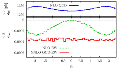
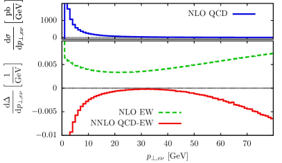
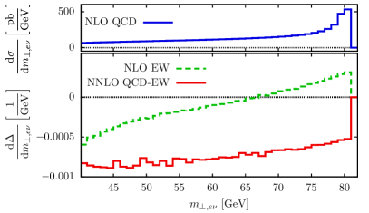
Figure 2: The impact of mixed QCD-electroweak corrections to $pp\to W^{+}(e^{+}\nu)$ production at $13\leavevmode\nobreak\ {\rm TeV}$ LHC on various kinematic distributions including lepton rapidity and transverse momentum, the transverse momentum of the $W$-boson and the transverse mass. NLO electroweak corrections are also shown. See text for details.

Since we do not aim at performing extensive phenomenological studies in this paper, we apply very mild cuts on the final state of the process $pp\to W^{+}(\bar{e}\nu)+X$. We require that the transverse momentum of the positron $p_{\perp,e}$ and of the neutrino $p_{\perp,\rm miss}$ are larger than $15\leavevmode\nobreak\ {\rm GeV}$ and that the absolute value of the positron rapidity does not exceed $|y_{e}|<2.4$. We also set the factorization and renormalization scales to be equal $\mu_{R}=\mu_{F}=\mu$ and choose $\mu=M_{W}/2$ as the central scale for our computations.

To present the results, we write the fiducial cross section as

$$\sigma_{pp\to W^{+}}=\sigma_{\rm LO}+\Delta\sigma_{\rm NLO,\alpha_{s}}+\Delta\sigma_{\rm NLO,\alpha},+\Delta\sigma_{\rm NNLO,\alpha\alpha_{s}}+....$$ (130)

where the first term on the right hand side is the leading order cross section, the second term is the NLO QCD contribution, the third term is the NLO electroweak contribution and the last one is the mixed QCD-electroweak contribution. Ellipses in Eq.(130) stand for other contributions to the cross section, e.g. NNLO QCD ones.

We show the fiducial cross sections $pp\to W+X$, using the cuts described above, in Table 1. It follows from this table that NLO electroweak contributions are tiny – they modify the leading order cross section by just about $-0.02$ percent. For comparison, we note that NNLO QCD corrections are of the order of a few percent. We note that the smallness of these corrections is partially related to our choice of the $G_{\mu}$ renormalization scheme which appears to reduce the impact of electroweak corrections significantly. Although quite small as well, mixed QCD-electroweak corrections turn out to be larger than the NLO electroweak ones, at least for the setup considered here.

The relative importance of mixed QCD-electroweak corrections, at least compared to NLO electroweak corrections, is also apparent from the kinematic distributions shown in Fig. 2. These distributions are computed with the fiducial cuts described above; results shown in Fig. 2 are obtained for $\mu=M_{W}/2$. The $y$-axes in the lower panes correspond to bin-by-bin ratios of NLO electroweak and mixed QCD-electroweak contributions to NLO QCD cross sections

$${\rm d}\Delta_{i}=\frac{{\rm d}\Delta\sigma_{i}}{{\rm d}\sigma_{\rm LO}+{\rm d}\Delta\sigma_{\rm NLO,\alpha_{s}}}.$$ (131)

In Fig. 2 we show the rapidity and transverse momentum distributions of the charged lepton as well as the transverse mass and the transverse momentum distributions of the $W$ boson. It follows from Fig. 2 that mixed QCD-electroweak corrections are often larger than NLO electroweak ones and that the two types of corrections often have different shapes. It remains to be seen how these small effects impact the extraction of the $W$-boson mass from LHC data; we will investigate this important question in a separate publication.

VIII Conclusions

A better understanding of mixed QCD-electroweak corrections to $W$-boson production in hadron collisions is important for the precision electroweak physics program at the LHC. The calculation of these corrections is complicated by the fact that they require two- and one-loop virtual corrections with several internal and external masses as well as control on infra-red and collinear singularities that appear when photons and partons are radiated.

However, thanks to recent progress in developing subtraction schemes for QCD computations at the LHC and in technology for multi-loop computations, the calculation of mixed QCD-electroweak corrections to on-shell vector-boson production becomes relatively straightforward. To demonstrate this, in this paper we have presented results for the two-loop QCD-EW corrections to the $q\bar{q}^{\prime}\to W$ interaction vertex and explained how to construct a suitable subtraction scheme for real-emission contributions. We provided relatively simple analytic results for fully- and partially-unresolved integrated subtraction terms as well as analytic formulas and a numerical value for the two-loop form factor that describes mixed QCD-electroweak contributions to the $q\bar{q}^{\prime}\to W$ on-shell interaction vertex.

We have implemented our calculation in a flexible parton-level numerical code and used it to calculate mixed QCD-electroweak corrections to $pp\to W^{+}(e^{+}\nu)$ at the LHC. We presented results for fiducial cross sections and selected kinematic distributions. In the setup that we have considered, we have found that, in general, mixed QCD-electroweak corrections are rather small, often below a permille. However they appear to be larger than one-loop electroweak corrections to $pp\to W^{+}$ at least when the latter are computed in the $G_{\mu}$ scheme.

The calculation reported in this paper provides one of the last missing theoretical ingredients whose understanding is considered to be essential for achieving few MeV accuracy in the $W$-boson mass measurement at the LHC. Needless to say that the actual impact of these corrections on the $W$-mass measurement is unknown; we plan to study this question in a future publication.

Acknowledgment This research is partially supported by BMBF grant 05H18VKCC1 and by the Deutsche Forschungsgemeinschaft (DFG, German Research Foundation) under grant 396021762 - TRR 257. The research of F.B. and F.C. was partially supported by the ERC Starting Grant 804394 HipQCD.

Appendix A Infra-red structure of loop corrections

The computation of mixed QCD-EW corrections to $u\bar{d}\to W^{+}$ requires virtual corrections to a number of processes including i) two-loop mixed QCD-EW corrections to $u\bar{d}\to W^{+}$, ii) one-loop QCD corrections to $u\bar{d}\to W^{+}$, iii) one-loop electroweak corrections to $u\bar{d}\to W^{+}$, iv) one-loop QCD corrections to $u\bar{d}\to W^{+}+\gamma$, v) one-loop electroweak corrections to $u\bar{d}\to W^{+}+g$ as well as crossings of these processes. To demonstrate the cancellation of $1/\epsilon$ poles and identify the $\epsilon\to 0$ limit of the integrated subtraction terms, we need to isolate infra-red divergent contributions to these amplitudes. In case of QCD corrections, this can be accomplished with the help of Catani’s formula Catani:1998bh . In this appendix, we use the results of Ref. Catani:1998bh to explicitly extract the infra-red part of renormalized QCD amplitudes, and generalize them to deal with the electroweak case as well.

We use the following notation. We write a generic (renormalized) amplitude as

$$\mathcal{A}=\mathcal{A}_{0}+\left(\frac{\alpha_{s}(\mu)}{2\pi}\right)\mathcal{A}_{1}+\left(\frac{\alpha_{EW}}{2\pi}\right)\bar{\mathcal{A}}_{1}+\left(\frac{\alpha_{s}(\mu)}{2\pi}\;\frac{\alpha_{EW}}{2\pi}\right)\mathcal{A}_{\rm mix}+...$$ (132)

and then define

$$\begin{split}F_{\rm LV}^{\rm QCD}(1,2;...)&=\mathcal{N}\left(\frac{\alpha_{s}(\mu)}{2\pi}\right)\int\sum_{\rm col,pol}2\Re\big{[}\mathcal{A}_{0}\mathcal{A}_{1}^{*}\big{]}(2\pi)^{d}\delta_{d}(P_{i}-P_{f})\frac{\mathrm{d}^{d-1}p_{W}}{(2\pi)^{d-1}2E_{W}},\\ F_{\rm LV}^{\rm EW}(1,2;...)&=\mathcal{N}\left(\frac{\alpha_{EW}}{2\pi}\right)\int\sum_{\rm col,pol}2\Re\big{[}\mathcal{A}_{0}\bar{\mathcal{A}^{*}_{1}}\big{]}(2\pi)^{d}\delta_{d}(P_{i}-P_{f})\frac{\mathrm{d}^{d-1}p_{W}}{(2\pi)^{d-1}2E_{W}},\\ F_{{\rm LVV}+{\rm LV}^{2}}^{{\rm QCD}\otimes\rm{EW}}(1,2)&=\mathcal{N}\left(\frac{\alpha_{s}(\mu)}{2\pi}\;\frac{\alpha_{EW}}{2\pi}\right)\int\sum_{\rm col,pol}2\Re\big{[}\mathcal{A}_{0}\mathcal{A}_{2}^{*}+\mathcal{A}_{1}\bar{\mathcal{A}_{1}^{*}}\big{]}(2\pi)^{d}\delta_{d}(P_{i}-P_{f})\frac{\mathrm{d}^{d-1}p_{W}}{(2\pi)^{d-1}2E_{W}},\end{split}$$ (133)

where $P_{i(f)}$ stands for the sum of initial(final) momenta and $\mathcal{N}$ stands for all the required ($d$-dimensional) initial-state color and helicity averaging factors, see Eq.(1) and Refs. Caola:2017dug ; Caola:2019nzf . In this appendix, we also use the notation

$$\bar{\alpha}=\left[(4\pi)^{\epsilon}e^{-\epsilon\gamma_{E}}\right]\alpha_{EW}.$$ (134)

Formulas provided in this appendix are used in the main text to construct subtraction terms for mixed QCD-EW corrections and to demonstrate cancellation of $1/\epsilon$ singularities analytically.

A.1 The infra-red structure of real-virtual amplitudes

We begin with QCD corrections to the electroweak processes $u+\bar{d}\to W+\gamma$. The infra-red and collinear structure of the one-loop amplitude directly follows from Catani’s formula Catani:1998bh . We write

$$\begin{split}\left\langle F^{\rm QCD}_{\rm LV}(1_{u},2_{\bar{d}};4_{\gamma})\right\rangle&=\left(\frac{\alpha_{s}(\mu)}{2\pi}\right)\left[\frac{e^{\epsilon\gamma_{E}}}{\Gamma(1-\epsilon)}\right]\left(\frac{\mu^{2}}{s_{12}}\right)^{\epsilon}\left[-2C_{F}\cos(\pi\epsilon)\left(\frac{1}{\epsilon^{2}}+\frac{3}{2\epsilon}\right)\right]\langle F_{\rm LM}(1_{u},2_{\bar{d}};4_{\gamma})\rangle\\ &+\left\langle F_{\rm LV}^{\rm fin,QCD}(1_{u},2_{\bar{d}};4_{\gamma})\right\rangle,\end{split}$$ (135)

where $s_{12}=2p_{1}\cdot p_{2}$. The required formula for QCD corrections to the photon-quark collision process reads

$$\begin{split}\left\langle F^{\rm QCD}_{\rm LV}(1_{\gamma},2_{\bar{d}}\;;4_{\bar{u}})\right\rangle&=\left(\frac{\alpha_{s}(\mu)}{2\pi}\right)\left[\frac{e^{\epsilon\gamma_{E}}}{\Gamma(1-\epsilon)}\right]\left(\frac{\mu^{2}}{s_{24}}\right)^{\epsilon}\left[-2C_{F}\left(\frac{1}{\epsilon^{2}}+\frac{3}{2\epsilon}\right)\right]\langle F_{\rm LM}(1_{\gamma},2_{\bar{d}}\;;4_{\bar{u}})\rangle\\ &+\left\langle F_{\rm LV}^{\rm fin,QCD}(1_{\gamma},2_{\bar{d}}\;;4_{\bar{u}})\right\rangle,\end{split}$$ (136)

with $s_{24}=2p_{2}\cdot p_{4}$.

We also require one-loop electroweak corrections to the process $u+\bar{d}\to W^{+}+g$. We parametrize them in the following way

$$\begin{split}\left\langle F^{\rm EW}_{\rm LV}(1_{u},2_{\bar{d}};4_{g})\right\rangle&=\left(\frac{\bar{\alpha}}{2\pi}\right)\left[\frac{e^{\epsilon\gamma_{E}}}{\Gamma(1-\epsilon)}\right]\left(\frac{\mu^{2}}{M_{W}^{2}}\right)^{\epsilon}\big{[}-Q_{u}Q_{d}f_{1}-Q_{u}Q_{W}f_{2}+Q_{d}Q_{W}f_{3}\big{]}\langle F_{\rm LM}(1_{u},2_{\bar{d}};4_{g})\rangle\\ &+\left\langle F_{\rm LV}^{\rm fin,EW}(1_{u},2_{\bar{d}};4_{g})\right\rangle,\end{split}$$ (137)

where $Q_{W}=Q_{u}-Q_{d}$ and

$$\begin{split}&f_{1}=\frac{2}{\epsilon^{2}}+\frac{3-2L_{s}}{\epsilon}-3L_{s}+L_{s}^{2}-\pi^{2},\\ &f_{2}=\frac{1}{\epsilon^{2}}+\frac{5/2-2L_{t}}{\epsilon}-\frac{3}{2}L_{t}+L_{t}^{2},\\ &f_{3}=\frac{1}{\epsilon^{2}}+\frac{5/2-2L_{u}}{\epsilon}-\frac{3}{2}L_{u}+L_{u}^{2},\end{split}$$ (138)

with $L_{s}=\ln(s/M_{W}^{2})$, $L_{t}=\ln(1-t/M_{W}^{2})$, $L_{u}=\ln(1-u/M_{W}^{2})$. The Mandelstam invariants are defined as

$$s=(p_{1}+p_{2})^{2},\;\;\;\;t=(p_{1}-p_{W})^{2},\;\;\;\;u=(p_{2}-p_{W})^{2}.$$ (139)

A related quantity is the one-loop electroweak corrections to the gluon-initiated process $g+\bar{d}\to W^{+}+\bar{u}$. We parametrize it in the following way

$$\begin{split}\left\langle F^{\rm EW}_{\rm LV}(1_{g},2_{\bar{d}};4_{\bar{u}})\right\rangle&=\left(\frac{\bar{\alpha}}{2\pi}\right)\left[\frac{e^{\epsilon\gamma_{E}}}{\Gamma(1-\epsilon)}\right]\left(\frac{\mu^{2}}{M_{W}^{2}}\right)^{\epsilon}\big{[}-Q_{u}Q_{d}f^{gq}_{1}-Q_{u}Q_{W}f^{gq}_{2}+Q_{d}Q_{W}f^{gq}_{3}\big{]}\langle F_{\rm LM}(1_{g},2_{\bar{d}};4_{\bar{u}})\rangle\\ &+\left\langle F_{\rm LV}^{\rm fin,EW}(1_{g},2_{\bar{d}},4_{\bar{u}})\right\rangle,\end{split}$$ (140)

where $Q_{W}=Q_{u}-Q_{d}$ and

$$\begin{split}&f^{gq}_{1}=\frac{2}{\epsilon^{2}}+\frac{3-2L_{24}}{\epsilon}-3L_{24}+L_{24}^{2},\\ &f^{gq}_{2}=\frac{1}{\epsilon^{2}}+\frac{5/2-2L_{4W}}{\epsilon}-\frac{3}{2}L_{4W}+L_{4W}^{2}-\pi^{2},\\ &f_{3}^{gq}=\frac{1}{\epsilon^{2}}+\frac{5/2-2L_{2W}}{\epsilon}-\frac{3}{2}L_{2W}+L_{2W}^{2},\end{split}$$ (141)

with $L_{24}=\ln(2p_{2}\cdot p_{4}/M_{W}^{2})$, $L_{4W}=\ln(2p_{4}\cdot p_{W}/M_{W}^{2})$, $L_{2W}=\ln(2p_{2}\cdot p_{W}/M_{W}^{2})$.

In all the formulas above, the infra-red $1/\epsilon$ poles are explicitly extracted and $F_{\rm LV}^{\rm fin,QCD/EW}$ are finite remainders.

A.2 Infra-red structure of the $Wq\bar{q}^{\prime}$ form factor

The only two-loop amplitude that we require describes mixed QCD-EW corrections to the $q+\bar{q}^{\prime}\to W^{+}$ process. For definiteness, we present results for the $u+\bar{d}\to W^{+}$ channel.

At one-loop, we parametrize QCD corrections as

$$\begin{split}&\left\langle F_{\rm LV}^{\rm QCD}(1_{u},2_{\bar{d}})\right\rangle=\left(\frac{\alpha_{s}(\mu)}{2\pi}\right)I_{12,{\rm QCD}}\left\langle F_{\rm LM}(1_{u},2_{\bar{d}})\right\rangle+\left\langle F_{\rm LM}^{\rm fin,QCD}(1_{u},2_{\bar{d}})\right\rangle,\\ &\left\langle F_{\rm LV}^{\rm EW}(1_{u},2_{\bar{d}})\right\rangle=\left(\frac{\bar{\alpha}}{2\pi}\right)I_{12,{\rm EW}}\left\langle F_{\rm LM}(1_{u},2_{\bar{d}})\right\rangle+\left\langle F_{\rm LM}^{\rm fin,EW}(1_{u},2_{\bar{d}})\right\rangle,\end{split}$$ (142)

with

$$\begin{split}&I_{12,\rm QCD}=\left[\frac{e^{\epsilon\gamma_{E}}}{\Gamma(1-\epsilon)}\right]\left(\frac{\mu^{2}}{M_{W}^{2}}\right)^{\epsilon}\left[-2C_{F}\cos(\pi\epsilon)\left(\frac{1}{\epsilon^{2}}+\frac{3}{2\epsilon}\right)\right],\\ &I_{12,\rm EW}=\left[\frac{e^{\epsilon\gamma_{E}}}{\Gamma(1-\epsilon)}\right]\left(\frac{\mu^{2}}{M_{W}^{2}}\right)^{\epsilon}\big{[}-Q_{u}Q_{d}\bar{f}_{1}-Q_{u}Q_{W}\bar{f}_{2}+Q_{d}Q_{W}\bar{f}_{3}\big{]},\end{split}$$ (143)

and

$$\bar{f}_{1}=\cos(\pi\epsilon)\left[\frac{2}{\epsilon^{2}}+\frac{3}{\epsilon}\right],\leavevmode\nobreak\ \leavevmode\nobreak\ \leavevmode\nobreak\ \bar{f}_{2}=\bar{f}_{3}=\frac{1}{\epsilon^{2}}+\frac{5}{2\epsilon}.$$ (144)

We note that these formulas agree with the $s\to M_{W}^{2}$, $t,u\to 0$ limit of Eqs.(135,137).

We now discuss the infra-red structure of two-loop mixed QCD-EW corrections. As we have explained in the main text, IR singularities in this case almost factorize into the product of two NLO-like structures. The only exceptions are genuinely-NNLO hard triple-collinear configurations. As a consequence, we can write

$$\begin{split}\left\langle F_{{\rm LVV}+{\rm LV}^{2}}^{{\rm QCD}\otimes{\rm EW}}(1_{u},2_{\bar{d}})\right\rangle&=\left(\frac{\alpha_{s}(\mu)}{2\pi}\;\frac{\bar{\alpha}}{2\pi}\right)\left[I_{12,\rm QCD}\cdot I_{12,\rm EW}+\frac{e^{\epsilon\gamma_{E}}}{\Gamma(1-\epsilon)}\frac{H^{W}_{{\rm QCD}\otimes{\rm EW}}}{\epsilon}\right]\left\langle F_{LM}(1_{u},2_{\bar{d}})\right\rangle\\ &+\left(\frac{\alpha_{s}(\mu)}{2\pi}\right)I_{12,\rm QCD}\left\langle F_{\rm LV}^{\rm fin,EW}(1_{u},2_{\bar{d}})\right\rangle+\left(\frac{\bar{\alpha}}{2\pi}\right)I_{12,\rm EW}\left\langle F_{\rm LV}^{\rm fin,QCD}(1_{u},2_{\bar{d}})\right\rangle\\ &+\left\langle F_{{\rm LVV}+{\rm LV}^{2}}^{{\rm fin,QCD}\otimes{\rm EW}}(1_{u},2_{\bar{d}})\right\rangle.\end{split}$$ (145)

In Eq.(145), $F_{{\rm LVV}+{\rm LV}^{2}}^{{\rm fin,QCD}\otimes{\rm EW}}$ is the two-loop finite remainder. The constant $H^{W}_{{\rm QCD}\otimes{\rm EW}}$ is related to the quark anomalous dimension and can be extracted by abelianizing the corresponding contribution in Ref. Catani:1998bh . It reads

$$H^{W}_{{\rm QCD}\otimes{\rm EW}}=\left(\frac{\pi^{2}}{2}-6\zeta_{3}-\frac{3}{8}\right)C_{F}\big{[}Q_{u}^{2}+Q_{d}^{2}\big{]}.$$ (146)

We present explicit formulas for the one- and two-loop finite remainders in the next appendix.

Appendix B Analytic expression for the mixed QCD-EW form factor

The double-virtual corrections to single on-shell $W$-boson production require the form factor for the $q\bar{q}^{\prime}\to W$ vertex at $\mathcal{O}(\alpha_{s}\alpha_{EW})$. The on-shell condition simplifies the problem significantly; in particular, we do not need complicated two-loop four-point functions Bonciani:2016ypc ; vonManteuffel:2017myy ; Heller:2019gkq ; Hasan:2020vwn required to describe the process $pp\to l\nu$ with ${\cal O}(\alpha_{s}\alpha_{EW})$ accuracy in the off-shell case. Moreover, if one assumes equal masses for internal $W$ and $Z$ bosons, all necessary integrals are available in the literature and can be extracted from Refs. Aglietti:2003yc ; Aglietti:2004tq ; Bonciani:2016ypc ; vonManteuffel:2017myy ; Heller:2019gkq ; Hasan:2020vwn . However, to the best of our knowledge, results for on-shell $W$ form factor that accommodate different masses of $W$ and $Z$ bosons are not publicly available. We compute the relevant form factor in this paper.

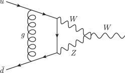
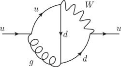
Figure 3: Examples for mixed QCD-electroweak two-loop diagrams. A form factor diagram with simultaneous internal $W$- and $Z$-boson propagators is shown on the left. A self-energy diagram which contributes to the wave function renormalization of the external quarks at $\mathcal{O}(\alpha_{s}\alpha_{EW})$ is shown on the right.

An example of a diagram that has to be computed is shown in Fig. 3. In order to calculate the form factor, we use QGRAF Nogueira:1991ex to generate diagrams, FORM Vermaseren:2000nd ; Kuipers:2012rf ; Kuipers:2013pba ; Ruijl:2017dtg to perform the Dirac and Lorentz algebra, color.h vanRitbergen:1998pn for the color algebra and Reduze2 vonManteuffel:2012np ; Bauer:2000cp ; Lewis:Fermat to reduce integrals that appear to master integrals using integration-by-parts relations Chetyrkin:1980pr ; Chetyrkin:1981qh ; Tkachov:1981wb . We work in the Feynman gauge and use Feynman rules from Ref. Bohm:2001yx . Since we only require contributions of massless quarks and work at $\mathcal{O}(\alpha_{s}\alpha_{EW})$, the Dirac matrix $\gamma_{5}$ can only appear on fermion lines that are connected to external lines. For this reason, we consider $\gamma_{5}$ to be anti-commuting.

The form factor has to be renormalized in order to remove ultra-violet divergences. We choose to follow the procedure described in Ref. Denner:1991kt and renormalize the wave functions and masses in the on-shell scheme. We use the $\overline{\text{MS}}$ scheme to renormalize the strong coupling constant $\alpha_{s}$ and the $G_{\mu}$ scheme for the electroweak input parameters. The weak mixing angle is defined as $\cos\theta_{W}=M_{W}/M_{Z}$ in terms of the on-shell $W$ and $Z$ boson masses. The necessary renormalization constants at the one-loop order are given explicitly in Ref. Denner:1991kt . The two-loop mixed QCD-electroweak corrections to the self-energies of electroweak gauge bosons were calculated in Ref. Djouadi:1993ss . In addition, we need the two-loop self-energies for massless fermions which enters through the wave function renormalization of external quarks. A typical diagram that appears in this context is the self-energy diagram shown in Fig. 3. The required wave function renormalization has already been calculated in Ref. Buccioni:2020cfi ; it reads

$$Z_{f,L}={} 1-\left(\frac{\alpha}{2\pi}\frac{(4\pi)^{\epsilon}}{\mu^{\epsilon}}\right)\frac{1-\epsilon}{(2-\epsilon)\epsilon}\Gamma(1+\epsilon)\left(g_{f,L}^{2}\left(\frac{M_{Z}^{2}}{\mu^{2}}\right)^{-\epsilon}+\frac{1}{2\sin^{2}(\theta_{W})}\left(\frac{M_{W}^{2}}{\mu^{2}}\right)^{-\epsilon}\right)$$

$$+\left(\frac{\alpha}{2\pi}\frac{\alpha_{s}}{2\pi}\frac{(4\pi)^{2\epsilon}}{\mu^{2\epsilon}}\right)C_{F}\frac{(3-2\epsilon)(1-3\epsilon)}{4\epsilon(2-\epsilon)(1-2\epsilon)}\Gamma(1-\epsilon)\Gamma(1+\epsilon)\Gamma(1+2\epsilon)$$ (147)

$$\hphantom{+\leavevmode\nobreak\ }\times\left(g_{f,L}^{2}\left(\frac{M_{Z}^{2}}{\mu^{2}}\right)^{-2\epsilon}+\frac{1}{2\sin^{2}(\theta_{W})}\left(\frac{M_{W}^{2}}{\mu^{2}}\right)^{-2\epsilon}\right)\,.$$

The bare strong and electromagnetic coupling constants are $\alpha_{s}$ and $\alpha$, respectively, and the subscript $f\in\{u,d\}$ denotes the type of fermion. The $Z$-boson coupling is defined as

$$g_{f,L} =\frac{I_{3,f}-Q_{f}\sin^{2}(\theta_{W})}{\sin(\theta_{W})\cos(\theta_{W})},$$ (148)

where $I_{3,f}=\pm 1/2$ and $Q_{f}$ are the third component of the weak isospin and the electric charge of the fermion $f$. We have checked the renormalization constants by rederiving them using the same set of programs as described above. We have also checked the renormalization constants related to vector bosons by comparing numerically against results of Ref. ditt2 .

We note that the one-loop renormalization constants also enter the two-loop renormalization where they are multiplied by infra-red divergent quantities. Therefore, one would a priori also need higher-order terms beyond $\mathcal{O}(\epsilon^{0})$ for these renormalization constants. However, once one-loop squared and genuine two-loop contributions are combined, the higher-order terms cancel out and so there is no need to compute them.

To check the correctness of our result, we performed two independent calculations and found agreement. We have also checked that the $1/\epsilon$ infra-red poles of the renormalized form-factor agree with the general structure discussed in the previous appendix.

We now discuss some details of the calculation. After IBP reduction, we find ten master integrals with two different internal masses. We compute them using differential equations Kotikov:1990kg ; Caffo:1998du ; Gehrmann:1999as . The integration constants are fixed by matching to the known results in the equal mass limit which we take from Refs. Aglietti:2003yc ; Aglietti:2004tq ; Bonciani:2016ypc . To verify the computed master integrals, we have numerically checked our results using pySecDec Borowka:2017idc ; Borowka:2018goh ; Vermaseren:2000nd ; Kuipers:2012rf ; Kuipers:2013pba ; Ruijl:2017dtg ; Hahn:2004fe ; Hahn:2014fua ; GSL .

To write down the differential equations that the master integrals satisfy, we find it convenient to rationalize the square root present in the alphabet by introducing the standard Landau variable $y$ defined as follows

$$\frac{M_{Z}^{2}}{M_{W}^{2}} =\frac{(1+y)^{2}}{y}.$$ (149)

When written in this variable, the differential equation for the vector of master integrals $I$ can be written as

$$\partial_{y}\vec{I} =\sum\limits_{a\in S}\sum_{k=0}^{5}\frac{\hat{A}_{a,k}}{(y-a)^{k}}\vec{I},$$ (150)

where

$$S=\left\{0,\pm 1,\pm i,e^{\pm\frac{2i\pi}{3}},-\varphi^{2},-\varphi^{-2}\right\}\,,$$ (151)

and $\varphi=\frac{1+\sqrt{5}}{2}$ is the golden ratio.

The differential equation Eq.(150) is solved in terms of Goncharov Polylogarithms (GPLs). Manipulations of GPLs were done using different tools, including HarmonicSums Ablinger:2010kw ; Ablinger:2013hcp ; Vermaseren:1998uu ; Remiddi:1999ew ; Blumlein:2009ta ; Ablinger:2011te ; Ablinger:2013cf ; Ablinger:2014rba ; Ablinger:2016ll ; Ablinger:2017rad ; Ablinger:2019mkx and PolyLogTools Maitre:2005uu ; Maitre:2007kp ; Duhr:2019tlz . We have simplified GPLs that appear in the calculation using relations from Refs. Henn:2015sem ; Ablinger:2011te . In the solutions of the master integrals the letters $a=\pm i$ no longer appear. Although the result expressed in terms of the $y$ variable is straightforward to evaluate, its analytic form is somewhat unwieldy. Because of this, we decided to present our analytic result expressed in terms of

$$z=\frac{M_{W}^{2}}{M_{Z}^{2}}+i0.$$ (152)

Results in terms of $y$ can be obtained from the authors upon request.

We express our results in terms of iterated integrals defined as

$$H_{\underbrace{0,\dots,0}_{k\text{ times}}}(z) =\frac{1}{k!}\ln^{k}(z)\,, H_{a}(z) =\int_{0}^{z}\mathrm{d}x\,f_{a}(x)\,, H_{a_{1},\dots,a_{n}}(z) =\int_{0}^{z}\mathrm{d}x\,f_{a_{1}}(x)H_{a_{2},\dots,a_{m}}(x)$$ (153)

with the alphabet

$$f_{0}(x) =\frac{1}{x}\,, f_{1}(x) =\frac{1}{1-x}\,, f_{-1}(x) =\frac{1}{1+x}\,, f_{r}(x) =\frac{1}{\sqrt{x(4-x)}}\,.$$ (154)

We also find it convenient to define the following combinations

$$\mathcal{H}_{1} =H_{r}({z^{-1}})-\pi\,,$$

$$\mathcal{H}_{2} =\pi H_{0}({z})+H_{0,r}({z^{-1}})\,,$$

$$\mathcal{H}_{3} =i\pi^{2}-3i\pi H_{r}({z^{-1}})-3H_{r,1}({z^{-1}})\,,$$

$$\mathcal{H}_{4} =H_{r,0}({z^{-1}})\,,$$

$$\mathcal{H}_{5} =-\pi H_{r}({z^{-1}})+H_{r,r}({z^{-1}})\,,$$ (155)

$$\mathcal{H}_{6} =-\pi H_{0,r}({z^{-1}})+H_{0,r,r}({z^{-1}})\,,$$

$$\mathcal{H}_{7} =-\pi H_{r,0}({z^{-1}})+H_{r,0,r}({z^{-1}})\,,$$

$$\mathcal{H}_{8} =H_{r,r,0}({z^{-1}})\,,$$

$$\mathcal{H}_{9} =-i\frac{\pi^{3}}{6}+i\pi^{2}H_{r}({z^{-1}})-3i\pi H_{r,r}({z^{-1}})-3H_{r,r,1}({z^{-1}})\,,$$

$$\mathcal{H}_{10} =i\frac{\pi^{3}}{6}H_{0}({z})+i\pi^{2}H_{0,r}({z^{-1}})-3i\pi H_{0,r,r}({z^{-1}})-3H_{0,r,r,0}({z^{-1}})-3H_{0,r,r,1}({z^{-1}})-4i\pi\zeta_{3}\,.$$

These combinations evaluate to real numbers in the relevant physical region $M_{W}^{2}\leq M_{Z}^{2}$, i.e. $0\leq z\leq 1$. However, note that the iterated integrals where the square-root-valued letter $f_{r}$ occurs are evaluated at argument $z^{-1}\geq 1$. Therefore, the individual iterated integrals with simultaneous letters $f_{r}$ and $f_{1}$ develop an imaginary part that cancels against the explicit imaginary parts in $\mathcal{H}_{3}$, $\mathcal{H}_{9}$ and $\mathcal{H}_{10}$.

We now present our results. For completeness, we first report expressions for one-loop corrections. We write the finite remainders defined in Appendix A as

$$\left\langle F_{\rm LV}^{\rm fin,QCD}(1_{u},2_{\bar{d}})\right\rangle=\left(\frac{\alpha_{s}(\mu)}{2\pi}\right)\mathcal{F}_{u\bar{d}}^{\rm QCD,fin}\left\langle F_{\rm LM}(1_{u},2_{\bar{d}})\right\rangle,\leavevmode\nobreak\ \left\langle F_{\rm LV}^{\rm fin,EW}(1_{u},2_{\bar{d}})\right\rangle=\left(\frac{\alpha_{EW}}{2\pi}\right)\mathcal{F}_{u\bar{d}}^{\rm EW,fin}\left\langle F_{\rm LM}(1_{u},2_{\bar{d}})\right\rangle.$$ (156)

With this notation, the (renormalized) form factors read $\mathcal{F}_{u\bar{d}}^{\rm QCD,fin}=-8C_{F},$ and

$$\mathcal{F}_{u\bar{d}}^{\rm EW,fin}={}(Q_{u}^{2}+Q_{d}^{2})\Biggl{[}\frac{\big{(}z-1\big{)}(1+z)^{2}}{z^{3}}H_{-1,0}({z})-\frac{1}{2}\frac{\big{(}z-1\big{)}\big{(}3z+2\big{)}}{z^{2}}H_{0}({z})-\frac{1}{4}\frac{9z^{2}+3z+4}{z^{2}}\Biggr{]}$$

$$+N_{c}\Biggl{[}\frac{1}{4}\frac{\big{(}z_{t}-1\big{)}\big{(}z_{t}+1\big{)}}{\big{(}z-1\big{)}z_{t}^{3}}H_{1}({z_{t}})-\frac{1}{8}\frac{4z_{t}^{2}-z_{t}-2}{\big{(}z-1\big{)}z_{t}^{2}}\Biggr{]}-\frac{1}{2}\frac{\big{(}2z^{2}-2z+1\big{)}(1+z)^{2}}{\big{(}z-1\big{)}z^{3}}H_{-1,0}({z})$$

$$+\frac{1}{16}\frac{4z_{H}^{4}-22z_{H}^{3}+17z_{H}^{2}-6z_{H}+1}{\big{(}z-1\big{)}\big{(}z_{H}-1\big{)}z_{H}^{3}}H_{0}({z_{H}})-\frac{1}{16}\frac{16z^{5}+20z^{4}-118z^{3}+79z^{2}-2z-1}{\big{(}z-1\big{)}^{2}z^{3}}H_{0}({z})$$ (157)

$$+\frac{1}{48}\frac{-6z^{2}+21z^{2}z_{H}-30z_{H}^{2}-69zz_{H}^{2}+418z^{2}z_{H}^{2}}{\big{(}z-1\big{)}z^{2}z_{H}^{2}}+\frac{1}{6}\frac{2z+7}{z-1}\pi^{2}+\frac{z+2}{z-1}\Bigl{(}H_{0,0}({z})+\mathcal{H}_{5}(z)\Bigr{)}$$

$$-\frac{\sqrt{4z_{H}-1}}{z_{H}}\frac{1}{16}\frac{28z_{H}^{3}-20z_{H}^{2}+7z_{H}-1}{\big{(}z-1\big{)}\big{(}4z_{H}-1\big{)}z_{H}^{2}}\mathcal{H}_{1}(z_{H})+\frac{\sqrt{4z-1}}{z}\frac{1}{16}\frac{28z^{3}+52z^{2}-13z-1}{\big{(}z-1\big{)}z^{2}}\mathcal{H}_{1}(z).$$

In Eq.(157), we used

$$z =\frac{M_{W}^{2}}{M_{Z}^{2}}+i0\,, z_{H} =\frac{M_{W}^{2}}{M_{H}^{2}}+i0\,, z_{t} =\frac{M_{W}^{2}}{M_{t}^{2}}+i0\,.$$ (158)

We now present results for the mixed QCD-EW corrections. We find it convenient to factor out the LO amplitude and separate factorizable and non-factorizable contributions. We write

$$\mathcal{A}_{\rm mix}=\mathcal{A}_{0}\left[\mathcal{M}_{1}\bar{\mathcal{M}}_{1}+\mathcal{M}_{\rm mix,n.f.}\right],$$ (159)

where $\mathcal{A}_{i}$ are defined in Eq.(132) and we used analogous definitions for $\mathcal{M}_{i}$. Following what was done in Ref. kkv for the $Z$ boson, we also separate the renormalization contribution coming from two-loop gauge-bosons self-energy corrections, which is finite. We then write

$$\mathcal{M}_{\rm mix,n.f.}=\widetilde{\mathcal{M}}_{\rm mix}+\delta Z_{{\rm mix},2},\leavevmode\nobreak\ \leavevmode\nobreak\ \leavevmode\nobreak\ \leavevmode\nobreak\ \widetilde{\mathcal{M}}_{\rm mix}=\mathcal{M}_{\rm mix,bare}+\delta Z_{{\rm mix},1},$$ (160)

where $\delta Z_{{\rm mix},1}$ contains the mixed fermion wave-function renormalization Eq.(147) and $\delta Z_{{\rm mix},2}$ contains the remaining renormalization. In analogy with Ref. kkv , we now present results for $\widetilde{\mathcal{M}}_{\rm mix}$. We obtain

$$\widetilde{\mathcal{M}}_{\rm mix}={} \big{(}Q_{u}^{2}+Q_{d}^{2}\big{)}C_{F}\Biggl{[}\frac{1}{\epsilon}\biggl{(}-\frac{3}{16}+\frac{1}{4}\pi^{2}-3\zeta_{3}\biggr{)}+\biggl{(}\frac{3}{8}-\frac{1}{2}\pi^{2}+6\zeta_{3}\biggr{)}\ln\left(\frac{M_{W}^{2}}{\mu^{2}}\right)+\frac{1}{4}\frac{\big{(}27z+13\big{)}(1-z)^{2}}{z^{3}}H_{1}$$

$$+\frac{(1-z)^{2}(1+z)}{z^{3}}\biggl{(}\frac{3}{4}H_{1}\pi^{2}-\frac{9}{2}H_{1,0,0}-\frac{9}{2}H_{1,0,1}\biggr{)}-\frac{1}{4}\frac{\big{(}5z+3\big{)}(1-z)(1+z)}{z^{3}}H_{-1,0}$$

$$+\frac{(1-z)(1+z)^{2}}{z^{3}}\biggl{(}-\frac{3}{2}H_{-1,-1,0}+\frac{3}{2}H_{-1,0,0}+3H_{-1,0,1}+2H_{-1,-1,-1,0}-2H_{-1,-1,0,0}-6H_{-1,-1,0,1}$$

$$-2H_{-1,0,-1,0}+H_{-1,0,0,1}+H_{0,-1,0,0}+4H_{0,-1,0,1}+\Bigl{(}-\frac{1}{4}H_{-1}+\frac{1}{6}H_{-1,-1}-\frac{1}{6}H_{0,-1}\Bigr{)}\pi^{2}-3H_{-1}\zeta_{3}\biggr{)}$$

$$+\frac{1}{32}\frac{7z^{2}-72z+64}{z^{2}}+\frac{1}{24}\frac{50z^{2}-5z-16}{z^{2}}\pi^{2}-\frac{3}{2}\frac{8z^{2}-z-2}{z^{2}}\zeta_{3}-\frac{11}{180}\pi^{4}+\frac{(1-z)}{z^{2}}\biggl{(}\frac{1}{2}\big{(}9z+11\big{)}H_{0,1}$$

$$-\frac{1}{2}\big{(}3z+4\big{)}H_{0,0,1}+\big{(}3z+2\big{)}\Bigl{(}-\frac{17}{8}H_{0}+\frac{1}{2}H_{0,-1,0}\Bigr{)}+\frac{1}{4}\big{(}23z+16\big{)}H_{0,0}\biggr{)}$$

$$+\frac{\big{(}z^{2}+3z+1\big{)}(1-z)}{z^{3}}\biggl{(}\frac{1}{3}H_{0,1}\pi^{2}-2H_{0,1,0,0}-2H_{0,1,0,1}\biggr{)}\Biggr{]}$$

$$+C_{F}\Biggl{[}\frac{z+2}{1-z}\Bigl{(}-\frac{1}{6}H_{0,0}\pi^{2}+4H_{0}\zeta_{3}\Bigr{)}+\frac{1}{8}\frac{\big{(}5z-2\big{)}\big{(}2z^{2}+12z+11\big{)}}{(1-z)z^{2}}H_{0,1}+\frac{1}{8}\frac{43z^{2}+7z-16}{(1-z)z^{2}}H_{0,0}$$

$$-\frac{1}{16}\frac{8z^{3}+142z^{2}+23z-34}{(1-z)z^{2}}H_{0}-\frac{1}{48}\frac{10z^{3}+5z^{2}+20z-16}{(1-z)z^{2}}\pi^{2}+\frac{1}{120}\frac{5z-36}{1-z}\pi^{4}-\frac{1}{8}\frac{4z^{2}-17z+8}{(1-z)z^{2}}$$

$$+\frac{2z^{2}-2z+1}{(1-z)z^{2}}\biggl{(}\big{(}3z+2\big{)}\Bigl{(}-\frac{3}{4}\zeta_{3}-\frac{1}{4}H_{0,-1,0}\Bigr{)}+\frac{1}{4}\big{(}3z+4\big{)}H_{0,0,1}\biggr{)}+\frac{\big{(}2z^{2}-6z+3\big{)}(1+z)}{z^{3}}\biggl{(}\frac{3}{4}H_{1,0,0}$$

$$+\frac{3}{4}H_{1,0,1}-\frac{1}{8}H_{1}\pi^{2}\biggr{)}-\frac{1}{(1-z)z}\biggl{(}\frac{1}{8}H_{0,0,0}+\frac{1}{2}\big{(}9z^{2}-8z-2\big{)}\zeta_{3}+\frac{5}{48}H_{0}\pi^{2}\biggr{)}$$

$$+\frac{\big{(}2z^{2}-2z+1\big{)}(1+z)^{2}}{(1-z)z^{3}}\biggl{(}\frac{3}{4}H_{-1,-1,0}-\frac{3}{4}H_{-1,0,0}-\frac{3}{2}H_{-1,0,1}-H_{-1,-1,-1,0}+H_{-1,-1,0,0}+3H_{-1,-1,0,1}$$

$$+H_{-1,0,-1,0}-\frac{1}{2}H_{-1,0,0,1}-\frac{1}{2}H_{0,-1,0,0}-2H_{0,-1,0,1}+\Bigl{(}\frac{1}{8}H_{-1}-\frac{1}{12}H_{-1,-1}+\frac{1}{12}H_{0,-1}\Bigr{)}\pi^{2}+\frac{3}{2}H_{-1}\zeta_{3}\biggr{)}$$

$$+\frac{1}{8}\frac{4z^{3}+64z^{2}-z-13}{z^{3}}H_{1}+\frac{1}{8}\frac{\big{(}5z+3\big{)}\big{(}2z^{2}-2z+1\big{)}(1+z)}{(1-z)z^{3}}H_{-1,0}+\frac{z^{4}-4z^{2}+z+1}{(1-z)z^{3}}\biggl{(}H_{0,1,0,0}$$

$$+H_{0,1,0,1}-\frac{1}{6}H_{0,1}\pi^{2}\biggr{)}+\biggl{[}\frac{\sqrt{4z-1}}{z}\biggl{(}-\frac{1}{8}\frac{10z+3}{1-z}\mathcal{H}_{1}-\frac{1}{8}\mathcal{H}_{2}-\frac{1}{8}\frac{6z+1}{1-z}\mathcal{H}_{3}+\frac{1}{8}\frac{17z+4}{1-z}\mathcal{H}_{4}\biggr{)}$$

$$-\frac{1}{8}\frac{3z+2}{(1-z)z}\mathcal{H}_{5}+\frac{1}{8}\frac{1}{(1-z)z}\mathcal{H}_{6}-\frac{1}{8}\frac{6z^{2}-4z+1}{(1-z)z}\mathcal{H}_{7}-\frac{1}{8}\frac{30z^{2}-20z-1}{(1-z)z}\mathcal{H}_{8}+\frac{1}{2}\frac{3z-2}{1-z}\mathcal{H}_{9}+\frac{z+2}{1-z}\mathcal{H}_{10}\biggr{]}\Biggr{]}$$

$$+i\pi\Biggl{\{}\big{(}Q_{u}^{2}+Q_{d}^{2}\big{)}C_{F}\Biggl{[}\frac{9}{2}\frac{(1-z)^{2}(1+z)}{z^{3}}H_{1,0}+\frac{(1-z)(1+z)^{2}}{z^{3}}\biggl{(}\frac{3}{2}H_{-1,-1}-\frac{3}{2}H_{-1,0}-2H_{-1,-1,-1}$$

$$+2H_{-1,-1,0}+2H_{-1,0,-1}-H_{0,-1,0}\biggr{)}+\frac{(1-z)}{z^{2}}\biggl{(}-\frac{1}{2}\big{(}3z+2\big{)}H_{0,-1}-\frac{1}{4}\big{(}23z+16\big{)}H_{0}\biggr{)}$$

$$+\frac{1}{4}\frac{\big{(}5z+3\big{)}(1-z)(1+z)}{z^{3}}H_{-1}+\frac{\big{(}z^{2}+3z+1\big{)}(1-z)}{z^{3}}2H_{0,1,0}-\frac{1}{8}\frac{54z^{2}-17z-34}{z^{2}}+\frac{1}{2}\pi^{2}-6\zeta_{3}\Biggr{]}$$

$$+C_{F}\Biggl{[}\frac{1}{16}\frac{8z^{3}+372z^{2}+17z-34}{(1-z)z^{2}}-\frac{3}{4}\frac{\big{(}2z^{2}-6z+3\big{)}(1+z)}{z^{3}}H_{1,0}-\frac{1}{8}\frac{\big{(}2z-1\big{)}\big{(}23z+16\big{)}}{(1-z)z^{2}}H_{0}$$

$$+\frac{\big{(}2z^{2}-2z+1\big{)}(1+z)^{2}}{(1-z)z^{3}}\biggl{(}\frac{3}{4}H_{-1,0}-\frac{3}{4}H_{-1,-1}-H_{-1,-1,0}+H_{-1,-1,-1}-H_{-1,0,-1}+\frac{1}{2}H_{0,-1,0}\biggr{)}$$

$$+\frac{1}{4}\frac{\big{(}3z+2\big{)}\big{(}2z^{2}-2z+1\big{)}}{(1-z)z^{2}}H_{0,-1}-\frac{1}{8}\frac{\big{(}5z+3\big{)}\big{(}2z^{2}-2z+1\big{)}(1+z)}{(1-z)z^{3}}H_{-1}-\frac{z^{4}-4z^{2}+z+1}{(1-z)z^{3}}H_{0,1,0}$$

$$-\frac{1}{4}\pi^{2}-12\frac{1}{(1-z)}\zeta_{3}\Biggr{]}\Biggr{\}}\,.$$ (161)

In Eq. (161) we omit writing down the argument $z$ of the iterated integrals. Real and imaginary parts in Eq. (161) are explicitly separated.

For completeness, we also present results for the $\delta Z_{{\rm mix},2}$ term. We obtain

$$\delta Z_{{\rm mix},2}={}\frac{N_{c}C_{F}}{4(1-z)}\Biggl{\{}\frac{\big{(}z_{t}+1\big{)}(1-z_{t})}{z_{t}^{3}}\biggl{[}\frac{1}{6}H_{1}({z_{t}})\pi^{2}-H_{0,1,1}({z_{t}})+H_{1,0,1}({z_{t}})\biggr{]}+\frac{1}{12}\frac{\big{(}17z_{t}+15\big{)}(1-z_{t})}{z_{t}^{3}}H_{1}({z_{t}})$$

$$+\frac{1}{3}\frac{2z_{t}^{2}-3}{z_{t}^{2}}H_{0,1}({z_{t}})-\frac{1}{6}\frac{\big{(}4z_{t}^{2}-5z_{t}-17\big{)}(1-z_{t})}{z_{t}^{3}}H_{1,1}({z_{t}})+\frac{1}{36}\frac{4z_{t}^{2}-3z_{t}-6}{z_{t}^{2}}\pi^{2}+\frac{1}{24}\frac{36z_{t}^{2}-35z_{t}-30}{z_{t}^{2}}\Biggr{\}}.$$ (162)

Starting from the definitions Eqs.(159,160) it is straightforward to obtain the two-loop finite remainder $F_{{\rm LVV}+{\rm LV}^{2}}^{{\rm fin,QCD}\otimes{\rm EW}}$ Eq.(145). It reads

$$\begin{split}&\left\langle F_{{\rm LVV}+{\rm LV}^{2}}^{{\rm fin,QCD}\otimes{\rm EW}}(1_{u},2_{\bar{d}})\right\rangle={}\left(\frac{\alpha_{s}(\mu)}{2\pi}\;\frac{\alpha_{EW}}{2\pi}\right)\\ &\times\bigg{[}2\Re\big{[}\widetilde{\mathcal{M}}_{\rm mix}]+2\delta Z_{{\rm mix},2}-\frac{H_{{\rm QCD}\otimes{\rm EW}}^{W}}{\epsilon}+\mathcal{F}^{\rm fin,QCD}_{u\bar{d}}\mathcal{F}^{\rm fin,EW}_{u\bar{d}}\bigg{]}\left\langle F_{\rm LM}(1_{u},2_{\bar{d}})\right\rangle,\end{split}$$ (163)

where $H_{{\rm QCD}\otimes{\rm EW}}^{W}$ is given in Eq.(146) and $\mathcal{F}^{\rm fin,i}_{u\bar{d}}$ are defined in Eq.(156).

We conclude this section by presenting numerical results for the finite remainders of the one- and two-loop form factor. Using the numerical values for the various input parameters reported in Section VII, we obtain

$$\langle F_{\text{LV}}^{\text{QCD,fin}}(1_{u},2_{\bar{d}})\rangle =\left(\frac{\alpha_{s}(\mu)}{2\pi}\right)(-8C_{F})\langle F_{\text{LM}}(1_{u},2_{\bar{d}})\rangle\,,$$ (164)

$$\langle F_{\text{LV}}^{\text{EW,fin}}(1_{u},2_{\bar{d}})\rangle =\left(\frac{\alpha_{EW}}{2\pi}\right)(-4.52495)\langle F_{\text{LM}}(1_{u},2_{\bar{d}})\rangle,$$ (165)

$$\langle F_{\text{LVV}+\text{LV}^{2}}^{\text{fin,QCD}\otimes{\rm EW}}(1_{u},2_{\bar{d}})\rangle =\left(\frac{\alpha_{s}(\mu)}{2\pi}\;\frac{\alpha_{EW}}{2\pi}\right)\left[27.2702+3.92969\ln\left(\frac{M_{W}^{2}}{\mu^{2}}\right)\right]\langle F_{\text{LM}}(1_{u},2_{\bar{d}})\rangle.$$ (166)

Appendix C Auxiliary splitting functions and their convolutions

In this appendix, we collect the various splitting functions that we used in our derivations.

For the NLO calculation, we used

$$P_{qq}^{\rm NLO}(z,L)=(1-z)^{-2\epsilon}{\bar{P}}_{qq}(z)+\frac{1}{\epsilon}\delta(1-z)e^{-2\epsilon L}.$$ (167)

Its expansion in powers of $\epsilon$ is given by

$$\begin{split}P_{qq}^{\rm NLO}(z,L)&=-2L\delta(1-z)+2D_{0}(z)-(1+z)\\ &+(2L^{2}\delta(1-z)-4D_{1}(z)+2(1+z)\ln(1-z)-(1-z))\epsilon\\ &+\left(4D_{2}(z)-\frac{4}{3}L^{3}\delta(1-z)+2(1-z)\ln(1-z)-2(1+z)\ln^{2}(1-z)\right)\epsilon^{2}\\ &+\left(\frac{2}{3}L^{4}\delta(1-z)-\frac{8}{3}D_{3}(z)-2(1-z)\ln^{2}(1-z)+\frac{4}{3}(1+z)\ln^{3}(1-z)\right)\epsilon^{3}.\end{split}$$ (168)

The expansion of the analogous contribution for the $\gamma q$ channel

$$P_{qg}^{\rm NLO}(z)=(1-z)^{-2\epsilon}\big{[}(1-z)^{2}+z^{2}-\epsilon\big{]}/(1-\epsilon)$$ (169)

is straightforward.

When discussing real-virtual contributions, we introduced the following splitting functions

$$P_{qq}^{\rm RV}(z)=\frac{1}{\epsilon}\left[\frac{1+z^{2}}{1-z}\ln(z)\right]-\frac{1+z^{2}}{1-z}\big{[}{\rm Li}_{2}(1-z)+3\ln(1-z)\ln(z)\big{]}-\frac{z}{2}-(1-z)\ln(z)$$

$$+\epsilon\Bigg{[}-\frac{\left(1+z^{2}\right)\text{Li}_{3}(1-z)}{1-z}+\ln(1-z)\left(\frac{3\left(1+z^{2}\right)\text{Li}_{2}(1-z)}{1-z}+\frac{3z}{2}+3(1-z)\ln(z)\right)+(1-z)\text{Li}_{2}(1-z)$$ (170)

$$+\frac{9\left(1+z^{2}\right)\ln(z)\ln^{2}(1-z)}{2(1-z)}-\frac{1}{2}(1+z)\Bigg{]},$$

and

$$\begin{split}P_{qg}^{\rm RV}(z)&=-\frac{\Gamma(1-\epsilon)^{3}\Gamma(\epsilon+1)}{\Gamma(1-2\epsilon)}\Bigg{\{}2(1-z)^{-3\epsilon}\left[1-\frac{2(1-z)z}{1-\epsilon}\right]\left[\frac{1}{\epsilon^{2}}+\epsilon\text{Li}_{3}(1-z)-\frac{\ln(z)}{\epsilon}-\text{Li}_{2}(1-z)\right]\\ &-\frac{2(1-z)^{-4\epsilon}\left(1-\frac{2(1-z)z}{1-\epsilon}\right)\Gamma(1-\epsilon)^{2}\Gamma(\epsilon+1)^{2}}{\epsilon^{2}\Gamma(1-2\epsilon)\Gamma(2\epsilon+1)}-\frac{(2\epsilon+1)(z-\epsilon)(1-z)^{-3\epsilon}}{1-\epsilon}\Bigg{\}}.\end{split}$$ (171)

When discussing the double-real contribution in the $gq$ channel, we introduced the following convolution

$$\begin{split}&\left[P_{qq}^{\rm NLO}\otimes P_{qg}^{\rm NLO}\right](z,E)=-2+5z-3z^{2}+2\left(2z^{2}-2z+1\right)\ln(1-z)-\left(4z^{2}-2z+1\right)\ln(z)\\ &+\epsilon\Bigg{\{}4(1-2z)\text{Li}_{2}(z)+\frac{1}{3}\big{[}4\left(\pi^{2}-12\right)z^{2}+57z-9\big{]}-6\left(2z^{2}-2z+1\right)\ln^{2}(1-z)+\left(4z^{2}-2z+1\right)\ln^{2}(z)\\ &+\big{[}8\left(2z^{2}-3z+1\right)+4\left(2z^{2}-2z+1\right)\ln(z)\big{]}\ln(1-z)+\left(3+6z-4z^{2}\right)\ln(z)\Bigg{\}}\\ &+\epsilon^{2}\Bigg{\{}16(2z-1)\text{Li}_{3}(1-z)+8(2z-1)\text{Li}_{3}(z)+\text{Li}_{2}(z)\big{[}4(2z+3)+16(2z-1)\ln(1-z)\big{]}\\ &+8(3-6z+4z^{2})\zeta_{3}-\frac{2\pi^{2}}{3}(1+9z-5z^{2})-16+84z-68z^{2}+\frac{28}{3}\left(2z^{2}-2z+1\right)\ln^{3}(1-z)\\ &-\frac{2}{3}\left(4z^{2}-2z+1\right)\ln^{3}(z)-4\big{[}\left(9z^{2}-13z+4\right)+\left(2z^{2}-6z+3\right)\ln(z)\big{]}\ln^{2}(1-z)\\ &+\left[-\frac{4}{3}\big{[}\left(4\pi^{2}-51\right)z^{2}+60z-9\big{]}-4\left(2z^{2}-2z+1\right)\ln^{2}(z)-8z(1-z)\ln(z)\right]\ln(1-z)\\ &+\left(4z^{2}-6z-3\right)\ln^{2}(z)-2\left[1-z+2z^{2}-\frac{\pi^{2}}{3}(1-2z)\right]\ln(z)\Bigg{\}}-\frac{1}{\epsilon}P_{qg}^{\rm NLO}(z)\left[z^{-2\epsilon}-\left(\frac{E_{\rm max}}{E}\right)^{-2\epsilon}\right].\end{split}$$ (172)

For the collinear renormalization counterterms, we also need the convolution of Altarelli-Parisi splitting functions (defined in Appendix D) and the finite one-loop remainder $P_{\rm fin}(z,E)$ Eq.(32). We obtain

$$\begin{split}\left[\bar{P}^{{\rm AP},0}_{qq}\otimes P_{qq}^{\rm fin}\right](z,E)&=-\frac{1}{\epsilon}\left(\frac{(2E)^{-2\epsilon}\Gamma^{2}(1-\epsilon)\bar{P}_{qq}^{\rm NLO,CV}(z)}{\Gamma(1-2\epsilon)}-e^{-\epsilon\gamma_{E}}\mu^{-2\epsilon}\Gamma(1-\epsilon)\left[\bar{P}_{qq}^{\rm AP,0}\otimes\bar{P}_{qq}^{\rm AP,0}\right](z)\right),\\ \left[\bar{P}_{qg}^{{\rm AP},0}\otimes P_{qq}^{\rm fin}\right](z,E)&=-\frac{1}{\epsilon}\Bigg{(}\frac{\Gamma^{2}(1-\epsilon)(2E)^{-2\epsilon}}{\Gamma(1-2\epsilon)}\left(\frac{3}{2}z^{-2\epsilon}\bar{P}_{qg}^{{\rm AP},0}(z)+\bar{P}_{qg}^{\rm NLO,CV}(z)\right)\\ &-e^{-\gamma_{E}\epsilon}\mu^{-2\epsilon}\Gamma(1-\epsilon)\left[\bar{P}_{qq}^{{\rm AP},0}\otimes\bar{P}_{qg}^{{\rm AP},0}\right](z)\Bigg{)},\end{split}$$ (173)

where the convolutions of Altarelli-Parisi splitting functions are reported in Appendix D and

$$\bar{P}_{qq}^{\rm NLO,CV}(z)=\left(6D_{0}(z)+8D_{1}(z)+\left(\frac{9}{4}-\frac{2\pi^{2}}{3}\right)\delta(1-z)\right)+\epsilon\Bigg{(}\frac{4}{3}\pi^{2}D_{0}(z)-6D_{1}(z)-12D_{2}(z)$$

$$-8\zeta_{3}\delta(1-z)\Bigg{)}+\epsilon^{2}\left(16\zeta_{3}D_{0}(z)-\frac{1}{3}8\pi^{2}D_{1}(z)+6D_{2}(z)+\frac{32D_{3}(z)}{3}-\frac{8}{45}\pi^{4}\delta(1-z)\right)$$

$$+\left(-\frac{\left(3z^{2}+1\right)\ln(z)}{1-z}-z-4(z+1)\ln(1-z)-5\right)+\epsilon\Bigg{(}(z+1)\left(2\text{Li}_{2}(z)+6\ln^{2}(1-z)-3\ln^{2}(z)-\pi^{2}\right)$$

$$-\frac{3}{2}(1-z)+\frac{4\ln^{2}(z)-6\ln(z)}{1-z}+(z+5)\ln(1-z)+2(z+3)\ln(z)\Bigg{)}$$ (174)

$$+\epsilon^{2}\Bigg{(}(z+1)\left(-4\text{Li}_{3}(1-z)-4\text{Li}_{3}(z)+\left(2\pi^{2}-4\text{Li}_{2}(z)\right)\ln(1-z)-\frac{16}{3}\ln^{3}(1-z)\right.$$

$$\left.-(2\ln(z)+3)\ln^{2}(1-z)+\frac{2}{3}\pi^{2}\ln(z)-4\zeta_{3}\right)-\frac{2(1+3z^{2})}{3(1-z)}\ln^{3}(z)+(6-2z)\text{Li}_{2}(z)+\pi^{2}\left(z-\frac{5}{3}\right)$$

$$-2(z+3)\ln^{2}(z)+\frac{6\ln^{2}(z)}{1-z}-2\ln(z)+(1-z)(3\ln(1-z)-2)\Bigg{)},$$

$$\bar{P}_{qg}^{\rm NLO,CV}(z)=-3z^{2}+2\left(2z^{2}-2z+1\right)\ln(1-z)+\left(-4z^{2}+2z-1\right)\ln(z)+5z-2$$

$$+\epsilon\Bigg{(}2(1-2z)\text{Li}_{2}(z)+\frac{1}{3}\left(\pi^{2}(2z-1)-3\left(8z^{2}-9z+1\right)\right)-2\left(2z^{2}-2z+1\right)\ln^{2}(1-z)$$

$$+\left(4z^{2}-2z+1\right)\ln^{2}(z)+2\left(3z^{2}-5z+2\right)\ln(1-z)+(2z+3)\ln(z)\Bigg{)}$$

$$+\epsilon^{2}\Bigg{(}4(2z-1)\text{Li}_{3}(1-z)+4(2z-1)\text{Li}_{3}(z)+\text{Li}_{2}(z)(2(2z+3)+4(2z-1)\ln(1-z))$$ (175)

$$+\frac{1}{3}\left(-12\left(4z^{2}+z(2\zeta(3)-5)-\zeta(3)+1\right)-\pi^{2}(2z+3)\right)+\frac{4}{3}\left(2z^{2}-2z+1\right)\ln^{3}(1-z)$$

$$-\frac{2}{3}\left(4z^{2}-2z+1\right)\ln^{3}(z)+\left(2(2z-1)\ln(z)-2\left(3z^{2}-5z+2\right)\right)\ln^{2}(1-z)$$

$$+\frac{2}{3}\left(24z^{2}-2\pi^{2}z-27z+\pi^{2}+3\right)\ln(1-z)-(2z+3)\ln^{2}(z)+\frac{2}{3}\left(\pi^{2}(1-2z)-3\right)\ln(z)\Bigg{)}.$$

The triple-collinear splitting function for the $qg$ channel reads

$$P_{qg}^{\rm trc}(z,E)=\frac{1+5z}{4}+\frac{(5-11z+9z^{2})\ln(2)}{2}+\left[\frac{3}{4}-\ln(2)\left(\frac{1}{2}-z\right)\right]\ln(z)-\frac{(3-6z+4z^{2})\ln^{2}(z)}{4}$$

$$+\big{[}z^{2}+(1-z)^{2}\big{]}\left[{\rm Li}_{2}(z)+\ln(1-z)\ln(z)+3\ln(2)\ln\left(\frac{E_{\rm max}}{E(1-z)}\right)-\frac{\pi^{2}}{3}\right]+\epsilon\;\Bigg{\{}\frac{1+37z}{4}-\frac{\pi^{2}}{3}z(1-z)$$

$$-\frac{2\pi^{2}}{3}(1-2z+3z^{2})\ln(2)+\frac{(8-17z+15z^{2})\ln^{2}(2)}{4}+\left(8-\frac{51z}{2}+24z^{2}\right)\ln(2)-6z(1-z)\ln(2)\ln\left(\frac{E_{\rm max}}{E}\right)$$

$$+\left[\frac{7z}{4}-\left(\frac{3}{2}+z\right)\ln(2)-\frac{(1-2z)\ln^{2}(2)}{4}+\frac{\pi^{2}}{3}(5-10z+8z^{2})\right]\ln(z)+\frac{(19-38z+28z^{2})\ln^{3}(z)}{12}$$ (176)

$$+\left[\left(\frac{1}{2}-z\right)\ln(2)-\frac{(15-4z+8z^{2})}{8}\right]\ln^{2}(z)-\big{[}1+5z+(10-28z+24z^{2})\ln(2)+2z(1-z)\ln(z)\big{]}\ln(1-z)$$

$$+\big{[}3-2z+2z^{2}-(2-4z)\ln(2)\big{]}{\rm Li}_{2}(z)-\big{[}z^{2}+(1-z)^{2}\big{]}\bigg{[}3\ln^{2}\left(\frac{E_{\rm max}}{E}\right)\ln(2)-\frac{5}{2}\ln\left(\frac{E_{\rm max}}{E(1-z)}\right)\ln^{2}(2)$$

$$+\left(6\ln(2)\ln(1-z)-\frac{2\pi^{2}}{3}\right)\ln\left(\frac{E_{\rm max}}{E}\right)+\big{[}4\ln(z)-9\ln(2)\big{]}\ln^{2}(1-z)+\left(\frac{\ln^{2}(z)}{2}-\frac{2\pi^{2}}{3}\right)\ln(1-z)$$

$$+\big{[}4\ln(1-z)-\ln(z)\big{]}{\rm Li}_{2}(z)+4{\rm Li}_{3}(1-z)\bigg{]}-(9-18z+14z^{2}){\rm Li}_{3}(z)+2(1-2z)\zeta_{3}\Bigg{\}}.$$

Appendix D Altarelli-Parisi splitting functions and their convolutions

Here we list the Altarelli-Parisi splitting functions that we use in this paper. These functions do not contain color factors because in many cases they are used to describe QED and QCD radiation at the same time. At NLO, we need

$$\begin{split}&\bar{P}_{qq}^{{\rm AP},0}(z)=2D_{0}(z)-(1+z)+\frac{3}{2}\delta(1-z),\\ &\bar{P}_{qg}^{{\rm AP},0}(z)=(1-z)^{2}+z^{2}.\end{split}$$ (177)

At NNLO, we also used the following (abelianized) one-loop splitting functions

$$\begin{split}\bar{P}_{qq}^{{\rm AP},1}&(z)=3-2z+2\left(1-\frac{1+z^{2}}{1-z}\ln(1-z)\right)\ln(z)+\frac{1+3z^{2}}{2(1-z)}\ln^{2}(z)\\ &+2\frac{1+z^{2}}{1-z}{\rm Li}_{2}(1-z)+\delta(1-z)\left(\frac{3}{8}-\frac{\pi^{2}}{2}+6\zeta_{3}\right),\\ \bar{P}_{qg}^{{\rm AP},1}&(z)=2-\frac{9}{2}z+2\ln(1-z)-\frac{(1-4z)\ln(z)}{2}-\frac{(1-2z)\ln^{2}(z)}{2}\\ &+\big{[}z^{2}+(1-z)^{2}\big{]}\left[5-\frac{\pi^{2}}{3}-2\ln\left(\frac{1-z}{z}\right)+\ln^{2}\left(\frac{1-z}{z}\right)\right].\end{split}$$ (178)

We note that the $\bar{P}_{qq}^{{\rm AP},1}$ splitting function in Eq.(178) subtracts collinear singularities arising from the $g\gamma$ final state only (and not from the $q\bar{q}$ final state). The equivalent result inclusive over all possible final states (i.e. $g\gamma$ and $q\bar{q}$) can be obtained by abelianizing the standard NLO Altarelli-Parisi non-singlet splitting function.

We also need the convolution of two LO splitting functions:

$$\left[\bar{P}_{qq}^{{\rm AP},0}\otimes\bar{P}_{qq}^{{\rm AP},0}\right](z)=6D_{0}(z)+8D_{1}(z)+\left(\frac{9}{4}-\frac{2\pi^{2}}{3}\right)\delta(1-z)-\frac{\left(3z^{2}+1\right)\ln(z)}{1-z}-z-4(z+1)\ln(1-z)-5,$$

$$\left[\bar{P}_{qq}^{{\rm AP},0}\otimes\bar{P}_{qg}^{{\rm AP},0}\right](z)=-2+5z-3z^{2}-(1-2z+4z^{2})\ln(z)+\left(2\ln(1-z)+\frac{3}{2}\right)\bar{P}_{qg}^{{\rm AP},0}(z).$$ (179)

Appendix E Calculation of the triple-collinear integrated counterterm for the gluon-photon final state

According to the discussion in the main text, the triple-collinear limit of the process $u+\bar{d}\to W^{+}+g+\gamma$ is described by the following formula

$${\cal I}_{\rm TC}=\langle(I-S_{g})(I-S_{\gamma})\Xi_{2}^{q\bar{q}}F_{\rm LM}(1_{u},2_{\bar{d}},4_{g},5_{\gamma})\rangle,$$ (180)

where

$$\Xi_{2}^{q\bar{q}}=C_{\gamma g,1}(I-C_{g1})\omega^{\gamma 1,g1}\theta_{A}+C_{\gamma g,1}(I-C_{\gamma 1})\omega^{\gamma 1,g1}\theta_{B}+C_{\gamma g,2}(I-C_{g2})\omega^{\gamma 2,g2}\theta_{A}+C_{\gamma g,2}(I-C_{\gamma 2})\omega^{\gamma 2,g2}\theta_{B},$$ (181)

and $\theta_{A}=\theta(\rho_{\gamma i}-\rho_{gi})$ and $\theta_{B}=\theta(\rho_{gi}-\rho_{\gamma i})$, see Eq.(53). We remind the reader that triple-collinear operators do not act on the unresolved phase space, while double-collinear ones do, see Refs. Caola:2017dug ; Caola:2019nzf for details.

We write

$$\Xi_{2}^{q\bar{q}}=\Xi_{2}^{(1)}+\Xi_{2}^{(2)},$$ (182)

to describe emissions off incoming $u$ and $\bar{d}$ quarks respectively and focus on $\Xi_{2}^{(1)}$. Taking into account that $C_{\gamma g,1}\omega^{\gamma 1,g1}=C_{\gamma g,1}$ and factoring out color factors, we find

$${\cal I}^{(1)}_{\rm TC}=Q_{u}^{2}C_{F}e^{2}g_{s}^{2}\left\langle(I-S_{g})(I-S_{\gamma})\big{[}\left(I-C_{g1}\right)\theta_{A}+\left(I-C_{\gamma 1}\right)\theta_{B}\big{]}\frac{1}{s_{1g\gamma}}{\bar{P}}_{1g\gamma}(...)F_{\rm LM}(1-\gamma-g,...)\right\rangle,$$ (183)

where $\bar{P}_{1g\gamma}$ is the abelian part of the $q\rightarrow ggq^{*}$ splitting function computed in Ref. Catani:1999ss . Using the fact that $1=\theta_{A}+\theta_{B}$, we write this contribution as

$$\mathcal{I}^{(1)}_{\rm TC}=Q_{u}^{2}C_{F}e^{2}g_{s}^{2}\bigg{<}(1-S_{g})(1-S_{\gamma})\big{[}1-(C_{g1}\theta_{A}+C_{\gamma 1}\theta_{B})\big{]}\frac{\bar{P}_{1g\gamma}(...)}{s_{1g\gamma}}F_{LM}(1-\gamma-g,...)\bigg{>}\,,$$ (184)

where terms proportional to $C_{\alpha i}$ are referred to as strongly-ordered.
We would like to rewrite the expression for $\mathcal{I}^{(1)}_{\rm TC}$ in such a way that the result in Ref. Delto:2019asp can be employed. We recall that our current parametrization differs from the one considered in Ref. Delto:2019asp because i) we do not order the energies of the gluon and the photon in the final state and ii) we only consider two angular sectors instead of four. We first consider the issue of energy ordering, introduce the partition of unity

$$1=\theta(E_{g}-E_{\gamma})+\theta(E_{\gamma}-E_{g})\,,$$ (185)

and write

$$\begin{split}&\mathcal{I}^{(1)}_{\rm TC}=Q_{u}^{2}C_{F}e^{2}g_{s}^{2}\\ &\times\bigg{<}(1-S_{g})(1-S_{\gamma})\big{[}1-(C_{g1}\theta_{A}+C_{\gamma 1}\theta_{B})\big{]}\big{[}\theta(E_{g}-E_{\gamma})+\theta(E_{\gamma}-E_{g})\big{]}\frac{\bar{P}_{1g\gamma}(...)}{s_{1g\gamma}}F_{LM}(1-\gamma-g,...)\bigg{>}\,.\end{split}$$ (186)

We note that this expression is symmetric upon exchanging $g\leftrightarrow\gamma$. This is because, upon replacing $g\leftrightarrow\gamma$, we find that $C_{g1}\theta_{A}\leftrightarrow C_{\gamma 1}\theta_{B}$. All other terms in Eq. (186), including the triple-collinear splitting function $\bar{P}_{1g\gamma}$ are manifestly symmetric under $g\leftrightarrow\gamma$. This allows us to remove one of the energy orderings. Accounting for the extra factor of two we write

$$\mathcal{I}^{(1)}_{\rm TC}=2\times Q_{u}^{2}C_{F}e^{2}g_{s}^{2}$$

$$\times\bigg{<}(1-S_{g})(1-S_{\gamma})\big{[}1-(C_{g1}\theta_{A}+C_{\gamma 1}\theta_{B})\big{]}\theta(E_{\gamma}-E_{g})\frac{\bar{P}_{1g\gamma}(...)}{s_{1g\gamma}}F_{LM}(1-\gamma-g,...)\bigg{>}\,.$$ (187)

This form is now energy-ordered and, except for a different definition of sectors, compatible with the integrals studied in Ref. Delto:2019asp .

It is very simple to adapt the calculation Delto:2019asp to the definition of sectors used in this paper. Indeed, the new sector definition only affects the strongly-ordered terms proportional to the double-collinear operators $C_{\alpha i}$, whereas the purely triple-collinear term remains unchanged and we can borrow it directly from Ref. Delto:2019asp . At this point, we recall that double-collinear operators act on the unresolved phase-space and that the corresponding integrand drastically simplifies upon taking the limit Delto:2019asp . The integration with the new sector definition is again straightforward, which allows us to compute the required integrated triple-collinear contributions with minimal effort.

References

- (1) V. Khachatryan et al., [CMS Collaboration], Eur. Phys. J. C 76 (2016) no.8, 469.
- (2) V. Khachatryan et al., [CMS Collaboration], arXiv:2008.04174, submitted to Phys. Rev. D.
- (3) M. Aaboud et al., [ATLAS Collaboration], Eur. Phys. J. C 78 (2018) no.2, 110.
- (4) G. Aad et al., [ATLAS Collaboration], Eur. Phys. J. C 79 (2019) no.9, 760.
- (5) M. Baak et al. [Gfitter Group], Eur. Phys. J. C 74 (2014), 3046.
- (6) J. de Blas, M. Ciuchini, E. Franco, S. Mishima, M. Pierini, L. Reina and L. Silvestrini, JHEP 12 (2016), 135.
- (7) K. Melnikov and F. Petriello, Phys. Rev. Lett. 96 (2006), 231803.
- (8) K. Melnikov and F. Petriello, Phys. Rev. D 74 (2006), 114017.
- (9) S. Catani, L. Cieri, G. Ferrera, D. de Florian and M. Grazzini, Phys. Rev. Lett. 103 (2009), 082001.
- (10) S. Catani, G. Ferrera and M. Grazzini, JHEP 05 (2010), 006.
- (11) R. Boughezal, J. M. Campbell, R. K. Ellis, C. Focke, W. Giele, X. Liu, F. Petriello and C. Williams, Eur. Phys. J. C 77 (2017) no.1, 7.
- (12) F. Caola, K. Melnikov and R. Röntsch, Eur. Phys. J. C 79 (2019) no.5, 386.
- (13) R. Gavin, Y. Li, F. Petriello and S. Quackenbush, Comput. Phys. Commun. 182 (2011), 2388-2403.
- (14) Y. Li and F. Petriello, Phys. Rev. D 86 (2012), 094034.
- (15) R. Gavin, Y. Li, F. Petriello and S. Quackenbush, Comput. Phys. Commun. 184 (2013), 208-214.
- (16) M. Grazzini, S. Kallweit and M. Wiesemann, Eur. Phys. J. C 78 (2018) no.7, 537.
- (17) S. Camarda, M. Boonekamp, G. Bozzi, S. Catani, L. Cieri, J. Cuth, G. Ferrera, D. de Florian, A. Glazov, M. Grazzini, M. G. Vincter and M. Schott, Eur. Phys. J. C 80 (2020) no.3, 251.
- (18) S. Dittmaier and M. Krämer, Phys. Rev. D 65 (2002), 073007.
- (19) U. Baur and D. Wackeroth, Phys. Rev. D 70 (2004), 073015.
- (20) V. A. Zykunov, Phys. Atom. Nucl. 69 (2006), 1522 [Yad. Fiz. 69 (2006), 1557].
- (21) A. Arbuzov, D. Bardin, S. Bondarenko, P. Christova, L. Kalinovskaya, G. Nanava and R. Sadykov, Eur. Phys. J. C 46 (2006), 407 [Erratum: Eur. Phys. J. C 50 (2007), 505].
- (22) C. M. Carloni Calame, G. Montagna, O. Nicrosini and A. Vicini, JHEP 12 (2006), 016.
- (23) U. Baur, O. Brein, W. Hollik, C. Schappacher and D. Wackeroth, Phys. Rev. D 65 (2002), 033007.
- (24) V. A. Zykunov, Phys. Rev. D 75 (2007), 073019.
- (25) C. M. Carloni Calame, G. Montagna, O. Nicrosini and A. Vicini, JHEP 10 (2007), 109.
- (26) A. Arbuzov, D. Bardin, S. Bondarenko, P. Christova, L. Kalinovskaya, G. Nanava and R. Sadykov, Eur. Phys. J. C 54 (2008), 451.
- (27) S. Dittmaier and M. Huber, JHEP 01 (2010), 060.
- (28) C. Duhr, F. Dulat and B. Mistlberger, [arXiv:2007.13313 [hep-ph]].
- (29) F. Buccioni, F. Caola, M. Delto, M. Jaquier, K. Melnikov and R. Röntsch, [arXiv:2005.10221 [hep-ph]].
- (30) R. Bonciani, F. Buccioni, N. Rana and A. Vicini, [arXiv:2007.06518 [hep-ph]].
- (31) M. Delto, M. Jaquier, K. Melnikov and R. Röntsch, JHEP 01 (2020), 043.
- (32) D. de Florian, M. Der and I. Fabre, Phys. Rev. D 98 (2018) no.9, 094008.
- (33) L. Cieri, D. de Florian, M. Der and J. Mazzitelli, [arXiv:2005.01315 [hep-ph]].
- (34) R. Bonciani, F. Buccioni, N. Rana, I. Triscari and A. Vicini, Phys. Rev. D 101 (2020) no.3, 031301.
- (35) S. Dittmaier, T. Schmidt and J. Schwarz, [arXiv:2009.02229 [hep-ph]].
- (36) A. Kotikov, J. H. Kühn and O. Veretin, Nucl. Phys. B 788 (2008), 47.
- (37) R. Bonciani, PoS EPS-HEP2011 (2011), 365.
- (38) A. Gehrmann-De Ridder, T. Gehrmann and E. W. N. Glover, JHEP 09 (2005), 056; Phys. Lett. B 612 (2005), 49; Phys. Lett. B 612 (2005), 36; A. Daleo, T. Gehrmann and D. Maitre, JHEP 04 (2007), 016; A. Daleo, A. Gehrmann-De Ridder, T. Gehrmann and G. Luisoni, JHEP 01 (2010), 118; T. Gehrmann and P.F. Monni, JHEP 12 (2011), 049; R. Boughezal, A. Gehrmann-De Ridder and M. Ritzmann, JHEP 02 (2011), 098; A. Gehrmann-De Ridder, T. Gehrmann and M. Ritzmann, JHEP 10 (2012), 047; J. Currie, E.W.N. Glover and S. Wells, JHEP 04 (2013), 066.
- (39) R. Boughezal, C. Focke, X. Liu, and F. Petriello, Phys. Rev. Lett. 115 (2015), 062002.
- (40) J. Gaunt, M. Stahlhofen, F. J. Tackmann, and J. R.Walsh, JHEP 09 (2015), 058.
- (41) S. Catani and M. Grazzini, Phys. Rev. Lett. 98 (2007) 222002; M. Grazzini, JHEP 02 (2008), 043.
- (42) M. Czakon, Phys. Lett. B 693 (2010), 259.
- (43) M. Czakon and D. Heymes, Nucl. Phys. B 890 (2014), 152.
- (44) M. Cacciari, F. A. Dreyer, A. Karlberg, G. P. Salam and G. Zanderighi, Phys. Rev. Lett. 115 (2015) no.8, 082002.
- (45) F. Caola, K. Melnikov and R. Röntsch, Eur. Phys. J. C 77 (2017) no.4, 248.
- (46) S. Dittmaier, A. Huss and C. Schwinn, Nucl. Phys. B 885 (2014), 318.
- (47) V.S. Fadin, V.A. Khoze and A.D. Martin, Phys. Lett. B 320 (1994), 141.
- (48) S. Dittmaier, A. Huss and C. Schwinn, Nucl. Phys. B 904 (2016), 216.
- (49) S. Frixione, Z. Kunszt and A. Signer, Nucl. Phys. B 467 (1996), 399-442.
- (50) S. Alioli, P. Nason, C. Oleari and E. Re, JHEP 06 (2010), 043.
- (51) M. Delto and K. Melnikov, JHEP 05 (2019), 148.
- (52) F. Cascioli, P. Maierhöfer and S. Pozzorini, Phys. Rev. Lett. 108 (2012), 111601.
- (53) F. Buccioni, S. Pozzorini and M. Zoller, Eur. Phys. J. C 78 (2018) no.1, 70.
- (54) F. Buccioni, J.N. Lang, J.M. Lindert, Ph. Maierhöfer, S. Pozzorini, H. Zhang and M. Zoller, Eur. Phys. J. C 10 (2019), 866.
- (55) R. Frederix, S. Frixione, V. Hirschi, D. Pagani, H. S. Shao and M. Zaro, JHEP 07 (2018), 185.
- (56) J. Campbell, R.K. Ellis, C. Williams, http://mcfm.fnal.gov
- (57) V. Bertone et al. [NNPDF], SciPost Phys. 5 (2018) no.1, 008.
- (58) A. Manohar, P. Nason, G. P. Salam and G. Zanderighi, Phys. Rev. Lett. 117 (2016) no.24, 242002.
- (59) A. V. Manohar, P. Nason, G. P. Salam and G. Zanderighi, JHEP 12 (2017), 046.
- (60) S. Catani, Phys. Lett. B 427 (1998), 161-171.
- (61) R. Bonciani, S. Di Vita, P. Mastrolia and U. Schubert, JHEP 09 (2016), 091.
- (62) A. von Manteuffel and R. M. Schabinger, JHEP 04 (2017), 129.
- (63) M. Heller, A. von Manteuffel and R. M. Schabinger, Phys. Rev. D 102 (2020) no.1, 016025.
- (64) S. M. Hasan and U. Schubert, [arXiv:2004.14908 [hep-ph]].
- (65) U. Aglietti and R. Bonciani, Nucl. Phys. B 668 (2003), 3.
- (66) U. Aglietti and R. Bonciani, Nucl. Phys. B 698 (2004), 277.
- (67) P. Nogueira, J. Comput. Phys. 105 (1993), 279-289.
- (68) J. A. M. Vermaseren, [arXiv:math-ph/0010025 [math-ph]].
- (69) J. Kuipers, T. Ueda, J. A. M. Vermaseren and J. Vollinga, Comput. Phys. Commun. 184 (2013), 1453-1467.
- (70) J. Kuipers, T. Ueda and J. A. M. Vermaseren, Comput. Phys. Commun. 189 (2015), 1-19.
- (71) B. Ruijl, T. Ueda and J. Vermaseren, [arXiv:1707.06453 [hep-ph]].
- (72) T. van Ritbergen, A. N. Schellekens and J. A. M. Vermaseren, Int. J. Mod. Phys. A 14 (1999), 41-96.
- (73) A. von Manteuffel and C. Studerus, [arXiv:1201.4330 [hep-ph]].
- (74) C. W. Bauer, A. Frink and R. Kreckel, J. Symb. Comput. 33 (2002), 1-12.
- (75) R. H. Lewis, “Computer Algebra System Fermat”, http://home.bway.net/lewis.
- (76) K. G. Chetyrkin, A. L. Kataev and F. V. Tkachov, Nucl. Phys. B 174 (1980), 345.
- (77) K. G. Chetyrkin and F. V. Tkachov, Nucl. Phys. B 192 (1981), 159.
- (78) F. V. Tkachov, Phys. Lett. B 100 (1981), 65.
- (79) M. Böhm, A. Denner and H. Joos, “Gauge theories of the strong and electroweak interaction”.
- (80) A. Denner, Fortsch. Phys. 41 (1993), 307-420.
- (81) A. Denner and S. Dittmaier, Phys. Rept. 864 (2020), 1-163.
- (82) A. Djouadi and P. Gambino, Phys. Rev. D 49 (1994), 3499-3511.
- (83) A. V. Kotikov, Phys. Lett. B 254 (1991), 158.
- (84) M. Caffo, H. Czyz, S. Laporta and E. Remiddi, Nuovo Cim. A 111 (1998), 365.
- (85) T. Gehrmann and E. Remiddi, Nucl. Phys. B 580 (2000), 485.
- (86) C. Bogner, S. Borowka, T. Hahn, G. Heinrich, S. P. Jones, M. Kerner, A. von Manteuffel, M. Michel, E. Panzer and V. Papara, Comput. Phys. Commun. 225 (2018), 1-9.
- (87) S. Borowka, G. Heinrich, S. Jahn, S. P. Jones, M. Kerner, J. Schlenk and T. Zirke, Comput. Phys. Commun. 222 (2018), 313-326.
- (88) S. Borowka, G. Heinrich, S. Jahn, S. P. Jones, M. Kerner and J. Schlenk, Comput. Phys. Commun. 240 (2019), 120-137.
- (89) T. Hahn, Comput. Phys. Commun. 168 (2005), 78-95.
- (90) T. Hahn, J. Phys. Conf. Ser. 608 (2015) no.1, 012066.
- (91) M. Galassi, J. Davies, J. Theiler, B. Gough, G. Jungman, P. Alken, M. Booth, and F. Rossi, “GNU Scientific Library Reference Manual - Third Edition”, Network Theory Ltd., 3rd ed., 2009.
- (92) J. Ablinger, [arXiv:1011.1176 [math-ph]].
- (93) J. Ablinger, [arXiv:1305.0687 [math-ph]].
- (94) J. A. M. Vermaseren, Int. J. Mod. Phys. A 14 (1999), 2037-2076.
- (95) E. Remiddi and J. A. M. Vermaseren, Int. J. Mod. Phys. A 15 (2000), 725-754.
- (96) J. Blümlein, Comput. Phys. Commun. 180 (2009), 2218-2249.
- (97) J. Ablinger, J. Blümlein and C. Schneider, J. Math. Phys. 52 (2011), 102301.
- (98) J. Ablinger, J. Blümlein and C. Schneider, J. Math. Phys. 54 (2013), 082301.
- (99) J. Ablinger, PoS LL2014 (2014), 019.
- (100) J. Ablinger, PoS LL2016 (2016), 067.
- (101) J. Ablinger, PoS RADCOR2017 (2017), 069.
- (102) J. Ablinger, [arXiv:1902.11001 [math.CO]].
- (103) D. Maitre, Comput. Phys. Commun. 174 (2006), 222-240.
- (104) D. Maitre, Comput. Phys. Commun. 183 (2012), 846.
- (105) C. Duhr and F. Dulat, JHEP 08 (2019), 135.
- (106) J. M. Henn, A. V. Smirnov and V. A. Smirnov, Nucl. Phys. B 919 (2017), 315-324.
- (107) S. Catani and M. Grazzini, Nucl. Phys. B 570 (2000), 287-325