Pairing vibrations in the interacting boson model based on density functional theory

Abstract

We propose a method to incorporate the coupling between shape and pairing collective degrees of freedom in the framework of the interacting boson model (IBM), based on the nuclear density functional theory. To account for pairing vibrations, a boson-number non-conserving IBM Hamiltonian is introduced. The Hamiltonian is constructed by using solutions of self-consistent mean-field calculations based on a universal energy density functional and pairing force, with constraints on the axially-symmetric quadrupole and pairing intrinsic deformations. By mapping the resulting quadrupole-pairing potential energy surface onto the expectation value of the bosonic Hamiltonian in the boson condensate state, the strength parameters of the boson Hamiltonian are determined. An illustrative calculation is performed for ¹²²Xe, and the method is further explored in a more systematic study of rare-earth $N=92$ isotones. The inclusion of the dynamical pairing degree of freedom significantly lowers the energies of bands based on excited $0^{+}$ states. The results are in quantitative agreement with spectroscopic data, and are consistent with those obtained using the collective Hamiltonian approach.

I Introduction

Pairing correlations are among the most prominent features of the nuclear many-body system Bohr et al. (1958); Bohr and Mottelsson (1975); Ring and Schuck (1980); Brink and Broglia (2005) and, to a large extent, determine the structure of low-energy nuclear spectra. Pairing vibrations Bohr (1964); Bès and Broglia (1966); Broglia et al. (1973); Brink and Broglia (2005), in particular, play an important role in fundamental processes such as neutrinoless $\beta\beta$ decay Vaquero et al. (2013), and spontaneous fission Giuliani et al. (2014); Zhao et al. (2016); Rodríguez-Guzmán and Robledo (2018); Rodríguez-Guzmán, R. et al. (2020). The relevance of pairing vibrations in structure phenomena has been investigated using a variety of nuclear models. Here we particularly refer to theoretical studies since the early 2000’s, that have used the geometrical collective Hamiltonian Sieja et al. (2004); POMORSKI (2007); PRÓCHNIAK (2007); Xiang et al. (2020), the time-dependent Hartree-Fock-Bogoliubov approaches Avez et al. (2008), the nuclear shell model Heusler et al. (2015), the quasiparticle random-phase approximation Khan et al. (2009); Shimoyama and Matsuo (2011), and the generator coordinate methods (GCM) López Vaquero et al. (2011); Vaquero et al. (2013).

Nuclear density functional theory (DFT) is at present the most reliable framework for the description of low-energy structure of medium-heavy and heavy nuclei. Both the relativistic Vretenar et al. (2005); Nikšić et al. (2011); Meng (2016) and nonrelativistic Bender et al. (2003); Erler et al. (2011); Robledo et al. (2019) energy density functionals (EDFs) have been successfully implemented the self-consistent mean-field (SCMF) studies of static and dynamical properties of finite nuclei. Within this framework, the calculation of excitation spectra requires the restoration of broken symmetries and configuration mixing, e.g., using the generator coordinate method (GCM) Ring and Schuck (1980). However, when multiple collective coordinates need to be taken into account, this type of calculation becomes computationally excessive. In the recent work of Ref. Xiang et al. (2020), the coupling between shape and pairing degrees of freedom has been considered using a quadrupole plus pairing collective Hamiltonian based on the relativistic mean-field plus Bardeen-Cooper-Schrieffer (RMF+BCS) scheme. It has been shown that the inclusion of the pairing degree of freedom significantly improves the description of low-lying $0^{+}$ states in rare-earth nuclei. The current implementation of this approach is, however, restricted to axially-symmetric shapes.

Nuclear spectroscopy is also studied with a theoretical method that consists in mapping the solutions of the DFT SCMF calculation onto the interacting-boson Hamiltonian Nomura et al. (2008, 2010). The interacting boson model (IBM) Arima and Iachello (1975); Iachello and Arima (1987), originally introduced by Arima and Iachello, is a model in which correlated pairs of valence nucleons with spin and parity $0^{+}$ and $2^{+}$ are approximated by effective bosonic degrees of freedom ($s$ and $d$ bosons, respectively) Otsuka et al. (1978a); Iachello and Arima (1987). In the DFT-to-IBM mapping procedure of Ref. Nomura et al. (2008), the strength parameters of the IBM Hamiltonian are completely determined by mapping a SCMF potential energy surface (PES), obtained from constrained SCMF calculations with a choice of the EDF and pairing force, onto the expectation value of the Hamiltonian in the boson coherent state Ginocchio and Kirson (1980). The method has been successfully applied in studies of a variety of interesting nuclear structure phenomena, such as shape coexistence Nomura et al. (2016a, b), octupole collective excitations Nomura et al. (2013, 2014, 2018, ), quantum phase transitions in odd-mass and odd-odd nuclei Nomura et al. (2016c, 2020a, 2020b), and $\beta$ decay Nomura et al. (2020c, d).

Considering the microscopic basis of the IBM in which the bosons represent valence nucleon pairs Otsuka et al. (1978b, a); Iachello and Arima (1987), one might attempt to implement also pairing vibrational modes in the IBM. In Refs. Van Isacker et al. (1982); Hasegawa (1985); Kaup (1988); Kaup et al. (1988) additional monopole boson degrees of freedom, different from the standard $s$ boson, were introduced in the IBM to reproduce low-lying excited $0^{+}$ energies. Because of the inclusion of new building blocks, however, the number of free parameters increases in such an approach. Except for the references above, very little progress has been made in explicitly including pairing vibrations in the IBM framework.

In this work, we develop a method to incorporate both shape and pairing vibrations in the IBM. To account for the pairing degree of freedom, we introduce a version of the IBM (denoted hereafter by ${\mathit{p}v}$-IBM) in which the number of bosons is not conserved but is allowed to change by one. Subsequently the boson space consists of three subspaces that differ in boson number by one. The three subspaces are mixed by a specific monopole pair transfer operator. The strength parameters of the ${\mathit{p}v}$-IBM Hamiltonian are completely determined by the mapping of the SCMF $(\beta,\alpha)$ potential energy surface, obtained from RMF+BCS calculations, onto the bosonic counterpart. We demonstrate that the inclusion of dynamical pairing in the IBM framework significantly lowers the energies of excited $0^{+}$ states, in very good agreement with data.

The paper is organised as follows. In Sec. II we briefly review the underlying SCMF calculations. In Sec. III the ${\mathit{p}v}$-IBM model is introduced, and a method for mapping the SCMF onto bosonic deformation energy surfaces is described. The model is illustrated using as an example the excitation spectrum of the nucleus ¹²²Xe in Sec. IV. In Sec. V the newly developed method is further explored in a study of low-energy $K^{\pi}=0^{+}$ bands in four axially-symmetric $N=92$ rare-earth isotones. Section VI presents a summary of the main results and an outlook for future study.

II Quadrupole-and-pairing constrained SCMF calculation

In a first step, constrained self-consistent mean-field (SCMF) calculations are performed within the framework of the relativistic mean-field plus BCS (RMF+BCS) model. In the present study, the particle-hole channel of the effective inter-nucleon interaction is determined by the universal energy density functional PC-PK1 Zhao et al. (2010), while the particle-particle channel is modeled in the BCS approximation using a separable pairing force Tian et al. (2009). A more detailed description of the RMF+BCS framework combined with the separable pairing force can be found in Ref. Xiang et al. (2012). The constraints imposed in the SCMF calculation are on the expectation values of axial quadrupole $\hat{Q}_{20}$ and monopole pairing $\hat{P}_{0}$ operators. The quadrupole operator $\hat{Q}_{20}$ is defined as $\hat{Q}_{20}=2z^{2}-x^{2}-y^{2}$, and its expectation value corresponds to the dimensionless axial deformation parameter $\beta$:

$$\beta=\frac{\sqrt{5\pi}}{3r_{0}^{2}A^{5/3}}\braket{\hat{Q}_{20}},$$ (1)

with $r_{0}=1.2$ fm. If one does not consider “pairing rotations”, that is, quasirotational bands that correspond to ground states of neighboring even-even nuclei, the monopole pairing operator takes a simple form:

$$\hat{P}_{0}=\frac{1}{2}\sum_{k>0}(c_{k}c_{\bar{k}}+c^{\dagger}_{\bar{k}}c^{\dagger}_{k})\;,$$ (2)

where $k$ and ${\bar{k}}$ denote the single-nucleon and the corresponding time-reversed states, respectively. $c^{\dagger}_{k}$ and $c_{k}$ are the single-nucleon creation and annihilation operators. The expectation value of the pairing operator in a BCS state

$$\ket{\alpha}=\prod_{k>0}(u_{k}+v_{k}c^{\dagger}_{\bar{k}}c^{\dagger}_{k})\ket{0},$$ (3)

corresponds to the intrinsic pairing deformation parameter $\alpha$,

$$\alpha=\braket{\alpha}{\hat{P}_{0}}{\alpha}=\sum_{\tau}\sum_{k>0}u_{k}^{\tau}v_{k}^{\tau},$$ (4)

which can be related to the pairing gap $\Delta$. The sum runs over both proton $\tau=\pi$ and neutron $\tau=\nu$ single-particle states. The quadrupole shape deformation Eqs. (1) and pairing deformation (4) represent the collective coordinates for constrained SCMF calculations Xiang et al. (2020). As an example, in Fig. 1 we display the SCMF deformation energy surface for the nucleus ¹²²Xe in the plane of the axial quadrupole $\beta$ and pairing $\alpha$ deformation variables. The global minimum is found at $\beta\approx 0.32$ and $\alpha\approx 10$, and we note that the energy surface is rather soft with respect to the pairing variable $\alpha$.

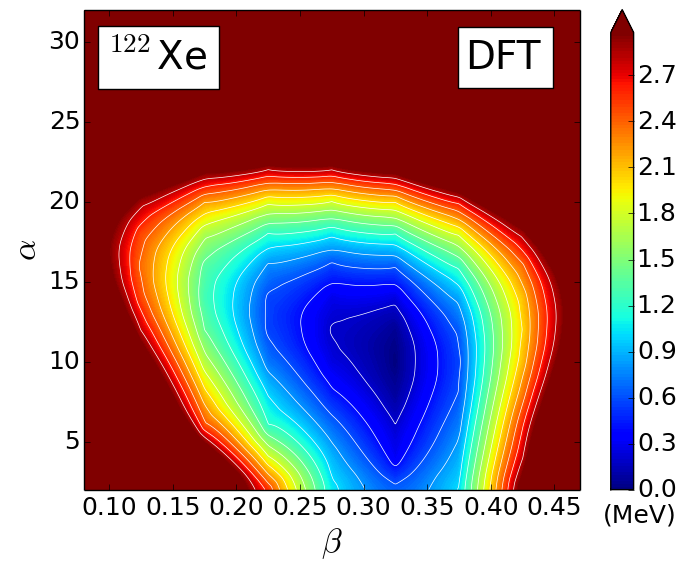
Figure 1: (Color online) The potential energy surface (PES) of ¹²²Xe in the $(\beta,\alpha)$ plane, calculated by the constrained RMF+BCS with the PC-PK1 energy density functional and separable pairing interaction. All energies (in MeV) in the PES are normalized with respect to the binding energy of the absolute minimum. The contours join points on the surface with the same energies, and energy difference between the neighbouring contours is 200 keV.

III Pairing vibrations in the IBM

III.1 The Hamiltonian

In the next step we introduce a model that relates the SCMF ($\beta,\alpha$) potential energy surface (PES) to an equivalent system of interacting bosons. The boson space comprises monopole $s$ and quadrupole $d$ bosons, which represent correlated $L=0^{+}$ and $2^{+}$ pairs of valence nucleons Otsuka et al. (1978b, a); Iachello and Arima (1987). In the conventional IBM, the number of bosons, denoted as $n$, is conserved for a given nucleus, i.e., $n=n_{s}+n_{d}$, where $n_{s}$ and $n_{d}$ stand for the $s$ and $d$ boson number, respectively. The boson number is equal to half the number of valence nucleons counted from the nearest closed shells and, in the illustrative case ¹²²Xe, the boson core nucleus is ¹³²Sn and hence $n=9$. We do not distinguish between neutron and proton degrees freedom in the boson space. Considering the underlying microscopic structure, the monopole pair transfer operator in the bosonic system should be expressed, to a good approximation, in terms of the $s$ boson degree of freedom, i.e., $\hat{P}\propto s^{\dagger}+s$. Hence the $s$ boson is expected to be the most relevant for a description of the pairing vibration mode.

To take explicitly into account the pairing vibration mode, the boson configuration space is extended in such a way that the total number of bosons is no longer conserved, but is allowed to change in the boson number by one, that is, $8\leqslant n\leqslant 10$ for the illustrative case of ¹²²Xe. The following IBM Hamiltonian is employed:

$$\hat{H}= \sum_{n}\hat{\mathcal{P}}_{n}(\epsilon_{s}^{0}\hat{n}_{s}+\epsilon_{d}^{0}\hat{n}_{d}+\kappa\hat{Q}\cdot\hat{Q}+\kappa^{\prime}\hat{L}\cdot\hat{L})\hat{\mathcal{P}}_{n}$$

$$+\sum_{n\neq n^{\prime}}\hat{\mathcal{P}}_{n}t_{s}(s^{\dagger}+s)\hat{\mathcal{P}}_{n^{\prime}}$$ (5)

where $\hat{\mathcal{P}}_{n}$ is the projection operator onto the subspace $[n]$. The parameters for the Hamiltonian could differ between different configuration spaces, but here the same parameters are used for the three configurations. Therefore, for brevity, in the following the operator $\hat{\mathcal{P}}_{n}$ will be omitted, unless otherwise specified. The first and second terms in Eq. (III.1) are the $s$ and $d$ boson-number operators with $\hat{n}_{s}=s^{\dagger}\cdot s$ and $\hat{n}_{d}=d^{\dagger}\cdot\tilde{d}$. $\epsilon_{s}^{0}$ and $\epsilon_{d}^{0}$ are absolute values of the single $s$ and $d$ boson energies. The third term is the quadrupole-quadrupole interaction with the boson quadrupole operator $\hat{Q}=s^{\dagger}\tilde{d}+d^{\dagger}s+\chi(d^{\dagger}\times\tilde{d})^{(2)}$. The fourth term, with the boson angular momentum operator $\hat{L}=\sqrt{10}(d^{\dagger}\times\tilde{d})^{(1)}$, makes a significant contribution to the moments of inertia of the $K^{\pi}=0^{+}$ bands. The last term with strength $t_{s}$ in the above Hamiltonian represents the one $s$-boson (monopole pair) transfer operator. It is the boson-number non-conserving term, and thus mixes the subspaces $[n-1]$, $[n]$, and $[n+1]$. For later convenience, and since the total boson number operator is given as $\hat{n}=\hat{n}_{s}+\hat{n}_{d}$, the above Hamiltonian is rewritten in the form:

$$\hat{H}=\epsilon_{s}^{0}\hat{n}+\epsilon_{d}\hat{n}_{d}+\kappa\hat{Q}\cdot\hat{Q}+\kappa^{\prime}\hat{L}\cdot\hat{L}+t_{s}(s^{\dagger}+s)$$ (6)

where $\epsilon_{d}$ is the $d$-boson energy relative to the $s$ boson one, i.e., $\epsilon_{d}=\epsilon^{0}_{d}-\epsilon^{0}_{s}$. The first term $\epsilon_{s}^{0}\hat{n}$ does not contribute to the relative excitation spectra, and is thus neglected in most IBM calculations. In the present framework, however, since we allow for the boson number to vary, this global term is expected to play an important role, especially for excitation energies of the $0^{+}$ states.

The Hamiltonian Eq. (6) is diagonalized in the following $M$-scheme basis with $M=0$, expressed as a direct sum of the bases for the three configurations:

$$\ket{\Phi}=[\ket{(sd)^{n-1}}\oplus\ket{(sd)^{n}}\oplus\ket{(sd)^{n+1}}]_{M=0},$$ (7)

where $M$ denotes the $z$-projection of the total angular momentum $I$. The value of $I$ for a given eigenstate is identified by calculating the expectation value of the angular momentum operator squared, which should give the eigenvalue $I(I+1)$.

The present computational scheme is formally similar to IBM configuration-mixing calculations that describe the phenomenon of shape coexistence Nomura et al. (2016b). In the conventional configuration-mixing IBM framework, several different boson Hamiltonians are allowed to mix Duval and Barrett (1981). Each of these independent (unperturbed) Hamiltonians is associated with a $2m$-particle-$2m$-hole ($m\in\mathbb{Z}$) excitation from a given major shell to the next and, since in the IBM there is no distinction between particles and holes, differ in boson number by two. The configuration-mixing IBM thus does not conserve the boson number, similar to the present case. Here, however, the model space comprises a single major shell, and the boson number conservation is violated not by the contribution from next major shell (i.e., pair transfer across the shell closure), but by pairing vibrations.

III.2 The boson condensate

The IBM analogue of the $(\beta,\alpha)$ PES is formulated analytically by taking the expectation value of the Hamiltonian of Eq. (III.1) in the boson coherent state $\ket{\Psi(\vec{\alpha})}$ Ginocchio and Kirson (1980); Bohr and Mottelson (1980); Hatch and Levit (1982):

$$\ket{\Psi({\vec{\alpha}})}=\ket{\Psi(n-1,{\vec{\alpha}})}\oplus\ket{\Psi(n,{\vec{\alpha}})}\oplus\ket{\Psi(n+1,{\vec{\alpha}})},$$ (8)

where $\vec{\alpha}$ represents variational parameters. Since here the IBM model space comprises three different boson-number configurations, the above trial wave function is expressed as a direct sum of three independent coherent states. Each of them is given by

$$\ket{\Psi(n,{\vec{\alpha}})}=\frac{1}{\sqrt{n!}}(b_{c}^{\dagger})^{n}\ket{0},$$ (9)

and the condensate boson $b_{c}$ is defined as

$$b_{c}=(\alpha_{0}^{2}+\alpha_{2}^{2})^{-1/2}(\alpha_{0}s+\alpha_{2}d_{0}),$$ (10)

where the amplitudes $\alpha_{0}$ and $\alpha_{2}$ should be related to the pairing deformation $\alpha$ and the axial deformation parameter $\beta$ in the SCMF calculation, respectively. The variable $\alpha_{2}$ can be considered as the shape deformation parameter in the collective model:

$$\alpha_{2}=\bar{\beta},$$ (11)

where $\bar{\beta}$ is the IBM analog of the axially symmetric SCMF deformation parameter. We propose to perform the following coordinate transformation for the variable $\alpha_{0}$:

$$\alpha_{0}=\cosh{(\bar{\alpha}-\bar{\alpha}_{\mathrm{min}})}.$$ (12)

The new coordinate $\bar{\alpha}$ is equivalent to the pairing deformation $\alpha$. $\bar{\alpha}_{\mathrm{min}}$ stands for the $\bar{\alpha}$ value corresponding to the global minimum on the IBM PES. We assume the following relations that relate the amplitudes $\bar{\beta}$ and $\bar{\alpha}$ in the boson system to the $\beta$ and $\alpha$ coordinates of the SCMF model:

$$\bar{\beta}=C_{\beta}\beta,\quad\bar{\alpha}=C_{\alpha}\alpha.$$ (13)

The dimensionless coefficients of proportionality $C_{\beta}$ and $C_{\alpha}$ are additional scale parameters determined by the mapping.

Since our model space comprises three subspaces with different number of bosons, the PES of the boson system is expressed in a matrix form Frank et al. (2004):

$$\Biggr{(}\begin{array}[]{ccc}E_{n-1,n-1}(\bar{\alpha},\bar{\beta})&E_{n-1,n}(\bar{\alpha},\bar{\beta})&0\\ E_{n,n-1}(\bar{\alpha},\bar{\beta})&E_{n,n}(\bar{\alpha},\bar{\beta})&E_{n,n+1}(\bar{\alpha},\bar{\beta})\\ 0&E_{n+1,n}(\bar{\alpha},\bar{\beta})&E_{n+1,n+1}(\bar{\alpha},\bar{\beta})\end{array}\Biggl{)}$$ (17)

In the limit in which boson number is conserved, only the diagonal element $E_{n,n}$ is considered. The energy-surface matrix of Eq. (17) is diagonalized at each point on the surface ($\bar{\beta},\bar{\alpha}$), resulting in three energy surfaces Frank et al. (2004). The usual procedure in most IBM calculations with configuration mixing is to retain only the lowest energy eigenvalue at each deformation.

The analytical expressions for the diagonal and non-diagonal elements of the matrix Eq. (17) are obtained by calculating expectation values of the Hamiltonian Eq. (6) in the coherent state Eq. (10), with the amplitudes defined in Eqs. (11) and (12). The right-hand side of Eq. (12) is Taylor expanded: $\cosh{\bar{\alpha}^{\prime}}=1+\bar{\alpha}^{\prime 2}/2+\mathcal{O}(\bar{\alpha}^{\prime 4})$, and thus $\cosh^{2}{\bar{\alpha}^{\prime}}=1+\bar{\alpha}^{\prime 2}+\mathcal{O}(\bar{\alpha}^{\prime 4})$, where $\bar{\alpha}^{\prime}\equiv\bar{\alpha}-\bar{\alpha}_{\mathrm{min}}$. Terms of the order of $\mathcal{O}(\bar{\alpha}^{\prime 4})$ and higher are hereafter neglected. The resulting analytical expressions for the matrix elements in Eq. (17) read:

$$E_{n,n}(\bar{\alpha},\bar{\beta})=\epsilon^{0}_{s}n+\frac{n[5\kappa+(\epsilon_{d}+6\kappa^{\prime}+\kappa(1+\chi^{2}))\bar{\beta}^{2}]}{1+\bar{\alpha}^{\prime 2}+\bar{\beta}^{2}}$$

$$+\frac{\kappa n(n-1)}{(1+\bar{\alpha}^{\prime 2}+\bar{\beta}^{2})^{2}}\Biggl{[}4(1+\bar{\alpha}^{\prime 2})\bar{\beta}^{2}-4\sqrt{\frac{2}{7}}\chi\bar{\beta}^{3}+\frac{2}{7}\chi^{2}\bar{\beta}^{4}\Biggr{]},$$ (18)

for the diagonal elements, and

$$E_{n,n^{\prime}}(\bar{\alpha},\bar{\beta})=E_{n^{\prime},n}(\bar{\alpha},\bar{\beta})=t_{s}\frac{2\sqrt{n+1}}{\sqrt{1+\bar{\alpha}^{\prime 2}+\bar{\beta}^{2}}},$$ (19)

for the non-diagonal elements with $n>n^{\prime}$. The term proportional to $\bar{\alpha}^{\prime 2}\bar{\beta}^{3}$ in the numerator of the third term of Eq. (III.2), and the term quadratic in $\bar{\alpha}^{\prime}$ in the numerator of Eq. (19) are neglected.

The functional forms in Eqs. (III.2) and (19), in particular the norm factor $\mathcal{N}=1+\bar{\alpha}^{\prime 2}+\bar{\beta}^{2}$ that depends quadratically on $\bar{\alpha}$, most effectively produce an $\alpha$-deformed equilibrium state that is consistent with the SCMF PES. The form of the norm factor ${\mathcal{N}}$ ensures that no divergence occurs at $\bar{\beta}\approx 0$ and $\bar{\alpha}^{\prime}\approx 0$. In the limit $\bar{\alpha}\to\bar{\alpha}_{\rm min}(=C_{\alpha}\alpha_{\mathrm{min}})$, the expression for $E_{n,n}(\bar{\alpha},\bar{\beta})$ reduces to the one used in standard $sd$-IBM calculations Ginocchio and Kirson (1980); Iachello and Arima (1987).

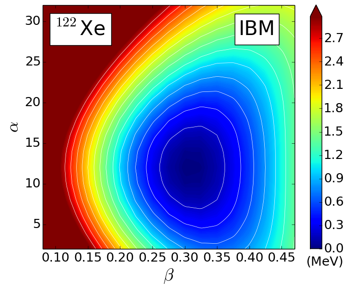
Figure 2: (Color online) Same as in the caption to Fig. 1 but for the IBM energy surface.

III.3 Mapping the boson Hamiltonian

The ${\mathit{p}v}$-IBM Hamiltonian in Eq. (6) is constructed in the following steps:

1. The strength parameters that appear in the boson number conserving part of the Hamiltonian: $\epsilon_{d}$, $\kappa$, and $\chi$, as well as the scale factor $C_{\beta}$, are determined so that the diagonal matrix element $E_{n,n}(\bar{\alpha},\bar{\beta})$ reproduces the SCMF PES at $\alpha=\alpha_{\rm min}$.

2. The strength $\kappa^{\prime}$ of the rotational $\hat{L}\cdot\hat{L}$ term is determined separately so that the bosonic moment of inertia calculated in the intrinsic frame Schaaser and Brink (1986) at the global minimum, should equal the Inglis-Belyaev Inglis (1956); Beliaev (1961) moment of inertia at the corresponding configuration on the SCMF energy surface. The details of this procedure can be found in Ref. Nomura et al. (2011).

3. The $s$ boson energy $\epsilon^{0}_{s}$ and mixing strength $t_{s}$, as well as the scale factor $C_{\alpha}$, are determined in the $(\bar{\beta},\bar{\alpha})$ plane so that the lowest eigenvalue of the energy surface matrix Eq. (17) reproduces the topology of the SCMF PES in the neighbourhood of the equilibrium minimum.

Table 1: Strength parameters of the boson Hamiltonian Eq. (6) determined by mapping the SCMF $(\beta,\alpha)$ energy surface to the boson space. The parameters $\chi$, $C_{\beta}$, and $C_{\alpha}$ are dimensionless, while the others are in units of MeV.

$\epsilon_{s}^{0}$	$\epsilon_{d}$	$\kappa$	$\chi$	$\kappa^{\prime}$	$t_{s}$	$C_{\beta}$	$C_{\alpha}$
2.19	0.611	$-0.102$	$-0.4$	$-0.029$	0.18	2.75	0.045

The values of the resulting parameters of the IBM Hamiltonian are listed in Table 1, and the corresponding IBM PES is shown in Fig. 2. Consistent with the SCMF PES, the equilibrium minimum of the IBM PES is found at $\beta\approx 0.32$ and $\alpha\approx 10$. The potential energy surfaces exhibit a similar topography except for the fact that, away from the global minimum, the IBM surface tends to be softer than the DFT one obtained using the constrained SCMF method. This is a common characteristic of the IBM Nomura et al. (2008) that arises because of the more restricted boson model space as compared to the SCMF approach based on the Kohn-Sham DFT. The former is built only from the valence nucleons, while the latter model space contains all nucleons. Therefore, the boson Hamiltonian parameters are determined by the mapping procedure that is carried out in the neighbourhood of the global minimum, as this region is most relevant for low-energy excitations. The Hamiltonian Eq. (6) is diagonalised in the $M$-scheme basis of Eq. (7).

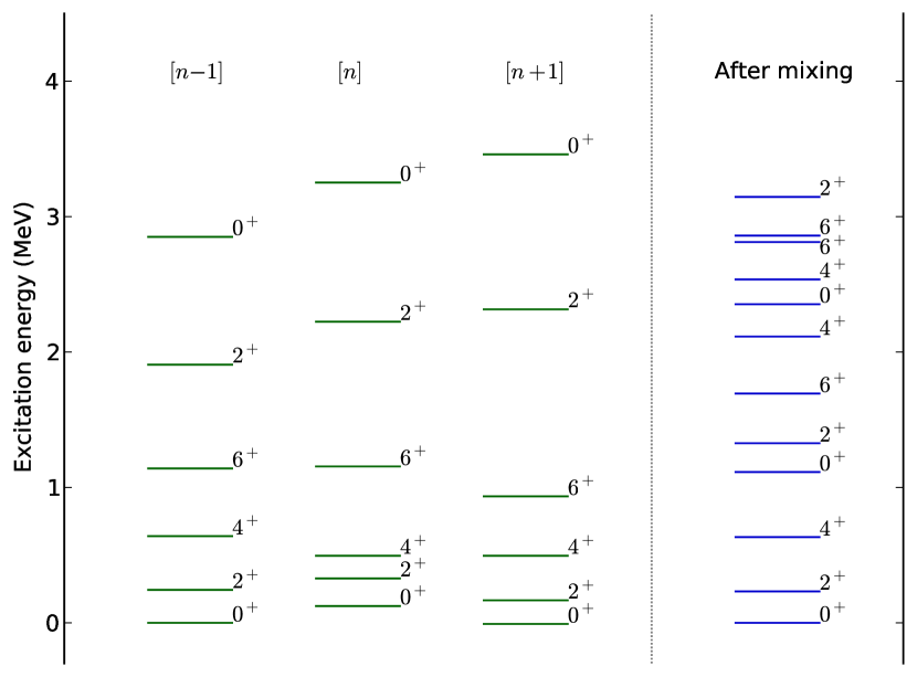
Figure 3: (Color online) Excitation spectra for the unperturbed boson configurations $[n-1]$, $[n]$ and $[n+1]$, and the final one obtained after mixing the three configurations.

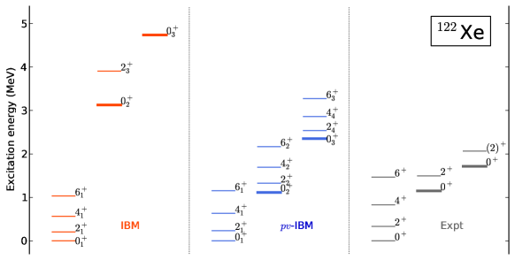
Figure 4: (Color online) Excitation spectra of ¹²²Xe resulting from the IBM calculation with a single boson-number configuration $[n=9]$ (left panel), and including configuration mixing between $[n=8]$, $[n=9]$, and $[n=10]$ boson spaces (${\mathit{p}v}$-IBM). Experimental states are from Refs. Brookhaven National Nuclear Data Center ; Garrett et al. (2017) (right panel). The $0^{+}$ band-head states of the $K^{\pi}=0^{+}$ bands are highlighted with thick lines.

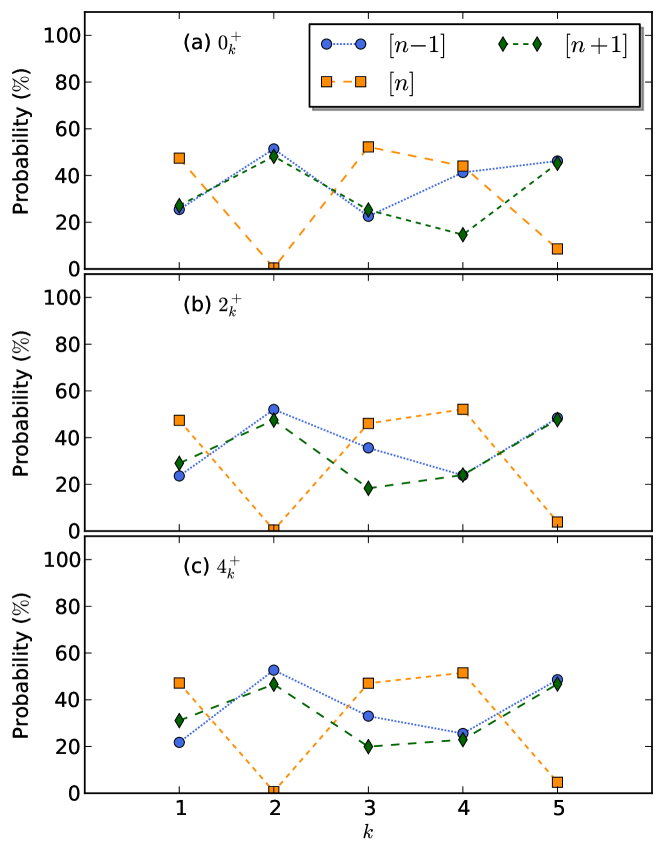
Figure 5: (Color online) Probabilities of the $[n-1]$, $[n]$, and $[n+1]$ components in the wave functions of the five lowest-energy $0^{+}$, $2^{+}$, and $4^{+}$ states in ¹²²Xe.

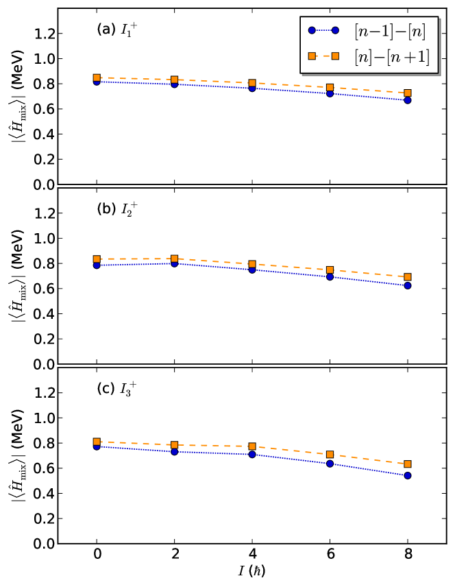
Figure 6: (Color online) Matrix elements of the monopole pair transfer operator $\hat{H}_{\mathrm{mix}}$ (last term in Eq. (6)) between the unperturbed $[n-1]$ and $[n]$ configurations, and between the unperturbed $[n]$ and $[n+1]$ configurations, for the lowest three even-spin states up to $I=8^{+}$.

IV Illustrative example: ¹²²Xe

IV.1 Energy spectra

Figure 3 depicts the calculated excitation spectra corresponding to the unperturbed boson configurations $[n-1]$, $[n]$ and $[n+1]$, and the spectrum obtained by mixing the three different configurations. Without mixing, the $0^{+}$ ground states for the three configurations cluster together within a small energy range, and the first excited $0^{+}$ states are also found in a narrow interval around 3 MeV. This is, of course, easy to understand because the spaces in which the Hamiltonian is diagonalized only differ by $\Delta n=1$ in the boson number. Allowing for configuration mixing (boson-number non-conserving term in the Hamiltonian Eq. (6)), states with the same spin repel and the two lowest $0^{+}$ excited states are found at excitation energies $E_{\mathrm{exc}}\approx 1$ MeV and above $2$ MeV. This shows that, using only a single configuration and fixed boson number, the model cannot reproduce the excitation energies of low-lying $0^{+}$ states. Mixing configurations that correspond to different boson numbers will be essential for the description of low-energy $0^{+}$ excitations.

Figure 4 compares the excitation spectra for ¹²²Xe calculated using the IBM with a single configuration $[n]$, where the boson number $n=9$ is conserved and the effect of the pairing vibration is not taken into account (left-hand panel, (a)), with those obtained with the IBM that includes pairing-vibrations (${\mathit{p}v}$-IBM), shown in the central panel (b)). Part of the available experimental energy spectra Brookhaven National Nuclear Data Center ; Garrett et al. (2017) is also shown in the right-hand panel of Fig. 4. The theoretical states are grouped into bands according to the sequence of calculated E2 strength values. Since we aim to describe excited $0^{+}$ states, only bands that are built on a $0^{+}$ state and that follow the $\Delta I=2$ E2 transition systematics are shown in the figure. The remarkable result is that the $K^{\pi}=0^{+}$ bands built on the $0^{+}_{2}$ and $0^{+}_{3}$ states are dramatically lowered in energy by taking into account configuration mixing, that is, by the inclusion of pairing vibrations. The resulting excitation spectrum is in much better agreement with experiment.

IV.2 Structure of wave functions

To shed more light upon the nature of excited states calculated in the ${\mathit{p}v}$-IBM, we show in Fig. 5 the probabilities of the three different boson-space configurations $[n-1]$, $[n]$, and $[n+1]$ in the lowest five $0^{+}$, $2^{+}$, and $4^{+}$ states of ¹²²Xe. Let us consider, for example, the $0^{+}$ states. Only half the wave function of the ground state $0^{+}_{1}$ is accounted for by the $[n]$ configuration, while the rest is equally shared by the $[n-1]$ and $[n+1]$ configurations. The $0^{+}_{2}$ state exhibits a structure that is completely different from the ground state. The dominant contributions come from the $[n-1]$ and $[n+1]$ configurations, both with probabilities of nearly 50 %, whereas there is almost no contribution from the $[n]$ configuration space. The structure of the $0^{+}_{3}$ state is very similar to that of the $0^{+}_{1}$. The state $0^{+}_{4}$ appears to be different from the lower ones in that the three configurations are more equally mixed: the $[n]$ and $[n-1]$ components are found with approximately 40 % probability each, and the remaining 20 % belongs to the $[n+1]$ configuration space. The content of the $0^{+}_{5}$ wave function is similar to that of $0^{+}_{2}$. A corresponding structure is also found for the $2^{+}$ and $4^{+}$ states. The only exception is perhaps the fourth lowest state of $2^{+}$ and $4^{+}$, nevertheless in each state $0^{+}_{4}$, $2^{+}_{4}$, and $4^{+}_{4}$ the largest contribution to their wave function comes from the $[n]$ configuration.

IV.3 Mixing matrix elements

Figure 6 displays the matrix elements of the mixing interaction $|\braket{I^{+}_{k}}{\hat{H}_{\mathrm{mix}}}{I^{+}_{k}}|$ ($I$ even, $k=1,2,3$), with $\hat{H}_{\mathrm{mix}}=t_{s}(s^{\dagger}+s)$, that couple the unperturbed $[n-1]$ and $[n]$ configurations, and the unperturbed $[n]$ and $[n+1]$ configurations. For all of the unperturbed $I_{1,2,3}$ states, the mixing between the $[n-1]$ and $[n]$ configurations is almost identical to the coupling between the $[n]$ and $[n+1]$ configurations. In both cases the mixing is generally stronger between states with lower spin, and gradually decreases in magnitude as the angular momentum increases.

IV.4 Electromagnetic transitions

The electric quadrupole (E2) and monopole (E0) transition rates can also be analyzed in the ${\mathit{p}v}$-IBM. The corresponding operators are defined as

$$\hat{T}^{E2}=e_{\mathrm{B}}\hat{Q}$$ (20)

$$\hat{T}^{E0}=\xi\hat{n}_{d}+\eta\hat{n}$$ (21)

with $e_{\mathrm{B}}$ is the E2 boson effective charge, and $\xi$ and $\eta$ are parameters. The $B(E2)$ and $\rho^{2}(E0)$ transition rates are then calculated using the relations:

$$B(E2;I_{i}\to I^{\prime}_{j})=\frac{1}{2I_{i}+1}|\braket{I^{\prime}_{j}}{\hat{T}^{E2}}{I_{i}}|^{2}$$ (22)

$$\rho^{2}(E0;I_{i}\to I_{j})=\frac{Z^{2}}{e^{2}r_{0}^{4}A^{4/3}}\frac{1}{2I_{i}+1}|\braket{I_{j}}{\hat{T}^{E0}}{I_{i}}|^{2}\;.$$ (23)

Table 2: $B({E2};I_{i}\to I^{\prime}_{j})$ values in Weisskopf units, calculated in the IBM and ${\mathit{p}v}$-IBM. The experimental values are taken from ENSDF database.

	IBM	${\mathit{p}v}$-IBM	Experiment
$B({{E2}};2^{+}_{1}\to 0^{+}_{1})$	80	79	78(4)
$B({{E2}};4^{+}_{1}\to 2^{+}_{1})$	113	114	114(6)
$B({{E2}};6^{+}_{1}\to 4^{+}_{1})$	121	124	1.1$\times 10^{2}$(4)
$B({{E2}};2^{+}_{K=0^{+}_{2}}\to 0^{+}_{K=0^{+}_{2}})$	46	79
$B({{E2}};4^{+}_{K=0^{+}_{2}}\to 2^{+}_{K=0^{+}_{2}})$	57	111
$B({{E2}};6^{+}_{K=0^{+}_{2}}\to 4^{+}_{K=0^{+}_{2}})$	64	119

Table 3: Reduced matrix elements of the $d$-boson number operator $\hat{n}_{d}$ and the total boson number operator $\hat{n}$ for E0 transitions between the lowest three IBM and ${\mathit{p}v}$-IBM states $0^{+}$ and $2^{+}$ of ¹²²Xe.

		IBM	${\mathit{p}v}$-IBM
$I^{+}_{i}$	$I^{+}_{j}$	$\braket{I_{j}}{\hat{n}_{d}}{I_{i}}$	$\braket{I_{j}}{\hat{n}_{d}}{I_{i}}$	$\braket{I_{j}}{\hat{n}}{I_{i}}$
$0^{+}_{2}$	$0^{+}_{1}$	$-1.166$	0.473	0.721
$0^{+}_{3}$	$0^{+}_{1}$	$-1.139$	0.006	0.017
$0^{+}_{3}$	$0^{+}_{2}$	$-0.431$	0.451	0.687
$2^{+}_{2}$	$2^{+}_{1}$	$-0.503$	$-0.947$	$-1.609$
$2^{+}_{3}$	$2^{+}_{1}$	2.714	$-0.482$	0.084
$2^{+}_{3}$	$2^{+}_{2}$	0.752	$-0.173$	$-0.017$

In Table 2 we compare the $B(E2)$ values calculated with (${\mathit{p}v}$-IBM) and without (IBM) the inclusion of dynamical pairing. A typical value for the E2 effective charge $e_{\mathrm{B}}=0.11$ $e\cdot$b is used both in the IBM and ${\mathit{p}v}$-IBM calculations. The $B(E2)$ transitions between the yrast states do not change by the inclusion of the pairing degree of freedom. The results of both calculations are consistent with the experimental values Brookhaven National Nuclear Data Center . In the ${\mathit{p}v}$-IBM calculation, the E2 transitions in the $0^{+}_{2}$-based band display a more pronounced collectivity, comparable to that in the ground state band. As shown in Fig. 5, in the ${\mathit{p}v}$-IBM wave functions we find a rather large contribution from the $[n+1]$ configurations to the $0^{+}_{2}$ band, and this accounts for the enhanced $B(E2)$ strengths within this sequence of states.

Since there are no data for the $E0$ transitions in ¹²²Xe, in Table 3 we compare the calculated reduced matrix elements of the $\hat{n}_{d}$ and $\hat{n}$ operators, which constitute the E0 operator of Eq. (21). Note that in the number-conserving IBM only the $\hat{n}_{d}$ term contributes. From Table 3 one notices that the reduced matrix elements $\braket{I_{j}}{\hat{n}_{d}}{I_{i}}$ in the ${\mathit{p}v}$-IBM calculation are systematically smaller in magnitude than the corresponding quantity in the IBM, most notably for the $0^{+}_{3}\to 0^{+}_{1}$ transition. The matrix element $\braket{I_{j}}{\hat{n}}{I_{i}}$ is generally of equal magnitude as that of $\hat{n}_{d}$ and, therefore, one expects that it will give a sizeable contribution to the $\rho^{2}(E0)$ values in ${\mathit{p}v}$-IBM.

V Application to $N=92$ isotones

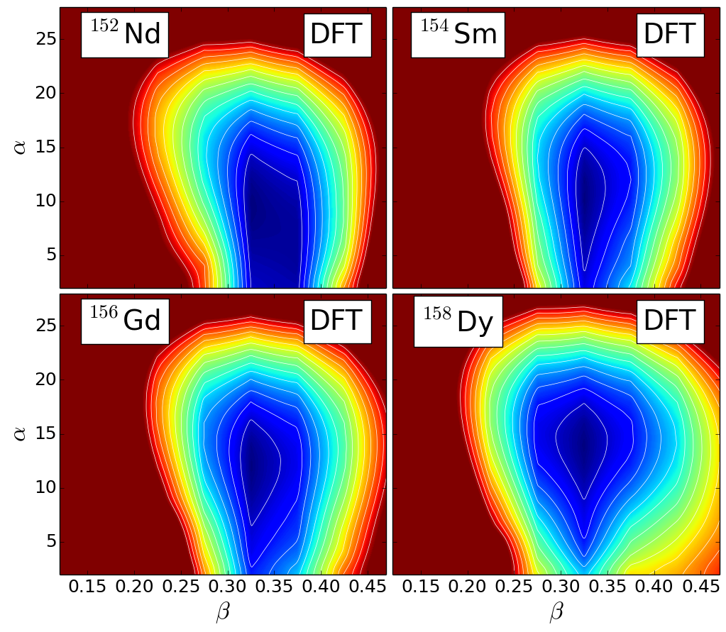
Figure 7: (Color online) Same as in the caption to Fig. 1 but for the $N=92$ isotones ¹⁵²Nd, ¹⁵⁴Sm, ¹⁵⁶Gd, and ¹⁵⁸Dy.

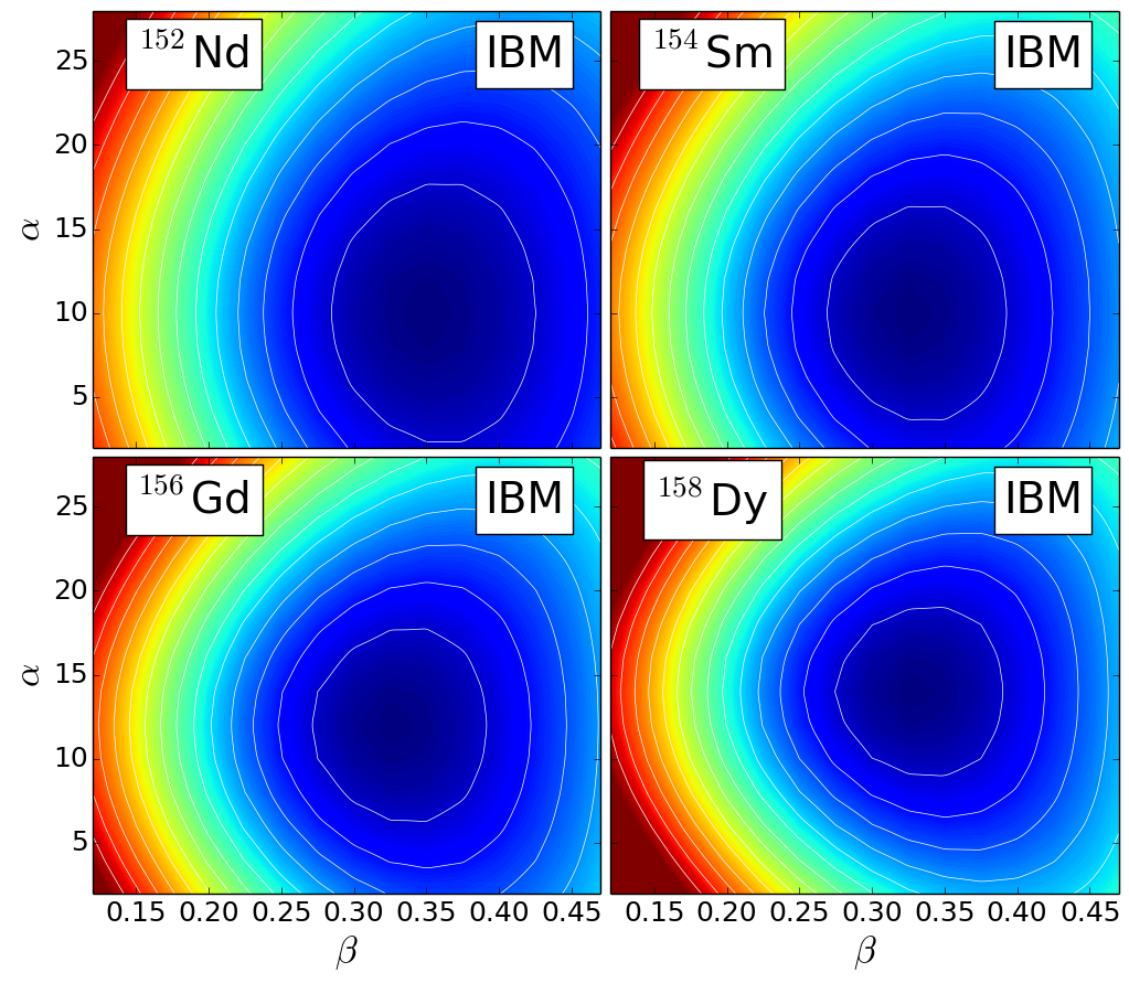
Figure 8: (Color online) Same as in the caption to Fig. 7, but for the IBM energy surfaces.

For a more detailed analysis, we apply the ${\mathit{p}v}$-IBM theoretical framework to a study of the structure of the axially-symmetric $N=92$ rare-earth isotones. For nuclei in this region of the nuclear chart, an unexpectedly large number of low-energy excited $0^{+}$ states have been observed Aprahamian et al. (2018); Majola et al. (2019). From a theoretical point of view, they have been interpreted in terms of pairing vibrations Xiang et al. (2020), contributions of intruder orbitals Van Isacker et al. (1982), and excitations of double octupole phonons Zamfir et al. (2002); Nomura et al. (2015). The occurrence of low-lying excited $0^{+}$ states also characterizes the quantum shape-phase transition from spherical to axially-deformed nuclear systems Cejnar et al. (2010).

V.1 $(\beta,\alpha)$ potential energy surfaces

In Fig. 7 we plot the SCMF deformation energy surfaces in the $(\beta,\alpha)$ plane for the $N=92$ isotones: ¹⁵²Nd, ¹⁵⁴Sm, ¹⁵⁶Gd, and ¹⁵⁸Dy. Note that this is the same as Fig. 7 in Ref. Xiang et al. (2020), in which the coupling of shape and pairing vibrations was analyzed using a collective Hamiltonian based on nuclear DFT. Pronounced axially symmetric global minima are calculated at $\beta\approx 0.35$. The deformation surfaces are much softer with respect to the pairing deformation $\alpha$, and the minima extend in a rather large interval $5\leqslant\alpha\leqslant 15$. As already noted in Ref. Xiang et al. (2020), this softness is reduced with the increase of the proton number, while simultaneously the energy surfaces become more soft in the quadrupole collective deformation.

Table 4: Same as the caption Table 1, but for the $N=92$ isotones.

	$\epsilon_{s}^{0}$	$\epsilon_{d}$	$\kappa$	$\chi$	$\kappa^{\prime}$	$t_{s}$	$C_{\beta}$	$C_{\alpha}$
152Nd	1.40	0.478	$-0.045$	$-1.1$	$-0.0130$	0.16	2.85	0.035
154Sm	1.37	0.626	$-0.043$	$-1.1$	$-0.0126$	0.16	2.90	0.040
156Gd	1.30	0.530	$-0.040$	$-0.9$	$-0.0083$	0.14	2.80	0.045
158Dy	1.32	0.533	$-0.038$	$-0.85$	$-0.0054$	0.12	2.75	0.050

The corresponding bosonic energy surfaces in the $(\beta,\alpha)$ plane are drawn in Fig. 8. They exhibit a non-zero $\alpha$ global minimum, consistent with the microscopic SCMF PESs. As already noted above in the case of ¹²²Xe, the IBM PESs are considerably softer than the SCMF ones, especially far from the global minimum. This is due to the more restricted boson model space, that is, the restricted space of valence nucleons from which the bosons are built does not contain the high-energy configurations that contribute to the SCMF solutions far from the equilibrium minimum. The strength parameters of the boson Hamiltonian in Eq. (III.1), determined by mapping the SCMF energy surfaces to the expectation values of the Hamiltonian in the boson condensate, are listed in Table 4 for the $N=92$ isotones . The large negative values of the derived parameter $\chi$ parameter, close to the SU(3) limit of the IBM $\chi_{\mathrm{SU(3)}}=-\sqrt{7}/2$, reflect the pronounced axially-symmetric prolate quadrupole deformation of these nuclei.

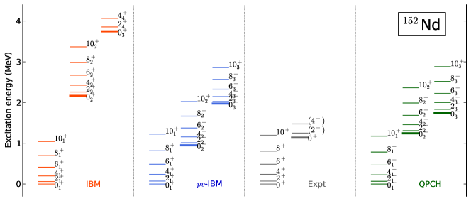
Figure 9: (Color online) Low-energy $K^{\pi}=0^{+}$ bands of ¹⁵²Nd, calculated using the IBM without and with the dynamical pairing degree of freedom, in comparison to available data Brookhaven National Nuclear Data Center . The corresponding spectrum obtained with the Quadrupole-Pairing Collective Hamiltonian (QPCH) model is included for comparison.

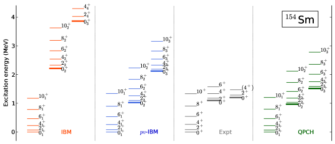
Figure 10: (Color online) Same as in the caption to Fig. 9, but for ¹⁵⁴Sm.

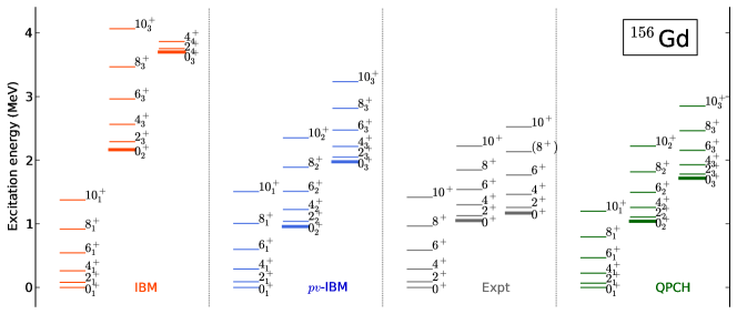
Figure 11: (Color online) Same as in the caption to Fig. 9, but for ¹⁵⁶Gd.

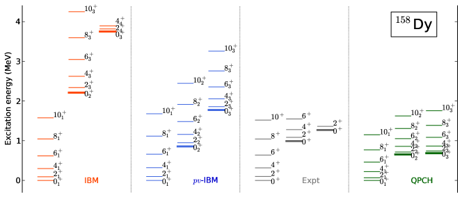
Figure 12: (Color online) Same as in the caption to Fig. 9, but for ¹⁵⁸Dy.

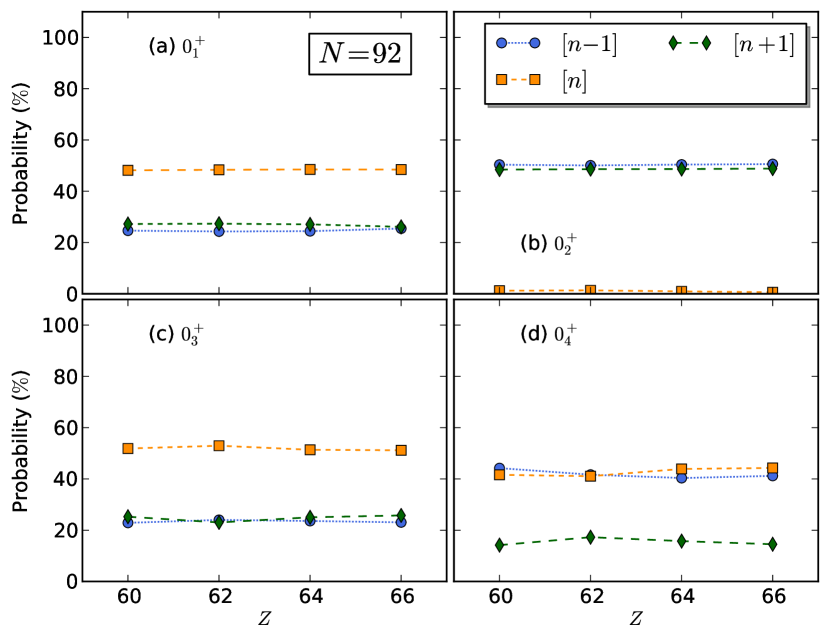
Figure 13: (Color online) Probabilities of the $[n-1]$, $[n]$, and $[n+1]$ components in the ${\mathit{p}v}$-IBM wave functions of the four lowest $0^{+}$ states in the $N=92$ isotones.

V.2 Low-energy excitation spectra

Figures 9, 10, 11, and 12 compare the three-lowest $K^{\pi}=0^{+}$ bands of four $N=92$ isotones: ¹⁵²Nd, ¹⁵⁴Sm, ¹⁵⁶Gd, and ¹⁵⁸Dy, respectively, computed using the IBM and ${\mathit{p}v}$-IBM and IBM. In addition to the corresponding data, we also include the results of our recent study that has used the newly developed Quadrupole-Pairing Collective Hamiltonian (QPCH) to analyze the low-energy spectra of these nuclei Xiang et al. (2020). A detailed description of the QPCH model can be found Ref. Xiang et al. (2020). All three Hamiltonians (IBM, ${\mathit{p}v}$-IBM, and QPCH) used here are based on the same energy density functional and pairing interaction. The excitation spectra shown in Figs. 9-12 clearly illustrate the striking effect of the coupling between shape and pairing degrees of freedom. The inclusion of dynamical pairing significantly lowers the bands based on excited $0^{+}$ states. The bands calculated with ${\mathit{p}v}$-IBM and QPCH are in much better agreement with experiment, especially the band based on $0^{+}_{2}$. We note that the overall quality of the ${\mathit{p}v}$-IBM description of $K^{\pi}=0^{+}$ bands is comparable to that of the fully microscopic QPCH model.

Even though we only show the $K^{\pi}=0^{+}$ bands in Figs. 9-12, the $K^{\pi}=2^{+}$ (or $\gamma$-) bands are also observed experimentally for the $N=92$ isotones. The IBM models can be used to compute these states but, since this study is restricted to axial symmetry, the focus is on $K^{\pi}=0^{+}$ bands. For completeness, the $K=2^{+}_{1}$ bandhead is calculated to be 2.248 (2.315), 2.330 (2.451), 2.102 (2.114), and 2.085 (2.099) MeV, for ¹⁵²Nd, ¹⁵⁴Sm, ¹⁵⁶Gd, and ¹⁵⁸Dy in the ${\mathit{p}v}$-IBM (IBM) calculations, respectively. Thus, in the axial case, the energies of the $\gamma$ band are hardly affected by the inclusion of the pairing degree of freedom. The corresponding experimental $2^{+}_{\gamma}$ energies for ¹⁵⁴Sm, ¹⁵⁶Gd, and ¹⁵⁸Dy are: 1.440 Smallcombe et al. (2014), 1.154 Aprahamian et al. (2018), 0.946 MeV Majola et al. (2019), respectively, whereas no $\gamma$ band has been identified in ¹⁵²Nd. Therefore we note that, for a quantitative comparison with data, the theoretical framework should be extended with the $\gamma$ degree of freedom (non-axial shapes).

V.3 Structure of the wave functions

In Fig. 13 we plot the probabilities of the three different boson configurations $[n-1]$, $[n]$, and $[n+1]$ in the ${\mathit{p}v}$-IBM wave functions of the four lowest-energy $0^{+}$ states. In all four $N=92$ isotones nearly half of the wave function of the $0^{+}_{1}$ ground state (a) is accounted for by the $[n]$ configuration. The structure of wave function for the $0^{+}_{2}$ state is based mainly on the $[n-1]$ and $[n+1]$ configurations, with almost no contribution from the states of the $[n]$-boson model space. The $0^{+}_{3}$ state is mainly composed of $[n]$-boson configurations, similar to the $0^{+}_{1}$ ground state. The wave function of the $0^{+}_{4}$ state (d) somewhat differs in structure from the lower-energy $0^{+}$ states: each of the $[n]$ and $[n-1]$ configurations takes approximately 40 % of the wave function, and the remaining 20 % consists of the $[n+1]$ configuration.

Table 5: $B({E2};I_{i}\to I^{\prime}_{j})$ values (in Weisskopf units) for ¹⁵²Nd, ¹⁵⁴Sm, ¹⁵⁶Gd, and ¹⁵⁸Dy. Experimental values Brookhaven National Nuclear Data Center ; Möller et al. (2012); Aprahamian et al. (2018) are compared to results of the ${\mathit{p}v}$-IBM, IBM and QPCH model calculations.

		Expt	${\mathit{p}v}$-IBM	IBM	QPCH
152Nd	$2^{+}_{1}\to 0^{+}_{1}$	173$\pm 10$	160	162	162
	$4^{+}_{1}\to 2^{+}_{1}$	226$\pm 11$	225	227	231
	$6^{+}_{1}\to 4^{+}_{1}$	218${}^{+51}_{-35}$	240	241	253
154Sm	$2^{+}_{1}\to 0^{+}_{1}$	176$\pm 1$	184	186	197
	$4^{+}_{1}\to 2^{+}_{1}$	245$\pm 6$	260	262	282
	$6^{+}_{1}\to 4^{+}_{1}$	289$\pm 8$	280	281	310
	$8^{+}_{1}\to 6^{+}_{1}$	319$\pm 17$	283	281	324
	$0^{+}_{K=0^{+}_{2}}\to 2^{+}_{1}$	11.2$\pm 2.1$	6.0	5.0	5.9
	$2^{+}_{K=0^{+}_{2}}\to 0^{+}_{1}$	0.32$\pm 0.04$	0.7	1.7	1.1
	$2^{+}_{K=0^{+}_{2}}\to 2^{+}_{1}$	0.72$\pm 0.09$	1.4	2.0	1.6
	$2^{+}_{K=0^{+}_{2}}\to 4^{+}_{1}$	1.32$\pm 0.15$	3.7	0.6	3.1
	$4^{+}_{K=0^{+}_{2}}\to 2^{+}_{1}$	0.32$\pm 0.11$	0.7	0.9	1.5
	$4^{+}_{K=0^{+}_{2}}\to 4^{+}_{1}$	0.57$\pm 0.18$	1.2	1.3	1.4
	$4^{+}_{K=0^{+}_{2}}\to 6^{+}_{1}$	0.66$\pm 0.21$	3.7	1.9	2.7
	$2^{+}_{\gamma}\to 0^{+}_{1}$	1.9$\pm 0.2$	0.1	0.3
	$2^{+}_{\gamma}\to 2^{+}_{1}$	3.2$\pm 0.3$	2.4	1.8
	$2^{+}_{\gamma}\to 4^{+}_{1}$	0.36$\pm 0.05$	2.4	2.8
156Gd	$2^{+}_{1}\to 0^{+}_{1}$	189$\pm 3$	195	197	205
	$4^{+}_{1}\to 2^{+}_{1}$	264$\pm 4$	276	279	293
	$6^{+}_{1}\to 4^{+}_{1}$	295$\pm 8$	299	300	322
	$8^{+}_{1}\to 6^{+}_{1}$	320$\pm 17$	304	303	335
	$10^{+}_{1}\to 8^{+}_{1}$	314$\pm 14$	299	296	342
	$0^{+}_{K=0^{+}_{2}}\to 2^{+}_{1}$	8${}^{+4}_{-7}$	4.9	4.3	2.5
	$2^{+}_{K=0^{+}_{2}}\to 0^{+}_{1}$	0.63$\pm 0.06$	0.6	0.8	1.8
	$2^{+}_{K=0^{+}_{2}}\to 0^{+}_{K=0^{+}_{2}}$	52$\pm 23$	196	136	236
	$2^{+}_{K=0^{+}_{2}}\to 2^{+}_{1}$	3.3$\pm 0.3$	1.2	0.5	2.5
	$2^{+}_{K=0^{+}_{2}}\to 4^{+}_{1}$	4.1$\pm 0.4$	3.0	2.9	4.2
	$4^{+}_{K=0^{+}_{2}}\to 2^{+}_{K=0^{+}_{2}}$	330${}^{+110}_{-130}$	276	180	337
	$4^{+}_{K=0^{+}_{2}}\to 2^{+}_{1}$	1.3${}^{+0.5}_{-0.7}$	0.7	0.8	2.6
	$4^{+}_{K=0^{+}_{2}}\to 6^{+}_{1}$	2.1${}^{+0.7}_{-1.1}$	3.0	3.3	3.4
	$0^{+}_{K=0^{+}_{3}}\to 2^{+}_{1}$	1.6${}^{+2.3}_{-0.8}$	0.02	0.02	2.6
	$2^{+}_{\gamma}\to 0^{+}_{1}$	4.68$\pm 0.16$	2.4	2.4
	$2^{+}_{\gamma}\to 2^{+}_{1}$	7.24$\pm 0.25$	6.3	5.8
	$2^{+}_{\gamma}\to 4^{+}_{1}$	0.77$\pm 0.04$	0.2	0.2
158Dy	$2^{+}_{1}\to 0^{+}_{1}$	186$\pm 4$	218	220	199
	$4^{+}_{1}\to 2^{+}_{1}$	266$\pm 15$	309	311	284
	$6^{+}_{1}\to 4^{+}_{1}$	3.4$\times 10^{2}(4)$	335	337	312
	$8^{+}_{1}\to 6^{+}_{1}$	3.4$\times 10^{2}(7)$	342	342	326
	$2^{+}_{\gamma}\to 0^{+}_{1}$	5.9$\pm 1.2$	3.1	3.1
	$2^{+}_{\gamma}\to 2^{+}_{1}$	19$\pm 4$	7.2	6.7
	$2^{+}_{\gamma}\to 4^{+}_{1}$	2.1$\pm 0.8$	0.3	0.3
	$2^{+}_{K=0^{+}_{2}}\to 0^{+}_{1}$	2.1$\pm 0.5$	0.6	0.8	1.6
	$2^{+}_{K=0^{+}_{2}}\to 2^{+}_{1}$	3.5$\pm 0.8$	1.1	0.6	1.8
	$2^{+}_{K=0^{+}_{2}}\to 4^{+}_{1}$	12$\pm 3$	2.8	2.9	2.0

Table 6: Same as the caption to Tab. 5 but for the $\rho^{2}({E0};I_{i}\to I_{j})\times 10^{3}$ values. The experimental $\rho^{2}(E0)$ are from Refs. Brookhaven National Nuclear Data Center ; Bäcklin et al. (1982); Wood et al. (1999); Kibédi and Spear (2005); Wimmer et al. (2009); Smallcombe et al. (2014); Majola et al. (2019).

		Expt	${\mathit{p}v}$-IBM	IBM	QPCH
154Sm	$0^{+}_{2}\to 0^{+}_{1}$	96$\pm 42$	43	39	54
	$2^{+}_{2}\to 2^{+}_{1}$	$\leqslant 9.4\pm 1.5$	41	36	53
	$4^{+}_{2}\to 4^{+}_{1}$	8.2${}^{+12.0}_{-8.2}$	38	28	53
156Gd	$0^{+}_{2}\to 0^{+}_{1}$	42$\pm 21$	42	43	73
	$0^{+}_{3}\to 0^{+}_{1}$	1.2${}^{+1.9}_{-0.6}$	0.2	1.8	13
	$0^{+}_{3}\to 0^{+}_{2}$	18${}^{+27}_{-9}$	41	40	97
	$0^{+}_{4}\to 0^{+}_{1}$	2.9${}^{+2.7}_{-1.4}$	54	0.07	3.4
	$0^{+}_{4}\to 0^{+}_{3}$	6.3${}^{+5.7}_{-3.0}$	0.6	5.6	34
	$2^{+}_{K=0^{+}_{2}}\to 2^{+}_{1}$	54$\pm 4$	40	41	72
	$2^{+}_{K=0^{+}_{3}}\to 2^{+}_{1}$	0.2${}^{+0.6}_{-0.2}$	0.05	0.4	13
	$4^{+}_{K=0^{+}_{2}}\to 4^{+}_{1}$	50${}^{+25}_{-16}$	38	34	72
	$4^{+}_{K=0^{+}_{3}}\to 4^{+}_{1}$	$<15$	4$\times 10^{-5}$	0.08	13
158Dy	$2^{+}_{K=0^{+}_{2}}\to 2^{+}_{1}$	27$\pm 12$	40	48	75

V.4 Transition rates

The $B(E2)$ and $\rho^{2}(E0)$ values calculated with the ${\mathit{p}v}$-IBM, IBM and QPCH models are compared to available data in Tabs. 5 and 6, respectively, The effective boson charge in the E2 operator is $e_{\mathrm{B}}=0.14$ $e\cdot$b. The parameters of the E0 operators: $\xi=0.095$ and $\eta=0.11$ fm² for the ${\mathit{p}v}$-IBM, and $\xi=0.075$ fm² for the IBM, are adjusted to obtain the best agreement with the experimental $\rho^{2}(E0)$ values for ¹⁵⁶Gd, and kept unchanged for all four $N=92$ isotones. There are no adjustable parameters for the calculation of transition rates in the QPCH model. Note that there are no E2 transitions related to the $\gamma$ band with $K^{\pi}=2^{+}$ in the QPCH model since, as pointed out above, the present version of QPCH does not include the triaxial degree of freedom.

As shown in Table 5, the $B(E2)$ transition strengths within the ground state bands are reproduced very nicely by all the models. There is no significant difference between the $B(E2)$ values calculated with the IBM and ${\mathit{p}v}$-IBM. Many experimental results are available for the transition rates of ¹⁵⁴Sm and, generally, they are well reproduced by all three models. In ¹⁵⁶Gd the theoretical results reproduce the data, except for an overestimate of the experimental $B(E2;2^{+}_{K=0^{+}_{2}}\to 0^{+}_{K=0^{+}_{2}})$ value of $52\pm 23$ W.u. Very good results are also obtained for ¹⁵⁸Dy.

The calculated $\rho^{2}(E0)$ values are generally in satisfactory agreement with available data (Table 6), except in the case of ¹⁵⁴Sm, in which both the IBM and QPCH approaches considerably overestimate the measured Smallcombe et al. (2014) upper limits of the $\rho^{2}({E0};2^{+}_{2}\to 2^{+}_{1})$ and $\rho^{2}({E0};4^{+}_{2}\to 4^{+}_{1})$ values. It appears that the IBM and ${\mathit{p}v}$-IBM models reproduce the data somewhat better than QPCH, but this comes at the expense of additional adjustable parameters in the $E0$ operator.

VI Conclusion and outlook

We have developed a model that incorporates the coupling between nuclear shape and pairing degrees of freedom in the framework of the IBM, based on nuclear DFT. To account for pairing vibrations, a boson-number non-conserving IBM Hamiltonian is introduced. The boson model space is then extended from the usual one in which the boson number equals half the number of valence nucleons, to include three subspaces that differ in boson number by one. The three subspaces are mixed by a specific monopole pair transfer operator. In a first step of the construction of the IBM Hamiltonian, a set of constrained SCMF calculation is performed for a specific choice of the universal EDF and pairing force, and with the constraints on the expectation values of the axial mass quadrupole operator and monopole pairing operator. These calculations produce a potential energy surface (PES) in the plane of the axial quadrupole $\beta$ and pairing $\alpha$ collective coordinates. The energy surface is then mapped onto the expectation value of the IBM Hamiltonian in the boson condensate state. The mapping determines the strength parameters of the IBM Hamiltonian, and from the corresponding eigenvalue equation excitation energy spectra and transition rates are obtained.

As a first application of the newly developed model, this work has focused on the excitation spectrum of ¹²²Xe. By the inclusion of the dynamical pairing degree of freedom in the IBM and the resulting boson-number configuration mixing, it has been shown that the excitation energies of the $0^{+}_{2}$ and $0^{+}_{3}$ states and the bands built on them, are dramatically lowered by a factor of two or three, thus bringing the theoretical spectrum in quantitative agreement with experiment. The validity of the method has been further examined in a more systematic study of the axially-symmetric $N=92$ rare-earth isotones. The microscopic coupling between shape and pairing degrees of freedom leads to a boson Hamiltonian that, when compared to the standard IBM, significantly lowers the $K^{\pi}=0^{+}$ bands based on excited $0^{+}$ states in ¹⁵²Nd, ¹⁵⁴Sm, ¹⁵⁶Gd, and ¹⁵⁸Dy. The calculated excitation spectra are in an excellent agreement with experiment, and are fully consistent with the results of the corresponding quadrupole-pairing collective Hamiltonian model Xiang et al. (2020). Both models also reproduce the empirical E2 and E0 transition properties with a reasonable accuracy.

The present study has shown a new interesting possibility for extending the DFT-to-IBM mapping method. By incorporating explicitly the dynamical pairing degree of freedom in the IBM, this model can be used to describe pairing vibrational modes and quantitatively reproduce the excitations of low-energy $0^{+}$ states. Here we have only considered the coupling of the pairing degree of freedom with the axial shape deformation. A more challenging case, but also more realistic, will be the coupling between the pairing and triaxial $(\beta,\gamma)$ shape degrees of freedom. This will be particularly important in $\gamma$-soft nuclei and systems that exhibit shape coexistence. In principle, such an extension is also possible in the QPCH approach, however this generates additional terms in the collective Schrödinger equation that represent the couplings of the $\beta-\gamma$ and $\gamma-\alpha$ variables. In contrast, it is rather straightforward to extend the present IBM framework to triaxial nuclei, since there is no need for new building blocks in the boson Hamiltonian. Work in this direction is in progress, and will be reported in a forthcoming article.