Construction of artificial point sources for a linear wave equation in unknown medium

Abstract: We study the wave equation on a bounded domain of ${\mathbb{R}}^{m}$ and on a compact Riemannian manifold $M$ with boundary. We assume that the coefficients of the wave equation are unknown but that we are given the hyperbolic Neumann-to-Dirichlet map $\Lambda$ that corresponds to the physical measurements on the boundary. Using the knowledge of $\Lambda$ we construct a sequence of Neumann boundary values so that at a time $T$ the corresponding waves converge to zero while the time derivative of the waves converge to a delta distribution. Such waves are called an artificial point source. The convergence of the wave takes place in the function spaces naturally related to the energy of the wave. We apply the results for inverse problems and demonstrate the focusing of the waves numerically in the 1-dimensional case.

Keywords: Focusing of waves, Neumann-to-Dirichlet map, Inverse problems.

AMS classification: 35R30, 93B05

1. Introduction

We consider the wave equation in $M$ that is a bounded domain of ${\mathbb{R}}^{m},\,m\geq 1,$ or a compact manifold. Let $u=u^{f}(x,t)$ be the solution of the wave equation

(1) $$\begin{cases}\partial_{t}^{2}u(x,t)+{\mathcal{A}}u(x,t)=0,\quad\hbox{ in }M\times{\mathbb{R}}_{+},\\ u|_{t=0}=0,\quad\partial_{t}u|_{t=0}=0,\\ \partial_{\nu}u|_{\partial M\times{\mathbb{R}}_{+}}=f,\end{cases}$$

where ${\mathcal{A}}$ is a selfadjoint second order elliptic differential operator of the form

$${\mathcal{A}}=-\Delta_{g}+\sum_{j=1}^{m}V_{j}(x)\partial_{x_{j}},$$

where $\Delta_{g}$ is the Laplace operator associated to a Riemannian metric $g$, see (6) for precise definition. Moreover, $f\in L^{2}(\partial M\times{\mathbb{R}}_{+})$ is a Neumann boundary value that physically corresponds to a boundary source, $u=u^{f}$ is the unique solution wave corresponding to the boundary source $f,$ and $\nu$ is the interior pointing normal vector of the boundary $\partial M.$ We assume that we are given the Neumann-to-Dirichlet map, $\Lambda f=u^{f}|_{\partial M\times{\mathbb{R}}_{+}}$. The map $\Lambda$ corresponds to the knowledge of measurements made on the boundary of the domain and it models the response $u^{f}|_{\partial M\times{\mathbb{R}}_{+}}$ of the medium to a source $f$ put on the boundary of $M$.

We show that using $\Lambda$ we can find a sequence of Neumann boundary values $f_{i}$ such that the wave and its time derivative at the large enough time $T$, that is, the pair $(u^{f_{i}}(\,\cdotp,T),u^{f_{i}}_{t}(\,\cdotp,T))$ converge in the energy norm to $(0,\frac{1}{\hbox{\tiny Vol}(V)}\mathds{1}_{V})$, as $i\to\infty$. Here, $V(x)$ is the indicator function a small neighborhood of a point $\widehat{x}\in M$ and $\hbox{Vol}(V)$ is the Riemannian volume of $V$ in $(M,g)$. More precisely, $\widehat{x}=\gamma_{\widehat{z},\nu}({{\widehat{t}}})$ is a point on the normal geodesics emanating from a boundary point $\widehat{z}$. Furthermore, when the neighborhood $V$ converges to the point $\widehat{x}$, the limits $(0,\frac{1}{\hbox{\tiny Vol}(V)}\mathds{1}_{V})$ converges in suitable function space to $(0,\delta_{\widehat{x}})$, where $\delta_{\widehat{x}}$ is the Dirac delta distribution. We call the waves $u^{f_{i}}$ that concentrate their energy in a small neighbourhood $V$ of a point inside the domain the focusing waves. When $V\to\{\widehat{x}\}$, the waves $u^{f_{i}}(x,t)$ converge in the set $M\times(T,\infty)$ converge to $G(x,t;\widehat{x},T)$, where Green’s function $G(x,t;x_{0},t_{0})$ that is the solution of

(2) $$\begin{cases}\left(\partial^{2}_{t}-\mathcal{A}\right)G(x,t;x_{0},t_{0})=\delta_{x_{0}}(x)\delta_{t_{0}}(t)\quad\hbox{on }M\times{\mathbb{R}}\\ G(\cdot,\cdot;x_{0},t_{0})|_{t<t_{0}}=0;\,\,\partial_{\nu}G(\cdot,\cdot;x_{0},t_{0})|_{\partial M\times{\mathbb{R}}}=0.\end{cases}$$

Roughly speaking, the waves $u^{f_{i}}$ in the set $M\times(T,\infty)$ converge to the wave that is produced at a point source located at $(\widehat{x},T)$. Due to this, we say that when $V\to\{x\}$, the limit of the focusing waves produces an artificial point source at time $t=T$.

We emphasize that the boundary sources $f_{i}$ that produce focusing waves can be determined without knowing the coefficients of the operator ${\mathcal{A}}$, that is, when the medium in $M$ is unknown and it is enough only to know the map $\Lambda$ that corresponds to measurements done on the boundary of the domain. Our main resut is the following:

Theorem 1.1.

Let $T>\frac{1}{2}\hbox{diam }(M)$ and $\widehat{x}={\gamma}_{\widehat{z},\nu}({{{{\widehat{t}}}}})\in M$, $\widehat{z}\in{\partial M}$, $0<{{{{\widehat{t}}}}}<T$. Let $\tau_{\partial M}(\widehat{z})$ be the critical distance along the normal geodesic $\gamma_{\widehat{z},\nu}$, defined in (7).

Then $(\partial M,g|_{\partial M})$ and the Neumann-to-Dirichlet map $\Lambda$ determine Neumann boundary values $f_{n}{{(\alpha,\beta}},k)$, $n,k\in{\mathbb{Z}}_{+},$ $\alpha,\beta>0$, such that the following is true:

If ${{{{{{\widehat{t}}}}}}}<\tau_{\partial M}(\widehat{z})$ then

(3) $$\lim_{\alpha\to 0^{+}}\lim_{\beta\to 0^{+}}\lim_{n\to\infty}\begin{pmatrix}u^{f_{n}{{(\alpha,\beta}},k)}(\cdot,T)\\ \partial_{t}u^{f_{n}{{(\alpha,\beta}},k)}(\cdot,T)\end{pmatrix}=\begin{pmatrix}0\\ \frac{1}{\hbox{\tiny Vol}(\Omega_{k})}\mathds{1}_{\Omega_{k}}\end{pmatrix}\quad\hbox{in $H_{0}^{1}(M)\times L^{2}(M)$},$$

where $\Omega_{k}\subset M$ are neighborhoods of $\widehat{x}$ satisfying $\lim_{k\to\infty}\Omega_{k}=\{\widehat{x}\}$. Moreover,

(4) $$\lim_{k\to\infty}\left(\lim_{\alpha\to 0^{+}}\lim_{\beta\to 0^{+}}\lim_{n\to\infty}\begin{pmatrix}u^{f_{n}{{(\alpha,\beta}},k)}(\cdot,T)\\ \partial_{t}u^{f_{n}{{(\alpha,\beta}},k)}(\cdot,T)\end{pmatrix}\right)=\begin{pmatrix}0\\ \delta_{\widehat{x}}\end{pmatrix},$$

where the inner limits with respect to $n,\beta,\alpha$ are in $H_{0}^{1}(M)\times L^{2}(M)$ and the outer limit with respect to $k$ is in the space $H^{-s+1}(M)\times H^{-s}(M)$ with $s>{\dim(M)}/{2}$. In addition, for $t>T$

(5) $$\lim_{k\to\infty}\left(\lim_{\alpha\to 0^{+}}\lim_{\beta\to 0^{+}}\lim_{n\to\infty}u^{f_{n}{{(\alpha,\beta}},k)}(\,\cdot,t)\right)=G(\,\cdot,t;\widehat{x},T)$$

where the inner limits with respect to $n,\beta,\alpha$ are in $H_{0}^{1}(M)$ and the outer limit with respect to $k$ is in the space $H^{-s+1}(M)$.

If ${{{{{{\widehat{t}}}}}}}>\tau_{\partial M}(\widehat{z})$, then limits (3), (4) and (5) are equal to zero.

The boundary sources $f_{n}{{(\alpha,\beta}},k)$ in Theorem 1.1, that produce an artificial point source, are obtained using an iterative sequence of measurements. In this iteration, we first measure for $n=1$ the boundary value, $\Lambda f_{1}$, of the wave that is produced by a certain boundary source $f_{1}$. In each iteration step, we use the boundary source $f_{n}$ and its response $\Lambda f_{n}$ to compute the boundary source $f_{n+1}$ for the next iteration step. The iteration algorithm in this paper was inspired by time reversal methods, see [2, 3, 9, 8, 16, 17, 22, 35, 36, 37]. We note that when the traditional time-reversal algorithms are used in imaging, one typically needs to assume that the medium contains some point-like scatterers.

Generally, when the coefficients of the operator ${\mathcal{A}}$ are unknown, one can not specify the Euclidean coordinates of the point $\widehat{x}$ to which the waves focus, but only the Riemannian boundary normal coordinates $(\widehat{z},\widehat{t})$ (called also the ray coordinates in optics or the migration coordinates in Earth sciences) of $\widehat{x}$ can be specified. However, in the case when $M\subset{\mathbb{R}}^{m}$ and the operator $\mathcal{A}$ is of the form $\mathcal{A}=-c(x)^{2}\Delta$, we show in Corollary 4.3 that the Euclidean coordinates of the point $\widehat{x}$ can be computed using the Neumann-to-Dirichlet map $\Lambda$.

The problem studied in the paper is motivated by recent advances in the applications of optimal control methods to lithotripsy and hyperthermia. In lithotripsy, one breaks down a kidney or bladder stone using a focusing ultrasonic wave. Likewise, in hyperthermia in medical treatments, cancer tissue is destroyed by ultrasound induced heating that produces an excessive heat dose generated by a focusing wave [34]. Often, to apply these methods one needs to use other physical imaging modalities, for example X-rays tomography of MRI to estimate the material parameters in $M$. However, for the wave equation there are various methods to estimate material parameters using boundary measurements of waves. These methods are, however, quite unstable [1, 25]. Therefore they might not be suitable for hyperthermia, where safety is crucial. An important question is therefore how to focus waves in unknown media.

In the paper we advance further the techniques developed in [7] and [13]. In [13], a construction of focusing waves was considered in the analogous setting to this paper, but using the function space $L^{2}(M)\times L^{2}(M)$ instead of the natural energy space $H^{1}_{0}(M)\times L^{2}(M)$ in (3). The use of the function space associated to energy makes it possible to concentrate the energy of the wave near a single point. For instance in the above ultrasound induced heating problem, the use correct energy norm is crucial as otherwise the energy of the wave may not be concentrating at all.

The other novelties of the paper are that in the case of isotropic medium, that is, with the operator $\mathcal{A}=-c(x)^{2}\Delta$ we can focus the wave near a point $\widehat{x}$ which Euclidean coordinates can be computed (a posteriori). We apply this to an inverse problem, that is, for determining the wave speed in the unknown medium.

The methodology in this paper arises from boundary control methods used to study inverse problems in hyperbolic equations [1, 4, 6, 26, 27, 23, 24, 32] and on focusing of waves for non-linear equations [14, 15, 18, 28, 29, 31, 47]. Similar problems have been studied using geometrical optics [38, 39, 40, 42] and the methods of scattering theory [10], see also the reviews of these methods in [45, 46].

In particular, Theorem 1.1 provides for linear equations an analogous construction of the artificial point sources that is developed in [29] for non-linear hyperbolic problems with a time-dependent metric. We note that this technique is used as a surprising example on how the inverse problems for non-linear equations are sometimes easier than for the corresponding problems for the linear equations. Thus Theorem 1.1 shows that some tools that are developed for inverse problems for non-linear equations can be generalized for linear equations.

The outline of this work is as follows. In Section 2 we introduce notation, boundary control operators and review some relevant results from control theory. In Section 3 we state and describe the minimization problem for the boundary sources. In Section 4, we discuss focusing of the waves and prove Theorem 1.1. In Section 5 we introduce the modified iteration time-reversal scheme to generate boundary sources using an iteration of simple operators and boundary measurements. In Section 6 we present the results of the numerical experiment. In Section 7 we apply the results for inverse problems. Some of the proofs can be found in Appendices.

2. Definitions

2.1. Manifold $M$

We assume that $M$ is closed $C^{\infty}$-smooth bounded set in ${\mathbb{R}}^{m}$ $(m\geq 1)$ with non-empty smooth boundary $\partial M$ or an $m$-dimensional $C^{\infty}$-smooth compact manifold with boundary. Furthermore, we assume that $M$ is equipped with a $C^{\infty}$-smooth Riemannian metric $\texttt{g}=\sum_{j,k=1}^{m}\texttt{g}_{jk}(x)\,dx^{j}\otimes dx^{k}$. Elements of the inverse matrix of $\texttt{g}_{ij}$ are denoted by $\texttt{g}^{ij}$. Let $\mathrm{dV}_{\texttt{g}}$ be the smooth measure $\mathrm{dV}_{\texttt{g}}=|\texttt{g}(x)|^{1/2}dx^{1}\cdots dx^{m},$ where $|\texttt{g}|=|\texttt{g}(x)|=\hbox{det}([\texttt{g}_{jk}])$. Then the inner product in $L^{2}(M)$ is defined by the inner product

$$\langle u,v\rangle_{L^{2}(M)}=\int_{M}u(x)v(x)\,\mathrm{dV}_{\mu}(x),$$

where $\mathrm{dV}_{\mu}(x)={\mu}(x)\mathrm{dV}_{\texttt{g}}(x)$ and $\mu\in C^{\infty}(M)$ is a strictly positive function on $M$.

We assume that ${\mathcal{A}},$ introduced in (1), represents a general formally selfadjoint elliptic second order differential operator such that its potential term vanishes (see [23] for the details). In the local coordinates, ${\mathcal{A}}$ can be represented in the form

(6) $${\mathcal{A}}v=-\sum_{j,k=1}^{m}\frac{1}{\mu(x)|\texttt{g}(x)|^{1/2}}\frac{\partial}{\partial x^{j}}\left(\mu(x)|\texttt{g}(x)|^{1/2}\texttt{g}^{jk}(x)\frac{\partial v}{\partial x^{k}}\right).$$

For example, if $\mu=1$ then ${\mathcal{A}}$ reduces to the Riemannian Laplace operator.

On the boundary $\partial{M}$, operator $\partial_{\nu}$ is defined by

$$\partial_{\nu}v=\sum_{j=1}^{m}\mu(x)\nu^{j}\frac{\partial}{\partial x^{j}}v(x)$$

where $\nu(x)=(\nu^{1},\nu^{2},\dots,\nu^{m})$ is the interior unit normal vector of the boundary satisfying $\sum_{j,k=1}^{m}\texttt{g}_{jk}(x)\nu^{j}\nu^{k}=1$. To integrate functions on $\partial M$ we use the measure $\mathrm{dS}=\mu\mathrm{dS}_{g}$ on $\partial M$ induced by $\mathrm{dV}_{\texttt{g}}$. If $\Omega\subset\partial M\times\mathbb{R}_{+}$, we denote $L^{2}(\Omega)=\{f\in L^{2}(\partial M\times\mathbb{R}_{+}):\operatorname{supp}(f)\subset\overline{\Omega}\},$ identifying functions and their zero continuations.

2.2. Travel time metric

Let $\texttt{d}(x,y)$ be the geodesic distance corresponding to g. The metric d is also called the travel time metric because it describes how solutions of the wave equation propagate. When $\Gamma\subset\partial M$ is open, and $f\in L^{2}(\Gamma\times\mathbb{R}_{+})$, then at time $t>0$, by finite velocity of wave propagation, solution $u^{f}(\,\cdotp,t)$ is supported in the domain of influence (see [19])

$$M(\Gamma,t)=\{x\in M:\texttt{d}(x,\Gamma)\leq t\}.$$

The diameter of $M$ is defined as $\operatorname{diam}(M)=\max{\{\texttt{d}(x,y):x,y\in M\}}.$

Let $T_{x}M$ be the tangent space of $M,$ $x\in M$ and $\xi\in T_{x}M$, $\|\xi\|_{g}=1$. We denote by $\gamma_{x,\xi}(s)$ the geodesic in $M$, which is parameterized with its arclength and satisfies $\gamma_{x,\xi}(0)=x$ and $\dot{\gamma}_{x,\xi}(0)=\xi$. Suppose $z\in{\partial M}$ and $\nu=\nu(z)$ is the interior unit normal vector at $z\in\partial M$. Then a geodesic $\gamma_{z,\nu}$ is called a normal geodesic, and there is a critical value $\tau_{\partial M}(z)>0$, such that for $t<\tau_{\partial M}(z)$ geodesic $\gamma_{z,\nu}([0,t])$ is the unique shortest curve in $M$ that connects $\gamma_{z,\nu}(t)$ to ${\partial M}$, and for $t>\tau_{\partial M}(z)$ this is no longer true. More precisely, we define the critical value

(7) $$\tau_{\partial M}(z)=\sup\{s>0:\texttt{d}(\gamma_{z,\nu}(s),{\partial M})=s\}.$$

2.3. Controllability for wave equation

Let us denote $u^{f}(T)=u^{f}(\,\cdotp,T)$. The seminal Tataru’s unique continuation result [43] implies the following approximate controllability result:

Proposition 2.1 (Tataru’s approximate global controllability).

Let $T>2\,\operatorname{diam}(M)$. Then the linear subspace $\{(u^{f}(T),u^{f}_{t}(T)):\,f\in C_{0}^{\infty}({\partial M}\times(0,T))\}$ is dense in $H^{1}_{0}(M)\times L^{2}(M)$.

The proof of Proposition 2.1 is given in [23, Thm. 4.28].

Tataru’s unique continuation result implies also the following local controllability result. The indicator function of a set $S$ is denoted by $\mathds{1}_{S}$.

Proposition 2.2 (Tataru’s approximative local controllability).

Let $T>0$, let $\Gamma_{1},\ldots,\Gamma_{J}\subset\partial M$ be non-empty open sets, and let $0<s_{k}\leq T$ for $k=1,\ldots,J$. Suppose

(8) $$\mathcal{B}=\bigcup^{J}_{j=1}\Gamma_{j}\times(T-s_{j},T),\quad\mathcal{N}=\bigcup^{J}_{j=1}M(\Gamma_{j},s_{j}),$$

and $P$ is multiplication by the indicator function $\mathds{1}_{\mathcal{B}}$,

(9) $$P\colon L^{2}({\partial M}\times(0,2T))\rightarrow L^{2}({\partial M}\times(0,2T)),\quad(Pf)(x,t)=\mathds{1}_{\mathcal{B}}(x,t)\,f(x,t).$$

Then the linear subspace $\left\{u^{Ph}(T):h\in L^{2}({\partial M}\times(0,2T))\right\}$ is dense in $L^{2}(\mathcal{N}).$

Proposition 2.1 follows directly from [23, Thm. 3.10].

2.4. Auxiliary operators

In this section we introduce several operators to manipulate boundary sources.

Let $h\in L^{2}\left(\partial M\times(0,2T)\right)$ be the Neumann boundary value (a source function). Then by [30, Thm. A]), the initial-boundary value problem (1) has a unique solution $u^{h}$ and we define a map

(10) $$U:L^{2}\left(\partial M\times(0,2T)\right)\to C\left([0,2T];H^{3/5-\varepsilon}(M)\right),\quad U:h\mapsto u^{h},$$

where $\varepsilon>0$. We define also the space

$$H_{0}^{1}\left((0,T);L^{2}(\partial M)\right)=\{f\,|\,[0,T]\times\partial M\to{\mathbb{R}} : \ f,\partial_{t}f\in L^{2}([0,T]\times\partial M),$$

$$f(x,t)|_{t=0}=0,\ f(x,t)|_{t=T}=0\}.$$

Let $a\in H_{0}^{1}\left((0,T);L^{2}(\partial M)\right)$ be another Neumann boundary value, then solution of the initial-boundary value problem (1) defines a bounded map

(11) $$U:H_{0}^{1}\left((0,T);L^{2}(\partial M)\right)\to C\left([0,2T];H^{3/2}(M)\right),\quad U:a\mapsto u^{a},$$

see [30, Thm. 3.1(iii)].

2.4.1. Sobolev spaces on the boundary

Let us introduce Sobolev spaces

$$V=L^{2}\left(\partial M\times(0,2T)\right),\quad Y=H^{1}_{0}\left((0,T);L^{2}(\partial M)\right),\quad Z=H^{1}_{0}\left((0,2T);L^{2}(\partial M)\right),$$

while the inner product in $Z$ is given by $\langle a_{1},a_{2}\rangle_{Z}=\langle a_{1},a_{2}\rangle_{V}+\langle\partial_{t}a_{1},\partial_{t}a_{2}\rangle_{V}.$

2.4.2. Neumann-to-Dirichlet map

For $h\in V$, the boundedness of the map (10) implies that the trace of solution satisfies $u^{h}|_{\partial M\times(0,2T)}\in C\left([0,2T];H^{3/5-1/2-\varepsilon}(\partial M)\right)$, where $\varepsilon>0.$ Hence the Neumann-to-Dirichlet map

(12) $$\Lambda\colon V\to V,\quad\Lambda h=u^{h}|_{\partial M\times(0,2T)}$$

is a bounded linear operator, where $u^{h}$ is the solution of (1).

2.4.3. Time-reversal map and time filter map

Let

$$R:V\to V,\quad Rf(x,t)=f(x,2T-t),$$

be the time reversal map and

(13) $$J:V\to V,\quad Jf(x,t)=\frac{1}{2}\int_{[0,2T]}\mathds{1}_{\mathcal{L}}(s,t)f(x,s)ds,$$

be the time filter map, where

(14) $$\mathcal{L} = \{(s,t)\in{\mathbb{R}}_{+}\times{\mathbb{R}}_{+}:\ t+s\leq 2T,\ s>t\}.$$

The adjoint $\Lambda^{*}\colon V\to V$, of the Neumann to Dirichlet map $\Lambda\colon V\to V$, is $\Lambda^{*}=R\Lambda R,$ see [7, eq. 21].

2.5. Blagovestchenskii identities

The inner product of solutions of (1) at time $T$, i.e. waves $u^{f}(\,\cdotp,T)$ and $u^{h}(\,\cdotp,T),$ generated by two boundary sources $f,h$ can be calculated from boundary measurements on $\partial M$ using the identity below. For $f,h\in V$ the first Blagovestchenskii identity states that

(15) $$\int_{M}u^{f}(T)u^{h}(T)\,\hbox{dV}_{\mu}=\int_{\partial M\times[0,2T]}(Kf)(x,t)h(x,t)\,\hbox{dS}_{g}(x)dt,$$

where $\hbox{dS}_{g}$ is the Riemannian volume on $\partial M$, and $K$ is defined in terms of the Neumann-to-Dirichlet map $\Lambda$ and simple operators on boundary as

(16) $$K\colon V\to V,\quad K=R\Lambda RJ-J\Lambda,$$

see [7, eq. 23]. The second Blagovestchenskii identity is

(17) $$\langle u^{h}(T),1\rangle_{L^{2}(M)}=-\langle h,\Phi_{T}\rangle_{V},$$

where $\Phi_{T}:\left({\partial M}\times(0,2T)\right)\to{\mathbb{R}}$ is the function

(18) $$\Phi_{T}(x,t)=(T-t)_{+}=\begin{cases}T-t,\quad\quad t\leq T\\ 0,\quad\quad\quad t>T.\end{cases}$$

The proofs for formulas (15) and (17) can be found [7, Lemma 1] and [13], see also the Appendices A.1 and A.2.

2.5.1. Projection Operators

We use frequently the projection operator $P=P_{\mathcal{B}}$ introduced in (9). We define also an orthogonal projection in $Z$ (a support shrinking projector)

(19) $${N_{Y}}:Z\rightarrow Z,\qquad\operatorname{Ran}({N_{Y}})=Y\subset Z.$$

Note that ${N_{Y}}$ can be written also

$${N_{Y}}f\,=\,\underset{u\in H_{0}^{1}\left((0,T);L^{2}(\Gamma)\right)}{\operatorname*{arg\,min}}\|f-u\|^{2}_{H_{0}^{1}\left((0,2T);L^{2}(\Gamma)\right)},$$

and it is given by ${N_{Y}}f=f(x,t)-\frac{\sinh(t)}{\sinh(T)}f(x,T).$ Additionally, we introduce a projection

(20) $$\widehat{P}\colon V\to V,\quad(\widehat{P}f)(x,t)=\mathds{1}_{{\partial M}\times(0,T)}(x,t)\,f(x,t).$$

2.5.2. Green’s operator on the boundary

Let

(21) $$Q:V\to Z,\qquad Qf(x,t)=\int_{0}^{2T}g(t,s)f(x,s)ds,$$

where $g\colon(0,2T)^{2}\to{\mathbb{R}}$,

$$g(t,s)=\frac{1}{2(e^{4T}-1)}\begin{cases}(e^{t}-e^{-t})(e^{4T}e^{-s}-e^{s}),\quad t<s,\\ (e^{s}-e^{-s})(e^{4T}e^{-t}-e^{t}),\quad t>s,\end{cases}\,\,$$

is the Green’s function for the problem

$$\begin{cases}(1-\partial_{t}^{2})g(t,s)=\delta(t-s),\quad t\in(0,2T)\\ g|_{t=0}=0,\quad g|_{t=2T}=0,\quad\end{cases}$$

where $s\in(0,2T)$. Note that $Q\colon V\to Z$ is bounded.

3. Minimisation Problems

Let $P$ be the projector given in (9) associated to the sets $\mathcal{B}$ and $\mathcal{N}$ given in (8). We will consider two minimization problems. The first one is considered to find $h\in V$ such that $u^{Ph}(T)$ is close to the indicator function $\mathds{1}_{\mathcal{N}}$ in $L^{2}(M)$. The second minimization problem is considered to find $a\in Y$ such that the time derivative $u^{a}_{t}(T)$ is close to $u^{Ph}(T)$ and therefore close to $\mathds{1}_{\mathcal{N}}$ in $L^{2}(M)$ and that value of the wave $u^{a}(T)$ is close to zero in $H^{1}_{0}(M)$.

To consider the first minimization problem, we define for $\alpha\in(0,1)$ the quadratic form $h\mapsto\mathcal{F}_{1}(h,\alpha)$,

(22) $$\mathcal{F}_{1}(h;\alpha)=\|\mathds{1}_{\mathcal{N}}-u^{Ph}(T)\|^{2}_{L^{2}(M)}+\,\alpha\|h\|^{2}_{V},\quad h\in V$$

Then, we define $h_{\alpha}\in V$ be the minimizer

(23) $$h_{\alpha}=\underset{h\in V}{\operatorname*{arg\,min}}\,\mathcal{F}_{1}(h;\alpha).$$

To consider the second minimization problem, for $\beta\in(0,1)$, $h\in V$ we define

(24) $$\mathcal{F}_{2}(a;\beta,h) = \|u_{t}^{a}(T)-u^{Ph}(T)\|^{2}_{L^{2}(M)}+\|u^{a}(T)\|^{2}_{H^{1}(M)}+\,\beta\|a\|^{2}_{Y},\quad a\in Y.$$

We minimize this functional with respect to $a$ when $h=h_{\alpha}$, and define

(25) $$a{{(\alpha,\beta}})=\underset{a\in Y}{\operatorname*{arg\,min}}\,\mathcal{F}_{2}(a;\beta,h_{\alpha}).$$

Using the Blagovestchenskii identities (15) and (17) we rewrite $\mathcal{F}_{1}(h,\alpha)$ and $\mathcal{F}_{2}(a,\beta|h)$ in terms that, up to a constant term, can be computed on the boundary,

(26) $$\mathcal{F}_{1}(h;\alpha)=\langle\mathds{1}_{\mathcal{N}},\mathds{1}_{\mathcal{N}}\rangle_{L^{2}(M)}+2\langle Ph,\Phi_{T}\rangle_{V}+\langle Ph,KPh\rangle_{V}+\alpha\langle h,h\rangle_{V}.$$

$$\mathcal{F}_{2}(a;\beta,h) = \langle Ph,KPh\rangle_{V}-2\langle Ph,K\partial_{t}a\rangle_{V}+\langle\partial_{t}a,K\partial_{t}a\rangle_{V}$$

$$-\quad 2\langle a,\widehat{P}\partial_{t}\Lambda a\rangle_{V}-\langle\partial_{t}a,K\partial_{t}a\rangle_{V}+\langle a,Ka\rangle_{V}.$$

Next we consider how $h_{\alpha}$ and $a{{(\alpha,\beta}})$ can be found using the map $\Lambda$.

Theorem 3.1.

For $\alpha\in(0,1),$ the solution of the equation

(28) $$\left(PKP+\alpha\right)h=-P\Phi_{T}$$

is the unique minimizer $h_{\alpha}\in V$ of $\mathcal{F}_{1}(h;\alpha)$ in the space $h\in V$, see (22). Furthermore, map $PKP\colon V\to V$ is non-negative, bounded, and selfadjoint. Moreover $\|h_{\alpha}\|^{2}_{V}\leq\frac{1}{\alpha}(1+T)^{2}.$

Proof.

First, we recall that operators $K$ (16) and $P$ (9) are bounded operators $V\to V$ and hence $PKP:V\to V$ is bounded. Since $PKP$ is non-negative and selfadjoint, ${\mathcal{F}}_{1}$ is strictly convex and the minizer is unique. Using (26) we see that the Fréchet derivative of $h\mapsto\mathcal{F}_{1}(h;\alpha)$ at $h\in V$ in the direction $\eta\in V$ is given by

$$D\mathcal{F}_{1}(\,\cdotp;\alpha)|_{h}\eta=\langle\eta,(PKP+\alpha)h+P\Phi\rangle_{V}.$$

For a fixed $\alpha$, the Fréchet derivative is zero when the boundary source function $h_{\alpha}$ is a solution of (28), and $h_{\alpha}$ is the minimizer for the functional (22). Note that $PKP+\alpha I\geq\alpha I$ and $\|(PKP+\alpha I)^{-1}\|_{V}\leq\frac{1}{\alpha}.$ ∎

Theorem 3.2.

Let $h_{\alpha}\in V$ be the solution of the equation (28). For $\beta\in(0,1),$ the unique minimizer $a=a{{(\alpha,\beta}})\in Y$ of the functional $\mathcal{F}_{2}(a;\beta,h_{\alpha})$, see (24), is the solution of the equation

(29) $$(L+\beta)a=-{N_{Y}}Q\partial_{t}KPh_{\alpha}$$

where

(30) $$L\colon Y\to Y,\quad L={N_{Y}}Q\,\left(R\Lambda R\partial_{t}-\widehat{P}\partial_{t}\Lambda+K\right).$$

Furthermore, $L\colon Y\to Y$ is non-negative, bounded, and selfadjoint.

To prove the above result, we first consider the energy function and prove auxiliary Lemmas 3.4 and 3.5, and then we prove Theorem 3.2.

We observe that as for $a\in Y$ we have $a=\widehat{P}a$, we can write the operator $L$ in (30) in a more symmetric form

(31) $$La={N_{Y}}Q\,\left(R\Lambda R\partial_{t}\widehat{P}-\widehat{P}\partial_{t}\Lambda+K\right)a,\quad a\in Y.$$

Definition 3.3.

Let us define the energy function in the following way

(32) $$E(a,t)=\|u_{t}^{a}(t)\|^{2}_{L^{2}(M)}+\|\nabla_{\texttt{g}}u^{a}(t)\|^{2}_{L^{2}(M)},\quad t\in(0,2T).$$

Hence we can replace the second term in (24) using the identity

(33) $$\|u^{a}(T)\|^{2}_{H^{1}(M)}=E(a,T)-\|u_{t}^{a}(T)\|^{2}_{L^{2}(M)}+\|u^{a}(T)\|^{2}_{L^{2}(M)}.$$

The benefits of doing this can be seen from the following Lemma.

Lemma 3.4.

For $a\in V$ and energy function defined in (32) satisfies

(34) $$E(a,T)=-2\langle a,\widehat{P}\partial_{t}\Lambda a\rangle_{V}.$$

Proof.

Using (32) we get

$$E(t) = \int_{M}[\partial_{t}u^{a}(x,t)\partial_{t}u^{a}(x,t)+\underset{j,k=1}{\overset{n}{\sum}}\texttt{g}^{jk}(x)\partial_{x_{j}}u(x,t)\partial_{x_{k}}u(x,t)]\,\mu(x)\mathrm{dV}_{\texttt{g}}(x).$$

Differentiation respect the time and integration by parts gives us

$$\partial_{t}E(t) = 2\int_{M}\left[\partial_{t}^{2}u^{a}(x,t)\partial_{t}u^{a}(x,t)+\underset{j,k=1}{\overset{n}{\sum}}\texttt{g}^{jk}\partial_{x_{j}}u(x,t)\partial_{x_{k}}\partial_{t}u(x,t)\right]\,\mu(x)(\mathrm{det}\,\texttt{g})^{\frac{1}{2}}\mathrm{d}x$$

$$= -2\int_{\partial M}\left[a(t)\partial_{t}\Lambda a(t)\right]\,\mathrm{dS}_{g}(x).$$

At time $t=0$ we have the initial values $\partial_{t}u(x,0)=0$ and $u(x,0)=0$, and thus $E(0)=0$. Thus

$$E(T)=-2\int_{0}^{T}\int_{\partial M}\left[a(t)\partial_{t}\Lambda a(t)\right]\,\mathrm{dS}_{g}(x)\,\mathrm{d}t=-2\langle a,\widehat{P}\partial_{t}\Lambda a\rangle_{V}.$$

∎

Lemma 3.5.

Let Q be given in (21) and ${N_{Y}}$ be the projector in (19). For $a\in Y$ and $f\in V$ we have

(35) $$\langle{N_{Y}}Qf,a\rangle_{Y}=\langle f,a\rangle_{V}.$$

Proof.

Let $f\in V$ and $a\in Y$. Definition (21) also implies that $Qf\in Z$ and

(36) $$\langle{N_{Y}}Qf,a\rangle_{Y}=\langle Qf,{N_{Y}}a\rangle_{Y}=\langle Qf,a\rangle_{Y}=\langle Qf,a\rangle_{Z}=\langle(1-\partial_{t}^{2})Qf,a\rangle_{V}=\langle f,a\rangle_{V}.$$

∎

Proof of Theorem 3.2.

Let us first show that $\partial_{t}KPh_{\alpha}\in V$. To this end, observe that $J$ increases smoothness the time variable by one, that is, $J:V\to H^{1}\left((0,2T),L^{2}({\partial M})\right)$.

Moreover, by the definition of the set $\mathcal{L}$ in (14), we see that $RJh_{\alpha}|_{t=0}=0$ and $Jf(x,2T)=0$. First, this shows that $J\Lambda Ph_{\alpha}\in H^{1}\left((0,2T),L^{2}({\partial M})\right)$. Second, as by [30, Thm. 3.1(iii)] and the trace theorem we have

$$\Lambda:\{a\in H^{1}\left((0,2T);L^{2}({\partial M})\right):a(x,0)=0\}\to C^{1}\left([0,2T];H^{\frac{3}{5}-\frac{1}{2}-\varepsilon}({\partial M})\right),$$

we see that $R\Lambda RJPh_{\alpha}\in C^{1}([0,2T];H^{\frac{3}{5}-\frac{1}{2}-\varepsilon}({\partial M}))$. These show that $\partial_{t}KPh_{\alpha}\in V$. Hence, we have ${N_{Y}}Q\partial_{t}KPh_{\alpha}\in Y$. To continue the proof, we need the following lemma.

Lemma 3.6.

The operator $L:Y\to Y,L={N_{Y}}Q\,\left(R\Lambda R\partial_{t}-\widehat{P}\partial_{t}\Lambda+K\right)$ is bounded.

Proof.

Note that $K:Y\mapsto V$ is bounded. Also $\partial_{t}:Y\to V$ is bounded. Let $a\in Y$. The boundedness of the operator $R\Lambda R:V\to V$ implies $R\Lambda R\partial_{t}a\in V$. Let $a\in H_{0}^{1}\left((0,T);L^{2}({\partial M})\right)$. Due to [30, Thm. 3.1 (iii)] and the trace theorem, we have

(37) $$\Lambda a\in C^{1}\left([0,2T];H^{\frac{3}{5}-\frac{1}{2}-\varepsilon}({\partial M})\right),\quad\varepsilon>0,$$

and thus $\widehat{P}\partial_{t}\Lambda:Y\to V$ is bounded. The map $(R\Lambda R\partial_{t}-\widehat{P}\partial_{t}\Lambda+K):Y\to V$ is bounded. Using definitions of $Q$ in (21) and ${N_{Y}}$ in (19), we see that ${N_{Y}}Q(R\Lambda R\partial_{t}-\widehat{P}\partial_{t}\Lambda+K):Y\to Y$ is bounded. ∎

Lemma 3.7.

The operator $L:Y\to Y$ is selfadjoint and non-negative.

Proof.

Below we use formula (31) several times. For $f_{1},f_{2}\in Y,$ due to Lemma 3.5 we have

$$\langle{N_{Y}}Q(R\Lambda R\partial_{t}\widehat{P}-\widehat{P}\partial_{t}\Lambda+K)f_{1},f_{2}\rangle_{Y}=\langle(R\Lambda R\partial_{t}\widehat{P}-\widehat{P}\partial_{t}\Lambda+K)f_{1},f_{2})\rangle_{V}.$$

Since operator $K:V\to V$ is selfadjoint and since $\Lambda^{*}=R\Lambda R,$ we have

$$\langle(R\Lambda R\partial_{t}\widehat{P}-\widehat{P}\partial_{t}\Lambda+K)f_{1},f_{2}\rangle_{V}=\langle f_{1},(R\Lambda R\partial_{t}\widehat{P}-\widehat{P}\partial_{t}\Lambda+K)f_{2}\rangle_{V}.$$

By Lemma 3.5, we get

$$\langle f_{1},(R\Lambda R\partial_{t}\widehat{P}-\widehat{P}\partial_{t}\Lambda+K)f_{2}\rangle_{V}=\langle f_{1},{N_{Y}}Q(R\Lambda R\partial_{t}\widehat{P}-\widehat{P}\partial_{t}\Lambda+K)f_{2}\rangle_{Y}.$$

Thus for $f_{1},f_{2}\in Y$, we conclude that $\langle Lf_{1},f_{2}\rangle_{Y}=\langle f_{1},Lf_{2}\rangle_{Y}.$ This proves that $L:Y\to Y$ is selfadjoint.

Next we show that the operator $L:Y\to Y$ is non-negative. Recall that $\Lambda^{*}=R\Lambda R:V\to V.$ Thus for $f\in Y$ we have

$$\langle f,Lf\rangle_{Y}=\langle f,(\Lambda^{*}\partial_{t}\widehat{P}-\widehat{P}\partial_{t}\Lambda+K)f\rangle_{V}=-2\langle f,\widehat{P}\partial_{t}\Lambda f\rangle_{V}+\langle f,Kf\rangle_{V}.$$

By definition for energy (32) and Blagovestchenskii identity (15) we have

$$-2\langle f,\widehat{P}\partial_{t}\Lambda f\rangle_{V}+\langle f,Kf\rangle_{V}=E(f,T)+\|u^{f}(T)\|^{2}_{L^{2}(M)}\geq 0.$$

Therefore, for $f\in Y$, we have showed that $\langle f,Lf\rangle_{Y}\geq 0.$ ∎

Next we rewrite $\mathcal{F}_{2}(a;\beta,h_{\alpha})$ in (3) by using equations (33), (34), Blagovestchenskii identitities (15), (17), and $\partial_{t}u^{a}(T)=u^{\partial_{t}a}(T)$. These yield that

$$\mathcal{F}_{2}(a;\beta,h_{\alpha}) = \langle Ph_{\alpha},KPh_{\alpha}\rangle_{V}-2\langle Ph_{\alpha},K\partial_{t}a\rangle_{V}$$

$$-2\langle a,\widehat{P}\partial_{t}\Lambda a\rangle_{V}+\langle a,Ka\rangle_{V}+\beta\langle a,a\rangle_{Y}.$$

As operators $K:V\to V$ and $\widehat{P}:V\to V$ are selfadjoint, and $\Lambda^{*}=R\Lambda R$,

$$\mathcal{F}_{2}(a;\beta,h_{\alpha}) = \langle Ph_{\alpha},KPh_{\alpha}\rangle_{V}+2\langle\partial_{t}KPh_{\alpha},a\rangle_{V}-\langle a,\widehat{P}\partial_{t}\Lambda a\rangle_{V}$$

$$+\langle a,R\Lambda R\partial_{t}\widehat{P}a\rangle_{V}+\langle a,Ka\rangle_{V}+\beta\langle a,a\rangle_{Y}.$$

Further, Lemma 3.5 implies that $\mathcal{F}_{2}(a;\beta,h_{\alpha})$ can be written in the form

$$\mathcal{F}_{2}(a;\beta,h_{\alpha}) = \langle Ph_{\alpha},KPh_{\alpha}\rangle_{V}+2\langle{N_{Y}}Q\partial_{t}KPh_{\alpha},a\rangle_{Y}-\langle a,{N_{Y}}Q\widehat{P}\partial_{t}\Lambda a\rangle_{Y}$$

$$+\langle a,{N_{Y}}QR\Lambda R\partial_{t}\widehat{P}a\rangle_{Y}+\langle a,{N_{Y}}QKa\rangle_{Y}+\beta\langle a,a\rangle_{Y},$$

whereas the latter can be written as

$$\mathcal{F}_{2}(a;\beta,h_{\alpha})=\langle Ph_{\alpha},KPh_{\alpha}\rangle_{V}+\langle(L+\beta)a+2{N_{Y}}Q\partial_{t}KPh,a\rangle_{Y}.$$

The operator $L\colon Y\to Y$ is non-negative, bounded, and selfadjoint. Thus the functional $a\mapsto\mathcal{F}_{2}(a;\beta,h_{\alpha})$ is strictly convex. Hence the unique minimum of $\mathcal{F}_{2}(a;\beta,h_{\alpha})$ is at the zero of the Fréchet derivative of $a\mapsto\mathcal{F}_{2}(a;\beta,h_{\alpha})$ at $a$ given by

$$D\mathcal{F}_{2}(\cdotp;\beta,h_{\alpha})|_{a}\xi=\langle{N_{Y}}Q\partial_{t}KPh+(\beta+L)a,\xi\rangle_{Y},\quad\xi\in Y.$$

The Fréchet derivative is zero when the boundary source $a$ is the solution of the equation (29). Thus

$$a(\beta,h_{\alpha})=-(\beta+L)^{-1}{N_{Y}}Q\partial_{t}KPh$$

is the minimizer for the functional (24). This completes the proof of Theorem 3.2. ∎

Lemma 3.8.

Let $T>2\operatorname{diam}({M})$ and let $h_{\alpha}\in V$ and $a(\beta,h_{\alpha})\in Y$ be the minimizers of (22) and (24), respectively. Then

$$\lim_{\alpha\to 0}\lim_{\beta\to 0}\begin{pmatrix}u^{a(\beta,h_{\alpha})}(T)\\ u^{a(\beta,h_{\alpha})}_{t}(T)\end{pmatrix}=\begin{pmatrix}0\\ \mathds{1}_{\mathcal{N}}\end{pmatrix},$$

where limits are in $H_{0}^{1}({M})\times L^{2}({M}),$ and $\mathcal{N}$ is defined in (8).

Proof.

Proposition 2.2 implies that for any $\varepsilon>0$ there is $h(\varepsilon)inV$ such that

$$\|\mathds{1}_{\mathcal{N}}-u^{Ph(\varepsilon)}(T)\|_{L^{2}(M)}^{2}<\varepsilon.$$

On the other hand, for every $\alpha\in(0,1)$, the minimizer $h_{\alpha}$ satisfies

$$\|\mathds{1}_{\mathcal{N}}-u^{Ph_{\alpha}}(T)\|_{L^{2}(M)}^{2}+\alpha\|h_{\alpha}\|^{2}_{V}\leq\|\mathds{1}_{\mathcal{N}}-u^{Ph(\varepsilon)}(T)\|_{L^{2}(M)}^{2}+\alpha\|h(\varepsilon)\|^{2}_{V}.$$

If $\alpha\leq\alpha_{0}(\varepsilon)=\frac{\varepsilon}{1+\|h(\varepsilon)\|^{2}_{V}}$, we have $\|\mathds{1}_{\mathcal{N}}-u^{Ph_{\alpha}}(T)\|_{L^{2}(M)}^{2}\leq 2\varepsilon,$ and hence

(38) $$u^{Ph_{\alpha}}(T)\to\mathds{1}_{\mathcal{N}}\quad\mbox{in $L^{2}(M)$ as}\quad\alpha\to 0.$$

By Proposition 2.1, for $\varepsilon>0$ and $h_{\alpha}\in Y,$ there exists a boundary source $a_{\varepsilon}=a_{\varepsilon,\alpha}$, for which

$$\|u^{Ph_{\alpha}}(T)-\partial_{t}u^{a_{\varepsilon}}(T)\|_{L^{2}(M)}^{2}+\|u^{a_{\varepsilon}}(T)\|_{H^{1}(M)}^{2}<\varepsilon.$$

On the other hand for every $\beta\in(0,1)$ the minimizer $a(\beta,h_{\alpha})$ satisfies

$$\|u^{Ph_{\alpha}}(T)-\partial_{t}u^{{a(\beta,h_{\alpha})}}(T)\|_{L^{2}(M)}^{2}+\|u^{{a(\beta,h_{\alpha})}}(T)\|_{H^{1}(M)}^{2}+\beta\|{a(\beta,h_{\alpha})}\|^{2}_{Y}$$

$$\leq\|u^{Ph_{\alpha}}(T)-\partial_{t}u^{a_{\varepsilon}}(T)\|_{L^{2}(M)}^{2}+\|u^{a_{\varepsilon}}(T)\|_{H^{1}(M)}^{2}+\beta\|a_{\varepsilon}\|^{2}_{Y}.$$

We choose $\beta\leq\frac{\varepsilon}{1+\|a_{\varepsilon}\|^{2}_{Y}}$, and thus

$$\|u^{Ph_{\alpha}}(T)-\partial_{t}u^{{a(\beta,h_{\alpha})}}(T)\|_{L^{2}(M)}^{2}+\|u^{{a(\beta,h_{\alpha})}}(T)\|_{H^{1}(M)}^{2}\leq 2\varepsilon,$$

and we see that $\partial_{t}u^{{a(\beta,h_{\alpha})}}(T)\to u^{Ph_{\alpha}}(T)$ in $L^{2}(M)$ and $u^{{a(\beta,h_{\alpha})}}(T)\to 0$ in $H_{0}^{1}(M)$, as $\beta\to 0$. This and (38) yield the claim.

∎

4. Focusing of waves

In this section we prove Theorem 1.1.

Notation 1. Let $T>2\operatorname{diam}(M)$, let $\widehat{x}=\gamma_{\widehat{z},\nu}({{{{{{\widehat{t}}}}}}})$, where $\widehat{z}\in{\partial M}$, and $0<{{{{{{\widehat{t}}}}}}}<T$. Let $\Gamma_{k}\subset{\partial M}$ for $k=1,2,\dots$ be open neighborhoods of $\widehat{z}$, such that $\hbox{diam}(\Gamma_{k})<1/k$, $\Gamma_{k}\supset\overline{\Gamma}_{k+1}$ and $\bigcap_{k=1}^{\infty}\Gamma_{k}=\{\widehat{z}\}$.

Let $a{{(\alpha,\beta}},k),\widetilde{a}{{(\alpha,\beta}},k)\in Y$ be functions described in Lemma 3.8, with the corresponding sets $\mathcal{B}\subset{\partial M}\times{\mathbb{R}}_{+}$ of the form

(39) $$B(k)={\partial M}\times\left(T-(\widehat{t}-\frac{1}{k}),T\right),\,k\in\mathbb{N},$$

and

(40) $$\widetilde{B}(k)=\left({\partial M}\times\left(T-(\widehat{t}-\frac{1}{k}),T\right)\right)\,\cup\,\left(\Gamma_{k}\times\left(T-\widehat{t},T\right)\right),$$

respectively, where $k\in\mathbb{N}$. Under these assumptions, we define

(41) $$b{{(\alpha,\beta}},k)=\widetilde{a}{{(\alpha,\beta}},k)-a{{(\alpha,\beta}},k)\in Y.$$

By Lemma 3.8, in the space $H_{0}^{1}(M)\times L^{2}(M)$ we have the limits

(42) $$\lim_{\alpha\to 0}\lim_{\beta\to 0}\lim_{n\to\infty}\begin{pmatrix}u^{a_{n}{{(\alpha,\beta}},k)}(T)\\ u^{a_{n}{{(\alpha,\beta}},k)}_{t}(T)\end{pmatrix} = \begin{pmatrix}0\\ \mathds{1}_{\mathcal{N}(k)}\end{pmatrix},$$

(43) $$\lim_{\alpha\to 0}\lim_{\beta\to 0}\lim_{n\to\infty}\begin{pmatrix}u^{\widetilde{a}_{n}{{(\alpha,\beta}},j,k)}(T)\\ u^{\widetilde{a}_{n}{{(\alpha,\beta}},k)}_{t}(T)\end{pmatrix} = \begin{pmatrix}0\\ \mathds{1}_{\widetilde{\mathcal{N}}(k)}\end{pmatrix},$$

where

$$\mathcal{N}(k)=M({\partial M},{{{{{{\widehat{t}}}}}}}-\frac{1}{k}),\quad\quad\widetilde{\mathcal{N}}(k)=M({\partial M},{{{{{{\widehat{t}}}}}}}-\frac{1}{k})\cup M(\Gamma_{k},\widehat{t}).$$

Let $k\in\mathbb{N}$ and we define

(44) $$\Omega_{k}=\widetilde{\mathcal{N}}(k)\setminus\mathcal{N}(k).$$

Proof of Theorem 1.1.

As $\Omega_{k+1}\subset\Omega_{k}$ and $\Omega_{k}\subset M(\widehat{z},{{{{{{\widehat{t}}}}}}}+\frac{1}{k})\setminus M({\partial M},{{{{{{\widehat{t}}}}}}}-\frac{1}{k}),$ it follows from [13, Lemma 12], that if ${{{{\widehat{t}}}}}<\tau_{\partial M}(\widehat{z})$ then $\bigcap_{k=1}^{\infty}\Omega_{k}=\{\widehat{x}\}$ where $\widehat{x}=\gamma_{\widehat{z},\nu}({{{{\widehat{t}}}}})$. If ${{{{\widehat{t}}}}}>\tau_{\partial M}(\widehat{z})$ then $\bigcap_{k=1}^{\infty}\Omega_{k}=\emptyset.$

Lemma 3.8 and Theorem 5.1 imply that the boundary sources $a{{(\alpha,\beta}},k),\widetilde{a}{{(\alpha,\beta}},k)\in Y$ described in Lemma 3.8 and $a{{(\alpha,\beta}},k)$ given in (41) satisfy in the space $H_{0}^{1}(M)\times L^{2}(M)$ the limit

(45) $$\lim_{\alpha\to 0}\lim_{\beta\to 0}\lim_{n\to\infty}\begin{pmatrix}u^{b_{n}{{(\alpha,\beta}},j,k)}(T)\\ u^{b_{n}{{(\alpha,\beta}},k)}_{t}(T)\end{pmatrix}=\begin{pmatrix}0\\ \mathds{1}_{\Omega_{k}}\end{pmatrix},$$

where $\Omega_{k}$ is defined in (44).

The volumes of the sets $\Omega_{k}$ can be written as the inner products,

$$\underset{n\to\infty}{\lim}\langle\partial_{t}b_{n}{{(\alpha,\beta}},k),\Phi_{T}\rangle=\underset{n\to\infty}{\lim}\langle u_{t}^{b_{n}{{(\alpha,\beta}},k)}(T),1\rangle_{L^{2}(M)}=\operatorname{Vol}(\Omega_{k})$$

and hence we can also determine $\operatorname{Vol}(\Omega_{k})$ using the map $\Lambda$. Thus we can define

(46) $$f_{n}{{(\alpha,\beta}},k)=\frac{1}{\operatorname{Vol}(\Omega_{k})}b_{n}{{(\alpha,\beta}},k),$$

and we are ready to prove the the main result of this paper.

Below, $X^{\prime}$ is the dual space of $X$ with respect to the pairing defined by the $L^{2}$-inner product of the distributions and test functions. Let $X^{s}=\mathcal{D}((1-\mathcal{A})^{\frac{s}{2}})\subset H^{s}(M),$ $s\geq 0$ be the domain of the $s$-th power of the selfadjoint operator $(1-\mathcal{A})$ endowed with the Neumann boundary values and let $X^{-s}$ denote the dual space of $X^{s}$. Note that as $H_{0}^{s}(M)\subset X^{s}$, for $s>0$, we have that the embedding $X^{-s}\subset H^{-s}(M)$ is continuous.

We have $\lim_{k\to\infty}(\lim_{\alpha\to 0}\lim_{\beta\to 0}\lim_{n\to\infty}{u^{b_{n}{{(\alpha,\beta}},k)}(T)})=0$ in $H^{1}_{0}(M)$ and

$$\lim_{k\to\infty}(\lim_{\alpha\to 0}\lim_{\beta\to 0}\lim_{n\to\infty}{u^{b_{n}{{(\alpha,\beta}},k)}_{t}(T)})=\lim_{k\to\infty}\frac{\mathds{1}_{\Omega_{k}}(x)}{\operatorname{Vol}(\Omega_{k})}=\delta_{\widehat{y}}(x)$$

in $C(M)^{\prime}\subset({H}^{s}(M))^{\prime}\subset\mathcal{D}((1-\mathcal{A})^{-\frac{s}{2}})\subset{H}^{-s}(M),$ where $s>\frac{\dim(M)}{2}=\frac{n}{2}$. Thus the claims of Theorem 1.1 follow from and formulas (45) and (46). ∎

Lemma 4.1.

Let $T_{1}>T>\hbox{diam }(M)$. For $\widehat{z}\in{\partial M}$ and ${{{{\widehat{t}}}}}<\tau_{\partial M}(\widehat{z})$ and the point $\widehat{x}=\gamma_{\widehat{z},\nu}({{{{\widehat{t}}}}})\in M$ we have

(47) $$\lim_{k\to\infty}\lim_{\alpha\to 0^{+}}\lim_{\beta\to 0^{+}}\lim_{n\to\infty}u^{f_{n}{{(\alpha,\beta}},k)}\bigg{|}_{\partial M\times(T,T_{1})}=G(\,\cdotp,\,\cdotp;\widehat{x},T)\bigg{|}_{\partial M\times(T,T_{1})},$$

where the limit takes place in $\left(H^{s}_{0}(\partial M\times(T,T_{1})\right))^{\prime}$, $s>\dim(M)/2$. Moreover, if ${{{{\widehat{t}}}}}>\tau_{\partial M}(\widehat{z})$ the above limit is zero.

Proof.

We will show that we can define boundary values (or the trace) of both sides of equation (4). To this end, consider the map $W:(\phi_{0},\phi_{1})\to u|_{\partial M\times(T,T_{1})}$, where $T_{1}>T$ and

(48) $$\begin{cases}\partial_{t}^{2}u(x,t)+{\mathcal{A}}u(x,t)=0,\quad\hbox{ in }M\times(T,T_{1}),\\ u|_{t=T}=\phi_{0},\quad u_{t}|_{t=T}=\phi_{1},\ \partial_{\nu}u|_{\partial M\times(T,\infty)}=0.\end{cases}$$

The map $W:H^{1}_{0}(M)\times L^{2}(M)\to L^{2}\left(\partial M\times(T,T_{1})\right)$ is bounded, its adjoint is the map $W^{*}:h\mapsto(\partial_{t}w|_{t=T},w_{t}|_{t=T})$ where $w$ is the solution of the time-reversed wave equation with the Dirichlet boundary value,

$$\begin{cases}\partial_{t}^{2}w(x,t)+{\mathcal{A}}w(x,t)=0,\quad\hbox{ in }M\times(T,T_{1}),\\ w|_{t=T_{1}}=0,\quad w_{t}|_{t=T_{1}}=0,\ w|_{\partial M\times(T,T_{1})}=h.\end{cases}$$

The map $W^{*}:L^{2}\left(\partial M\times(T,T_{1})\right)\to\left(H^{1}_{0}(M)\times L^{2}(M)\right)^{\prime}$ is continuous (see [23], Lemma 2.42). Also, the restriction of the map $W^{*}$ to a smoother Sobolev spaces, $W^{*}:H^{s}_{0}\left(\partial M\times(T,T_{1})\right)\to H^{s}_{0}(M)\times H^{s+1}_{0}(M),$ $s>0$ is continuous by [23], Theorem 2.46. This implies that the map $W$ has a continuous extension $W:\left(H^{s}_{0}(M)\times H^{s+1}_{0}({M})\right)^{\prime}\to\left(H^{s}_{0}(\partial M\times(T,T_{1}))\right)^{\prime}$. We can use this to define the Dirichlet boundary value for a non-smooth solution of a Neumann problem in the weak sense and we define

$$u|_{\partial M\times(T,T_{1})}=W(\phi_{0},\phi_{1})$$

for a solution $u$ of (48) with $(\phi_{0},\phi_{1})\in\left(H^{s}_{0}(M)\times H^{s+1}_{0}(M)\right)^{\prime}$. As the map $W:\left(H^{s}_{0}(M)\times H^{s+1}_{0}({M})\right)^{\prime}\to\left(H^{s}_{0}(\partial M\times(T,T_{1}))\right)^{\prime}$ is continuous, we obtain (47) from the limit (4).

∎

Using methods developed in [5] we next consider a special case of an isotropic, or, a conformally Euclidean metric

Lemma 4.2.

Assume that $M\subset{\mathbb{R}}^{m}$ and the operator $\mathcal{A}$ is of the form $\mathcal{A}=-c(x)^{2}\Delta$. Then for $w_{j}(x)=x_{j}$ we have

(49) $$\langle u^{f}(x,T),w_{j}\rangle_{L^{2}(M)}=\langle\Lambda^{*}(\Phi_{t}\frac{\partial w_{j}}{\partial\nu})-\Phi_{T}w_{j},f\rangle.$$

Proof.

As $w_{j}(x)=x_{j}$ satisfies $\mathcal{A}w_{j}=0$, the inner product

$$I_{j}(t)=\int_{M}u^{f}(x,t)w_{j}(x)c(x)^{-2}dx$$

satisfies the initial boundary value problem

$$\partial_{t}^{2}I_{j}(t)=\int_{\partial M}((\Lambda f)\frac{\partial w_{j}}{\partial\nu}-fw_{j})dS(x),\quad\partial_{t}I_{j}(t)|_{t=0}=0,\,\,\,I_{j}(t)|_{t=0}=0.$$

By solving this ordinary differential equation we obtain (49). ∎

Lemma 4.2 implies that when the operator $\mathcal{A}$ has the form $\mathcal{A}=-c(x)^{2}\Delta$, the coordinates of the point $\widehat{x}$ where the waves focus can be computed a posteriori.

Corollary 4.3.

Assume that $M\subset{\mathbb{R}}^{m}$ and the operator $\mathcal{A}$ is of the form $\mathcal{A}=-c(x)^{2}\Delta$. Let $\widehat{z}\in{\partial M}$, $\widehat{x}=\gamma_{\widehat{z},\nu}({{{{\widehat{t}}}}})\in M$, $0<{{{{\widehat{t}}}}}<T$ and let $f_{n}{{(\alpha,\beta}},k)$ be the sources defined in Theorem 1.1. Then the Euclidean coordinates of the point $\widehat{x}=(\widehat{x}_{\ell})_{\ell=1}^{m}\in{\mathbb{R}}^{m}$ are given by

$$\underset{k\to\infty}{\lim}\left(\underset{\alpha\to 0}{\lim}\underset{\beta\to 0}{\lim}\underset{n\to\infty}{\lim}\frac{\langle u^{f_{n}{{(\alpha,\beta}},k)},w_{\ell}\rangle_{L^{2}(M)}}{\langle u^{f_{n}{{(\alpha,\beta}},k)},1\rangle_{L^{2}(M)}}\right)=\widehat{x}_{\ell},$$

where the inner products on the left hand side are determined by $\Lambda$ via the formulas (17) and (49).

5. Construction of boundary sources sources via iterated measurements

In this section we present a modified time-reversal iteration scheme for determination of the boundary sources. $h_{\alpha}$ and $a{{(\alpha,\beta}})$ given in (23) and (25), respectively. We explain this in a general framework.

Let $H$ be Hilbert space and let $L:H\to H$ be linear, non-negative selfadjoint operator. Let $\alpha\in(0,1)$ and $f\in H$. Then there is a solution $g_{\alpha}$ for problem

(50) $$\left(L+\alpha\right)g_{\alpha}=f.$$

Let $\omega>0$ be such that $\omega>2(1+\|L\|_{H})$, and let

(51) $$S=(1-\frac{\alpha}{\omega})I-\frac{1}{\omega}L.$$

Then (50) is equivalent to $(I-S)g_{\alpha}=\displaystyle\frac{1}{\omega}f.$

We define a sequence $g_{n}\in Z$, $n=1,2,\ldots$ by

(52) $$g_{0}(\alpha)=\displaystyle\frac{1}{\omega}f,\quad g_{n}(\alpha)=g_{0}(\alpha)+Sg_{n-1}(\alpha),\quad n=1,2,\ldots.$$

Theorem 5.1 (Iteration of boundary sources).

Let $g_{\alpha}$ be defined by (50) and let the sequence $g_{1}(\alpha),g_{2}(\alpha),\ldots$ be defined by (52). Then $\lim_{n\to\infty}g_{n}(\alpha)=g_{\alpha}$ in the space $H$.

Proof.

Since operator $L$ is a positive operator satisfying $0\leq L\leq\|L\|I$ and $\frac{1}{\omega}(\alpha+\|L\|)<\frac{1}{2}$, we see using spectral theory and (51) that $\frac{1}{2}I\leq S\leq(1-\frac{\alpha}{\omega})I$. Hence $\|S\|<1$. Thus we see using the Neumann series that

$$g_{\alpha}=(I-S)^{-1}\Big{(}\frac{f}{\omega}\Big{)}=\underset{n=0}{\overset{\infty}{\sum}}S^{n}\Big{(}\frac{f}{\omega}\Big{)}=\lim_{n\to\infty}g_{n}(\alpha).$$

∎

To obtain the boundary sources $h_{\alpha}$ and $a{{(\alpha,\beta}})$ that produce the focusing waves we apply Theorem 5.1 in the two cases: To obtain $h_{\alpha}$ we consider the setting of Theorem 3.1 where the Hilbert space $H$ is $V$, the operator $L$ is defined by

$$L=PKP\quad\hbox{and}\quad f=P\Phi_{T}.$$

To obtain $a{{(\alpha,\beta}})$ we consider the setting of Theorem 3.2 where the Hilbert space $H$ is $Y$, the operator $L$ is defined by

$$L={N_{Y}}Q\,\left(R\Lambda R\partial_{t}\widehat{P}-\widehat{P}\partial_{t}\Lambda+K\right)\quad\hbox{and}\quad f=-{N_{Y}}Q\partial_{t}KPh_{\alpha}.$$

In these cases, we call the iteration (52) the modified time reversal iteration scheme as in the iteration (52) we iterate simple operators, such as ${N_{Y}},Q,\widehat{P}$ and the time-reversal operator $R$, and the measurement operator $\Lambda$. In particular, the iteration (52) can be implemented in an adaptive way, where we do not make physical measurements to obtain the complete operator $\Lambda$, but evaluate the operator $\Lambda$ only for the boundary sources appearing in the iteration. In other words, we do not make measures to obtain the whole operator (or “matrix”) $\Lambda$ but make a measurement only when the operator $\Lambda$ is called in the iteration. By doing this, the effect of the measurement errors is reduced as in each step of the iteration, the measurement errors are independent. This strategy to do imaging using iteration of Neumann-to-Dirichlet map originates from works of Cheney, Isaacson, and Newell [12, 20], see also [11] the applications for acoustic measurements.

6. Computational study in $1+1$ dimensions

In this section we present a computational implementation of our energy focusing method for a $1+1$-dimensional wave equation. Let $M$ be the half axis $M=[0,\infty)\subset{\mathbb{R}}$, $T>0$ and consider the Neumann-to-Dirichlet operator $\Lambda=\Lambda_{c}$,

$$\Lambda:L^{2}(0,2T)\to L^{2}(0,2T),\quad\Lambda f=u^{f}|_{x=0},$$

where $u$ is the solution of

(53) $$\left(\frac{\partial^{2}}{\partial t^{2}}-c(x)^{2}\frac{\partial^{2}}{\partial x^{2}}\right)u(x,t)=0\quad\text{in $M\times(0,2T)$},$$

$$\partial_{x}u(0,t)=f(t),\quad u|_{t=0}=0,\quad\partial_{t}u|_{t=0}=0.$$

We assume that

(54) $$C_{0}\leq c(x)\leq C_{1},\quad\hbox{supp }(c-1)\subset(L_{0},L_{1})$$

for some $0<C_{0}<C_{1}$ and $0<L_{0}<L_{1}$. In order to be able to control $u(x,T)$ for $x\in(L_{0},L_{1})$ using $f$ in the sense of Proposition 2.2, we assume furthermore that

(55) $$T>\frac{L_{1}}{C_{0}}.$$

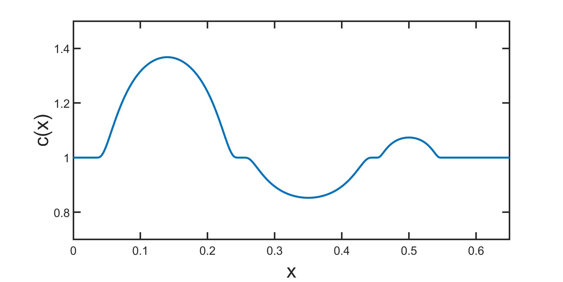
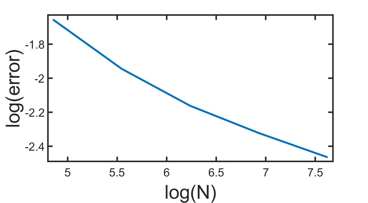
Figure 1. Left: The function $c(x)$ used in computational examples. Right: Convergence of the error (60) as a function of $\mathbb{N}$ in log-log axes.

We use the wave speed function $c$ in Figure 1 in all the computational examples below. It satisfies the bounds (54) with $L_{0}=0.05$, $L_{1}=0.55$, $C_{0}=0.8$ and $C_{1}=1.4$. Moreover, we take $T=2$ and then (55) holds. In the one dimensional case, the travel time metric is given by metric tensor $g=c(x)^{-2}dx^{2}$ and the corresponding distance function $d(x_{1},x_{2})=d_{g}(x_{1},x_{2})$ (i.e., travel time beween points is given by

(56) $$d(x_{1},x_{2})=\int_{x_{1}}^{x_{2}}\frac{1}{c(x)}dx,\quad x_{1}\leq x_{2}.$$

We denote by ${\bf x}(r)$ the point that satisfies $d(0,{\bf x}(r))=r$, that is, ${\bf x}(r)\in M$ is the point which travel time to the boundary point 0 is $r$. The domain of influence for the boundary point $0$ and time $r>0$ are

(57) $$M(r)=\{x\in M;d(0,x)\leq r\}.$$

6.1. Simulation of measurement data

We use $H^{1}$-conformal piecewise affine finite elements on a regular grid on $(0,2T)$ to discretize the Neumann-to-Dirichlet operator $\Lambda$. Let us explain this in more detail. For $\mathbb{N}\in\mathbb{Z}_{+}$ and $n=1,...,2\mathbb{N}-1$ we write $h=T/\mathbb{N}$ and denote by $\phi_{n,\mathbb{N}}\in H_{0}^{1}(0,2T)$ the function that is supported on $[(n-1)h,(n+1)h]$, that satisfies $\phi_{n,\mathbb{N}}(nh)=1$, and whose restrictions on $[(n-1)h,nh]$ and $[nh,(n+1)h]$ are affine. Then the subspace

(58) $$\mathcal{P}^{\mathbb{N}}=\hbox{span}\big{\{}\phi_{1,\mathbb{N}},\dots,\phi_{2\mathbb{N}-1,\mathbb{N}}\big{\}}\subset H^{1}_{0}(0,2T)$$

consists of piecewise affine functions and we write

(59) $$P^{\mathbb{N}}:H^{1}_{0}(0,2T)\to\mathcal{P}^{\mathbb{N}},\quad P^{\mathbb{N}}f(t)=\sum_{j=1}^{2{\mathbb{N}}-1}f(jh)\phi_{j,\mathbb{N}}(t).$$

for the corresponding interpolation operator. The function $u^{\phi_{1,\mathbb{N}}}$, solving (53) with $f=\phi_{1,\mathbb{N}}$, is computed with high accuracy using the $k$-Wave solver [44]. Then we define the discretization of $\Lambda$,

$$\Lambda_{\mathbb{N}}^{(d)}:\mathcal{P}^{\mathbb{N}}\to\mathcal{P}^{\mathbb{N}},$$

by $\Lambda_{\mathbb{N}}^{(d)}\phi_{1,\mathbb{N}}=P^{\mathbb{N}}(u^{\phi_{1,\mathbb{N}}}|_{x=0})$ together with the translation invariance in time, $\Lambda_{\mathbb{N}}^{(d)}\phi_{j,\mathbb{N}}(t)=\Lambda_{\mathbb{N}}^{(d)}\phi_{1,\mathbb{N}}(t-(j-1)h),$ for $j=2,3,\dots,2\mathbb{N}-1$. We can also write

$$\Lambda_{\mathbb{N}}^{(d)}f=\sum_{j=1}^{2\mathbb{N}-1}\sum_{k=1}^{j}f_{k}\Lambda_{j-k+1}\phi_{j,\mathbb{N}},\quad\text{for}\quad f=\sum_{j=1}^{2\mathbb{N}-1}f_{j}\phi_{j,\mathbb{N}}.$$

In the computational examples, $u^{\phi_{1,\mathbb{N}}}$ is solved using a regular mesh with $2^{13}$ spatial and $2^{15}$ temporal cells.

6.2. Implementation of the energy focusing

Computational implementation of the energy focusing method boils down to solving discretized versions of the linear equations (28) and (29).

Most of the operators $X$ appearing in (28) and (29) are simply discretized by setting $X^{(d)}\phi_{j,\mathbb{N}}=P^{\mathbb{N}}X\phi_{j,\mathbb{N}}$. This is the case for $R$ and $J$, see the definition (16) of $K$, as well as, for $N$ and $Q$ in (29).

In the $1+1$-dimensional case, the projection $P$, appearing in (28) and (29), is equal to the multiplication with the characteristic function of the interval $(T-r,T)$ for some $r$, that is,

$$P=P_{r}:L^{2}(0,T)\to L^{2}(0,T),\quad(P_{r}f)(t)=\mathds{1}_{(T-r,r)}(t)f(t).$$

We discretize $P$ by setting

$$P^{(d)}\phi_{j,\mathbb{N}}=\begin{cases}\phi_{j,\mathbb{N}},&T-r<jh<T,\\ 0,&\text{otherwise}.\end{cases}$$

Then $P^{(d)}:\mathcal{P}^{\mathbb{N}}\to\mathcal{P}^{\mathbb{N}}$. The projection $\widehat{P}$ is discretized analogously, see the definition (30) of $L$. The time derivative is discretized using first order forward finite differences at the points $nh$, $n=1,\dots,2\mathbb{N}-2$, as follows

$$\partial_{t}^{(d)}f=\sum_{j=1}^{2\mathbb{N}-2}\frac{f_{j+1}-f_{j}}{h}\phi_{j,\mathbb{N}}(t),\quad\text{for}\quad f=\sum_{j=1}^{2\mathbb{N}-1}f_{j}\phi_{j,\mathbb{N}}.$$

We have now given discretizations of all the operators appearing in (28) and (29). The function $\Phi_{T}$ on the right-hand side of (28) is discretized by $\Phi_{T}^{(d)}=P^{\mathbb{N}}\Phi_{T}$. Solving for $h$ in (28), with the operators replaced by their discretizations, gives us $h_{\alpha}^{(d)}\in\mathcal{P}^{\mathbb{N}}$. Then we solve for $a$ in (29), with the operators replaced again by their discretizations, and with $h_{\alpha}$ replaced by $h_{\alpha}^{(d)}$. We denote the so obtained solution by $a^{(d)}\in\mathcal{P}^{\mathbb{N}}$.

We use the restarted generalized minimal residual (GMRES) method to solve the discrete versions of (28) and (29). The maximum number of outer iterations is 6 and the number of inner iterations (restarts) is 10. We use zero as the initial guess, and the tolerance of the method is set to $10^{-12}$.

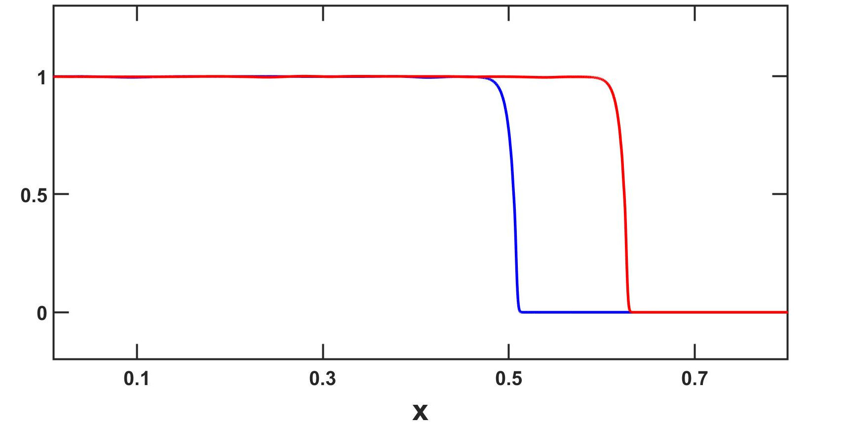
Figure 2. Functions $u^{P_{r_{1}}h_{1}}(x,T)\approx 1_{M(r_{1})}(x)$ (blue) and $u^{P_{r_{2}}h_{2}}(x,T)\approx 1_{M(r_{2})}(x)$ (red), where $h_{1}$ and $h_{2}$ are obtained by solving the discretized version of (28).

6.3. Computational examples

We set $r_{1}=\frac{1}{2}$, $r_{2}=\frac{5}{8}$ and $\mathbb{N}=2^{11}$, and denote by $h_{\alpha,j}^{(d)}$ the solution of the discretized version of (28) with $r=r_{j}$, $j=1,2$. The solutions $u^{P_{r_{1}}h_{\alpha,1}^{(d)}}(x,T)$ and $u^{P_{r_{2}}h_{\alpha,2}^{(d)}}(x,T)$ with $\alpha=0.001$ are shown in Figure 2. Moreover, we denote by $a_{j}^{(d)}$ the solution of the discretized version of (29) with $h_{\alpha}=h_{\alpha,j}^{(d)}$. The difference of the corresponding solutions

$$u^{a_{2}^{(d)}}(x,T)-u^{a_{1}^{(d)}}(x,T)=u^{a_{2}^{(d)}-a_{1}^{(d)}}(x,T),$$

with $\beta=1.02\,\cdotp 10^{-4}$ and $\alpha$ as above, is shown in Figure 3. The spurious oscillations near the origin in Figure 3 were present also in our computations using finer discretizations, however, they appear to converge to zero in $L^{2}(M)$ as predicted by Theorem 1.1. Convergence of the error

(60) $$\|u^{a_{2}^{(d)}-a_{1}^{(d)}}_{t}(\cdot,T)-\mathds{1}_{M(r_{2})\setminus M(r_{1})}\|_{L^{2}(M)}$$

is shown in Figure 1 (Right) as a function of $\mathbb{N}$. Different regularization parameters $\alpha$ and $\beta$ are chosen for each $\mathbb{N}$.

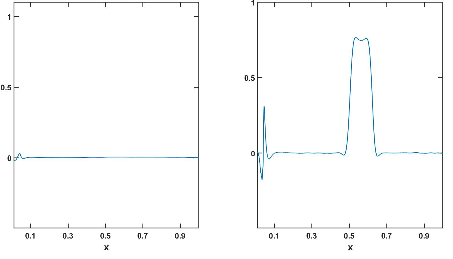
Figure 3. Functions $u^{a}(x,T)$ (left) and $\partial_{t}u^{a}(x,T)$ (right) where $a=a_{2}^{(d)}-a_{1}^{(d)}$ and $a_{1}^{(d)}$ and $a_{2}^{(d)}$ are the solutions to the discretized version of the minimization problem (29). The time derivative of the wave at time $T$, that is, $x\mapsto u^{a}_{t}(x,T)$, where $a=a_{2}^{(d)}-a_{1}^{(d)}$, is concentrated near the interval $[{\bf x}(r_{1}),{\bf x}(r_{2})]=\hbox{cl}({M(r_{2})\setminus M(r_{1})})$, where ${\bf x}(r_{1})\approx 0.5$ and ${\bf x}(r_{2})\approx 0.62.$ The “spike” in the time derivative on right close to the value x = 0.05 has a relatively small $L^{2}$-norm despite its visual appearance.

7. Observation times and boundary distance functions

In this section we will apply focusing of waves to inverse problems, that is, to determine the coefficients of the operator ${\mathcal{A}}$ that correspond to the unknown material functions in $M$. Results in [4, 6, 23] show that the mapping $\Lambda$ determines uniquely the isometry type of the Riemannian manifold $(M,g)$. Here we consider an alternative proof for these results. We show that $\Lambda$ determines the time when the wave emanating from a point source in the domain $M$ is observed at different points of the boundary $\partial M$. We do this by considering waves that focus at a point $\widehat{x}$. As shown in formula (5), the waves focusing at time $T$ to the point $\widehat{x}$ converge to Green’s function $G(x,t,\widehat{x},T)$ at times $t>T$. Below we show that by considering the boundary values of the focusing waves we can determine the observation times from point sources located at all points $\widehat{x}\in M$. These functions determine the metric $g$ in $M$ up to an isometry, see [23]. A similar approach has been used for non-linear wave equation, e.g. $\square_{g}u+au^{2}=0$, where the non-linear interaction of the waves is used to produce artificial microlocal points sources in $M\times{\mathbb{R}}$. Such artificial microlocal points sources determine the information analogous to the observation times from point sources in the medium, see [14, 18, 29, 31]. We note that for genuinely non-linear equations this technique makes it possible to solve inverse problems for non-linear equations that are still unsolved for linear equations, e.g. for equations with a time-varying metric. Below, we will show that some of these techniques are applicable also for linear wave equations.

Consider a manifold $(M,\texttt{g})$ and Green’s function $G(\cdot,\cdot\,;\widehat{x},T)$ satisfying (2). For $\widehat{x}\in M$, $T\in{\mathbb{R}}$, and $y\in\partial M$ we define the observation time function corresponding to a point source at $(\widehat{x},T)\in M\times{\mathbb{R}}$,

$$\mathcal{T}_{\widehat{x},T}(y) = \sup\{t\in{\mathbb{R}};\hbox{ the set $\{y\}\times(-\infty,t)$ has a neighborhood}$$

$$\quad\quad\hbox{ $U\subset\partial M\times{\mathbb{R}}$ such that $G(\cdot,\cdot,\widehat{x},T)\big{|}_{U}=0$}\}.$$

In other words, $\mathcal{T}_{\widehat{x},T}(y)$ is the first time when the wave $G(\cdot,\cdot,\widehat{x},T)$ is observed on the boundary at the point $y$.

Proposition 7.1.

(i) For all $z\in{\partial M}$, the pair $(\partial M,g|_{\partial M})$ and the map $\Lambda$ determines function $\tau_{\partial M}(z)$.

(ii) For all $z\in{\partial M}$ and ${{\widehat{t}}}<\tau_{\partial M}(z)$ the pair $(\partial M,g|_{\partial M})$ and the map $\Lambda$ determines $\mathcal{T}_{x,T}(z)$ for the point $x=\gamma_{z,\nu}({{\widehat{t}}})\in M$.

(iii) We have $\mathcal{T}_{\widehat{x},T}(y)=\texttt{d}_{M}(y,\widehat{x})+T$.

Proof.

Let us first prove (iii), and then (i) and (ii).

(iii) Using the finite velocity of the wave propagation for the wave equation, see [19], we obtain that the support of Green’s function $G(\cdot,\cdot,\widehat{x},T)$ is contained $J^{+}(q)\cap(\partial M\times{\mathbb{R}})$, where $J^{+}(q)$ is in the causal future the point $q=(\widehat{x},T)\in M\times{\mathbb{R}}$, given by

$$J^{+}(q)=\{(y^{\prime},s)\in M\times{\mathbb{R}};\ s\geq\texttt{d}_{M}(y^{\prime},\widehat{x})+T\}.$$

This implies that $G(\cdot,\cdot,\widehat{x},T)=0$ in $J^{+}(q)$ and that $\mathcal{T}_{\widehat{x},T}(y)\geq\texttt{d}_{M}(y,\widehat{x})+T$. Next, we consider the opposite inequality. To this end, assume that there is $t_{1}>\texttt{d}_{M}(y,\widehat{x})+T$ such that $t_{1}<\mathcal{T}_{\widehat{x},T}(y)$. Then, $G(\cdot,\cdot;\widehat{x},T)$ vanishes in an open set $U_{1}\subset\partial M\times{\mathbb{R}}$ that contains $\{y\}\times(-\infty,t_{1})$. As $\partial_{\nu}G(\cdot,\cdot;\widehat{x},T)|_{\partial M\times{\mathbb{R}}}=0$, we then have that the Cauchy data of $G(\cdot,\cdot;\widehat{x},T)$ vanishes in the set $U_{1}$. Let $\psi_{\varepsilon}\in C^{\infty}({\mathbb{R}})$ be a function such that $\int_{\mathbb{R}}\psi_{\varepsilon}(t)dt=1$ and $\hbox{supp }(\psi_{\varepsilon})\subset(-\varepsilon,\varepsilon)$. By the above, the function

$$G^{\varepsilon}(x,t;\widehat{x},T)=\int_{\mathbb{R}}G(x,t-t^{\prime};\widehat{x},T)\psi_{\varepsilon}(t^{\prime})dt^{\prime}$$

is a $C^{\infty}$-smooth function satisfies the homogeneous wave equation

(62) $$\left(\partial^{2}_{t}-\mathcal{A}\right)G^{\varepsilon}(\cdot,\cdot;\widehat{x},T)=0,\quad\hbox{on }(M\times{\mathbb{R}})\setminus I_{\varepsilon},$$

$$G^{\varepsilon}(\cdot,\cdot;\widehat{x},T)|_{U^{\varepsilon}_{1}}=0;\,\,\partial_{\nu}G^{\varepsilon}(\cdot,\cdot;\widehat{x},T)|_{U^{\varepsilon}_{1}}=0$$

where $U^{\varepsilon}_{1}\subset\partial M\times{\mathbb{R}}$ is a neigbhorhood of $\{y\}\times(-\infty,t_{1}-\varepsilon)$ and $I_{\varepsilon}=\{\widehat{x}\}\times(T-\varepsilon,T+\varepsilon).$ Using Tataru’s unique continuation theorem [43] in the domain $M\times{\mathbb{R}}$ we see that

$$G^{\varepsilon}(x,t;\widehat{x},T)=0\quad\hbox{ for }(x,t)\in\{(M\times{\mathbb{R}})\setminus\{\widehat{x}\}\times I_{\varepsilon}):\ t<t_{1}-\texttt{d}_{M}(x,y)-\varepsilon\}.$$

As $G^{\varepsilon}(x,t;\widehat{x},T)\to G(x,t;\widehat{x},T)$ in the domain $(M\setminus\{x_{0}\})\times{\mathbb{R}}$ in sense of distributions as $\varepsilon\to 0$, we see that

$$\hbox{$G(x,t;\widehat{x},T)=0$ for $(x,t)\in\mathcal{V}\setminus\{(\widehat{x},T)\}$},$$

where

$$\mathcal{V}=\{(x,t)\in M\times{\mathbb{R}}:\ t<t_{1}-\texttt{d}_{M}(x,y)\}.$$

Since $\mathcal{V}$ is an open neighborhood of the point $(\widehat{x},T)$, we see that $G(\cdot,\cdot;\widehat{x},T)|_{\mathcal{V}}$ is a distribution supported in a single point $(\widehat{x},T)$. By [41], this implies that $F=G(\cdot,\cdot;\widehat{x},T)|_{\mathcal{V}}$ is finite sum of derivatives of the delta distribution supported at $(\widehat{x},T)$. Considering such a distribution $F$ in local coordinates and computing its Fourier transform, we see that $(\partial_{t}^{2}-\mathcal{A})F$ can not be the delta-distribution $\delta_{(\widehat{x},T)}(x,t)$. This is in contradiction with the equation (2), and hence we conclude that the claimed $t_{1}\in(\texttt{d}_{M}(y,\widehat{x})+T,\mathcal{T}_{\widehat{x},T}(y))$ can not exists. Thus $\mathcal{T}_{\widehat{x},T}(y)=\texttt{d}_{M}(y,\widehat{x})+T$. This proves (iii).

(i) The map $\Lambda$ determines the functions $f_{n}{{(\alpha,\beta}},k)$. If ${{\widehat{t}}}>\tau_{\partial M}(z)$, the limit (47) is zero. If ${{\widehat{t}}}<\tau_{\partial M}(z)$, the considerations in the proof of claim (ii) show that the limit (47) is non-zero. Thus $\Lambda$ determines $\tau_{\partial M}(z)$.

(ii) The claim follows from the definition (7) of $\mathcal{T}_{\widehat{x},{{\widehat{t}}}}(y)$.

∎

By (7.1) the pair $(\partial M,g|_{\partial M})$ and map $\Lambda$ determine the function $\tau_{\partial M}(z)$ for all $z\in{\partial M}$. Those determine also $\mathcal{T}_{x,T}(y)$ and $\texttt{d}_{M}(\widehat{x},y)$, $y\in\partial M$ for the point $x=\gamma_{z,\nu}({{\widehat{t}}})\in M$ where ${{\widehat{t}}}<\tau_{\partial M}(z)$. As the distance function is continuous, we see that when ${{\widehat{t}}}\to t_{1}=\tau_{\partial M}(z)$, we have that $\texttt{d}_{M}(\gamma_{z,\nu}({{\widehat{t}}}),y)\to\texttt{d}_{M}(\gamma_{z,\nu}(t_{1}),y)$. Thus the pair $(\partial M,g|_{\partial M})$ and the map $\Lambda$ determine $\texttt{d}_{M}(x_{0},y)$ for the point $x=\gamma_{z,\nu}({{\widehat{t}}})\in M$ for all ${{\widehat{t}}}\leq\tau_{\partial M}(z)$ and $y\in\partial M$. This implies that the pair $(\partial M,g|_{\partial M})$ and $\Lambda$ determine the collection of boundary distance functions, that is, the set

$$R(M)=\{\texttt{d}_{M}(\widehat{x},\,\cdotp)\in C(\partial M):\ \widehat{x}\in M\}.$$

Further, the set $R(M)$ determines the isometry type of $(M,\texttt{g})$, see [23] (see also generalizations of this result in [33] (see also [21]). Moreover, in the case when $M\subset{\mathbb{R}}^{n}$ and ${\mathcal{A}}=-c(x)^{2}\Delta$ we can determine the Euclidean coordinates of the point $\widehat{x}=\gamma_{z,\nu}(\widehat{t})$ using Cor. 4.3. Hence we can determine vector $\widehat{v}=\lim_{t\to\widehat{t}-}\partial_{t}\gamma_{z,\nu}(t)$ and $c(\widehat{x})=1/\|\widehat{v}\|_{{\mathbb{R}}^{n}}$. This gives an algorithm to determine the unknown wave speed $c(x)$ at all points $x\in M$.

Acknowledgements: The research has been partially supported by EPSRC EP/D065711/1, and Academy of Finland, grants 273979, 284715, 312110.

Appendix A

In this appendix, we show that the Blagovestchenskii identities (15),(17), and the energy identity (34) hold.

A.1. Proof of the Blagovestchenskii identity 1 (15)

We have following version of the Blagovestchenskii identity

$$\int_{M}u^{f}(T)u^{h}(T)\,\mathrm{dV}=\int_{{\partial M}\times[0,2T]}(Kf)(x,t)h(x,t)\,dS(x)dt,$$

where $f,h\in V$. The proof given here is in a slightly different context that the one done e.g. in [23].

Proof.

For boundary value problem

(63) $$\begin{cases}\partial_{t}^{2}u^{f}(x,t)-\mathcal{A}u^{f}(x,t)=0,\quad\hbox{ in }M\times{\mathbb{R}}_{+},\\ u^{f}|_{t=0}=0,\quad u^{f}_{t}|_{t=0}=0,\\ \partial_{\nu}u^{f}|_{\partial M\times{\mathbb{R}}_{+}}=f,\end{cases}$$

let us assume that we have solutions $u^{f}$ and $u^{h}$ with respect to boundary sources $f,h\in V)$. Let us define

$$w(t,s)=\int_{M}u^{f}(t){u^{h}(s)}\,\mathrm{dV}_{\mu}.$$

Integrating by parts, we see that

$$(\partial^{2}_{t}-\partial^{2}_{s})w(t,s)$$

$$= -\int_{M}\big{[}{\mathcal{A}}u^{f}(t){u^{h}(s)}-u^{f}(t){{\mathcal{A}}u^{h}(s)}\big{]}\,\mathrm{dV}_{\mu}(x)$$

$$-\int_{\partial M}\big{[}\partial_{\nu}u^{f}(t)u^{h}(s)-u^{f}(t){\partial_{\nu}u^{h}(s)}\big{]}\,dS_{\texttt{g}}$$

$$= \int_{\partial M}\big{[}(-\partial_{\nu}u^{f}(t)+\eta u^{f}(t))u^{h}(s)-u^{f}(t)(-\partial_{\nu}u^{h}(s)+\eta u^{h}(s))\big{]}\,dS_{\texttt{g}}$$

$$= \int_{\partial M}\big{[}f(t)\Lambda h(s)-\Lambda f(t){h(s)}\big{]}\,dS_{\texttt{g}}.$$

Moreover, as

$$\left.w\right|_{t=0}=\left.w\right|_{s=0}=0,\quad\left.\partial_{t}w\right|_{t=0}=\left.\partial_{s}w\right|_{s=0}=0,$$

we can consider (A.1) as one dimensional wave equation with known right hand side and vanishing initial and boundary data. Solving this initial-boundary value problem, we obtain

(65) $$\int_{M}u^{f}(x,T){u^{h}(x,T)}\,\mathrm{dV}_{\mu}(x)=$$

$$\int_{[0,2T]^{2}}\int_{\partial M}J(t,s)\big{[}f(t){(\Lambda h)(s)}-(\Lambda f)(t){h(s)}\big{]}\,dS_{\texttt{g}}(x)dtds,$$

where $J$ is as defined in (13).

The Schwartz kernel of $\Lambda$ is the Dirichlet boundary value of the Green’s function $G(x,x^{\prime},t-t^{\prime})$ satisfying

(66) $$(\partial_{t}^{2}+{\mathcal{A}})G_{x^{\prime},t^{\prime}}(x,t) =\delta_{x^{\prime}}(x)\delta(t-t^{\prime})\quad\hbox{ in }M\times{\mathbb{R}}_{+},$$

$$G_{x^{\prime},t^{\prime}}|_{t=0}=0, \quad\partial_{t}G_{x^{\prime},t^{\prime}}|_{t=0}=0,\quad B_{\nu,\eta}G_{x^{\prime},t^{\prime}}|_{\partial M\times{\mathbb{R}}_{+}}=0,$$

where $G_{x^{\prime},t^{\prime}}(x,t)=G(x,x^{\prime},t-t^{\prime})$. As

$$G(x,x^{\prime},t-t^{\prime})=G(x^{\prime},x,t-t^{\prime}),$$

we see that $\Lambda^{*}=R\Lambda R$ where $Rf(x,t)=f(x,2T-t)$ is the time reversal map.

Thus, we can rewrite formula (65) in the form

(67) $$\quad\quad\int_{M}u^{f}(x,T){u^{h}(x,T)}\,\mathrm{dV}_{\mu}(x)=\int_{\partial M\times[0,2T]}(Kf)(x,t)\,h(x,t)\,dS_{\texttt{g}}(x)dt$$

where $K$ is defined in (16).

Analyzing (16), we see that the inner product in the left-hand side of (67) can be found by making two measurements, one with the input $f$ and the other with the input $RJf,$ obtained from $f$ by basic operations of the time reversal $R$ and the time filtering $J$. ∎

A.2. Proof of the Blagovestchenskii identity 2 (17)

We have following version of the Blagovestchenskii identity (17)

$$\langle u^{h}(T),1\rangle_{L^{2}(M)}=-\langle h,\Phi_{T}\rangle_{V},$$

where $h\in V$ and $\Phi_{T}$ is as defined in (18).

Proof.

Let us assume that we have solution $u^{h}$ for problem (63) with respect to boundary source $h\in V.$ Let us define

$$I(t) = \int_{M}\left[u^{h}(x,t)\right]\,\mathrm{dV}_{\texttt{g}}(x).$$

Differentiation respect the time gives us

$$\partial_{t}^{2}I(t) = \int_{M}\left[\partial_{t}^{2}u^{h}(x,t)\cdot 1\right]\,\mathrm{dV}_{\texttt{g}}(x).$$

Using the definition of problem (63) we have

$$\partial_{t}^{2}I(t) = \int_{M}\left[\mathcal{A}u^{h}(x,t)\cdot 1\right]\,\mathrm{dV}_{\texttt{g}}(x).$$

Integrating by parts, we see that

$$\partial_{t}^{2}I(t) = \int_{M}\big{[}u^{h}(x,t)\mathcal{A}1\big{]}\,\mathrm{dV}_{\mu}(x)-\int_{\partial M}\big{[}\partial_{\nu}u^{h}(x,t)\cdot 1-u^{h}(x,t)\partial_{\nu}1\big{]}\,dS_{\texttt{g}}(x)$$

Thus

$$\partial_{t}^{2}I(t) = -\int_{\partial M}\big{[}h(x,t)\big{]}\,dS_{\texttt{g}}(x)$$

At time $t=0$ we assumed that initial values $\partial_{t}u(x,0)=0$ and $u(x,0)=0$. Thus we have $I(0)=0$ and $\partial_{t}I(0)=0$. Using this we get

$$I(t) = -\int_{0}^{t}\int_{0}^{t^{\prime}}\int_{\partial M}h(x,t^{\prime\prime})\,dS_{\texttt{g}}(x)dt^{\prime\prime}dt^{\prime}.$$

Let us define

$$J_{t} = \big{\{}(t^{\prime},t^{\prime\prime})|0\leq t^{\prime\prime}\leq t^{\prime}\leq t\big{\}}.$$

Using the indicator function we get

$$I(t) = -\int_{0}^{t}\int_{0}^{t}\int_{\partial M}h(x,t^{\prime\prime})\mathds{1}_{J_{t}}(t^{\prime},t^{\prime\prime})\,dS_{\texttt{g}}(x)dt^{\prime\prime}dt^{\prime}.$$

Then we chance the order of integration gives us

$$I(t) = -\int_{\partial M}\int_{0}^{t}h(x,t^{\prime\prime})\big{[}\int_{0}^{t}\mathds{1}_{J_{t}}(t^{\prime},t^{\prime\prime})dt^{\prime}\big{]}dt^{\prime\prime}\,dS_{\texttt{g}}(x)$$

$$= -\int_{\partial M}\int_{0}^{t}h(x,t^{\prime\prime})\big{[}\int_{t^{\prime\prime}}^{t}1dt^{\prime}\big{]}dt^{\prime\prime}\,dS_{\texttt{g}}(x)$$

$$= -\int_{\partial M}\int_{0}^{t}h(x,t^{\prime\prime})\big{[}t-t^{\prime\prime}\big{]}dt^{\prime\prime}\,dS_{\texttt{g}}(x).$$

For $t=T$ we have

$$I(T) = -\int_{\partial{M}}\int_{0}^{T}h(x,t^{\prime\prime})\big{[}T-t^{\prime\prime}\big{]}dt^{\prime\prime}\,dS_{\texttt{g}}(x).$$

Thus

$$I(T) = -\int_{\partial{M}}\int_{0}^{2T}h(x,t^{\prime\prime})\widehat{P}\big{[}T-t^{\prime\prime}\big{]}dt^{\prime\prime}\,dS_{\texttt{g}}(x)=-\langle h,\Phi_{T}\rangle_{V}.$$

∎

References

- [1] M. Anderson, A. Katsuda, Y. Kurylev, M. Lassas, and M. Taylor. Boundary regularity for the ricci equation, geometric convergence, and gel’fand’s inverse boundary problem. Invent. Math., 158:261–321, 2004.
- [2] G. Bal and L.Ryzhik. Time reversal and refocusing in random media. SIAM J. Appl. Math, 63:1475–1498, 2003.
- [3] G. Bal and O. Pinaud. Time reversal based detection in random media. Inverse Problems, 21:1593–1620, 2005.
- [4] M. Belishev. An approach to multidimensional inverse problems for the wave equation. (russian). Dokl. Akad. Nauk SSSR, 297:524–527, 1987.
- [5] M. Belishev. Wave bases in multidimensional inverse problems. Mathematics of the USSR-Sbornik, 67:584–602, 1990.
- [6] M. Belishev and Y. Kurylev. To the reconstruction of a riemannian manifold via its spectral data (bc-method). Comm. Partial Differential Equations, 17:767–804, 1992.
- [7] K. Bingham, Y. Kurylev, M. Lassas, and S. Siltanen. Iterative time-reversal control for inverse problems. Inverse Problems and Imaging, 2(1), 2008.
- [8] L. Borcea, G. Papanicolaou, and C. Tsogka. Theory and applications of time reversal and interferometric imaging. Inverse Problems, 19:5139–5164, 2003.
- [9] L. Borcea, G. Papanicolaou, C. Tsogka, and J. Berryman. Imaging and time reversal in random media. Inverse Problems, 18:1247–1279, 2002.
- [10] P. Caday, M. V. de Hoop, V. Katsnelson, and G. Uhlmann. Scattering control for the wave equation with unknown wave speed. Arch. Ration. Mech. Anal., 231(1):409–464, 2019.
- [11] M. Cheney, D. Isaacson, and M. Lassas. Optimal acoustic measurements. SIAM J. Appl. Math., 61(5):1628–1647, 2001.
- [12] M. Cheney, D. Isaacson, and J. C. Newell. Electrical impedance tomography. SIAM Rev., 41(1):85–101, 1999.
- [13] M. Dahl, A. Kirpichnikova, and M. Lassas. Focusing waves in unknown media by modified time reversal iteration. SIAM Journal on Control and Optimization, 48:839–858, 2009.
- [14] M. de Hoop, G. Uhlmann, and Y. Wang. Nonlinear interaction of waves in elastodynamics and an inverse problem. Math. Ann., 376(1-2):765–795, 2020.
- [15] A. Feizmohammadi and Y. Kian. Recovery of nonsmooth coefficients appearing in anisotropic wave equations. SIAM J. Math. Anal., 51(6):4953–4976, 2019.
- [16] M. Fink. Time-reversal acoustics in complex environments. Geophysics, 71:SI151–SI164, 2006.
- [17] M. Fink, D. Cassereau, A. Derode, C. Prada, P. Roux, M. Tanter, J.-L. Thomas, and F. Wu. Time-reversed acoustics. Rep. Prog. Phys., 63:1933–1995, 2000.
- [18] P. Hintz and G. Uhlmann. Reconstruction of Lorentzian manifolds from boundary light observation sets. Int. Math. Res. Not. IMRN, (22):6949–6987, 2019.
- [19] L. Hörmander. The analysis of linear partial differential operators. IV. 275. Springer-Verlag, 1985.
- [20] D. Isaacson. Distinguishability of conductivities by electric current computed tomography. IEEE Transactions on Medical Imaging, 5(2):91–95, 1986.
- [21] S. Ivanov. Distance difference representations of riemannian manifolds. Geometriae Dedicata, 207:167–192, 2018.
- [22] B. Jonsson, M. Gustafsson, V. Weston, and M. de Hoop. Retrofocusing of acoustic wave fields by iterated time reversal. SIAM J. Appl. Math., 64:1954–1986, 2014.
- [23] A. Katchalov, Y. Kurylev, and M. Lassas. Inverse boundary spectral problems. Chapman & Hall/CRC, 2001.
- [24] A. Katchalov, Y. Kurylev, M. Lassas, and N. Mandache. Equivalence of time-domain inverse problems and boundary spectral problem. Inverse problems, 20:419–436, 2004.
- [25] A. Katsuda, Y. Kurylev, and M. Lassas. Stability of boundary distance representation and reconstruction of riemannian manifolds. Inverse Problems and Imaging, 1:135–157, 2007.
- [26] Y. Kian, Y. Kurylev, M. Lassas, and L. Oksanen. Unique recovery of lower order coefficients for hyperbolic equations from data on disjoint sets. J. Differential Equations, 267(4):2210–2238, 2019.
- [27] Y. Kian, M. Morancey, and L. Oksanen. Application of the boundary control method to partial data Borg-Levinson inverse spectral problem. Math. Control Relat. Fields, 9(2):289–312, 2019.
- [28] K. Krupchyk and G. Uhlmann. A remark on partial data inverse problems for semilinear elliptic equations. Proc. Amer. Math. Soc., 148(2):681–685, 2020.
- [29] Y. Kurylev, M. Lassas, and G. Uhlmann. Inverse problems for lorentzian manifolds and non-linear hyperbolic equations. Invent. Math., 212(3):781–857, 2018.
- [30] I. Lasiecka and R. Triggiani. Regularity theory of hyperbolic equations with nonhomogeneous neumann boundary conditions. ii. general boundary data. J. Differential Equations, 94:112–164, 1991.
- [31] M. Lassas. Inverse problems for linear and non-linear hyperbolic equations. In Proceedings of the International Congress of Mathematicians—Rio de Janeiro 2018. Vol. IV. Invited lectures, pages 3751–3771. World Sci. Publ., Hackensack, NJ, 2018.
- [32] M. Lassas and L. Oksanen. Inverse problem for the Riemannian wave equation with Dirichlet data and Neumann data on disjoint sets. Duke Math. J., 163(6):1071–1103, 2014.
- [33] M. Lassas and T. Saksala. Distance difference representations of subsets of complete riemannian manifolds. RIMS Kokyuroku, 10(2023):50–68, 2017.
- [34] M. Malinen, T. Huttunen, and J. P. Kaipio. An optimal control approach for ultrasound induced heating. International Journal of Control, 76, 2003.
- [35] T. Mast, A. Nachman, and R. Waag. Focusing and imaging using eigenfunctions of the scattering operator. J. Acoust. Soc. Am., 102:715–725, 1997.
- [36] G. Papanicolaou, L. Ryzhik, and K. Solna. Statistical stability in time reversal. SIAM J. on Appl. Math., 64:1133–1155, 2004.
- [37] C. Prada, J.-L. Thomas, and M. Fink. The iterative time reversal process: Analysis of the convergence. J. Acoust. Soc. Am., 97:62–71, 1995.
- [38] Rakesh. A linearised inverse problem for the wave equation. Comm. Partial Differential Equations, 13(5):573–601, 1988.
- [39] Rakesh. Reconstruction for an inverse problem for the wave equation with constant velocity. Inverse Problems, 6(1):91–98, 1990.
- [40] Rakesh and P. Sacks. Uniqueness for a hyperbolic inverse problem with angular control on the coefficients. J. Inverse Ill-Posed Probl., 19(1):107–126, 2011.
- [41] W. Rudin. Functional analysis. Second edition. McGraw-Hill, Inc., New York, 1991.
- [42] P. Stefanov and G. Uhlmann. Stable determination of generic simple metrics from the hyperbolic Dirichlet-to-Neumann map. Int. Math. Res. Not., (17):1047–1061, 2005.
- [43] D. Tataru. Unique continuation for solutions to pdes, between hörmander’s theorem and holmgren’s theorem. Comm. Part. Diff. Equations, 20:855–884, 1995.
- [44] B. E. Treeby and B. T. Cox. k-Wave: MATLAB toolbox for the simulation and reconstruction of photoacoustic wave fields. Journal of Biomedical Optics, 15(2):1 – 12, 2010.
- [45] G. Uhlmann. Inverse boundary value problems for partial differential equations. In Proceedings of the International Congress of Mathematicians, Vol. III (Berlin, 1998), number Extra Vol. III, pages 77–86, 1998.
- [46] G. Uhlmann. The Cauchy data and the scattering relation. In Geometric methods in inverse problems and PDE control, volume 137 of IMA Vol. Math. Appl., pages 263–287. Springer, New York, 2004.
- [47] Y. Wang and T. Zhou. Inverse problems for quadratic derivative nonlinear wave equations. Comm. Partial Differential Equations, 44(11):1140–1158, 2019.