es
| (1) |
Explainable, Stable, and Scalable Graph Convolutional Networks for Learning Graph Representation
Abstract
The network embedding problem that maps nodes in a graph to vectors in Euclidean space can be very useful for addressing several important tasks on a graph. Recently, graph neural networks (GNNs) have been proposed for solving such a problem. However, most embedding algorithms and GNNs are difficult to interpret and do not scale well to handle millions of nodes. In this paper, we tackle the problem from a new perspective based on the equivalence of three constrained optimization problems: the network embedding problem, the trace maximization problem of the modularity matrix in a sampled graph, and the matrix factorization problem of the modularity matrix in a sampled graph. The optimal solutions to these three problems are the dominant eigenvectors of the modularity matrix. We proposed two algorithms that belong to a special class of graph convolutional networks (GCNs) for solving these problems: (i) Clustering As Feature Embedding GCN (CAFE-GCN) and (ii) sphere-GCN. Both algorithms are stable trace maximization algorithms, and they yield good approximations of dominant eigenvectors. Moreover, there are linear-time implementations for sparse graphs. In addition to solving the network embedding problem, both proposed GCNs are capable of performing dimensionality reduction. Various experiments are conducted to evaluate our proposed GCNs and show that our proposed GCNs outperform almost all the baseline methods. Moreover, CAFE-GCN could be benefited from the labeled data and have tremendous improvements in various performance metrics.
Index Terms:
Graph convolutional networks (GCNs), graph neural networks (GNNs), network embedding, eigenvectors.I Introduction
Network embedding that learns a representation of a graph in a Euclidian space can be very useful for addressing several important problems, including link prediction, community detection (clustering), node classification, and graph classification. As such, it has attracted a lot of attention lately. In [1], the authors provided a very good conceptual review of key advancements in this area of representation learning on graphs. These include matrix factorization-based methods (such as Laplacian Eigenmaps [2], Graph Factorization [3], GraRep [4], and HOPE [5]), random-walk based algorithms (such as DeepWalk [6] and node2vec [7]), and graph neural networks [8, 9]. However, as pointed out in the review paper [1], there are still some open challenges. In particular, most of these network embedding algorithms do not scale well to handle millions of nodes. They are also difficult to interpret the physical meanings of the embedding vectors.
To tackle the scalability problem and the interpretability problem, in this paper, we propose the Clustering As Feature Embedding GCN (CAFE-GCN) algorithm that uses the clustering results to obtain embedding vectors. Our algorithm is based on two of our previous works: (i) the probabilistic framework of sampled graphs, and (ii) the softmax clustering algorithm.
The probabilistic framework of sampled graphs [10, 11]. Given a set of data points (called nodes in the paper) , the embedding problem is to map the data points to vectors in a Euclidean space so that points that are “similar” to each other are mapped to vectors that are close to each other. Such a problem is an ill-posed problem [12] as people might have different views of “similarity” between two points (see, e.g., [13, 14, 15, 1]). In particular, Figure 1 of [1] provides a very insightful illustration for two different views of a character-character interaction graph derived from the Les Misérables novel. To cope with such an ill-posed problem, one needs to specify a “similarity” measure at first. One commonly used “similarity” measure is a bivariate distribution that measures the probability that the two points and are “sampled” together. A set of nodes associated with a bivariate distribution is called a sampled graph in [10, 11]. The probabilistic framework of sampled graphs in [10, 11] defines the notions of (relative) centrality, community, covariance, and modularity that can be interpreted intuitively. More details for the sampling methods, such as the uniform edge sampling, random walk sampling, and PageRank sampling [16], can be found in [10, 11]. One key result of this framework is that community detection (clustering) can be formulated as a modularity maximization problem.
The softmax clustering algorithm [17, 12]. Given a set of data points, the clustering problem is to cluster these data points so that data points within the same cluster are similar to each other and data points in different clusters are dissimilar. Thus, the embedding problem and the clustering problem are closely related [2]. This is a well-known fact and a typical example is the spectral clustering algorithm (see, e.g., [18]) that uses the eigendecomposition to embed data points into a Euclidean space and then uses the -means clustering algorithm to cluster the embedded data points. There are also some previous works that use clustering algorithms for embedding data points (see, e.g., Softmax embedding [17], GraphSAGE-GCN [19], DIFFPOOL[20], Generalized modularity embedding [12] and LouvainNE [21]). As in [17, 12], we use the softmax clustering algorithm to generate the embedding vectors. The key difference is that we take one step further to show that the softmax clustering algorithm is a special form of graph neural networks and the embedding vectors generated this way are actually approximations of dominant eigenvectors of the modularity matrix.
The development of the CAFE-GCN algorithm relies on the following four key insights:
(i) Equivalence of the embedding problem in a sampled graph. We first formulate the embedding problem in a sampled graph as a constrained optimization problem and show that it is equivalent to a trace maximization problem and a matrix factorization problem. The matrix factorization formulation allows us to view the embedding problem in a sampled graph as an autoencoder and solve it by using matrix factorization methods. On the other hand, the trace maximization formulation allows us to view the embedding problem in a sampled graph as a modularity maximization problem and solve it by using well-known modularity maximization algorithms. More importantly, the trace maximization formulation shows that the optimal embedding can be found from the dominant eigenvectors of the modularity matrix (as a result of the Rayleigh-Ritz theorem).
(ii) Softmax clustering as a special form of GCN. The softmax clustering algorithm in [17, 12] is a special case of the Weisfeiler-Lehman (WL) algorithm [22] that assigns the data points to colors (clusters) by using the softmax assignment. As such, it is also a special form of a more general class of graph neural networks [23, 19]. Instead of using the (normalized) Laplacian matrix in the graph convolutional networks (GCNs)[8], CAFE-GCN uses the modularity matrix in the softmax clustering algorithm. The difference between using the Laplacian matrix and the modularity matrix is discussed in detail in Newman’s book [15]. In particular, the Laplacian matrix is more suitable for graph cuts (with a known number of cuts) and the modularity matrix is more suitable for community detection where the number of communities is not known in advance. Moreover, the Laplacian matrix itself is not a “similarity” matrix [24]. Its pseudo-inverse is. But it is very costly to compute the pseudo-inverse of a Laplacian matrix via the eigendecomposition.
(iii) Softmax clustering as a linear-time modularity maximization algorithm. Let be the number of nonzero elements in the bivariate distribution of a sampled graph. Then the computational complexity of the softmax clustering algorithm is for each round of training nodes. If the sampled graph is sparse, i.e., , then the softmax clustering algorithm is a linear-time modularity maximization algorithm that converges monotonically to a local optimum.
(iv) Softmax embedding as approximations of dominant eigenvectors. The dominant eigenvectors of the modularity matrix form the optimal embedding that maximizes the modularity. When is small, one can find the dominant eigenvectors by the power (orthogonal iteration) method (see, e.g., [25]) with computational complexity and memory complexity [26]. When the softmax clustering algorithm converges, it achieves a local maximum of the modularity that partitions the data points into clusters. If the local maximum is very close to the global optimum, then it is possible to find good approximations of the optimal embedding, i.e., the dominant eigenvectors, from the partition. The idea for this is to do one additional step of the orthogonal iteration.
In addition to CAFE-GCN, we propose another GCN, called sphere-GCN, that is also based on a modularity maximization algorithm. As such, the outputs of the sphere-GCN are also approximations of dominant eigenvectors. Like CAFE-GCN, there exists a linear-time implementation when the graph is sparse. The major difference between CAFE-GCN and sphere-GCN is that sphere-GCN embeds data points into a unit sphere, while CAFE-GCN embeds data points into probability vectors.
The contributions of this paper are summarized as follows:
(i) To the best of our knowledge, CAFE-GCN and sphere-GCN are the first scalable, stable, and explainable GCN in the literature. They are linear-time algorithms that output approximations of dominant eigenvectors of the modularity matrix of a sampled graph.
(ii) We conduct a theoretical analysis for CAFE-GCN and derive a theoretical bound between the approximation by CAFE-GCN and the largest eigenvector.
(iii) We show that both CAFE-GCN and sphere-GCN can also be used to solve the dimensionality reduction problem and obtain approximations of the eigenvectors from PCA.
(iv) We also propose a multi-layer CAFE-GCN algorithm that outputs multi-resolution embedding vectors for a sampled graph. The multi-layer CAFE-GCN algorithm is a nearly linear-time algorithm.
(v) By conducting extensive numerical studies, we show that both CAFE-GCN and sphere-GCN are very effective in producing good approximations of dominant eigenvectors. Also, for various experimental settings on the three datasets, Cora [27], Wiki [28], and ego-Facebook [29], our proposed algorithms outperform almost all the baseline methods in the literature, including Graph Factorization [3], DeepWalk [6], node2vec [7], LINE [30], HOPE [5], GraRep [4], and SDNE [31]. In particular, for the node classification task on the Cora dataset [32], the semi-supervised CAFE-GCN achieves almost the same accuracy as the state-of-the-art method without using any side information.
II Equivalence of the embedding problem in sampled graphs
Given a set of data points (called nodes in the paper) , the embedding problem is to map the data points to vectors in a Euclidean space so that points that are “similar” to each other are mapped to vectors that are close to each other. Such a problem is an ill-posed problem and one needs to specify a “similarity” measure at first. One commonly used “similarity” measure is a bivariate distribution that measures the probability that the two points and are “sampled” together. In this paper, we assume that the bivariate distribution is symmetric, i.e.,
| (2) |
A set of nodes associated with a bivariate distribution is called a sampled graph in [10, 11].
Definition 1.
(Covariance, Community, and Modularity [10, 11])) For a sampled graph, the covariance between two nodes and is defined as follows:
| (3) |
Define the modularity matrix be the matrix with its element being (as a generalization of the original modularity matrix in [33]). Moreover, the covariance between two sets and is defined as follows:
| (4) |
Two sets and are said to be positively correlated if . In particular, if a subset of nodes is positively correlated to itself, i.e., , then it is called a community or a cluster. Let , be a partition of , i.e., is an empty set for and . The modularity with respect to the partition , , is defined as
| (5) |
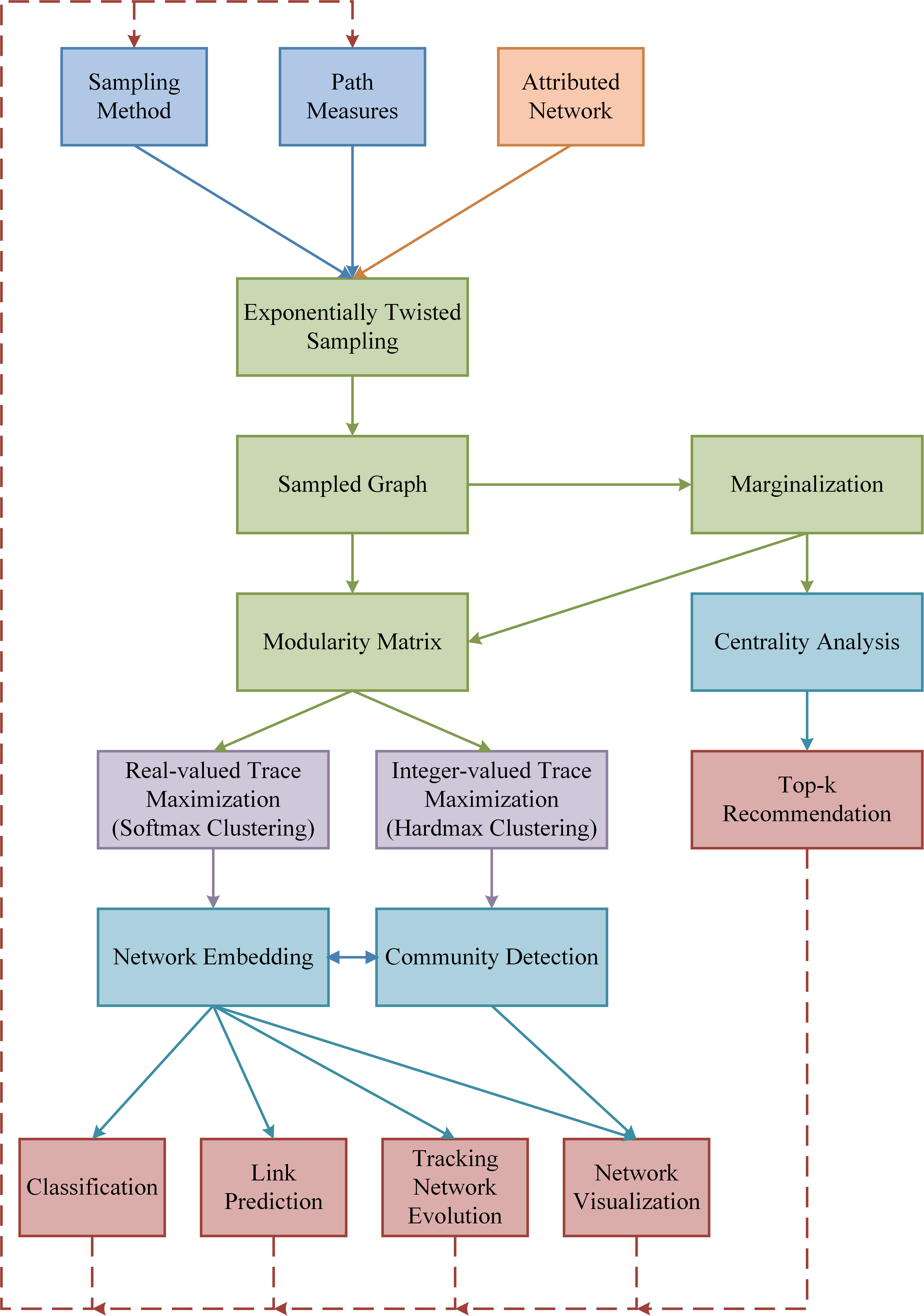
The probabilistic framework was extended to attributed networks in [34], where nodes and edges can have attributes. The idea in [34] is to use exponentially twisted sampling along with path measures that incorporate the information of attributes into sampling. Once sampling is done and a bivariate distribution is obtained, one can then perform centrality analysis, community detection, and network embedding in attributed networks. In Figure 1, we show the dependency graph (flow chart) of various tasks for analyzing attributed networks based on the probabilistic framework. Based on the framework, many tasks, including classification, link prediction, tracking network evolution, network visualization, and top- recommendation, can be developed and written in codes by using sampled graphs as inputs. In particular, community detection (clustering) can be formulated as a modularity maximization problem in [11]. In this paper, we will show that the embedding problem can also be formulated as a modularity maximization problem.
We note that a bivariate distribution can be viewed as a normalized similarity measure. As pointed out in [10], if there is a bounded similarity measure that gives a high score for a pair of two “similar” nodes and , then one can map that similarity measure to a bivariate distribution as follows:
| (6) |
where
| (7) |
is the minimum value of all the similarity scores. The advantage of using bivariate distributions is that we can have probabilistic insights on network analysis. A very interesting recent work on the embedding problem for a bipartite network [35] also used a bivariate distribution to characterize a user-item network. There they showed that the optimal embedding vectors can be interpreted as conditional expectations.
In order to map data points that are similar to each other to vectors that are close to each other, the embedding problem can be formulated as the optimization problem that minimizes the following weighted distance:
| (8) |
where is the vector mapped by node in , and is the squared Euclidean distance between and . To understand the intuition of the minimization problem in (8), note that . Two nodes with a positive (resp. negative) covariance should be mapped to two vectors with a small (resp. large) distance. The embedding vector can be viewed as the “feature” vector of node and is its feature. In practice, it is preferable to have uncorrelated features. For this, we add the constraints
| (9) |
for all . Also, to have bounded values for these features, we also add the constraints
| (10) |
for all .
For such an embedding problem, the following equivalent statements were shown in the book chapter [12].
Theorem 2.
([12], Theorem 3) Let be an symmetric matrix with all its row sums and column sums being , and be the matrix with its row being .
- (i)
- (ii)
From Theorem 2(i), we know that solving the embedding problem is equivalent to solving the trace maximization problem in (11). As stated in [18, 36], a version of the Rayleigh-Ritz theorem shows that the solution of the trace maximization problem in (11) can be found by solving the dominant eigenvectors of the matrix . This is stated in the following corollary.
Corollary 3.
One interpretation of the matrix factorization problem in Theorem 2 is the autoencoder interpretation in [1]. One encodes each row of the modularity matrix into the corresponding row of the matrix and then uses the inner product to decode (and reconstruct an approximation) for the matrix . The error term is known as the loss function.
III The CAFE-GCN algorithm
III-A The softmax clustering algorithm
In [12], a softmax clustering algorithm was proposed for clustering a sampled graph with a symmetric modularity matrix (see Algorithm 1). The softmax clustering algorithm used the softmax function [37] to map a -dimensional vector of arbitrary real values to a -dimensional probability vector. The algorithm starts from a non-uniform probability mass function for the assignment of each node to the clusters. Specifically, let denote the probability that node is in cluster . Then one repeatedly feed each node to the algorithm to learn the probabilities . When node is presented to the algorithm, its expected covariance to cluster is computed for . Instead of assigning node to the cluster with the largest positive covariance (the simple maximum assignment in the literature), Algorithm 1 uses a softmax function to update . Such a softmax update increases (resp. decreases) the confidence of the assignment of node to clusters with positive (resp. negative) covariances. The “training” process is repeated until the objective value converges to a local optimum. The algorithm then outputs the corresponding soft assignment vector for each node. It is worth mentioning that Algorithm 1 can also be used as a semi-supervised learning algorithm. In the case that the clusters (labels) of a certain subset of nodes are known in advance, these nodes will not be affected by the other nodes, and they can be assigned to the corresponding clusters at the beginning of the training process and stay there through the whole training process.
If is a (hard) assignment matrix, then corresponds to a partition of the nodes and is the modularity of that partition. Since is only a soft assignment matrix (with each row being a probability vector), can be viewed as the expected modularity.
The softmax clustering algorithm is in fact a modularity maximization algorithm that increases the expected modularity after each update of the soft assignment matrix. This is stated in the following theorem.
III-B Softmax clustering as a special form of GCN
As mentioned in the previous section, the embedding problem can be solved by finding the dominant eigenvectors of the matrix . When is small, this can be done by the power (orthogonal iteration) method (see, e.g., [25]) with computational complexity and memory complexity [26]. In [26], a fast Chebyshev polynomial approximation algorithm was proposed to avoid the need for eigendecomposition of the matrix , and that motivated Kipf and Welling [8] to propose Graph Convolutional Networks (GCN) for semi-supervised classification. A GCN obtains the embedding vectors by carrying out the following iterations:
| (16) |
where ’s are trainable weight matrices and is an activation function used in a neural network. As such, GCN can be viewed as a special class of graph neural networks (GNNs) in [23]. In this paper, we do not need the trainable weight matrices ’s and they are removed from (16) (or treated as the identity matrix). This leads to the following simplified GCN:
| (17) |
Instead of using the ReLU function in [8], we use the softmax function as our activation function. The softmax function with inputs generate the outputs
| (18) |
where is the inverse temperature. One nice feature of using the softmax function is that now every row of is a probability vector (with all its nonnegative elements summing to ). This leads to a probabilistic explanation of how the GCN in (17) works. Let
| (19) |
be the transpose of the row of the matrix . As pointed out in [8], one can view the GCN as a special case of the Weisfeiler-Lehman (WL) algorithm [22] that assigns the nodes to colors (or clusters). The probability then represents the probability that the node is assigned with color . The GCN starts from a non-uniform probability mass function for the assignment of each node to the colors. Then we repeatedly feed each node to the GCN to learn the probabilities ’s. When node is presented to the GCN, its expected covariance
| (20) |
to color is computed for . Instead of assigning node to the color with the largest positive covariance (the simple maximum assignment), GCN uses a softmax function to update ’s. Such a softmax update increases (resp. decreases) the confidence of the assignment of node to colors with positive (resp. negative) covariances. The “training” process is repeated until it converges.
III-C Softmax clustering as a linear-time modularity maximization algorithm
Let be the number of nonzero elements in the bivariate distribution of a sampled graph. We say a sampled graph is sparse if . Though Algorithm 1 appears to be a matrix-based method, there is a linear-time implementation for a sparse sampled graph by using the techniques outlined in Section IV.B and IV.C of [11]. To see this, note that the modularity matrix (though not sparse) can be decomposed as the difference of a sparse matrix and a rank matrix. Since the updates in (20) are only made locally (with ), the computational complexity of the softmax clustering algorithm is for each round of training nodes. As such, for a sparse sampled graph, the softmax clustering algorithm is a linear-time modularity maximization algorithm that converges monotonically to a local optimum.
III-D Softmax embedding as approximations of dominant eigenvectors
In view of Theorem 4, the sequential implementation of the GCN in (17) outputs a soft assignment matrix that achieves a local optimum of . If we carry out one step of the orthogonal iteration, then we should be able to obtain an orthogonal matrix that is closer to the optimal embedding for the trace maximization problem in Theorem 2(i). Specifically, we compute the QR decomposition for the matrix to find an matrix and an upper triangular matrix so that . Now the matrix is an orthogonal matrix that satisfies the constraint . As shown in Corollary 3, the columns of the optimal embedding matrix are the eigenvectors corresponding to the largest eigenvalues. The matrix is then an approximation of the eigenvectors corresponding to the largest eigenvalues. The detailed steps for obtaining the matrix are shown in the CAFE-GCN algorithm in Algorithm 2.
Similar to Algorithm 1, Algorithm 2 can also be used as a semi-supervised learning algorithm, denoted by CAFE-GCN (semi-supervised) in our experiments in Section VI, when there is a subset of known labels. In the extreme case that all the labels are known, we even do not need to perform the softmax clustering algorithm in Steps (1) and (2). As such, we can go directly to the QR decomposition in Step (3) of Algorithm 2. That leads to a speedy method of obtaining the embedding vectors for a dataset with known labels. Such an algorithm is denoted by CAFE-GCN (full label) in our experiments in Section VI.
III-E Theoretical bounds and numerical results for CAFE-GCN with
In this section, we conduct a theoretical analysis for CAFE-GCN with and derive a theoretical bound between the approximation by CAFE-GCN and the largest eigenvector.
For , we have for all (as each embedding vector is a probability vector). Using this in (15) yields
| (21) |
where we use the assumption that all the row sums and column sums of the matrix are equal to . As a result of Theorem 4 and Theorem 2, the CAFE-GCN with obtains a local optimum solution for the one-dimensional trace maximization in (11). This implies that
should be very close to the largest eigenvalue of the matrix . This motivates us to consider the -vector , where
| (22) |
Now we show that in (22) is close to the eigenvector corresponding to the largest eigenvalue of . Recall that is a symmetric matrix with all its row sums and column sums being . It is well-known that a real symmetric matrix is diagonalizable by an orthogonal matrix. Specifically, let
be the (ordered) eigenvalues of and be the normalized (column) eigenvector corresponding to the eigenvalue , . Let be the orthogonal matrix formed by grouping the eigenvectors together. Then
| (23) |
where is diagonal matrix with the diagonal elements, .
For our analysis, we also assume that there is a spectral gap between the largest eigenvalue and the second-largest eigenvalue magnitude (SLEM), i.e., . Since has an eigenvalue with the eigenvector (with all its elements being ), we know from the spectral gap assumption that . Moreover, as two eigenvectors corresponding two different eigenvalues are orthogonal for a real symmetric matrix, we then have .
To measure the difference between two vectors, we use the cosine similarity defined below.
Definition 5.
The cosine similarity between two -vectors and , denoted by , is
| (24) |
In particular, if both and are unit vectors, i.e., , then the Euclidean distance between these two vectors is
As such, if the cosine similarity between two unit vectors is close to , then the Euclidean distance between these two unit vectors is close to .
In the following theorem, we show a lower bound for the cosine similarity between the vector in (22) and . Its proof is given in Appendix A of this paper.
Theorem 6.
Let the ratio of the SLEM to the largest eigenvalue of , i.e.,
| (25) |
Consider the vector in (22). If
| (26) |
for some satisfying
| (27) |
then
| (28) |
Moreover, and
| (29) |
Theorem 6 shows that if the CAFE-GCN obtains a good solution for the trace maximization problem in the sense of (26) and (27), then it is close to the dominant eigenvector in terms of the bound of the cosine similarity in (28). Moreover, the vector is even closer to , and it is even a better approximation of .
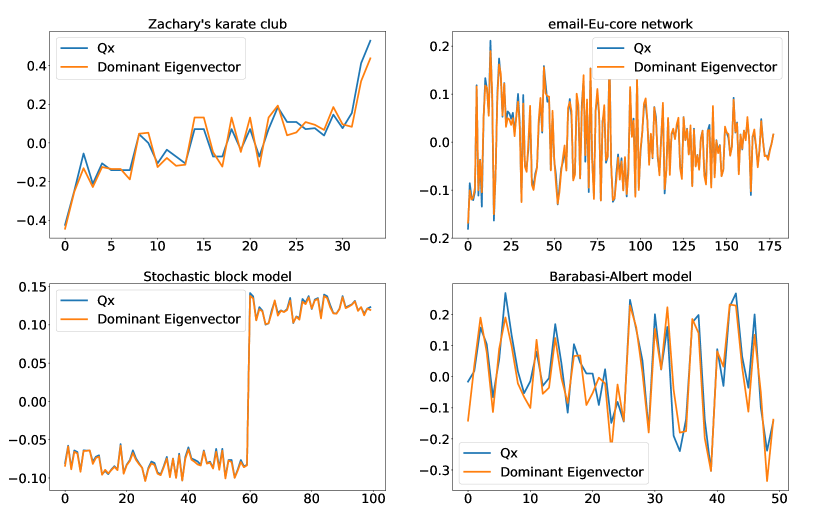
In Figure 2, we show the dominant eigenvector and the unit vector of for four different datasets. These four datasets include two synthetic datasets (a stochastic block model with two blocks [38] and a Barabási–Albert (BA) model [39]), and two real-world datasets (the Zachary’s karate club dataset [40] and the email-Eu-core dataset [41]). Note that we only use the subgraph in the top two communities of the email-Eu-core dataset in this figure. As shown in Figure 2, the differences are very small and the CAFE-GCN indeed computes good approximations of the dominant eigenvectors.
III-F Using the CAFE-GCN for dimensionality reduction
In this section, we show how one can use the CAFE-GCN for the dimensionality reduction problem. Suppose that the data points are in . Let . Assume that the set of points has zero-mean, i.e., for all ,
Note that if the set of data points do not have zero-mean, one can subtract its centroid to make it zero-mean, i.e., the -vector with
Now we represent these data points by an matrix with the row of being . Consider the covariance matrix . Then is an symmetric matrix with zero row sums and column sums. Moreover, it was shown in [12] that is an modularity matrix with the bivariate distribution
when is very small. One widely used method for dimensionality reduction is the principal component analysis (PCA) that finds the eigenvectors corresponding to the largest eigenvalues of . Here we show that one can also use the CAFE-GCN in Algorithm 2 to obtain an embedding matrix for the approximations of the eigenvectors from PCA. Note that the row of is the embedding -vector for .
Let . Then we can rewrite (17) as follows:
| (30) |
Multiplying both side of (30) by yields
| (31) | |||||
where is a function with two input matrices: an matrix and matrix . This leads to an iterative way to find the weight matrices .
Now we give the physical meaning for the matrix when the CAFE-GCN converges. Let be the column of , i.e.,
Suppose that when the CAFE-GCN converges, the matrix is a partition matrix (see Step (9) of Algorithm 2), i.e., every row of contains exactly one and the rest elements are . Let be the column of , and be the set of rows in that have value , i.e., the set of nodes that are assigned to the cluster. Since , we have
This shows that is in line with the centroid of the set of nodes in . As the row of is the embedding -vector for , the element of that embedding vector is simply the inner product of and (before the QR decomposition).
Such an interpretation is in line with the explanation of why Convolutional Neural Networks (CNN) work in the two seminal papers [42, 43]. One key insight in [42, 43] is that a CNN can be decomposed into two stages of subnetworks: the feature extraction (FE) subnet and the decision-making (DM) subnet. The FE subnet in the first stage conducts clustering and produces a new representation of a data point through a sequence of RECOS transforms in [43]. The DM subnet in the second stage then classifies the new representations according to decision labels. As such, a CNN basically performs two tasks: clustering in the first stage and classification in the second stage. As pointed out in [43], the classification part in the second stage is similar to the multilayer perceptrons (MLPs) introduced by Rosenblatt in [44], and this in general only requires a small number of layers. On the other hand, the clustering part in the first stage requires stacking more layers of RECOS transforms and it is less understood how it works. Similarly, one can also decompose a GCN into two stages of subnetworks: the feature extraction subnet and the decision-making subnet. Our CAFE-GCN basically explains the clustering part in the first stage. One key difference between [43] and CAFE-GCN is that the -means clustering is used in [43] while the softmax clustering is used in CAFE-GCN. The -means clustering requires knowing the number of clusters while the softmax clustering, as a modularity maximization algorithm, does not require the number of clusters in advance.
To show the effectiveness of Algorithm 2, we compare the embedding vectors from Algorithm 2 with the eigenvectors from PCA. Let be the column of the output matrix from Algorithm 2 and be the eigenvector corresponding to of . We compute the projection of onto the subspace spanned by , denoted by , as follows:
| (32) |
where is the inner product of and . Note that
| (33) |
If is very close to , then we know that is very close to and thus is very close to .
IV The multi-layer CAFE-GCN
One can further stack multiple CAFE-GCNs together to form a multi-layer CAFE-GCN. By doing so, we can extract multi-resolution features of the dataset. Our approach is based on the fast unfolding algorithm in [11] that serves a multi-resolution clustering algorithm. The fast unfolding algorithm in [11] is a generalization of the Louvain algorithm [45] that recursively merges nodes in clusters into supernodes to form a coarsened graph. Such a step is known as graph coarsening in [1]. LouvainNE [21] uses the Louvain algorithm for node embedding. The differences between LouvainNE and the multi-layer CAFE-GCN are in two aspects: (i) the pooling step that defines how the edge weights of the coarsened graph are specified, and (ii) the embedding step that specifies how the embedding vectors are obtained from the clustering results. As mentioned in the previous section, the embedding step in CAFE-GCN can be interpreted as a step to generate good approximations of the dominant eigenvectors. However, there is no physical interpretation of the embedding from LouvainNE. In the pooling step, the bivariate distribution characterization in [11] provides a natural way to generate the new bivariate distribution of the coarsened graph. On the other hand, there is no explanation for LouvainNE on how the edge weights should be generated for the coarsened graph (and the authors defer that as a future work). The two steps of graph coarsening and pooling as described for the multi-layer CAFE-GCN are described as follows:
Graph coarsening. Instead of using the softmax assignment, one can use the hardmax assignment in Algorithm 2. The matrix now is a partition matrix with each row indicating the cluster of the corresponding node. Let , , be the set of nodes of cluster . Aggregate the nodes in into a supernode . Now we have a new dataset of nodes .
Pooling. For the new dataset, we use the “inherited” bivariate distribution as the pooling operator:
| (34) |
This yields a new modularity matrix as follows:
| (35) |
Then we use the new modularity matrix for the input of the next layer. The detailed steps for the multi-layer CAFE-GCN are outlined in Algorithm 3.
Though there are several recent advances in GCN that use hierarchical clustering algorithm for learning multi-resolution features of graphs (see, e.g., GraphSAGE-GCN [19], DIFFPOOL[20], and LouvainNE [21]), the fast unfolding algorithm in [11] has the following advantages:
- (i)
-
Scalability: Let be the number of nonzero elements in the bivariate distribution of the sampled graph. If the sampled graph is sparse, i.e., , then the computational complexity of the fast unfolding algorithm is for each round of training nodes in a layer. Though the number of layers is in general unknown, it is conjectured to be [11]. Thus, it is a nearly-linear time algorithm.
- (ii)
-
Stability: the fast unfolding algorithm in [11] is a modularity maximization algorithm that increases the modularity after each training. As such, the algorithm is stable as it is guaranteed to converge after a finite number of updates.
- (iii)
-
Interpretability: the embedding vectors at each layer are approximations of dominant eigenvectors of the modularity matrix in that layer.
V The sphere-GCN algorithm
In this section, we propose another network embedding algorithm, called the sphere-GCN algorithm. Like the CAFE-GCN algorithm, the sphere-GCN algorithm is also a trace maximization algorithm that maximizes the modularity of the matrix . The key difference between these two algorithms is the space of embedding vectors. Instead of mapping each embedding vector into a probability vector through the softmax function in the CAFE-GCN algorithm, we map each embedding vector by renormalizing it into a high-dimensional sphere in the sphere-GCN algorithm. The detailed steps for obtaining the embedding vectors are shown in Algorithm 4. For the sphere-GCN algorithm, we show in the following theorem that it also converges monotonically to a local optimum of the trace maximization problem. The proof of Theorem 7 is given in Appendix B.
VI Experimental Results
In this section, we evaluate our proposed GCN Algorithms on several real-world datasets. The experimental results demonstrate that our methods outperform several well-known based-line methods for both the node classification task and the link prediction task. Also, we show that CAFE-GCN is capable of performing dimensionality reduction.
VI-A Datasets
In this subsection, we first introduce the datasets used in the node classification task and the link prediction task. Three real-world datasets are used, which are Cora, Wiki, and ego-Facebook. The detailed descriptions of the datasets are listed as follows.
-
•
Cora[27]: The Cora dataset is a citation network that contains machine-learning papers as nodes and they are classified into seven classes. The Cora dataset consists of edges. The edges between two nodes are the citation links.
-
•
Wiki[28]: The Wiki dataset contains nodes and edges from classes. The nodes represent the Wikipedia articles, and the edges represent the web links between them.
-
•
ego-Facebook[29]: This Facebook dataset was collected from survey participants using the Facebook application developed by [29]. This dataset consists of ego-networks and circles with nodes and edges. Each node might be in multiple circles. Such circles include common universities, sports teams, relatives, etc. For our experiments, we delete multiple edges, self-loops, and nodes that are not in the largest component of the network, and assign each node only to the largest circle. By doing so, we have nodes and edges left in the network. Moreover, each node now belongs to exactly one of the circles left in the network.
VI-B Baseline methods
For both node classification and link prediction, we compare the performance of the proposed GCNs with the following baseline methods:
-
•
Graph Factorization [3]: Graph Factorization uses an approximate factorization of a node similarity matrix (based on the adjacency matrix). As such, Graph Factorization preserves the first-order proximity between nodes.
- •
-
•
node2vec [7]: node2vec also uses the same concept as DeepWalk [6]. The critical difference between node2vec and DeepWalk is that node2vec performs a bias random walk that allows a more flexible definition of a random walk. However, a review paper [47] shows that the biased random walks of node2vec do not have any significant gains for graphs with low clustering coefficient and low reciprocity.
-
•
Large-scale information network embeddings (LINE) [30]: LINE was proposed for embedding a large scale network to preserve the first-order and second-order proximity between nodes.
-
•
High-order Proximity Preserved Embedding (HOPE) [5]: HOPE uses the general similarity measures (such as the Katz measure [48], the rooted PageRank [49] etc.) to quantify asymmetric high-orders proximity between nodes and learns the node embeddings by solving the matrix factorization problem with the generalized Singular Value Decomposition (SVD) [50].
-
•
GraRep [4]: GraRep computes the power of the adjacency matrix in order to capture the -order proximity between nodes and uses matrix factorization techniques to construct the global representations for nodes.
- •
VI-C Network node classification
For the node classification task, every node in the training set is assigned with one label. The task is to predict the labels of the nodes in the testing set by using a classifier trained from the node embedding vectors in the training set and their corresponding labels. The embedding vectors of the nodes in the testing set are then put into the classifier to produce the predicted labels.
In Table I, we show the comparison results of the node classification task. The classifier we use in this task is a well-known classifier, called XGBoost [51]. We use accuracy, score, and area under the receiver operating characteristic curve (ROC AUC) as benchmarks. All the metrics are computed over experiments. Note that, as there exist three clusters that only contain one node in the ego-facebook dataset, the ROC AUC score is not defined in that case. We evaluate all the embedding methods using various fractions of the datasets as the training sets of the classifier (, , and as shown in the second row of Table I). As the embedding dimensions of the CAFE-GCN algorithm are determined by itself, all the other baseline methods use the same embedding dimensions as CAFE-GCN (so that the comparisons could be fair). Moreover, the embedding dimensions of the multi-layer CAFE-GCN and the semi-supervised CAFE-GCN are determined by the algorithms themselves. For each dataset, only semi-supervised CAFE-GCN use labels for embedding. Labels used in semi-supervised CAFE-GCN (marked with CAFE-GCN (semi-supervised) in Table I) are the same as those used in the classifiers. Moreover, all labels are used in CAFE-GCN (full label) in Table I. Also, the best scores of accuracy, scores, and ROC AUC scores are marked in bold.
| Node classification | ||||||||||
| Datasets | Methods / Metrics | 10% Training data | 30% Training data | 50% Training data | ||||||
| Accuracy | AUC | Accuracy | AUC | Accuracy | AUC | |||||
| Cora | Graph Factorization | 0.3530.013 | 0.2810.018 | 0.5800.009 | 0.4610.013 | 0.4000.017 | 0.6410.009 | 0.5140.016 | 0.4600.018 | 0.6730.010 |
| DeepWalk | 0.6710.016 | 0.6420.019 | 0.7860.011 | 0.7730.012 | 0.7550.013 | 0.8500.008 | 0.8080.009 | 0.7930.010 | 0.8740.006 | |
| node2vec | 0.6950.016 | 0.6650.020 | 0.8000.013 | 0.7750.010 | 0.7570.012 | 0.8530.008 | 0.8040.011 | 0.7890.012 | 0.8720.007 | |
| LINE | 0.3040.013 | 0.2290.013 | 0.5510.007 | 0.3650.009 | 0.2880.013 | 0.5810.007 | 0.3950.013 | 0.3190.016 | 0.5960.008 | |
| HOPE | 0.6520.014 | 0.6260.017 | 0.7770.010 | 0.7170.010 | 0.6990.012 | 0.8190.007 | 0.7410.010 | 0.7250.011 | 0.8340.007 | |
| GraRep | 0.6950.013 | 0.6740.016 | 0.8060.010 | 0.7540.009 | 0.7400.010 | 0.8440.006 | 0.7730.010 | 0.7610.011 | 0.8560.007 | |
| SDNE | 0.3100.013 | 0.2490.015 | 0.5620.008 | 0.3630.009 | 0.3030.010 | 0.5890.006 | 0.3890.011 | 0.3300.013 | 0.6030.007 | |
| CAFE-GCN | 0.6390.015 | 0.6090.017 | 0.7730.010 | 0.7010.010 | 0.6770.011 | 0.8100.007 | 0.7230.011 | 0.6990.011 | 0.8230.007 | |
| Mutli-layer CAFE-GCN | 0.6500.014 | 0.6220.020 | 0.7800.011 | 0.7140.010 | 0.6900.011 | 0.8180.007 | 0.7410.011 | 0.7180.011 | 0.8340.007 | |
| Sphere-GCN | 0.7350.014 | 0.7130.017 | 0.8290.011 | 0.7860.008 | 0.7690.010 | 0.8620.006 | 0.8090.010 | 0.7950.011 | 0.8780.007 | |
| CAFE-GCN (semi-supervised) | 0.8670.008 | 0.8560.010 | 0.9180.007 | 0.8770.006 | 0.8680.007 | 0.9240.004 | 0.8810.007 | 0.8720.007 | 0.9260.004 | |
| CAFE-GCN (full label) | 0.8720.007 | 0.8620.008 | 0.9210.005 | 0.8790.005 | 0.8710.006 | 0.9250.004 | 0.8830.007 | 0.8740.007 | 0.9270.004 | |
| Wiki | Graph Factorization | 0.2480.014 | 0.1610.013 | 0.5560.007 | 0.3500.009 | 0.2490.011 | 0.5990.006 | 0.3960.012 | 0.2870.011 | 0.6180.006 |
| DeepWalk | 0.4560.016 | 0.3280.017 | 0.6450.009 | 0.5690.010 | 0.4380.017 | 0.6970.007 | 0.6090.011 | 0.4800.020 | 0.7170.009 | |
| node2vec | 0.4660.015 | 0.3340.016 | 0.6490.009 | 0.5630.010 | 0.4300.015 | 0.6950.007 | 0.5960.013 | 0.4670.020 | 0.7120.010 | |
| LINE | 0.3070.014 | 0.2240.012 | 0.5870.006 | 0.3880.010 | 0.2850.009 | 0.6170.005 | 0.4190.012 | 0.3090.011 | 0.6280.006 | |
| HOPE | 0.4470.016 | 0.3270.014 | 0.6440.007 | 0.5300.011 | 0.3920.010 | 0.6760.005 | 0.5530.010 | 0.4130.011 | 0.6870.005 | |
| GraRep | 0.5120.015 | 0.3730.014 | 0.6700.008 | 0.5880.009 | 0.4430.013 | 0.7030.006 | 0.6120.012 | 0.4690.016 | 0.7160.007 | |
| SDNE | 0.2810.013 | 0.2050.014 | 0.5780.006 | 0.3560.010 | 0.2670.010 | 0.6070.005 | 0.3870.012 | 0.2950.012 | 0.6200.005 | |
| CAFE-GCN | 0.4470.015 | 0.3230.013 | 0.6450.008 | 0.5150.010 | 0.3810.013 | 0.6730.006 | 0.5390.012 | 0.4030.014 | 0.6830.007 | |
| Mutli-layer CAFE-GCN | 0.4500.015 | 0.3240.014 | 0.6430.007 | 0.5220.011 | 0.3830.012 | 0.6710.006 | 0.5460.011 | 0.4040.013 | 0.6820.006 | |
| Sphere-GCN | 0.5410.014 | 0.3940.018 | 0.6810.009 | 0.6170.011 | 0.4800.017 | 0.7210.008 | 0.6440.011 | 0.5180.019 | 0.7370.008 | |
| CAFE-GCN (semi-supervised) | 0.5550.012 | 0.4090.016 | 0.6910.008 | 0.6580.009 | 0.5590.019 | 0.7650.012 | 0.7060.010 | 0.6440.020 | 0.8100.012 | |
| CAFE-GCN (full label) | 0.7280.012 | 0.6000.026 | 0.7890.013 | 0.7660.008 | 0.6970.026 | 0.8380.015 | 0.7770.011 | 0.7250.025 | 0.8520.014 | |
| ego-Facebook | Graph Factorization | 0.3790.011 | 0.1060.007 | N/A | 0.4390.011 | 0.1450.009 | N/A | 0.4660.011 | 0.1610.008 | N/A |
| DeepWalk | 0.6110.015 | 0.2200.016 | N/A | 0.6790.010 | 0.2900.014 | N/A | 0.7030.011 | 0.3140.016 | N/A | |
| node2vec | 0.5930.016 | 0.2140.016 | N/A | 0.6620.011 | 0.2780.011 | N/A | 0.6830.011 | 0.3020.014 | N/A | |
| LINE | 0.4940.013 | 0.1550.009 | N/A | 0.5430.009 | 0.1940.009 | N/A | 0.5620.010 | 0.2120.011 | N/A | |
| HOPE | 0.5260.013 | 0.1750.010 | N/A | 0.5880.011 | 0.2250.011 | N/A | 0.6130.013 | 0.2490.015 | N/A | |
| GraRep | 0.5400.013 | 0.1830.011 | N/A | 0.6050.009 | 0.2410.011 | N/A | 0.6300.012 | 0.2680.015 | N/A | |
| SDNE | 0.5100.014 | 0.1720.012 | N/A | 0.5800.010 | 0.2330.011 | N/A | 0.6060.009 | 0.2590.011 | N/A | |
| CAFE-GCN | 0.5580.015 | 0.2020.013 | N/A | 0.6510.011 | 0.2790.015 | N/A | 0.6830.011 | 0.3080.017 | N/A | |
| Mutli-layer CAFE-GCN | 0.5660.015 | 0.2030.014 | N/A | 0.6520.010 | 0.2800.016 | N/A | 0.6840.010 | 0.3100.016 | N/A | |
| Sphere-GCN | 0.5810.015 | 0.2160.016 | N/A | 0.6750.011 | 0.3000.017 | N/A | 0.7070.009 | 0.3350.018 | N/A | |
| CAFE-GCN (semi-supervised) | 0.6290.013 | 0.2380.016 | N/A | 0.7070.009 | 0.3260.018 | N/A | 0.7340.009 | 0.3600.019 | N/A | |
| CAFE-GCN (full label) | 0.6810.015 | 0.2750.018 | N/A | 0.7280.009 | 0.3440.014 | N/A | 0.7430.010 | 0.3740.021 | N/A | |
As shown in Table I, the proposed sphere-GCN has the best performance for (almost) all the experimental settings. Although DeepWalk is slightly better than sphere-GCN in the ego-facebook dataset when the ratio of the training set is low, the differences in the metrics between the two algorithms are rather small.
CAFE-GCN also has good performance for many experimental settings. Although both the CAFE-GCN and the sphere-GCN maximize the modularity to obtain approximations of the top eigenvectors, the performance of CAFE-GCN is not as good as sphere-GCN. The reason is that the embedding vectors of CAFE-GCN are only composed of positive numbers, and that might leads to different convergence results of (11). However, Table I also shows that CAFE-GCN (semi-supervised) could be benefited from the labeled data and have tremendous improvements in various metrics. Moreover, Table II demonstrates that CAFE-GCN (semi-supervised) could even be as effective as the SplineCNN [52], which is the state-of-the-art method for node classification on the Cora dataset [32] without using additional side information like node attributes. The accuracy of the SplineCNN is directly based on the original paper [52], and all the experimental settings are the same as those in [52], i.e., nodes for training and nodes for testing.
| Node classification on Cora dataset | ||||
| Metric / Method | SplineCNN |
|
||
| Accuracy | 89.48 0.31 | 89.42 1.03 | ||
VI-D Network link prediction
For the link prediction task, we aim to predict whether there is an edge between two nodes. We treat this task as a binary classification problem. We concatenate the two embedding vectors of a pair of two nodes as a data point. If there exists an edge between two nodes, the data point obtained by the concatenation of the two embedding vectors is labeled as . Otherwise, it is labeled as . We also use XGBoost [51] as the classifier and adopt accuracy and score as our benchmarks. All the metrics are computed over experiments. We evaluate all the embedding methods using various fractions of the datasets as the training sets. The results of the link prediction task are shown in Table III. The percentages in the second row of Table III are the fractions of data for the training set of the classifier. Also, the best scores of accuracy and scores are marked in bold.
| Link prediction | |||||||
| Datasets | Methods / Metrics | 10% Training data | 30% Training data | 50% Training data | |||
| Accuracy | F1 | Accuracy | F1 | Accuracy | F1 | ||
| Cora | Graph Factorization | 0.7090.021 | 0.7210.015 | 0.7590.026 | 0.7790.021 | 0.7590.028 | 0.7830.023 |
| DeepWalk | 0.7380.034 | 0.7730.022 | 0.7510.027 | 0.7880.017 | 0.7550.027 | 0.7920.018 | |
| node2vec | 0.8060.030 | 0.8280.023 | 0.8120.030 | 0.8240.024 | 0.8200.032 | 0.8380.026 | |
| LINE | 0.6640.008 | 0.6500.013 | 0.6920.009 | 0.6980.009 | 0.6970.009 | 0.7070.008 | |
| HOPE | 0.8400.020 | 0.8420.020 | 0.8680.022 | 0.8730.019 | 0.8720.020 | 0.8800.015 | |
| GraRep | 0.7010.034 | 0.7260.028 | 0.7050.024 | 0.7390.019 | 0.7150.031 | 0.7510.025 | |
| SDNE | 0.6920.004 | 0.6770.007 | 0.7060.005 | 0.7030.005 | 0.7140.004 | 0.7140.005 | |
| CAFE-GCN | 0.8030.015 | 0.8130.013 | 0.8090.011 | 0.8140.011 | 0.8100.014 | 0.8160.013 | |
| Mutli-layer CAFE-GCN | 0.8020.015 | 0.8130.013 | 0.8100.015 | 0.8130.015 | 0.8120.012 | 0.8190.012 | |
| Sphere-GCN | 0.8840.011 | 0.8820.012 | 0.9050.010 | 0.9040.010 | 0.9120.009 | 0.9120.009 | |
| Wiki | Graph Factorization | 0.7430.016 | 0.6820.016 | 0.7720.014 | 0.7140.015 | 0.7830.010 | 0.7230.013 |
| DeepWalk | 0.7320.029 | 0.7190.022 | 0.7380.030 | 0.7280.022 | 0.7390.028 | 0.7290.021 | |
| node2vec | 0.7730.027 | 0.7420.023 | 0.7920.024 | 0.7640.021 | 0.7940.023 | 0.7660.021 | |
| LINE | 0.8030.004 | 0.7480.005 | 0.8110.003 | 0.7620.004 | 0.8130.003 | 0.7650.004 | |
| HOPE | 0.8350.005 | 0.7780.007 | 0.8440.004 | 0.7910.005 | 0.8450.004 | 0.7930.006 | |
| GraRep | 0.7910.026 | 0.7530.022 | 0.8040.017 | 0.7690.016 | 0.8030.017 | 0.7700.016 | |
| SDNE | 0.7910.005 | 0.7370.005 | 0.8010.004 | 0.7530.005 | 0.8050.004 | 0.7570.005 | |
| CAFE-GCN | 0.8210.007 | 0.7800.008 | 0.8230.008 | 0.7800.009 | 0.8290.007 | 0.7880.007 | |
| Mutli-layer CAFE-GCN | 0.8410.007 | 0.8020.009 | 0.8580.006 | 0.8260.006 | 0.8660.005 | 0.8340.006 | |
| Sphere-GCN | 0.8690.006 | 0.8350.008 | 0.8760.007 | 0.8460.009 | 0.8770.008 | 0.8470.010 | |
| ego-Facebook | Graph Factorization | 0.8360.008 | 0.8400.007 | 0.8400.008 | 0.8440.007 | 0.8430.007 | 0.8460.006 |
| DeepWalk | 0.9430.010 | 0.9450.009 | 0.9460.006 | 0.9480.006 | 0.9470.007 | 0.9490.006 | |
| node2vec | 0.8990.025 | 0.9070.021 | 0.9040.032 | 0.9110.027 | 0.9070.024 | 0.9140.020 | |
| LINE | 0.9090.004 | 0.9070.004 | 0.9100.005 | 0.9080.005 | 0.9110.005 | 0.9090.005 | |
| HOPE | 0.9260.009 | 0.9270.010 | 0.9300.006 | 0.9320.006 | 0.9300.006 | 0.9320.006 | |
| GraRep | 0.9090.014 | 0.9150.012 | 0.9110.013 | 0.9160.011 | 0.9140.011 | 0.9190.010 | |
| SDNE | 0.9000.007 | 0.9010.006 | 0.9010.008 | 0.9030.007 | 0.9020.007 | 0.9030.006 | |
| CAFE-GCN | 0.8760.009 | 0.8780.008 | 0.8780.010 | 0.8800.009 | 0.8900.010 | 0.8920.010 | |
| Mutli-layer CAFE-GCN | 0.8870.010 | 0.8880.009 | 0.8890.011 | 0.8910.010 | 0.9040.010 | 0.9050.010 | |
| Sphere-GCN | 0.9360.004 | 0.9370.004 | 0.9390.004 | 0.9400.004 | 0.9400.006 | 0.9410.006 | |
As in the previous task, sphere-GCN outperforms the other methods in almost all the experimental settings, except for the ego-facebook dataset. The reason is that the performance of the link prediction task for a particular dataset might depend on the similarity matrix used for generating the embedding vectors. From this experiment, it seems that DeepWalk, which chooses the “pointwise mutual information” as the similarity matrix [1], is more suitable for the link prediction task for the ego-facebook dataset. However, the sphere-GCN that uses “modularity” as the similarity matrix actually achieves similar performance to DeepWalk.
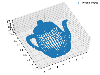
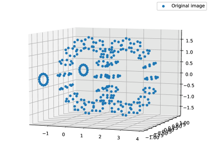
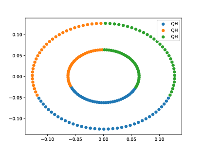
VI-E Point cloud image reconstruction
To illustrate that our CAFE-GCN algorithm in Algorithm 2 is able to perform dimensionality reduction well, we use the embedding vectors obtained from our algorithm to reconstruct several point cloud images that are transformed into a very high dimensional Euclidean space (by some measure-preserving transformations).
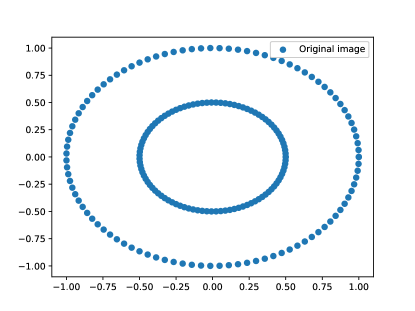
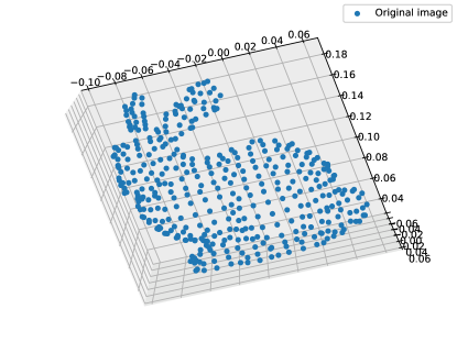
Specifically, we choose point cloud images, which are two concentric circles in 2D, Bunny in 3D [53], Teapot in 3D [54], and Junction in 3D [54] as our datasets (see Figure 3). Each point cloud image contains , , , and data points, respectively. Then we multiply the original data points by a (resp. ) orthogonal matrices for the 3D (resp. 2D) point cloud images and represent these transformed data points by an matrix. By doing so, each data point is transformed into an -vector. In this experiment, we set to be . We then subtract the column mean for each column of the matrix to obtain another matrix that has zero column sums. Then the matrix is a symmetric matrix with zero row sums and column sums. We then use our CAFE-GCN algorithm in Algorithm 2 with the input matrix to compute the -dimensional embedding vectors of the data points . Instead of removing the zero columns in in Step (2) of Algorithm 2, we keep all the columns to evaluate how similar the space spanned by all embedding vectors from Algorithm 2 and the space spanned by the eigenvectors are by calculating the square of the difference between the two vectors in (33) in Table IV. For the other inputs of Algorithm 2, we set the dimension of an embedding vector , and the inverse temperature .
| Point Cloud Image | in (33) | |||||
| 2D Two concentric circles | 0 | 0 | 0.5407 | 0.9492 | 0.9798 | 0.9800 |
| 3D Bunny | 0 | 0 | 0 | 0.8612 | 0.9208 | 0.9644 |
| 3D Teapot | 0 | 0 | 0 | 0.9392 | 0.9945 | 0.9994 |
| 3D Junction | 0 | 0 | 0 | 0.9827 | 0.4808 | 0.9043 |
From Table IV, we observe that there are three (resp. two) column vectors s that are very close to their projections s into the space spanned by the three (resp. two) dominant eigenvectors of the matrix in the 3D (resp. 2D) point cloud images. Note that the dominant eigenvectors of are the results of PCA for dimensionality reduction. This means the output of our CAFE-GCN in Algorithm 2 is able to compute the approximations of the dominant eigenvectors well and thus can also be used for dimensionality reduction. In fact, our numeral results (not shown in this paper) show that sphere-GCN is also able to perform the dimensionality reduction task.
To show the effectiveness of Algorithm 2, we select the column vectors from the output matrix that correspond to the closest projections into the space spanned by the dominant eigenvectors and plot the selected vectors. By doing so, the dimension of embedding vectors for 3D point cloud images (resp. 2D point cloud images) is three (resp. two). Figure 4 shows that the reconstructed point cloud images are almost the same as the original point cloud images. In order to visualize the clustering results, we apply a hard assignment on the soft assignment matrix , which is the output of the Algorithm 2 and obtain a partition matrix consisting of only and . The color of a data point represents the group it belongs to.
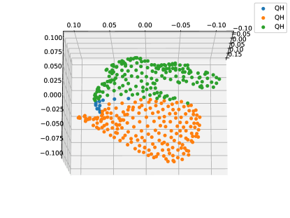
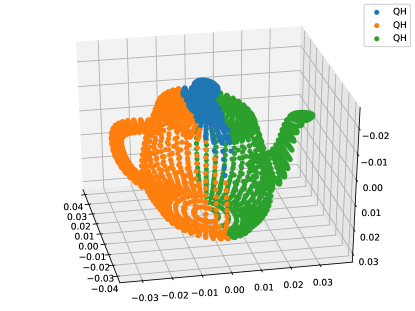
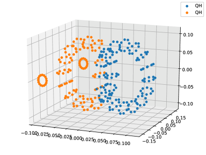
Looking deeper into the Junction dataset in Table IV and Figure 4, we find that Algorithm 2 is able to reconstruct the point cloud image and obtain good approximations of the top three dominant eigenvectors of . However, we only obtain two clusters from the partition matrix, which is different from the number of clusters in Step (4) of Algorithm 2. If we replace the soft assignment to the partition matrix in Step (3) of Algorithm 2, we can only get two dominant eigenvectors of . The reason is that all the none zero elements of are essential, no matter how small their probabilities are. We note that the hard assignment that outputs a partition matrix consisting of only and (colors of data points in Figure 4) discards important information of the number of linearly independent embedding vectors, especially for nodes or data points that are difficult to cluster (as those nodes exist small probabilities of being in another cluster). To explain this, suppose that the softmax function (soft assignment) outputs three linearly independent vectors and , where is very small after lots of iterations of softmax updates. Then using the hardmax function (hard assignment) forces to be . This leads to a result with only two linearly independent vectors and , and the dimension is reduced from to . As such, it is critical to keep the third linearly independent vector even though its coefficient is very small. For a community detection algorithm, what we care about is to which community a node is most likely assigned, and it is fine to use the hard assignment that sets elements with small probabilities to be zero. However, for the network embedding problem and the dimensionality reduction problem, it is crucial to keep most of the information by using the softmax function.
VII Conclusion
Based on the equivalence of the network embedding problem, the trace maximization problem, and the matrix factorization problem in a sampled graph, we proposed two explainable, scalable, and stable GCN algorithms for learning graph representations: (i) CAFE-GCN and (ii) sphere-GCN. We showed that both algorithms converge monotonically to a local optimum of the trace maximization problem in a sample graph, and thus yield good approximations of the dominant eigenvectors of the modularity matrix. The key difference between these two algorithms is the space of embedding vectors. CAFE-GCN maps each embedding vector into a probability vector through the softmax function, while sphere-GCN maps each embedding vector into a unit sphere. Both proposed GCNs are local methods as they only require local information from the node itself. As such, there are linear-time implementations for our proposed GCNs when the graph is sparse. In comparison with the proposed GCN methods, the power method is a global method that requires information from all the nodes for renormalization back to a unit -vector. As such, our GCN approaches are more scalable for large . In addition to solving the network embedding problem, both proposed GCNs are capable of performing dimensionality reduction.
Various experiments were conducted to evaluate our proposed GCNs. Our numerical results show that sphere-GCN outperforms almost all the baseline methods for node classification and link prediction tasks. Moreover, semi-supervised CAFE-GCN could be benefited from the labeled data and have tremendous improvements in various metrics. In particular, for the node classification task on the Cora dataset [32], CAFE-GCN (semi-supervised) achieves almost the same accuracy as the SplineCNN [52], which is the state-of-the-art method without using any side information.
Appendix A Proof of Theorem 6
We first show (28). Since is an orthonormal basis, the -vector can be represented as
| (37) |
where is the coordinate with respect to the orthonormal basis . Since , we have from (37) that
| (38) |
Using the fact that ’s are eigenvectors of yields
| (39) | |||||
From (25) and (38), it follows that
| (40) | |||||
In conjunction with (26), we then have
| (41) |
Now we show (29). Note that
| (42) | |||||
Analogous to the argument in (39) and (40), we have from the symmetry of that
| (43) | |||||
| (44) |
Moreover, using (43) in (42) yields
| (45) |
It is straightforward to verify that the function
is increasing in for . Using the lower bound for in (28) yields the lower bound for in (29).
Appendix B Proof of Theorem 7
First, we note that
| (46) |
where
As for all ,
which is a constant. Thus, it suffices to show that
is monotonically increasing after each iteration. Suppose that node is updated in Step (3) of Algorithm 4. Let after the update in Step (3) and after the re-normalization in Step (4). We will show that
| (47) |
Since
the vector is a convex combination of the two vectors and for , i.e., is in the segment between and . Thus, the angle between and is not larger than the angle between and for . This implies that
and thus the inequality in (47) holds.
References
- [1] W. L. Hamilton, R. Ying, and J. Leskovec, “Representation learning on graphs: Methods and applications,” arXiv preprint arXiv:1709.05584, 2017.
- [2] M. Belkin and P. Niyogi, “Laplacian eigenmaps and spectral techniques for embedding and clustering,” in Advances in neural information processing systems, 2002, pp. 585–591.
- [3] A. Ahmed, N. Shervashidze, S. Narayanamurthy, V. Josifovski, and A. J. Smola, “Distributed large-scale natural graph factorization,” in Proceedings of the 22nd international conference on World Wide Web, 2013, pp. 37–48.
- [4] S. Cao, W. Lu, and Q. Xu, “Grarep: Learning graph representations with global structural information,” in Proceedings of the 24th ACM international on conference on information and knowledge management, 2015, pp. 891–900.
- [5] M. Ou, P. Cui, J. Pei, Z. Zhang, and W. Zhu, “Asymmetric transitivity preserving graph embedding,” in Proceedings of the 22nd ACM SIGKDD international conference on Knowledge discovery and data mining, 2016, pp. 1105–1114.
- [6] B. Perozzi, R. Al-Rfou, and S. Skiena, “Deepwalk: Online learning of social representations,” in Proceedings of the 20th ACM SIGKDD international conference on Knowledge discovery and data mining, 2014, pp. 701–710.
- [7] A. Grover and J. Leskovec, “node2vec: Scalable feature learning for networks,” in Proceedings of the 22nd ACM SIGKDD international conference on Knowledge discovery and data mining, 2016, pp. 855–864.
- [8] T. N. Kipf and M. Welling, “Semi-supervised classification with graph convolutional networks,” arXiv preprint arXiv:1609.02907, 2016.
- [9] ——, “Variational graph auto-encoders,” arXiv preprint arXiv:1611.07308, 2016.
- [10] C.-S. Chang, C.-J. Chang, W.-T. Hsieh, D.-S. Lee, L.-H. Liou, and W. Liao, “Relative centrality and local community detection,” Network Science, vol. 3, no. 4, pp. 445–479, 2015.
- [11] C.-S. Chang, D.-S. Lee, L.-H. Liou, S.-M. Lu, and M.-H. Wu, “A probabilistic framework for structural analysis and community detection in directed networks,” IEEE/ACM Transactions on Networking, vol. 26, no. 1, pp. 31–46, 2017.
- [12] C.-S. Chang, C.-C. Huang, C.-T. Chang, D.-S. Lee, and P.-E. Lu, “Generalized modularity embedding: a general framework for network embedding,” arXiv preprint arXiv:1904.11027, 2019.
- [13] M. Rosvall and C. T. Bergstrom, “Maps of random walks on complex networks reveal community structure,” Proceedings of the National Academy of Sciences, vol. 105, no. 4, pp. 1118–1123, 2008.
- [14] R. Lambiotte, J.-C. Delvenne, and M. Barahona, “Random walks, markov processes and the multiscale modular organization of complex networks,” IEEE Transactions on Network Science and Engineering, vol. 1, no. 2, pp. 76–90, 2014.
- [15] M. Newman, Networks. Oxford university press, 2018.
- [16] S. Brin and L. Page, “The anatomy of a large-scale hypertextual web search engine,” Computer Networks and ISDN Systems, vol. 30, no. 1, pp. 107 – 117, 1998, proceedings of the Seventh International World Wide Web Conference. [Online]. Available: http://www.sciencedirect.com/science/article/pii/S016975529800110X
- [17] C.-T. Chang and C.-S. Chang, “A unified framework for sampling, clustering and embedding data points in semi-metric spaces,” arXiv preprint arXiv:1708.00316, 2017.
- [18] U. Von Luxburg, “A tutorial on spectral clustering,” Statistics and computing, vol. 17, no. 4, pp. 395–416, 2007.
- [19] W. Hamilton, Z. Ying, and J. Leskovec, “Inductive representation learning on large graphs,” in Advances in neural information processing systems, 2017, pp. 1024–1034.
- [20] Z. Ying, J. You, C. Morris, X. Ren, W. Hamilton, and J. Leskovec, “Hierarchical graph representation learning with differentiable pooling,” in Advances in neural information processing systems, 2018, pp. 4800–4810.
- [21] A. K. Bhowmick, K. Meneni, M. Danisch, J.-L. Guillaume, and B. Mitra, “Louvainne: Hierarchical louvain method for high quality and scalable network embedding,” in Proceedings of the 13th International Conference on Web Search and Data Mining, 2020, pp. 43–51.
- [22] B. Weisfeiler and A. A. Lehman, “A reduction of a graph to a canonical form and an algebra arising during this reduction,” Nauchno-Technicheskaya Informatsia, vol. 2, no. 9, pp. 12–16, 1968.
- [23] F. Scarselli, M. Gori, A. C. Tsoi, M. Hagenbuchner, and G. Monfardini, “The graph neural network model,” IEEE Transactions on Neural Networks, vol. 20, no. 1, pp. 61–80, 2008.
- [24] T. Wu, C.-S. Chang, and W. Liao, “Tracking network evolution and their applications in structural network analysis,” IEEE Transactions on Network Science and Engineering, vol. 6, no. 3, pp. 562–575, 2018.
- [25] G. Golub and C. Van Loan, Matrix Computations, ser. Johns Hopkins Studies in the Mathematical Sciences. Johns Hopkins University Press, 2013. [Online]. Available: https://books.google.com.tw/books?id=X5YfsuCWpxMC
- [26] D. K. Hammond, P. Vandergheynst, and R. Gribonval, “Wavelets on graphs via spectral graph theory,” Applied and Computational Harmonic Analysis, vol. 30, no. 2, pp. 129–150, 2011.
- [27] P. Sen, G. Namata, M. Bilgic, L. Getoor, B. Galligher, and T. Eliassi-Rad, “Collective classification in network data,” AI magazine, vol. 29, no. 3, pp. 93–93, 2008.
- [28] C. Yang, Z. Liu, D. Zhao, M. Sun, and E. Y. Chang, “Network representation learning with rich text information.” in IJCAI, vol. 2015, 2015, pp. 2111–2117.
- [29] J. Leskovec and J. J. Mcauley, “Learning to discover social circles in ego networks,” in Advances in neural information processing systems, 2012, pp. 539–547.
- [30] J. Tang, M. Qu, M. Wang, M. Zhang, J. Yan, and Q. Mei, “Line: Large-scale information network embedding,” in Proceedings of the 24th international conference on world wide web, 2015, pp. 1067–1077.
- [31] D. Wang, P. Cui, and W. Zhu, “Structural deep network embedding,” in Proceedings of the 22nd ACM SIGKDD international conference on Knowledge discovery and data mining, 2016, pp. 1225–1234.
- [32] P. with code, “Papers with code - cora benchmark (node classification).” [Online]. Available: https://paperswithcode.com/sota/node-classification-on-cora
- [33] M. E. Newman, “Fast algorithm for detecting community structure in networks,” Physical review E, vol. 69, no. 6, p. 066133, 2004.
- [34] C.-H. Chang, C.-S. Chang, C.-T. Chang, D.-S. Lee, and P.-E. Lu, “Exponentially twisted sampling for centrality analysis and community detection in attributed networks,” IEEE Transactions on Network Science and Engineering, vol. 6, no. 4, pp. 684–697, 2018.
- [35] S.-L. Huang, A. Makur, G. W. Wornell, and L. Zheng, “On universal features for high-dimensional learning and inference,” arXiv preprint arXiv:1911.09105, 2019.
- [36] E. Kokiopoulou, J. Chen, and Y. Saad, “Trace optimization and eigenproblems in dimension reduction methods,” Numerical Linear Algebra with Applications, vol. 18, no. 3, pp. 565–602, 2011.
- [37] C. M. Bishop, Pattern recognition and machine learning. springer, 2006.
- [38] P. W. Holland, K. B. Laskey, and S. Leinhardt, “Stochastic blockmodels: First steps,” Social networks, vol. 5, no. 2, pp. 109–137, 1983.
- [39] A.-L. Barabási and R. Albert, “Emergence of scaling in random networks,” science, vol. 286, no. 5439, pp. 509–512, 1999.
- [40] W. W. Zachary, “An information flow model for conflict and fission in small groups,” Journal of anthropological research, vol. 33, no. 4, pp. 452–473, 1977.
- [41] J. Leskovec, J. Kleinberg, and C. Faloutsos, “Graph evolution: Densification and shrinking diameters,” ACM transactions on Knowledge Discovery from Data (TKDD), vol. 1, no. 1, pp. 2–es, 2007.
- [42] C.-C. J. Kuo, “Understanding convolutional neural networks with a mathematical model,” Journal of Visual Communication and Image Representation, vol. 41, pp. 406–413, 2016.
- [43] ——, “The cnn as a guided multilayer recos transform [lecture notes],” IEEE signal processing magazine, vol. 34, no. 3, pp. 81–89, 2017.
- [44] F. Rosenblatt, “The perceptron: a probabilistic model for information storage and organization in the brain.” Psychological review, vol. 65, no. 6, p. 386, 1958.
- [45] V. D. Blondel, J.-L. Guillaume, R. Lambiotte, and E. Lefebvre, “Fast unfolding of communities in large networks,” Journal of statistical mechanics: theory and experiment, vol. 2008, no. 10, p. P10008, 2008.
- [46] T. Mikolov, I. Sutskever, K. Chen, G. S. Corrado, and J. Dean, “Distributed representations of words and phrases and their compositionality,” in Advances in neural information processing systems, 2013, pp. 3111–3119.
- [47] M. Khosla, A. Anand, and V. Setty, “A comprehensive comparison of unsupervised network representation learning methods,” arXiv preprint arXiv:1903.07902, 2019.
- [48] L. Katz, “A new status index derived from sociometric analysis,” Psychometrika, vol. 18, no. 1, pp. 39–43, 1953.
- [49] H. H. Song, T. W. Cho, V. Dave, Y. Zhang, and L. Qiu, “Scalable proximity estimation and link prediction in online social networks,” in Proceedings of the 9th ACM SIGCOMM conference on Internet measurement, 2009, pp. 322–335.
- [50] C. F. Van Loan, “Generalizing the singular value decomposition,” SIAM Journal on numerical Analysis, vol. 13, no. 1, pp. 76–83, 1976.
- [51] T. Chen and C. Guestrin, “XGBoost: A scalable tree boosting system,” in Proceedings of the 22nd ACM SIGKDD International Conference on Knowledge Discovery and Data Mining, ser. KDD ’16. New York, NY, USA: ACM, 2016, pp. 785–794. [Online]. Available: http://doi.acm.org/10.1145/2939672.2939785
- [52] M. Fey, J. Eric Lenssen, F. Weichert, and H. Müller, “Splinecnn: Fast geometric deep learning with continuous b-spline kernels,” in Proceedings of the IEEE Conference on Computer Vision and Pattern Recognition, 2018, pp. 869–877.
- [53] R. B. Rusu and S. Cousins, “3D is here: Point Cloud Library (PCL),” in 2011 IEEE International Conference on Robotics and Automation (ICRA). Shanghai, China: IEEE, May 9-13 2011.
- [54] N. Joubert and J. Andrews, “Cs148 assignment 3: Raytracing,” Jul 2010. [Online]. Available: http://graphics.stanford.edu/courses/cs148-10-summer/as3/as3.html
![[Uncaptioned image]](/html/2009.10367/assets/pelu.jpg) |
Ping-En Lu (GS’17) received his B.S. degree in communication engineering from the Yuan Ze University, Taoyuan, Taiwan (R.O.C.), in 2015. He is currently pursuing the Ph.D. degree in the Institute of Communications Engineering, National Tsing Hua University, Hsinchu, Taiwan (R.O.C.). He won the ACM Multimedia 2017 Social Media Prediction (SMP) Challenge with his team in 2017. His research interest is in network science, efficient clustering algorithms, network embedding, and deep learning algorithms. He is an IEEE Graduate Student Member. |
![[Uncaptioned image]](/html/2009.10367/assets/x10.png) |
Cheng-Shang Chang (S’85-M’86-M’89-SM’93-F’04) received the B.S. degree from National Taiwan University, Taipei, Taiwan, in 1983, and the M.S. and Ph.D. degrees from Columbia University, New York, NY, USA, in 1986 and 1989, respectively, all in electrical engineering. From 1989 to 1993, he was employed as a Research Staff Member with the IBM Thomas J. Watson Research Center, Yorktown Heights, NY, USA. Since 1993, he has been with the Department of Electrical Engineering, National Tsing Hua University, Taiwan, where he is a Tsing Hua Distinguished Chair Professor. He is the author of the book Performance Guarantees in Communication Networks (Springer, 2000) and the coauthor of the book Principles, Architectures and Mathematical Theory of High Performance Packet Switches (Ministry of Education, R.O.C., 2006). His current research interests are concerned with network science, big data analytics, mathematical modeling of the Internet, and high-speed switching. Dr. Chang served as an Editor for Operations Research from 1992 to 1999, an Editor for the IEEE/ACM TRANSACTIONS ON NETWORKING from 2007 to 2009, and an Editor for the IEEE TRANSACTIONS ON NETWORK SCIENCE AND ENGINEERING from 2014 to 2017. He is currently serving as an Editor-at-Large for the IEEE/ACM TRANSACTIONS ON NETWORKING. He is a member of IFIP Working Group 7.3. He received an IBM Outstanding Innovation Award in 1992, an IBM Faculty Partnership Award in 2001, and Outstanding Research Awards from the National Science Council, Taiwan, in 1998, 2000, and 2002, respectively. He also received Outstanding Teaching Awards from both the College of EECS and the university itself in 2003. He was appointed as the first Y. Z. Hsu Scientific Chair Professor in 2002. He received the Merit NSC Research Fellow Award from the National Science Council, R.O.C. in 2011. He also received the Academic Award in 2011 and the National Chair Professorship in 2017 from the Ministry of Education, R.O.C. He is the recipient of the 2017 IEEE INFOCOM Achievement Award. |