Twin Null-Point-Associated Major Eruptive Three-Ribbon Flares with Unusual Microwave Spectra

1 Introduction

S-introduction

Solar eruptions, flares, and similar weaker events draw energy from coronal magnetic fields. Such events span over a vast range of energy and time scales and spatial extent and manifest in various associated phenomena. The way in which an eruption (flare) develops, its manifestations and particularities depend on the magnetic configuration that hosts the event and magnetic-field transformations that occur in its course. Magnetic reconnection is considered as the key process that governs solar eruptions and flares.

Several properties of a two-ribbon flare and its development have mainly been explained by the two-dimensional (2D) standard model (CSHKP: Carmichael, 1964; Sturrock, 1966; Hirayama, 1974; Kopp and Pneuman, 1976). Reconnection in this model occurs in an X-point of a vertical current sheet, which is formed due to the rise of a prominence driven by a current instability (Hirayama, 1974). The flare was implicitly presumed to be caused by the prominence eruption, whose development was not considered. In modern models of two-ribbon flares, the prominence is replaced by a magnetic flux-rope. When the standard flare model is generalized to a 3D situation, new particularities appear in magnetic reconnection and the shapes and location of paired flare ribbons that are absent in 2D models (see, e.g., Aulanier, Janvier, and Schmieder, 2012; Janvier et al., 2013 and references therein).

Two conditions are necessary for the development of a large-scale current instability that leads to the flux-rope expansion. These are i) formation in the corona of a flux rope, where the twist [$N$] of magnetic-field lines certainly exceeds unity ($N>1$), and ii) its rise to a height, starting from which the expansion becomes continuous. The second condition is met, if the component of the external magnetic field transversal to the flux-rope axis falls off with height fast enough.

The way widely used for the formation of a magnetic flux-rope and initiation of a two-ribbon flare invokes as boundary conditions different types of photospheric plasma motions such as shear, converging, or rotational motions (e.g. Inhester, Birn, and Hesse, 1992; Longcope and Beveridge, 2007). A shorter way is also possible. In the dual-filament model (Uralov et al., 2002; Grechnev et al., 2006; see also Hansen, Tripathi, and Bellan, 2004), low-corona reconnection between two or more filament sections and between their threads (barbs) increases the length and height of the combined filament. This increases its dipole momentum and the total twist up to $N>1$, launching the standard-model reconnection.

Relatively recently, 3D coronal configurations with a null-point topology (NPT) have been identified above photospheric magnetic islands surrounded by opposite-polarity environment (e.g. Filippov, 1999; Filippov, Golub, and Koutchmy, 2009; Masson et al., 2009; Meshalkina et al., 2009; Pariat, Antiochos, and DeVore, 2009, 2010; Reid et al., 2012; Wang and Liu, 2012). Such configurations are ubiquitous, being responsible for a variety of phenomena from tiny polar X-ray jets up to major flares. A flare that occurs in an NPT-configuration produces a circular ribbon with a brightening in the center. An implicated remote compact site is sometimes detectable.

According to Filippov, Golub, and Koutchmy (2009) and Meshalkina et al. (2009), a reconnection event in an NPT-configuration is generally initiated and governed by the eruption of a small flux-rope-like structure that occurs inside an inverted-funnel-like separatrix surface. Reconnection behind the erupting structure occurs in the same way as in a usual two-ribbon flare. When the eruption passes through the null-point region, its magnetic structure becomes partly or entirely destroyed. A jet is ejected in the latter case (see also Sterling et al., 2016 who came to similar conclusions). This sequence of events is supported by a half-minute delay of the hard X-ray burst relative to the acceleration of the erupting structure measured by Grechnev et al. (2011a) in the event that Meshalkina et al. (2009) considered, where a bright ring-like structure and broad jet were observed in the extreme ultraviolet. Conversely, the numerical magnetohydrodynamic (MHD) simulations of Pariat, Antiochos, and DeVore (2009, 2010) and Masson et al. (2009, 2017) do not require small flux-rope eruptions as significant components of their NPT-associated models of flares and jets (see also a review by Raouafi et al., 2016).

Larger-scale phenomena probably caused by reconnection between magnetic structures of erupting filaments and static coronal environment have also been sometimes observed. They are manifested in bifurcation of an erupting structure and dispersal of the erupted material over a large surface far from the eruption region (Slemzin et al., 2004; Grechnev et al., 2005, 2014; Uralov et al., 2014). The dispersed low-temperature material released by reconnection from the filament body can screen large areas on the Sun and cause an extensive darkening in 304 Å and depression of the total microwave flux (Grechnev et al., 2008, 2011b, 2013b). Reconnection in such events is forced by the expansion of an erupting structure that encounters a topological obstacle in its path in the corona. A similar conclusion was drawn by van Driel-Gesztelyi et al. (2014) for the spectacular SOL2011-06-07 event.

While MHD simulations demonstrate the possibility of reconnection in an NPT-configuration without any eruption, observations indicate that such phenomena are caused by interactions of erupting structures with static coronal magnetic fields. In this respect, flares in NPT-configurations do not seem to be considerably different from usual eruptive two-ribbon flares, where flare processes are caused by eruptions that basically corresponds to the scenario of Hirayama (1974). This relation is supported by the correspondence between the kinematics of an erupting structure and flare emissions, which were delayed by up to two minutes that was found in studies of several eruptive events of different types and importance (Grechnev et al., 2011a, 2013a, 2015, 2016, 2019). On the other hand, in the absence of eruptions, coronal null points are steady and do not reveal themselves in any way (e.g. Filippov, 1999; Grechnev et al., 2014) that does not favor the scenario, in which an event starts from the null-point reconnection itself.

The morphology was still more outstanding in the events presented by Wang et al. (2014). The authors addressed a pair of successive flares (M1.9 and C9.2) that occurred on 6 July 2012 within half an hour and both exhibited unusual three-ribbon configuration. The flares were accompanied by surges and jets. The authors conjectured that the events were caused by reconnection along the coronal null line in the fan–spine magnetic topology. Bamba et al. (2017) presented a three-ribbon flare that occurred on 25 October 2014.

We consider a pair of three-ribbon flares that also occurred within half an hour in the same active region on 23 July 2016. The flares (M7.6 and M5.5) were stronger than those addressed by Wang et al. (2014), both of them were eruptive and produced conspicuous emissions in microwaves, hard X-rays, and $\gamma$-rays. The clear presence of filament eruptions in both events removes the question of their possible involvement. The large size of the flares favors the analysis of various manifestations that were barely detectable in weaker events. Taking advantage of these unprecedented observations, we address the properties of the two eruptive flares, reveal the magnetic configuration where they occurred, and pursue understanding their common scenario.

Section S-overview briefly overviews the twin events and highlights their particularities. Section S-configuration_scenario addresses the coronal configuration, where the events occurred, and infers their scenario. Section S-acc_electrons addresses manifestations of accelerated electrons in microwave and hard X-ray images and considers the spectra in the two spectral domains. Section S-conclusion summarizes the results. The AIA335.mpg, pot˙Br˙mod˙B.mpg, and nlff˙Br˙mod˙B.mpg movies in the Electronic Supplementary Material illustrate the twin events and particularities of the coronal magnetic configuration.

2 Overview of the Twin Events

S-overview

2.1 Microwave and Hard X-Ray Non-Imaging Data

S-microwaves_HXR

The Siberian Radioheliograph (SRH: Lesovoi et al., 2014, 2017) commenced test-mode observations early in 2016. In summer 2016, the SRH started to observe the Sun routinely at five frequencies of 4.5, 5.2, 6.0, 6.8, and 7.5 GHz along with the ongoing adjustment of its systems. The temporal interval to scan the five frequencies was 8.4 seconds at that time. The longest SRH baseline of 107.4 m determines its spatial resolution of order $100^{\prime\prime}$ (depending inversely on frequency) that allows locating a microwave source on the Sun but is insufficient to reveal its shape and structure. Real-time beacon SRH data at a set of the operating frequencies with an update every minute are accessible online at the SRH Web site badary.iszf.irk.ru/.

On 23 July 2016, the SRH recorded strong microwave bursts associated with two major flares that occurred within half an hour at N05 W73 in active region, whose parts were numbered 12565 and 12567. The GOES importance was M7.6 for the first flare and M5.5 for the second flare. The Badary Broadband Microwave Spectropolarimeters (BBMS: Zhdanov and Zandanov, 2011, 2015; Kashapova et al., 2013) that are installed near the SRH measured the total flux up to 400 sfu in the first flare and up to 800 sfu in the second flare.

Figure F-time_prof shows the temporal profiles recorded during the two flares in microwaves and hard X-rays (HXR). Figure F-time_profa presents the so-called correlation plots produced by the SRH that are computed without synthesizing the images as the sum of cross-correlations between all antenna pairs (Lesovoi and Kobets, 2017). The correlation plots represent a proxy of total-flux variations, responding to the changes in both the brightness and structure of microwave sources. To get indications at total-flux spectra of the sources that were unresolved in these observations, each $i$-th correlation plot obtained at a frequency $\nu_{i}$ was multiplied by $\left(\nu_{i}/\overline{\nu}\right)^{2}$, where $\overline{\nu}$ is the average frequency of the SRH observing range.

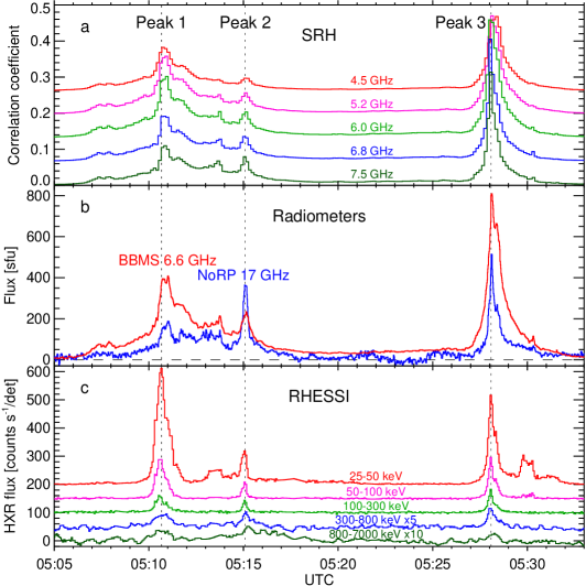
Figure 1.: Temporal profiles of the two flare bursts. (a) Correlation plots recorded by the SRH. (b) Microwave bursts recorded by total-flux radiometers at 6.6 GHz (BBMS) and 17 GHz (NoRP). (c) Hard X-ray and $\gamma$-ray bursts observed by RHESSI. Two highest-energy count rates are smoothed and magnified by factors of 5 (300 – 800 keV) and 10 (800 – 7000 keV). The background levels on panels a and c are shifted to show the bursts better. The vertical dotted lines mark three main peaks that are detectable in all ranges.F-time˙prof

Three main peaks numbered 1 – 3 are distinct. Comparison of the peaks at different SRH frequencies indicates that the turnover frequencies (peak frequencies of the spectra) for peaks 1 and 3 were within the SRH range or nearby and higher for peak 2. These indications are confirmed in Figure F-time_profb that presents total-flux variations recorded by the BBMS at 6.6 GHz and by the Nobeyama Radio Polarimeters (NoRP: Torii et al., 1979; Nakajima et al., 1985) at 17 GHz. The peaks had different spectra indeed: while peaks 1 and 3 were stronger at 6.6 GHz, peak 2 was stronger at 17 GHz.

Figure F-time_profc presents HXR and $\gamma$-ray bursts recorded by the Reuven Ramaty High-Energy Solar Spectroscopic Imager (RHESSI: Lin et al., 2002) in five energy bands. To reduce the variable background, whose importance increases with increasing energy, its variations in the preceding and following orbits were fitted for each energy band and subtracted. To enhance the signal-to-noise ratio in the two highest-energy bands plotted, the count rates were smoothed with a boxcar average over three neighbors for the 300 – 800 keV band and over five neighbors for the 800 – 7000 keV band. They are magnified in Figure F-time_profc. The three main peaks became detectable at energies exceeding 800 keV.

It is possible to judge qualitatively about the photon HXR spectra by comparing visually the heights of the peaks in a high-energy band (e.g. 300 – 800 keV) and in the 25 – 50 keV band. Peak 1 had the softest photon spectrum, peak 2 had the hardest spectrum, and the spectrum of peak 3 was in between of them. The same relation is expected for high-frequency parts of the microwave spectra of the three peaks (Dulk and Marsh, 1982; White et al., 2011).

Figure F-mw_spectra present total-flux microwave spectra of integrated over eight seconds around each peak. We used one-second NoRP data, one-second data obtained at the Learmonth station of the US Air Force Radio Solar Telescope Network (RSTN: Guidice, 1979; Guidice et al., 1981), and BBMS data with a temporal sampling of 1.6 seconds. The whole data set had problems. The BBMS consists of two instruments, each of which employs its own spectrum analyzer. The 4 – 8 GHz spectropolarimeter operated in the high-sensitivity mode so that its data were saturated. A few channels of the 2 – 24 GHz spectropolarimeter were out of operation. The triangles in Figure F-mw_spectra in the 2.34 – 10.1 GHz range represent the data from the BBMS channels that appear to be reliable.

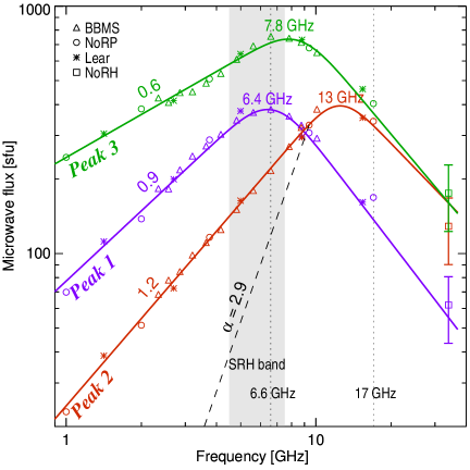
Figure 2.: Microwave spectra of the three peaks denoted in Figure F-time_prof composed from measurements at different total-flux radiometers and NoRH (symbols). The thick color curves represent their simplest fit, from which the peak frequencies indicated near the spectral peaks were estimated. The slopes of the high-frequency branches have considerable uncertainties. The slanted dashed line demonstrates the theoretical slope $\alpha=2.9$ expected at low frequencies for a single gyrosynchrotron source if it were responsible for peak 2. The shading denotes the SRH observing frequency range. The vertical dotted lines denote the frequencies of 6.6 and 17 GHz, at which the time profiles presented in Figure F-time_profb were measured.F-mw˙spectra

To find the slope of the descending part of the microwave spectrum, high-frequency measurements are important. However, the total-flux variations shown by NoRP at 35 GHz are strongly dissimilar to the temporal profiles recorded at lower frequencies. This indicates improper operation of the 35 GHz instrument. We had to use instead the images produced by the Nobeyama Radioheliograph (NoRH: Nakajima et al., 1994) at 34 GHz. NoRH suffered in this period from hardware problems. We synthesized NoRH images at 34 GHz around each of the three peaks with intervals and integration times of one second and five seconds. The images in each set were coaligned with each other. To calibrate the images in brightness temperatures, the regions of the solar disk and the sky were analyzed separately, and the most-frequent pixel values were referred to $10^{4}$ K and zero, respectively (Kochanov et al., 2013). The one-second image set was subjected to the median smoothing along each pixel with widths of three and five. Then, the total flux was computed over the flaring region from all image sets. Comparison of the results with each other indicates the calibration stability of the reduced-quality NoRH 34 GHz images of about $\pm 30\%$. The squares in Figure F-mw_spectra represent probable fluxes at 34 GHz with the $\pm 30\%$ uncertainties shown by the bars.

The ascending and descending branches of the microwave spectra were analyzed separately using the linear fit in the log–log scale. Because of the insufficient measurement accuracy at 34 GHz, the slopes of the high-frequency branches have increased uncertainties, especially for peak 2. The two branches were connected with the antiderivative (indefinite integral) of the error function. The peak frequencies estimated from the fitting curves are indicated at the curves along with low-frequency slopes [$\alpha$] found from the linear fit. The positions of the estimated peak frequencies relative to the SRH frequency range (the shading) are consistent with the assessments that were made from the correlation plots in Figure F-time_profa, while the ongoing adjustment of the SRH hardware systems disfavored accurate calculations of the flux spectrum from the images at that time.

The low-frequency branches of the spectra are flattened with respect to the theoretical slope $\alpha=2.9$ expected for a simple single gyrosynchrotron source. This slope is shown by the dashed line for peak 2. A possible cause of the low-frequency spectral flattening may be asymmetry of the flaring magnetic configuration; the magnetic-flux balance requires a larger area of a weaker-field side than of the conjugate region that elevates the low-frequency spectral part and shifts the peak frequency to the left (Grechnev et al., 2017). The change from peak 2 to peak 3 seems to be especially challenging, because no change in most of the parameters that govern gyrosynchrotron emission displaces the top of its spectrum up and left (Stähli, Gary, and Hurford, 1989). These circumstances indicate that the flare configuration was asymmetric and relatively complex.

2.2 Two Successive Eruptions

S-two_eruptions

The paired events comprised two sequential eruptions that were observed in all extreme-ultraviolet (EUV) channels of the Atmospheric Imaging Assembly (AIA) on board the Solar Dynamics Observatory (SDO: Lemen et al., 2012). The two eruptions are demonstrated by the 2016-07-23˙AIA335.mpg Electronic Supplementary Material. The movie was composed from the images obtained in the low-sensitivity 335 Å AIA channel, which did not suffer from saturation.

Figure F-two_events presents a few episodes of the two eruptive events. Event 1 started from the eruption of the first filament, Fil1, in Figure F-two_eventsa that corresponds to the time of peak 1 in Figure F-time_prof. The filament brightened up, inflated (Figure F-two_eventsb), and expanded further. The ragged appearance of the erupting filament in Figure F-two_eventsc indicates that its structure became partly damaged. Arcade Arc1 in Figure F-two_eventsd appeared in the first event, whose GOES importance reached a level of M7.6. The yellow contour in Figure F-two_eventsb presents the unresolved microwave source observed by the SRH at 6.0 GHz at a half-height level that is close to the SRH beam.

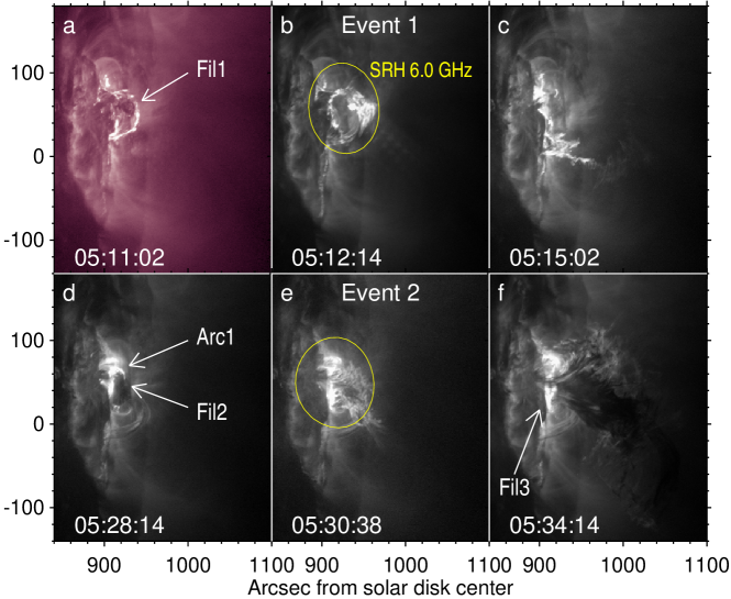
Figure 3.: Two eruptive events observed within half an hour by SDO/AIA in 211 Å. The yellow contours on panels b and e represent the SRH 6.0 GHz images at half-height levels. The arrows indicate eruptive filaments Fil1 and Fil2. Arcade Arc1 formed in the first event is visible. Filament Fil3 did not erupt and partly blocked in EUV the second, southern arcade.F-two˙events

The second event associated with the eruption of another filament, Fil2 (Figures F-two_eventsd – F-two_eventsf), was mainly similar to the first event. Figure F-two_eventsd corresponds to the time of peak 3 in Figure F-time_prof. The structure of the second filament was also damaged; dark filament material dispersed and partly returned back to the solar surface (Figure F-two_eventsf). The third filament, Fil3, denoted in Figure F-two_eventsf exhibited motions, but did not erupt. This filament partly hid the southern flare arcade in EUV. The GOES importance of the second event was M5.5. The yellow contour in Figure F-two_eventse presents the 6.0 GHz SRH image (similar to Figure F-two_eventsb).

The two-fold character of the whole event manifested in associated phenomena. Each of the two eruptions produced an EUV wave (Chandra et al., 2018). The online CME catalog (cdaw.gsfc.nasa.gov/CME˙list/: Yashiro et al., 2004) presents an associated CME, whose faster northern part was followed by a slower southern part that was launched apparently later.

2.3 Three-Ribbon Flare Configuration

S-three_ribbon

A particularity of the two corresponding flares was their three-ribbon configuration. High brightness of the flare ribbons caused strong overexposure distortions in the 1600 Å SDO/AIA channel. The 1700 Å AIA images were also saturated, but their quality was better. Figure F-three_ribbons presents the flare ribbons observed by AIA in 1700 Å in the two flares near the three main peaks. The contours overlaid on the images represent the polarities of the radial magnetic component that was computed from vector magnetograms produced on 23 July by the Helioseismic and Magnetic Imager (HMI: Scherrer et al., 2012) on board SDO.

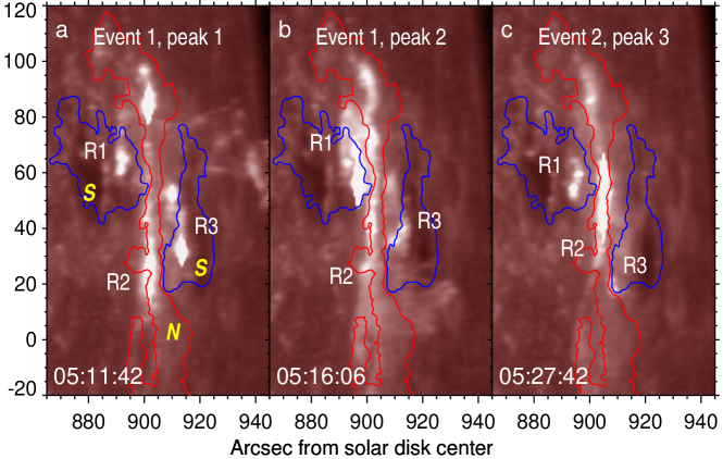
Figure 4.: Three-ribbon configurations observed by SDO/AIA in 1700 Å in the two flares near the three main peaks. The blue contours outline the S-polarity radial magnetic component, and the red contour outlines the N-polarity region. The contour levels are $[-240,+120]$ G.F-three˙ribbons

Each of the three panels in Figure F-three_ribbons shows a long N-polarity middle ribbon R2 and two considerably shorter ribbons R1 and R3 in S-polarity regions on both sides of the middle ribbon. The three-ribbon configuration corresponds to the S – N – S structure of ribbons R1 – R2 – R3. The magnetic fields within the contours were stronger in the S-polarity regions than in the N-polarity region by a factor of about 2.3 on the average. The shorter lengths of the S-polarity ribbons are determined by the magnetic-flux balance at the conjugate regions. This circumstance confirms the indications suggested by the shapes of the microwave spectra that were outlined in Section S-microwaves_HXR.

3 Coronal Magnetic Configuration and Scenario of the Events

S-configuration_scenario

3.1 Magnetic Configuration

S-configuration

The 23 July twin events were located not far from the limb, where considerable projection shrinkage complicates the understanding of the magnetic configuration. We firstly consider observations of the active region, which hosted the events, that were made a few days before. The active region observed by SDO/HMI on 20 July is shown in Figures F-mag_configa (intensitygram) and F-mag_configb (line-of-sight magnetogram). Two S-polarity sunspots Ss1 and Ss2 were separated by an extended N-polarity plage region PR. No conspicuous flare manifestations were visible near the eastern N-polarity sunspot Ss3. The magnetic field in the plage region strengthened from 20 to 23 July.

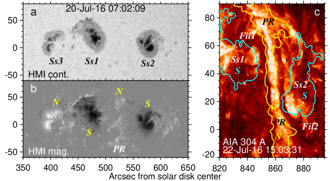
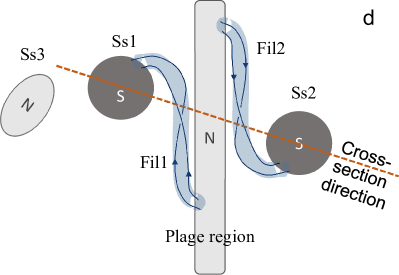
Figure 5.: Pre-flare configuration. Intensitygram (a) and line-of-sight magnetogram (b) of the active region observed by SDO/HMI on 20 July, three days before the events. The yellow labels N and S denote magnetic polarities of sunspots Ss1, Ss2, and Ss3, and plage region PR. (c) SDO/AIA 304 Å image observed on 22 July presents two filaments Fil1 and Fil2 located between the S-polarity sunspots Ss1 and Ss2 and N-polarity plage region PR. (d) A scheme of the magnetic configuration inferred from observations. The slanted brown-dashed line denotes the direction of the cross-section that is presented in Figure F-scenario.F-mag˙config

Figure F-mag_configc presents a 304 Å AIA image observed 14 hours before the events along with contours of the radial magnetic component computed from a simultaneous HMI vector magnetogram. Two filaments are visible in 304 Å. Filament Fil1 was rooted by the northern end in the S-polarity environment of sunspot Ss1 and mostly located above the neutral line between the Ss1 environment and the plage region PR. Filament Fil2 was rooted by the southern end in the S-polarity environment of sunspot Ss2 and mostly located above the neutral line between the Ss2 environment and PR. The opposite ends of both filaments must be rooted in an N-polarity region, i.e. in the plage region PR. These circumstances are shown in the scheme of the magnetic configuration presented in Figure F-mag_configd.

The analysis of the observations and magnetic fields reconstructed in the corona allowed us to infer the coronal configuration, where the two events occurred, and their scenario that is considered in the next section. Figure F-extrap presents the coronal configuration reconstructed from an SDO/HMI magnetogram in the potential-field approximation. Two sets of low loops, which are rooted in the extended plage region, go into opposite directions that indicates the presence of a separatrix surface between them. One set of loops connects the plage region with sunspot Ss1 and the other connects the plage region with sunspot Ss2. The magnetic flux coming into the S-polarity sunspots is not compensated by the flux outgoing from the N-polarity plage region. An excessive portion of the S-polarity flux is outgoing from the remote N-polarity sunspot Ss3 and its environment. The magnetic configuration suggests the possible presence of a coronal null point or even a portion of a null line where the magnetic-field magnitude $|\textbf{{B}}|$ is zero.

To verify these conjectures, we investigate the spatial distribution of the coronal magnetic field computed above the active region using the potential approximation (e.g. Uralov, Rudenko, and Rudenko, 2006; Uralov et al., 2008; Grechnev et al., 2014) and non-linear force-free reconstruction that is based on the optimization method by Wheatland, Sturrock, and Roumeliotis (2000) as implemented by Rudenko and Myshyakov (2009). The first stage of our approach is to analyze the behavior of the null line of the radial magnetic component $B_{r}$ at different heights. The presence of a real null point (which is not an issue of noise or small-scale uncertainties) is visually indicated by the bifurcation of the $B_{r}=0$ line that occurs as the height changes. The bifurcation appears as the convergence of the $B_{r}=0$ lines followed by their visual “reconnection” and subsequent divergence in the orthogonal direction of the $B_{r}=0$ lines that are newly formed. If the bifurcation occurs in both force-free and potential approximations, then the null point (or line) is an element of a sufficiently large-scale magnetic topology. To locate the null point or line accurately, the behavior of the magnetic-field magnitude $|\textbf{{B}}|$ in the vicinity of the bifurcation region is analyzed.

The pot˙Br˙mod˙B.mpg and nlff˙Br˙mod˙B.mpg movies in the Electronic Supplementary Material demonstrate the behaviors of the $B_{r}=0$ line (red) and $|\textbf{{B}}|$ (gray scale and green contour) in the potential and force-free approximations, respectively. We are interested in the region of the null point that is denoted with a circle in the potential approximation and with two slanted crosses in the force-free approximation. In the latter case, the only null point exists (lower cross) instead of a null line. From the null point, a line toward the second cross extends with $B_{r}$ nearly zero, but with a weak quasi-transversal magnetic component. The heights of the null points are noticeably different in the potential (between 16 and 17 Mm) and force-free (between 23 and 24 Mm) approximations.

The configuration presented in Figure F-extrap is similar to the quasi-circular configuration with a null point that was considered previously by Filippov, Golub, and Koutchmy (2009), Masson et al. (2009), and Meshalkina et al. (2009). Wang et al. (2014) analyzed a configuration where paired M1.9 and C9.2 three-ribbon flares occurred that were less powerful than our events and had not caused any noticeable CME. Unlike our approach, Wang et al. (2014) envisioned the presence of the null line by inference.

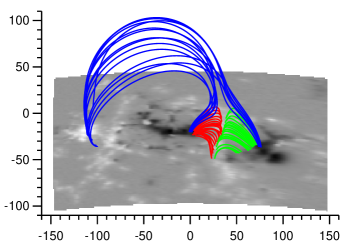
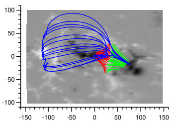
                                  a                                         b

Figure 6.: Reconstructed coronal magnetic configuration: (a) side view, (b) top view. The gray-scale background shows the magnetogram at the photospheric level. The red and green field lines represent two arcades. The blue lines represent the field lines of the excessive magnetic flux that is rooted in the remote eastern N-polarity sunspot and its environment. The axes show arc seconds from the center of the region considered.F-extrap

3.2 Scenario

S-scenario

Our analysis of observations in different spectral ranges has led to a scenario of the twin events. For simplicity we consider the 2D geometry that is justified to some extent by the presence near the magnetic null point of an extended (about 15 Mm) linear region where magnetic field is weak. The scenario is schematically shown in Figure F-scenario that presents magnetic domains separated from each other by sepatratrices (broken lines). Each of the inner domains contains a filament (blue disk). In Figure F-scenarioa, filament 1 in the inner-left domain starts to lift-off gradually during the initiation phase, while filament 2 in the inner-right domain remains static so far.

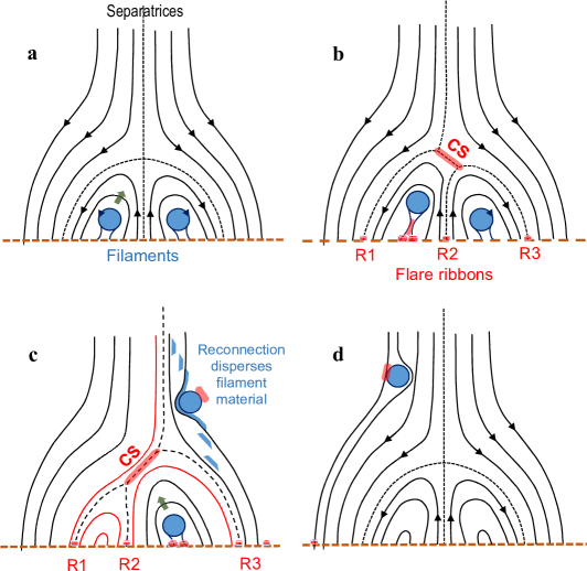
Figure 7.: Two-dimensional scheme of the scenario of the two eruptive events: Side view at the cross-section in the direction indicated in Figure F-mag_configd by the slanted brown-dashed line. The solid lines represent magnetic-field lines, the dashed lines represent separatrices, the blue disks represent cross-sections of eruptive filaments, and the thick pink bars represent current sheets. (a) The first filament starts to lift-off. (b) The rise of the erupting filament results in the formation of the current sheet (CS). Three flare ribbons R1, R2, and R3 appear. (c) After the passage of the null, the first erupting filament (flux-rope progenitor) intensively reconnects in the outer-right magnetic domain. The current sheet changes orientation, facilitating the second eruption. (d) The second filament passes the null and also undergoes reconnection. After that, relaxation of the configuration to the steady state begins.F-scenario

Reconnection inside the inner-left domain in Figure F-scenariob starts transforming filament 1 into a flux rope. A current instability of this flux-rope progenitor (henceforth flux rope) triggers its sharp eruption with a motion directed to the null point. The current sheet (pink bar) forms from the null point and transfers the magnetic flux into adjacent domains, displacing the separatrices. Reconnection beneath the erupting structure reinforces flare energy release (not shown). Accelerated particles stream down along the field lines, precipitate in dense layers, and produce HXR emission. Three main flare ribbons R1, R2, and R3 appear.

After the passage of the null in Figure F-scenarioc, the first erupting flux rope enters the outer-right domain where its azimuthal magnetic component becomes antiparallel to the coronal environment. The flux rope intensively reconnects with environment and transfers kinetic energy and magnetic helicity to the reconnected magnetoplasma. Portions of the filament material are released (blue) and scatter along the field lines. New field lines (red) appear in adjacent domains. The current sheet changes orientation that favors the recovery of their positions. This trend facilitates the second eruption.

Then, filament 2 erupts and repeats the history of filament 1. After the passage of the null in Figure F-scenariod, the second flux rope also undergoes reconnection that results in the dispersal of its material. Eventually, the configuration relaxes and returns to the original state.

The features of this scenario are determined by properties of the coronal configuration. Quasi-circular funnel-like configurations with magnetic null points exist ubiquitously above small magnetic islands within the opposite-polarity environment. Nevertheless, three-ribbon flares are very rare. The particularity of the configuration in our case was the presence of a coronal magnetic quasi-null line with almost zero radial component and small transversal components that made the geometry quasi-two-dimensional. In the scenario described in this section, the first eruption causes the second that was also the case in the events addressed by Wang et al. (2014).

4 Manifestations of Accelerated Electrons

S-acc_electrons

4.1 Hard X-Ray and Microwave Images

S-HXR_mw_images

As shown in Section S-microwaves_HXR, the twin events emitted conspicuous microwaves, hard X-rays, and $\gamma$-rays that are produced by accelerated electrons. We compare their manifestations with EUV images using microwave NoRH (Nakajima et al., 1994) and HXR RHESSI (Lin et al., 2002) data. The NoRH enhanced-resolution images at 17 GHz were synthesized by the Fujiki imaging software. Note that the spatial resolution of SDO/AIA is one order of magnitude higher than that of NoRH and two orders of magnitude higher than that of SRH in its present 48-antenna configuration. For the imaging in two HXR energy bands, 25 – 50 keV and 50 – 100 keV, we applied the CLEAN method using RHESSI detectors 3 and 8, which operated at that time.

The AIA 193 Å images (color background) in Figures F-hxr_mw_imagesa – F-hxr_mw_imagesc show the flare arcades that are partly hidden by filament Fil3. The yellow contours of the NoRH 17 GHz images represent non-thermal emissions produced by accelerated electrons gyrating in the arcade loops. Their comparison with AIA 193 Å images is complicated by insufficient pointing and coalignment accuracy of NoRH images that we enhanced to about $10^{\prime\prime}$. Nevertheless, it is clear that each of the microwave sources corresponds to several unresolved arcade loops, while the source in Figure F-hxr_mw_imagesc seems to be a superposition of two arcades.

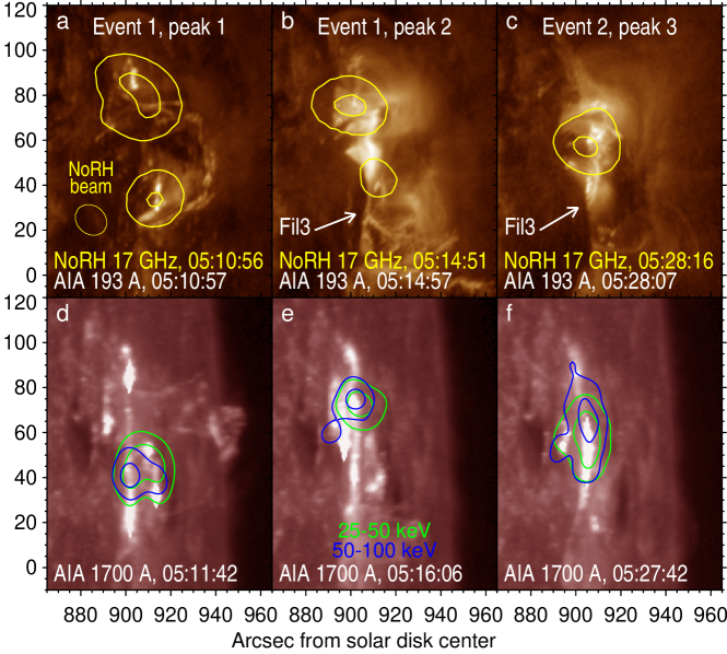
Figure 8.: Non-thermal manifestations in microwaves (top) and hard X-rays (bottom) at three main peaks in comparison with the structures observed in EUV. (a – c) Coronal 193 Å AIA images overlaid with 17 GHz NoRH images (yellow contours) at [$0.2,0.8$] of the maximum values. The thin yellow contour on panel a represents the NoRH beam at a half-height level. (d – f) Flare ribbons in 1700 Å AIA images along with RHESSI images at 25 – 50 keV (green contours) and 50 – 100 keV (blue contours) at [$0.3,0.7$] of the maximum values.F-hxr˙mw˙images

The AIA 1700 Å images (color background) in Figures F-hxr_mw_imagesd – F-hxr_mw_imagesf show the flare ribbons at the bases of the coronal arcades. These images are least distorted by saturation and do not correspond exactly to the times of the peaks. The HXR sources presented by the blue and green contours occupy sufficiently bright minor parts of the ribbons. An extended 50 – 100 keV source in Figure F-hxr_mw_images is almost as long as the middle ribbon R2. Smaller parts of the 50 – 100 keV sources correspond to ribbons R1 and R2, where magnetic fields were stronger than those beneath ribbon R2. Observations of extended ribbon-like structures in hard X-rays are exceptional (e.g. Masuda, Kosugi, and Hudson, 2001; Liu et al., 2007, 2013).

Masuda, Kosugi, and Hudson (2001) pointed out the limitations on the sensitivity and dynamic range (typically $\approx 10$) in the HXR imaging that Fourier-synthesis telescopes provide because of a limited coverage of the $(u,v)$-plane. Krucker et al. (2014) confirmed this conclusion for RHESSI; sources weaker than about 10 % of the brightest in an HXR image are not detectable. Thus, the simplicity and compactness of HXR sources that are usually observed result from instrumental limitations and do not reflect properties of non-thermal processes. Conversely, rare observations of ribbon-like HXR sources indicate some atypical conditions such as the uniformity of the magnetic-field strength or the uniformity of electron acceleration along the arcade (Liu et al., 2007).

Microwave and HXR images highlight different parts of the flare configuration, where accelerated electrons were present, but reveal them incompletely. The NoRH images at 17 GHz present unresolved sets of coronal loops, where magnetic field is sufficiently strong. Weaker-field regions are fainter at 17 GHz. With the power-law indices of the HXR spectra [$\gamma$] found in the next section, the emission at optically thin frequencies is expected to be highly dependent on the magnetic-field strength [$B$] as $B^{0.9\delta-0.22}\approx B^{4}$; $\delta=\gamma+1.5$ (Dulk and Marsh, 1982; White et al., 2011). Microwaves and hard X-rays dominate at different sides of an asymmetric magnetic configuration; the magnetic mirroring impedes electron precipitation (and hence the HXR emission) at the stronger-field side, where the optically thin gyrosynchrotron emission is stronger (Kundu et al., 1995).

These circumstances indicate that manifestations of accelerated electrons correspond to the structures observed in the EUV, but they are revealed incompletely because of instrumental limitations of RHESSI and NoRH. This result corresponds to the conclusions drawn previously by Zimovets, Kuznetsov, and Struminsky (2013) and Grechnev et al. (2017).

4.2 Hard X-Ray and Microwave Spectra

S-mw_spectra

The HXR spectra for the three temporal intervals corresponding to the main peaks were computed from RHESSI data using detectors 3 and 8 by means of the OSPEX package. The spectra in the 3 – 250 keV range have typical shapes that are consistent with a thermal core and non-thermal tail. The spectra were fitted with a thermal component at low energies and single power-law component at higher energies. Table T-spectra presents the accumulation-time intervals and parameters found for the spectra, the power-law index [$\gamma$] and the normalization constant [$A_{0}$] at a fiducial energy of 50 keV. The relations between the HXR spectra of the three peaks confirm the qualitative conclusions drawn in Section S-microwaves_HXR from the RHESSI temporal profiles presented in Figure F-time_prof.

Table 1.: Parameters of the HXR and microwave spectra.T-spectra

	Hard X-rays			Microwaves
	Accumulation	$A_{0}$[photons s-1 cm-2 keV-1]	$\gamma$	$N_{\mathrm{r}}$[$10^{7}$ electrons cm-3]	$\overline{|B|}$	$\nu_{\mathrm{peak}}$	$S_{\max}$
	time [UTC]	at 50 keV		$\geq 10$ keV	[G]	[GHz]	[sfu]
Peak 1	05:09:40–05:11:43	1.08	3.33	7.42	480	6.1	370
Peak 2	05:14:40–05:15:41	0.375	3.03	3.23	630	12.4	390
Peak 3	05:27:12–05:29:00	0.748	3.16	3.44	350	7.4	720

With the parameters found for the HXR spectra, it is possible to model the microwave spectra using the magnetogram actually observed. The most advanced modeling tool, of which we are aware, is the GX Simulator developed by Nita et al. (2015). In particular, this software allows one to model the gyrosynchrotron (GS) spectrum of an inhomogeneous source with various electron distributions based on a real magnetogram. However, the usage of the GX Simulator with a considerable number of loops seems to be difficult.

We invoke a different approach following Grechnev et al. (2017) who used a multi-loop model. The model contains a considerable number of pairs of homogeneous cubic GS sources in the legs of microwave-emitting loops rooted in the ribbons, each with a different magnetic-field strength and volume. In our flare, one of the legs of each loop is rooted in the middle ribbon. The total flux is the sum of the fluxes emitted by all of the loops, which are considered not to overlap with each other; thus, the number of the loops is about the ribbon length-to-width ratio (13 in our case). The number [$m$] of paired sources is chosen so that the sum of [$2m$] sources provides a smooth spectrum with single maximum and the modeled spectrum acceptably matches the observed fluxes measured at different frequencies. The model uses a simplified analytical description of the GS emission presented by Dulk and Marsh (1982). Using the radial magnetic-field distribution on the photosphere and the balance of magnetic fluxes in the conjugate legs of the loops, parameters of each source are estimated. Then, the magnetic-field strengths are corrected to the coronal values using a constant scaling factor that is estimated by referring to Lee, Nita, and Gary (2009). The model underestimates the low-frequency part of the spectrum that we disregard.

From the parameters of the HXR spectra for the three peaks that are listed in the middle part of Table T-spectra, we estimated the number $N_{\mathrm{r}}$ of microwave-emitting electrons per unit volume in the distribution above the fiducial electron energy $E_{\mathrm{r}}=10$ keV (Dulk and Marsh, 1982; White et al., 2011). The average magnetic-field strength in the coronal microwave sources $\overline{|B|}$, the peak frequency $\nu_{\mathrm{peak}}$ of the GS spectrum, and the maximum flux $S_{\max}$ at this frequency found in the modeling for each of the three peaks are listed in the right part of Table T-spectra. The magnetic-field strengths estimated in the modeling do not contradict the values found from the extrapolation in the potential-field approximation.

The spectra of the three peaks obtained in the modeling of 13 pairs of microwave sources are presented in Figure F-model_spectra along with the observed values (similar to Figure F-mw_spectra). The modeling acceptably reproduces the turnover part of the actual spectra and their adjacent branches between 2 and 17 GHz. The modeled spectra are underestimated at 2 GHz and lower frequencies (not shown). It is only possible to state that the modeled spectra do not contradict the fluxes estimated at 34 GHz, because their uncertainties are large. A formal increase in the number of sources does not bring the modeled spectra closer to the observations.

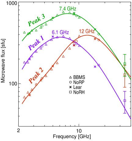
Figure 9.: Gyrosynchrotron spectra modeled for the three main peaks (color curves). The symbols represent the actual measurements (same as in Figure F-mw_spectra). F-model˙spectra

The modeling confirms that microwaves were emitted in coronal loops by the same electron populations, whose precipitation produced hard X-rays in both flares, although the spatial separation between the HXR and microwave sources was considerable. The low-frequency flattening of the microwave spectra was caused by the asymmetry of the magnetic configuration. The challenging shift of the spectral turnover to the left-up from peak 2 to peak 3 was a result of an increased asymmetry in the second flare. The modeling also confirms that apparently simple microwave sources observed by NoRH at 17 GHz actually represented two flare arcades. Manifestations of accelerated electrons in microwaves correspond to the structures observed in the EUV indeed.

5 Summary and Concluding Remarks

S-conclusion

Having got a pointing from SRH at two major flares, which occurred within half an hour in the same active region and exhibited different emission spectra, we analyzed the twin events using EUV, hard X-ray, and microwave data along with magnetograms. Both events were eruptive flares, each of which had an unusual three-ribbon configuration. The events led to a CME, whose structure indicated its origin due to the twin eruptions.

The magnetic configuration, where the events occurred, was characterized by a considerable excess of the S-polarity magnetic flux over the N-polarity flux in an extended plage region. The excessive S-polarity flux high above the plage region was concentrated within a tube-like outer spine that was rooted in a remote N-polarity sunspot. The coronal configuration just above the plage region had a shape of an inverted funnel that contained a null point in the waist. Because of the extended geometry, the funnel and the null-point region were stretched along the solar surface parallel to the plage region.

Each of the two magnetic domains inside the funnel contained a filament before the events. The filaments erupted one after another within half an hour. A scenario was inferred from multi-spectral observations that combines the twin events in terms of null-point-associated successive eruptions. Each rising filament moved to the null-field region that inevitably resulted in partial reconnection between the erupting structure and static coronal environment. Two successive flares developed in this way that basically resembled circular-ribbon flares with the following modifications: The central brightening extended into the middle ribbon located in the N-polarity plage region and the circular ribbon transformed into two ribbons located in S-polarity magnetic fields on both sides of the middle ribbon. Thus, a three-ribbon flare configuration appeared. In this scenario, the first filament eruption facilitates the second.

The two flares produced considerable microwave, hard X-ray, and $\gamma$-ray bursts that are detectable at energies exceeding 800 keV. Microwave and hard X-ray images highlighted different parts of the flare configuration, where accelerated electrons were present. Hard X-ray sources occupied minor parts of the ribbons that were sufficiently bright in the EUV. An extended hard X-ray source in the second flare was almost as long as the middle ribbon. Two microwave sources that resembled two footpoints of a single loop represented in fact two different arcades that is confirmed by the modeling of microwave spectra. Manifestations of accelerated electrons in hard X-rays and microwaves corresponded to the structures observed in the EUV, but they were revealed incompletely because of instrumental limitations of RHESSI and NoRH.

The results indicate that the spatial resolution achievable in microwave observations, which are currently available, may be insufficient to discern flaring structures. On the other hand, the dynamic range of hard X-ray imagers may be insufficient to reveal the structures of hard X-ray sources perfectly. Hence, higher-resolution images with a sufficient dynamic range obtained in different spectral domains should be invoked for a correct interpretation of non-thermal flare sources.

Acknowledgments

We thank L.K. Kashapova for useful discussions. We appreciate our colleagues from the Radio Astrophysical Department and the Radio Astrophysical Observatory in Badary. This study was funded by the Russian Science Foundation under grant 18-12-00172. The development of the methods used in Sections S-microwaves_HXR and S-acc_electrons was supported by the Program of Basic Research of the RAS Presidium No. 28. The SRH and BBMS data were obtained using the Unique Research Facility Siberian Solar Radio Telescope (ckp-rf.ru/usu/73606).

We thank the NASA/SDO and the AIA and HMI science teams, the teams operating RHESSI, the Nobeyama solar facilities, and the US AF RSTN network for the data used here. We thank the International Consortium for the continued operation of Nobeyama Radioheliograph until shut down on 31 March 2020. We are grateful to the team maintaining the CME Catalog at the CDAW Data Center by NASA and the Catholic University of America in cooperation with the Naval Research Laboratory.

Disclosure of Potential Conflicts of Interest

The authors declare that they have no conflicts of interest.

References

- Aulanier, Janvier, and Schmieder (2012) Aulanier, G., Janvier, M., Schmieder, B.: 2012, The standard flare model in three dimensions. I. Strong-to-weak shear transition in post-flare loops. A&A 543, A110. DOI. ADS.
- Bamba et al. (2017) Bamba, Y., Inoue, S., Kusano, K., Shiota, D.: 2017, Triggering process of the X1.0 three-ribbon flare in the great active region NOAA 12192. ApJ 838(2), 134. DOI. ADS.
- Carmichael (1964) Carmichael, H.: 1964, A process for flares 50, NASA, Science and Technical Information Division, Washington DC, 451. ADS.
- Chandra et al. (2018) Chandra, R., Chen, P.F., Joshi, R., Joshi, B., Schmieder, B.: 2018, Observations of two successive EUV waves and their mode conversion. ApJ 863(1), 101. DOI. ADS.
- Dulk and Marsh (1982) Dulk, G.A., Marsh, K.A.: 1982, Simplified expressions for the gyrosynchrotron radiation from mildly relativistic, nonthermal and thermal electrons. ApJ 259, 350. DOI. ADS.
- Filippov (1999) Filippov, B.: 1999, Observation of a 3d magnetic null point in the solar corona. Sol. Phys. 185(2), 297. DOI. ADS.
- Filippov, Golub, and Koutchmy (2009) Filippov, B., Golub, L., Koutchmy, S.: 2009, X-ray jet dynamics in a polar coronal hole region. Sol. Phys. 254, 259. DOI. ADS.
- Grechnev et al. (2005) Grechnev, V.V., Chertok, I.M., Slemzin, V.A., Kuzin, S.V., Ignat’ev, A.P., Pertsov, A.A., Zhitnik, I.A., Delaboudinière, J.-P., Auchère, F.: 2005, CORONAS-F/SPIRIT EUV observations of October-November 2003 solar eruptive events in combination with SOHO/EIT data. J. Geophys. Res. (Space Physics) 110, A09S07. DOI. ADS.
- Grechnev et al. (2006) Grechnev, V.V., Uralov, A.M., Zandanov, V.G., Baranov, N.Y., Shibasaki, K.: 2006, Observations of prominence eruptions with two radioheliographs, SSRT, and NoRH. PASJ 58, 69. DOI. ADS.
- Grechnev et al. (2008) Grechnev, V.V., Uralov, A.M., Slemzin, V.A., Chertok, I.M., Kuzmenko, I.V., Shibasaki, K.: 2008, Absorption phenomena and a probable blast wave in the 13 July 2004 eruptive event. Sol. Phys. 253(1-2), 263. DOI. ADS.
- Grechnev et al. (2011a) Grechnev, V.V., Uralov, A.M., Chertok, I.M., Kuzmenko, I.V., Afanasyev, A.N., Meshalkina, N.S., Kalashnikov, S.S., Kubo, Y.: 2011a, Coronal shock waves, EUV waves, and their relation to CMEs. I. Reconciliation of “EIT waves”, Type II radio bursts, and leading edges of CMEs. Sol. Phys. 273, 433. DOI. ADS.
- Grechnev et al. (2011b) Grechnev, V.V., Kuzmenko, I.V., Chertok, I.M., Uralov, A.M.: 2011b, Solar flare-related eruptions followed by long-lasting occultation of the emission in the He II 304 Å line and in microwaves. Astron. Rep. 55, 637. DOI. ADS.
- Grechnev et al. (2013a) Grechnev, V.V., Kiselev, V.I., Uralov, A.M., Meshalkina, N.S., Kochanov, A.A.: 2013a, An updated view of solar eruptive flares and the development of shocks and CMEs: History of the 2006 December 13 GLE-productive extreme event. PASJ 65, S9. DOI. ADS.
- Grechnev et al. (2013b) Grechnev, V.V., Kuz’menko, I.V., Uralov, A.M., Chertok, I.M., Kochanov, A.A.: 2013b, Microwave negative bursts as indications of reconnection between eruptive filaments and a large-scale coronal magnetic environment. PASJ 65, S10. DOI. ADS.
- Grechnev et al. (2014) Grechnev, V.V., Uralov, A.M., Slemzin, V.A., Chertok, I.M., Filippov, B.P., Rudenko, G.V., Temmer, M.: 2014, A challenging solar eruptive event of 18 November 2003 and the causes of the 20 November geomagnetic superstorm. I. Unusual history of an eruptive filament. Sol. Phys. 289, 289. DOI. ADS.
- Grechnev et al. (2015) Grechnev, V.V., Uralov, A.M., Kuzmenko, I.V., Kochanov, A.A., Chertok, I.M., Kalashnikov, S.S.: 2015, Responsibility of a filament eruption for the initiation of a flare, CME, and blast wave, and its possible transformation into a bow shock. Sol. Phys. 290, 129. DOI. ADS.
- Grechnev et al. (2016) Grechnev, V.V., Uralov, A.M., Kochanov, A.A., Kuzmenko, I.V., Prosovetsky, D.V., Egorov, Y.I., Fainshtein, V.G., Kashapova, L.K.: 2016, A tiny eruptive filament as a flux-rope progenitor and driver of a large-scale CME and wave. Sol. Phys. 291, 1173. DOI. ADS.
- Grechnev et al. (2019) Grechnev, V.V., Kochanov, A.A., Uralov, A.M., Slemzin, V.A., Rodkin, D.G., Goryaev, F.F., Kiselev, V.I., Myshyakov, I.I.: 2019, Development of a fast CME and properties of a related interplanetary transient. Sol. Phys. 294(10), 139. DOI. ADS.
- Grechnev et al. (2017) Grechnev, V., Uralov, A.M., Kiselev, V.I., Kochanov, A.A.: 2017, The 26 December 2001 solar eruptive event responsible for GLE63. II. Multi-loop structure of microwave sources in a major long-duration flare. Sol. Phys. 292(1), 3. DOI. ADS.
- Guidice (1979) Guidice, D.A.: 1979, Sagamore Hill radio observatory, Air Force geophysics laboratory, Hanscom Air Force base, Massachusetts 01731. Report. BAAS 11, 311. ADS.
- Guidice et al. (1981) Guidice, D.A., Cliver, E.W., Barron, W.R., Kahler, S.: 1981, The Air Force RSTN system. BAAS 13, 553. ADS.
- Hansen, Tripathi, and Bellan (2004) Hansen, J.F., Tripathi, S.K.P., Bellan, P.M.: 2004, Co- and counter-helicity interaction between two adjacent laboratory prominences. Physics of Plasmas 11(6), 3177. DOI. ADS.
- Hirayama (1974) Hirayama, T.: 1974, Theoretical model of flares and prominences. I: Evaporating flare model. Sol. Phys. 34(2), 323. DOI. ADS.
- Inhester, Birn, and Hesse (1992) Inhester, B., Birn, J., Hesse, M.: 1992, The evolution of line tied coronal arcades including a converging footpoint motion. Sol. Phys. 138(2), 257. DOI. ADS.
- Janvier et al. (2013) Janvier, M., Aulanier, G., Pariat, E., Démoulin, P.: 2013, The standard flare model in three dimensions. III. Slip-running reconnection properties. A&A 555, A77. DOI. ADS.
- Kashapova et al. (2013) Kashapova, L.K., Tokhchukova, S.K., Zhdanov, D.A., Bogod, V.M., Rudenko, G.V.: 2013, The subsecond pulses during the August 10, 2011 flare by observations of RATAN-600 and the 4-8 GHz Siberian solar spectropolarimeter. Geomag. Aeron. 53(8), 1021. DOI. ADS.
- Kochanov et al. (2013) Kochanov, A.A., Anfinogentov, S.A., Prosovetsky, D.V., Rudenko, G.V., Grechnev, V.V.: 2013, Imaging of the solar atmosphere by the Siberian Solar Radio Telescope at 5.7 GHz with an enhanced dynamic range. PASJ 65, S19. DOI. ADS.
- Kopp and Pneuman (1976) Kopp, R.A., Pneuman, G.W.: 1976, Magnetic reconnection in the corona and the loop prominence phenomenon. Sol. Phys. 50(1), 85. DOI. ADS.
- Krucker et al. (2014) Krucker, S., Christe, S., Glesener, L., Ishikawa, S.-n., Ramsey, B., Takahashi, T., Watanabe, S., Saito, S., Gubarev, M., Kilaru, K., et al.: 2014, First images from the Focusing Optics X-Ray Solar Imager. ApJ 793(2), L32. DOI. ADS.
- Kundu et al. (1995) Kundu, M.R., Nitta, N., White, S.M., Shibasaki, K., Enome, S., Sakao, T., Kosugi, T., Sakurai, T.: 1995, Microwave and hard X-ray observations of footpoint emission from solar flares. ApJ 454, 522. DOI. ADS.
- Lee, Nita, and Gary (2009) Lee, J., Nita, G.M., Gary, D.E.: 2009, Electron energy and magnetic field derived from solar microwave burst spectra. ApJ 696(1), 274. DOI. ADS.
- Lemen et al. (2012) Lemen, J.R., Title, A.M., Akin, D.J., Boerner, P.F., Chou, C., Drake, J.F., Duncan, D.W., Edwards, C.G., Friedlaender, F.M., Heyman, G.F., et al.: 2012, The Atmospheric Imaging Assembly (AIA) on the Solar Dynamics Observatory (SDO). Sol. Phys. 275, 17. DOI. ADS.
- Lesovoi and Kobets (2017) Lesovoi, S., Kobets, V.: 2017, Correlation plots of the Siberian Radioheliograph. Solar-Terr. Phys. 3(1), 19. DOI. ADS.
- Lesovoi et al. (2014) Lesovoi, S.V., Altyntsev, A.T., Ivanov, E.F., Gubin, A.V.: 2014, A 96-antenna radioheliograph. Res. Astron. Astrophys. 14, 864. DOI. ADS.
- Lesovoi et al. (2017) Lesovoi, S., Altyntsev, A., Kochanov, A., Grechnev, V., Gubin, A., Zhdanov, D., Ivanov, E., Uralov, A., Kashapova, L., Kuznetsov, A., Meshalkina, N., Sych, R.: 2017, Siberian Radioheliograph: First results. Solar-Terr. Phys. 3(1), 3. DOI. ADS.
- Lin et al. (2002) Lin, R.P., Dennis, B.R., Hurford, G.J., Smith, D.M., Zehnder, A., Harvey, P.R., Curtis, D.W., Pankow, D., Turin, P., Bester, M., et al.: 2002, The Reuven Ramaty High-Energy Solar Spectroscopic Imager (RHESSI). Sol. Phys. 210, 3. DOI. ADS.
- Liu et al. (2007) Liu, C., Lee, J., Gary, D.E., Wang, H.: 2007, The ribbon-like hard X-ray emission in a sigmoidal solar active region. ApJ 658(2), L127. DOI. ADS.
- Liu et al. (2013) Liu, C., Deng, N., Lee, J., Wiegelmann, T., Moore, R.L., Wang, H.: 2013, Evidence for solar tether-cutting magnetic reconnection from coronal field extrapolations. ApJ 778(2), L36. DOI. ADS.
- Longcope and Beveridge (2007) Longcope, D.W., Beveridge, C.: 2007, A quantitative, topological model of reconnection and flux rope formation in a two-ribbon flare. ApJ 669(1), 621. DOI. ADS.
- Masson et al. (2009) Masson, S., Pariat, E., Aulanier, G., Schrijver, C.J.: 2009, The nature of flare ribbons in coronal null-point topology. ApJ 700, 559. DOI. ADS.
- Masson et al. (2017) Masson, S., Pariat, É., Valori, G., Deng, N., Liu, C., Wang, H., Reid, H.: 2017, Flux rope, hyperbolic flux tube, and late extreme ultraviolet phases in a non-eruptive circular-ribbon flare. A&A 604, A76. DOI. ADS.