The Nonstandard Properties of a “Standard” PWN: Unveiling the Mysteries of PWN   Using its IR and X-ray emission

Abstract

The evolution of a pulsar wind nebula (PWN) depends on properties of the progenitor star, supernova, and surrounding environment. As some of these quantities are difficult to measure, reproducing the observed dynamical properties and spectral energy distribution (SED) with an evolutionary model is often the best approach in estimating their values. , powered by the pulsar J1833$-$1034, is a well observed PWN for which previous modeling efforts have struggled to reproduce the observed SED. In this study, we reanalyze archival infrared (IR; Herschel, Spitzer) and X-ray (Chandra, NuSTAR, Hitomi) observations. The similar morphology observed between IR line and continuum images of this source indicates that a significant portion of this emission is generated by surrounding dust and gas, and not synchrotron radiation from the PWN. Furthermore, we find the broadband X-ray spectrum of this source is best described by a series of power laws fit over distinct energy bands. For all X-ray detectors, we find significant softening and decreasing unabsorbed flux at higher energy bands. Our model for the evolution of a PWN is able to reproduce the properties of this source when the supernova ejecta has a low initial kinetic energy $E_{\mathrm{sn}}\approx 1.2\times 10^{50}\,\mathrm{ergs}$ and the spectrum of particles injected into the PWN at the termination shock is softer at low energies. Lastly, our hydrodynamical modeling of the SNR can reproduce its morphology if there is a significant density increase of the ambient medium ${\sim}1.8$ pc north of the explosion center.

1 Introduction

Stars with mass in the range $M\gtrsim 8~{}M_{\odot}$ are believed to end their lives in a core-collapse supernova event (Baade & Zwicky 1934). In many cases, this produces a highly magnetized and rapidly rotating neutron star (i.e., pulsar). Pulsar’s dissipate their rotational energy by powering a relativistic outflow of electrons and positrons, commonly referred to as the “pulsar wind”. The expanding magnetic bubble of particles, created by the interaction of the relativistic pulsar wind with the ambient medium, is the pulsar wind nebula (PWN). For young PWNe the ambient medium is the slow-moving supernova ejecta in the host supernova remnant (SNR), but for older PWNe it can also be interstellar medium (ISM) after the pulsar exits the SNR (Slane, 2017). The reader is directed to Slane (2017), Gaensler & Slane (2006), Chevalier (2005), Arons (2004), and Amato (2020) for detailed explanations on PWNe.

As the evolution of a PWN depends on the central neutron star, the composition of the pulsar wind, and its surrounding environment, modeling PWNe allows us to determine the physical characteristics of all components of the system–which are difficult, if not impossible, to determine by other means (e.g., Torres 2017). In addition, evolutionary models allow us to infer properties of the progenitor star and supernova. Furthermore, such models also determine the spectrum of particles accelerated inside these sources, needed to determine the currently unknown physical mechanism (Sironi et al., 2013) by which such objects produce some of the most energetic particles observed in the Universe. The modeling is done by generating the dynamical properties and spectral energy distribution (SED) which can be fit against measurements gathered over the entire electromagnetic spectrum.

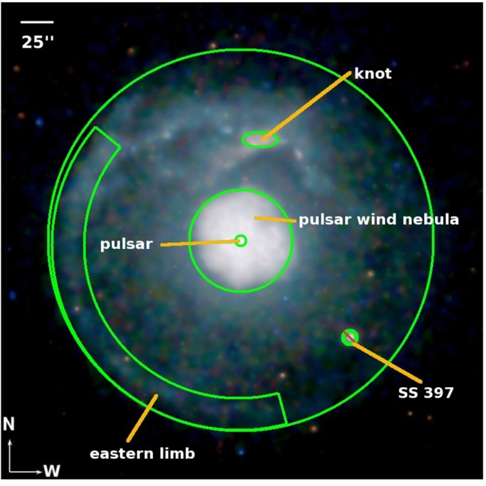
Figure 1: Image of  with the individual components labeled. Reproduced from Matheson & Safi-Harb (2010).

PWN  is a bright X-ray emitting source well-suited for modeling as it has been observed by many telescopes spanning the electromagnetic spectrum. Initially detected in 1970 (Altenhoff et al. 1970; Wilson & Altenhoff 1970) in the radio band and later observed in the X-ray band in 1981 (Becker & Szymkowiak, 1981), its central pulsar J1833$-$1034 was detected in 2006 (Camilo et al., 2006) whose measured period $P$ and period-derivative $\dot{P}$ suggest a high spin-down luminosity and a low characteristic age. As a PWN with a circular morphology (Figure 1) associated with a young ($\lesssim 10^{4}$ years) pulsar,  is appropriate for an analysis using “one-zone” models (e.g., Reynolds & Chevalier 1984, see Gelfand 2017 for a recent review).

Table 1: Previous broken power-law measurements of the X-ray spectrum of PWN

Observatory	Energy Range	$N_{H}$	$\Gamma_{1}$	$E_{\rm break}$	$\Gamma_{2}$	$F_{2-8}$	$F_{15-50}$
$\cdots$	[keV]	[$10^{22}$ cm-2]	$\cdots$	[keV]	$\cdots$	[$10^{-11}~{}\frac{\rm erg}{\rm cm^{2}~{}s}$]	[$10^{-11}~{}\frac{\rm erg}{\rm cm^{2}~{}s}$]
NuSTAR	3$-$45	$\equiv 2.99$	$1.996_{-0.012}^{+0.013}$	$9.1_{-1.4}^{+1.2}$	$2.093_{-0.012}^{+0.013}$	$5.27\pm 0.08$	$5.11\pm 0.08$
Hitomi	0.8$-$80	$3.22\pm 0.03$	$1.74\pm 0.02$	$7.1\pm 0.3$	$2.14\pm 0.01$	$4.80\pm 0.02$	$4.54\pm 0.04$

Note: The NuSTAR results are from Nynka et al. (2014) and the Hitomi results are from Hitomi Collaboration et al. (2018). $F_{2-8}$ indicates the $2-8$ keV flux and $F_{15-50}$ indicates the $15-50$ keV flux. Errors are 90% confidence intervals.

However, previous attempts to model this system have not succeeded in simultaneously reproducing the radio and X-ray spectrum (Tanaka & Takahara, 2011; Torres et al., 2014; Hitomi Collaboration et al., 2018). The modeling is further complicated by the discrepant measurement of the X-ray spectrum by three observatories, Chandra, NuSTAR, and Hitomi (Guest et al., 2019; Nynka et al., 2014; Hitomi Collaboration et al., 2018). One such difference is shown in Table 1, where the parameters for the broken power-law model between NuSTAR and Hitomi are in disagreement. Furthermore, the infrared (IR) emission observed from this source (Gallant & Tuffs, 1999), often assumed to be dominated by synchrotron radiation from the PWN (e.g., Tanaka & Takahara 2011; Torres et al. 2014; Hitomi Collaboration et al. 2018), may be contaminated by emission from surrounding gas and dust. To address these concerns, we reanalyzed archival IR and X-ray observations of this source.

This paper is structured as follows. In §2 we describe the IR and X-ray observations and detector-specific data reduction and analysis of PWN . In §3 we describe our piecewise power-law fitting approach to analyze the X-ray spectra and present our results. In §4 we discuss the implications of these results in our modeling for this source. We summarize our findings in §5.

2 Observations and Data Analysis

In this section, we describe our analysis of archival IR (Herschel, Spitzer §2.1) and X-ray (Chandra §2.2, NuSTAR §2.3, and Hitomi §2.4) observations of this source.

2.1 Infrared Observations

was observed with the Photodetector Array Camera (PACS) Integral Field Unit Spectrometer (Poglitsch et al., 2010) aboard Herschel Space Observatory on 2013 April 07. The range spectroscopy mode was used to cover the [O I] 63.2 $\mu$m and 145.5 µm, [O III] 88.4 $\mu$m, and [C II] 157.7 $\mu$m emission lines. The total field of view of one IFU pointing is $47\arcsec\ \times 47\arcsec$, consisting of 25 spaxels. In order to cover the entire PWN in   we obtained a 2 $\times$ 2 mosaic IFU mosaic of the source, as well as a single-pointing off-source background observation for each line. The IFU cubes were analyzed using HIPE version 15.0.1 (Ott, 2010). The analysis included trimming of the spectral edges and a subtraction of the baseline continuum obtained by a 2-degree polynomial fit across the line-free spectral region. While narrow background lines were detected in the baseline-subtracted and spatially-integrated spectrum of the off-source IFU pointing, both narrow and broad lines were detected in the IFU cubes centered on the PWN. The broad lines have a full-width-at-half-maximum (FWHM) of 850 ${\rm km\>s}^{-1}$ for the [C II] 157.7 $\mu$m µm and 1000 ${\rm km\>s}^{-1}$ for the [O I] 63.2 $\mu$m 63.2 µm line and likely arise from SN ejecta material. The corresponding ejecta velocities are then 425$\pm$75 ${\rm km\>s}^{-1}$ and 500$\pm$20 ${\rm km\>s}^{-1}$ for the [C II] 157.7 $\mu$m and [O I] 63.2 $\mu$m, respectively. If the observed line emission arises predominantly from ejecta with a low tangential velocity, the expansion velocity measured from the lines would represent a lower limit on the true velocity, which could be up to a factor of two higher, giving an expansion velocity range between 350 and 1000 ${\rm km\>s}^{-1}$. In a radiative shock, the emission that we observe likely arises from highest-density material at the contact discontinuity, in which case the observed velocity represent the expansion velocity of the PWN rather than the free expansion velocity of the ejecta. However, since the shock velocities that produce the IR lines are relatively low, the free-expansion velocity of the ejecta material at the PWN boundary is within a similar range.

We produced emission line maps of the [O I] 63.2 $\mu$m and [C II] 157.7 $\mu$m ejecta lines by integrating the spectra across the broad-line component, while excluding the narrow line that arises from the background emission. The maps are shown in Figure 2 with the X-ray contours from the PWN overlaid in white.

Total IR flux densities of the PWN region in  were estimated from the images obtained with the Infrared Array Camera (IRAC) and Multiband Imaging Photometer (MIPS) aboard Spitzer (PID 3647, PI: Slane), and the Photodetector Array Camera and Spectrometer (PACS) and Spectral and Photometric Imaging REceiver (SPIRE) instruments aboard Herschel (Obs ID 1342218642), spanning a wavelength range between 3.6 and 500 µm. For the MIPS, PACS, and SPIRE images, we extracted the total flux densities using an aperture centered on the PWN with a radius of 41.5″ and a background annulus with inner and outer radii of 41.5″ and 74.0″, respectively. The IR images and the extraction aperture are shown in Figure 3 and total flux densities listed in Table 2. The uncertainties on the flux densities in this case are dominated by the uncertainties of the local background emission. The IRAC images show very faint emission from the PWN, superposed on a dense stellar field. To make a rough estimate of the PWN emission in the IRAC bands, we estimated the surface brightness in a very small region free of stellar sources and assumed that this surface brightness is constant across the entire area of the PWN. The estimated background-subtracted surface brightness values at 3.6, 4.5, 5.8, and 8.0 µm are 0.33, 0.37, 1.6, and 4.0 MJy/sr. The total flux densities were estimated by multiplying by a PWN area of $8.7\times 10^{-8}$ steradians.

Table 2: Observed (§2.1) and Predicted synchrotron (§4.2) IR flux density of the PWN

Instrument Wavelength $\lambda$ Total Flux Density $S_{\nu}^{\rm tot}$ PWN Flux density $S_{\nu}^{\rm pwn}$ Residual Flux Density $S_{\nu}^{\rm resid}$ Variable $p$ $p\equiv 1.85690$ Variable $p$ $p\equiv 1.85690$ (µm) (Jy) (Jy) (Jy) (Jy) (Jy) SPIRE 500 1.0$\pm$0.2 0.64 0.67 0.36 0.33 SPIRE 350 1.2$\pm$0.2 0.48 0.50 0.72 0.70 SPIRE 250 1.6$\pm$0.2 0.35 0.37 1.25 1.23 PACS 160 3.7$\pm$1.0 0.21 0.22 3.49 3.48 PACS 70 3.4$\pm$1.5 0.11 0.11 3.29 3.29 MIPS 24 0.22$\pm$0.03 0.037 0.039 0.183 0.181 IRAC 8.0 $\sim$0.33 0.014 0.015 0.316 0.315 IRAC 5.8 $\sim$0.13 0.011 0.011 0.119 0.119 IRAC 4.5 $\sim$0.031 0.009 0.009 0.022 0.022 IRAC 3.6 $\sim$0.027 0.007 0.008 0.020 0.019

Figure 2: Emission line maps of the O I 63.2 µm and C II 157.7 µm broad ejecta lines in the PWN region are shown in the left and middle panels, respectively. The MIPS 24 µm image of the same region is shown in the right panel. The X-ray contours from the PWN are shown in white.

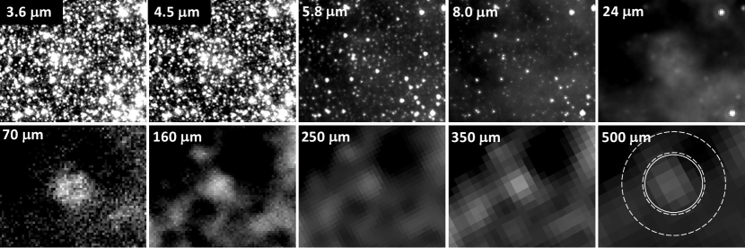
Figure 3: The Spitzer 3.6, 4.5, 5.8, 8.0, and 24 µm images and Herschel 70, 160, 250, 350, and 500 µm images of the PWN region in SNR . The last panel shows the extraction aperture and background annulus used to extract the total flux densities in the Spitzer 24 µm image and all the Herschel images. The corresponding flux densities are listed in Table 2.

2.2 Chandra Observations

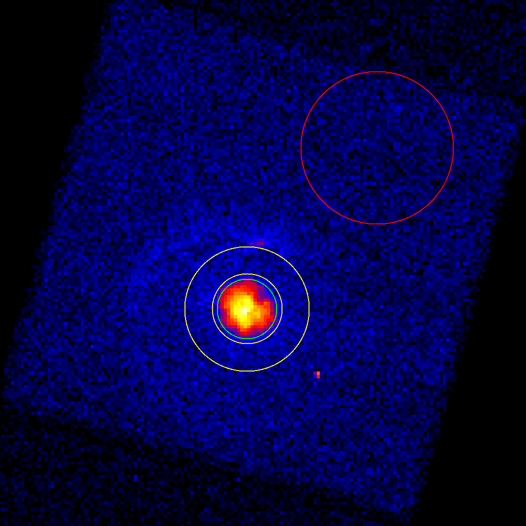
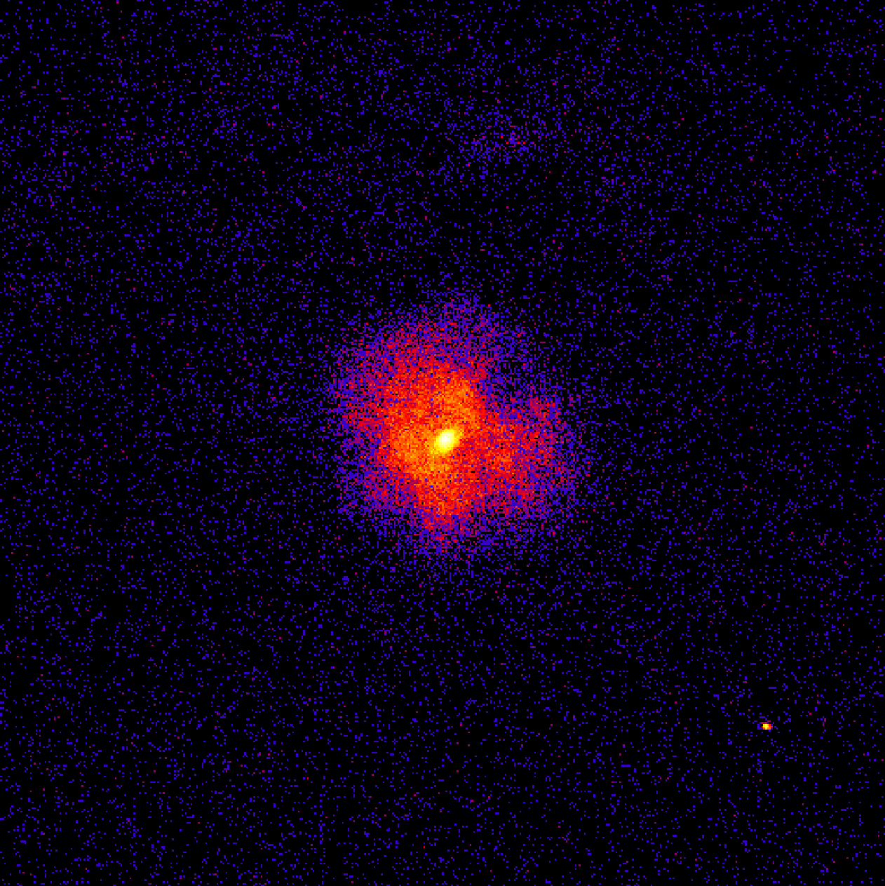
Figure 4: Chandra images of . Images are taken from ObsID 1433 (Table 3). Left: Image showing the Chandra source region (green), the Chandra background region (red), and the IR background annulus (yellow). Right: An enlarged view of the PWN.

Chandra has regularly observed  with both its Advanced CCD Imaging Spectrometer (ACIS) and High Resolution Camera (HRC). For this study we reanalyzed ACIS-S observations where  fell on the S3 chip, the back-illuminated chip where the best imaging and energy resolution is obtained. A single ACIS chip has a field of view of $8.3\arcmin\times 8.3\arcmin$ with an imaging resolution of $\sim 1\arcsec$ over the energy range 0.2–10 keV.

Software used for this analysis include CIAO version 4.10 (Fruscione et al., 2006) and its accompanying Sherpa version (Freeman et al., 2001; Doe et al., 2007), as well as SAOImage DS9 version 7.6 (Joye & Mandel, 2003; Smithsonian Astrophysical Observatory, 2000).

After querying and downloading 16 ACIS-S observations from the Chandra Data Archive where  fell on the S3 chip, error-causing subarray files (ObsIDs 1554, 3693, 10646, 14263, 16420) were deleted.

After analyzing each observation independently, we found that the results for ObsIDs 1230 and 159 deviated significantly from those for all other ObsIDs. Upon investigation, this discrepancy was attributed to these observations being taken with focal plane temperatures of -$100^{\circ}$C, as compared with -$110^{\circ}$C or -$120^{\circ}$C focal plane temperatures for all the other observations. The accuracy of the temperature-dependent gain correction decreases for temperatures below -$112^{\circ}$C, so ObsIDs 1230 and 159 were deemed too warm to provide reliable spectral results.

Spectra were extracted for the stack of all 11 remaining observations, summarized in Table 3, over the energy band 0.5-8 keV using the CIAO tool specextract. These spectra were extracted using a $35\arcsec$ radius circular region covering the entire central PWN as shown in Figure 4.

Table 3: Details of Chandra observations

ObsID	Start Time	Data Mode	Exposure [s]
1433	1999-11-15 22:31:18	FAINT	14970
1717	2000-05-23 09:24:15	FAINT	7540
1770	2000-07-05 03:42:36	FAINT	7220
1838	2000-09-02 01:09:11	FAINT	7850
2873	2002-09-14 01:09:17	FAINT	9830
3700	2003-11-09 12:20:43	VFAINT	9540
5159	2004-10-27 13:32:57	VFAINT	9830
5166	2004-03-14 22:12:41	VFAINT	10020
6071	2005-02-26 09:08:53	VFAINT	9640
6741	2006-02-22 02:57:52	VFAINT	9830
8372	2007-05-25 12:06:03	VFAINT	10010

2.3 NuSTAR Observations and Data Reduction

The Nuclear Spectroscopic Telescope Array (NuSTAR) is a high-energy (3-79 keV) X-ray space observatory consisting of two co-aligned telescopes with detectors placed at each of their focal plane modules (referred to as FPMA and FPMB) (Harrison et al., 2013). Each NuSTAR telescope has a field of view of $12\arcmin\times 12\arcmin$ with a full-width half maximum (FWHM) of $18\arcsec$ and a half-power diameter (HPD) of $58\arcsec$. The FWHM spectral resolution is 400 eV at 10 keV. NuSTAR observed  on nine separate occasions for a total of $\sim$383 ks on each of its two on-board FPM detectors (see Table 4). Of the nine observations, two of them (ObsID 10002014001, 40001016001) were taken in the STELLAR spacecraft mode, making them unsuitable for science observations due to the spacecraft roll maneuver of $\sim$1 deg/day as mentioned in the NuSTAR Master Catalog. As such, we did not analyze these observations. In addition, due to the short effective exposure time of ObsID 10002014006, we did not analyze this observation. Of the remaining six observations, the previous (Nynka et al., 2014) paper analyzed four observations (ObsID 10002014003, 10002014004, 40001016002, 40001016003) totalling $\sim$190 ks, but did not analyze two observations (ObsID 10002014002, 10002014005) which would add an additional $\sim$178 ks. We analyzed six observations, including the two previously unanalyzed observations, for a total exposure time of $\sim$368 ks on each FPM. As each observation was done by both detectors on NuSTAR, we analyzed a total of twelve data-sets.

For all twelve data-sets we followed the standard pipeline processing (HEASoft v6.24 (NASA High Energy Astrophysics Science Archive Research Center (2014), HEASARC) and NuSTARDAS v1.80) as explained in the NuSTAR Data Analysis Software Guide prior to spectral fitting. We ran the processing script nupipeline (v0.4.6) with the default options to produce the cleaned and calibrated event files, referred to as “Level 2 Data Products” in the guide. The default pipeline option does not perform any South Atlantic Anomaly (SAA) filtering (done via the command nucalcsaa). While the SAA filter may be required for fainter sources,  is a relatively bright source ($>$1 count per second) and therefore there is likely no need for SAA filtering as mentioned in the official NuSTAR website (Background Filtering).

Once the cleaned and calibrated event files were created, we generated the associated redistribution/response matrix (RMF) and ancillary response (ARF) files by running nuproducts (v0.3.3) with the option extended=yes. The extended=yes option is necessary to generate the ARF appropriate for an extended source.

The source spectra was extracted using a $177\arcsec$ radius circular region centered on the PWN and the background spectra were extracted using two rectangular regions away from the source Figure 5. This conventional background extraction method may induce small uncertainties/fluctuations in the background as the NuSTAR background is known to be non-uniform across it’s field of view (Wik et al., 2014). However, since  is roughly 10 times brighter than the background in most of the energy range we do spectral fitting for these background uncertainties should be negligible. We also see no stray light emission from nearby bright X-ray sources in the field of view that may contribute to the background during any of the observations. We confirmed that stray light is not an issue during the observations of this source using the NuSTAR Science Operation Center’s NuSTAR constraint check page.

Table 4: NuSTAR Observations of  

ObsID	Start Time	Obs Type	Spacecraft Mode	Exposure A [s]	Exposure B [s]
10002014001	2012-07-27 14:36:07	CAL	STELLAR	12990	13003
10002014002	2012-07-28 01:01:07	CAL	INERTIAL	44456	44447
10002014003	2012-07-29 01:21:07	CAL	INERTIAL	44723	44722
10002014004	2012-07-30 01:33:37	CAL	INERTIAL	28023	28011
10002014005	2012-07-31 19:38:33	CAL	INERTIAL	133782	133760
10002014006	2012-08-03 20:51:07	CAL	INERTIAL	1944	1956
40001016001	2013-02-26 05:31:07	SNR	STELLAR	50	50
40001016002	2013-02-26 05:56:07	SNR	INERTIAL	29704	29679
40001016003	2013-02-26 22:11:07	SNR	INERTIAL	87721	87646

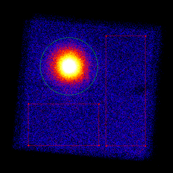
Figure 5: A representative NuSTAR image of  with the source and background region used for the spectral analysis described in §2.3. The green circle is the source region and the two red rectangles are the background regions. While NuSTAR has two on-board detectors, the images between the two detectors for this source at the given observations were nearly identical.

Figure 6: Hitomi detector images of . From left to right, the SXI and both HXI detectors are shown. In the SXI image the source region is shown as the innermost circle. The background region is shown as the white square where the source region, a larger annulus around the source, and previously known X-ray point sources in the FoV are excluded. In the HXI images the source region is shown as the white circle and the background region by the green rectangle where the source region is excluded. Source and background regions are taken from the Hitomi step by step analysis guide version 6.1.

2.4 Hitomi Observations and Data Reduction

During its mission’s lifetime the Hitomi X-ray observatory (Takahashi et al., 2016) observed PWN  as part of its commissioning and verification phase under the observing ID’s 100050010 - 100050040 between 2016 March 19-23. Data was recorded to all four instruments, the Soft X-ray Imager (SXI), the Soft X-ray Spectrometer (SXS), the Hard X-ray Imager (HXI), and the Soft Gamma-ray Detector (SGD). However, during this observing run the effective area of the SXS was reduced and the two SGD detectors were either in their turn-on phase or no data was being recorded (Hitomi Collaboration et al., 2018). Therefore, observations of these instruments are not incorporated in our analysis. We report on the re-processing and re-analysis of the data obtained with the SXI and both HXI detectors in the $0.8-80$ keV energy range.

The data reduction was performed following the Hitomi step-by-step analysis guide version 6.1, using the Hitomi software version 6, as incorporated in version 6.26.1 of the HEAsoft tools. Updated calibration tools were applied using the Hitomi CALDB version 10, released on 15 February 2018. With an angular resolution of the HXI detectors of $<1.7$′ and the SXI detector of $<1.3$′ (Takahashi et al., 2014), PWN  is not spatially resolved and hence forward analyzed as a point source. The HXI detectors were treated as independent instruments and the data analyzed separately. The event files of the HXI1 and HXI2 detector were merged prior to source and background selection. Source and (off-source) background regions, as provided by the analysis guide, were inspected and applied to the data. Even though the Hitomi analysis guide notions that the off-source background spectrum may still include some source emission, affecting the derived flux, no non-X-ray Background (NXB) spectrum is available, leaving an off-source background extraction as sole solution. This background region comprises the entire FoV, minus the source region. The SXI event data were not merged before further reduction as the Hitomi team note in the analysis guide that cosmic ray echo effect varies between the ObsIDs and therefore separate RMF and ARF files should be created. Accordingly, the data was reduced individually where only events detected during the non-“minus-Z day earth (MZDYE)” were selected to exclude light leakage affected events (Nakajima et al., 2018). Subsequently, spectra and responses were co-added using the ftool addascaspec. Likewise the HXI detectors, for the SXI observations the source and background regions as provided by the analysis guide were inspected and applied to the data. For this detector this implies the full FoV, with the calibration sources and their read-out streaks, some point sources, and the science source, excluded.

3 X-ray spectral analysis

Since the source is a composite SNR, the X-ray spectrum of the PWN is superimposed on the emission arising from the SNR and central pulsar. Only Chandra, with its superior angular resolution, is capable of spatially distinguishing the emission coming from each component (see Figure 1). Recently, Guest et al. (2019) analyzed all Chandra data on this source to describe the spectrum of each substructure of the remnant. To obtain the X-ray spectrum of the PWN observed with NuSTAR and Hitomi, we therefore include the obtained parameters of each substructure observed with Chandra (see Table 5), leaving us with the ‘pure’ PWN spectrum. Here, we first report on the general X-ray analysis performed on all data, after which the results are presented.

Table 5: Spectral parameters of the substructures observed in the remnant as derived by Guest et al. (2019).

Northern knot
Photon Index ($\Gamma$)	2.24
Normalization	$2.51\times 10^{-4}$
Eastern Limb
Photon Index ($\Gamma$)	2.22
Normalization	$3.76\times 10^{-4}$
PSR J$1833-1034$ (without Black body)
Photon Index ($\Gamma$)	1.54
Normalization	$8.34\times 10^{-4}$
PSR J$1833-1034$ (with Black body)
Photon Index ($\Gamma$)	1.35
Normalization	$6.14\times 10^{-4}$
kT (keV)	0.43
Normalization (BB)	$5.74\times 10^{-6}$

3.1 X-ray Fitting Procedure

After source extraction, each spectra was grouped to $>$20 counts per bin in the low energy range ($<$ 20 keV) and to $>$100 counts per bin at higher energies ($>$ 20 keV). Increasing the minimum grouping from 20 to 100 counts per bin at the higher energies had no effect on the fit parameters because of the robustness of the $C$ statistic in dealing with bins containing few counts (Cash, 1979). The background and instrumental response corrected spectra were then analyzed using XSPEC v12.10.1m (Arnaud, 1996).

To obtain the spectrum of the PWN from NuSTAR and Hitomi spectra, we fit the source spectrum including the best-fit parameters of the substructures in   reported by Guest et al. (2019). These components consist of the central pulsar PSR J1833$-$1034, the limb-brightened eastern limb of the remnant, and the northern knot (see Table 5 for the spectral parameters of these components). As the source region for Chandra spectra include only the pulsar and PWN, the eastern limb and northern know components were not needed. For the source as a whole, the hydrogen column density is found to be $N_{\rm{H}}=3.237\times 10^{22}$ cm^-2 (Guest et al., 2019).

When fitting the pulsar component, Guest et al. (2019) find an improvement in their fit statistics when they include a black-body component bbody to the power-law spectrum of the pulsar. However, since this improvement is marginal, we fit for the PWN spectrum both with and without including the pulsar black-body component.

After the above mentioned components were fixed, the PWN spectrum was fit as a pegpwrlw in which the photon index ($\Gamma$) and normalisation remain free. We chose the power-law model pegpwrlw over the regular power-law model as it mitigates the issue of having a strong correlation between the photon index and normalization by using the unabsorbed flux between two specified energy ranges as its normalization (Yang et al., 2016). The absorption is treated using the Tuebingen-Bolder ISM absorption model, incorporated in XSPEC as the tbabs procedure, with solar abundances set to wilms (Wilms et al., 2000). As mentioned at the beginning of this subsection, we set the fit statistic to cstat.

To obtain the uncertainties for the fit parameters (photon index and normalization) we opted to use XSPEC’s Markov Chain Monte Carlo (MCMC) method. We followed the XSPEC example of using the Goodman-Weare algorithm (Goodman & Weare, 2010) with 8 walkers and a chain length of 10,000 steps.

3.2 Piecewise Power-law Fits

Theoretical models for the radiative evolution of a PWN (Gelfand et al. (2009), Torres et al. (2014)) predict that the resultant spectrum is smoothly curving in the X-ray waveband. As a result, while the broken power-law commonly used to describe this curvature does a reasonable job at indicating the turnover point in the spectrum it is not physically motivated. In addition, the location of this ‘break’ is highly responsive to the boundaries of the observed energy range. This effect is demonstrated by the analysis of PWN  where the different X-ray observatories, covering different energy ranges, report a different break energy (see Table 1). To better explore this curvature (i.e., change in photon index over the X-ray band), we propose to fit the PWN spectrum using piecewise power laws instead of the standard broken power law. In this approach we split the total energy range we fit for into multiple contiguous and continuous energy bands. As we fit a power law in each energy band separately, we obtain a set of parameters and associated uncertainties in each energy band. We believe that in lieu of a PWN model that can accurately parametrize the smoothly curving nature of the spectrum, investigating the variation of the power-law parameters over distinct energy bands using the piecewise power-law approach is a valid and useful approach.

We approach the piecewise power-law fitting by choosing energy bands that are roughly equal in log-space, contain sufficient counts, and are defined such that comparison between instruments is feasible. We end up with the energy bands: 0.8–3.0 keV (where Chandra and Hitomi SXI overlap), 3.0–8.0 keV (where Chandra  Hitomi SXI, NuSTAR detectors overlap), 8–20 keV (where NuSTAR and Hitomi HXI detectors overlap), and 20–45 keV (where NuSTAR and the Hitomi HXI detectors overlap).

The Chandra data were fit in the 0.8–3.0 and 3.0–8.0 keV energy bands. The spectrum from the longest observation is shown in Figure 7.

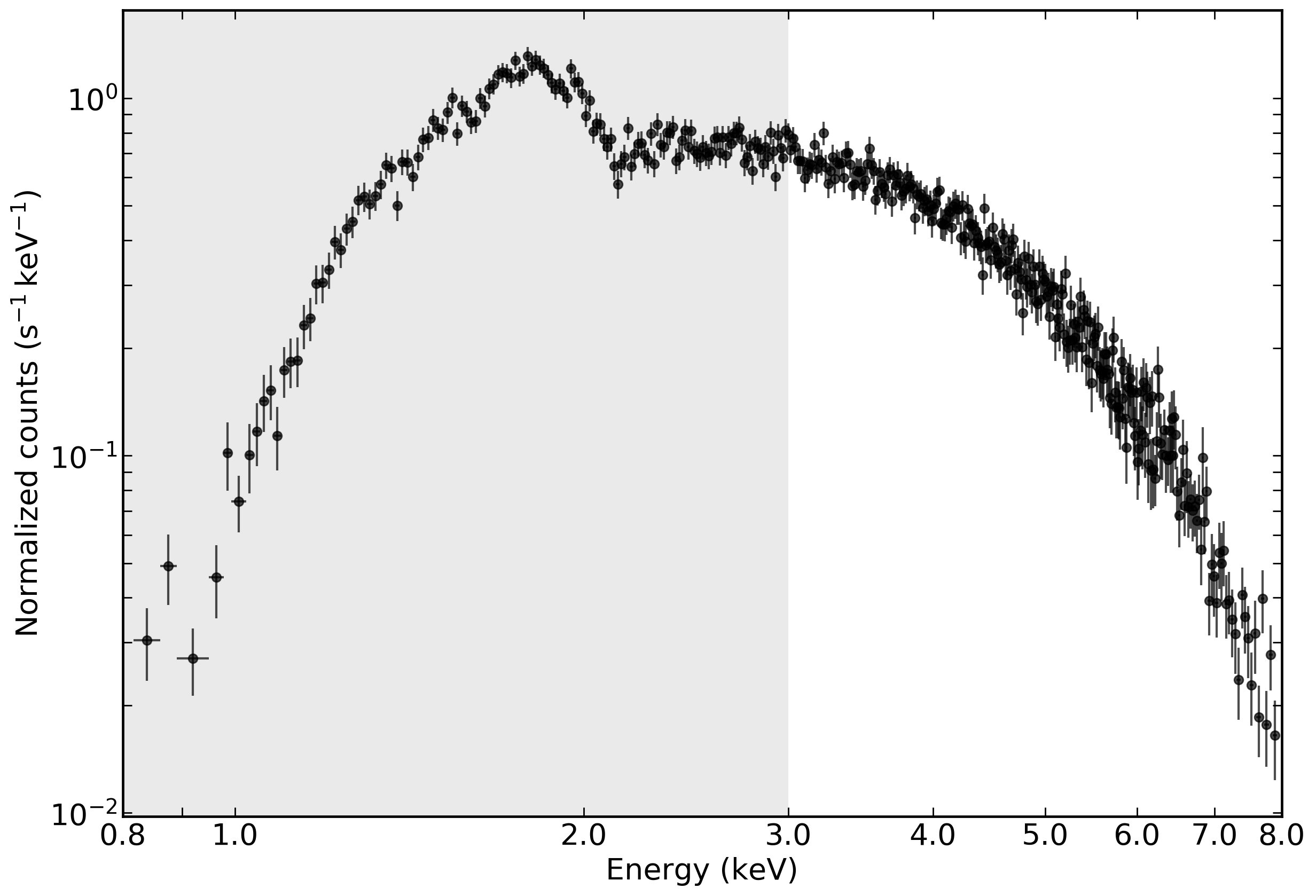
Figure 7: Spectrum of the Chandra ACIS detector in the 0.8–8 keV range. Only the spectra from the longest observation (ObsID 1433) is shown. The grey and white shaded regions show the different fitting energy bands: 0.8–3 keV, 3–8 keV.

The NuSTAR data were fit in the 3.0–8.0 keV, 8–20 keV, and 20–45 keV energy bands. While NuSTAR operates in the 3–79 keV range, the spectral fitting for this source was restricted to the 3–45 keV range as the background dominates above 45 keV. In addition, the spectra from FPMA and FPMB were fit separately as we noticed a consistent difference in the fit parameters when performing fits for each spectra independently. Specifically, we saw that the photon index $\Gamma$ was higher for FPMA spectra compared to FPMB spectra and that the unabsorbed flux was consistently higher for FPMB spectra compared to FPMA spectra. This discrepancy between the FPMA and FPMB spectra is described in Appendix A. This issue is unrelated to the discrepancy due to a thermal blanket tear for the FPMA detector causing an excess in low-energy photons (Madsen et al., 2020) as the NuSTAR team believes the tear began in 2017, and all the observations analyzed in this study are from 2012 and 2013 (Table 4). The spectra from the longest observation are shown in Figure 8.

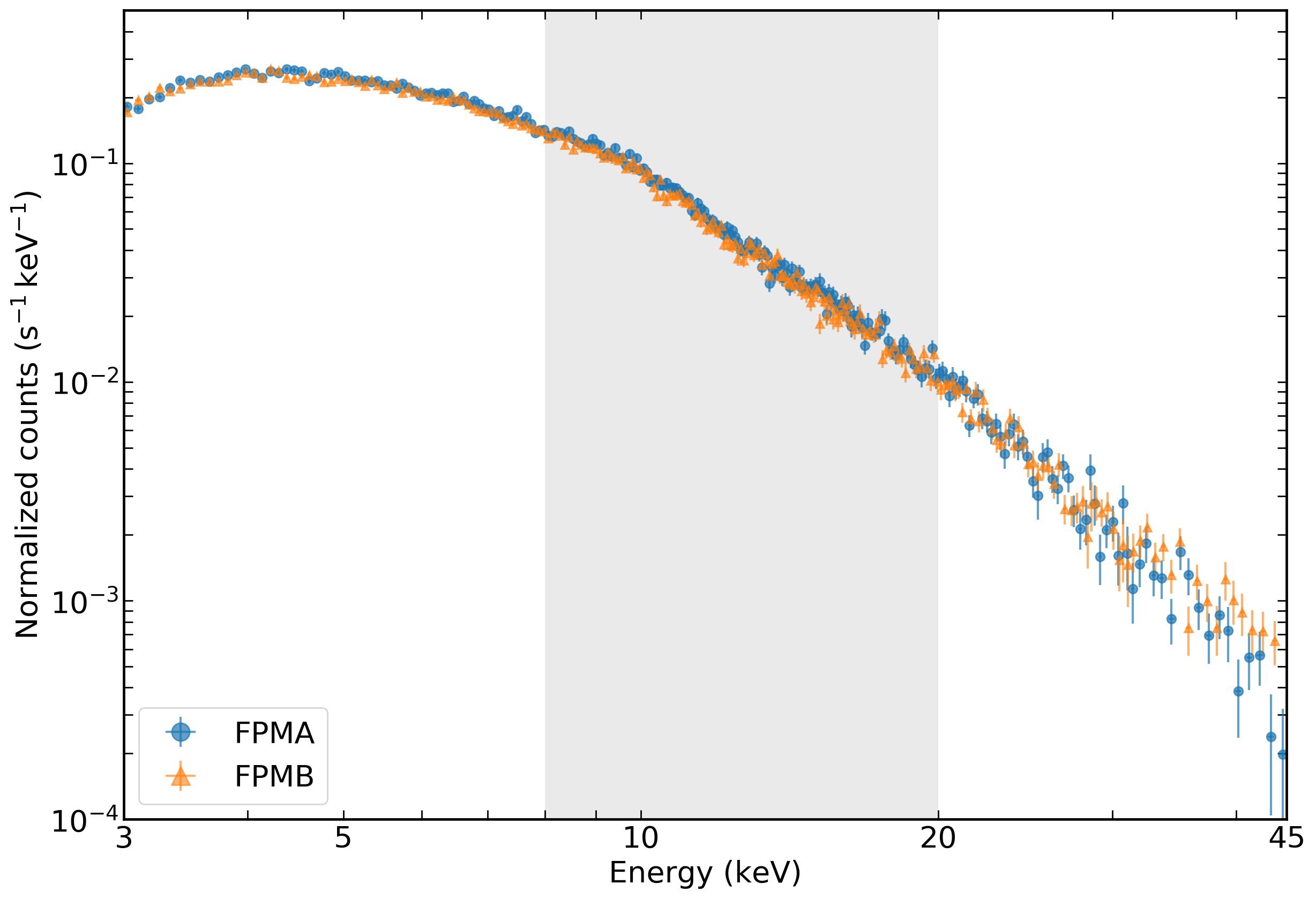
Figure 8: Wide-band spectra of the NuSTAR FPMA (blue) and FPMB (orange) detectors in the 3–45 keV range. Only the spectra from the longest observation (ObsID 10002014005) are shown to prevent overcrowding the figure. The alternating white-grey bands show the different fitting energy bands: 3–8 keV, 8–20 keV (grey), 20–45 keV.

The data recorded by Hitomi spans the combined energy range of the Chandra and NuSTAR observations. Hence the Hitomi data were fit over all specified energy bands. Given that the full energy range of Hitomi is spread over two different type of detectors, we report on the results of each energy band for the respective detector sensitive to those energies. (see Tables 6, 7, 8, 9). The observed spectra are shown in Figure 9, where the detector spectrum relevant for each energy band is indicated.

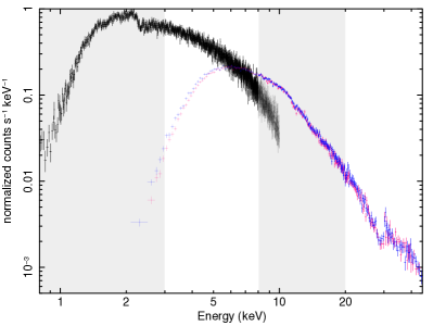
Figure 9: Wide-band spectra of the Hitomi SXI (black) and HXI detectors (HXI1 in blue and HXI2 in magenta) in the $0.8-45$ keV energy range. The different fitting energy bands are indicated by the alternating grey bands. Data that is not fitted in a given energy band is made transparent.

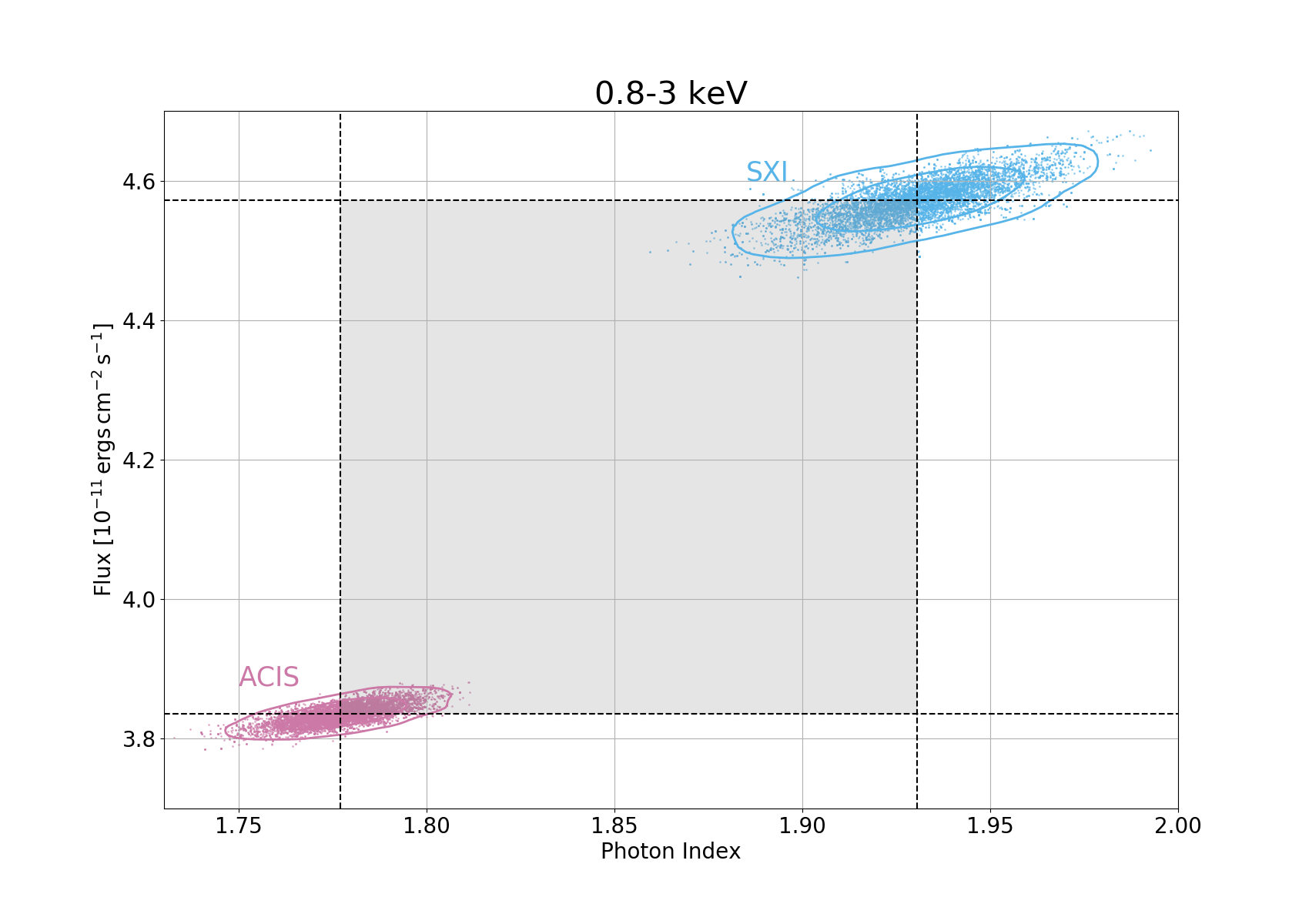
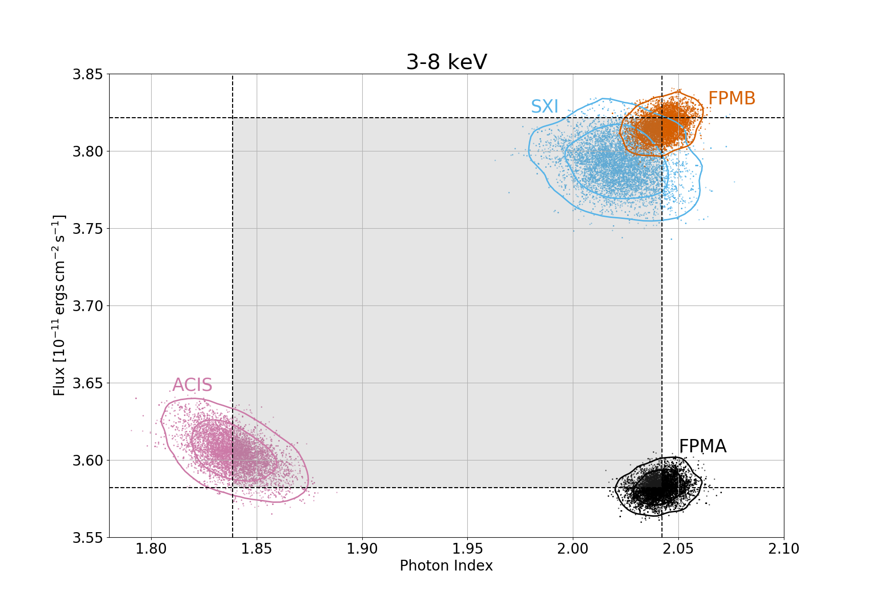
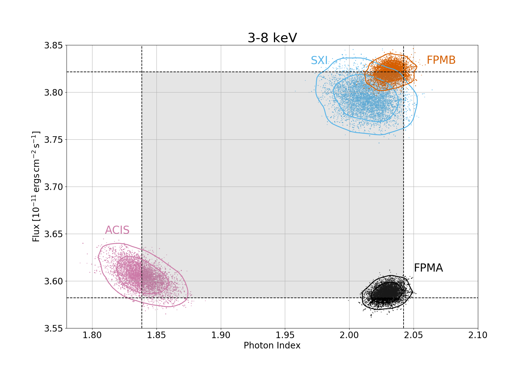
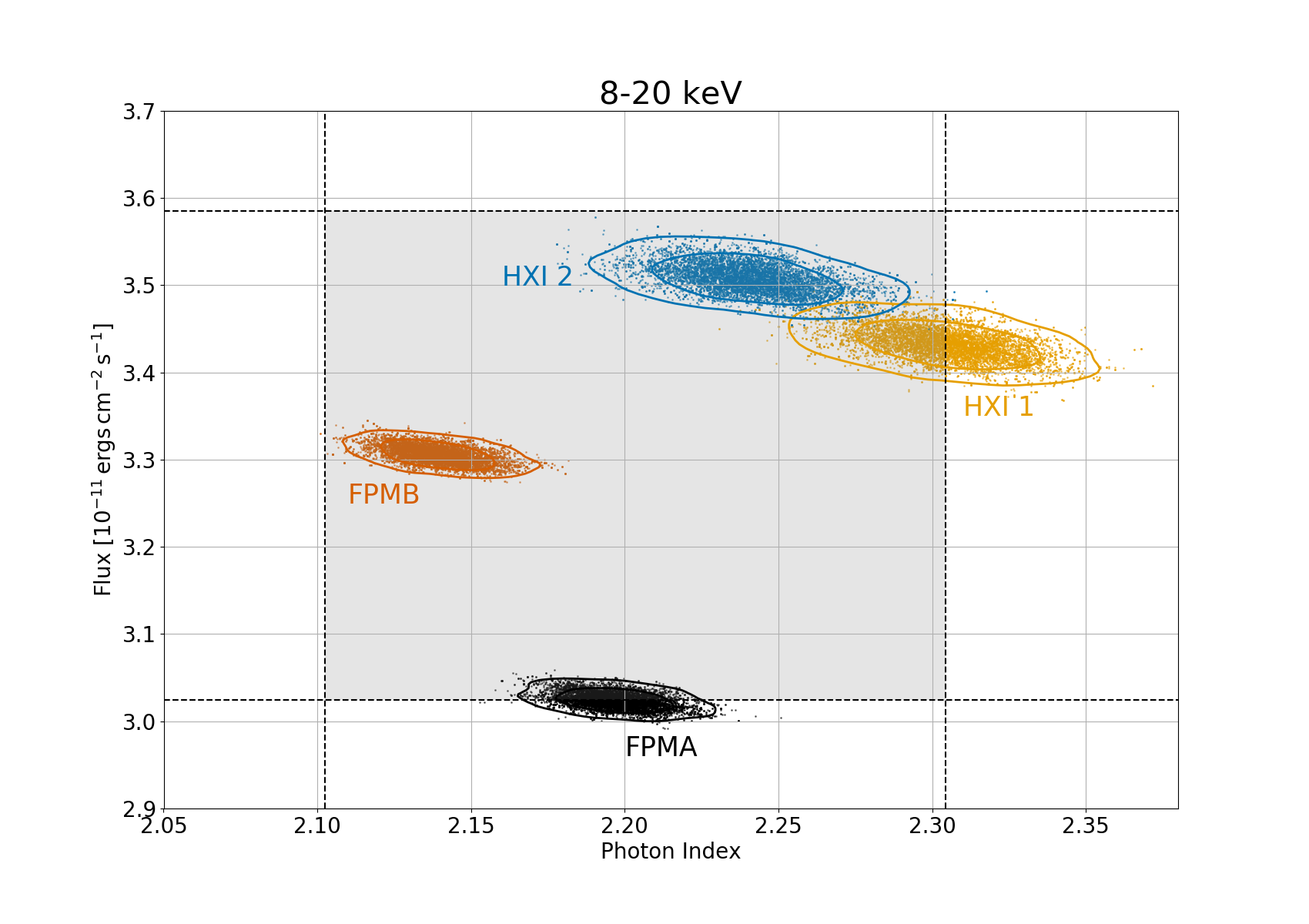
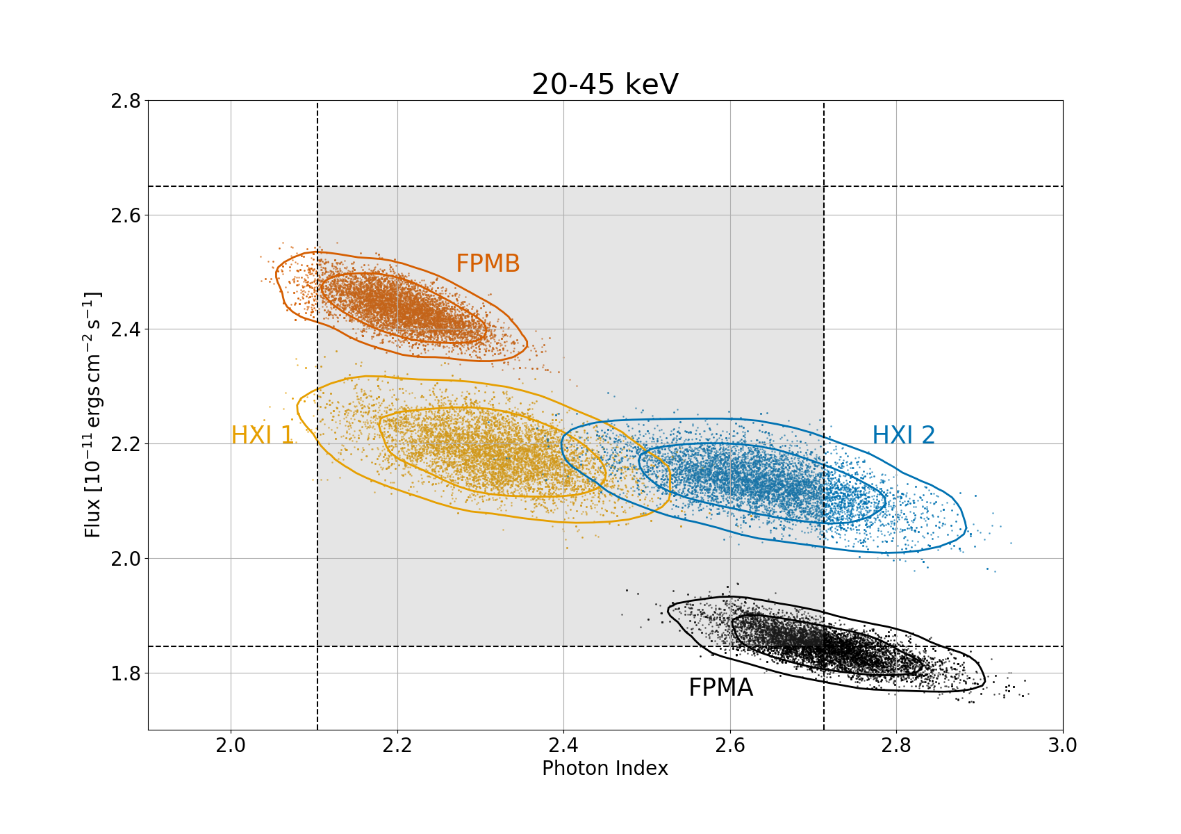
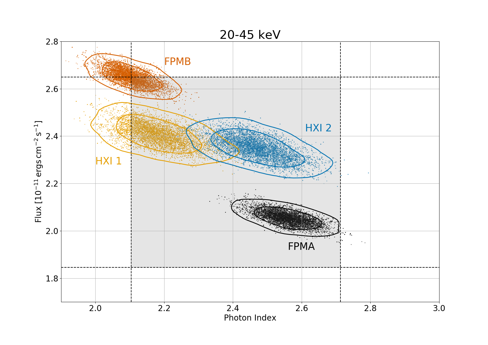
Figure 10: Scatter plots of the MCMC samples (Photon index $\Gamma$ and unabsorbed flux $F$). The contours are drawn at the regions containing 68% and 95% of the samples. Each row shows a different energy range in increasing order from top to bottom. The left column is for the model with the pulsar black-body component and the right column is for the model without the black-body component. The shaded areas are consistent within a row and their role is explained in. 4.2.

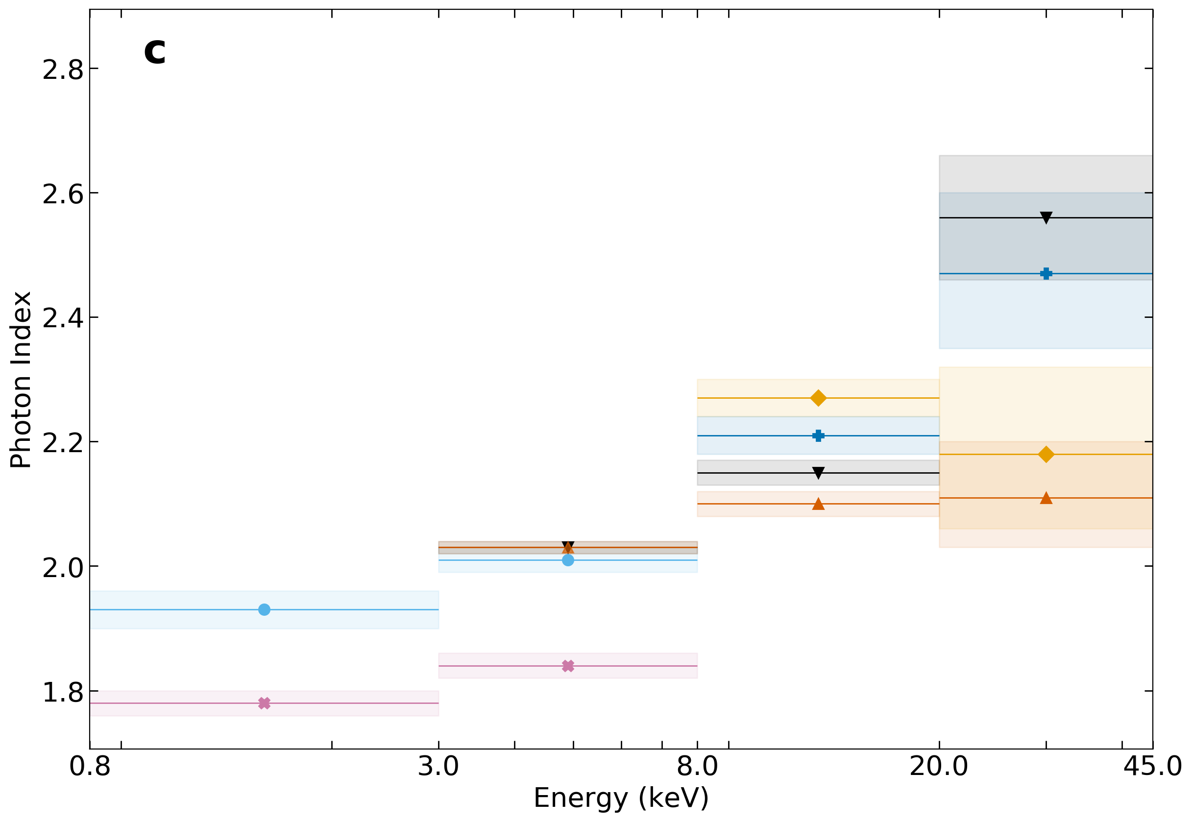
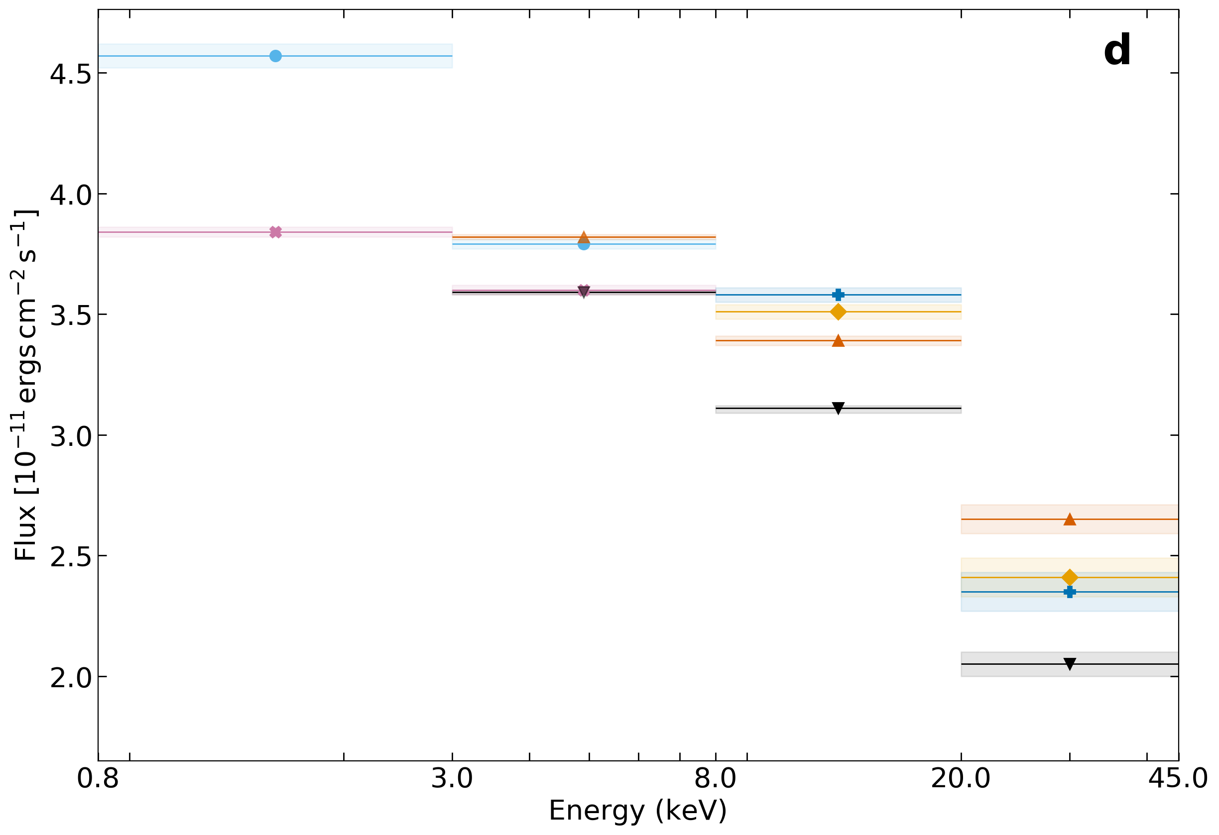
Figure 11: Plots showing the PWN fit parameter values for the detectors in each energy range. Plots a, b are the photon indices and flux values for the model with the black-body component, and plots c, d are the photon indices and flux values for the model without the black-body component. The shaded regions indicate the 90% confidence intervals consistent with those given in the tables.

Table 6: PWN Photon index $\Gamma$ per energy range for each detector when fitting the model with a pulsar black-body component

Energy Range [keV]	Chandra	Hitomi SXI	Hitomi HXI 1	Hitomi HXI 2	NuSTAR FPMA	NuSTAR FPMB
0.8 – 3.0	$1.78\begin{subarray}{c}+0.02\\ -0.02\end{subarray}$	$1.93\begin{subarray}{c}+0.03\\ -0.03\end{subarray}$	–	–	–	–
3–8	$1.84\begin{subarray}{c}+0.02\\ -0.02\end{subarray}$	$2.02\begin{subarray}{c}+0.02\\ -0.02\end{subarray}$	–	–	$2.04\begin{subarray}{c}+0.01\\ -0.01\end{subarray}$	$2.04\begin{subarray}{c}+0.01\\ -0.01\end{subarray}$
8–20	–	–	$2.31\begin{subarray}{c}+0.03\\ -0.03\end{subarray}$	$2.24\begin{subarray}{c}+0.03\\ -0.03\end{subarray}$	$2.20\begin{subarray}{c}+0.02\\ -0.02\end{subarray}$	$2.14\begin{subarray}{c}+0.02\\ -0.02\end{subarray}$
20–45	–	–	$2.32\begin{subarray}{c}+0.13\\ -0.14\end{subarray}$	$2.64\begin{subarray}{c}+0.15\\ -0.15\end{subarray}$	$2.71\begin{subarray}{c}+0.13\\ -0.11\end{subarray}$	$2.21\begin{subarray}{c}+0.09\\ -0.09\end{subarray}$

Table 7: PWN Photon index $\Gamma$ per energy range for each detector when fitting the model without a pulsar black-body component

Energy Range [keV]	Chandra	Hitomi SXI	Hitomi HXI 1	Hitomi HXI 2	NuSTAR FPMA	NuSTAR FPMB
0.8–3.0	$1.78\begin{subarray}{c}+0.02\\ -0.02\end{subarray}$	$1.93\begin{subarray}{c}+0.03\\ -0.03\end{subarray}$	–	–	–	–
3–8	$1.84\begin{subarray}{c}+0.02\\ -0.02\end{subarray}$	$2.01\begin{subarray}{c}+0.02\\ -0.02\end{subarray}$	–	–	$2.03\begin{subarray}{c}+0.01\\ -0.01\end{subarray}$	$2.03\begin{subarray}{c}+0.01\\ -0.01\end{subarray}$
8–20		–	$2.27\begin{subarray}{c}+0.03\\ -0.03\end{subarray}$	$2.21\begin{subarray}{c}+0.03\\ -0.03\end{subarray}$	$2.15\begin{subarray}{c}+0.02\\ -0.02\end{subarray}$	$2.10\begin{subarray}{c}+0.02\\ -0.02\end{subarray}$
20–45		–	$2.18\begin{subarray}{c}+0.14\\ -0.12\end{subarray}$	$2.47\begin{subarray}{c}+0.13\\ -0.12\end{subarray}$	$2.56\begin{subarray}{c}+0.10\\ -0.10\end{subarray}$	$2.11\begin{subarray}{c}+0.09\\ -0.08\end{subarray}$

Table 8: PWN unabsorbed flux per energy range for each detector when fitting the model with a pulsar black-body component

Energy Range [keV]	Chandra	Hitomi SXI	Hitomi HXI 1	Hitomi HXI 2	NuSTAR FPMA	NuSTAR FPMB
0.8–3.0	$3.84\begin{subarray}{c}+0.02\\ -0.02\end{subarray}$	$4.57\begin{subarray}{c}+0.05\\ -0.05\end{subarray}$	–	–	–	–
3–8	$3.60\begin{subarray}{c}+0.02\\ -0.02\end{subarray}$	$3.79\begin{subarray}{c}+0.02\\ -0.02\end{subarray}$	–	–	$3.58\begin{subarray}{c}+0.01\\ -0.01\end{subarray}$	$3.82\begin{subarray}{c}+0.01\\ -0.01\end{subarray}$
8–20	–	–	$3.43\begin{subarray}{c}+0.03\\ -0.03\end{subarray}$	$3.51\begin{subarray}{c}+0.03\\ -0.03\end{subarray}$	$3.02\begin{subarray}{c}+0.02\\ -0.01\end{subarray}$	$3.31\begin{subarray}{c}+0.02\\ -0.02\end{subarray}$
20–45	–	–	$2.19\begin{subarray}{c}+0.08\\ -0.07\end{subarray}$	$2.13\begin{subarray}{c}+0.07\\ -0.07\end{subarray}$	$1.84\begin{subarray}{c}+0.05\\ -0.05\end{subarray}$	$2.43\begin{subarray}{c}+0.06\\ -0.06\end{subarray}$

Table 9: PWN unabsorbed flux per energy range for each detector when fitting the model without a pulsar black-body component

Energy Range [keV]	Chandra	Hitomi SXI	Hitomi HXI 1	Hitomi HXI 2	NuSTAR FPMA	NuSTAR FPMB
0.8–3.0	$3.84\begin{subarray}{c}+0.02\\ -0.02\end{subarray}$	$4.57\begin{subarray}{c}+0.05\\ -0.05\end{subarray}$	–	–	–	–
3–8	$3.60\begin{subarray}{c}+0.02\\ -0.02\end{subarray}$	$3.79\begin{subarray}{c}+0.03\\ -0.02\end{subarray}$	–	–	$3.59\begin{subarray}{c}+0.01\\ -0.01\end{subarray}$	$3.82\begin{subarray}{c}+0.01\\ -0.01\end{subarray}$
8–20	–	–	$3.51\begin{subarray}{c}+0.03\\ -0.03\end{subarray}$	$3.58\begin{subarray}{c}+0.03\\ -0.03\end{subarray}$	$3.11\begin{subarray}{c}+0.01\\ -0.02\end{subarray}$	$3.39\begin{subarray}{c}+0.02\\ -0.02\end{subarray}$
20–45	–	–	$2.41\begin{subarray}{c}+0.08\\ -0.08\end{subarray}$	$2.35\begin{subarray}{c}+0.08\\ -0.08\end{subarray}$	$2.05\begin{subarray}{c}+0.05\\ -0.05\end{subarray}$	$2.65\begin{subarray}{c}+0.06\\ -0.06\end{subarray}$

3.3 Results

As mentioned in 3.1, we fit two different models: one model incorporating a pulsar black-body component and another model without a pulsar black-body component, to the X-ray spectra. We show the results of the fits for the photon index and normalization (i.e., unabsorbed flux) parameters for the PWN spectra in Figure 10; Tables 6, 7, 8, 9; and Figure 11. Figure 10 is a collection of scatter plots showing the MCMC samples. The contours indicate regions containing 68% and 95% of the samples, respectively. The results are also tabulated in Tables 6, 7, 8, 9. The uncertainties in the tables are the one-dimensional 90% confidence intervals. Figure 11 shows the two fit parameters separately with energy on the x-axis to highlight differences between energy bands.

As shown in Table 5, the photon index for the pulsar component is $\Gamma=1.35$ when including the black-body, while $\Gamma=1.54$ when excluding the black-body component. This increase of $\sim 0.2$ in $\Gamma$ when excluding the black-body model assumes a softer spectrum for the pulsar component. As a softer spectrum for the pulsar component implies that the pulsar’s emission is more concentrated at lower energies and does not extend to higher energies, a larger fraction of the overall emission at higher energies is attributed to the PWN. This effect results in a harder spectrum for the PWN (i.e., smaller $\Gamma$). This difference in $\Gamma$ for the PWN component between the two models is larger for higher energies.

While the photon index $\Gamma$ from different detectors in the same energy band do not necessarily agree (Figure 10), overall we see a general spectral softening (i.e., increase in $\Gamma$) over the four energy bands (Figure 11). An exception to this trend is Hitomi’s HXI 1 detector when fitting with the model that does not contains the pulsar black-body component (Table 7) in the 20–45 keV band. However, while the best-fit photon index changes from $\Gamma=2.27$ in the 8–20 keV band to $\Gamma=2.18$ in the 20–45 keV band, the uncertainty in the 20–45 keV band is large enough to make a softening plausible.

Regarding the normalization (i.e., unabsorbed flux) parameter, while the values of the normalization parameter decrease for each detector as we go from lower energy bands to higher energy bands, similar to the photon index within the same energy band the values from different detectors disagree.

Next, we discuss how we incorporate the uncertainties in the fit parameters, due to the disagreement between detectors and the choice to include/exclude the pulsar black-body component, into our PWN modelling.

4 Discussion

Here we discuss the results of modelling the PWN while taking into consideration the above IR and X-ray analysis. In §4.1 we discuss the potential origin of the observed IR emission. We then use this information and our updated X-ray analysis to determine the observed properties which should be reproduced by a physical model for the evolution of a PWN inside a SNR. In §4.2, we describe such an evolutionary model and the method by which we identified the combination of input parameters that best reproduces the observed properties of this system. We further discuss the implications of the derived values for the model parameters in §4.2, and use them to constrain structures in the surrounding ISM needed to reproduce the morphology of the surrounding SNR shell in §4.3.

4.1 Infrared Emission

As mentioned in §1, previous attempts to model the emission of this PWN were unable to simultaneously reproduce the obsreved IR and X-ray spectrum assuming both were synchrotron emission from the PWN (e.g., Torres et al. 2014; Hitomi Collaboration et al. 2018). While the power-law spectrum for the X-ray emission derived in our analysis (§3.3) strongly suggests this is correct, below we evaluate if the IR emission is also synchrotron radiation from high-energy leptons in the PWN.

The total IR flux densities of the PWN region in  are listed in Table 2 and plotted in Figure 12. Figure 2 shows the [O I] 63.2 $\mu$m and [C II] 157.7 $\mu$m line maps in left and middle panels, as well as the MIPS 24 µm of the PWN region in the right panel for comparison. These lines contribute to the emission seen in the Herschel PACS 70 and 160 µm images shown in Figure 3. Since the emission at 24 µm has a similar filamentary morphology as the [O I] 63.2 $\mu$m map, it is not unreasonable to assume that a significant part of the emission seen at 24 µm arises from O IV or Fe II ejecta lines that fall in the wavelength range of the MIPS bandpass.

As a result, it is likely that a significant fraction of the IR emission detected from this source is produced by dust and gas that resides in the ejecta filaments. In order to use the IR properties of this sources to study the innermost dust and gas inside the SNR, it is first necessary to quantify the contribution from the PWN. Often this is done by simply extrapolating a power-law fit to the spectrum at higher (typically X-ray) or lower (GHz radio) frequencies (e.g., Koo et al. 2016). However, the modeling described below in §4.2 potentially provides a more accurate way of estimating the synchrotron IR emission from the PWN.

4.2 Modeling of PWN

As discussed in §1, the properties of a PWN inside a SNR provide invaluable information on the progenitor star and supernova explosion, the birth properties of the neutron star, and the content of its pulsar wind. Currently, one of the best methods of obtaining these properties is to use a (time-dependent) model for the evolution of a PWN in a SNR to reproduce the dynamical and broadband spectral energy distribution (SED) of a particular system (see recent reviews by Gelfand 2017 and Slane 2017 as well as references therein). Here, we use the evolutionary model described by Gelfand et al. (2009) to reproduce the properties listed in Table 10, as we have previously done for the PWNe in G54.1+0.3 (Gelfand et al., 2015), HESS J1640$-$465 (Gotthelf et al., 2014), and Kes 75 (Gelfand et al., 2013).

Table 10: Observed properties of  used in the modeling of this source

Property	Observed	“Best Fit” Values		Citation
$\cdots$	$\cdots$	Variable $p$	$p\equiv 1.85690$	$\cdots$
PSR J1833$-$1034
Current spin-down luminosity $\dot{E}$	$3.37\times 10^{37}~{}\frac{\rm erg}{\rm s}$	$\cdots$	$\cdots$	Camilo et al. (2006)
Current characteristic age $t_{\rm ch}$	4850 years	$\cdots$	$\cdots$	Camilo et al. (2006)
Pulsar Wind Nebula
Angular radius $\theta_{\rm pwn}$	$40\arcsec\pm 4\arcsec$	$42\farcs 6$	$40\farcs 5$	Matheson & Safi-Harb (2010)
Angular expansion rate $\dot{\theta}_{\rm pwn}$	$(0.11\pm 0.02)\frac{\%}{\rm year}$	$0.07\frac{\%}{\rm year}$	$0.07\frac{\%}{\rm year}$	Bietenholz & Bartel (2008)
327 MHz Flux Density	$7.3\pm 0.7$ Jy	5.8 Jy	4.9 Jy	Bietenholz et al. (2011)
1.43 GHz Flux Density	$7.0\pm 0.4$ Jy	7.2 Jy	6.4 Jy	Bietenholz et al. (2011)
4.8 GHz Flux Density	$6.5\pm 0.4$ Jy	7.5 Jy	6.9 Jy	Sun et al. (2011)
4.49 – 7.85 GHz Spectral Index	$-0.12\pm 0.03$	$-0.06\pm 0.01$	$-0.03\pm 0.01$	Bhatnagar et al. (2011)
70 GHz Flux Density	$4.3\pm 0.6$ Jy	3.7 Jy	3.7 Jy	Planck Collaboration et al. (2016)
84.2 GHz Flux Density	$3.9\pm 0.7$ Jy	3.5 Jy	3.5 Jy	Salter et al. (1989b)
90.7 GHz Flux Density	$3.8\pm 0.4$ Jy	3.2 Jy	3.3 Jy	Salter et al. (1989a)
94 GHz Flux Density	$3.5\pm 0.4$ Jy	3.2 Jy	3.3 Jy	Bock et al. (2001)
100 GHz Flux Density	$2.7\pm 0.5$ Jy	3.0 Jy	3.1 Jy	Planck Collaboration et al. (2016)
141.9 GHz Flux Density	$2.5\pm 1.2$ Jy	2.4 Jy	2.5 Jy	Salter et al. (1989a)
143 GHz Flux Density	$3.0\pm 0.4$ Jy	2.4 Jy	2.5 Jy	Planck Collaboration et al. (2016)
$0.8-3.0$ keV Unabsorbed Flux	$(3.84_{-0.02}-4.57^{+0.05})\times 10^{-11}~{}\frac{\rm ergs}{\rm cm^{2}~{}s}$	$4.46\times 10^{-11}~{}\frac{\rm ergs}{\rm cm^{2}~{}s}$	$4.46\times 10^{-11}~{}\frac{\rm ergs}{\rm cm^{2}~{}s}$	Tables 8 & 9
$0.8-3.0$ keV Photon Index	$1.78_{-0.02}-1.93^{+0.03}$	$1.84\pm 0.01$	$1.84\pm 0.01$	Tables 6 & 7
$3.0-8.0$ keV Unabsorbed Flux	$(3.58_{-0.01}-3.82^{+0.01})\times 10^{-11}~{}\frac{\rm ergs}{\rm cm^{2}~{}s}$	$3.82\times 10^{-11}~{}\frac{\rm ergs}{\rm cm^{2}~{}s}$	$3.82\times 10^{-11}~{}\frac{\rm ergs}{\rm cm^{2}~{}s}$	Tables 8 & 9
$3.0-8.0$ keV Photon Index	$1.84_{-0.02}-2.04^{+0.01}$	$2.01\pm 0.02$	$2.00\pm 0.02$	Tables 6 & 7
$8.0-20.0$ keV Unabsorbed Flux	$(3.02_{-0.02}-3.58^{+0.04})\times 10^{-11}~{}\frac{\rm ergs}{\rm cm^{2}~{}s}$	$3.02\times 10^{-11}~{}\frac{\rm ergs}{\rm cm^{2}~{}s}$	$3.04\times 10^{-11}~{}\frac{\rm ergs}{\rm cm^{2}~{}s}$	Tables 8 & 9
$8.0-20.0$ keV Photon Index	$2.10_{-0.02}-2.31^{+0.03}$	$2.19\pm 0.02$	$2.17\pm 0.02$	Tables 6 & 7
$20.0-45.0$ keV Unabsorbed Flux	$(1.84_{-0.05}-2.65^{+0.06})\times 10^{-11}~{}\frac{\rm ergs}{\rm cm^{2}~{}s}$	$2.05\times 10^{-11}~{}\frac{\rm ergs}{\rm cm^{2}~{}s}$	$2.11\times 10^{-11}~{}\frac{\rm ergs}{\rm cm^{2}~{}s}$	Tables 8 & 9
$20.0-45.0$ keV Photon Index	$2.10_{-0.08}-2.71^{+0.13}$	$2.65\pm 0.03$	$2.61\pm 0.03$	Tables 6 & 7
$10-20$ GeV Photon Flux	$8.6_{-2.2}^{+2.5}\times 10^{-11}~{}\frac{\rm photons}{\rm cm^{2}~{}s}$	$6.36\times 10^{-11}~{}\frac{\rm photons}{\rm cm^{2}~{}s}$	$6.15\times 10^{-11}~{}\frac{\rm photons}{\rm cm^{2}~{}s}$	Ajello et al. (2017)
$20-50$ GeV Photon Flux	$1.85_{-0.93}^{+1.23}\times 10^{-11}~{}\frac{\rm photons}{\rm cm^{2}~{}s}$	$3.05\times 10^{-11}~{}\frac{\rm photons}{\rm cm^{2}~{}s}$	$2.94\times 10^{-11}~{}\frac{\rm photons}{\rm cm^{2}~{}s}$	Ajello et al. (2017)
$150-500$ GeV Photon Flux	$<6.31\times 10^{-12}~{}\frac{\rm photons}{\rm cm^{2}~{}s}$ (3$\sigma$)	$2.75\times 10^{-12}~{}\frac{\rm photons}{\rm cm^{2}~{}s}$	$2.61\times 10^{-12}~{}\frac{\rm photons}{\rm cm^{2}~{}s}$	Ajello et al. (2017)
$0.5-1.2$ TeV Photon Flux	$<5.34\times 10^{-12}~{}\frac{\rm photons}{\rm cm^{2}~{}s}$ (3$\sigma$)	$6.59\times 10^{-13}~{}\frac{\rm photons}{\rm cm^{2}~{}s}$	$6.15\times 10^{-13}~{}\frac{\rm photons}{\rm cm^{2}~{}s}$	Ajello et al. (2017)
$1-10$ TeV Flux	$(1.29\pm 0.25)\times 10^{-12}~{}\frac{\rm ergs}{\rm cm^{2}~{}s}$	$1.21\times 10^{-12}~{}\frac{\rm ergs}{\rm cm^{2}~{}s}$	$1.10\times 10^{-12}~{}\frac{\rm ergs}{\rm cm^{2}~{}s}$	H. E. S. S. Collaboration et al. (2018)
$1-10$ TeV Photon Index	$2.4\pm 0.2$	$2.25\pm 0.01$	$2.27\pm 0.01$	H. E. S. S. Collaboration et al. (2018)
Supernova Remnant
Angular radius $\theta_{\rm snr}$	$2\farcm 44\pm 0\farcm 24$	$2\farcm 55$	$2\farcm 56$	Guest et al. (2019)
$v_{\rm ej}(R_{\rm pwn})$	$350-1000~{}\frac{\rm km}{\rm s}$	$525~{}\frac{\rm km}{\rm s}$	$525~{}\frac{\rm km}{\rm s}$	§2.1
Distance	4.4 kpc	$\cdots$	$\cdots$	Ranasinghe & Leahy (2018)

The input parameters to this model are listed in Table 11. As in the past analyses listed above, we make the following assumptions:

1. Assume that the density profile of the unshocked SN ejecta consists of a uniform density $(\rho\propto r^{0})$ core surrounded by a $\rho\propto r^{-9}$ envelope. While this assumption is common in this field (see Gelfand 2017 for a recent review), as discussed by Chevalier (2005) different supernova progenitors will likely have different ejecta density profiles.

2. Assume that the supernova ejecta with mass $M_{\rm ej}$ and initial kinetic energy $E_{\rm sn}$ is expanding into a medium with uniform density $n_{\rm ism}$. As discussed in §4.3, the X-ray morphology of the SNR shell strongly suggests a density enhancement North of the explosion site. However, as this enhancement has only impacted a small fraction of the shell – not affecting the average SNR radius $\theta_{\rm snr}$ used in our modeling – nor caused the SN reverse shock to collide with any part of the PWN, this has a minimal effect on the results of our modeling.

3. Calculate the age $t_{\rm age}$ and initial spin-down luminosity $\dot{E}_{0}$ of associated PSR J1833$-$1034 for a particular (assumed constant) pulsar braking index $p$ and spin-down timescale $\tau_{\rm sd}$ using the characteristic age $t_{\rm ch}$ and current spin-down luminosity $\dot{E}$ (given in Table 10) inferred from the measured period $P$ and period-derivative $\dot{P}$ of the PSR (e.g., Gelfand et al. 2015):

   $$t_{\rm age} = \frac{2t_{\rm ch}}{p-1}-\tau_{\rm sd}$$ (1)

   $$\dot{E}_{0} = \dot{E}\left(1+\frac{t_{\rm age}}{\tau_{\rm sd}}\right)^{+\frac{p+1}{p-1}}$$ (2)

4. Assume the entire spin-down luminosity $\dot{E}$ is injected into the PWN as either magnetic fields $\dot{E}_{\rm B}$ or the kinetic energy $\dot{E}_{\rm p}$ of relativistic leptons ($e^{\pm}$), such that:

   $$\dot{E}_{\rm B}(t) = \eta_{\rm B}\dot{E}(t)=\eta_{\rm B}\dot{E}_{0}\left(1+\frac{t}{\tau_{\rm sd}}\right)^{-\frac{p+1}{p-1}}$$ (3)

   $$\dot{E}_{\rm p}(t) = (1-\eta_{\rm B})\dot{E}(t)=(1-\eta_{\rm B})\dot{E}_{0}\left(1+\frac{t}{\tau_{\rm sd}}\right)^{-\frac{p+1}{p-1}}$$ (4)

   where $\eta_{\rm B}$ is constant with time. While the pulsed $\gamma$-ray luminosity of some pulsars can be a significant fraction of $\dot{E}$, the observed pulsed $\gamma$-ray luminosity of PSR J1833$-$1034 is $\approx 0.005\dot{E}$ (Abdo et al., 2013).

5. Assume that the spectrum of particles injected into the PWN is well-described by a broken power-law of the form:

   $$\frac{d\dot{N}}{dE} = \left\{\begin{array}[]{cc}\dot{N}_{\rm break}\left(\frac{E}{E_{\rm break}}\right)^{-p_{1}}&E_{\rm min}<E<E_{\rm break}\\ \dot{N}_{\rm break}\left(\frac{E}{E_{\rm break}}\right)^{-p_{2}}&E_{\rm break}<E<E_{\rm max}\\ \end{array}\right.$$ (7)

   where the five free parameters ($E_{\rm min}$, $E_{\rm break}$, $E_{\rm max}$, $p_{1}$, and $p_{2}$) in Equation 7 are assumed to be constant with time and the normalization $\dot{N}_{\rm break}$ is calculated by requiring that:

   $$\dot{E}_{\rm p} = \int\limits_{E_{\rm min}}^{E_{\rm max}}E\frac{d\dot{N}}{dE}dE$$ (8)

   at all times $t$.

6. Assume that only radiative losses suffered by particles trapped within the PWN are the result of synchrotron and inverse Compton (IC) emission. When calculating synchrotron losses, we assume the PWN’s magnetic field has a uniform strength $B_{\rm pwn}(t)$ (whose evolution is calculated using the procedure described by Gelfand et al. 2009) and that the particle pitch angles (i.e., the angle between their velocity $\vec{v}$ and local magnetic field $\vec{B}$) is randomly distributed. For IC emission, we consider particles scattering photons emitted by the Cosmic Microwave Background (temperature $T_{\rm cmb}=2.7255~{}{\rm K}$; Fixsen 2009) as well as an additional background field which has a blackbody spectrum with temperature $T_{\rm ic}$ and normalization $K_{\rm ic}$, such that this photon field has an energy density:

   $$u_{\rm ic} = K_{\rm ic}a_{\rm bb}T_{\rm ic}^{4},$$ (9)

   where $a_{\rm bb}\approx 7.5657\times 10^{-15}~{}\frac{\rm ergs}{\rm cm^{3}K^{4}}$. We do not consider Synchrotron Self-Compton (SSC) emission, since previous theoretical work have found that SSC emission significantly contributes to the total IC emission only at extremely early times (e.g., Gelfand et al. 2009; Martín et al. 2012).

To convert the physical quantities predicted by our model to the observed properties of this system, we assume a distance $d\equiv 4.4~{}{\rm kpc}$ – the central value derived from a recent study of its Hi emission ($d=4.4\pm 0.2$ kpc; Ranasinghe & Leahy 2018).

Table 11: PWN model parameters which best reproduces the properties of

Model Parameter	Variable $p$	$p\equiv 1.85690$
Supernova Explosion Energy $E_{\rm sn}$	$1.2\times 10^{50}~{}{\rm ergs}$	$1.2\times 10^{50}~{}{\rm ergs}$
Supernova Ejecta Mass $M_{\rm ej}$	11.32 M⊙	11.33 M⊙
ISM Density $n_{\rm ism}$	0.2 cm-3	0.2 cm-3
Pulsar Braking Index $p$	3.126	$\equiv 1.85690$
Pulsar Spindown Timescale $\tau_{\rm sd}$	2900 years	9600 years
Wind Magnetization $\eta_{\rm B}$	$3.2\times 10^{-3}$	$3.5\times 10^{-3}$
Minimum Energy of Injected Leptons $E_{\rm min}$	12.5 GeV	12.5 GeV
Break Energy of Injected Leptons $E_{\rm break}$	1.0 TeV	1.0 TeV
Maximum Energy of Injected Leptons $E_{\rm max}$	0.26 PeV	0.18 PeV
Low-Energy Particle Index $p_{1}$	2.86	2.86
High-Energy Particle Index $p_{2}$	2.51	2.51
Temperature of External Photon Field $T_{\rm ic}$	1700 K	1700 K
Normalization of External Photon Field $K_{\rm ic}$	$3.5\times 10^{-10}$	$3.8\times 10^{-10}$
$\chi^{2}$ / degrees of freedom	30 / 16	37 / 17

We used a Metropolis MCMC algorithm (Metropolis 1985; see §3.2 of Gelfand et al. (2015) for a detailed description) to identify the combination of the 13 model input parameters $\Theta$ listed in Table 11 which best reproduce the 29 observed properties ${\mathcal{D}}$ of  listed in Table 10. This is accomplished by the maximum likelihood estimation method, in which we find the combination $\Theta$ whose predicted values of the observed properties ${\mathcal{M}}$ maximizes the likelihood ${\mathcal{L}}({\mathcal{D}}|\Theta)$:

$${\mathcal{L}} \equiv \prod\limits_{i=1}^{29}{\mathcal{L}}({\mathcal{D}}_{i}|\Theta)$$ (10)

$$\ln{\mathcal{L}} = \sum\limits_{i=1}^{29}\ln{\mathcal{L}}({\mathcal{D}}_{i}|\Theta)$$ (11)

As listed in Table 10, there are three types of observed quantities ${\mathcal{D}}_{i}$, those:

1. whose measured error $\sigma_{i}$ is Gaussian in nature (indicated by $\pm$ in Table 10),

2. constrained to be below some value ${\mathcal{D}}_{i}<{\mathcal{D}}_{i}^{\rm up}$ (indicated by $<$ in Table 10), and

3. whose true value is believed to lie within a range ${\mathcal{D}}_{i}^{\rm lo}<{\mathcal{D}}_{i}<{\mathcal{D}}_{i}^{\rm hi}$.

The likelihood ${\mathcal{L}}({\mathcal{D}}_{i}|\Theta)$ is defined differently for these three cases, as described below.

In the first case where the errors are Gaussian, we define ${\mathcal{L}}({\mathcal{D}}_{i}|\Theta)$ to be:

$${\mathcal{L}}({\mathcal{D}}_{i}|\Theta) = \frac{1}{\sigma_{i}\sqrt{2\pi}}e^{-\frac{1}{2}\left(\frac{{\mathcal{D}}_{i}-{\mathcal{M}}_{i}}{\sigma_{i}}\right)^{2}}$$ (12)

$$\ln{\mathcal{L}}({\mathcal{D}}_{i}|\Theta) = C-\ln\sigma_{i}-\frac{1}{2}\left(\frac{{\mathcal{D}}_{i}-{\mathcal{M}}_{i}}{\sigma_{i}}\right)^{2}$$ (13)

$$\chi^{2}_{i} = \left(\frac{{\mathcal{D}}_{i}-{\mathcal{M}}_{i}}{\sigma_{i}}\right)^{2}$$ (14)

where $C\equiv-\frac{1}{2}\ln(2\pi)$ and ${\mathcal{M}}_{i}$ is the value for ${\mathcal{D}}_{i}$ predicted by the model for a particular combination of input parameters $\Theta$.

For the second case which measurements have only yielded upper-limits (i.e., observable ${\mathcal{D}}_{i}<{\mathcal{D}}_{i}^{\rm up}$ where ${\mathcal{D}}_{i}^{\rm up}$ is $N\sigma$ above the background), we define:

$${\mathcal{L}}({\mathcal{D}}_{i}|\Theta) = \left\{\begin{array}[]{cc}1&{\scriptstyle{\mathcal{M}}_{i}<{\mathcal{D}}_{i}^{\rm up}}\\ \frac{1}{\sigma_{i}\sqrt{2\pi}}e^{-\frac{1}{2}\left(\frac{{\mathcal{M}}_{i}-{\mathcal{D}}_{i}^{\rm up}}{\sigma_{i}}\right)^{2}}&{\scriptstyle{\mathcal{M}}_{i}>{\mathcal{D}}_{i}^{\rm up}}\\ \end{array}\right.$$ (17)

$$\ln{\mathcal{L}}({\mathcal{D}}_{i}|\Theta) = \left\{\begin{array}[]{cc}0&{\scriptstyle{\mathcal{M}}_{i}<{\mathcal{D}}_{i}^{\rm up}}\\ C-\ln\sigma_{i}-\frac{1}{2}\left(\frac{{\mathcal{D}}_{i}-{\mathcal{M}}_{i}}{\sigma_{i}}\right)^{2}&{\scriptstyle{\mathcal{M}}_{i}>{\mathcal{D}}_{i}^{\rm up}}\\ \end{array}\right.$$ (20)

$$\chi^{2}_{i} = \left\{\begin{array}[]{cc}0&{\scriptstyle{\mathcal{M}}_{i}<{\mathcal{D}_{i}}^{\rm up}}\\ \left(\frac{{\mathcal{D}}_{i}-{\mathcal{M}}_{i}}{\sigma_{i}}\right)^{2}&{\scriptstyle{\mathcal{M}}_{i}>{\mathcal{D}_{i}}^{\rm up}}\\ \end{array}\right.$$ (23)

where $C\equiv-\frac{1}{2}\ln(2\pi)$ and $\sigma_{i}\equiv\frac{{\mathcal{D}}_{i}^{\rm up}}{N}$.

The third case is applied to the unabsorbed fluxes and photon indices of the PWN in the X-ray band. Unfortunately, measurements of these parameters are strongly dependent on the (assumed) model for the pulsar’s X-ray emission as well as the instrument used to make the measurement. As listed in Tables 6–9, the measured values for these quantities span a range ${\mathcal{D}}_{i}^{\rm lo}-{\mathcal{D}}_{i}^{\rm hi}$ significantly larger than the statistical errors of an individual measurement (Figure 10). Since resolving these fundamentally ‘systematic’ uncertainties is beyond the scope of this work, when determining the likelihood that the predicted value ${\mathcal{M}}_{i}$ is consistent with measured value ${\mathcal{D}}_{i}$, we adopt:

$${\mathcal{L}}_{i}({\mathcal{D}}_{i}|\Theta) = \left\{\begin{array}[]{cc}\frac{1}{\sigma_{i}^{\rm lo}\sqrt{2\pi}}e^{-\frac{1}{2}\left(\frac{{\mathcal{D}}_{i}^{\rm lo}-{\mathcal{M}}_{i}}{\sigma_{i}^{\rm lo}}\right)^{2}}&{\scriptstyle{\mathcal{M}}_{i}<{\mathcal{D}}_{i}^{\rm lo}}\\ 1&{\scriptscriptstyle{\mathcal{D}}_{i}^{\rm lo}<{\mathcal{M}}_{i}<{\mathcal{D}}_{i}^{\rm hi}}\\ \frac{1}{\sigma_{i}^{\rm hi}\sqrt{2\pi}}e^{-\frac{1}{2}\left(\frac{{\mathcal{D}}_{i}^{\rm hi}-{\mathcal{M}}_{i}}{\sigma_{i}^{\rm hi}}\right)^{2}}&{\scriptstyle{\mathcal{M}}_{i}>{\mathcal{D}}_{i}^{\rm hi}}\\ \end{array}\right.$$ (27)

$$\ln{\mathcal{L}}_{i}({\mathcal{D}}_{i}|\Theta) = \left\{\begin{array}[]{cc}C-\ln\sigma_{i}^{\rm lo}-\frac{1}{2}\left(\frac{{\mathcal{D}}_{i}^{\rm lo}-{\mathcal{M}}_{i}}{\sigma_{i}^{\rm lo}}\right)^{2}&{\scriptstyle{\mathcal{M}}_{i}<{\mathcal{D}}_{i}^{\rm lo}}\\ 0&{\scriptscriptstyle{\mathcal{D}}_{i}^{\rm lo}<{\mathcal{M}}_{i}<{\mathcal{D}}_{i}^{\rm hi}}\\ C-\ln\sigma_{i}^{\rm hi}-\frac{1}{2}\left(\frac{{\mathcal{D}}_{i}^{\rm hi}-{\mathcal{M}}_{i}}{\sigma_{i}^{\rm hi}}\right)^{2}&{\scriptscriptstyle{\mathcal{M}}_{i}>{\mathcal{D}}_{i}^{\rm hi}}\\ \end{array}\right.$$ (31)

$$\chi^{2}_{i} = \left\{\begin{array}[]{cc}\left(\frac{{\mathcal{D}}_{i}^{\rm lo}-{\mathcal{M}}_{i}}{\sigma_{i}^{\rm lo}}\right)^{2}&{\scriptstyle{\mathcal{M}}_{i}<{\mathcal{D}}_{i}^{\rm hi}}\\ 0&{\scriptscriptstyle{\mathcal{D}}_{i}^{\rm lo}<{\mathcal{M}}_{i}<{\mathcal{D}}_{i}^{\rm hi}}\\ \left(\frac{{\mathcal{D}}_{i}^{\rm hi}-{\mathcal{M}}_{i}}{\sigma_{i}^{\rm hi}}\right)^{2}&{\scriptstyle{\mathcal{M}}_{i}>{\mathcal{D}}_{i}^{\rm hi}}\\ \end{array}\right.$$ (35)

where $\sigma_{i}^{\rm lo}$ is the lower error on the lowest measurement of ${\mathcal{D}}_{i}$, $\sigma_{i}^{\rm hi}$ is the upper error on the highest measurement of ${\mathcal{D}}_{i}$, and $C\equiv-\frac{1}{2}\ln(2\pi)$. Since it is difficult to interpret the quality of a fit based on the value of ${\mathcal{L}}$ or $\ln{\mathcal{L}}$, we also calculate a representative $\chi^{2}=\sum\chi^{2}_{i}$ defined in Equations 14, 23, & 35.

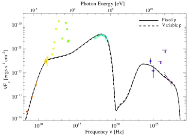
Figure 12: SED of PWN  predicted for the “most likely” combination of model input parameter $\Theta$ for given in Table 11. The observed data points are given in Table 10.

The combination of input parameters $\Theta$ which resulted in the largest ${\mathcal{L}}$ of our MCMC run is given in Table 11, with the value predicted by this combination for each observable given in Table 11 and the predicted SED shown in Figure 12. , our model reproduces most of the properties of  to within $<1\sigma$ of the observed values, with the value predicted by the model deviating by $\sim 1-3\sigma$ from the observed values of $\dot{\theta}_{\rm pwn}$, 327 MHz flux density, 4.8 GHz flux density, and 4.49$-$7.86 GHz spectral index. Notably, this model successfully reproduces the unabsorbed flux and photon index measured in each of the four X-ray bands – unlike many previous attempts of modeling the SED of this source (e.g., Tanaka & Takahara 2011; Torres et al. 2014; Hitomi Collaboration et al. 2018). We note that we did not attempt to reproduce the IR flux density observed from this PWN since, as described in §2.1, emission from surrounding gas dust is likely a significant contributor in this band. As shown in Figure 12, the predicted flux density of the PWN’s synchrotron emission in this band is significantly lower than the observed values (§2.1; Table 2). Furthermore, the expected PWN contribution is not well described by a simple power-law extrapolation of the measured radio or X-ray flux densities.

Table 12: Physical properties of  predicted by the models whose parameters are given in Table 11.

Property	Variable $p$	$p\equiv 1.85690$
Pulsar Age $t_{\rm age}$	1700 years	1700 years
Pulsar Initial Spindown Luminosity $\dot{E}_{0}$	$8.3\times 10^{37}~{}\frac{\rm ergs}{\rm s}$	$5.8\times 10^{37}~{}\frac{\rm ergs}{\rm s}$
Mass of Ejecta Swept-up by PWN $M_{\rm sw,pwn}$	0.85 M⊙	0.73 M⊙
PWN Expansion Velocity $v_{\rm pwn}$	$\approx 610~{}\frac{\rm km}{\rm s}$	$\approx 590~{}\frac{\rm km}{\rm s}$
Ejecta Speed just outside PWN $v_{\rm ej}(R_{\rm pwn})$	$\approx 525~{}\frac{\rm km}{\rm s}$	$\approx 500~{}\frac{\rm km}{\rm s}$
Pulsar Initial Spin Period $P_{0}$	$\approx 50~{}{\rm ms}$	$\approx 51~{}{\rm ms}$
PWN Magnetic Field Strength $B_{\rm pwn}$	$\approx 31~{}\mu{\rm G}$	$\approx 33~{}\mu{\rm G}$

While we have not extensively sampled the possible parameter space and obtained formal uncertainties on the parameters, as done for G54.1+0.3 (Gelfand et al., 2015), the “most likely” parameters identified in our analysis can be used to derive information regarding the formation and underlying physics of this system. As indicated in Table 11, our modeling suggests the progenitor supernova ejected $M_{\rm ej}\approx 11~{}{M}_{\odot}$ of material with a rather low initial kinetic energy $E_{\rm sn}\approx 1.2\times 10^{50}~{}{\rm ergs}$ – a situation where current simulations for core-collapse supernova favor the creation of stellar-mass black hole (e.g., Sukhbold et al. 2016), not a neutron star as observed here. It is important to note that we did center numerous MCMC chains (each consisting of $\approx 50,000$ samples) around a canonical supernova explosion of $M_{\rm ej}\sim 8~{}{M}_{\odot}$ and $E_{\rm sn}\sim 10^{51}~{}{\rm ergs}$ and were unable to reproduce the observed properties of this system in this region of parameter space. As a result, our modeling strongly suggest this system is the result of a low energy, high mass supernova explosion.

This conclusion can be tested by measuring the properties of the supernova ejecta. This is best done by detected thermal X-rays from ejecta heated by the reverse shock. Unfortunately, our results suggest that very little ejecta has interacted with the reverse shock (§4.3). However, as the PWN expands it sweeps up and shocks the inner-most ejecta. For the most likely set of parameters given in Table 11, we find that the PWN has swept-up $M_{\rm sw,pwn}\approx 0.7-0.9~{}{M}_{\odot}$ of ejecta, and is currently expanding ($v_{\rm pwn}-v_{\rm ej}(R_{\rm pwn}))\sim 85-90~{}\frac{\rm km}{\rm s}$ faster than its surroundings . These predictions can be tested with future analysis of the IR emission of this source.

Table 13: Properties of PSR J1833$-$1034 associated with  and other pulsars with either changing braking indices or $p>3$.

Property	PSR J1833$-$1034	PSR J1846$-$0258	PSR B0540-69	PSR J1640$-$4631
Period $P$	$\approx 61.8$ ms	$\approx 327$ ms	$\approx 50.5$ ms	$\approx 206$ ms
Period-Derivative $\dot{P}$	$2.02\times 10^{-13}~{}\frac{\rm s}{\rm s}$	$7.11\times 10^{-12}~{}\frac{\rm s}{\rm s}$	$4.78\times 10^{-13}~{}\frac{\rm s}{\rm s}$	$9.76\times 10^{-13}~{}\frac{\rm s}{\rm s}$
Spin-down Luminosity $\dot{E}$	$3.4\times 10^{37}~{}\frac{\rm ergs}{\rm s}$	$8.1\times 10^{36}~{}\frac{\rm ergs}{\rm s}$	$1.5\times 10^{38}~{}\frac{\rm ergs}{\rm s}$	$4.4\times 10^{36}~{}\frac{\rm ergs}{\rm s}$
Characteristic Age $t_{\rm ch}$	$\approx 4850$ years	$\approx 730$ years	$\approx 1670$ years	$\approx 3350$ years
Surface Dipole Magnetic Field $B_{\rm ns}$	$3.6\times 10^{12}~{}{\rm G}$	$4.9\times 10^{13}~{}{\rm G}$	$5.0\times 10^{12}~{}{\rm G}$	$1.4\times 10^{13}~{}{\rm G}$
Braking Index $p$	$\approx 3.1/\equiv 1.8659$	$2.65/2.16$	$2.13/0.03-0.9$	$3.15\pm 0.03$

The first pulsar with a braking index $p>3$ from a phase-connected timing solution is PSR J1640$-$4631 which has a measured braking index $p=3.15\pm 0.03$ (Archibald et al., 2016). As shown in Table 13, other than age, they are very few physical similarities between these two pulsars: PSR J1833$-$1034 has a period $P\sim 3\times$ smaller than PSR J1640$-$4631, a spin-down luminosity $\dot{E}\sim 10\times$ larger, and a (spin-down inferred) surface dipole magnetic field strength $B_{\rm ns}\sim 4\times$ lower.

In addition, our modeling suggests the age of this system is less than the pulsar’s spin-down timescale ($t_{\rm age}<\tau_{\rm sd}$; Tables 12 & 11), as first suggested by Camilo et al. (2006). As a result, the implied initial spin-down luminosity $\dot{E}_{0}$ (Equation 2) and initial period $P_{0}$ (e.g., Pacini & Salvati 1973; Gaensler & Slane 2006 and references therein):

$$P_{0} = P\left(1+\frac{t_{\rm age}}{\tau_{\rm sd}}\right)^{-\frac{1}{p-1}}$$ (36)

are quite close to their current values (Table 12). The derived initial spin period $P_{0}\approx 50~{}{\rm ms}$ is slightly larger than expected for its surface magnetic field strength by models of fallback onto the proto-neutron star during the supernova (e.g., Watts & Andersson 2002). Furthermore, the inferred initial spin-down luminosity $\dot{E}_{0}$ is somewhat lower than the $\dot{E}_{0}\sim 10^{38}-10^{39}~{}\frac{\rm ergs}{\rm s}$ derived for other systems (e.g., Tanaka & Takahara 2011; Torres et al. 2014; Gelfand et al. 2015).

Extensive trials were conducted with $p_{1}<p_{2}$, but were not able to reproduce the observed properties listed in Table 10. The low values of $p_{1}$ ($p_{1}<2$) inferred for other PWNe have been interpreted as magnetic reconnection dominating particle acceleration at low energies while Fermi acceleration dominating at higher energy (e.g., Sironi & Spitkovsky 2011). However, the required values of $p_{1}$ and $p_{2}$ (Table 11) are both consistent with Fermi acceleration, and their different values possibly suggests particles are accelerated / injected at two sites within this PWN. If correct, this could explain the spatial variations in $\Gamma$ observed near the center of this PWN (e.g., Guest et al. 2019).

Lastly, the results of our modeling can be used to interpret features in the observed SED of this PWN (Figure 12). A particle of energy $E$ will generate synchrotron emission with a power $P_{\rm synch}$ (e.g., Pacholczyk 1970):

$$P_{\rm synch}(E) = \frac{4e^{4}}{9m_{e}^{4}c^{7}}B^{2}E^{2},$$ (37)

where $B$ is the strength of the nebular magnetic field, $e$ and $m_{e}$ are, respectively, the charge and mass of the electron while $c$ is the speed of light, and whose spectrum will peak at a frequency $\nu_{\rm peak}$ (e.g., Pacholczyk 1970):

$$\nu_{\rm peak}(E) = 0.29\times\frac{3}{2}\left(\frac{E}{m_{e}c^{2}}\right)^{2}\frac{eB}{m_{e}c}$$ (38)

For particles with a power-law energy distribution $\frac{dN}{dE}\propto E^{-p_{\rm par}}$, the synchrotron emission is also expected to have a power-law spectrum ($\frac{dN}{dE}\propto E^{-\Gamma}$) with:

$$\alpha = \frac{1-p_{\rm par}}{2}$$ (39)

$$\Gamma = \frac{1+p_{\rm par}}{2}.$$ (40)

This synchrotron emission will cause a particle with energy $E$ to cool in time $t_{\rm cool}$:

$$t_{\rm cool} \equiv \frac{E}{P_{\rm synch}}=\frac{9m_{e}^{4}c^{7}}{4e^{4}}B^{-2}E^{-1}$$ (41)

$$\approx 6.25\left(\frac{B}{1~{}\mu{\rm G}}\right)^{-2}\left(\frac{E}{\rm 1~{}GeV}\right)^{-1}\times 10^{14}~{}{\rm years},$$ (42)

and a break in the electron spectrum will form at the energy $E_{\rm cool}$ whose synchrotron cooling time is equal to the age of the system:

$$E_{\rm cool}(B,t) = \frac{9m_{e}^{4}c^{7}}{4e^{4}}B^{-2}t_{\rm age}^{-1}$$ (43)

$$\approx 1.26\left(\frac{B}{1~{}\mu{\rm G}}\right)^{-2}\left(\frac{t_{\rm age}}{\rm 1~{}yr}\right)^{-1}\times 10^{19}~{}{\rm eV}$$ (44)

For the age $t_{\rm age}$ and current nebular magnetic field strength $B_{\rm pwn}$ predicted by our most likely set of model parameters (Table 12), we have:

$$E_{\rm cool}(B_{\rm pwn},t_{\rm age}) \approx 7.6~{}{\rm TeV}$$ (45)

and $\nu_{\rm peak}(E_{\rm min})\approx 140~{}{\rm GHz}$, $\nu_{\rm peak}(E_{\rm break})\approx 900~{}{\rm THz}$, $h\nu_{\rm peak}(E_{\rm cool})\approx 0.2~{}{\rm keV}$, $h\nu_{\rm peak}(E_{\rm max})\approx 0.1~{}{\rm MeV}$, where $h$ is Planck’s constant. As detailed below, we expect to see features in the observed SED at all of these frequencies.

At $\nu<\nu_{\rm peak}(E_{\rm min})$, the emission will be dominated by “relic particles” injected into the PWN at earlier times and have since (primarily adiabatically) cooled to lower energies. As a result, the “flat” (spectral index $\alpha\approx 0$; flux density $S_{\nu}\propto\nu^{\alpha}$) observed at GeV frequencies does not necessarily reflect the spectrum of injected particles. Beginning at $\nu_{\rm peak}(E_{\rm min})$, the emitting particles will be a mix of freshly injected and “relic” particles, and expect a change in $\alpha$ ($\Gamma$) and this point. However, $t_{\rm cool}\gg t_{\rm age}$ at $\nu_{\rm peak}(E_{\rm min})$ and $\nu_{\rm peak}(E_{\rm break})$, so previously injected particles will dominate in this energy band and the emitted spectrum will be “flatter” than that expected from the freshly injected particles:

$$\alpha_{1} = \frac{1-p_{1}}{2}=-0.93$$ (46)

$$\Gamma_{1} = \frac{1+p_{1}}{2}=1.93.$$ (47)

At photon energy $h\nu\approx h\nu_{\rm peak}(E_{\rm cool})$, radiation from freshly injected particles should begin to dominate the observed emission. This occurs well within the high-energy component of the injected broken power-law spectrum, and the observed synchrotron emission should have:

$$\alpha_{2} \approx \frac{1-p_{2}}{2}=-0.76$$ (48)

$$\Gamma_{2} \approx \frac{1+p_{2}}{2}=1.76.$$ (49)

Indeed, the $\Gamma\sim 1.8-1.9$ measured between $0.8-3.0$ keV (where the emitting particles have $t_{\rm cool}\lesssim t_{\rm age}$) is similar to $\Gamma_{2}=1.76$. At higher photon energies, the shorter cooling time $t_{\rm cool}$ results in a decrease in the average age, and therefore total number, of emitting particles, resulting in a softening (increase in $\Gamma$) of the spectrum. However, due to the decreasing input of energy into the PWN by the pulsar, $\Delta\Gamma\neq 0.5$ as expected from standard synchrotron theory (e.g., Pacholczyk 1970). In fact, our simple model for the evolution of a PWN inside a SNR does a good job of reproducing the increasingly softening spectrum in the X-ray band (Figure 12, Table 10). Lastly, we would expect little synchrotron emission at $h\nu_{\rm peak}(E_{\rm max})\approx 0.1~{}{\mathrm{M}eV}$ – suggesting that  should not produce much MeV emission and therefore is not a promising target for proposed missions like AMEGO.

4.3 SNR shell

The morphology of the SNR rim in  suggests an interaction with dense material in the north. The shell is remarkably circular until an abrupt flattening that results in brightened X-ray emission and enhanced knot-like structures (Figure 1). Spectral investigations by Guest et al. (2019) suggest an ejecta-rich thermal component for which the density is $\sim 45d_{4.6}^{-1/2}f^{-1/2}{\rm\ cm}^{-3}$, where $f$ is the filling factor of the X-ray gas. We note that this value is additionally uncertain due to the unknown composition of the ejecta.

We have investigated a hydrodynamical model for the evolution of the SNR using the results from §4.2 (summarized in Table 11) and assuming the presence of a dramatic density increase in regions north of the explosion center. The simulation was carried out with the grid-based hydrodynamics code VH1 (see Blondin et al. 2001; Kolb et al. 2017), which utilizes the PPMLR method (Colella & Woodward, 1984) to resolve shock propagation. Here we have ignored the contributions from the pulsar since the PWN has no impact on the SNR morphology at this stage of evolution. We ran the simulation to an age of 1700 years (see §4.2), adjusting the position and magnitude of the density jump relative to the explosion center until the observed morphology reproduced that observed for .

We find that a reasonable representation of the SNR morphology can be obtained with a density jump by a factor of $\sim 20$ located $\sim 1.8$ pc north of the explosion center. The results are summarized in Figure 13 where we plot the density distribution from the simulation. The outermost boundary corresponds to the ambient density, and the position of the Forward Shock (FS), Reverse Shock (RS), and Contact Discontinuity (CD) are indicated. The peak density in the northern regions of the SNR is in the reverse-shocked ejecta, where $\rho_{\rm ej}\sim 3.1\times 10^{-23}{\rm\ g\ cm}^{-3}$ ($n\sim 31{\rm\ cm^{-3}}$), in reasonable agreement with the density estimate for the northern knot. While this solution is far from unique, it presents a reasonable interpretation of the basic conditions leading to the observed properties of the SNR. We note that, as expected, the RS (for which the outer contour is overlaid in white) is still far from the PWN boundary ($R_{\rm PWN}\sim 2.4\times 10^{18}{\rm\ cm}$), consistent with our finding in §4.2 that no RS/PWN interaction has occurred.

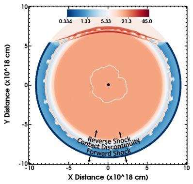
Figure 13: Hydrodynamical simulation of an SNR evolving in a medium with a density jump located to the north of the explosion site. The color bar indicates the density in units of $10^{-24}{\rm\ g\ cm}^{-3}$, and the positions of the Forward Shock, Reverse Shock, and Contact Discontinuity are indicated. The compression in the northern region is similar to that observed in . The white contour corresponds to the outer boundary of the PWN.

5 Summary & Conclusions

We reanalyzed archival IR (Herschel, Spitzer; §2.1) and X-ray (Chandra, NuSTAR, Hitomi; §3.1) observations of PWN . The similar morphology observed in IR emission line and continuum maps of this source suggests surrounding dust and gas produce much of the observed radiation (§4.1). Our analysis of the X-ray observations shows that while there is an overall spectral softening within this band, discrepant power-law parameter values from different detectors indicate instrumental uncertainties should be taken into consideration when interpreting the values (§3.3).

To quantify the degree and shape of the spectral softening in the X-ray band, we separately fit power laws over distinct energy bands (piecewise power law fits §3.2), instead of fitting over the entire detector energy range with a single broken power law. This shape is consistent with what is predicted by models for the evolution of a PWN inside a SNR, which find that the continuous injection of particles into, and changing magnetic field strength inside, the PWN does not result in a sharp break as required by broken power-law models.

We then used a one-zone model for the evolution of a PWN inside a SNR to reproduce the observed dynamical and broadband spectral properties of , taking into consideration that the IR emission is likely not dominated by synchrotron radiation from particles inside the PWN, and the increased uncertainty in the X-ray spectrum resulting from our comparison of different instruments (§4.2). We found that this model can reproduce the properties of this source, but only if the supernova ejecta had a low initial kinetic energy of $E_{\rm sn}\approx 1.2\times 10^{50}~{}{\rm ergs}$ spectrum of particles injected into the PWN at the termination shock is softer at lower energies than at high energies $(p_{1}\approx 2.9>p_{2}\approx 2.5)$ – opposite of what is observed from most other PWNe. Both values are consistent with what is expected from diffusive shock acceleration, suggesting that magnetic reconnection may not play an important role in accelerating particles in this PWN, and the different values may indicate two different acceleration sites. Furthermore, we used a hydrodynamical model to determine the structure of the ambient medium needed to reproduce the morphology of the observed SNR shell (§4.3). We are able to do so if there is a $\sim 20\times$ increase in density ${\sim}1.8$ pc north of the explosion center.

As a result, we have obtained an extensive picture of the supernova, neutron star, pulsar wind, and surrounding material of this source. The derived properties are useful for understanding how neutron stars are created in core-collapse supernovae and the different ways they energize their environment. The techniques and tools presented in this study are applicable when analyzing many other PWNe, and their use may provide a more comprehensive view of the different mechanisms by which neutron stars are formed and produce some of the highest energy particles in the Universe.

Appendix A Systematic Errors in NuSTAR Spectrum

Figure 14: Photon index (a), normalization (b), and reduced $\chi^{2}$ (c) for each observation over the entire energy range (3–45 keV). The fitted model is with the black-body component. Shaded regions indicate 90% confidence intervals.

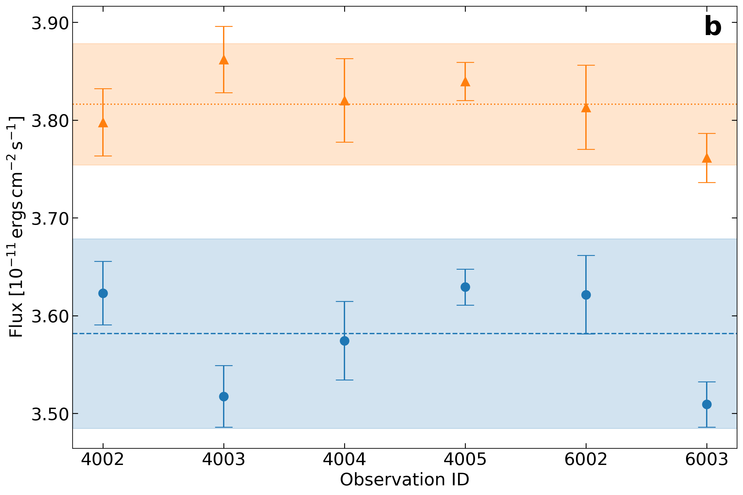
Figure 15: Photon index, normalization, and reduced $\chi^{2}$ for each observation in the energy bands: 3–8 keV (a, b, c), 8–20 keV (d, e, f), 20–45 keV (g, h, i). The fitted model is with the black-body component. Shaded regions indicate 90% confidence intervals.

Here we discuss the systematic differences between FPMA and FPMB spectra. We initially fit all twelve NuSTAR spectra independently over the entire 3–45 keV range without dividing the energy ranges (Figure 14) using the model with the pulsar black-body component (explained in §3.1). While we also fit the model without the pulsar black-body component and obtained similar results, here we only report on the results of fitting the model with the pulsar black-body component as we are simply trying to highlight the differences between FPMA and FPMB spectra.

We found that the photon index $\Gamma$ was consistently higher for FPMA spectra compared to FPMB spectra, indicating spectra from FPMA was softer (i.e., a lower fraction of higher energy X-ray photons). The weighted average (inverse variance weighting), across observations, of the photon index for spectra from FPMA was $\Gamma_{\mathrm{A}}=2.12\pm 0.01$ and the weighted average of of the photon index for spectra from FPMB was $\Gamma_{\mathrm{B}}=2.09\pm 0.01$. The uncertainties reported here are the $1\sigma$ weighted sample standard deviations calculated with the formula $\sigma=\sqrt{\frac{N}{N-1}\frac{\Sigma_{i}w_{i}(x_{i}-\bar{x})^{2}}{\Sigma_{i}w_{i}}}$ where $w_{i}\equiv 1/\sigma_{i}^{2}$, $\bar{x}$ is the weighted average, and $N=6$ (the number of observations) in our case. The standard deviation of $\pm 0.01$ for each photon index is within what is mentioned as the approximate repeatability error of the spectral slope ($\pm 0.01$) in the NuSTAR calibration paper (Madsen et al., 2015), indicating that the discrepancy across different observations from each FPM is within the calibration uncertainty. While Madsen et al. (2015) report offsets of $\Delta\Gamma\approx 0.1$ between $\Gamma_{\mathrm{A}}$ and $\Gamma_{\mathrm{B}}$ for the source 3C273 during certain cross-calibration campaign observations, they do not address $\Gamma_{\mathrm{A}}$ being consistently higher than $\Gamma_{\mathrm{B}}$, which is what we observe for . They do note that if the signal to noise ratio is high enough, which could be the case for a bright source such as , the inter-instrumental slope differences between FPMA and FPMB could be significant.

In addition to the discrepancy in the photon indices between FPMA and FPMB spectra, the unabsorbed flux values in the 3–45 keV range are also different. In units of $10^{-11}$ erg s^-1 cm^-2 , we obtain $F_{\mathrm{A(3-45)}}=9.02\pm 0.14$ and $F_{\mathrm{B(3-45)}}=9.84\pm 0.04$. The two weighted average flux values differ by $\sim 8\%$, which is slightly larger than the potential $5\%$ flux difference mentioned in the NuSTAR calibration paper (Madsen et al., 2015). We find that the unabsorbed flux for spectra from FPMB is consistently higher than that of spectra from FPMA. As with the photon index, this consistent offset may be due to the brightness of .

We then repeated the above analysis over each energy band; 3–8 keV, 8–20 keV, and 20–45 keV (Figure 15). The photon indices $\Gamma_{\mathrm{A}},\Gamma_{\mathrm{B}}$ agree in the 3–8 keV band and there is no consistent offset. However, while the 90% confidence intervals overlap for the 8–20 keV and 20–45 keV bands, we do see that in most cases $\Gamma_{\mathrm{A}}$ is higher than $\Gamma_{\mathrm{B}}$. For the unabsorbed flux we see that the value is consistently higher for FPMB spectra compared to FPMA spectra in all energy bands. The 90% confidence intervals for the unabsorbed flux do not overlap in the 3–8 keV and 8–20 keV bands, and slightly overlap in the 20–45 keV band due to the large spread of values for FPMB spectra.

While there exist discrepancies in the PWN photon index and unabsorbed flux values between the spectra from FPMA and FPMB, the fit results between spectra from the same FPM across different observations are within the calibration uncertainty. As such, we believe the appropriate approach is to do joint fits of spectra from each FPM separately.

References

- Abdo et al. (2013) Abdo, A. A., Ajello, M., Allafort, A., et al. 2013, ApJS, 208, 17
- Ajello et al. (2017) Ajello, M., Atwood, W. B., Baldini, L., et al. 2017, ApJS, 232, 18
- Altenhoff et al. (1970) Altenhoff, W. J., Downes, D., Goad, L., Maxwell, A., & Rinehart, R. 1970, A&AS, 1, 319
- Amato (2020) Amato, E. 2020, The theory of Pulsar Wind Nebulae: recent progress, , , arXiv:2001.04442
- Archibald et al. (2016) Archibald, R. F., Gotthelf, E. V., Ferdman, R. D., et al. 2016, ApJ, 819, L16
- Arnaud (1996) Arnaud, K. A. 1996, in Astronomical Society of the Pacific Conference Series, Vol. 101, Astronomical Data Analysis Software and Systems V, ed. G. H. Jacoby & J. Barnes, 17
- Arons (2004) Arons, J. 2004, Advances in Space Research, 33, 466
- Baade & Zwicky (1934) Baade, W., & Zwicky, F. 1934, Proceedings of the National Academy of Science, 20, 254
- Becker & Szymkowiak (1981) Becker, R. H., & Szymkowiak, A. E. 1981, ApJ, 248, L23
- Bhatnagar et al. (2011) Bhatnagar, S., Rau, U., Green, D. A., & Rupen, M. P. 2011, ApJ, 739, L20
- Bietenholz & Bartel (2008) Bietenholz, M. F., & Bartel, N. 2008, MNRAS, 386, 1411
- Bietenholz et al. (2011) Bietenholz, M. F., Matheson, H., Safi-Harb, S., Brogan, C., & Bartel, N. 2011, MNRAS, 412, 1221
- Blondin et al. (2001) Blondin, J. M., Chevalier, R. A., & Frierson, D. M. 2001, ApJ, 563, 806
- Bock et al. (2001) Bock, D. C. J., Wright, M. C. H., & Dickel, J. R. 2001, ApJ, 561, L203
- Camilo et al. (2006) Camilo, F., Ransom, S. M., Gaensler, B. M., et al. 2006, ApJ, 637, 456
- Cash (1979) Cash, W. 1979, ApJ, 228, 939
- Chevalier (2005) Chevalier, R. A. 2005, ApJ, 619, 839
- Colella & Woodward (1984) Colella, P., & Woodward, P. R. 1984, Journal of Computational Physics, 54, 174
- Doe et al. (2007) Doe, S., Nguyen, D., Stawarz, C., et al. 2007, in Astronomical Society of the Pacific Conference Series, Vol. 376, Astronomical Data Analysis Software and Systems XVI, ed. R. A. Shaw, F. Hill, & D. J. Bell, 543
- Ferdman et al. (2015) Ferdman, R. D., Archibald, R. F., & Kaspi, V. M. 2015, ApJ, 812, 95
- Fixsen (2009) Fixsen, D. J. 2009, ApJ, 707, 916
- Freeman et al. (2001) Freeman, P., Doe, S., & Siemiginowska, A. 2001, in Society of Photo-Optical Instrumentation Engineers (SPIE) Conference Series, Vol. 4477, Astronomical Data Analysis, ed. J.-L. Starck & F. D. Murtagh, 76–87
- Fruscione et al. (2006) Fruscione, A., McDowell, J. C., Allen, G. E., et al. 2006, in Society of Photo-Optical Instrumentation Engineers (SPIE) Conference Series, Vol. 6270, Society of Photo-Optical Instrumentation Engineers (SPIE) Conference Series, 62701V
- Gaensler & Slane (2006) Gaensler, B. M., & Slane, P. O. 2006, ARA&A, 44, 17
- Gallant & Tuffs (1999) Gallant, Y. A., & Tuffs, R. J. 1999, in ESA Special Publication, Vol. 427, The Universe as Seen by ISO, ed. P. Cox & M. Kessler, 313
- Gelfand et al. (2013) Gelfand, J., Slane, P., & Temim, T. 2013, in The Fast and the Furious: Energetic Phenomena in Isolated Neutron Stars, Pulsar Wind Nebulae and Supernova Remnants, ed. J. U. Ness, 24
- Gelfand (2017) Gelfand, J. D. 2017, Astrophysics and Space Science Library, Vol. 446, Radiative Models of Pulsar Wind Nebulae, ed. D. F. Torres, 161
- Gelfand et al. (2015) Gelfand, J. D., Slane, P. O., & Temim, T. 2015, ApJ, 807, 30
- Gelfand et al. (2009) Gelfand, J. D., Slane, P. O., & Zhang, W. 2009, ApJ, 703, 2051
- Goodman & Weare (2010) Goodman, J., & Weare, J. 2010, Communications in Applied Mathematics and Computational Science, 5, 65
- Gotthelf et al. (2014) Gotthelf, E. V., Tomsick, J. A., Halpern, J. P., et al. 2014, ApJ, 788, 155
- Guest et al. (2019) Guest, B. T., Safi-Harb, S., & Tang, X. 2019, MNRAS, 482, 1031
- H. E. S. S. Collaboration et al. (2018) H. E. S. S. Collaboration, Abdalla, H., Abramowski, A., et al. 2018, A&A, 612, A1
- Harrison et al. (2013) Harrison, F. A., Craig, W. W., Christensen, F. E., et al. 2013, ApJ, 770, 103
- Hitomi Collaboration et al. (2018) Hitomi Collaboration, Aharonian, F., Akamatsu, H., et al. 2018, PASJ, 70, 38
- Hunter (2007) Hunter, J. D. 2007, Computing in Science & Engineering, 9, 90
- Joye & Mandel (2003) Joye, W. A., & Mandel, E. 2003, in Astronomical Society of the Pacific Conference Series, Vol. 295, Astronomical Data Analysis Software and Systems XII, ed. H. E. Payne, R. I. Jedrzejewski, & R. N. Hook, 489
- Kim & An (2019) Kim, M., & An, H. 2019, Journal of Korean Astronomical Society, 52, 41
- Kolb et al. (2017) Kolb, C., Blondin, J., Slane, P., & Temim, T. 2017, ApJ, 844, 1
- Koo et al. (2016) Koo, B.-C., Lee, J.-J., Jeong, I.-G., Seok, J. Y., & Kim, H.-J. 2016, ApJ, 821, 20
- Livingstone et al. (2011) Livingstone, M. A., Ng, C. Y., Kaspi, V. M., Gavriil, F. P., & Gotthelf, E. V. 2011, ApJ, 730, 66
- Madsen et al. (2020) Madsen, K. K., Grefenstette, B. W., Pike, S., et al. 2020, NuSTAR low energy effective area correction due to thermal blanket tear, , , arXiv:2005.00569
- Madsen et al. (2015) Madsen, K. K., Harrison, F. A., Markwardt, C. B., et al. 2015, ApJS, 220, 8
- Marshall et al. (2016) Marshall, F. E., Guillemot, L., Harding, A. K., Martin, P., & Smith, D. A. 2016, ApJ, 827, L39
- Martín et al. (2012) Martín, J., Torres, D. F., & Rea, N. 2012, MNRAS, 427, 415
- Matheson & Safi-Harb (2010) Matheson, H., & Safi-Harb, S. 2010, ApJ, 724, 572
- Metropolis (1985) Metropolis, N. 1985, Monte-Carlo: In the Beginning and Some Great Expectations, ed. R. Alcouffe, R. Dautray, A. Forster, G. Ledonois, & B. Mercier, Vol. 240, 62
- Nakajima et al. (2018) Nakajima, H., Maeda, Y., Uchida, H., et al. 2018, PASJ, 70, 21
- NASA High Energy Astrophysics Science Archive Research Center (2014) (HEASARC) NASA High Energy Astrophysics Science Archive Research Center (HEASARC). 2014, HEAsoft: Unified Release of FTOOLS and XANADU, , , ascl:1408.004
- Nynka et al. (2014) Nynka, M., Hailey, C. J., Reynolds, S. P., et al. 2014, ApJ, 789, 72
- Oliphant (2006) Oliphant, T. E. 2006, A guide to NumPy, Vol. 1 (Trelgol Publishing USA)
- Ott (2010) Ott, S. 2010, in Astronomical Society of the Pacific Conference Series, Vol. 434, Astronomical Data Analysis Software and Systems XIX, ed. Y. Mizumoto, K. I. Morita, & M. Ohishi, 139
- Ou et al. (2016) Ou, Z. W., Tong, H., Kou, F. F., & Ding, G. Q. 2016, MNRAS, 457, 3922
- Pacholczyk (1970) Pacholczyk, A. G. 1970, Radio astrophysics. Nonthermal processes in galactic and extragalactic sources
- Pacini & Salvati (1973) Pacini, F., & Salvati, M. 1973, ApJ, 186, 249
- Planck Collaboration et al. (2016) Planck Collaboration, Arnaud, M., Ashdown, M., et al. 2016, A&A, 586, A134
- Poglitsch et al. (2010) Poglitsch, A., Waelkens, C., Geis, N., et al. 2010, A&A, 518, L2
- Ranasinghe & Leahy (2018) Ranasinghe, S., & Leahy, D. A. 2018, AJ, 155, 204
- Reynolds & Chevalier (1984) Reynolds, S. P., & Chevalier, R. A. 1984, ApJ, 278, 630
- Roy et al. (2012) Roy, J., Gupta, Y., & Lewandowski, W. 2012, MNRAS, 424, 2213
- Salter et al. (1989a) Salter, C. J., Emerson, D. T., Steppe, H., & Thum, C. 1989a, A&A, 225, 167
- Salter et al. (1989b) Salter, C. J., Reynolds, S. P., Hogg, D. E., Payne, J. M., & Rhodes, P. J. 1989b, ApJ, 338, 171
- Sironi & Spitkovsky (2011) Sironi, L., & Spitkovsky, A. 2011, ApJ, 741, 39
- Sironi et al. (2013) Sironi, L., Spitkovsky, A., & Arons, J. 2013, ApJ, 771, 54
- Slane (2017) Slane, P. 2017, Pulsar Wind Nebulae, ed. A. W. Alsabti & P. Murdin, 2159
- Smithsonian Astrophysical Observatory (2000) Smithsonian Astrophysical Observatory. 2000, SAOImage DS9: A utility for displaying astronomical images in the X11 window environment, , , ascl:0003.002
- Sukhbold et al. (2016) Sukhbold, T., Ertl, T., Woosley, S. E., Brown, J. M., & Janka, H. T. 2016, ApJ, 821, 38
- Sun et al. (2011) Sun, X. H., Reich, P., Reich, W., et al. 2011, A&A, 536, A83
- Takahashi et al. (2014) Takahashi, T., Mitsuda, K., Kelley, R., et al. 2014, in Society of Photo-Optical Instrumentation Engineers (SPIE) Conference Series, Vol. 9144, Proc. SPIE, 914425
- Takahashi et al. (2016) Takahashi, T., Kokubun, M., Mitsuda, K., et al. 2016, Society of Photo-Optical Instrumentation Engineers (SPIE) Conference Series, Vol. 9905, The ASTRO-H (Hitomi) x-ray astronomy satellite, 99050U
- Tanaka & Takahara (2011) Tanaka, S. J., & Takahara, F. 2011, ApJ, 741, 40
- Torres (2017) Torres, D. F. 2017, Modelling Pulsar Wind Nebulae, Vol. 446, doi:10.1007/978-3-319-63031-1
- Torres et al. (2014) Torres, D. F., Cillis, A., Martín, J., & de Oña Wilhelmi, E. 2014, Journal of High Energy Astrophysics, 1, 31
- Van Der Walt et al. (2011) Van Der Walt, S., Colbert, S. C., & Varoquaux, G. 2011, Computing in Science & Engineering, 13, 22
- Virtanen et al. (2020) Virtanen, P., Gommers, R., Oliphant, T. E., et al. 2020, Nature Methods, 17, 261
- Wang et al. (2020) Wang, L. J., Ge, M. Y., Wang, J. S., et al. 2020, MNRAS, 494, 1865
- Watts & Andersson (2002) Watts, A. L., & Andersson, N. 2002, MNRAS, 333, 943
- Wik et al. (2014) Wik, D. R., Hornstrup, A., Molendi, S., et al. 2014, ApJ, 792, 48
- Wilms et al. (2000) Wilms, J., Allen, A., & McCray, R. 2000, ApJ, 542, 914
- Wilson & Altenhoff (1970) Wilson, T. L., & Altenhoff, W. 1970, Astrophys. Lett., 5, 47
- Yang et al. (2016) Yang, G., Brandt, W. N., Luo, B., et al. 2016, ApJ, 831, 145