A new life of Pearson’s skewness

Abstract

In this work we show how coupling and stochastic dominance methods can be successfully applied to a classical problem of rigorizing Pearson’s skewness. Here, we use Fréchet means to define generalized notions of positive and negative skewness that we call truly positive and truly negative. Then, we apply stochastic dominance approach in establishing criteria for determining whether a continuous random variable is truly positively skewed. Intuitively, this means that scaled right tail of the probability density function exhibits strict stochastic dominance over equivalently scaled left tail. Finally, we use the stochastic dominance criteria and establish some basic examples of true positive skewness, thus demonstrating how the approach works in general.

1 Introduction

Consider a positively skewed (right-skewed) unimodal distribution with finite second moment. It is expected that the mode, the median, and the mean line up in an increasing order, i.e.,

$$\mathrm{mode}~{}<~{}\mathrm{median}~{}<~{}\mathrm{mean}.$$

Symmetrically, for a negatively skewed (left-skewed) unimodal distribution with finite second moment,

$$\mathrm{mean}~{}<~{}\mathrm{median}~{}<~{}\mathrm{mode}.$$

Here, when saying that a distribution is positively skewed we usually mean Pearson’s moment coefficient of skewness (the standardized third central moment) is positive. However, there are notable exceptions to the above orderings, also known as the mean-median-mode inequalities. See [1, 17]. It all depends on how we measure skewness. Indeed, there are other measurements of skewness besides the moment coefficient such as Pearson’s first skewness coefficient also known as mode skewness defined as

$${\mathrm{mean}-\mathrm{mode}\over\mathrm{standard~{}deviation}}$$

and Pearson’s second skewness coefficient also known as median skewness defined as

$$3\times{\mathrm{mean}-\mathrm{median}\over\mathrm{standard~{}deviation}}.$$

The sign of the latter two measurements of skewness is consistent with the above discussed ordering of the mode, the median, and the mean.

Thus, whether the signs of the mode skewness, the median skewness, and the moment coefficient of skewness align depends on how we define skewness. First, we need an approach that unifies the different measurements of skewness in determining the sign of skewness (this is done in Def. 3 and 4 below). Second, when defining positive skewness, the objective is to characterize the distributions for which the left tail is “spreading short” and the right tail is “spreading longer”. If looking at this problem from the stochastic dominance perspective, we want to dissect the distribution into the left and the right parts so that when we reflect the left part, align both at zero, and multiply each by a certain monotone function (positive constant times a power of $x$) so that each part is converted into a distribution over positive half-line. If the distribution obtained from the right part exhibits stochastic dominance over the distribution obtained from the left part, then this should imply that the left tail is “spreading short” and the right tail is “spreading longer”. Hence, such distribution is positively skewed (reverse left and right for the negatively skewed distributions). Thus it is natural to consider finding criteria for the skewness to be positive or negative that is based on stochastic dominance of one tail over the other. Definition 3 of true positive skewness and its variation Def. 4 for unimodal distributions yield such stochastic dominance criteria which we establish in Sect. 2, and apply in Sect. 3.

We will generalize positive and negative skewness by consider the following class of centroids known as Fréchet $p$-means [4].

Definition 1.

For $p\in[1,\infty)$ and a random variable $X$ with the finite $p$-th moment, the quantity

$$\nu_{p}={\rm argmin}_{a\in\mathbb{R}}E\big{[}|X-a|^{p}\big{]}$$ (1)

is called Fréchet $p$-mean, or simply the $p$-mean.

The theoretical $p$-mean $\nu_{p}$ is uniquely defined for all $p\geq 1$ as $E\big{[}|X-a|^{p}\big{]}$ is a strictly convex function of $a$. Moreover, the $p$-mean $\nu_{p}$ is a unique solution of

$$E\big{[}(X-\nu_{p})_{+}^{p-1}\big{]}=E\big{[}(\nu_{p}-X)_{+}^{p-1}\big{]}.$$ (2)

Notice that (2) can be used as an extended definition of the $p$-mean that only requires finiteness of the $(p-1)$-st moment.

Definition 2.

For $p\in[1,\infty)$ and a continuous random variable $X$ with the finite $(p-1)$-st moment, the unique solution $\nu_{p}$ of (2) is the $p$-mean of $X$.

For the rest of the paper the $p$-mean $\nu_{p}$ of $X$ is as defined in Def. 2, and we let

$$\mathcal{D}=\big{\{}p\geq 1\,:\,E[|X|^{p-1}]<\infty\big{\}}$$

denote the domain of $\nu_{p}$. Next, we observe that $\nu_{1}$ and $\nu_{2}$ are respectively the median (in continuous case) and the mean of $X$. If the distribution of $X$ is unimodal, we let $\nu_{0}$ denote the mode. In the unimodal case, we will use the domain $\,\mathcal{D}_{0}=\mathcal{D}\cup\{0\}$.

For $p\in(0,1)$, there are examples of no uniqueness of $\nu_{p}$ in (1). For instance, if $X$ is a Bernoulli random variable with parameter $1/2$, there will be two values of $\nu_{p}$ for each $p\in(0,1)$. In Sect. 4, we will observe that often Definition 2 can be extended to include $p\in(0,1)$.

Next, we observe that the $p$-means $\nu_{0}$, $\nu_{1}$, $\nu_{2}$, and $\nu_{4}$ are definitive for the notion of positive skewness defined via the Pearson’s first and second skewness coefficients, as well as the Pearson’s moment coefficient of skewness. Indeed, Karl Pearson’s first skewness coefficient (mode skewness) for a unimodal random variable is expressed as ${\nu_{2}-\nu_{0}\over\sigma}$, where $\sigma$ denotes the standard deviation, while Pearson’s second skewness coefficient (median skewness) is given by ${3(\nu_{2}-\nu_{1})\over\sigma}$. Finally, the renown Pearson’s moment coefficient of skewness

$$\gamma=E\left[\left({X-\nu_{2}\over\sigma}\right)^{3}\right]$$

is also related to the $p$-means via the following proposition.

Proposition 1.

Consider a random variable $X$ with a finite third moment. The Pearson’s moment coefficient of skewness $\gamma$ is positive if and only if $\nu_{4}>\nu_{2}$.

Proof.

Notice that the following cubic equation in $a$,

$$E\big{[}(X-a)^{3}\big{]}=0,$$ (3)

can be rewritten as

$$(a-\nu_{2})^{3}+3\sigma^{2}(a-\nu_{2})-\sigma^{3}\gamma=0.$$ (4)

The 4-mean $\nu_{4}$ is the only real root of (3), and thus of (4). Therefore, $\nu_{4}$ is now being obtained from (4) as follows:

$$\gamma=\left({\nu_{4}-\nu_{2}\over\sigma}\right)^{3}+3\left({\nu_{4}-\nu_{2}\over\sigma}\right).$$ (5)

∎

Throughout the rest of the paper, we consider a continuous random variable $X$ with density function $f(x)$. Furthermore, we suppose $f(x)$ has support $supp(f)=(L,R)$, where $L$ may take value at $-\infty$ and $R$ may take value at $\infty$.

By Proposition 1, the second skewness coefficient and the moment coefficient of skewness are both positive if and only if

$$\nu_{1}~{}<~{}\nu_{2}~{}<~{}\nu_{4}.$$

In the case of unimodal continuous distribution, both, the moment coefficient of skewness is positive and the mean-median-mode inequality holds if and only if

$$\nu_{0}~{}<~{}\nu_{1}~{}<~{}\nu_{2}~{}<~{}\nu_{4}.$$

See Fig. 1. This observation suggests the notion of true positive skewness defined below.

Definition 3.

We say that a random variable $X$, or its distribution, is truly positively skewed if and only if $\nu_{p}$ is an increasing function of $p$ in the domain $\mathcal{D}$, provided the interior of $\mathcal{D}$ is nonempty. Analogously, $X$ is truly negatively skewed if and only if $\nu_{p}$ is a decreasing function of $p$ in $\mathcal{D}$.

The above defined true positive skewness insures $\,\nu_{1}\,<\,\nu_{2}\,<\,\nu_{4}$.

Definition 4.

We say that a unimodal distribution is truly mode positively skewed if and only if $\nu_{p}$ is an increasing function of $p$ in the domain $\mathcal{D}_{0}$. Analogously, it is truly mode negatively skewed if and only if $\nu_{p}$ is a decreasing function of $p$ in $\mathcal{D}_{0}$.

Observe that true mode positive skewness guarantees $\,\nu_{0}\,<\,\nu_{1}\,<\,\nu_{2}\,<\,\nu_{4}$. Notice also that a distribution can be truly positively skewed or truly mode positively skewed even in the absence of finite second moment.

Besides obtaining the sign of skewness, Definitions 3 and 4 do not immediately provide a way of measuring the magnitude of skewness. Defining the corresponding measures of skewness and extending the approach to multidimensional distributions is touched upon in the discussion section (Sect. 5). Importantly, this theoretical work concentrates on the problem of rigorously defining the sign of skewness. We do not intend to venture into statistical analysis or statistical applications of here defined concepts. In general, the question of centroids and their role in rigorously defining skewness that we considered in this paper has a long and interesting history; see for example [7, 16, 19, 20, 12, 5, 6, 3, 2]. Yet, this problem can still generate new challenges for theoretical probabilists and statisticians alike.

In this paper we will show how true positive skewness (and analogously, true negative skewness) can be validated using the methods of coupling and stochastic dominance. These methods are widely used in statistical mechanics and interacting particle systems, the theory of mixing times, and beyond. See [8, 9, 10, 11, 13] and references therein. Specifically we will need the following well known result.

Lemma 1 ([11, 13]).

Suppose $X$ and $Y$ are real valued random variables with cumulative distribution functions denoted by $F_{X}$ and $F_{Y}$ respectively and satisfying $F_{X}(x)\geq F_{Y}(x)$, i.e., $Y$ exhibits stochastic dominance over $X$, then, for any increasing function $h:\mathbb{R}\rightarrow\mathbb{R}$ we have $E[h(Y)]\geq E[h(X)]$. Moreover, if $F_{X}\not\equiv F_{Y}$, i.e., $Y$ exhibits strict stochastic dominance over $X$, and if $h(x)$ is strictly increasing, then $E[h(Y)]>E[h(X)]$.

Lemma 1 is usually proved via a coupling argument. If $X$ and $Y$ are continuous random variables, the inequality in Lemma 1 follows from the integration by parts. In some instances, instead of stating that one random variable exhibits (strict) stochastic dominance over another, it is more convenient to say that one distribution or p.d.f. exhibits (strict) stochastic dominance over the other.

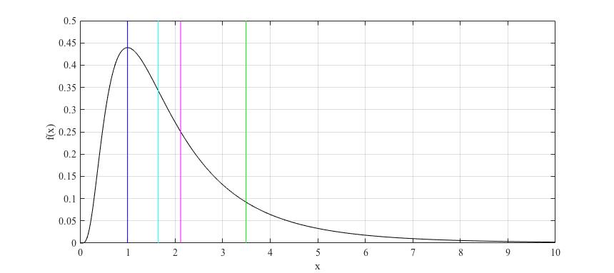
Figure 1: For the log-normal density function with parameters $\mu=\sigma^{2}=1/2$ and p.d.f. $\,f(x)={1\over\sqrt{\pi}x}\exp\left\{-(\log{x}-1/2)^{2}\right\}$, we have the following centroids indicated on the plot: the mode $\,\nu_{0}=\exp\left\{\mu-\sigma^{2}\right\}=1$, the median $\,\nu_{1}=\exp\left\{\mu\right\}=e^{1/2}$, the mean $\,\nu_{2}=\exp\left\{\mu+{\sigma^{2}\over 2}\right\}=e^{3/4}$, and the $4$-mean $\,\nu_{4}=\exp\left\{\mu+{3\sigma^{2}\over 2}\right\}=e^{5/4}$.

Before presenting the general approach in Sect. 2, we show how stochastic dominance method can be used to establish true positive skewness of exponential random variables.

Example 1 (Exponential distribution).

Consider an exponential random variable $X$ with parameter $\lambda>0$. Without loss of generality let $\lambda=1$. Equation (2) implies

$$\int\limits_{0}^{\nu_{p}}(\nu_{p}-x)^{p-1}e^{-x}\,dx\,=\int\limits_{\nu_{p}}^{\infty}(x-\nu_{p})^{p-1}e^{-x}\,dx.$$

This simplifies to

$$\int\limits_{0}^{\nu_{p}}x^{p-1}e^{x}\,dx=\Gamma(p).$$ (6)

Differentiating ${d\over dp}$ in (6) yields

$$\nu_{p}^{p-1}e^{\nu_{p}}\,{d\nu_{p}\over dp}\,+\int\limits_{0}^{\nu_{p}}x^{p-1}e^{x}\,\log{x}\,dx\,=\int\limits_{0}^{\infty}x^{p-1}\,e^{-x}\,\log{x}\,dx$$ (7)

Next, we observe that the gamma distribution with the p.d.f. ${1\over\Gamma(p)}x^{p-1}\,e^{-x}{\bf 1}_{(0,\infty)}(x)$ stochastically dominates the distribution with the p.d.f. ${1\over\Gamma(p)}x^{p-1}\,e^{x}{\bf 1}_{(0,\nu_{p})}(x)$. Thus, Lemma 1 implies

$$\int\limits_{0}^{\nu_{p}}x^{p-1}e^{x}\,\log{x}\,dx\,<\int\limits_{0}^{\infty}x^{p-1}\,e^{-x}\,\log{x}\,dx$$ (8)

as $\log{x}$ is an increasing function. Consequently, equations (7) and (8) imply ${d\nu_{p}\over dp}>0$ for all $p>0$. Hence, exponential random variables are proved to be truly positively skewed (Def. 3) and, as the mode $\nu_{0}=0$, truly mode positively skewed (Def. 4).

2 True positive skewness via stochastic dominance

For a given $p\in\mathcal{D}$, the theoretical $p$-mean $\nu_{p}$ defined in (2) solves

$$H_{p}:=\int\limits_{0}^{\nu_{p}-L}x^{p-1}\,f(\nu_{p}-x)\,dx=\int\limits_{0}^{R-\nu_{p}}x^{p-1}\,f(\nu_{p}+x)\,dx.$$ (9)

Next, we state and prove a criterion for $\nu_{p}$ to be increasing, and therefore for the p.d.f. $f(x)$ to be truly positively skewed.

Theorem 1.

Consider a continuous random variable with p.d.f. $f(x)$ supported on $supp(f)=(L,R)$, and a real number $p$ in the interior of $\mathcal{D}$. If p.d.f. ${1\over H_{p}}x^{p-1}\,f(\nu_{p}+x){\bf 1}_{(0,R-\nu_{p})}(x)$ exhibits strict stochastic dominance over p.d.f. ${1\over H_{p}}x^{p-1}\,f(\nu_{p}-x){\bf 1}_{(0,\nu_{p}-L)}(x)$, then function $\nu_{p}$ is increasing at $p$. Consequently, if the above stochastic dominance holds for all $p$ in the interior of $\mathcal{D}$, the distribution is truly positively skewed (Def. 3).

Proof.

For $p$ in the interior of $\mathcal{D}$, we use Leibniz integral rule to obtain

$$0= {d\over dp}\left(\int\limits_{L}^{\nu_{p}}(\nu_{p}-x)^{p-1}\,f(x)\,dx~{}-\int\limits_{\nu_{p}}^{R}(x-\nu_{p})^{p-1}\,f(x)\,dx\right)$$

$$= \left((p-1)\int\limits_{L}^{\nu_{p}}(\nu_{p}-x)^{p-2}\,f(x)\,dx~{}+\int\limits_{L}^{\nu_{p}}(\nu_{p}-x)^{p-1}\,f(x)\,dx\right){d\nu_{p}\over dp}$$

$$\quad+\left((p-1)\int\limits_{\nu_{p}}^{R}(x-\nu_{p})^{p-2}\,f(x)\,dx~{}-\int\limits_{\nu_{p}}^{R}(x-\nu_{p})^{p-1}\,f(x)\,dx\right){d\nu_{p}\over dp}$$

$$\quad+\int\limits_{0}^{\nu_{p}-L}x^{p-1}\,\log{x}\,f(\nu_{p}-x)\,dx~{}-~{}\int\limits_{0}^{R-\nu_{p}}x^{p-1}\,\log{x}\,f(\nu_{p}+x)\,dx,$$

which simplifies to

$${d\nu_{p}\over dp}={\int\limits_{0}^{R-\nu_{p}}x^{p-1}\,\log{x}\,f(\nu_{p}+x)\,dx-\int\limits_{0}^{\nu_{p}-L}x^{p-1}\,\log{x}\,f(\nu_{p}-x)\,dx\over(p-1)\left[\int\limits_{0}^{\nu_{p}-L}x^{p-2}f(\nu_{p}-x)dx+\int\limits_{0}^{R-\nu_{p}}x^{p-2}f(\nu_{p}+x)\big{]}dx\right]}.$$ (10)

Under the strict stochastic dominance assumption of the theorem, Lemma 1 implies

$$\int\limits_{0}^{R-\nu_{p}}x^{p-1}\,\log{x}\,f(\nu_{p}+x)\,dx~{}>~{}\int\limits_{0}^{\nu_{p}-L}x^{p-1}\,\log{x}\,f(\nu_{p}-x)\,dx.$$ (11)

Together, equations (10) and (11) imply ${d\nu_{p}\over dp}>0$ for all $p$ in the interior of $\mathcal{D}$. ∎

Remark 1.

Returning to the discussion in the introduction of this paper (Sec. 1), Thm. 1 states that if we dissect $f(x)$ at $\nu_{p}$ into the left and the right parts so that when we reflect the left part, and align both at zero, and multiply each by ${1\over H_{p}}x^{p-1}$, then each part is converted into a distribution over positive half-line, i.e., densities ${1\over H_{p}}x^{p-1}\,f(\nu_{p}-x){\bf 1}_{(0,\nu_{p}-L)}(x)$ and ${1\over H_{p}}x^{p-1}\,f(\nu_{p}+x){\bf 1}_{(0,R-\nu_{p})}(x)$. If p.d.f. ${1\over H_{p}}x^{p-1}\,f(\nu_{p}+x){\bf 1}_{(0,R-\nu_{p})}(x)$ obtained from the right part exhibits stochastic dominance over p.d.f. ${1\over H_{p}}x^{p-1}\,f(\nu_{p}-x){\bf 1}_{(0,\nu_{p}-L)}(x)$ obtained from the left part, then this should imply that the left tail is “spreading short” and the right tail is “spreading longer”. Hence, such distribution is truly positively skewed.

Importantly, this stochastic dominance argument remains valid and true positive skewness can be established even in the case of a distribution with infinite first moment and $\,\mathcal{D}\subseteq[1,2)$. See Pareto distribution example in Sect. 3.4. This is one of the advantages of using Def. 3 and 4 in determining the sign of skewness.

Next, we present a criterion for the p.d.f. ${1\over H_{p}}x^{p-1}\,f(\nu_{p}+x){\bf 1}_{(0,R-\nu_{p})}(x)$ to exhibit strict stochastic dominance over the p.d.f. ${1\over H_{p}}x^{p-1}\,f(\nu_{p}-x){\bf 1}_{(0,\nu_{p}-L)}(x)$.

Lemma 2.

Consider a continuous random variable supported over $(L,R)$ with p.d.f. $f(x)$, and a real number $p\in\mathcal{D}$. Suppose there exists $c>0$ such that $f(\nu_{p}-c)=f(\nu_{p}+c)$, and $f(\nu_{p}-x)>f(\nu_{p}+x)$ for $x\in(0,c)$, while $f(\nu_{p}-x)<f(\nu_{p}+x)$ for $x>c$. Suppose also that $\nu_{p}-L\leq R-\nu_{p}$. Then, a random variable with p.d.f. ${1\over H_{p}}x^{p-1}\,f(\nu_{p}+x){\bf 1}_{(0,R-\nu_{p})}(x)$ exhibits strict stochastic dominance over a random variable with p.d.f. ${1\over H_{p}}x^{p-1}\,f(\nu_{p}-x){\bf 1}_{(0,\nu_{p}-L)}(x)$.

Proof.

Observe that $c$ is the maximum and the only local extrema of

$$\int\limits_{0}^{x}{1\over H_{p}}y^{p-1}\,f(\nu_{p}-y)\,dy-\int\limits_{0}^{x}{1\over H_{p}}y^{p-1}\,f(\nu_{p}+y)\,dy$$

for $x\in[0,\nu_{p}-L]$, while

$$\int\limits_{0}^{\nu_{p}-L}{1\over H_{p}}y^{p-1}\,f(\nu_{p}-y)\,dy-\int\limits_{0}^{\nu_{p}-L}{1\over H_{p}}y^{p-1}\,f(\nu_{p}+y)\,dy\geq 0,$$

where $\int\limits_{0}^{\nu_{p}-L}{1\over H_{p}}y^{p-1}\,f(\nu_{p}-y)\,dy=1$. Hence,

$$\int\limits_{0}^{x}{1\over H_{p}}y^{p-1}\,f(\nu_{p}-y)\,dy-\int\limits_{0}^{x}{1\over H_{p}}y^{p-1}\,f(\nu_{p}+y)\,dy>0$$

for all $x\in(0,R-\nu_{p})$. ∎

The following simple criterion follows immediately from the definition of stochastic dominance.

Proposition 2.

Consider a continuous random variable supported over $(L,R)$ with p.d.f. $f(x)$. Suppose $f(x)$ is a decreasing function for $x\in(L,R)$. Then, for all $p\in\mathcal{D}$, density function ${1\over H_{p}}x^{p-1}\,f(\nu_{p}+x){\bf 1}_{(0,R-\nu_{p})}(x)$ exhibits strict stochastic dominance over density function ${1\over H_{p}}x^{p-1}\,f(\nu_{p}-x){\bf 1}_{(0,\nu_{p}-L)}(x)$.

3 Examples of true positive skewness

In this section, we will use stochastic dominance method and the toolbox developed in Sect. 2 for establishing true positive skewness for the gamma distribution, the unimodal beta distribution with the mode in the first half interval, the log-normal distribution, and Pareto distribution.

3.1 Gamma distribution

Consider a gamma random variable with p.d.f.

$$f(x)={1\over\Gamma(\alpha)}\lambda^{\alpha}x^{\alpha-1}e^{-\lambda x}$$

over $(L,R)=(0,\infty)$, with parameters $\,\alpha>0\,$ and $\,\lambda>0$. We will consider cases $\,\alpha>1\,$ and $\,0<\alpha<1\,$ separately.

Case i: $\alpha>1$. Here, the mode equals $\,\nu_{0}={\alpha-1\over\lambda}$. Differentiating

$$\log f(\nu_{p}-x)-\log f(\nu_{p}+x)=2\lambda x+(\alpha-1)\log(\nu_{p}-x)-(\alpha-1)\log(\nu_{p}+x)$$

with respect to $x$ and setting it equal to zero yields

$$x^{2}=\nu_{p}^{2}-{(\alpha-1)\nu_{p}\over\lambda}=\nu_{p}(\nu_{p}-\nu_{0}).$$ (12)

Suppose $0<\nu_{p}\leq\nu_{0}$ for some $p$, then (12) has no positive real solution. Thus, since $f(0)=0<f(2\nu_{p})$, we have $f(\nu_{p}-x)<f(\nu_{p}+x)$ for all $x>0$. Therefore, assumption $0<\nu_{p}\leq\nu_{0}$ contradicts (9).

Therefore, $\nu_{p}>\nu_{0}$ for all $p\in\mathcal{D}$. Function ${f(\nu_{p}-x)\over f(\nu_{p}+x)}$ equals $1$ at $x=0$ and equals $0$ at $x=\nu_{p}$ with the only extremum at $c^{*}=\sqrt{\nu_{p}(\nu_{p}-\nu_{0})}$. Since by (9), function ${f(\nu_{p}-x)\over f(\nu_{p}+x)}$ cannot be $\leq 1$ for all $x>0$, the extremum $c^{*}$ is the location of the maximum of ${f(\nu_{p}-x)\over f(\nu_{p}+x)}$. Function ${f(\nu_{p}-x)\over f(\nu_{p}+x)}$ increases on $[0,c^{*})$, and decreases on $(c^{*},\nu_{p})$. Thus, there is a point $c\in(c^{*},\nu_{p})$ such that ${f(\nu_{p}-c)\over f(\nu_{p}+c)}=1$ and the conditions in Lemma 2 are satisfied.

We conclude that ${1\over H_{p}}x^{p-1}\,f(\nu_{p}+x){\bf 1}_{(0,R-\nu_{p})}(x)$ exhibits strict stochastic dominance over ${1\over H_{p}}x^{p-1}\,f(\nu_{p}-x){\bf 1}_{(0,\nu_{p}-L)}(x)$. Hence, $f(x)$ is truly mode positively skewed (Def. 4) by Thm. 1.

Case ii: $0<\alpha<1$. Here, $f(x)$ is truly positively skewed (Def. 3) by Prop. 2 and Thm. 1.

3.2 Beta distribution

Consider a beta random variable with p.d.f.

$$f(x)={1\over{\rm B}(\alpha,\beta)}x^{\alpha-1}(1-x)^{\beta-1}$$

over $(L,R)=(0,1)$, with parameters $\,\beta>\alpha>1$. Here, ${\rm B}(\alpha,\beta)={\Gamma(\alpha)\Gamma(\beta)\over\Gamma(\alpha+\beta)}$ denotes the beta function. The mode equals $\,\nu_{0}={\alpha-1\over\alpha+\beta-2}<{1\over 2}$. Differentiating

$$\log f(\nu_{p}-x)-\log f(\nu_{p}+x)= (\alpha-1)\log(\nu_{p}-x)-(\alpha-1)\log(\nu_{p}+x)$$

$$~{}~{}+(\beta-1)\log(1-\nu_{p}+x)-(\beta-1)\log(1-\nu_{p}-x)$$

with respect to $x$ and setting it equal to zero, we obtain

$$(\alpha-1){\nu_{p}\over\nu_{p}^{2}-x^{2}}=(\beta-1){1-\nu_{p}\over(1-\nu_{p})^{2}-x^{2}},$$

yielding

$$x^{2}=-(1-\nu_{p})\nu_{p}{\alpha-1-(\alpha+\beta-2)\nu_{p}\over\beta-1-(\alpha+\beta-2)\nu_{p}}=(1-\nu_{p})\nu_{p}{\nu_{p}-\nu_{0}\over(1-\nu_{0})-\nu_{p}}.$$ (13)

Recall that $\nu_{0}<{1\over 2}$. Suppose $0<\nu_{p}\leq\nu_{0}$ for $p>0$, then (13) has no positive real solution. Thus, since $f(\nu_{p}-\nu_{p})=f(0)=0<f(2\nu_{p})=f(\nu_{p}+\nu_{p})$, we have $f(\nu_{p}-x)<f(\nu_{p}+x)$ for all $x\in(0,1-\nu_{p})$. Therefore, assumption $0<\nu_{p}\leq\nu_{0}$ contradicts (9). Hence, $\nu_{p}>\nu_{0}$.

Next, suppose $\nu_{p}\geq{1\over 2}$ for $p>0$, then $1-\nu_{p}\leq\nu_{p}$ and

$$\left({1-\nu_{p}+x\over 1-\nu_{p}-x}\right)^{\beta-1}>\left({\nu_{p}+x\over\nu_{p}-x}\right)^{\alpha-1}\quad\forall x\in(0,1-\nu_{p}).$$

Thus, $f(\nu_{p}-x)>f(\nu_{p}+x)$ for all $x\in(0,\nu_{p})$. Hence, assumption $\nu_{p}\geq{1\over 2}$ also contradicts equation (9).

Consequently, $\nu_{0}<\nu_{p}<{1\over 2}$ for all $p\in\mathcal{D}$, and $c^{*}=\sqrt{(1-\nu_{p})\nu_{p}{\nu_{p}-\nu_{0}\over(1-\nu_{0})-\nu_{p}}}$ is the only extremum of ${f(\nu_{p}-x)\over f(\nu_{p}+x)}$ in $(0,\nu_{p})$. Now, ${f(\nu_{p}-0)\over f(\nu_{p}+0)}=1$ and ${f(\nu_{p}-\nu_{p})\over f(\nu_{p}+\nu_{p})}={f(0)\over f(2\nu_{p})}=0$. Since by (9), ${f(\nu_{p}-x)\over f(\nu_{p}+x)}$ cannot be $\leq 1$ for all $x>0$, the extremum $c^{*}$ is the point of the maximum of ${f(\nu_{p}-x)\over f(\nu_{p}+x)}$. Therefore, there is a point $c\in(c^{*},\nu_{p})$ such that ${f(\nu_{p}-c)\over f(\nu_{p}+c)}=1$ and the conditions in Lemma 2 are satisfied.

We conclude that ${1\over H_{p}}x^{p-1}\,f(\nu_{p}+x){\bf 1}_{(0,R-\nu_{p})}(x)$ exhibits strict stochastic dominance over ${1\over H_{p}}x^{p-1}\,f(\nu_{p}-x){\bf 1}_{(0,\nu_{p}-L)}(x)$. Thus, $f(x)$ is truly mode positively skewed (Def. 4) by Thm. 1.

3.3 Log-normal distribution

Consider a log-normal random variable with p.d.f.

$$f(x)={1\over x\sqrt{2\pi\sigma^{2}}}\exp\left\{-{(\log{x}-\mu)^{2}\over 2\sigma^{2}}\right\}$$

over $(L,R)=(0,\infty)$, with parameters $\,\mu\,$ and $\,\sigma^{2}$. Here, the mode equals $\,\nu_{0}=\exp\left\{\mu-\sigma^{2}\right\}$, the median is $\,\nu_{1}=\exp\left\{\mu\right\}$, and the mean $\,\nu_{2}=\exp\left\{\mu+{\sigma^{2}\over 2}\right\}$. Next, we find $\nu_{p}$ and conclude that $\nu_{p}$ increases as a power of $p$. See Fig. 1.

Theorem 2.

For a log-normal random variable with parameters $\,\mu\,$ and $\,\sigma^{2}$,

$$\nu_{p}=\exp\left\{\mu+{p-1\over 2}\sigma^{2}\right\}$$

solves (9) for all $\,p\in(0,\infty)$.

Proof.

Without loss of generality, let $\mu=0$. We need to show that $\,\nu_{p}=\exp\left\{{p-1\over 2}\sigma^{2}\right\}\,$ with $\,f(x)={1\over x\sqrt{2\pi\sigma^{2}}}\exp\left\{-{(\log{x})^{2}\over 2\sigma^{2}}\right\}\,$ satisfy (9) for all $p\in(0,\infty)$.

First, letting $\,z=\log\nu_{p}-\log(\nu_{p}-x)\,$ in the left hand side of (9), we have

$$\int\limits_{0}^{\nu_{p}}x^{p-1} \,f(\nu_{p}-x)\,dx={1\over\sqrt{2\pi\sigma^{2}}}\nu_{p}^{p-1}\int\limits_{0}^{\infty}\big{(}1-e^{-z}\big{)}^{p-1}\exp\left\{-{\left(z-\log\nu_{p}\right)^{2}\over 2\sigma^{2}}\right\}dz$$

$$= {1\over\sqrt{2\pi\sigma^{2}}}\nu_{p}^{p-1}\int\limits_{0}^{\infty}\big{(}e^{z}-1\big{)}^{p-1}\exp\left\{-{z^{2}+(\log\nu_{p})^{2}\over 2\sigma^{2}}+\left({\log\nu_{p}\over\sigma^{2}}+1-p\right)z\right\}dz.$$ (14)

Next, we let $\,z=\log(\nu_{p}+x)-\log\nu_{p}\,$ in the right hand side of (9), obtaining

$$\int\limits_{0}^{\infty}x^{p-1} \,f(\nu_{p}+x)\,dx={1\over\sqrt{2\pi\sigma^{2}}}\nu_{p}^{p-1}\int\limits_{0}^{\infty}\big{(}e^{z}-1\big{)}^{p-1}\exp\left\{-{\left(z+\log\nu_{p}\right)^{2}\over 2\sigma^{2}}\right\}dz$$

$$= {1\over\sqrt{2\pi\sigma^{2}}}\nu_{p}^{p-1}\int\limits_{0}^{\infty}\big{(}e^{z}-1\big{)}^{p-1}\exp\left\{-{z^{2}+(\log\nu_{p})^{2}\over 2\sigma^{2}}-{\log\nu_{p}\over\sigma^{2}}z\right\}dz.$$ (15)

Hence, the integrals in (3.3) and (3.3) are equal if and only if $\,\nu_{p}=\exp\left\{{p-1\over 2}\sigma^{2}\right\}$. ∎

Corollary 1.

A log-normal random variable is truly mode positively skewed (Def. 4).

Observe that $\,\nu_{2}=\exp\left\{\mu+{\sigma^{2}\over 2}\right\}\,$ and $\,\nu_{4}=\exp\left\{\mu+{3\sigma^{2}\over 2}\right\}\,$ together with the standard deviation $\,\sqrt{\exp\left\{\sigma^{2}\right\}-1}\exp\left\{\mu+{\sigma^{2}\over 2}\right\}\,$ and the Pearson’s moment coefficient of skewness $\,\gamma=\left(\exp\left\{\sigma^{2}\right\}+2\right)\sqrt{\exp\left\{\sigma^{2}\right\}-1}\,$ satisfy the equality in (5).

3.4 Pareto distribution

For a given parameter $\,\alpha>0$, consider a random variable with p.d.f.

$$f(x)={\alpha\over x^{\alpha+1}}$$

over $(L,R)=(1,\infty)$. Here, the mode equals $\,\nu_{0}=1$, and $\mathcal{D}=[1,\alpha+1)$. Equation (9) implies

$$\int\limits_{0}^{\nu_{p}-1}{x^{p-1}\over(\nu_{p}-x)^{\alpha+1}}\,dx=\int\limits_{0}^{\infty}{x^{p-1}\over(\nu_{p}+x)^{\alpha+1}}\,dx.$$ (16)

Substituting $z=x/\nu_{p}$ into (16), we have

$$Z_{p}:=\int\limits_{0}^{1-1/\nu_{p}}{z^{p-1}\over(1-z)^{\alpha+1}}\,dz=\int\limits_{0}^{\infty}{z^{p-1}\over(1+z)^{\alpha+1}}\,dz,$$ (17)

where $Z_{p}=\alpha^{-1}\nu_{p}^{1+\alpha-p}H_{p}$. Thus, $\nu_{p}>1=\nu_{0}$. Now, since ${z^{p-1}\over Z_{p}(1+z)^{\alpha+1}}{\bf 1}_{(0,\infty)}(z)$ exhibits strict stochastic dominance over ${z^{p-1}\over Z_{p}(1-z)^{\alpha+1}}{\bf 1}_{(0,1-1/\nu_{p})}(z)$, Lemma 1 implies

$$\int\limits_{0}^{\infty}\log{z}\,{z^{p-1}\over(1+z)^{\alpha+1}}\,dz~{}>~{}\int\limits_{0}^{1-1/\nu_{p}}\log{z}\,{z^{p-1}\over(1-z)^{\alpha+1}}\,dz.$$ (18)

Next, we differentiate both integrals in (17) with respect to $p$, obtaining

$$\nu_{p}^{\alpha-p}(\nu_{p}-1)^{p-1}{d\nu_{p}\over dp}+\int\limits_{0}^{1-1/\nu_{p}}\log{z}\,{z^{p-1}\over(1-z)^{\alpha+1}}\,dz=\int\limits_{0}^{\infty}\log{z}\,{z^{p-1}\over(1+z)^{\alpha+1}}\,dz.$$

Therefore, by (18),

$${d\nu_{p}\over dp}=\nu_{p}^{p-\alpha}(\nu_{p}-1)^{1-p}\left(\int\limits_{0}^{\infty}\log{z}\,{z^{p-1}\over(1+z)^{\alpha+1}}dz\,-\,\int\limits_{0}^{1-1/\nu_{p}}\log{z}\,{z^{p-1}\over(1-z)^{\alpha+1}}dz\right)~{}>0.$$

Hence, $f(x)$ is truly mode positively skewed. Notice that for $\alpha\in(0,1)$, the quantities $\nu_{1}$, $\nu_{2}$, and $\gamma$ do not exist. Yet, using Def. 3 and stochastic dominance, we established the positive sign of skewness. Naturally, this was expected of a distribution with only right tail and no left tail. This sends us back to the discussion in Remark 1.

4 Extending to $p\in(0,1)$

In this section we will show that Definition 2 of $p$-mean can often be extended to include all $p\in(0,1)$. For instance, in the case when $X$ is an exponential random variable, equation (6) defines $\nu_{p}$ uniquely for all real $p>0$.

Similarly, in the case of a gamma random variable with parameters $\alpha,\lambda>0$, equation (9) implies

$$\int\limits_{0}^{\nu_{p}}x^{p-1}\,(\nu_{p}-x)^{\alpha-1}e^{-\lambda(\nu_{p}-x)}\,dx=\int\limits_{0}^{\infty}x^{p-1}\,(\nu_{p}+x)^{\alpha-1}e^{-\lambda(\nu_{p}+x)}\,dx.$$ (19)

Substituting $z=x/\nu_{p}$ into (19), we obtain

$$Z_{p}:=\int\limits_{0}^{1}z^{p-1}\,(1-z)^{\alpha-1}e^{\lambda\nu_{p}z}\,dz=\int\limits_{0}^{\infty}z^{p-1}\,(1+z)^{\alpha-1}e^{-\lambda\nu_{p}z}\,dz,$$ (20)

where $Z_{p}=\nu_{p}^{1-\alpha-p}e^{\lambda\nu_{p}}H_{p}$. Thus, for a gamma distribution, equation (20) also defines $\nu_{p}$ uniquely for all $p>0$.

For the log-normal random variables, equations (3.3) and (3.3) imply the uniqueness of $\nu_{p}$ for all $p>0$. Moreover, Thm. 2 finds the close form expression for the unique $\nu_{p}$ that solves (2) for all $p>0$. Finally, for the Pareto random variables, (17) also defines $\nu_{p}$ uniquely for all real $p>0$.

Even for a Bernoulli random variable with parameter $1/2$ and $\,p\in(0,1)$, $\nu_{p}$ defined as in Def. 2 is unique, while $\nu_{p}$ defined as in Def. 1 is not.

We will try to give an argument for extending Definition 2 to $p\in(0,1)$ in a more general way. Suppose $f(x)$ is differentiable in $(L,R)$, then, by (9), we have

$$0= {d\over dp}\left(\int\limits_{0}^{\nu_{p}-L}x^{p-1}\,f(\nu_{p}-x)\,dx~{}-\int\limits_{0}^{R-\nu_{p}}x^{p-1}\,f(\nu_{p}+x)\,dx\right)$$

$$= {d\nu_{p}\over dp}\left((\nu_{p}-L)^{p-1}f(L)+(R-\nu_{p})^{p-1}f(R)+\int\limits_{0}^{\nu_{p}-L}x^{p-1}f^{\prime}(\nu_{p}-x)dx-\int\limits_{0}^{R-\nu_{p}}x^{p-1}f^{\prime}(\nu_{p}+x)dx\right)$$

$$\quad+\int\limits_{0}^{\nu_{p}-L}x^{p-1}\,\log{x}\,f(\nu_{p}-x)\,dx~{}-~{}\int\limits_{0}^{R-\nu_{p}}x^{p-1}\,\log{x}\,f(\nu_{p}+x)\,dx,$$

and therefore,

$${d\nu_{p}\over dp}={\int\limits_{0}^{R-\nu_{p}}x^{p-1}\,\log{x}\,f(\nu_{p}+x)\,dx-\int\limits_{0}^{\nu_{p}-L}x^{p-1}\,\log{x}\,f(\nu_{p}-x)\,dx\over(\nu_{p}-L)^{p-1}f(L)+(R-\nu_{p})^{p-1}f(R)+\int\limits_{0}^{\nu_{p}-L}x^{p-1}f^{\prime}(\nu_{p}-x)dx-\int\limits_{0}^{R-\nu_{p}}x^{p-1}f^{\prime}(\nu_{p}+x)dx}.$$ (21)

Quantities $(\nu_{p}-L)^{p-1}f(L)$ and $(R-\nu_{p})^{p-1}f(R)$ are interpreted as the corresponding left and right limits. This includes the case when $L=-\infty$ and the case when $R=\infty$.

Now, by the Picard-Lindelöf existence and uniqueness theorem [18], if the right hand side in (21) is a Lipschitz function in $\nu_{p}$, then the solution $\nu_{p}$ of (21) extends uniquely to $\,p\in(0,1)$.

So, if we can extend the Definition 2 of $p$-mean to all $p\in(0,1)$, then we can extend the definition of true positive skewness (Def. 3). Here, we say that a random variable (or its distribution) is truly positively skewed over the full domain if $\,\nu_{p}\,$ is increasing for $p$ in the domain $\,(0,1)\cup\mathcal{D}$. In the unimodal case, we say that a distribution is truly mode positively skewed over the full domain if $\,\nu_{p}\,$ is increasing for $p$ in the domain $\,[0,1)\cup\mathcal{D}$.

In order to establish true positive skewness over the full domain, we need to show that $\,{d\nu_{p}\over dp}>0\,$ for all $\,p\in(0,1)\cup\mathcal{D}$. Often, we can show that the numerator and the denominator in (21) are both positive. Notice that the criteria in Lemma 2 and Prop. 2 work for $p\in(0,1)$ as well, establishing stochastic dominance of density ${1\over H_{p}}x^{p-1}\,f(\nu_{p}+x){\bf 1}_{(0,R-\nu_{p})}(x)$ over density ${1\over H_{p}}x^{p-1}\,f(\nu_{p}-x){\bf 1}_{(0,\nu_{p}-L)}(x)$. Hence, Lem. 2 and Prop. 2 can be used to prove positivity of the numerator in the RHS of (21) via equation (11). Finally, we notice that the denominator in the RHS of (21) is positive if $\log{f(x)}$ is concave over $(L,R)$.

Lemma 3.

Consider a continuous random variable supported over $(L,R)$ with p.d.f. $f(x)$ differentiable on $supp(f)=(L,R)$. Suppose Definition 2 of $p$-mean $\nu_{p}$ can be extended to $p\in(0,1)$, and suppose $\log{f(x)}$ is concave. If a random variable with density function ${1\over H_{p}}x^{p-1}\,f(\nu_{p}+x){\bf 1}_{(0,R-\nu_{p})}(x)$ exhibits strict stochastic dominance over a random variable with density function ${1\over H_{p}}x^{p-1}\,f(\nu_{p}-x){\bf 1}_{(0,\nu_{p}-L)}(x)$, then function $\nu_{p}$ is increasing at $p\in(0,1)$.

Proof.

Suppose $\log{f(x)}$ is concave, then ${f^{\prime}(x)\over f(x)}={d\over dx}\log{f(x)}$ is nonincreasing, and

$$\int\limits_{0}^{\nu_{p}-L} x^{p-1}f^{\prime}(\nu_{p}-x)dx-\int\limits_{0}^{R-\nu_{p}}x^{p-1}f^{\prime}(\nu_{p}+x)dx$$

$$=\int\limits_{0}^{\nu_{p}-L}x^{p-1}{f^{\prime}(\nu_{p}-x)\over f(\nu_{p}-x)}f(\nu_{p}-x)dx-\int\limits_{0}^{R-\nu_{p}}x^{p-1}{f^{\prime}(\nu_{p}+x)\over f(\nu_{p}+x)}f(\nu_{p}+x)dx$$

$$\geq~{}~{}{f^{\prime}(\nu_{p})\over f(\nu_{p})}\left(\int\limits_{0}^{\nu_{p}-L}x^{p-1}f(\nu_{p}-x)dx-\int\limits_{0}^{R-\nu_{p}}x^{p-1}f(\nu_{p}+x)dx\right)~{}=0$$ (22)

by (9). If $\log{f(x)}$ is not constant in $(L,R)$, then the inequality in (4) is strict. If $\log{f(x)}$ is constant in $(L,R)$, then $L$ needs to be finite, and therefore

$$(\nu_{p}-L)^{p-1}f(L)>0.$$

In either case,

$$(\nu_{p}-L)^{p-1}f(L)+(R-\nu_{p})^{p-1}f(R)+\!\!\!\!\int\limits_{0}^{\nu_{p}-L}\!\!x^{p-1}f^{\prime}(\nu_{p}-x)dx-\!\!\!\!\int\limits_{0}^{R-\nu_{p}}\!\!\!x^{p-1}f^{\prime}(\nu_{p}+x)dx>0.$$ (23)

∎

Additionally, for $p=1$, integration yields

$$f(L)+f(R)+\int\limits_{0}^{\nu_{1}-L}f^{\prime}(\nu_{1}-x)dx-\int\limits_{0}^{R-\nu_{1}}f^{\prime}(\nu_{1}+x)dy=2f(\nu_{1})>0,$$

whence, from equations (11) and (21), we have

$${d\nu_{p}\over dp}\Bigg{|}_{p=1}={1\over 2f(\nu_{1})}\left(\int\limits_{0}^{R-\nu_{1}}\log{x}\,f(\nu_{1}+x)\,dx-\int\limits_{0}^{\nu_{1}-L}\log{x}\,f(\nu_{1}-x)\,dx\right)~{}>0.$$ (24)

Next, we go through some examples of true positive skewness over the full domain.

Example 2 (Exponential distribution).

For an exponential random variable, equations (7) and (8) imply true mode positive skewness over the full domain.

Example 3 (Gamma distribution).

Consider a gamma distribution. If $\alpha>1$, then, the calculations in Sect. 3.2 yield Lemma 2 is satisfied for all $\,p\in(0,1)\cup\mathcal{D}$. Therefore, density function ${1\over H_{p}}x^{p-1}\,f(\nu_{p}+x){\bf 1}_{(0,R-\nu_{p})}(x)$ exhibits strict stochastic dominance over density function ${1\over H_{p}}x^{p-1}\,f(\nu_{p}-x){\bf 1}_{(0,\nu_{p}-L)}(x)$. Moreover,

$${d\over dx}\log f(x)={f^{\prime}(x)\over f(x)}={\alpha-1\over x}-\lambda$$

is a decreasing function over $(0,\infty)$ as $\alpha>1$. Hence, $\log f(x)$ is concave, and Lem. 3 implies true mode positive skewness over the full domain.

If $0<\alpha<1$, equation (20) implies that ${1\over Z_{p}}z^{p-1}\,(1+z)^{\alpha-1}e^{-\lambda\nu_{p}z}{\bf 1}_{(0,\infty)}(z)$ exhibits strict stochastic dominance over ${1\over Z_{p}}z^{p-1}\,(1-z)^{\alpha-1}e^{\lambda\nu_{p}z}{\bf 1}_{(0,\nu_{p})}(z)$, and therefore, Lemma 1 implies

$$\int\limits_{0}^{\infty}(\log{z})\,z^{p-1}\,(1+z)^{\alpha-1}e^{-\lambda\nu_{p}z}\,dz~{}>~{}\int\limits_{0}^{1}(\log{z})\,z^{p-1}\,(1-z)^{\alpha-1}e^{\lambda\nu_{p}z}\,dz.$$ (25)

We differentiate both integrals in (20) with respect to $p$, obtaining

$$\int\limits_{0}^{1}(\log{z})\,z^{p-1} \,(1-z)^{\alpha-1}e^{\lambda\nu_{p}z}\,dz+{d\nu_{p}\over dp}\int\limits_{0}^{1}z^{p}\,(1-z)^{\alpha-1}e^{\lambda\nu_{p}z}\,dz$$

$$= \int\limits_{0}^{\infty}(\log{z})\,z^{p-1}\,(1+z)^{\alpha-1}e^{-\lambda\nu_{p}z}\,dz-{d\nu_{p}\over dp}\int\limits_{0}^{\infty}z^{p}\,(1+z)^{\alpha-1}e^{-\lambda\nu_{p}z}\,dz.$$

Thus, for all $p>0$, we have

$${d\nu_{p}\over dp}={\int\limits_{0}^{\infty}(\log{z})\,z^{p-1}\,(1+z)^{\alpha-1}e^{-\lambda\nu_{p}z}\,dz-\int\limits_{0}^{1}(\log{z})\,z^{p-1}\,(1-z)^{\alpha-1}e^{\lambda\nu_{p}z}\,dz\over\int\limits_{-1}^{\infty}|z|^{p}\,(1+z)^{\alpha-1}e^{-\lambda\nu_{p}z}\,dz}~{}>0$$

by (25). Hence, $f(x)$ is truly positively skewed over the full domain.

Example 4 (Beta distribution).

For a beta distribution with parameters $\beta>\alpha>1$, Sect. 3.2 yields Lemma 2 is satisfied. Hence, ${1\over H_{p}}x^{p-1}\,f(\nu_{p}+x){\bf 1}_{(0,R-\nu_{p})}(x)$ exhibits strict stochastic dominance over ${1\over H_{p}}x^{p-1}\,f(\nu_{p}-x){\bf 1}_{(0,\nu_{p}-L)}(x)$. Next,

$${d\over dx}\log f(x)={f^{\prime}(x)\over f(x)}={\alpha-1\over x}-{\beta-1\over 1-x}$$

is a decreasing function over $(0,1)$ as both, $\,\alpha>1\,$ and $\,\beta>1$. Hence, $\log f(x)$ is concave, and Lem. 3 implies true mode positive skewness over the full domain.

Example 5 (Log-normal distribution).

Consider a log-normal distribution. Observe that Thm. 2 works for all real $p>0$. Hence, a log-normal distribution is truly mode positively skewed over the full domain.

Example 6 (Pareto distribution).

For a Pareto distribution, calculations in Sect. 3.4 stay valid for all $p\in(0,\alpha+1)$. Thus, it is truly mode positively skewed over the full domain.

Notice that even in the case of a unimodal continuous random variable with probability density function (p.d.f.) in $C^{\infty}$, the mode $\nu_{0}$ does not have to be equal $\lim\limits_{p\downarrow 0}\nu_{p}$. Indeed, the case of log-normal random variables is an example of discontinuity of $\nu_{p}$ at $0$ as

$$\nu_{0}=\exp\left\{\mu-\sigma^{2}\right\}~{}<~{}\exp\left\{\mu-{\sigma^{2}\over 2}\right\}=\lim\limits_{p\downarrow 0}\nu_{p}.$$ (26)

5 Discussion

While the unification of the three classical characterizations of skewness introduced here is important in its own right, the main insight of true positive/negative skewness was articulated in Remark 1 following Theorem 1. Specifically, for $p\in\mathcal{D}$, let us break the probability density function $f(x)$ into the left and right parts, $f(\nu_{p}-x){\bf 1}_{(0,\nu_{p}-L)}(x)$ and $f(\nu_{p}+x){\bf 1}_{(0,R-\nu_{p})}(x)$. We multiply the two parts by $\,{1\over H_{p}}x^{p-1}\,$ to make the two probability density functions, ${1\over H_{p}}x^{p-1}\,f(\nu_{p}-x){\bf 1}_{(0,\nu_{p}-L)}(x)$ and ${1\over H_{p}}x^{p-1}\,f(\nu_{p}+x){\bf 1}_{(0,R-\nu_{p})}(x)$. It is natural to expect that if $f(x)$ is positively skewed, the right tail p.d.f. would exhibit stochastic dominance over the left tail p.d.f. for all $p\in\mathcal{D}$. Theorem 1 asserts that this stochastic dominance holds if the distribution is truly positively skewed. The proposed principle of the dominating left tail p.d.f. over the right tail p.d.f. works regardless of the size of the domain $\mathcal{D}$, and the main advantage of this new approach is that true positive (or negative) skewness can be established even in the case of infinite first moment when all three of Pearson’s skewness measures (and even their numerators) are undefined. This was demonstrated in Sect. 3.4 for Pareto distribution with $\alpha\in(0,1)$, while the most compelling example was established in the work [14] of students advised by the author of this current manuscript, where it was shown that Lévy distribution is truly positively skewed. This result will be published in a separate paper.

Now, we will proceed by mentioning some precursors of the approach to skewness presented in this current paper. There is a relation between the results in [20] and this current paper. In [20], van Zwet proves that the mean-median-mode inequality

$$\mathrm{mode}~{}\leq~{}\mathrm{median}~{}\leq~{}\mathrm{mean}$$

holds whenever the cumulative distribution function $F(x)$ satisfies

$$F(\nu_{1}-x)+F(\nu_{1}+x)\geq 1\qquad\forall x>0.$$ (27)

Observe that for a continuous unimodal random variable with p.d.f. $f(x)$, condition (27) is equivalent to

$${1\over H_{1}}\int\limits_{0}^{x}f(\nu_{1}+y)\,dy~{}\geq~{}{1\over H_{1}}\int\limits_{0}^{x}f(\nu_{1}-y)\,dy,$$

where $\,H_{1}={1\over 2}$ for the median $(p=1)$. In other words, the mean-median-mode inequality holds whenever p.d.f. ${1\over H_{1}}f(\nu_{1}+x){\bf 1}_{(0,R-\nu_{1})}(x)$ exhibits stochastic dominance over p.d.f. ${1\over H_{1}}f(\nu_{1}-x){\bf 1}_{(0,\nu_{1}-L)}(x)$. That is, the stochastic dominance condition required for the true positive skewness criteria established in Sect. 2 holds for $p=1$. This connection of (27) to stochastic dominance was also noticed by Dharmadhikari and Joag-dev [5, 6]. Observe that in the unimodal case, the above result of van Zwet [20] (with strict inequalities) together with Thm. 1 imply that if ${1\over H_{p}}x^{p-1}\,f(\nu_{p}+x){\bf 1}_{(0,R-\nu_{p})}(x)$ exhibits strict stochastic dominance over ${1\over H_{p}}x^{p-1}\,f(\nu_{p}-x){\bf 1}_{(0,\nu_{p}-L)}(x)$ for all $\,p\in\mathcal{D}$, then the distribution is truly mode positively skewed.

As we have seen, the notion of true skewness (i.e., monotonicity of $\nu_{p}$) is based on the comparison of the left and right halves of a continuous distribution dissected at the centroids $\nu_{p}$ for $p\in\mathcal{D}$. As such, true mode positive skewness is a more restrictive property than positivity of all three Pearson’s skewness metrics. For instance, in [1] there is an example of a unimodal continuous random variable with positive Pearson’s moment coefficient of skewness $\gamma$ and negative median skewness. Naturally, in this example $\nu_{2}<\nu_{1}$ while Prop. 1 yields $\nu_{2}<\nu_{4}$. Thus, the distribution is not truly positively or negatively skewed.

Finally, Oja [15] used convexity of order $k$ notion to extend the convex transformation approach to skewness and kurtosis developed in van Zwet [19].

Next, we outline some potentially advantageous directions spinning out of this work. First, in this paper, Definition 3 only speaks of the sign of skewness (i.e., positive or negative). Yet, we would like to consider measures of skewness based on the trajectory of $\nu_{p}$. One may consider the following approach generating a family of skewness measures. For a probability density function $\varphi$ over $\,[0,\infty)$, let

$$\ell_{\varphi}={1\over{d\nu_{p}\over dp}\big{|}_{p=1}}\,{\int\limits_{\mathcal{D}}\varphi(p-1)\,d\nu_{p}\over\int\limits_{\mathcal{D}}\varphi(p-1)\,dp}.$$

Then, for truly positively/negatively skewed continuous distributions, positive quantities $\ell_{\varphi}$, if finite, may be used to measure the magnitude of skewness.

In the case of log-normal distribution, Pearson’s moment coefficient of skewness equals $\,\gamma=\left(\exp\left\{\sigma^{2}\right\}+2\right)\sqrt{\exp\left\{\sigma^{2}\right\}-1}$. Thus, $\,\gamma$ is an increasing function of $\sigma^{2}$, reflecting evident increase in skewness as one increases the value of $\sigma^{2}$. At the same time, contrary to the observed evolution of log-normal density (see Fig. 2), Pearson’s first and second skewness coefficients would decrease down to zero as $\sigma^{2}\to\infty$. See [3] for a relevant discussion. Now, Thm. 2 yields

$$\ell_{\varphi}={1\over{d\nu_{p}\over dp}\big{|}_{p=1}}\,{\int\limits_{\mathcal{D}}\varphi(p-1)\,{d\nu_{p}\over dp}\,dp\over\int\limits_{\mathcal{D}}\varphi(p-1)\,dp}=\int\limits_{0}^{\infty}\varphi(x)e^{x\sigma^{2}/2}dx.$$

Observe that in this case, if $\,\lim\limits_{x\to\infty}{-\ln\varphi(x)\over x}=\infty$, then $\ell_{\varphi}$ is a well-defined quantity that increases with increasing $\sigma^{2}$.

Second, in a multidimensional case, for a random vector $X\in\mathbb{R}^{d}$, consider Fréchet $p$-means $\nu_{p}\in\mathbb{R}^{d}$ as defined in Def. 1. We believe that the trajectory of $\nu_{p}$ can be interpreted as a tailbone of the distribution, or the trajectory of skewness. Moreover, if the asymptotic limit

$$\zeta=\lim\limits_{p\to\infty}\left({d\nu_{p}\over dp}\Bigg{/}\left\|{d\nu_{p}\over dp}\right\|\right),$$

exists, then $\zeta$ can be interpreted as the asymptotic direction of skewness in $\mathbb{R}^{d}$. Estimating this tailbone trajectory and its limit $\zeta$ can be done numerically.

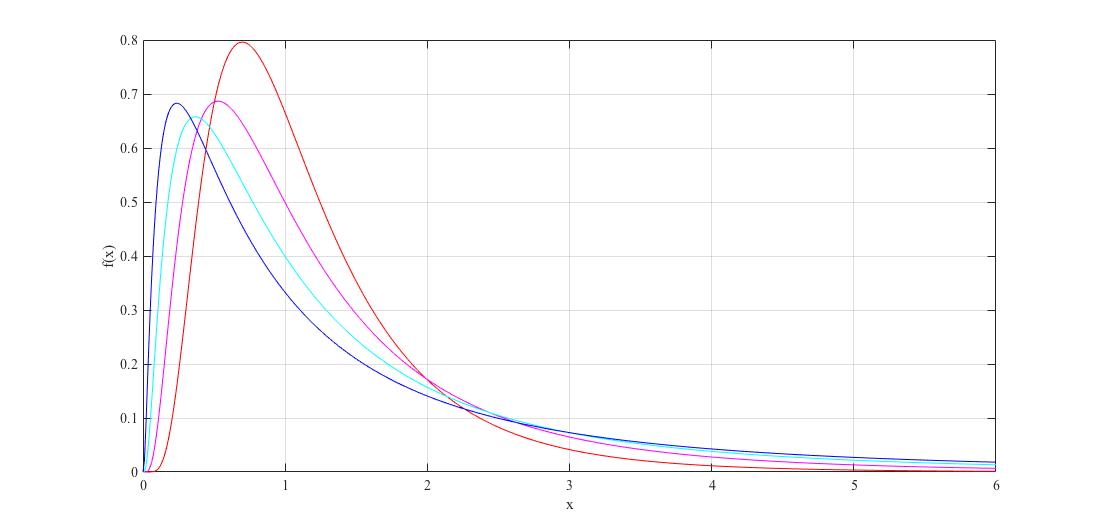
Figure 2: The log-normal density functions with different parameter values: $(\mu=0,\,\sigma=0.6)$ in red, $(\mu=0,\,\sigma=0.8)$ in magenta, $(\mu=0,\,\sigma=1)$ in light blue, $(\mu=0,\,\sigma=1.2)$ in dark blue. Evidently, as parameter $\mu$ does not affect the skewness, the distribution skews more to the right with greater values of $\sigma$.

References

• [1] K. M. Abadir, The Mean-Median-Mode Inequality: Counterexamples. Econometric Theory 21, 477–482 (2005)
• [2] B. Abdous and R. Theodorescu, Mean, Median, Mode IV Statistica Neerlandica 52(3), 356–359 (1998)
• [3] B. C. Arnold and R. A. Groeneveld, Measuring skewness with respect to the mode The American Statistician, 49(1), 34–38 (1995)
• [4] F. Barbaresco, Information geometry of covariance matrix: Cartan-Siegel homogeneous bounded domains, Mostow/Berger fibration and Frechet median In Matrix information geometry Springer, Berlin, Heidelberg, 199–255 (2013)
• [5] S. W. Dharmadhikari and K. Joag-dev, Mean, Median, Mode III Statistica Neerlandica 37(4), 165–168 (1983)
• [6] S. W. Dharmadhikari and K. Joag-dev, Unimodality, Convexity, and Applications Academic Press, New York (1988)
• [7] C. F. Gauss, Theoria Combinationis Observationum Erroribus Minimis Obnoxiae, Pars Prior Commentationes Societatis Regiae Scientiarum Gottingensis Recentiores. 5. (1823)
• [8] F. den Hollander, Probability theory: The coupling method Leiden University, Lectures Notes-Mathematical Institute (2012)
• [9] Y. Kovchegov and P. T. Otto, Path Coupling and Aggregate Path Coupling SpringerBriefs in Probability and Mathematical Statistics, Springer (2018)
• [10] T. M. Liggett Interacting Particle Systems Springer (1985)
• [11] T. Lindvall, Lectures on the coupling method Dover Publications (2002). Originally published in 1992 by John Wiley & Sons, Inc., New York.
• [12] H. L. MacGillivray, Skewness and asymmetry: measures and orderings The Annals of Statistics 14 no.3, 994–1011 (1986).
• [13] A. Müller and D. Stoyan, Comparison methods for stochastic models and risks Vol. 389. Wiley (2002)
• [14] A. Negrón, C. Pertel, and C. Wang, Extensions of True Positive Skewness for Unimodal Distributions Oregon State University Research Experiences for Undergraduates (REU) proceedings (2021) https://sites.science.oregonstate.edu/math_reu/proceedings/REU_Proceedings/Proceedings2021/TeamKovchegov.pdf
• [15] H. Oja, On Location, Scale, Skewness and Kurtosis of Univariate Distributions Scandinavian Journal of Statistics 8(3), 154–168 (1981)
• [16] K. Pearson, Contributions to the Mathematical Theory of Evolution. II. Skew Variation in Homogeneous Material Philosophical Transactions of the Royal Society A: Mathematical, Physical and Engineering Sciences 186, 343–414 (1895)
• [17] J. M. Stoyanov, Counterexamples in probability (3rd ed.) Dover Publications (2014).
• [18] G. Teschl, Ordinary differential equations and dynamical systems Graduate Studies in Mathematics 140, American Mathematical Society, Providence, RI (2012).
• [19] W. R. van Zwet, Convex transformations: a new approach to skewness and kurtosis Statistica Neerlandica 18, 433–441 (1964)
• [20] W. R. van Zwet, Mean, median, mode II Statistica Neerlandica 33(1), 1–5 (1979)