Nonlinear Localized Modes in Two-Dimensional Hexagonally-Packed Magnetic Lattices

Abstract

We conduct an extensive study of nonlinear localized modes (NLMs), which are temporally periodic and spatially localized structures, in a two-dimensional array of repelling magnets. In our experiments, we arrange a lattice in a hexagonal configuration with a light-mass defect, and we harmonically drive the center of the chain with a tunable excitation frequency, amplitude, and angle. We use a damped, driven variant of a vector Fermi–Pasta–Ulam–Tsingou lattice to model our experimental setup. Despite the idealized nature of the model, we obtain good qualitative agreement between theory and experiments for a variety of dynamical behaviors. We find that the spatial decay is direction-dependent and that drive amplitudes along fundamental displacement axes lead to nonlinear resonant peaks in frequency continuations that are similar to those that occur in one-dimensional damped, driven lattices. However, driving along other directions leads to the creation of asymmetric NLMs that bifurcate from the main solution branch, which consists of symmetric NLMs. When we vary the drive amplitude, we observe such behavior both in our experiments and in our simulations. We also demonstrate that solutions that appear to be time-quasi-periodic bifurcate from the branch of symmetric time-periodic NLMs.

I Introduction

Discrete breathers are spatially localized, time-periodic solutions of nonlinear lattice differential equations. They have been studied in a host of scientific areas, including optical waveguide arrays and photorefractive crystals moti , Josephson-junction ladders alex ; alex2 , layered antiferromagnetic crystals lars3 ; lars4 , halide-bridged transition-metal complexes swanson , dynamical models of the DNA double strand Peybi , molecular lattices 2Dreview2015 , Bose–Einstein condensates in optical lattices Morsch , and many others.

Most of the immense volume of work — now spanning more than three decades — on discrete breathers has been in one-dimensional (1D) lattices Flach2007 ; pgk:2011 ; Dmitriev_2016 . Most relevant to the present article is research on discrete breathers in Fermi–Pasta–Ulam–Tsingou (FPUT) lattices, which have nonlinear inter-site coupling FPU55 ; FPUreview . Moreover, FPUT-like lattices with power-law potentials have been used to model a variety of mechanical systems, such as granular crystals Nester2001 ; granularBook ; yuli_book ; gc_review and (more recently) magnetic lattices moleron ; Mehrem2017 ; Marc2017 .

There have also been some studies of breathers in two-dimensional (2D) lattices, although there are many fewer such studies than of 1D lattices. Example physical settings in 2D include crystal lattices Marin2000 ; Dmitriev_2016 , electric circuits English2013 , and dusty plasmas DustyPlasma ; Koukouloyannis2010 . Breathers in 2D lattices have been analyzed with both asymptotic methods Wattis_2Dreview and numerical methods in both homogeneous Flach2D_1997 ; Marin98 and heterogeneous media Qiang2009 ; Koukouloyannis2009 . See 2Dreview2007 ; 2Dreview2015 for overviews of results about 2D breathers.

The 2D setting of the present work is a mechanical system in which each magnet has two displacement fields, which distinguishes it from many studies of scalar 2D lattices, such as those that describe electrical circuits English2013 . Specifically, we examine a lattice of repelling magnets that are arranged in a hexagonal configuration. The choice of a hexagonal arrangement is motivated by the experimental setup, as hexagonal configurations are more robust structurally than other arrangements (such as square ones). At the center of the lattice is a light-mass defect, which introduces a localized defect mode into the spectrum of the linearization of the system. To excite the system experimentally, we drive the center of the lattice by a force that results from the current that flows along a wire that we suspend above the lattice. We model damping using a dashpot term. Putting everything together, the proposed model for the experimental setup is a damped, driven variant of a vector FPUT lattice.

Although a breather is defined as a spatially localized and time-periodic structure, it is useful to label different types of breathers. Linear systems with an impurity or a defect (e.g., with a particle of lighter mass than the other particles) have isolated points in their spectra that lie above the spectral edge. These modes are called “defect localized modes” Mara . In the presence of nonlinearity, breathers can bifurcate from these modes and can exist for frequencies other than the linear defect frequency. Breathers that manifest in this way are called “nonlinear localized modes” (NLMs) Theocharis2009 and are the subject of the present work. By contrast, breathers that do not manifest via a defect or an impurity are called “intrinsic localized modes” (ILMs). One way for ILMs, which we do not investigate in the present paper, to manifest themselves is via a modulation instability of plane waves Flach2007 . In addition to breathers, other kinds of orbits — such as quasiperiodic and chaotic ones — can also occur in nonlinear lattices. For example, such orbits have been identified in strongly nonlinear damped, driven granular chains Nature11 ; hooge12 , suggesting that such solutions may also be present in damped, driven magnetic lattices. In the present work, we examine such NLM states, their stability, and the modes that arise as a result of instabilities.

Our paper proceeds as follows. We present our experimental setup in Sec. II, and we detail the corresponding model equations, linear theory, and numerical methods in Sec. III. We give the main numerical and experimental results in Sec. IV, where we explore NLM profiles, spatial decay, parameter continuations, and nearly time-quasiperiodic orbits. We conclude and discuss future challenges in Sec. V.

II Experimental Setup

(a)

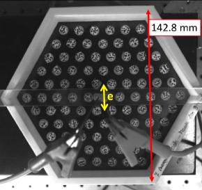
(b)

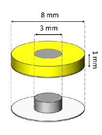
(c)

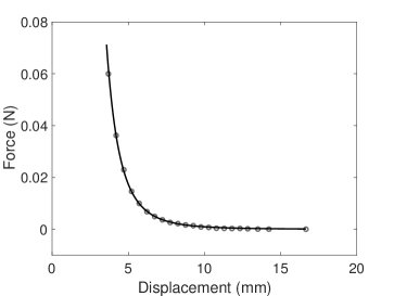
Figure 1: (a) Picture (from a video frame that was used for particle motion tracking) of the experimental setup. The yellow arrow indicates the direction of the external excitation. (b) Sketches of the (top) normal and (bottom) defect particles. (c) Magnetic dipole–dipole interactions in experiments (open grey circles) and fitted model using Eq. (2) (solid black curve).

We place a 2D lattice on an air-bearing table to make the magnetic particles (which constitute the nodes of the lattice) levitate. The lattice consists of 127 magnetic particles that are hexagonally packed. We glue 36 of these particles to the boundaries, and 91 of them are free to move [see Fig. 1(a)]. Each particle is a 3D-printed disc with a hole in the center, where we attach a neodymium magnetic cylinder. We glue a thin piece of cover glass at the bottom to make the surface smoother and thereby improve the levitation of the particles. We build the defect particle, which is located in the center of the lattice, by directly attaching the magnet on the glass without the 3D-printed structure. This particle has a lighter mass and serves as a defect [see Fig. 1(b)]. The mean mass of a normal disc particle is 138.2 mg $\pm$ 3.1 mg (where we measure the standard deviation from a sample of $20$ particles). The defect particle has a mass of 81.6 mg, which corresponds to 58.68% of the normal particle mass.

We excite the defect particle using an external magnetic field that we generate using a conductive wire that we place over the particle at a height of $3$ mm. We generate the AC current that flows through the wire from a Lock-In amplifier (SR860 500kHz DSP Lock-in Amplifier), and we amplify it with an audio amplifier (Topping TP22, class D). The equation that describes the force that the wire exerts on a magnet at distance $r$ from it can be calculated as:

$$F_{\rm wire}(r)=\frac{I\mu_{0}\mathcal{M}}{2\pi}\frac{h^{2}-r^{2}}{(h^{2}+r^{2})^{2}}\,,$$ (1)

where $h$ is the height of the wire from the plane of floating discs, $I$ is the wire current, $\mu_{0}=4\pi\cdot 10^{-7}$ N A^-2 is the magnetic permeability, and $\mathcal{M}=7.8\cdot 10^{-3}$ Am² is the magnetic moment of the floating disc. See the appendix for the derivation of Eq. (1). We use harmonic excitations in our experiment, so the current through the wire is $I(t)=aI_{0}\sin(2\pi ft)$, where $f$ is the drive frequency (in Hz), $a$ is the drive-voltage amplitude (in Volts), and $I_{0}=0.1$ A V^-1 is the current per unit voltage that we measure in the wire.

The magnets repel each other. In the ideal situation of a perfect dipole–dipole interaction, the magnetic force between two repelling magnets is

$$F_{\mathrm{magnet}}(r)=Ar^{p}\,,$$ (2)

where $r$ is the distance (in meters) between the two center points of the magnets, $p=-4$, and $A=3\mu_{0}\mathcal{M}^{2}/2\pi$. Although Eq. (2) is reasonable for large separation distances, we obtain better agreement by empirically determining $A$ and $p$. Because the force between two magnetic dipoles is too small to measure directly, we create a pair of plastic plates, with 25 magnets attached to each plate. We position the plates to align each pair of cylindrical magnets from opposite plates through their radial directions. We measure the repulsive force as a function of the displacement between these two plates in a materials tester (Instron ElectroPuls E3000). The distance between the magnets on each plate is large enough (specifically, it is 2.5 cm) so that we can neglect interactions between magnets that are not aligned. The distance between a magnet on the first plate and the non-aligned magnets of the other plate is larger than 25 mm. As one can see in Fig. 1(c) the interaction force already tends to $0$ for distances smaller that are significantly smaller than 25 mm. Consequently, the measured force is approximately equal to the sum of the repulsive force of the 25 isolated magnet pairs. We fit the data using Eq. (2), which yields $p\approx-4.2$ and $A\approx 3.8\cdot 10^{-12}N/m\textsuperscript{$p$}$ [see Fig. 1(c)].

We monitor the motion of the central particle using a laser vibrometer (Polytec CLV-2534), and we record the remainder of the lattice using a digital camera (Point Grey GS3-U3-41C6C-C) with a frame rate of 90 fps. We analyze the images using digital-image-correlation (DIC) software (VIC-2D) to determine each particle’s velocity. We inspect half of the lattice, as the cables that are connected to the driving wire block most of the system’s other half [see Fig. 1(a)]. Due to imperfections at the bottom of the glass disks (e.g., dust, scratches, and so on) and the fact that mass is not distributed evenly on a disk, a few particles start to rotate when they are levitated by the air that flows out of the air-bearing table. The image correlation software then loses track of them. We ignore these rotating discs in our subsequent analysis. To estimate the value of the damping coefficient, we excite the center particle and record the resulting temporal amplitude decay once we switch off the excitation. We fit the decay to an exponential function, which we then use to calculate the damping coefficient $\gamma\approx 10.52\cdot 10^{-3}$N s/m. The lattice particles are always in motion with at least small speeds, even in the absence of excitation. This is due to interactions with the air flow from the table and to imperfections (e.g., nonaxisymmetric mass distributions) of the particles. We use this motion to estimate the noise in the system. To evaluate the amount of noise, we record the lattice motion without excitation as a comparison. We summarize the values of the parameters in Table 1.

Table 1: Summary of the parameter values in our experimental setup.

Description	Symbol	Value (measured)	Description	Symbol	Value (fitted)
Mass of bulk magnet	$M_{b}$	$138.2$ mg	Magnetic coefficient	$A$	$3.8\cdot 10^{-12}$ N/m$p$
Defect mass	$M_{\delta}$	$81.6$ mg	Nonlinearity	$p$	$-4.2$
Equilibrium distance	$\delta$	$13.7$ mm	Damping coefficient	$\gamma$	$10.52\cdot 10^{-3}$N s/m
Wire height	$h$	$3$ mm	Magnetic moment	$\mathcal{M}$	$7.8\cdot 10^{-3}$ A m2

III Theoretical Setup

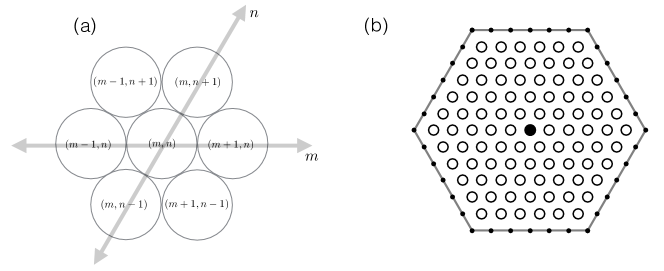
Figure 2: (a) Orientation for our convention of indexing particles in a hexagonal lattice. The $m$ axis and $n$ axis meet at an angle of $\theta=\pi/3$. (b) A hexagonal lattice with $w=6$ magnets along each edge of the lattice. The empty circles and solid center circle represent the locations of the magnets in equilibrium. When in equilibrium, the center-to-center distance between any two adjacent magnets is $\delta$. The outer hexagonal boundary is the solid gray hexagon that encloses the lattice. On the boundary, the solid points represent fixed (i.e., immovable) magnets. There are $w+1$ such magnets along each edge of the boundary. The solid circle represents the defect particle, which has index $(m,n)=(0,0)$.

III.1 Model Equations

Our goal is to study NLMs in a 2D hexagonal lattice. In selecting equations to model the system that we described in Sec. II, we seek the simplest possible model that incorporates the ingredients (nonlinearity, discreteness, and dimensionality) that are essential for NLMs and also yield reasonable agreement with experimental data. It is in this spirit that we develop our model equations. After doing so (at the end of this section), we briefly discuss model simplifications.

We consider a hexagonally packed lattice of magnets. We use the lattice basis vectors $e_{1}=(1,0)$ and $e_{2}=(1/2,\sqrt{3}/2)$. Let $\mathbf{q}_{m,n}(t)=(x_{m,n}(t),y_{m,n}(t))\in{\mathbb{R}}^{2}$ denote the displacement from the static equilibrium of the magnet at position $\textbf{p}=\delta(me_{1}+ne_{2})$ in the plane [see Fig. 2(a)], where $\delta$ is the center-to-center distance between two particles at equilibrium. The lattice indices $m$ and $n$ take the values $m,n\in\{-w,-(w-1),\ldots,0,\ldots,w-1,w\}$, where $w$ is the number of magnets along an edge of the hexagon. The lattice boundary is given by the hexagon with magnets at positions $(w\delta\cos(j\pi/3),w\delta\sin(j\pi/3))$, where $j=0,1,\ldots,w-1$ [see Fig. 2(b)]. For our fixed boundary conditions along the edge of the hexagonal boundary, $\mathbf{q}_{m,n}(t)=0$ if $|m+n|>w$.

One can express the distance between the magnet with index $(m,n)$ and one of its nearest neighbors in terms of the displacements $x_{m,n}$ and $y_{m,n}$ of the magnets from their respective equilibrium positions. Once we determine the distance, we compute the resulting force using Eq. (2). Summing the forces from each of the six nearest neighbors and applying Newton’s second law leads to the following equations of motion:

$$\begin{array}[]{ll}\displaystyle M_{m,n}\ddot{\mathbf{q}}_{m,n}=&-\mathbf{F}_{0}(\mathbf{q}_{m+1,n}-\mathbf{q}_{m,n})-\mathbf{F}_{1}(\mathbf{q}_{m,n+1}-\mathbf{q}_{m,n})+\mathbf{F}_{-1}(\mathbf{q}_{m,n}-\mathbf{q}_{m-1,n+1})\\ &+\mathbf{F}_{0}(\mathbf{q}_{m,n}-\mathbf{q}_{m-1,n})+\mathbf{F}_{1}(\mathbf{q}_{m,n}-\mathbf{q}_{m,n-1})-\mathbf{F}_{-1}(\mathbf{q}_{m+1,n-1}-\mathbf{q}_{m,n})-\gamma\dot{\mathbf{q}}_{m,n}+\mathbf{F}^{\mathrm{ext}}_{m,n}(t)\,.\end{array}$$ (3)

The vector functions $\mathbf{F}_{j}(\mathbf{q})=\mathbf{F}_{j}(x,y)\in{\mathbb{R}}^{2}$ have a magnitude of

$$|\mathbf{F}_{j}(x,y)|=A\left[\sqrt{(\delta\cos(\theta_{j})+x)^{2}+(\delta\sin(\theta_{j})+y)^{2}}\,\right]^{p}\,,\quad\theta_{j}=\frac{j\pi}{3}\,,\quad j\in\{-1,0,1\}\,.$$

The mass of the magnet with index $(m,n)$ is $M_{m,n}$. The dashpot $\gamma\dot{\mathbf{q}}_{m,n}$ is a phenomenological term that we add to account for damping. Using such a term has yielded reasonable agreement with experiments in other, similar lattices moleron ; cantilevers ; magBreathers . The quantity $\mathbf{F}^{\mathrm{ext}}_{m,n}$ is the external force that we apply to the magnet at $(m,n)$. In the present article, we consider excitations via a wire that is directly above the center of the lattice. The magnitude of the excitation is given by Eq. (1). Therefore,

$$\mathbf{F}^{\mathrm{ext}}_{0,0}(t)=\ \ a\sin(2\pi ft)\,\frac{I_{0}\mu_{0}\mathcal{M}}{2\pi}\begin{pmatrix}\cos(\phi)\frac{h^{2}-x_{0,0}^{2}}{(h^{2}+x_{0,0}^{2})^{2}}\\ \sin(\phi)\frac{h^{2}-y_{0,0}^{2}}{(h^{2}+y_{0,0}^{2})^{2}}\end{pmatrix}\,,$$ (4)

where $\phi$ is the angle of the excitation and $\mathbf{F}^{\mathrm{ext}}_{m,n}=0$ when $m\neq 0$ and $n\neq 0$. In our experiments and in most of our numerical computations, the excitation angle is $\phi=\pi/2$, so we excite only the $y$-component of the center magnet. We will also explore some other excitation angles. As we discuss in the appendix, the lattice forces dominate the dynamics. The wire has only a small effect on magnets that are beyond the center of the lattice. For example, at equilibrium, the force that is exerted on the center magnet by the wire is two orders of magnitude larger than the force that the wire exerts on the center magnet’s nearest neighbors. Compare Eq. (1) with $r=0$ and $r=\delta$.

In our model, we ignore effects beyond nearest-neighbor coupling of the magnetic interactions. It is known that such long-range effects can alter the structure of localized modes. For example, it was shown in Flach_long that the spatial decay of breathers can transition from exponential spatial decay to algebraic decay in lattices with algebraically decaying interaction forces (as is the case in our model) for lattices with sufficiently many sites. More recently, Molerón et al. magBreathers studied NLMs in a 1D magnetic lattice using a model with long-range interactions. Although the differences between long-range and nearest-neighbor lattices that were considered in magBreathers are detectable, they are still small. For example, at equilibrium, the force that is exerted on the center magnet by its nearest neighbors is one order of magnitude larger than that exerted by its next-nearest neighbor. (Compare Eq. (2) with $r=\delta$ and $r=2\delta$.) Therefore, to keep our model as simple as possible, we ignore such small long-range effects.

In our analysis of experimental data we ignore magnets that are rotating, so our model does not account for rotation. This leaves air resistance as the primary source of damping. Given the size of the magnets and velocities that we consider, we employ a linear dashpot SteidelBook . We also assume that the magnets stay in a plane. We validate the many assumptions that we have made in formulating the model in Eq. (3) via a direct comparison with experimental results in Sec. IV.

For the remainder of the manuscript, we fix all parameters of the model (and we summarize them in Table 1), except for the excitation amplitude $a$, frequency $f$, and angle $\phi$. We will specify these in our various examples. In all cases, we examine a lattice with a single defect particle in the center and a hexagonal boundary with a length of $w=6$ magnets (see Fig. 2). Importantly, we do not fit the parameter values to the reported experimental results. Instead, we determine them beforehand using the procedures that we detailed in Sec. II.

III.2 Linear Analysis

(a)

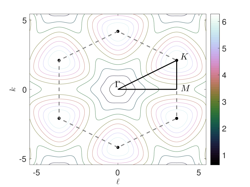
(b)

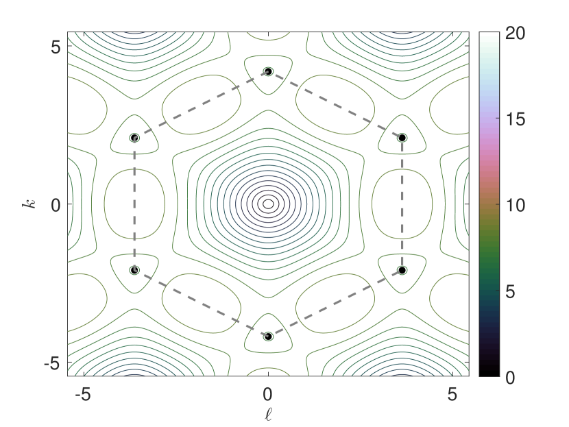
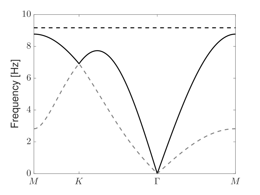
(c)

Figure 3: (Color Online) (a) Contour plot of the bottom dispersion surface. We show the irreducible Brillouin zone as the triangle with magnets at the points that we mark by $\mathbf{M}$, $\mathbf{K}$, and $\mathbf{\Gamma}$. (b) Contour plot of top dispersion surface. (c) Band structure along the edge of the irreducible Brillouin zone [also see the triangle in panel (a)] for the bottom (dashed gray curve) and top (solid black curve) dispersion surfaces. The horizontal dashed curve corresponds to the defect-mode frequency $f\approx 9.17$ Hz in a finite-dimensional system with a mass ratio of $M_{\delta}/M_{b}\approx 0.5868$, where $M_{\delta}$ denotes the mass of the defect magnet and $M_{b}$ denotes the mass of the other (“bulk”) magnets.

We start with the basic linear theory of localized modes for our hexagonal magnetic lattice. We are particularly interested in modes with frequencies that lie above the cutoff frequency of the pass band. We first derive an analytical expression for the cutoff frequency, which is straightforward for an infinite-dimensional Hamiltonian system (i.e., with all integers $m$ and $n$, along with $a=0$ and $\gamma=0$). We then numerically estimate the frequency of a linear mode that is associated with the defect for in the finite-dimensional Hamiltonian system. Finally, we compute linear localized modes in the associated finite-dimensional damped, driven system.

Assuming small strains, such that

$$\frac{|\mathbf{q}_{m\pm 1,n}-\mathbf{q}_{m,n}|}{\delta}\ll 1\,,\quad\frac{|\mathbf{q}_{m,n\pm 1}-\mathbf{q}_{m,n}|}{\delta}\ll 1\,,\quad\frac{|\mathbf{q}_{m\pm 1,n\mp 1}-\mathbf{q}_{m,n}|}{\delta}\ll 1\,,$$ (5)

one can Taylor expand,

$$\mathbf{F}_{j}(\mathbf{q})\approx\mathbf{F}_{j}(\mathbf{q}_{0})+D\mathbf{F}_{j}(\mathbf{q}_{0})\mathbf{q}\,,$$

where $D\mathbf{F}_{j}$ is the Jacobian matrix of $\mathbf{F}_{j}$. Using this notation, we write the linearized equations of motion:

$$M_{m,n}\ddot{\mathbf{q}}_{m,n} =-D\mathbf{F}_{0}(\mathbf{q}_{m+1,n}+\mathbf{q}_{m-1,n})-D\mathbf{F}_{1}(\mathbf{q}_{m,n+1}+\mathbf{q}_{m,n-1})$$

$$\quad-D\mathbf{F}_{-1}(\mathbf{q}_{m-1,n+1}+\mathbf{q}_{m+1,n-1})+2(D\mathbf{F}_{0}+D\mathbf{F}_{1}+D\mathbf{F}_{-1})\mathbf{q}_{m,n}\,,$$ (6)

where the entries of the Jacobian matrices are denoted by,

$$D\mathbf{F}_{j}=\begin{pmatrix}a_{j}&b_{j}\\ c_{j}&d_{j}\end{pmatrix}\,,\qquad j\in\{-1,0,1\}\,,$$

with

$$a_{-1}=p\hat{\delta}\,, b_{-1} =0\,, c_{-1} =0\,, d_{-1} =\hat{\delta}\,,$$

$$a_{0}=\frac{3+p}{4}\hat{\delta}\,, b_{0} =\frac{\sqrt{3}(p-1)}{4}\hat{\delta}\,, c_{0} =b_{0}\,, d_{0} =\frac{1+3p}{4}\hat{\delta}\,,$$

$$a_{1}=a_{0}\,, b_{1} =-b_{0}\,, c_{1} =-c_{0}\,, d_{1} =d_{0}\,,$$

where $\hat{\delta}\equiv A\delta^{p-1}$. For a monoatomic system (in which all magnets are identical, such that $M_{m,n}=M_{b}$), the linear system has plane-wave solutions

$$\mathbf{q}_{m,n}=\mathbf{q}_{0}\exp\left(i(km+\frac{n}{2}(k+\sqrt{3}\ell))\right)e^{i\omega t}\,,\quad\mathbf{q}_{0}\in{\mathbb{C}}^{2}\,,\quad k,\ell,\omega\in{\mathbb{R}}\,,$$

where the wavenumbers $k,\ell$ and angular frequency $\omega=\omega(k,\ell)$ satisfy the dispersion relationship

$$\left[\omega(k,\ell)\right]^{2}=\frac{\omega_{a}+\omega_{d}\pm\sqrt{\rule{0.0pt}{11.38092pt}(\omega_{a}+\omega_{d})^{2}-4(\omega_{a}\omega_{d}-\omega_{b}\omega_{c})}}{2}\,,$$ (7)

where

$$\omega_{\alpha}(k,\ell)=(-2\alpha_{-1}\cos(k)-2\alpha_{0}\cos(k/2+\sqrt{3}/2\ell)-2\alpha_{1}\cos(k/2-\sqrt{3}/2\ell)+2(\alpha_{-1}+\alpha_{0}+\alpha_{1}))/M_{b}$$

and $\alpha\in\{a,b,c,d\}$. In Fig. 3(a,b), we show contour plots of the two dispersion surfaces from Eq. (7). The dispersion curves along the edge of the irreducible Brillouin zone are shown in Fig. 3(c). The cutoff value of the pass band has the wavenumber pair $(k,\ell)=(0,2\pi/3)$, which is where the dispersion curve attains its maximum value. For the parameter values in Table 1, the cutoff frequency is $f_{c}=\omega(0,2\pi/3)_{+}/(2\pi)\approx 8.77$ Hz, where $\omega_{+}$ corresponds to the top dispersion surface.

The presence of the lighter defect introduces a linear mode into the system that is localized in space and oscillates with a frequency above the cutoff frequency of the linear monoatomic system. With the light-mass defect at the center of the lattice, we write

$$M_{m,n}=\left\{\begin{array}[]{ l l }{M_{\delta}\,,}&{n=0\,\text{ and }\,m=0}\\ {M_{b}\,,}&{\text{ otherwise}\,,}\end{array}\right.$$ (8)

where $(0,0)$ is the index of the mass defect with mass $M_{\delta}$, the quantity $M_{b}$ is the mass of a magnet in the “bulk” (i.e., the non-defect mass), and $M_{\delta}<M_{b}$. We numerically compute the linear modes of the system with a mass defect, and we are thereby able to consider finite lattices. We use a hexagonal boundary with edge length $w=6$ magnets [see Fig. 2(b)]. One can embed this lattice into a square matrix of size $N\times N$, where $N=2w-1$ is the number magnets along the $n=0$ line of the lattice. Let $X(t)$ be the $N\times N$ matrix whose $(m,n)$th entry is $x_{m,n}(t)$, and let $Y(t)$ be the $N\times N$ matrix whose $(m,n)$th entry is $y_{m,n}(t)$. We enforce the fixed hexagonal boundaries by setting the displacements of magnets with indices $(m,n)$ such that $|m+n|>w$ to $0$. We define the $N\times N$ matrix operators $L_{\alpha}$ through

$$L_{\alpha}Y=\alpha_{1}DY+\alpha_{2}YD+\alpha_{3}(E^{T}YE^{T}+EYE-2Y)\,,$$ (9)

where $\alpha\in\{a,b,c,d\}$; the $N\times N$ tridiagonal matrix $D$ has $1$ entries on the super-diagonals and sub-diagonals, $2$ entries along the diagonal, and $0$ entries everywhere else; $E$ is an $N\times N$ matrix with $1$ entries along the super-diagonal and $0$ entries everywhere else; and $E^{T}$ is the transpose of $E$. With these definitions, Eq. (III.2) becomes

$$M\circ\ddot{X}(t)=L_{a}X(t)+L_{b}Y(t)\,,$$

$$M\circ\ddot{Y}(t)=L_{c}X(t)+L_{d}Y(t)\,,$$ (10)

where $M$ is an $N\times N$ matrix in which all entries except the $(0,0)$ entry (which is equal to $M_{\delta}$) are equal to $M_{b}$. The operation $\circ$ denotes pointwise multiplication (i.e., the Hadamard product). The system (III.2) has solutions of the form $X(t)=\tilde{X}e^{i\omega t}$ and $Y(t)=\tilde{Y}e^{i\omega t}$, where $\tilde{X}$ and $\tilde{Y}$ are $N\times N$ time-independent matrices and

$$-\omega^{2}\begin{pmatrix}M\circ\tilde{X}\\ M\circ\tilde{Y}\end{pmatrix}=\begin{pmatrix}L_{a}&L_{b}\\ L_{c}&L_{d}\end{pmatrix}\begin{pmatrix}\tilde{X}\\ \tilde{Y}\end{pmatrix}\,.$$ (11)

One can cast Eq. (11) as a standard eigenvalue problem by letting $\lambda=-\omega^{2}$ and unwrapping the $\tilde{X}$ and $\tilde{Y}$ matrices into equivalent row vectors and reshaping the block matrix (with entries given by $L_{\alpha}$) into a corresponding $2N^{2}\times 2N^{2}$ matrix. One can then numerically solve the resulting eigenvalue problem to obtain $2N^{2}$ eigenvalues and their corresponding modes. Using the values in Table 1 and $w=6$ (which yields $N=11$), we see that two eigenvalues (each with a frequency of $\sqrt{-\lambda}/(2\pi)=\omega/(2\pi)=f_{d}\approx 9.17$) lie above the cutoff frequency $f_{c}\approx 8.77$ Hz. We plot the value of $f_{d}$ as the horizontal dashed line in Fig. 3(c), and we show the two corresponding modes in Fig. 4(a,b). Both of these modes are spatially localized, as desired.

Now suppose that there is driving and damping. Near the background state, equations (III.2) yield the following approximate system:

$$M\circ\ddot{X}(t) =L_{a}X(t)+L_{b}Y(t)-\gamma\dot{X}(t)+a\mathcal{A}\cos(\phi)\sin(2\pi ft)\,,$$ (12)

$$M\circ\ddot{Y}(t) =L_{c}X(t)+L_{d}Y(t)-\gamma\dot{Y}(t)+a\mathcal{A}\sin(\phi)\sin(2\pi ft)\,,$$ (13)

where $\mathcal{A}$ is an $N\times N$ matrix that has all $0$ entries except for the single nonzero entry

$$\mathcal{A}_{0,0}=\frac{I_{0}\mu_{0}\mathcal{M}}{2\pi h^{2}}\,.$$

We obtain $\mathcal{A}$ by expanding the external drive function $\mathbf{F}^{\mathrm{ext}}$ near the vanishing displacements and maintaining the leading, non-vanishing term. We can then find solutions of the system (12,13) in the form

$$X(t)=\tilde{X}_{1}\cos(2\pi ft)+\tilde{X}_{2}\sin(2\pi ft)\,,\quad Y(t)=\tilde{Y}_{1}\cos(2\pi ft)+\tilde{Y}_{2}\sin(2\pi ft)\,,$$ (14)

where we obtain the $N\times N$ matrices $\tilde{X}_{1}$, $\tilde{X}_{2}$, $\tilde{Y}_{1}$, and $\tilde{Y}_{2}$ by substituting Eq. (14) into Eqs. (12) and (13) and then solving the resulting system of linear equations.

We use root mean square (RMS) quantities as our principal diagnostic for evaluating our results, such as in our bifurcation diagrams. Most commonly, we compute the RMS of the velocity of the $y$-component of the center particle (i.e., $\dot{y}_{0,0}$). In this case,

$$\mathrm{RMS}=\sqrt{\frac{\int_{0}^{T}\dot{y}_{0,0}^{2}(t)\,dt}{T}}\,,$$

where $T=1/f$ is the period of the excitation frequency. We show a plot of the RMS of the linear state (14) in Fig. 4(c) as a function of the excitation frequency for a fixed amplitude of $a=0.01$ mV and an excitation angle of $\phi=\pi/2$. The lone resonant peak above the cutoff point is close to the estimated defect frequency $f_{d}\approx 9.17$ Hz.

In Fig. 4(d), we show a frequency sweep in our experiment for $a=4$ mV and $\phi=\pi/2$. We show the theoretical values of the cutoff frequency $f_{c}\approx 8.77$ Hz and defect frequency $f_{d}\approx 9.17$ Hz that we found in Sec. III.2 as vertical solid and dashed lines, respectively. We observe that the experimental resonant peak is close to the theoretical value. To obtain a cleaner resonant peak, we use an excitation amplitude that is large enough to overcome the noise of the system. One such amplitude is $a=4$ mV. As we will see in Sec. IV, an excitation amplitude of $a=4$ mV is already in the nonlinear regime of the system.

(a)

(b)

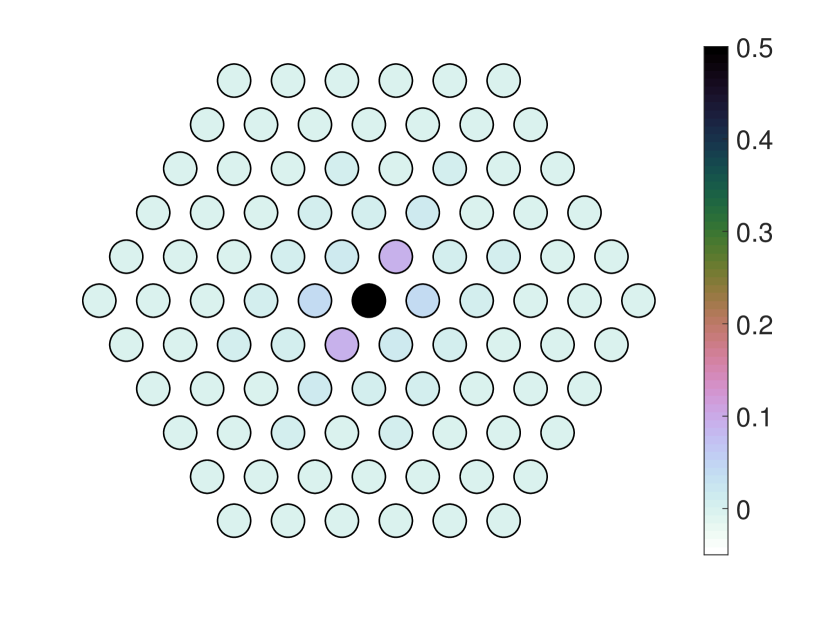
(c)

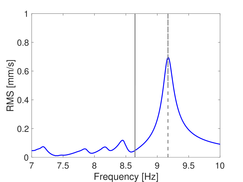
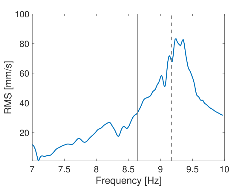
(d)

Figure 4: (a,b) Shape of the two modes with defect frequency $f_{d}\approx 9.17$ Hz of the linear Hamiltonian system (III.2) with $w=6$ magnets along each edge of the boundary. The color intensity at each point $(m,n)$ corresponds to $\sqrt{\dot{x}_{m,n}^{2}+\dot{y}_{m,n}^{2}}$. (c) RMS of $\dot{y}_{0,0}$ of the linear damped, driven solution (14) as a function of the drive frequency $f$ with excitation amplitude $a=0.01$ mV and $\phi=\pi/2$. (d) RMS of the velocity of the center particle of the experimental frequency sweep with $a=4$ mV and $\phi=\pi/2$.

III.3 Numerical Methods for the Computation of Nonlinear Localized Modes and Their Stability

For the remainder of our paper, we focus on how the presence of nonlinearity affects the “defect-induced” linear localized modes of the system [see, e.g., Fig. 4(c)]. We refer to these solutions, which are localized in space and periodic in time, as nonlinear localized modes (NLMs). Unlike in the linear equations, we are unable to obtain analytical solutions for NLMs using the ansatz (14). Therefore, we turn to numerical computations. We compute time-periodic orbits of Eq. (3) with period $T=1/f$ to high precision by finding roots of the map $G=\mathbf{x}(T)-\mathbf{x}(0)$, where $\mathbf{x}(T)$ is the solution of Eq. (3) at time $T$ with initial condition $\mathbf{x}(0)$. Additionally, $\mathbf{x}\in{\mathbb{R}}^{4N^{2}}$ is the vector that results from reshaping the matrix with elements $x_{m,n}$, $y_{m,n}$, $\dot{x}_{m,n}$, and $\dot{y}_{m,n}$ into row vectors and concatenating them into a single vector. We obtain roots of the map $G$ using a Jacobian-free Newton–Krylov method nsoli with an initial guess of our linear state (14). We compute bifurcation diagrams using a pseudo-arclength continuation algorithm Doedel with the excitation frequency $f$ or amplitude $a$ as our continuation parameter. Once we obtain the branches of a bifurcation diagram, we determine the linear stability of each solution $\mathbf{x}$ by solving the variational equations $V^{\prime}=DG\cdot V$ with initial condition $V(0)=I$, where $I$ denotes the identity matrix and $DG$ is the $4N^{2}\times 4N^{2}$ Jacobian matrix of the right-hand side of Eq. (3) evaluated at the solution $\mathbf{x}$ HirschSmaleDevaney . We calculate the Floquet multipliers, which are hereafter denoted by $\sigma$, for a solution by computing the eigenvalues of the matrix $V(T)$. If all of the Floquet multipliers of a solution have an absolute value that is less than or equal to $1$, we say that the solution is “linearly stable”. Otherwise, we say that the solution is “unstable”. Clearly, the Floquet multipliers only give information about the spectral stability of the solutions, and marginal instabilities associated with unit Floquet multipliers and nonlinear instabilities are possible. Therefore, stability is verified through numerical simulations. In our bifurcation diagrams, solid blue segments correspond to stable parameter regions and dashed red segments correspond to unstable regions. We compute the Floquet multipliers after we obtain a solution with the Newton–Krylov method to avoid repeatedly solving the large variational system. This computation would be necessary if we were using a standard Newton method, because the Jacobian of the map $G$ is $V(T)-I$.

IV Main Results

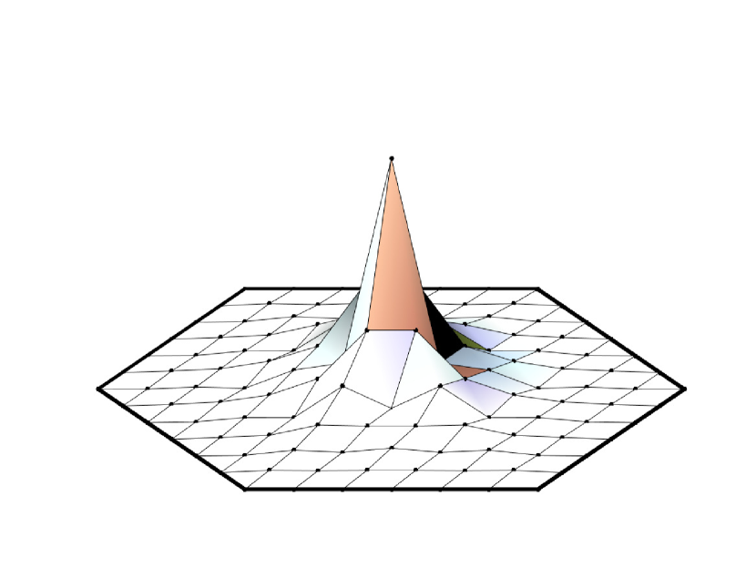
(a)

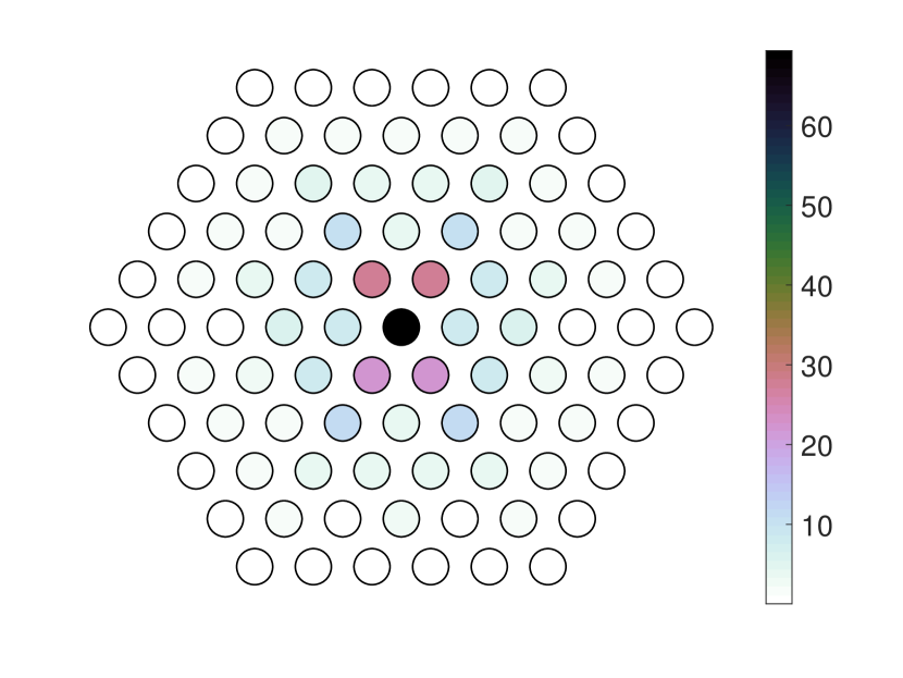
(b)

(c)

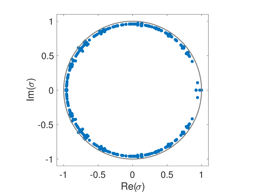
(d)

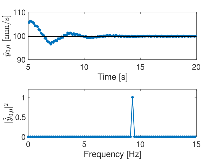
Figure 5: Nonlinear localized mode of Eq. (3) that we obtain using a Newton–Krylov method for $a=4$ mV, $\phi=\pi/2$, and $f=9.3$ Hz. (a) A surface plot of the NLM. We show the RMS velocity of each magnet in the lattice. (b) Intensity plot of the NLM, where the color intensity corresponds to the RMS. (c) Floquet multipliers $\sigma$ (blue marks) that are associated with the NLM in the complex plane. We show the unit circle in gray. All multipliers lie within (or on) the unit circle, indicating that this solution is stable. (d) In the top panel, we show local maxima of the time series of $\dot{y}_{0,0}$ when evolving zero initial data (i.e., the initial values of all variables are equal to $0$) for $a=4$ mV, $\phi=\pi/2$, and $f=9.3$ Hz. We approach the value $\dot{y}_{0,0}\approx 99.8$ mm/s of the stable NLM. (See the black line.) In the bottom panel, we show the Fourier transform of the final $5$ seconds of the time series of $\dot{y}_{0,0}$. This reveals a single large peak at frequency $f\approx 9.3$ Hz.

IV.1 Numerical NLMs

Using the Newton–Krylov method that we described in Sec. III.3, we obtain a time-periodic solution with $f=9.3$ Hz, $a=4$ mV , and $\phi=\pi/2$. Additionally, because $f=9.3>8.77\approx f_{c}$, this solution is localized in space [see Fig. 5(a)]. The dominant peak is at the center of the lattice and the next-largest amplitudes are for the magnets that are adjacent to the center magnet at angles $\pi/3$, $2\pi/3$, $4\pi/3$, and $5\pi/3$ [see Fig. 5(b)]. This is not surprising, because we are exciting the lattice along the $\phi=\pi/2$ direction. The Floquet multipliers that are associated with this solution each have a magnitude that is no more than $1$, indicating that the solution is stable [see Fig. 5(c)]. Indeed, upon simulating Eq. (3) with initial values of all variables equal to $0$ (i.e., “zero initial data”) and $f=9.3$ Hz, $a=4$ mV , and $\phi=\pi/2$, the dynamics approaches this stable NLM. [See the top panel of Fig. 5(d).] As expected, the Fourier transform of the corresponding time series is localized around a frequency $f\approx 9.3$ Hz.

The spatial decay of the tails of the NLM depends on which direction of observation one considers. For example, if one measures the RMS velocity of the magnets that lie along the $\theta=\pi/3$ direction, the decay appears to be exponential or faster. See the solid blue squares in Fig. 6(a), which shows the RMS velocity versus distance from the origin (following the $\theta=\pi/3$ direction) in a semilog plot for the NLM from Fig. 5 [i.e., for the NLM with $f=9.3$ Hz, $a=4$ mV , and $\phi=\pi/2$]. This is consistent with the spatial decay properties of breathers in continuous-space settings, such as the ones in the quintic Ginzburg–Landau equation that were studied in Boris2Dtail . The tails of the breathers in Boris2Dtail decay at rate $e^{-br}/\sqrt{r}$, where $b>0$ is a constant. The solid yellow circles exhibit a similar decay for the magnets along the $\theta=0$ direction for our solution above, although we observe some modulation in the decay profile, in contrast to the $\theta=\pi/3$ case. Modulations in spatial decay have been studied in other settings, such as in the biharmonic $\phi^{4}$ model modulated2Dtail . We observe similar decay properties for an NLM with $f=9.3$ Hz, $a=5.5$ mV and $\phi=\pi/2$ [see Fig. 6(b)].

IV.2 Experimental NLMs

In our experiments, it is difficult to initialize the system with predetermined positions and velocities. To obtain the NLM, we excite the system with a small amplitude ($a=1$ mV) which we increase gradually to the value $a=4$ mV over about $3$ minutes. Because we predict the NLM to be stable at the resulting parameter values, we record data after 90 periods of motion have elapsed once we attain the value $a=4$ mV. We track the velocities at the center particle with a laser vibrometer (see Sec. II), and we record the time series of the magnet velocities using an oscilloscope. [See the top panel of Fig. 6(c).] As expected, we obtain dynamics that are periodic in time, as we can see not only with the time series but also via its Fourier transform [which we show in the bottom panel of Fig. 6(c)]. We obtain similar experimental results for an amplitude of $a=5.5$ mV.

To examine the spatial decay of the experimental NLM, we record the positions of the magnets in half of the lattice using a digital camera (see Sec. II). By numerically differentiating the positions, we obtain an estimate for the velocities of these magnets. We were unable to do a complete full-field realization, because the DIC loses track of some magnets (if, e.g., the magnets begin to spin). However, we captured enough data to compute the decay along the two primary directions ($\theta=\pi/3$ and $\theta=0$) that we examined in our numerical NLMs. The open blue squares of Fig. 6(a) show the decay along the $\theta=\pi/3$ direction and the open yellow circles show the decay along the $\theta=0$ direction for data that we obtained with $f=9.3$ Hz, $a=4$ mV, and $\phi=\pi/2$. The horizontal dashed line is our estimated mean value of the noise (see Sec. II). We show the experimental decay rates along with our numerical results. Although the numerical values overestimate the RMS velocity, the agreement is still reasonable, especially for the center magnet. We find similar decay properties in our experiment with $f=9.3$ Hz, $a=5.5$ mV , and $\phi=\pi/2$. [See the open markers of Fig. 6(b).]

Recall that we do not tune the numerical results to fit the experimentally obtained NLM solution. Instead, we determine each of the parameter values beforehand, as described in Sec. II.

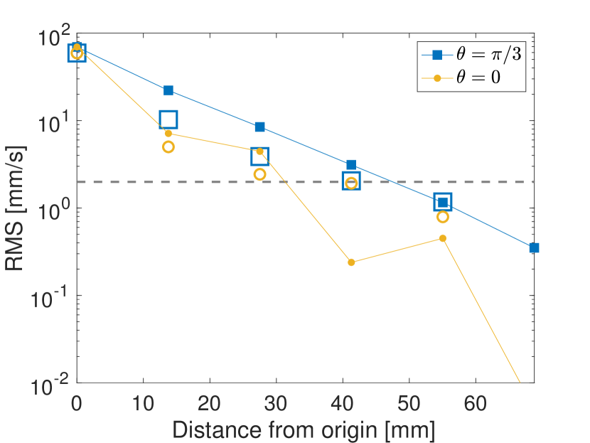
(a)

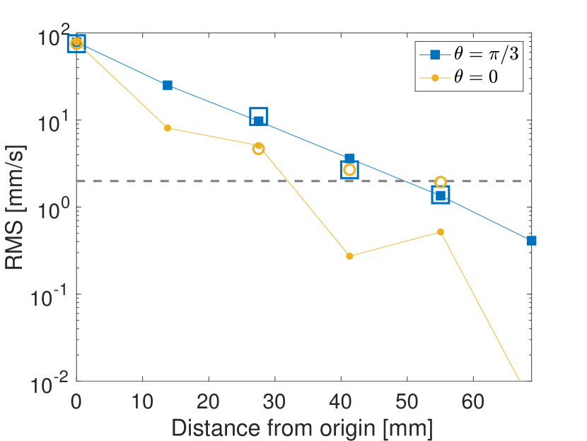
(b)

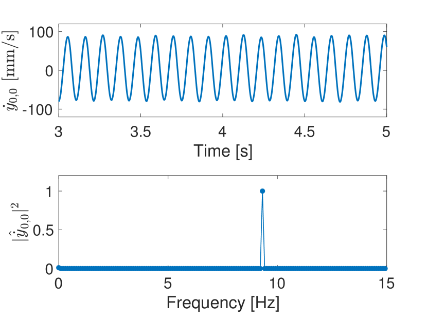
(c)

Figure 6: (a) Decay of the NLM in the $\theta=\pi/3$ (blue squares) and $\theta=0$ (yellow circles) directions for a drive amplitude of $a=4$ mV, drive angle of $\phi=\pi/2$, and drive frequency of $f=9.3$ Hz. We show the RMS velocity versus the distance to the origin of the lattice. We show experimental results as open markers and the numerical results as solid markers that are connected by lines. (b) The same as panel (a), but for a drive amplitude of $a=5.5$ mV. (c) Time series (top panel) of the center particle of the experimental NLM and corresponding Fourier transform (bottom panel) with $\phi=\pi/2$, $f=9.3$ Hz, and $a=4$ mV. Despite the presence of some noise, the solution is predominantly periodic in time. Indeed, the Fourier transform of the time signal is highly localized around the frequency $f=9.3$ Hz.

IV.3 Frequency Continuation

(a)

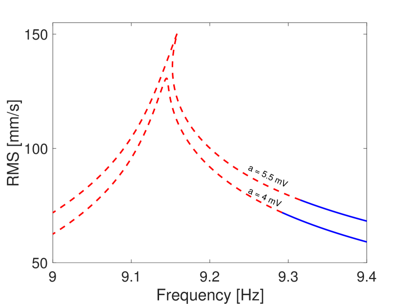
(b)

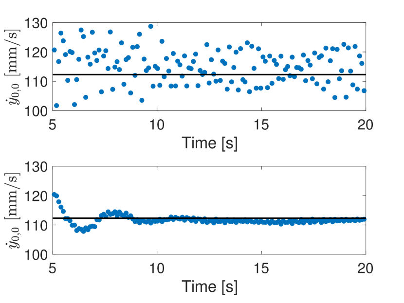
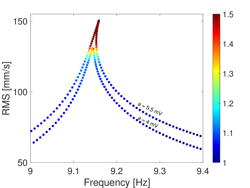
(c)

Figure 7: Frequency continuation of NLMs. (a) Continuation with respect to frequency for fixed excitation angle $\phi=\pi/2$ for the two amplitudes, $a=4$ mV and $a=5.5$ mV, that we considered in Fig. 6. (b) In the top panel, we plot the local maxima of the time series of $\dot{y}_{0,0}$ when we perturb the NLM with $f=9.3$ Hz and $a=5.5$ mV along the eigenvector that is associated with the largest-magnitude Floquet multiplier. The size of this perturbation is equal to 5% of the amplitude of the solution. We show the corresponding value of the local maximum of the NLM that we obtain via a Newton–Krylov method as the solid black line. In the bottom panel, we plot local maxima of the time series when evolving zero initial data with a fixed frequency $f=9.3$ Hz and amplitude drive $a=5.5$. (c) The same as panel (a), but with color intensity corresponding to the magnitude of the largest Floquet multiplier. Except near the peaks of the resonant curves, the instabilities are fairly weak.

In Figs. 4(d) and 6(a,b), we demonstrate that our model (3) agrees reasonably well with our experimental data. We now conduct a series of numerical computations, with parameter continuation (see Sec. III.3 for a description of our procedure), to get a better sense of the role of nonlinearity in Eq. (3) and its interplay with the disorder (at the central magnet) and the discreteness of the model. We return to our experiments in Sec. IV.4 to see what nonlinear effects we are able to capture in the laboratory.

We first perform continuation with respect to the excitation frequency $f$ for a fixed excitation angle $\phi=\pi/2$ for various values of the excitation amplitude $a$. We thereby generate nonlinear analogs of the linear resonant peak that we showed in Fig. 4(c). In Fig. 7(a), we show frequency continuations for our two drive amplitudes, $a=4$ mV and $a=5.5$, of the NLMs from Fig. 5 and Figs. 6(a,b). From comparing these frequency continuations to the linear case in Fig. 4(c), we see that the nonlinearity deforms the peak, which becomes narrower and starts to bend towards higher frequencies. The nonlinearity also destabilizes the solutions at some critical frequency; this occurs at $f\approx 9.29$ Hz for $a=4$ mV and at $f\approx 9.31$ Hz for $a=5.5$ mV. We therefore see that the NLM in Fig. 6(c) is unstable. Although our numerical computations predicted this NLM to be unstable, it is notable that we are able to access it in our experiments. Although this seems to imply that our theory is inconsistent with our experiments for the parameter values $f\approx 9.31$ Hz and $a=5.5$ mV, the instability of the NLM for these parameter values is rather weak (with $\mathrm{max}_{i}(|\sigma_{i}|)\approx 1.007$). We observe instability after many periods when we perturb the NLM along the eigenvector that is associated to the unstable Floquet multiplier $\sigma\approx 1.007$. See the top panel of Figure 7(b). However, if we initialize the dynamics with zero initial data, we approach and stay close to the NLM solution that we obtained via a Newton–Krylov method even after 200 periods of motion. See the bottom panel of Figure 7(b). This suggests that solutions with weak instabilities can still attract nearby points in phase space, at least initially, and that our numerical prediction for $f\approx 9.31$ Hz and $a=5.5$ mV is consistent with our experimental observations. Figure 7(c) is the same as Figure 7(a), but now the color scale corresponds to the magnitude of the maximum Floquet multiplier. This illustrates that the magnitude of the instability is weak throughout most of the solution branch. The instability is at its largest growth rate (with $\mathrm{max}_{i}(|\sigma_{i}|)\approx 2.15$) at the peak of the resonant curve.

(a)

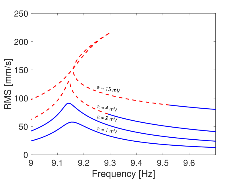
(b)

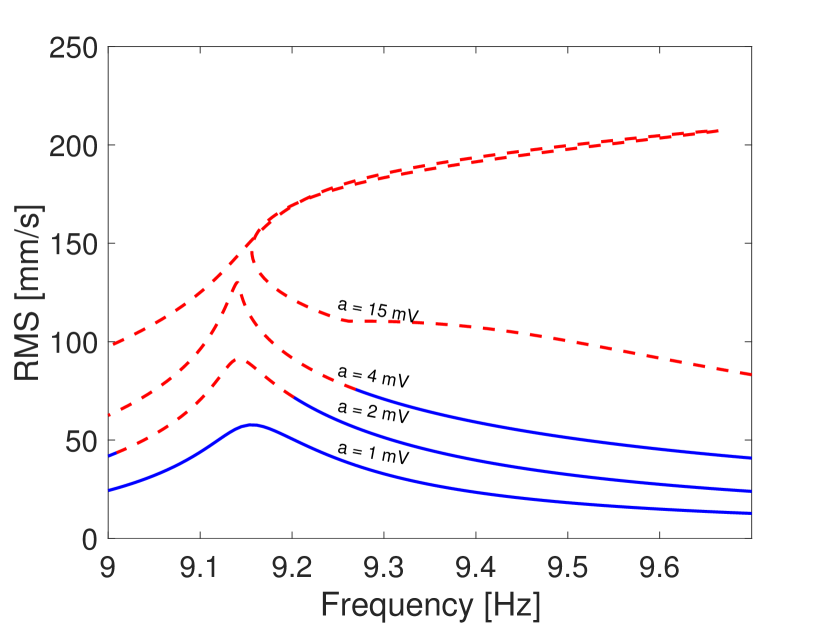
(c)

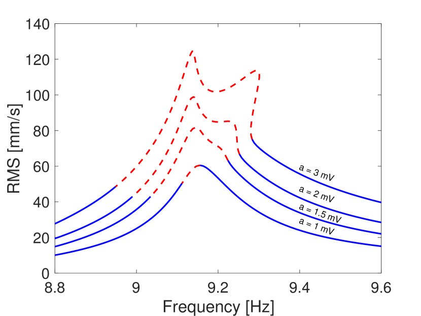
Figure 8: (a) Frequency continuation with excitation angle $\phi=\pi/2$ for excitation amplitudes $a=1$ mV, $a=2$ mV, $a=4$ mV, and $a=15$ mV (b) Frequency continuation with $\phi=0$ for $a=1$ mV, $a=2$ mV, $a=4$ mV, and $a=15$ mV (c) Frequency continuation with $\phi=\pi/3$ for $a=1$ mV, $a=1.5$ mV, $a=2$ mV, and $a=3$ mV.

In Fig. 8(a), we show the gradual bending of the resonant peak for progressively larger excitation amplitudes with $\phi=\pi/2$. In particular, for $a=15$ mV, the peak bends so far that additional solutions at $f\approx 9.3$ Hz emerge. However, these large amplitude solutions are very unstable, and we were not able to access them either in our direct numerical simulations or in our experiments. Indeed, as we will discuss in Sec. IV.4, we observe different types of dynamics at such excitation amplitudes. We can also tune the excitation angle $\phi$ and thereby deform the resonant peak in a different way. For example, when we fix the excitation angle to $\phi=0$ (i.e., an excitation along $n=0$), the resonant curves are qualitatively similar to those for $\phi=\pi/2$ for excitation amplitudes $a=1$, $a=2$, and $a=4$ [see Fig. 8(b)], although the stability properties are slightly different. For the large excitation of $a=15$ mV, the resonant curve bends even further toward higher frequencies. Even greater qualitative differences occur for $\phi=\pi/3$ (i.e., an excitation along $m=0$); see Fig. 8(c). In this case, for small-amplitude excitations, the resonant peak has a unimodal shape, as expected. However, as we consider gradually larger excitation amplitudes, an additional peak begins to emerge from the main solution branch, leading to a two-humped profile in the dependence of the RMS velocity on the frequency. This deformation is noticeable for relatively small excitation amplitudes. Specifically, we observe the existence of multiple solutions even for excitation amplitudes that are as small as $a=3$ mV, where there is bifurcation at frequency $f\approx 9.28$ Hz.

(a)

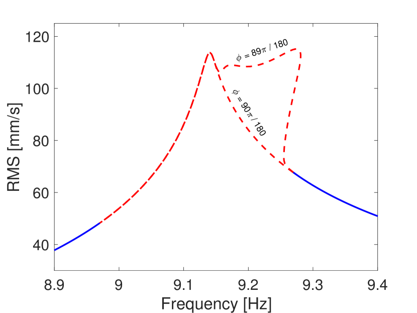
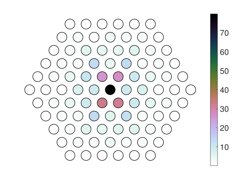
(b)

(c)

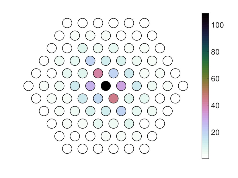
Figure 9: (a) Frequency continuation with an excitation amplitude of $a=3$ mV for two excitation angles, $\phi=89\pi/180$ and $\phi=\pi/2$. Our continuations for $\phi=89\pi/180$ and $\phi=\pi/2$ are indistinguishable when we are outside the parameter region in which the $\phi=89\pi/180$ continuation has an additional branch of NLM solutions. (b) Profile of the NLM for $f=9.2$ Hz that belongs to the lower branch (i.e., the smaller-amplitude NLM branch) of the $\phi=89\pi/180$ continuation. (b) Profile of the NLM for $f=9.2$ Hz that belongs to the upper branch of the $\phi=89\pi/180$ continuation.

The bifurcation diagram that we obtain when we use the excitation angle $\phi=\pi/3$ is more representative of “typical” angles than the special cases $\phi=\pi/2$ and $\phi=0$. For example, even by decreasing the angle slightly from $\phi=\pi/2$ to $\phi=89\pi/180$, we observe the additional branch in the frequency continuation [see Fig. 9(a)]. We show a plot of an NLM at frequency $f=9.2$ Hz that belongs to the main branch (i.e., the branch with smaller-amplitude NLMs) of the $\phi=89\pi/180$ continuation in Fig. 9(b). It has a similar profile to the NLM in Fig. 5. We show a plot of an NLM from the additional (i.e., larger-amplitude) branch at the same frequency $f=9.2$ Hz in Fig. 9(c). The solutions along this branch have secondary amplitudes in the $-\pi/3$ direction.

IV.4 Drive-Amplitude Sweeps

(a)

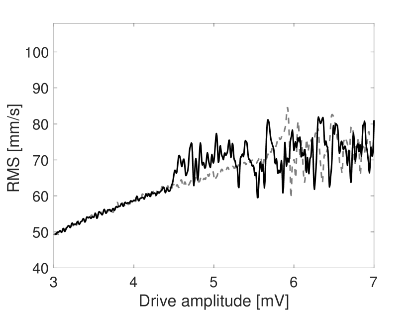
(b)

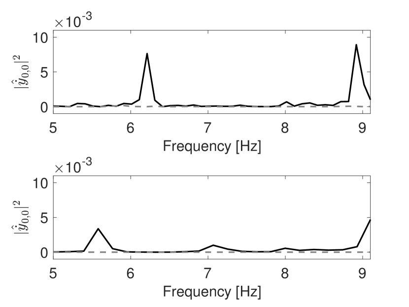
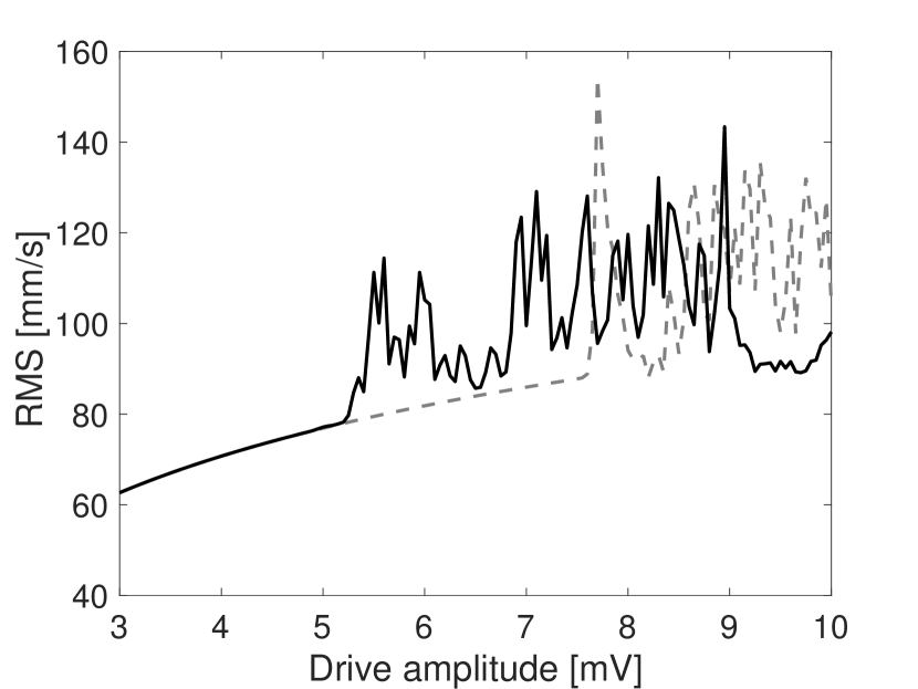
(c)

Figure 10: (a) Our upsweep (dashed gray curve) and downsweep (solid black curve) of the drive amplitude $a$ in our experiment. (b) The magnitude of the Fourier transform of the time series for the velocity of the center particle normalized by the height of the peak at $f\approx 9.3$ Hz for (top panel) our experiment and (bottom panel) numerical computation for an excitation amplitude $a=5.5$ mV. The dashed gray curve is the small-amplitude state (in the form of an NLM) that we obtain from the upsweep, and the solid black curve is the large-amplitude state that we obtain from the downsweep. (c) The upsweep (dashed gray curve) and downsweep (solid black curve) of the amplitude in our numerical simulations.

We now return to the effect of large-amplitude excitations for the parameter set — namely, $\phi=\pi/2$ and $f\approx 9.3$ Hz — in our laboratory experiments. Our bifurcation analysis revealed that the NLM solution at this parameter set destabilizes for larger amplitudes, although sometimes the instability is so weak that the NLMs are effectively stable on short enough time scales [see Fig. 7(b)]. We also observed that a large-amplitude branch of NLM solutions emerges at the parameter values $\phi=\pi/2$ and $f\approx 9.3$ Hz for sufficiently large excitation amplitudes [see Fig. 8(a)].

To study the dynamics at larger amplitudes in experiments, we initialize the system with a small-amplitude excitation (of $a=1$ mV) and gradually increase the amplitude in increments of $0.05$ mV. For each step, we run the system for 90 periods, which allows sufficient time to settle to a steady state if there is one. We record the RMS of the velocity of the center magnet for the final 5 seconds. We call this procedure an amplitude “upsweep”. We use an analogous procedure when we start with a large excitation amplitude, which we gradually decrease using the same increments. We call this procedure an amplitude “downsweep”. We show our experimental results for the upsweep and downsweep in Fig. 10(a). For sufficiently small amplitudes (specifically, for $a\lessapprox 4.5$ mV) both the upsweep and downsweep approach the same NLM, suggesting that there is a single stable branch of NLMs for $a\lessapprox 4.5$ mV. However, for $a\gtrapprox 4.5$ mV, there appear to be two different states; we obtain the small-amplitude states when we perform an upsweep and the large-amplitude states when we perform a downsweep. The small-amplitude states have the form of an NLM. The experimental result in Fig. 6(b) is an example of the small-amplitude state for $a=5.5$ mV. The large-amplitude states are also localized, but they are no longer periodic in time. An inspection of the Fourier transform of the large-amplitude state for $a=5.5$ mV reveals other peaks in the spectrum (in addition to a peak at the excitation frequency $f\approx 9.3$ Hz). In the top panel of Fig. 10(b), we show the Fourier transform of both the large-amplitude state and the small-amplitude state. The small-amplitude state (i.e., the NLM) has no peaks for lower frequencies, whereas the large-amplitude state has peaks at approximately $f=8.9$ Hz and $f=6.2$ Hz; this is suggestive of quasiperiodic behavior.

We obtain qualitatively similar results when we perform analogous upsweeps and downsweeps in numerical computations. We also observe the emergence of two states in these computations [see Fig. 10(c)]. In our computations, the large-amplitude state departs from the branch of NLMs for excitation amplitudes that are slightly larger (specifically, for $a\gtrapprox 5.1$ mV) than in our experiments. The amplitude $a\approx 5.1$ mV is roughly where the numerical NLM branch destabilizes. As in our experiments, these large-amplitude states are not periodic in time. One can also observe the presence of secondary peaks in their Fourier transforms in our numerical solutions, although the locations of these peaks are slightly different than in our experiments. See the bottom panel of Fig. 10(b). Although these numerical large-amplitude states have features that are similar to those of time-quasiperiodic states (given the multiple incommensurate peaks in the Fourier transform), it is also possible that these large-amplitude states are weakly chaotic. One issue is that we were unable to detect asymptotically stable time-quasiperiodic orbits for parameter values that correspond to the experiments. If such solutions were dynamic attractors, it would be straightforward to classify the large-amplitude states as time-quasiperiodic ones by plotting Poincaré sections of the orbits.

To clarify the nature of the large-amplitude states, we modify the parameter values slightly to obtain stable time-quasiperiodic solutions. We perform amplitude upsweeps and downsweeps for the parameter set $\phi=\pi/2$, $f=9.65$ Hz, and $M_{b}=125$ g. We use a different drive frequency from our prior calculations, because the smaller mass $M_{b}=125$ g leads to a cutoff frequency of $f_{c}\approx 9.01$ Hz and a defect frequency of $f_{d}\approx 9.36$ Hz. The amplitude sweeps with these parameter values lead to a well-defined large-amplitude branch of solutions that bifurcates from the main branch of periodic ones (the NLMs) [see Fig. 11(a)]. In Fig. 11(a), we show three solid markers to point out the locations of three solutions: a large-amplitude state that appears to be either time-quasiperiodic or time-chaotic in black, the NLM (in gray), and a stable time-quasiperiodic orbit (in red). We show a plot of a projection of the Poincaré section in the $(y,\dot{y})$ plane in Fig. 11(b) for the two states that are not time-periodic. The orbit in the bottom panel reveals a well-defined invariant curve, illustrating the quasiperiodic nature of the solution. We show the Fourier transforms of these two non-periodic states in Fig. 11(c). Both have a secondary peak in the spectrum, demonstrating that the solutions are indeed non-periodic in time (because of the incommensurate peaks in the frequency spectra). Laboratory experiments for this modified parameter set yield similar results. In particular, there is a well-defined large-amplitude branch of solutions that bifurcate from a branch of time-periodic solutions [see Fig. 11(d,e)]. The Fourier transform of one of the large-amplitude states also has a secondary peak in the spectrum, an indication that the state is nearly quasiperiodic. For simplicity, we henceforth call them simply “quasiperiodic”.

Because the numerical computations and experiments with the modified mass $M_{b}=125$ g reveal the existence of time-quasiperiodic orbits that bifurcate from the main branch of time-periodic NLMs, it is reasonable to conclude that these quasiperiodic solutions persist when we continue the parameters to the original parameter set $M_{b}=138.2$ g and $f_{d}=9.3$. This suggests that the large-amplitude branch in Fig. 10(a,c) consists of time-quasiperiodic solutions.

(a)

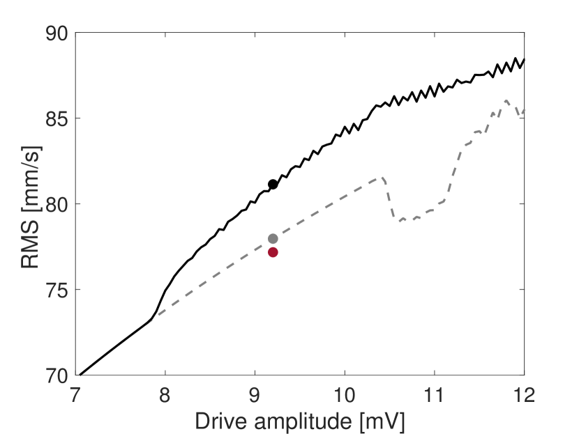
(b)

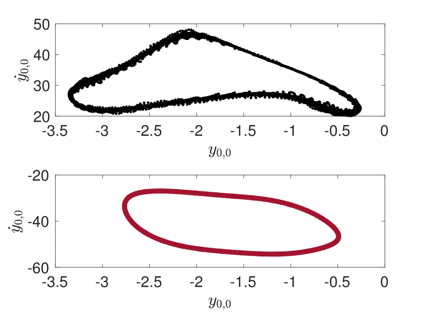
(c)

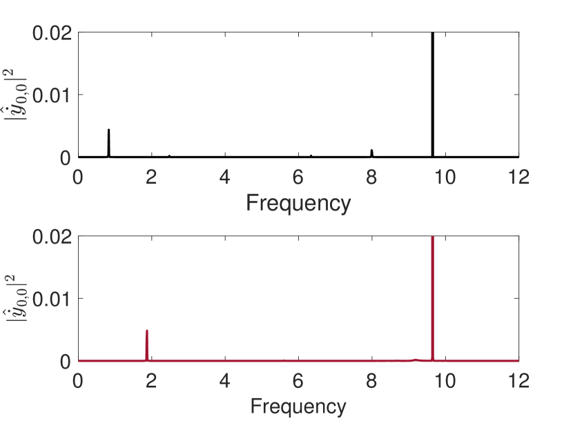
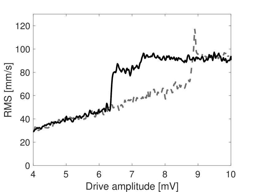
(d)

(e)

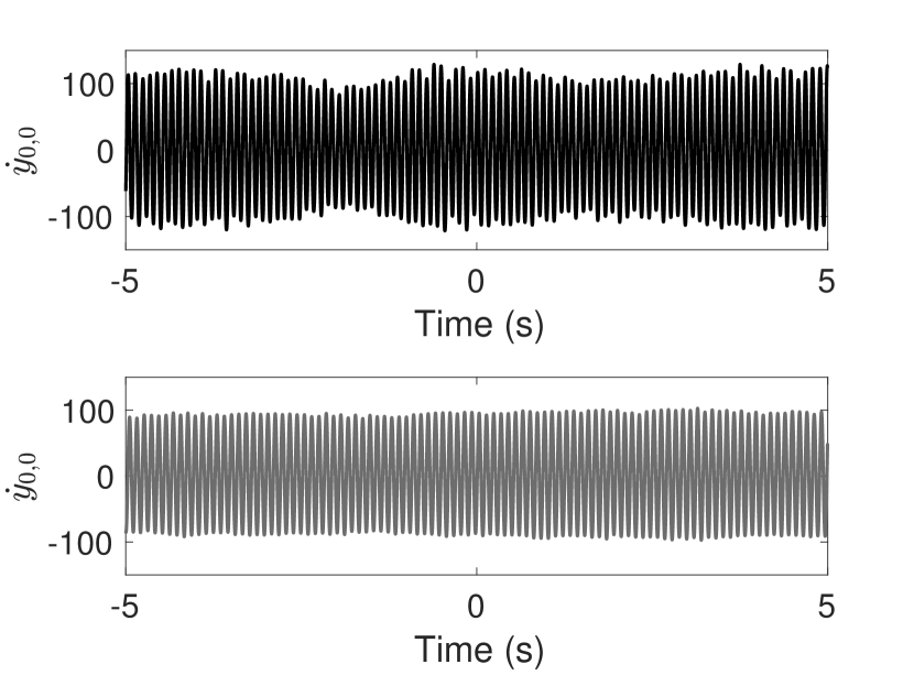
(f)

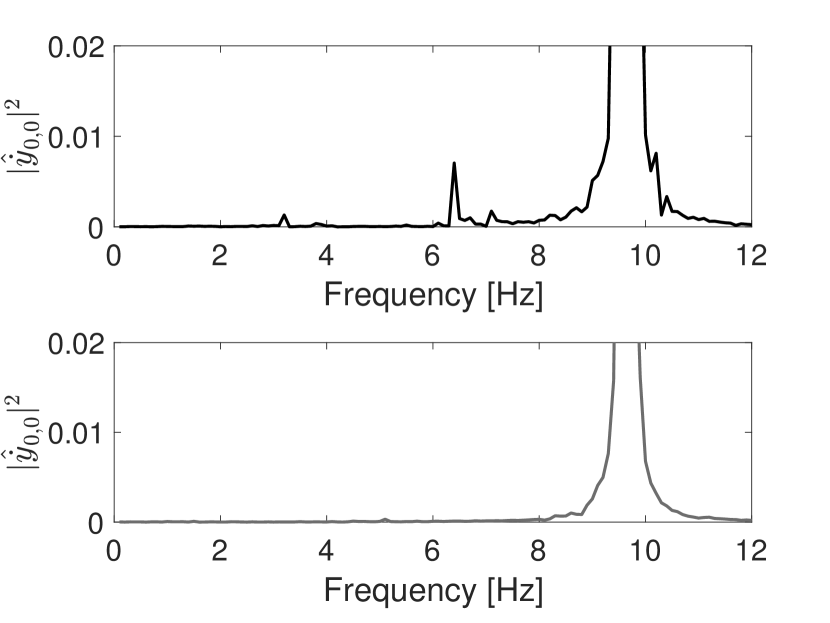
Figure 11: (a) The upsweep (dashed gray curve) and downsweep (solid black curve) for our numerical simulations with $M_{b}=125$ g and $f=9.65$ Hz. Three states exist when we use an excitation amplitude of $a=9.2$ mV. Two of the states (the black and red dots) are not periodic in time, and the other (the gray dot) is time-periodic. We obtain the state that is indicated by the red dot by simulating zero initial data for 90 periods of motion. (b) In the top panel, we show a projection of the Poincaré section of the solution that is represented by the black dot in panel (a). In the bottom panel, we show a projection of the Poincaré section of the solution that is represented by the red dot in panel (a). (c) The magnitude of the Fourier transforms of the solutions in panel (b). (d) The upsweep (dashed gray curve) and downsweep (solid black curve) for our experiments. (e) The gray curve is the experimental time series of the small-amplitude state that we obtain from the upsweep for an excitation amplitude of $a=8$ mV. The solid black curve is the time series of the large-amplitude state that we obtain from the downsweep for an excitation amplitude of $a=8$ mV. (f) The magnitude of the Fourier transform of the time series of panel (e) normalized by the height of the peak at $f=9.5$. The gray curve corresponds to the small-amplitude state, and the solid black curve corresponds to the large-amplitude state.

V Conclusions

We have demonstrated, both experimentally and numerically, the existence of nonlinear localized modes in a 2D hexagonal lattice of repelling magnets. By exploring the effects of nonlinearity numerically using frequency continuation and experimentally using amplitude sweeps, we revealed the emergence of both time-periodic NLMs and time-quasiperiodic localized states. We have also established that our experimental setup is a viable approach for fundamental studies in nonlinear lattice systems that go beyond what can occur in 1D chains. We found that the smaller-amplitude NLMs that we considered are stable, whereas progressively larger excitation amplitudes led to instabilities and more complicated dynamics, including time-quasiperiodic and potentially time-chaotic behavior. We also explored the anisotropy of the hexagonal lattice by considering different excitation angles and examining the nature and decay of the states along these angles.

Our work paves the way for many future studies. For example, although our parameter continuation in frequency revealed several families of solutions, there are undoubtedly — given the complexity of the studied system — several other ones (including possibly exotic ones) to discover. Other avenues for future work include the study of refined models — such as ones that account for nonlinear damping (or, more generally, a more elaborate form of damping rosas2007 ; vergara ; khatriprl ), rotational effects (which are often considered to be important merkel ; yuli ), and/or long-range interactions magBreathers — of our lattice system. Each of these aspects will add elements of complexity, but they also may lead to other types of interesting dynamics, such as the possibility of breather solutions with algebraically decaying tails of waves in space. It is also certainly possible that the inclusion of rotational effects and/or more sophisticated damping models may help improve matches with laboratory experiment. Such models have an associated cost of being more complicated and hence more cumbersome to analyze and simulate. Our attempt in the present paper has been to explore the principal features of the interplay of discreteness, local disorder, and nonlinearity in a hexagonal lattice of magnets. Breathers in heterogenous hexagonal magnetic lattices (e.g., ones with a repeating pattern of two masses) may lead to the existence of intrinsic localized modes and are also worthy of future study. In that context, the study of band gaps, instabilities, and nonlinear modes and their propagation is another topic of substantial ongoing interest.

Appendix

To derive the external force that the wire exerts on a magnet, we first define our coordinate system. We choose a set of orthogonal unit vectors $\hat{r}$, $\hat{z}$, and $\hat{s}$ that are centered on the wire and oriented such that the wire is aligned with the $\hat{s}$ axis [see Fig. 12(a)]. We model the magnetic moment $\mu$ of the magnet using the Gilbert model of a magnetic dipole jackson_classical_1999 ,

$${\bf F}_{\mathrm{wire}}=\left(\mu\cdot\nabla\right){\bf B}:$$ (15)

which describes the force that acts on the dipole due to the magnetic field ${\bf B}$. In our setup, the wire carries an electric current $I$ that generates the magnetic field ${\bf B}(r,z)=B_{r}(r,z)\hat{r}+B_{z}(r,z)\hat{z}$. Evaluating ${\bf B}$ at the position $-h\hat{z}+r\hat{r}$ of the magnet yields

$${\bf B}(r,-h)=\frac{I\mu_{0}}{2\pi\sqrt{h^{2}+r^{2}}}\left(\sin\theta\,\hat{r}+\cos\theta\,\hat{z}\right)\,,$$ (16)

where $\mu_{0}$ is the magnetic permeability and $\theta$ is the angle between ${\bf B}$ and $\mu$. We are interested only in the $\hat{r}$ component of the force, because we are assuming that we can neglect the dynamics along the $\hat{z}$ axis. Therefore, inserting Eq. (16) into Eq. (15) and taking $\mu=\mathcal{M}\hat{z}$, we obtain

$${\bf F}_{\mathrm{wire}}=\mathcal{M}\,\partial_{r}B_{z}(r,z)\hat{r}=\frac{I\mu_{0}\mathcal{M}}{2\pi}\frac{h^{2}-r^{2}}{(h^{2}+r^{2})^{2}}\hat{r}\,,$$ (17)

which corresponds to Eq. (1). In our coordinates, we place the wire in an orientation in the plane that is spanned by the lattice basis vectors $e_{1}=(1,0)$ and $e_{2}=(1/2,\sqrt{3}/2)$. However, it is straightforward to write Eq. (17) in coordinates in the $\{e_{1},e_{2}\}$ basis by including a parameter $\phi$ that accounts for the excitation angle. For instance, for the central magnet, we may write

$$\mathbf{F}^{\mathrm{ext}}_{0,0}=\ \ \frac{I\mu_{0}\mathcal{M}}{2\pi}\begin{pmatrix}\cos(\phi)\frac{h^{2}-x_{0,0}^{2}}{(h^{2}+x_{0,0}^{2})^{2}}\\ \sin(\phi)\frac{h^{2}-y_{0,0}^{2}}{(h^{2}+y_{0,0}^{2})^{2}}\end{pmatrix}\,,$$ (18)

which corresponds to Eq. (4).

(a)

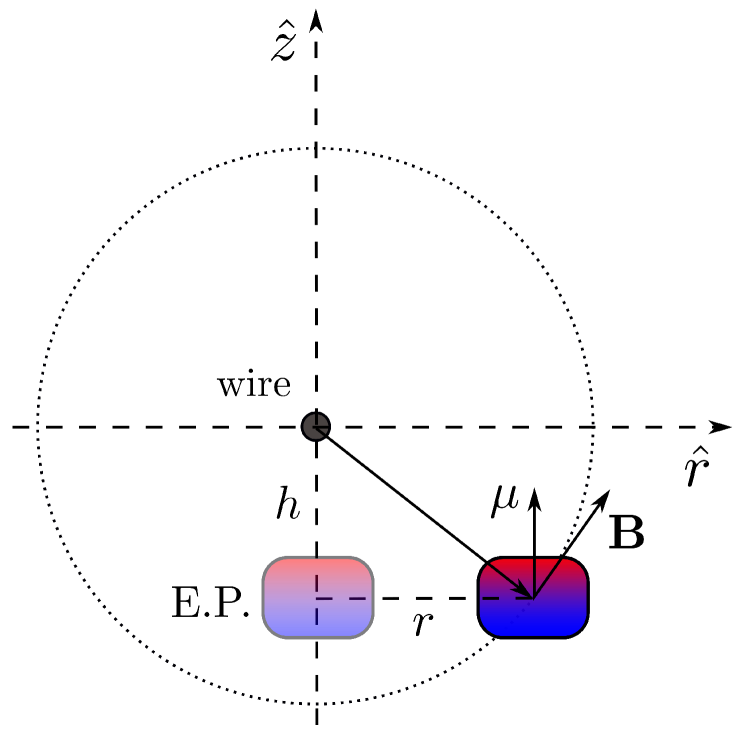
(b)

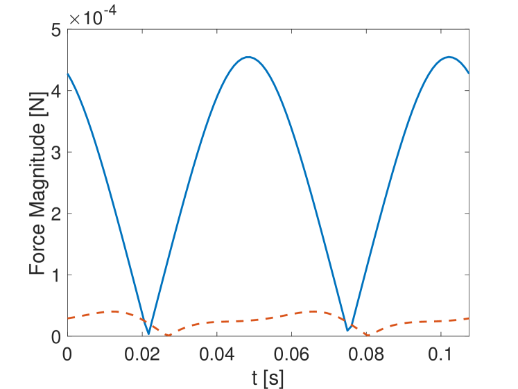
Figure 12: (a) Schematic of the interaction between a single magnet and a wire in the $(\hat{r},\hat{z})$ plane, which is orthogonal to the direction of the wire. We use “E.P.” to denote the equilibrium position of the magnet. (b) Squared magnitudes of the forces that result from lattice interactions (solid blue curve) and the external drive from the wire (dashed red curve) for the NLM from Fig. 5(a) during one period of motion. Specifically, we plot $|\mathbf{F}^{\mathrm{lattice}}_{0,0}(t)|^{2}$ using the solid blue curve and $|\mathbf{F}^{\mathrm{ext}}_{0,0}(t)|^{2}$ using the dashed red curve.

Although the form of the force that describes the external drive is specific to our experimental setup, the dynamics are dominated by the lattice forces. For example, in Fig. 12(b), we compare the forces that result from the wire (see Eq. (18)) and the force from the lattice for the NLM of Fig. 5(a). The lattice forces are

$$\begin{array}[]{ll}\displaystyle\mathbf{F}^{\mathrm{lattice}}_{m,n}=&-\mathbf{F}_{0}(\mathbf{q}_{m+1,n}-\mathbf{q}_{m,n})-\mathbf{F}_{1}(\mathbf{q}_{m,n+1}-\mathbf{q}_{m,n})+\mathbf{F}_{-1}(\mathbf{q}_{m,n}-\mathbf{q}_{m-1,n+1})\\ &+\mathbf{F}_{0}(\mathbf{q}_{m,n}-\mathbf{q}_{m-1,n})+\mathbf{F}_{1}(\mathbf{q}_{m,n}-\mathbf{q}_{m,n-1})-\mathbf{F}_{-1}(\mathbf{q}_{m+1,n-1}-\mathbf{q}_{m,n})\end{array}$$ (19)

However, it is also important to acknowledge that the effective “defect” that is produced by the force (19) is responsible for the presence of the corresponding linear defect frequency and hence for the associated NLMs in the presence of nonlinearity.

References

- (1) F. Lederer, G. I. Stegeman, D. N. Christodoulides, G. Assanto, M. Segev, and Y. Silberberg, “Discrete solitons in optics,” Phys. Rep., vol. 463, p. 1, 2008.
- (2) P. Binder, D. Abraimov, A. V. Ustinov, S. Flach, and Y. Zolotaryuk, “Observation of breathers in Josephson ladders,” Phys. Rev. Lett., vol. 84, p. 745, 2000.
- (3) E. Trías, J. J. Mazo, and T. P. Orlando, “Discrete breathers in nonlinear lattices: Experimental detection in a Josephson array,” Phys. Rev. Lett., vol. 84, p. 741, 2000.
- (4) L. Q. English, M. Sato, and A. J. Sievers, “Modulational instability of nonlinear spin waves in easy-axis antiferromagnetic chains. II. influence of sample shape on intrinsic localized modes and dynamic spin defects,” Phys. Rev. B, vol. 67, p. 024403, 2003.
- (5) U. T. Schwarz, L. Q. English, and A. J. Sievers, “Experimental generation and observation of intrinsic localized spin wave modes in an antiferromagnet,” Phys. Rev. Lett., vol. 83, p. 223, 1999.
- (6) B. I. Swanson, J. A. Brozik, S. P. Love, G. F. Strouse, A. P. Shreve, A. R. Bishop, W.-Z. Wang, and M. I. Salkola, “Observation of intrinsically localized modes in a discrete low-dimensional material,” Phys. Rev. Lett., vol. 82, p. 3288, 1999.
- (7) M. Peyrard, “Nonlinear dynamics and statistical physics of DNA,” Nonlinearity, vol. 17, p. R1, 2004.
- (8) J. Bajars, J. C. Eilbeck, and B. Leimkuhler, Numerical Simulations of Nonlinear Modes in Mica: Past, Present and Future, vol. 221, p. 35. Cham, Switzerland: Springer International Publishing, 2015.
- (9) O. Morsch and M. Oberthaler, “Dynamics of Bose–Einstein condensates in optical lattices,” Rev. Mod. Phys., vol. 78, p. 179, 2006.
- (10) S. Flach and A. Gorbach, “Discrete breathers: Advances in theory and applications,” Phys. Rep., vol. 467, p. 1, 2008.
- (11) P. G. Kevrekidis, “Non-linear waves in lattices: Past, present, future,” IMA J. Appl. Math., vol. 76, pp. 389–423, 2011.
- (12) S. V. Dmitriev, E. A. Korznikova, Y. A. Baimova, and M. G. Velarde, “Discrete breathers in crystals,” Physics-Uspekhi, vol. 59, pp. 446–461, may 2016.
- (13) E. Fermi, J. Pasta, and S. Ulam, “Studies of Nonlinear Problems. I.,” (Los Alamos National Laboratory, Los Alamos, NM, USA), vol. Tech. Rep., pp. LA–1940, 1955.
- (14) G. Gallavotti, The Fermi–Pasta–Ulam Problem: A Status Report. Heidelberg, Germany: Springer-Verlag, 2008.
- (15) V. F. Nesterenko, Dynamics of Heterogeneous Materials. Heidelberg, Germany: Springer-Verlag, 2001.
- (16) C. Chong and P. G. Kevrekidis, Coherent Structures in Granular Crystals: From Experiment and Modelling to Computation and Mathematical Analysis. Heidelberg, Germany: Springer-Verlag, 2018.
- (17) Y. Starosvetsky, K. R. Jayaprakash, M. A. Hasan, and A. F. Vakakis, Topics On The Nonlinear Dynamics And Acoustics Of Ordered Granular Media. World Scientific, Singapore, 2017.
- (18) C. Chong, M. A. Porter, P. G. Kevrekidis, and C. Daraio, “Nonlinear coherent structures in granular crystals,” J. Phys. Cond. Matt., vol. 29, p. 413003, 2017.
- (19) M. Molerón, A. Leonard, and C. Daraio, “Solitary waves in a chain of repelling magnets,” J. App. Phys., vol. 115, no. 18, p. 184901, 2014.
- (20) A. Mehrem, N. Jiménez, L. J. Salmerón-Contreras, X. García-Andrés, L. M. García-Raffi, R. Picó, and V. J. Sánchez-Morcillo, “Nonlinear dispersive waves in repulsive lattices,” Phys. Rev. E, vol. 96, p. 012208, 2017.
- (21) M. Serra-Garcia, M. Molerón, and C. Daraio, “Tunable, synchronized frequency down-conversion in magnetic lattices with defects,” Phil. Trans. Roy. Soc. A: Math. Phys. Eng. Sci., vol. 376, no. 2127, p. 20170137, 2018.
- (22) J. L. Marín, J. C. Eilbeck, and F. M. Russell, 2-D Breathers and Applications, vol. 542, p. 293. Heidelberg, Germany: Springer-Verlag, 2000.
- (23) L. Q. English, F. Palmero, J. F. Stormes, J. Cuevas, R. Carretero-González, and P. G. Kevrekidis, “Nonlinear localized modes in two-dimensional electrical lattices,” Phys. Rev. E, vol. 88, p. 022912, 2013.
- (24) S. Vladimirov and K. Ostrikov, “Dynamic self-organization phenomena in complex ionized gas systems: New paradigms and technological aspects,” Phys. Rep., vol. 393, no. 3, pp. 175–380, 2004.
- (25) V. Koukouloyannis, P. G. Kevrekidis, K. J. H. Law, I. Kourakis, and D. J. Frantzeskakis, “Existence and stability of multisite breathers in honeycomb and hexagonal lattices,” J. Phys. A: Math. Theor., vol. 43, no. 23, p. 235101, 2010.
- (26) J. A. D. Wattis, Asymptotic Approximation of Discrete Breather Modes in Two-Dimensional Lattices, vol. 221, p. 179. Heidelberg, Germany: Springer-Verlag, 2015.
- (27) S. Flach, K. Kladko, and S. Takeno, “Acoustic breathers in two-dimensional lattices,” Phys. Rev. Lett., vol. 79, pp. 4838–4841, 1997.
- (28) J. L. Marín, J. C. Eilbeck, and F. M. Russell, “Localized moving breathers in a 2D hexagonal lattice,” Phys. Lett. A, vol. 248, no. 2, pp. 225–229, 1998.
- (29) B.-B. Lü and T. Qiang, “Discrete gap breathers in a two-dimensional diatomic face-centered square lattice,” Chinese Physics B, vol. 18, no. 10, p. 4393, 2009.
- (30) V. Koukouloyannis and I. Kourakis, “Discrete breathers in hexagonal dusty plasma lattices,” Phys. Rev. E, vol. 80, p. 026402, 2009.
- (31) B.-F. Feng and T. Kawahara, “Discrete breathers in two-dimensional nonlinear lattices,” Wave Motion, vol. 45, no. 1, pp. 68 – 82, 2007.
- (32) A. A. Maradudin, E. W. Montroll, and G. H. Weiss, Theory of Lattice Dynamics in the Harmonic Approximation. New York City, NY, USA: Academic Press, 1963.
- (33) G. Theocharis, M. Kavousanakis, P. G. Kevrekidis, C. Daraio, M. A. Porter, and I. G. Kevrekidis, “Localized breathing modes in granular crystals with defects,” Phys. Rev. E, vol. 80, p. 066601, 2009.
- (34) N. Boechler, G. Theocharis, and C. Daraio, “Bifurcation based acoustic switching and rectification,” Nat. Mater., vol. 10, no. 9, p. 665, 2011.
- (35) C. Hoogeboom, Y. Man, N. Boechler, G. Theocharis, P. G. Kevrekidis, I. G. Kevrekidis, and C. Daraio, “Hysteresis loops and multi-stability: From periodic orbits to chaotic dynamics (and back) in diatomic granular crystals,” Euro. Phys. Lett., vol. 101, p. 44003, 2013.
- (36) C. Chong, A. Foehr, E. G. Charalampidis, P. G. Kevrekidis, and C. Daraio, “Breathers and other time-periodic solutions in an array of cantilevers decorated with magnets,” Math. Eng., vol. 1, pp. 489–507, 2019.
- (37) M. Molerón, C. Chong, A. J. Martínez, M. A. Porter, P. G. Kevrekidis, and C. Daraio, “Nonlinear excitations in magnetic lattices with long-range interactions,” New J. Phys., vol. 21, p. 063032, 2019.
- (38) S. Flach, “Breathers on lattices with long range interaction,” Phys. Rev. E, vol. 58, pp. R4116–R4119, 1998.
- (39) R. F. Steidel, An Introduction to Mechanical Vibrations. New York City, NY, USA: John Wiley & Sons, Inc., 1989.
- (40) C. T. Kelley, Solving Nonlinear Equations with Newton’s Method. Philadelphia, PA, USA: Society for Industrial and Applied Mathematics, 2003.
- (41) E. Doedel and L. S. Tuckerman, Numerical Methods for Bifurcation Problems and Large-Scale Dynamical Systems. Heidelberg, Germany: Springer-Verlag, 2000.
- (42) M. W. Hirsch, S. Smale, and R. L. Devaney, Differential Equations, Dynamical Systems, and an Introduction to Chaos. Amsterdam, The Netherlands: Elsevier, 2004.
- (43) B. A. Malomed, “Potential of interaction between two- and three-dimensional solitons,” Phys. Rev. E, vol. 58, pp. 7928–7933, Dec 1998.
- (44) R. J. Decker, A. Demirkaya, N. S. Manton, and P. G. Kevrekidis, “Kink–antikink interaction forces and bound states in a biharmonic model,” arXiv:2005.04523, 2020.
- (45) A. Rosas, A. H. Romero, V. F. Nesterenko, and K. Lindenberg, “Observation of two-wave structure in strongly nonlinear dissipative granular chains,” Phys. Rev. Lett., vol. 98, p. 164301, 2007.
- (46) L. Vergara, “Model for dissipative highly nonlinear waves in dry granular systems,” Phys. Rev. Lett., vol. 104, p. 118001, 2010.
- (47) R. Carretero-González, D. Khatri, M. A. Porter, P. G. Kevrekidis, and C. Daraio, “Dissipative solitary waves in granular crystals,” Phys. Rev. Lett., vol. 102, p. 024102, 2009.
- (48) A. Merkel, V. Tournat, and V. Gusev, “Experimental evidence of rotational elastic waves in granular phononic crystals,” Phys. Rev. Lett., vol. 107, p. 225502, 2011.
- (49) K. Vorotnikov, M. Kovaleva, and Y. Starosvetsky, “Emergence of non-stationary regimes in one- and two-dimensional models with internal rotators,” Phil. Trans. A: Math. Phys. Eng. Sci., vol. 376, p. 20170134, 2018.
- (50) J. D. Jackson, Classical Electrodynamics. New York City, NY, USA: John Wiley & Sons, Inc., 3rd ed. ed., 1999.