ALICE: Active Learning with Contrastive Natural Language Explanations

Abstract

Training a supervised neural network classifier typically requires many annotated training samples. Collecting and annotating a large number of data points are costly and sometimes even infeasible. Traditional annotation process uses a low-bandwidth human-machine communication interface: classification labels, each of which only provides a few bits of information. We propose Active Learning with Contrastive Explanations (ALICE), an expert-in-the-loop training framework that utilizes contrastive natural language explanations to improve data efficiency in learning. ALICE learns to first use active learning to select the most informative pairs of label classes to elicit contrastive natural language explanations from experts. Then it extracts knowledge from these explanations using a semantic parser. Finally, it incorporates the extracted knowledge through dynamically changing the learning model’s structure. We applied ALICE in two visual recognition tasks, bird species classification and social relationship classification. We found by incorporating contrastive explanations, our models outperform baseline models that are trained with 40-100% more training data. We found that adding $1$ explanation leads to similar performance gain as adding 13-30 labeled training data points.

1 Introduction

The de-facto supervised neural network training paradigm requires a large dataset with annotations. It is time-consuming, difficult and sometimes even infeasible to collect a large number of data-points due to task nature. A typical example task is medical diagnosis. In addition, annotating datasets also is costly, especially in domains where experts are difficult to recruit. In a traditional annotation process, the human-machine communication bandwidth is narrow. Each label provides $\log C$ bits per sample for a $C$-class classification problem. However, humans don’t solely rely on such low bandwidth communication to learn. They instead learn through natural language communication, which grounds on abstract concepts and knowledge. Psychologists and philosophers have long posited natural language explanations as central, organizing elements to human learning and reasoning Chin-Parker and Cantelon (2017); Lombrozo (2006); Smith (2003). Following this intuition, we explore methods to incorporate natural language explanations in learning paradigms to improve learning algorithm’s data efficiency.

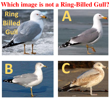
Figure 1: An example task that would benefit from learning with natural language explanation. The top-left corner shows an example image of a ring-billed gull. In the other three images (A), (B), (C), which one is not a ring-billed gull but a California gull? Given the natural language explanation “Ring-billed gull has a bill with a black ring near the tip while California gull has a red spot near the tip of lower mandible”, it would be easier to find that (A) is the correct choice.

Let’s take a bird species classification task as an example to illustrate the advantage of learning with natural language explanation. Figure 1 shows several bird images. Based on visual dissimilarity, many people mistakenly thought Image C is not a ring-billed gull as it has a different colored coat compared to the example. However, ring-billed gulls change their coat color from light yellow to grey after the first winter. So color is not the deciding factor to distinguish California gull and ring-billed gull. If we receive abstract knowledge from human experts through a natural language format, such as “Ring-billed gull has a bill with a black ring near the tip while California gull has a red spot near the tip of lower mandible” and incorporate it in the model, then the model will discover that Image A is a California gull instead of a ring-billed gull based on its bill.

Previous work has shown that incorporating natural language explanation into the classification training loop is effective in various settings Andreas et al. (2018); Mu et al. (2020). However, previous work neglects the fact that there is usually a limited time budget to interact with domain experts (e.g., medical experts, biologists) Liang et al. (2019, 2020) and high-quality natural language explanations are expensive, by nature. Therefore, we focus on eliciting fewer but more informative explanations to reduce expert involvement.

We propose Active Learning with Contrastive Explanations (ALICE), an expert-in-the-loop training framework that utilizes contrastive natural language explanations to improve data efficiency in learning. Although we focus on image classification in this paper, our expert-in-the-loop training framework could be generalized to other classification tasks. ALICE learns to first use active learning to select the most informative query pair to elicit contrastive natural language explanations from experts. Then it extracts knowledge from these explanations using a semantic parser. Finally, it incorporates the extracted knowledge through dynamically updating the learning model’s structure. Our experiments on bird species classification and social relationship classification show that our method that incorporates natural language explanations has better data efficiency compared to methods that increase training sample volume.

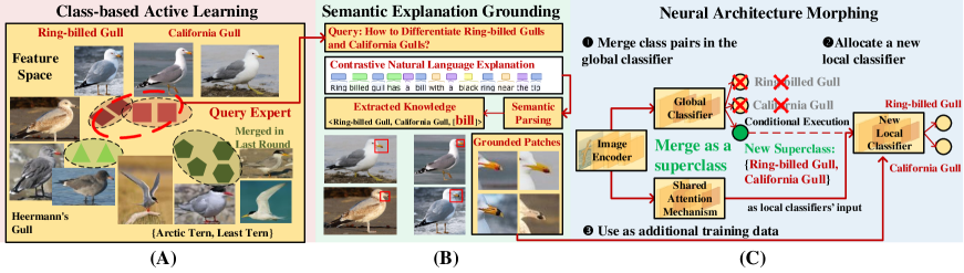
Figure 2: ALICE’s three-step workflow for each round. (A) Class-based Active Learning: ALICE first projects each class’s training data into a shared feature space. Then ALICE selects $b$ most confusing class pairs to query domain experts for explanations. (B) Semantic Explanation Grounding: ALICE then extracts knowledge from $b$ contrastive natural language explanations by semantic parsing. ALICE grounds the extracted knowledge on the training data of $b$ class pairs by cropping the corresponding semantic segments. (C) Neural Architecture Morphing: ALICE finally allocates $b$ new local classifiers and merges $b$ class pairs in the global classifier. The cropped image patches are used as additional training data for a newly added local classifier to emphasize these patches’ importance. The model is re-trained after each round.

2 Related Work

Learning with Natural Language Explanation

Psychologists and philosophers have long posited natural language explanations as central organizing elements to human learning and reasoning Chin-Parker and Cantelon (2017). Several attempts have been made to incorporate natural language explanations into supervised classification tasks. Andreas et al. (2018); Mu et al. (2020) adopt a multi-task setting by learning classification and captioning simultaneously. Murty et al. (2020); He and Peng (2017) encode natural language explanations as additional features to assist classification. Orthogonal to their approaches, we focus on eliciting fewer but more informative explanations to reduce expert involvement with class-based active learning. Another line of research collects heuristic rules as explanations (e.g., ‘honey month’ for predicting SPOUSE relationship) to automatically label unlabeled data Srivastava et al. (2017); Zhou et al. (2020); Hancock et al. (2018). Different from their settings, we assume no additional training data-points. In addition, we leverage natural language explanations by extracting knowledge and incorporate the knowledge into classifiers. Distantly related to our work, Hendricks et al. (2016) propose to generate explanations for image classifiers but they do not explore improving the classifiers with the explanations.

Active Learning

The key hypothesis of active learning is that, if the learning algorithm is allowed to choose the data from which it learns, it will perform better than randomly selecting training samples  Settles (2009). Existing work in active learning focuses primarily on exploring sampling methods to select additional data-points to label from a pool of unlabeled data Sener and Savarese (2018); Settles (2011, 2009).  Luo and Hauskrecht (2017) propose group-based active learning where the annotator could label a group of data points each time rather than one data point. However, they still rely on classification labels as the interface for human-machine communication. Instead, we focus on incorporating natural language explanations into the classification training framework. Contrastive learning has previously been shown to substantially improve unsupervised learning Abid et al. (2018), feature learning Zou et al. (2015), and learning probabilistic models Zou et al. (2013). However, it has not been applied to the setting of active learning with explanations as we explore here.

Hierarchical Visual Recognition

Categorical hierarchy is inherent in visual recognition Biederman (1987); Feng et al. (2019). Xiao et al. (2014) propose to expand the model based on category hierarchy for incremental learning. Yan et al. (2015) decompose classification task into a coarse category classification and a fine category classification. Different from previous work, we focus on incorporating contrastive natural language explanations into the model hierarchy to achieve better data efficiency.

3 Problem Formulation

Contrastive Natural Language Explanations

Existing research in social science and cognitive science Miller (2019); Mittelstadt et al. (2019) suggests contrastive explanations are more effective in human learning than descriptive explanations. Therefore, we choose contrastive natural language explanations to benefit our learners. An example contrastive explanation is like “Why P rather than Q?”, in which P is the target event and Q is a counterfactual contrast case that did not occur Lipton (1990). In the example in Figure 1, if we ask the expert to differentiate between Ring-billed gull against California gull, the expert would output the following natural language explanation: “Ring-billed gull has a bill with a black ring near the tip while California gull has a red spot near tip of lower mandible”. Our explanations are class-based and are not specifically associated with any particular images.

Problem Setup

We are interested in a $C$ class classification problem defined over an input space $X$ and a label space $Y=\{1,...,C\}$. Initially, the training set $D_{train}=\{(x_{i},y_{i})\}^{N_{train}}_{1}$ is small, since our setting is restricted to be low resource. We also assume that there is a limited budget to ask domain experts to provide explanations during training. Specifically, we consider $k$ rounds of interactions with domain experts and each round has a query budget $b$. For each query, we need to specify two classes $y^{p},y^{q}$ for domain experts to compare. Domain experts would return a contrastive natural language explanation $e$. Each explanation $e$ would guide us to focus on the most discriminating semantic segments to differentiate between $y^{p}$ and $y^{q}$. In this paper, a semantic segment refers to a semantic segment of an object (e.g., “bill” in bird species classification) or a semantic object (e.g., “soccer” in social relationship classification).

To make our framework more general, we start from a standard image classification neural architecture. We formulate our initial model as $M(\phi,g_{pool},f)=f(g_{pool}(\phi(x)))$: Here $\phi$ is an image encoder that maps each input image $x$ to an activation map $\phi(x)\in\mathbb{R}^{H\times W\times d}$. $g_{pool}$ is a global pooling layer $g_{pool}(\phi(x))\in\mathbb{R}^{d_{pool}}$. $f$ is a fully connected layer that performs flat $C$ way classification. This formulation covers most of the off-the-shelf pre-trained image classifiers.

4 ALICE: Active Learning with Contrastive Explanations

4.1 Overview

ALICE is an expert-in-the-loop training framework that utilizes contrastive natural language explanations to improve data efficiency in learning. ALICE performs multiple rounds of interaction with domain experts and dynamically updates the learning model’s structure during each round. Figure 2 describes ALICE’s three-step workflow for each round: (A) Class-based Active Learning: ALICE first projects each class’s training data into a shared feature space. Then ALICE selects $b$ most confusing class pairs to query domain experts for explanations. (B) Semantic Explanation Grounding: ALICE then extracts knowledge from $b$ contrastive natural language explanations by semantic parsing. ALICE grounds the extracted knowledge on the training data of $b$ class pairs by cropping the corresponding semantic segments. (C) Neural Architecture Morphing: ALICE finally allocates $b$ new local classifiers and merges $b$ class pairs in the global classifier. The cropped image patches are used as additional training data for a newly added local classifier to emphasize these patches’ importance. The model is re-trained after each round.

4.2 Class-based Active Learning

ALICE optimizes towards requesting the most informative explanations to reduce expert involvement. Since each explanation provides knowledge to distinguish a class pair, we aim to identify the class pairs that confuse the model most and the explanations on these class pairs would intuitively help the model a lot. ALICE identifies confusing class pairs by first projecting each class’s training data into a shared feature space $g_{pool}(\phi(x))$. As shown in Figure 2 (A), if the training data of two classes are close in the feature space, it is usually hard for the model to distinguish them and thus it would be helpful to solicit an explanation on this class pair. Based on this intuition, we first define the distance between two classes and then select the class pairs with the lowest distance. We first profile each class $j$ by fitting a multivariate Gaussian distribution $\mathcal{N}_{j}(\mu_{j},\,\Sigma_{j})$ on class $j$’s training sample features. We define the distance between class $j$ and class $k$ as the Jensen–Shannon Divergence (JSD) between $\mathcal{N}_{j}$ and $\mathcal{N}_{k}$.

$$\mathbb{D}_{\mathsf{J}}(\mathcal{N}_{j},\mathcal{N}_{k})\triangleq\frac{1}{2}\mathbb{D}_{\mathsf{KL}}(\mathcal{N}_{j}||(\mathcal{N}_{jk}))+\frac{1}{2}\mathbb{D}_{\mathsf{KL}}(\mathcal{N}_{k}||\mathcal{N}_{jk})$$

where $\mathcal{N}_{jk}=\frac{1}{2}(\mathcal{N}_{j}+\mathcal{N}_{k})$ and $\mathbb{D}_{\mathsf{KL}}(\mathcal{N}_{j}||\mathcal{N}_{k})$ is the Kullback-Liebler (KL) divergence:

$$\mathbb{D}_{\mathsf{KL}}(\mathcal{N}_{j}||\mathcal{N}_{k})= \frac{1}{2}\Big{(}tr(\Sigma_{k}^{-1}\Sigma_{j}-I)+\log(\frac{|\Sigma_{k}|}{|\Sigma_{j}|})$$

$$+(\mu_{j}-\mu_{k})^{T}\Sigma_{k}^{-1}(\mu_{j}-\mu_{k})\Big{)}$$

After calculating the distance between all possible class pairs, we select the $b$ class pairs with the lowest JSD distance to query domain experts.

4.3 Semantic Explanation Grounding

After identifying $b$ class pairs that the model is most confused about, we send $b$ query to domain experts. We ask the expert the following question for each query, “How would you differentiate class $P$ and class $Q$?”. Since we want the expert to provide general class-level knowledge, each query only contains text information, and no visual examples are provided to the experts. We obtain $b$ contrastive natural language explanations after the query. Next, we parse the natural language explanations into machine-understandable form.

Query Expert: “How to differentiate Ring-billed Gulls and California Gulls?”
Parse Expert Explanation: “Ring-billed Gull has a bill with a black ring near the tip while California Gull has a red spot near the tip of lower mandible. ”
Extracted Knowledge: Pay attention to [Bill] when classifying Ring-billed Gull v.s. California Gulls
Ground Extracted Knowlwdge: Crop [Bill] in every training image of Ring-billed Gulls and California Gulls

Table 1: Semantic Explanation Grounding Workflow

We choose a simple rule-based semantic parser for simplicity, following Hancock et al. (2018). The simple rule-based semantic parser can be used without any additional training and requires minimum effort to develop. Formally, the parser uses a set of rules in the form $\alpha\rightarrow\beta$, which means that $\alpha$ can be replaced by the token(s) in $\beta$. Our rules focus primarily on identifying the discriminating semantic segments ($\S$ 3) mentioned in the explanations (e.g., “bill” for differentiating between ring-billed gull and California gull). We also allow the parser to skip unexpected tokens so that the parser could always succeed in generating a valid output.

Since each explanation $e$ provides class-level knowledge to distinguish class $y^{p},y^{q}$, we need to propagate the knowledge to all the training data-points in class $y^{p},y^{q}$ so that the learning model could incorporate the knowledge later during training. We denote the semantic segments mentioned in an explanation $e$ as $S=\{s_{1},s_{2},...,\}$. For each training data-point of class $y^{p},y^{q}$, we apply off-the-shelf semantic segment localization models to crop out the image patch(es) of the semantic segment(s) mentioned $S=\{s_{1},s_{2},...,\}$ (Figure 2 (B)). The number of patches cropped from each image equals the number of mentioned semantic segments (i.e., $|S|$). We then resize the image patches to full resolution. The intuition behind our crop-and-resize approach comes from the popular image crop data augmentation: it augments the training data with “sampling of various sized patches of the image whose size is distributed evenly between 8% and 100% of the image area” Szegedy et al. (2015). This data augmentation technique is widely-adopted and is supported by common deep learning frameworks like PyTorch.

ALICE does not need the localization model during testing (More details in $\S$ 4.4). The off-the-shelf semantic segment localization models could be the pre-trained localization models on various large-scale datasets like Visual Genome Krishna et al. (2017) and PASCAL-Part Chen et al. (2014). If there is no available off-the-shelf localization model, we could recruit non-expert annotators to annotate the location of the semantic segments given that our training set $D_{train}$ is small.

4.4 Neural Architecture Morphing

Overview

ALICE incorporates contrastive natural language explanations through dynamically updating the learning model’s structure. The high-level idea is to allocate a number of local classifiers to help the origin model guided by the explanations. Specifically, for each explanation $e$ that provides knowledge to distinguish two classes $y_{p},y_{q}$, we allocate a local classifier that is dedicated to the binary classification between $y_{p},y_{q}$. We incorporate the extracted knowledge from explanation $e$ to the local classifier so that the local classifier learns to focus on the discriminating semantic segments pointed out by the domain experts. We first discuss the case where all local classifiers perform binary classification and then discuss how to extend them to support general m-ary classification.

Progressive Architecture Update

The initial flat $C$-way classification architecture could be viewed as a composition of an image encoder $\phi$ and a global classifier $f\circ g_{pool}$. We discuss how the local classifiers are progressively added to assist the global classifier. As shown in Figure 2 (C), we first merge $b$ class pairs into $b$ super-classes in the global classifier. For example, in the first round, the global classifier would change from $C$-way to $(C-2b+b)$-way. We then allocate $b$ new local classifiers, each for performing binary classification for one class pair. Each local classifier is only called when the global classifier predicts its super-class as the most confident. We delay more complex conditional execution schemes as future work. We also note that the conditional execution schemes have potential for reducing computation runtime Chen et al. (2020); Mailthody et al. (2019). During training, we fine-tune the image encoder $\phi$ and reset the global classifier after each round since it is only a linear layer.

Knowledge Grounded Training

The global classifier is trained on $D_{train}$, with labels adjusted according to the class pair merging. For a local classifier corresponding to the class pair $y^{p},y^{q}$, its training data consists of two parts. One part of the training data is the training data-points of classes $y^{p},y^{q}$ in $D_{train}$. The other part is the resized image patches of class $y^{p},y^{q}$ obtained in semantic explanation grounding ($\S$ 4.3). We use the resized image patches as additional training data to to emphasize these patches’ importance. Take the local classifier distinguishing ring-billed gull and California gull as an example (Figure 2 (B, C)). This local classifier is trained on the training images of ring-billed gull and California gull, as well as the bills’ patches of each training image of ring-billed gull and California gull. During testing, we only feed the whole image into the model.

Supporting m-ary local classifier

So far we have assumed that the local classifier is always a binary classifier. An implicit assumption is that the $b$ class pairs have no overlap. We could support overlapping class pairs as follows. If some class pairs have overlap (e.g., class pair $(P,Q)$, class pair $(P,T)$, class pair $(T,U)$), we only allocate one local classifier for them (e.g., a $4$-ary local classifier for class $(P,Q,T,U)$). We also merge all the relevant classes in the global classifier into only one super-class (e.g., super-class $\{P,Q,T,U\}$). The local classifier is trained on the union of the overlapping class pairs’ training data including patches.

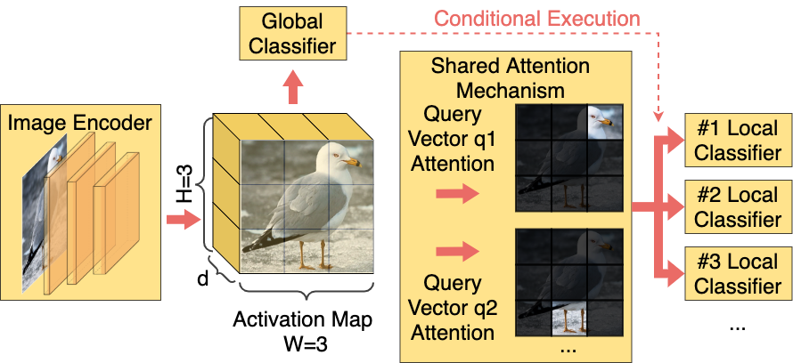
Figure 3: Local classifiers with shared attention mechanism

Local Classifier Design

Our framework is agnostic to the design choice of the local classifiers. Any design could be plugged into ALICE. We provide a default design as follows. Ideally, each local classifier should learn which semantic segments to focus and how to detect them. Since different local classifier might need to detect the same semantic segments (e.g., bill), the knowledge of detecting semantic segments could be shared among all local classifiers. Therefore, we introduce a shared attention mechanism, which is parameterized using $M$ learnable latent attention queries $q_{1},q_{2},...,q_{M}\in\mathbb{R}^{d}$ that represent $M$ different latent semantic segments. To keep our design general, we do not bind each latent attention queries to any concrete semantic segments (e.g., we do not assign binding like $q_{1}$ to “bill”) and these queries are trained in a weakly-supervised manner. Following Lin et al. (2015); Hu and Qi (2019), we view the activation map $\phi(x)\in\mathbb{R}^{H\times W\times d}$ of each image $x$ as $H\times W$ attention keys $k_{1},...,k_{H\times W}\in\mathbb{R}^{d}$. We compute the attention by:

$$Q={\left[\begin{array}[]{c}q_{1}^{T}\\ ...\\ q_{M}^{T}\end{array}\right]},K=V={\left[\begin{array}[]{c}k_{1}^{T}\\ ...\\ k_{H\times W}^{T}\end{array}\right]}$$

$$A=\mathrm{Attention}(Q,K,V)=\mathrm{softmax}(\frac{QK^{T}}{\sqrt{d}})V$$

Where $Q\in\mathbb{R}^{M\times d}$, $K=V\in\mathbb{R}^{(H\times W)\times d}$. Each row in the attention output matrix $A\in\mathbb{R}^{M\times d}$ is the attention output for each attention query $q_{i}$, which is a descriptor of the $i^{th}$ latent semantic segments. After the shared attention mechanism, each local classifier applies a private fully-connected layer on $\mathrm{flattened}(A)$ to make predictions. Each local classifier could ignore irrelevant semantic segments by simply setting the corresponding weights in its fully-connected layer to zero.

Implementation

Our image encoder $\phi$ could be any off-the-shelf visual backbone model and we use Inception v3 Szegedy et al. (2016). We implement our semantic parser on top of the Python-based SippyCup Liang and Potts (2015) following previous work Hancock et al. (2018). Our framework could support applications in other languages by changing a semantic parser for corresponding languages. We provide more details in Appendix.

5 Bird Species Classification Task

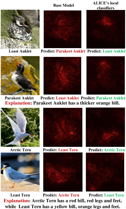
Figure 4: Saliency maps visualization. Guided by expert explanations, ALICE learn to focus on the discriminating semantic segments and make the correct prediction.

Dataset

We use the CUB-200-2011 dataset Wah et al. (2011), which contains $11,788$ images for $200$ species of North American birds. We randomly sample $25$ bird species due to limited access to expert query budget. Following Vedantam et al. (2017), We make sure that each sampled species has one or more confusing species from the same subfamilia so that they are challenging to classify. In addition, each image in the CUB data-set is also annotated with the locations of $15$ semantic segments (e.g., “bill”, “eye”). We use these location annotations to crop training image patches based on the explanations. We do not use any location annotation during testing. More details are provided in the Appendix, including the list of $25$ sampled species. We experiment with a low-resource setting with only $15$ images per bird species.

We employ an amateur bird watcher as the domain expert since we do not expect general MTurk workers to have enough domain expertise. To further ensure the annotation quality, our domain expert checks the professional birding field guide   before writing each explanation. We ask the expert, “How would you differentiate bird species $P$ and bird species $Q$?”. In total, we collect $67$ contrastive natural language explanations (avg. length $18.45$ words). We collect the explanations in an on-demand manner because our class-based active learning is empirically insensitive to the change of random seeds and hyper-parameters. Our semantic parser identifies $2.36$ semantic segments per explanation on average. In each experiment, we conduct $k=4$ rounds of expert queries, with a query budget $b=3$ for each round.

Discussion on CUB Description Dataset

The CUB description dataset collects descriptions of visual appearance for each image rather than explanations of why the bird in the image belongs to a certain class Reed et al. (2016); Hendricks et al. (2016). For example, an image with a Ring-billed gull has the description: “This is a white bird with a grey wing and orange eyes and beak.” However, this description also fits perfectly with a California gull (Figure 1). So the crowd-sourced descriptions in the CUB description dataset is not ideal to support classification. We collected expert explanations: “Ring-billed gull has a bill with a black ring near the tip while California gull has a red spot near the tip of lower mandible.” to improve classification data efficiency. In addition, we also conducted experiments to incorporate CUB descriptions (5 sentences per image), but we did not find improved performance in our setting.

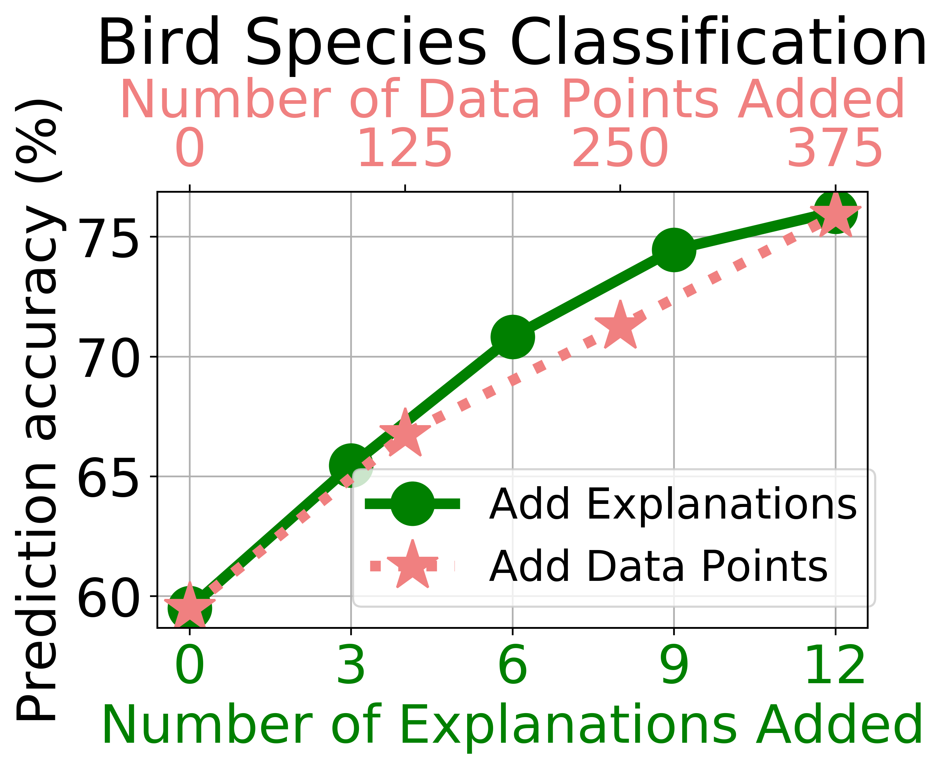
Figure 5: Comparing the performance gain of adding contrastive natural language explanations and adding training data points on bird species’ prediction accuracy. Empirically, adding $1$ explanation leads to similar performance gain as adding $30$ labeled training data points.

Model Ablations and Metrics

We compare ALICE to its several ablations (Table 2) and evaluate the performance on the test set. We report classification accuracy on species as well as subfamilia. For subfamilia accuracy, a prediction is counted as correct as long as the predicted species’ subfamilia is the same as the labeled species’ subfamilia. (1) Base(Inception v3) fine-tunes the pre-trained Inception v3 to perform a flat-$25$ way classification. (2) ALICE w/o Grounding copies the final neural architecture from ALICE but does not have access to the discriminating semantic segments ($\S$ 4.3). (3) ALICE w/o Hierarchy has the same neural architecture as (1) but has access to the discriminating semantic segments. (4) ALICE w/ Random Grounding has the semantic segments that are randomly sampled. (5) ALICE w/ Random Pairs replaces class-based active learning with randomly selected class pairs. The randomly selected class pairs are used to query experts and change the learning model’s neural architecture. (9-12) ALICE $i^{th}$ round shows ALICE’s performance after the $i^{th}$ round of expert queries. (6-8) RandomSampling + $x\%$ extra data augments (1) with $x\%$ extra training data points.

No.	Model	Accuracy (%)
		species	subfamilia
(1)	Base(Inception v3)	59.51	86.50
(2)	ALICE w/o Grounding	66.47	87.95
(3)	ALICE w/o Hierarchy	59.22	86.94
(4)	ALICE w/ Random Ground	64.44	87.52
(5)	ALICE w/ Random Pairs	42.67	75.33
(6)	RandomSampling + $33\%$ extra data	66.76	88.39
(7)	RandomSampling + $66\%$ extra data	71.26	91.00
(8)	RandomSampling + $100\%$ extra data	75.91	91.58
(9)	ALICE ($1^{st}$ round)	65.46	86.07
(10)	ALICE ($2^{nd}$ round)	70.83	89.84
(11)	ALICE ($3^{rd}$ round)	74.46	91.00
(12)	ALICE ($4^{th}$ round)	76.05	91.87

Table 2: Test accuracy comparison among variants of ALICE on the bird species classification task.

Results

Our first takeaway is that incorporating contrastive natural language explanations is more data-efficient than adding extra training data points. Figure 5 visualizes the performance gain of adding explanations and adding data points. ((6-12) in Table 2). As shown in Figure 5, adding $1$ explanation leads to the same amount of performance gain of adding $30$ labeled data points. For example, adding $12$ explanations (ALICE ($4^{th}$ round), $76.05\%$) achieves comparable performance gain of adding $375$ training images (RandomSampling + $100\%$ extra data, $75.91\%$). We note that writing one explanation for an expert is typically faster than labeling 15-30 examples. As an estimate, Zhou et al. (2020); Hancock et al. (2018); Zaidan and Eisner (2008) perform user study and find that collecting natural language explanations is only twice as costly as collecting labels for their tasks. Our experiment shows that adding $1$ explanation leads to similar performance gain as adding $30$ labeled training data points, yielding a $6\times$ speedup.

Our second takeaway is that both the grounding of explanations’ semantics and the hierarchical neural architecture improves classification performance a lot. Removing the grounded training image patches degrades ALICE’s performance (ALICE w/o Grounding, $66.47\%$). Substituting the discriminating semantic segments’ image patches with other semantic segments’ patches leads to worse performance (ALICE w/ Random Grounding, $64.44\%$). The hierarchical neural architecture is also important. As shown in Table 2, a baseline model augmented with hierarchical classification (ALICE w/o Grounding, $66.74\%$) outperforms the flat $C$ way classification (Base(Inception v3), $59.51\%$). Similarly, removing the hierarchical neural architecture from ALICE drops the performance a lot (ALICE w/o Hierarchy, $59.22\%$ v.s. ALICE ($4^{th}$ round), $76.05\%$). ALICE morphs the neural architecture based on class-based active learning ($\S$ 4.2). If we replace class-based active learning with a random selection of class pairs, ALICE learns a bad model structure that leads to reduced performance (ALICE w/ Random Pairs, $42.67\%$).

No.	Method	Species Acc (%)
		+33% data	+66% data
(1)	RandomSampling	66.76	71.26
(2)	CoreSet	68.06	73.09
(3)	LeastConfidence	67.34	71.94
(4)	MarginSampling	66.04	70.36
(5)	EntropySampling	66.91	72.52
(6)	BALDdropout	66.33	71.65

Table 3: Instance-based active learning baselines on the bird species classification task. We note that ALICE ($4^{th}$ round, Acc $76.05\%$) in Table 2 (12) outperforms all instance-based active learning baselines with $66\%$ extra training data (Acc $70.36\%$-$73.09\%$).

Additional Experiments

Table 3 shows our experiments with several common instance-based active learning baselines. We show the test accuracy of adding $33\%$ extra training data (i.e., $125$ extra data points) and adding $66\%$ extra training data (i.e., $250$ extra data points) using the instance-based active learning baselines. In this case, we observe that ALICE with 12 explanations (Accuracy $76.05\%$, Table 2 (12)) outperforms all instance-based active learning baselines with 250 extra data points(Accuracy $70.36\%$-$73.09\%$, Table 3). We delay the combination of instance-based active learning and our class-based active learning as future work. To testify whether ALICE could work robustly with smaller amount of training data, we present an experiment on CUB starting with as few as $5$ images per species. ALICE with $12$ explanations ($k=4$, $b=3$) improves the accuracy of the base model from $49.76\%$ to $62.80\%$, outperforming the base model with $15$ images per class (Accuracy $59.51\%$, Table 2).

Visualization

We show how the explanations help the learning model as shown in Figure 4. We visualize the saliency maps Simonyan et al. (2014) corresponding to the correct class on four example images. As shown in Figure 4, the base model does not know which semantic segments to focus and makes wrong predictions. In contrast, ALICE’s local classifiers obtain knowledge from the expert explanations and successfully learns to focus on the discriminating semantic segments to make the correct predictions.

6 Social Relationship Classification Task

No.	Model	Accuracy (%)
		relation	domain
(1)	Base(Inception v3)	33.67	45.39
(2)	ALICE w/ Random Ground	27.20	42.52
(3)	ALICE w/ Random Pairs	22.94	35.29
(4)	RandomSampling + $20\%$ extra data	34.91	46.51
(5)	RandomSampling + $40\%$ extra data	36.28	46.63
(6)	ALICE ($1^{st}$ round)	35.29	47.13
(7)	ALICE ($2^{nd}$ round)	36.41	47.38

Table 4: Test accuracy comparison among variants of ALICE on the social relationship classification task.

Dataset

We also evaluate ALICE on the People in Photo Album Relation dataset  Zhang et al. (2015); Sun et al. (2017). An example is shown in Figure 6. The dataset was originally collected from Flickr photo albums and involves 5 social domains and 16 social relations. We focus on the images that have only two people since handling more than two people requires task-specific neural architecture. The details of dataset pre-processing are included in Appendix. After pre-processing, we obtain $1,679$ training images and $802$ testing images. We experiment with a low-resource setting with $15\%$ of the remaining training images (i.e., $264$ images). We obtain explanations by converting the knowledge graph collected by Wang et al. (2018) into a parsed format. The semantic segments here are contextual objects like soccer. The knowledge graph contains heuristics to distinguish social relations by the occurrence of contextual objects (e.g., “soccer” for sports v.s. colleagues). We use a faster-RCNN-based object detector Ren et al. (2017) trained on the COCO dataset Lin et al. (2014) to localize the semantic segments (contextual objects) during training. The object detector is not used during testing. We set rounds of expert queries $k=2$ and the query budget $b=4$.

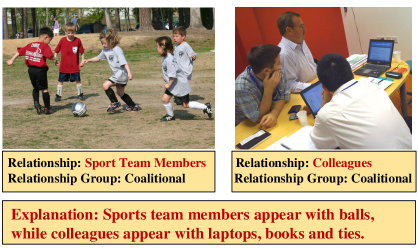
Figure 6: Examples of social relationship classification. Explanations are reconstructed from Wang et al. (2018)

Results

We compare ALICE to its several ablations (Table 4) and evaluate the performance on the testing set. We report classification accuracy on social relationships as well as social domains. We observe similar benefits of incorporating explanations to ALICE as in the bird species classification task. As shown in Table 4, the base model with $40\%$ extra training data (i.e., $105$ images) still slightly underperforms ALICE with $8$ explanations (RandomSampling + $40\%$ extra data, $36.28\%$ v.s. ALICE ($2^{nd}$ round), $36.41\%$). As shown in Figure 7, adding $1$ explanation leads to similar performance gain as adding $13$ labeled training data points. Our ablation experiment also confirms the importance of class-based active learning. If we replace class-based active learning with a random selection of class pairs, ALICE learns a bad model structure that leads to reduced performance (ALICE w/ Random Pairs, $22.94\%$). The performance drop in domain accuracy is also significant. We suspect it is because the bad model structure confuses the global classifier a lot. If the global classifier calls a wrong local classifier, the local classifier is forced to make a prediction on such a out-of-distribution data. In addition, our ablation experiment also verify the importance of having knowledge beyond having the localization model. Substituting the discriminating semantic segments’ image patches with other semantic segments’ patches leads to worse performance (ALICE w/ Random Grounding, $27.20\%$). One reason is that there are many objects in each image. Under our low resource setting, learning on the image patches of random semantic segments may make the model to latch on to sample-specific artifacts in the training images, which leads to poor generalization.

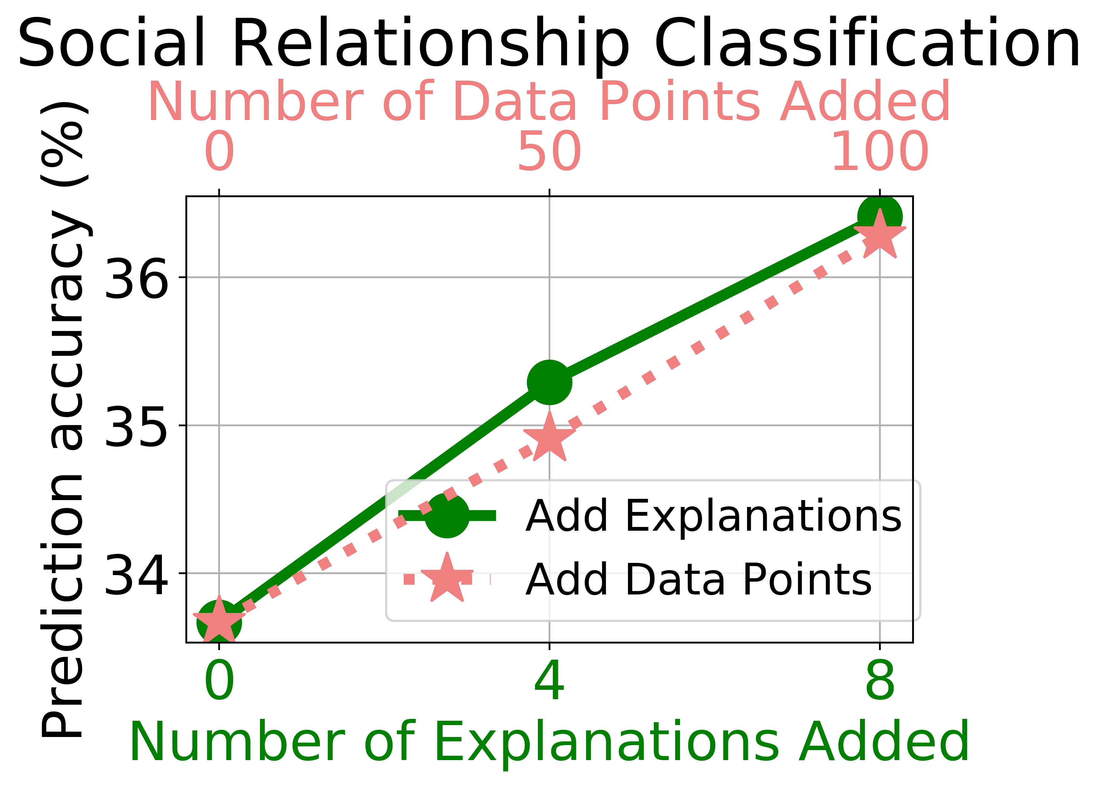
Figure 7: Comparing the performance gain of adding contrastive natural language explanations and adding training data points on social relationship classification.

7 Conclusion

We propose an expert-in-the-loop training framework ALICE to utilize contrastive natural language explanations to improve a learning algorithm’s data efficiency. We extend the concept of active learning to class-based active learning for choosing the most informative query pair. We incorporate the extracted knowledge from expert natural language explanation by changing our algorithm’s neural network structure. Our experiments on two visual recognition tasks show that incorporating natural language explanations is far more data-efficient than adding extra training data. In the future, we plan to examine the hierarchical classification architecture’s potential for reducing computational runtime.

Appendix

Additional Implementation Details

We use Inception v3 Szegedy et al. (2016) as our image encoder $\phi$. The global pooling layer $g_{pool}$ is a global average pooling layer. The input image size is $(448,448)$. We implement our model in PyTorch. We implement the shared attention infrastructure of fine-grained classifiers by noting that calculating $QK^{T}$ is equivalent to an efficient $1\times 1\times d$ convolution on the activation map $\phi(x)\in\mathbb{R}^{H\times W\times d}$, with $M$ latent attention queries as $M$ convolutional kernels. We use the same hyper-parameters for both datasets. We adopt Inception v3 Szegedy et al. (2016) as the backbone and choose Mix6e layer as the activation map. We tune the hyper-parameters on the unused training images. We train the models using Stochastic Gradient Descent (SGD) with the momentum of $0.9$, weight decay of $1e-5$. We decay the learning rate of each parameter group by $0.9$ every $2$ epochs using torch.optim.lr_scheduler.StepLR. The global pooling $g$ is a global average pooling layer. We set $M$ the number of learnable latent attention queries to $6$. The total number of parameters of our model is $15,114,476$. The training time for our approach is less than $20$ minutes since our resource constraint setting has a limited amount of training data. Unlike previous active learning on data-points, our class-based active learning is empirically insensitive to the change of random seeds and hyper-parameter (e.g., batch size). Therefore, we could collect the explanations in an on-demand manner.

Bird Species Classification Dataset

We adopt the random sampling method in  Vedantam et al. (2017), to make sure that the sampled species are challenging to classify. The sampling method is based on birds’ biological hierarchy Barz and Denzler (2020) from Wikispecies. The $25$ randomly sampled bird species are: Crested Auklet, Least Auklet, Parakeet Auklet, Tropical Kingbird, Gray Kingbird, Belted Kingfisher, Green Kingfisher, Pied Kingfisher, Ringed Kingfisher, Scarlet Tanager, Summer Tanager, Brown Thrasher, Sage Thrasher, California Gull, Heermann Gull, Ivory Gull, Ring billed Gull, Black capped Vireo, Blue headed Vireo, White eyed Vireo, Yellow throated Vireo, Artic Tern, Black Tern, Caspian Tern, Least Tern.

Saliency Map Visualization

We use the techniques in Simonyan et al. (2014) to visualze the saliency map. A saliency map tells us the degree to which each pixel in the image affects the classification score for that image. To compute it, we compute the gradient of the unnormalized score corresponding to the correct class (which is a scalar) with respect to the pixels of the image. If the image has shape $(3,H,W)$ then this gradient will also have shape $(3,H,W)$; for each pixel in the image, this gradient tells us the amount by which the classification score will change if the pixel changes by a small amount. To compute the saliency map, we take the absolute value of this gradient, then take the maximum value over the $3$ input channels; the final saliency map thus has shape $(H,W)$ and all entries are nonnegative.

Social Relationship Classification Dataset

PIPA-Relation dataset Sun et al. (2017) is built on PIPA dataset Zhang et al. (2015). We exclude the images with more than two people since it requires task-specific neural architecture. Since we have annotations of people pairs for each image, we could easily identify and remove images with more than two people. However, the dataset becomes heavily unbalanced after this step since images of certain relationships tend to have less people. To tackle this issue, we truncate the classes that have more than $200$ training images left to $200$ training images. Similarly, we truncate the classes that have more than $100$ testing images left to $100$ testing images. We finally get $1679$ training images and $802$ testing images.

References

- Abid et al. (2018) Abubakar Abid, Martin J Zhang, Vivek K Bagaria, and James Zou. 2018. Exploring patterns enriched in a dataset with contrastive principal component analysis. Nature communications, 9(1):1–7.
- Andreas et al. (2018) Jacob Andreas, Dan Klein, and Sergey Levine. 2018. Learning with latent language. In NAACL-HLT, pages 2166–2179. Association for Computational Linguistics.
- Barz and Denzler (2020) Björn Barz and Joachim Denzler. 2020. Deep learning on small datasets without pre-training using cosine loss. In WACV, pages 1360–1369. IEEE.
- Biederman (1987) Irving Biederman. 1987. Recognition-by-components: a theory of human image understanding. Psychological review, 94(2):115.
- Chen et al. (2020) Lingjiao Chen, Matei Zaharia, and James Zou. 2020. Frugalml: How to use ML prediction apis more accurately and cheaply. CoRR, abs/2006.07512.
- Chen et al. (2014) Xianjie Chen, Roozbeh Mottaghi, Xiaobai Liu, Sanja Fidler, Raquel Urtasun, and Alan L. Yuille. 2014. Detect what you can: Detecting and representing objects using holistic models and body parts. In CVPR, pages 1979–1986. IEEE Computer Society.
- Chin-Parker and Cantelon (2017) Seth Chin-Parker and Julie Cantelon. 2017. Contrastive constraints guide explanation-based category learning. Cognitive science, 41(6):1645–1655.
- Feng et al. (2019) Zunlei Feng, Weixin Liang, Daocheng Tao, Li Sun, Anxiang Zeng, and Mingli Song. 2019. Cu-net: Component unmixing network for textile fiber identification. Int. J. Comput. Vis., 127(10):1443–1454.
- Hancock et al. (2018) Braden Hancock, Paroma Varma, Stephanie Wang, Martin Bringmann, Percy Liang, and Christopher Ré. 2018. Training classifiers with natural language explanations. In ACL (1), pages 1884–1895. Association for Computational Linguistics.
- He and Peng (2017) Xiangteng He and Yuxin Peng. 2017. Fine-grained image classification via combining vision and language. In CVPR, pages 7332–7340. IEEE Computer Society.
- Hendricks et al. (2016) Lisa Anne Hendricks, Zeynep Akata, Marcus Rohrbach, Jeff Donahue, Bernt Schiele, and Trevor Darrell. 2016. Generating visual explanations. In ECCV (4), volume 9908 of Lecture Notes in Computer Science, pages 3–19. Springer.
- Hu and Qi (2019) Tao Hu and Honggang Qi. 2019. See better before looking closer: Weakly supervised data augmentation network for fine-grained visual classification. CoRR, abs/1901.09891.
- Krishna et al. (2017) Ranjay Krishna, Yuke Zhu, Oliver Groth, Justin Johnson, Kenji Hata, Joshua Kravitz, Stephanie Chen, Yannis Kalantidis, Li-Jia Li, David A. Shamma, Michael S. Bernstein, and Li Fei-Fei. 2017. Visual genome: Connecting language and vision using crowdsourced dense image annotations. Int. J. Comput. Vis., 123(1):32–73.
- Liang and Potts (2015) Percy Liang and Christopher Potts. 2015. Bringing machine learning and compositional semantics together. Annu. Rev. Linguist., 1(1):355–376.
- Liang et al. (2019) Weixin Liang, Youzhi Tian, Chengcai Chen, and Zhou Yu. 2019. MOSS: end-to-end dialog system framework with modular supervision. CoRR, abs/1909.05528.
- Liang et al. (2020) Weixin Liang, James Zou, and Zhou Yu. 2020. Beyond user self-reported likert scale ratings: A comparison model for automatic dialog evaluation. In ACL, pages 1363–1374. Association for Computational Linguistics.
- Lin et al. (2014) Tsung-Yi Lin, Michael Maire, Serge J. Belongie, James Hays, Pietro Perona, Deva Ramanan, Piotr Dollár, and C. Lawrence Zitnick. 2014. Microsoft COCO: common objects in context. In ECCV (5), volume 8693 of Lecture Notes in Computer Science, pages 740–755. Springer.
- Lin et al. (2015) Tsung-Yu Lin, Aruni RoyChowdhury, and Subhransu Maji. 2015. Bilinear CNN models for fine-grained visual recognition. In ICCV, pages 1449–1457. IEEE Computer Society.
- Lipton (1990) Peter Lipton. 1990. Contrastive explanation. Royal Institute of Philosophy Supplements, 27:247–266.
- Lombrozo (2006) Tania Lombrozo. 2006. The structure and function of explanations. Trends in cognitive sciences, 10(10):464–470.
- Luo and Hauskrecht (2017) Zhipeng Luo and Milos Hauskrecht. 2017. Group-based active learning of classification models. In FLAIRS Conference, pages 92–97. AAAI Press.
- Mailthody et al. (2019) Vikram Sharma Mailthody, Zaid Qureshi, Weixin Liang, Ziyan Feng, Simon Garcia De Gonzalo, Youjie Li, Hubertus Franke, Jinjun Xiong, Jian Huang, and Wen-Mei Hwu. 2019. Deepstore: In-storage acceleration for intelligent queries. In MICRO, pages 224–238. ACM.
- Miller (2019) Tim Miller. 2019. Explanation in artificial intelligence: Insights from the social sciences. Artificial Intelligence, 267:1–38.
- Mittelstadt et al. (2019) Brent D. Mittelstadt, Chris Russell, and Sandra Wachter. 2019. Explaining explanations in AI. In FAT, pages 279–288. ACM.
- Mu et al. (2020) Jesse Mu, Percy Liang, and Noah Goodman. 2020. Shaping visual representations with language for few-shot classification. In Proceedings of the 58th Annual Meeting of the Association for Computational Linguistics.
- Murty et al. (2020) Shikhar Murty, Pang Wei Koh, and Percy Liang. 2020. Expbert: Representation engineering with natural language explanations. CoRR, abs/2005.01932.
- Reed et al. (2016) Scott E. Reed, Zeynep Akata, Honglak Lee, and Bernt Schiele. 2016. Learning deep representations of fine-grained visual descriptions. In CVPR, pages 49–58. IEEE Computer Society.
- Ren et al. (2017) Shaoqing Ren, Kaiming He, Ross B. Girshick, and Jian Sun. 2017. Faster R-CNN: towards real-time object detection with region proposal networks. IEEE Trans. Pattern Anal. Mach. Intell., 39(6):1137–1149.
- Sener and Savarese (2018) Ozan Sener and Silvio Savarese. 2018. Active learning for convolutional neural networks: A core-set approach. In ICLR (Poster). OpenReview.net.
- Settles (2009) Burr Settles. 2009. Active learning literature survey. Technical report, University of Wisconsin-Madison Department of Computer Sciences.
- Settles (2011) Burr Settles. 2011. From theories to queries: Active learning in practice. In Active Learning and Experimental Design workshop In conjunction with AISTATS 2010, pages 1–18.
- Simonyan et al. (2014) Karen Simonyan, Andrea Vedaldi, and Andrew Zisserman. 2014. Deep inside convolutional networks: Visualising image classification models and saliency maps. In ICLR (Workshop Poster).
- Smith (2003) Linda B Smith. 2003. Learning to recognize objects. Psychological Science, 14(3):244–250.
- Srivastava et al. (2017) Shashank Srivastava, Igor Labutov, and Tom M. Mitchell. 2017. Joint concept learning and semantic parsing from natural language explanations. In EMNLP, pages 1527–1536. Association for Computational Linguistics.
- Sun et al. (2017) Qianru Sun, Bernt Schiele, and Mario Fritz. 2017. A domain based approach to social relation recognition. In CVPR, pages 435–444. IEEE Computer Society.
- Szegedy et al. (2015) Christian Szegedy, Wei Liu, Yangqing Jia, Pierre Sermanet, Scott E. Reed, Dragomir Anguelov, Dumitru Erhan, Vincent Vanhoucke, and Andrew Rabinovich. 2015. Going deeper with convolutions. In CVPR, pages 1–9. IEEE Computer Society.
- Szegedy et al. (2016) Christian Szegedy, Vincent Vanhoucke, Sergey Ioffe, Jonathon Shlens, and Zbigniew Wojna. 2016. Rethinking the inception architecture for computer vision. In CVPR, pages 2818–2826. IEEE Computer Society.
- Vedantam et al. (2017) Ramakrishna Vedantam, Samy Bengio, Kevin Murphy, Devi Parikh, and Gal Chechik. 2017. Context-aware captions from context-agnostic supervision. In CVPR, pages 1070–1079. IEEE Computer Society.
- Wah et al. (2011) C. Wah, S. Branson, P. Welinder, P. Perona, and S. Belongie. 2011. The Caltech-UCSD Birds-200-2011 Dataset. Technical Report CNS-TR-2011-001, California Institute of Technology.
- Wang et al. (2018) Zhouxia Wang, Tianshui Chen, Jimmy S. J. Ren, Weihao Yu, Hui Cheng, and Liang Lin. 2018. Deep reasoning with knowledge graph for social relationship understanding. In IJCAI, pages 1021–1028. ijcai.org.
- Xiao et al. (2014) Tianjun Xiao, Jiaxing Zhang, Kuiyuan Yang, Yuxin Peng, and Zheng Zhang. 2014. Error-driven incremental learning in deep convolutional neural network for large-scale image classification. In ACM Multimedia, pages 177–186. ACM.
- Yan et al. (2015) Zhicheng Yan, Hao Zhang, Robinson Piramuthu, Vignesh Jagadeesh, Dennis DeCoste, Wei Di, and Yizhou Yu. 2015. HD-CNN: hierarchical deep convolutional neural networks for large scale visual recognition. In ICCV, pages 2740–2748. IEEE Computer Society.
- Zaidan and Eisner (2008) Omar Zaidan and Jason Eisner. 2008. Modeling annotators: A generative approach to learning from annotator rationales. In EMNLP, pages 31–40. ACL.
- Zhang et al. (2015) Ning Zhang, Manohar Paluri, Yaniv Taigman, Rob Fergus, and Lubomir D. Bourdev. 2015. Beyond frontal faces: Improving person recognition using multiple cues. In CVPR, pages 4804–4813. IEEE Computer Society.
- Zhou et al. (2020) Wenxuan Zhou, Hongtao Lin, Bill Yuchen Lin, Ziqi Wang, Junyi Du, Leonardo Neves, and Xiang Ren. 2020. NERO: A neural rule grounding framework for label-efficient relation extraction. In WWW, pages 2166–2176. ACM / IW3C2.
- Zou et al. (2015) James Y Zou, Kamalika Chaudhuri, and Adam Tauman Kalai. 2015. Crowdsourcing feature discovery via adaptively chosen comparisons. arXiv preprint arXiv:1504.00064.
- Zou et al. (2013) James Y Zou, Daniel J Hsu, David C Parkes, and Ryan P Adams. 2013. Contrastive learning using spectral methods. In Advances in Neural Information Processing Systems, pages 2238–2246.