Abstract

A $(m+3)$-dimensional Einstein-Gauss-Bonnet gravitational model including the Gauss-Bonnet term and the cosmological term $\Lambda$ is considered. Exact solutions with exponential time dependence of two scale factors, governed by two Hubble-like parameters $H>0$ and $h\neq H$, corresponding to factor spaces of dimensions $m>2$ and $l=2$, respectively, are found. Under certain restrictions on $x=h/H$, the stability of the solutions in a class of cosmological solutions with diagonal metrics is proved. A subclass of solutions with small enough variation of the effective gravitational constant $G$ is considered and the stability of all solutions from this subclass is shown.

Keywords: Gauss-Bonnet, variation of G, accelerated expansion of the Universe

1 Introduction

This paper is a continuation of our previous work [1] devoted to cosmological solutions with two factor-spaces in the Einstein-Gauss-Bonnet (EGB) gravitational model in $D$ dimensions, which contains the so-called Gauss-Bonnet term and cosmological term $\Lambda$. Such model may be also referred as EGB$\Lambda$ one. The Gauss-Bonnet term appeared in low-energy limit of certain effective string action [3]-[5]. It also appears in the action of Einstein-Lovelock (EL) gravity [6, 7] for $D>4$ as a first non-trivial addition (quadratic in curvature) to the Einstein-Hilbert action (with a $\Lambda$-term).

Currently, there exists a certain interest to EGB and EL gravitational models and its extensions, see [8]-[27] and refs. therein. The main motivation for this activity is in possible explanation of supernovae (type Ia) observational data [29, 30, 31], which tell us about accelerating expansion of the Universe. There exists also a considerable interest in studying of black-hole solutions in EGB and EL theories, see refs. [32]-[37].

Here we study the cosmological solutions with exponential dependence of scale factors upon synchronous time variable and find a new class of solutions with two scale factors, governed by two Hubble-like parameters $H>0$ and $h$, which correspond to factor spaces of dimensions $m>2$ and $2$, respectively, ($D=1+m+2$) and obey relations: $mH+2h\neq 0$ and $H\neq h$. Any of these solutions describes an exponential expansion of $3$-dimensional subspace with Hubble parameter $H>0$ [38]. Here, as in our previous paper [1], we use the Chirkov-Pavluchenko-Toporensky trick of reducing the set of polynomial equations on parameters $H$ and $h$ from ref. [20]. By using results of refs. [25] we show that the solutions are stable when certain restrictions on ratio $h/H$ are imposed. Here the stability of the solutions is understood such that the allowed perturbations of the metric do not output the solutions from the class of cosmological solutions with diagonal metrics.

We also study solutions with a small enough variation of the effective gravitational constant $G$ in Jordan frame [39, 40] which obey the restrictions on $G$-dot from ref. [41]. We show that these solutions are stable.

Earlier in Ref. [1] we were dealing with exponential cosmological solutions in the EGB model (with a $\Lambda$-term) with two non-coinciding Hubble-like parameters $H>0$ and $h$ obeying $S_{1}=mH+lh\neq 0$ and corresponding to $m$- and $l$-dimensional factor spaces with $m>2$ and $l>2$, respectively. In this case we have found two sets of solutions obeying: a) $\alpha>0$, $\Lambda<\alpha^{-1}\lambda_{+}(m,l)$ and b) $\alpha<0$, $\Lambda>|\alpha|^{-1}\lambda_{-}(m,l)$, with $\lambda_{\pm}(m,l)>0$. Here $\alpha=\alpha_{2}/\alpha_{1}$, where $\alpha_{1}$ and $\alpha_{2}$ are two non-zero constants of the model. We show, that in the case $m>2$, $l=2$, $\alpha>0$ the “spectrum” of allowed values for $\Lambda$ is unbounded from the top and the bottom and the ratio $x=h/H$ is unbounded from the bottom ($-\infty<x<x_{*}$), while in the case $m>2$, $l>2$, $\alpha>0$ [1] the set of allowed values for $\Lambda$ is bounded from the top and set of ratios $x=h/H$ is bounded ($x_{-}<x<x_{+}<0$). From matematical point of view we have here a more simple task since for $m>2$, $l=2$ the polynomial master equation for $x$ is of third order while in the case $m>2$, $l>2$ it is generically of fourth order [1]. The solution to the master equation is presented in Appendix.

2 The cosmological model

We start with the action

$$S=\int_{M}d^{D}z\sqrt{|g|}\{\alpha_{1}(R[g]-2\Lambda)+\alpha_{2}{\cal L}_{2}[g]\},$$ (2.1)

where $g=g_{MN}dz^{M}\otimes dz^{N}$ is the metric on the manifold $M$, ${\dim M}=D$, $|g|=|\det(g_{MN})|$, $\Lambda$ is the cosmological term, $R[g]$ is scalar curvature,

$${\cal L}_{2}[g]=R_{MNPQ}R^{MNPQ}-4R_{MN}R^{MN}+R^{2}$$

is the Gauss-Bonnet term and $\alpha_{1}$, $\alpha_{2}$ are nonzero constants of the model.

Here we deal with the manifold

$$M={\mathbb{R}}\times M_{1}\times\ldots\times M_{n}$$ (2.2)

and the metric

$$g=-dt\otimes dt+\sum_{i=1}^{n}B_{i}e^{2v^{i}t}dy^{i}\otimes dy^{i},$$ (2.3)

where $B_{i}>0$ are constants, $i=1,\dots,n$. In (2.2) $M_{1},\dots,M_{n}$ are one-dimensional manifolds, either ${\mathbb{R}}$ or $S^{1}$, and $n>3$.

The equations of motion for the action (2.1) and the metric (2.3) read [24, 28]

$$G_{ij}v^{i}v^{j}+2\Lambda-\alpha G_{ijkl}v^{i}v^{j}v^{k}v^{l}=0,$$ (2.4)

$$\left[2G_{ij}v^{j}-\frac{4}{3}\alpha G_{ijkl}v^{j}v^{k}v^{l}\right]\sum_{k=1}^{n}v^{k}-\frac{2}{3}G_{sj}v^{s}v^{j}+\frac{8}{3}\Lambda=0,$$ (2.5)

$i=1,\ldots,n$, where $\alpha=\alpha_{2}/\alpha_{1}$. Here as in refs. [16, 17] we use the notations

$$G_{ij}=\delta_{ij}-1,\qquad G_{ijkl}=G_{ij}G_{ik}G_{il}G_{jk}G_{jl}G_{kl}.$$ (2.6)

For $n>3$ ($D>4$) we get a set of forth-order polynomial equations.

In ref. [19] an isotropic solution $v^{1}=\ldots=v^{n}=H$ was obtained for $\Lambda\neq 0$, $\alpha<0$, see also ref. [25].

It was proved in ref. [25] that there are no more than three different numbers among $v^{1},\dots,v^{n}$ obeying $\sum_{i=1}^{n}v^{i}\neq 0$.

3 Solutions with two Hubble-like parameters

Here we deal with solutions to equations (2.4), (2.5) governed by two parameters:

$$v=(\underbrace{H,H,H}_{``our"\ space},\underbrace{\overbrace{H,\ldots,H}^{m-3},h,h}_{internal\ space}).$$ (3.1)

The Hubble-like parameter $H$ corresponds to $m$-dimensional factor space with $m>2$ and Hubble-like parameter $h$ corresponds to $2$-dimensional factor space.

Keeping in mind possible cosmological applications, we split the $m$-dimensional factor space into the product of two subspaces of dimensions $3$ and $m-3$, respectively, and obtain $3$–dimensional “our” space and $((m-3)+2)$-dimensional anisotropic “internal space”. For physical applications (in our epoch) the internal space should be chosen to be compact one, i.e. one should put in (2.2) $M_{4}=\ldots=M_{n}=S^{1}$, while $M_{1}=M_{2}=M_{3}={\mathbb{R}}$ and the internal scale factors corresponding to present time should be small enough in comparison with the scale factors of “our” space.

In order to describe possible accelerated expansion of a $3d$ subspace (“our Universe”) we put

$$H>0.$$ (3.2)

According to ansatz (3.1), the $m$-dimensional factor space is expanding with the Hubble parameter $H>0$, while the evolution of the $2$-dimensional factor space is driven by the Hubble-like parameter $h$.

As in our previous paper [1] we impose the following restrictions on parameters $H$ and $h$

$$mH+2h\neq 0,\qquad H\neq h.$$ (3.3)

With the ansatz (3.1) and the restrictions (3.3) imposed the relations (2.4) and (2.5) can be reduced to a set of two polynomial equations [20, 25]

$$E=mH^{2}+2h^{2}-(mH+2h)^{2}+2\Lambda$$

$$-\alpha[m(m-1)(m-2)(m-3)H^{4}$$

$$+8m(m-1)(m-2)H^{3}h+12m(m-1)H^{2}h^{2}]=0,$$ (3.4)

$$Q=(m-1)(m-2)H^{2}+2(m-1)Hh=-\frac{1}{2\alpha}.\qquad$$ (3.5)

For $m>2$ equation (3.5) implies

$$H=(-2\alpha{\cal P})^{-1/2},$$ (3.6)

where

$${\cal P}={\cal P}(x,m)=(m-1)(m-2)+2(m-1)x,$$ (3.7)

$$x=h/H,$$ (3.8)

and

$$\alpha{\cal P}<0.$$ (3.9)

Restrictions (3.3) may be written as

$$x\neq x_{d}=x_{d}(m)\equiv-m/2,\qquad x\neq x_{a}\equiv 1.$$ (3.10)

Relation (3.5) is valid only if

$${\cal P}(x,m)\neq 0.$$ (3.11)

Substituting (3.6) into (3.4) we obtain

$$\Lambda\alpha=\lambda=\lambda(x,m)\equiv\frac{1}{4}({\cal P}(x,m))^{-1}{\cal M}(x,m)\qquad$$

$$+\frac{1}{8}({\cal P}(x,m))^{-2}{\cal R}(x,m),\qquad$$ (3.12)

$${\cal M}(x,m)\equiv m+2x^{2}-(m+2x)^{2},\qquad$$ (3.13)

$${\cal R}(x,m)\equiv m(m-1)(m-2)(m-3)\qquad$$

$$+8m(m-1)(m-2)x+12m(m-1)x^{2}.\qquad$$ (3.14)

Using (3.11) we get

$$x\neq x_{*}=x_{*}(m)\equiv-(m-2)/2.\qquad$$ (3.15)

We have ($m>2$)

$$x_{*}(m)<0.$$ (3.16)

Using (3.9) and (3.12) we find

$$\Lambda=\alpha^{-1}\lambda(x,m),\qquad$$ (3.17)

where

$$x<x_{*}(m)\ {\rm for}\ \alpha>0\qquad$$ (3.18)

and

$$x>x_{*}(m)\ {\rm for}\ \alpha<0.\qquad$$ (3.19)

For $\alpha<0$ we have the following limit

$$\lim_{x\to+\infty}\lambda(x,m)=-\infty,\qquad$$ (3.20)

while for $\alpha>0$ we obtain

$$\lim_{x\to-\infty}\lambda(x,m)=+\infty.\qquad$$ (3.21)

We note that

$$\lambda(x)\sim-x/(4(m-1))$$ (3.22)

as $x\to\pm\infty$.

For $x=0$ we get (here $\alpha<0$, $m>2$)

$$\Lambda=\Lambda_{0}=\alpha^{-1}\lambda(0,m)=-\frac{m(m+1)}{8\alpha(m-1)(m-2)}>0,\qquad$$ (3.23)

and

$$H=H_{0}=(-2\alpha(m-1)(m-2))^{-1/2},\qquad h=0,$$ (3.24)

i.e. (see (2.2), (2.3)) we get the product of (a part of) $(m+1)$-dimensional de-Sitter space and $2$-dimensional Euclidean space.

“Master” equation. Rewriting eq. (3.12) we are led to a “master” equation

$$2{\cal P}(x,m){\cal M}(x,m)+{\cal R}(x,m)-8\lambda({\cal P}(x,m))^{2}=0,\qquad$$ (3.25)

which is of third order in $x$. For any $m>2$ the equation (3.25) may be readily solved in radicals, the solution is presented in Appendix A.

The behaviour of the function $\lambda(x,m)$ in the vicinity of the point $x_{*}(m)$ is desribed by the following proposition.

Proposition 1. For $m>2$,

$$\lambda(x,m)\sim B(m)(x-x_{*}(m))^{-2},$$ (3.26)

as $x\to x_{*}=x_{*}(m)$, where $B(m)=-(m(m-2))/(32(m-1))<0$ and hence

$$\lim_{x\to x_{*}}\lambda(x,m)=-\infty.$$ (3.27)

For a given $m>2$ let us analyze the behaviour of the function $\lambda(x,m)$ in $x$ for $x\neq x_{*}(m)$. First, we find the extremum points obeying $\frac{\partial}{\partial x}\lambda(x,m)=0$. We obtain

$$\frac{\partial}{\partial x}\lambda(x,m)=-f(x,m)({\cal P}(x,m))^{-3},\qquad$$ (3.28)

$$f(x,m)=(m-1)^{2}(x-1)(2x+m)(x+m-2),\qquad$$ (3.29)

$x\neq x_{*}(m)$. Using these relations we get the following extremum points

$$x_{a}=1,\qquad$$ (3.30)

$$x_{c}=x_{c}(m)\equiv-(m-2)<0,\qquad$$ (3.31)

$$x_{d}=x_{d}(m)\equiv-\frac{m}{2}<0.\qquad$$ (3.32)

For points $x_{c},x_{d}$ the following inequalities are valid

$$x_{i}(m)<x_{*}(m),\qquad$$ (3.33)

$i=c,d$ ($m>2$).

We also get

$$(1)\ x_{c}<x_{d} \text{for }m>4,$$ (3.34)

$$(2)\ x_{c}=x_{d} \text{for }m=4,$$ (3.35)

$$(3)\ x_{d}<x_{c} \text{for }m=3.$$ (3.36)

For $\lambda_{i}=\lambda(x_{i},m)$, $i=a,c,d$, we obtain

$$\lambda_{a}=-\frac{(m+1)(m+2)}{8(m-1)m}<0,$$ (3.38)

$$\lambda_{c}=\frac{3m^{2}-13m+16}{8(m-2)(m-1)}>0,$$ (3.39)

and

$$\lambda_{d}=\frac{m(m+2)}{32(m-1)}>0$$ (3.40)

for all $m>2$.

We also get

$$\lambda_{d}-\lambda_{c}=\frac{(m-4)^{3}}{32(m-2)(m-1)}$$ (3.41)

for $m>2$. By using this relation we obtain

$$\lambda_{d}-\lambda_{c}\begin{cases}>0,\ \text{if }m>4,\\ =0,\ \text{if }m=4,\\ <0,\ \text{if }m=3.\end{cases}$$ (3.42)

Let us denote by $n(\Lambda,\alpha)$ the number of solutions (in $x$) of the equation $\Lambda\alpha=\lambda(x,m)$. We calculate $n(\Lambda,\alpha)$ by using unequalities for points of extremum $x_{i}$ and $\lambda_{i}$ ($i=c,d$) presented above and relations (3.20), (3.21), (3.27), (3.28) and (3.29).

First, we start with the case $\alpha>0$ and $x<x_{*}$.

(1) $m>4$. We get $x_{c}<x_{d}$ and $\lambda_{c}<\lambda_{d}$. Here $x_{d}$ is point of local maximum and $x_{c}$ is a point of local minimum. We obtain

$$n(\Lambda,\alpha)=\begin{cases}1,\ \Lambda\alpha\geq\lambda_{d},\\ 3,\ \lambda_{c}<\Lambda\alpha<\lambda_{d},\\ 2,\ \Lambda\alpha=\lambda_{c},\\ 1,\ \Lambda\alpha<\lambda_{c}.\end{cases}$$ (3.43)

Here and in what follows we use $x\neq x_{d}$.

We present two functions $y=\lambda(x)$ (with $\alpha>0$ and $\alpha<0$) for $m=5$ at Figure 1. In this case we have $x_{*}=-3/2$, $x_{c}=-3$, $x_{d}=-5/2$, $\lambda_{c}=13/48\approx 0.2708$ and $\lambda_{d}=35/128\approx 0.2734$ and $\lambda_{a}=-21/80=-0.2625$. At this and other figures the left branch corresponds to $\alpha>0$ ($x<x_{*}$) and the right branch corresponds to $\alpha<0$ ($x>x_{*}$).

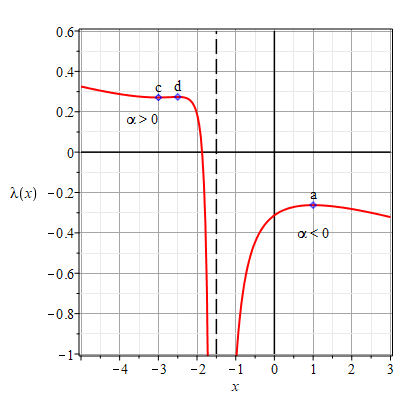
Figure 1: The functions $y=\lambda(x)$ for $\alpha>0$ (left) and $\alpha<0$ (right) and $m=5$.

(2) $m=4$. We have $x_{*}=-1$, $x_{c}=x_{d}=-2$, $\lambda_{c}=\lambda_{d}=1/4$ and $\lambda_{a}=-5/16=-0.3125$. Here $x_{c}=x_{d}=-2$ is the point of inflection. We obtain

$$n(\Lambda,\alpha)=\begin{cases}1,\ \Lambda\alpha>\lambda_{d},\\ 0,\ \Lambda\alpha=\lambda_{d},\\ 1,\ \Lambda\alpha<\lambda_{d}.\end{cases}$$ (3.44)

The functions $y=\lambda(x)$ for $m=4$ are depicted at Figure 2.

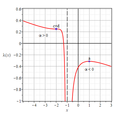
Figure 2: The functions $y=\lambda(x)$ for $\alpha>0$ (left) and $\alpha<0$ (right) and $m=4$.

(3) $m=3$. The functions $y=\lambda(x)$ for $m=3$ are depicted at Figure 3. We have $x_{*}=-1/2$, $x_{c}=-1$, $x_{d}=-3/2$, $\lambda_{c}=1/4$, $\lambda_{d}=15/64\approx 0.2344$ and $\lambda_{a}=-10/24$. In this subcase we have $\lambda_{d}<\lambda_{c}$ and hence

$$n(\Lambda,\alpha)=\begin{cases}1,\ \Lambda\alpha>\lambda_{c},\\ 2,\ \Lambda\alpha=\lambda_{c},\\ 3,\ \lambda_{d}<\Lambda\alpha<\lambda_{c},\\ 1,\ \Lambda\alpha\leq\lambda_{d}.\\ \end{cases}$$ (3.45)

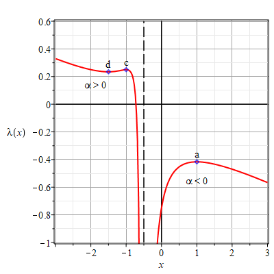
Figure 3: The functions $y=\lambda(x)$ for $\alpha>0$ (left) and $\alpha<0$ (right) and $m=3$.

Bounds on $\Lambda\alpha$ for $\alpha>0.$ If we summarize all cases presented above we get that for $\alpha>0$ exact solutions under consideration exist for all $\Lambda$

$$-\infty<\Lambda\alpha<+\infty,$$ (3.46)

when $m\neq 4$, while the extra restriction

$$\qquad\Lambda\alpha\neq\lambda_{d}.$$ (3.47)

should be imposed for $m=4$.

Let us consider the case $\alpha<0$. We have $\Lambda\alpha=\lambda(x)$, where $x>x_{*}$. Due to the relations (3.20), (3.27), (3.28) and (3.29) the function $\lambda(x)$ is monotonically increasing in the interval $(x_{*},x_{a}=1)$ from $-\infty$ to $\lambda_{a}$ and it is monotonically decreasing in the interval $(1,+\infty)$ from $\lambda_{a}$ to $-\infty$.

Here $x_{a}$ is a point of local maximum of the function $\lambda(x)$. This point is excluded from the solution.

The functions $y=\lambda(x)$ for $\alpha<0$ and $m=5,4,3$ are presented at Figures 1, 2, 3, respectively (at right panels: $x>x_{*}(m)$).

For the number of solutions (for $\alpha<0$) we obtain

$$n(\Lambda,\alpha)=\begin{cases}2,\ \Lambda(-\alpha)>|\lambda_{a}|,\\ 0,\ \Lambda(-\alpha)\leq|\lambda_{a}|.\\ \end{cases}$$ (3.48)

Here $x\neq x_{a}=1$. Hence, for $\alpha<0$ and big enough values of $\Lambda$ there exists two solutions $x_{1},x_{2}$: $x_{*}<x_{1}<x_{2}$.

Bounds on $\Lambda(-\alpha)$ for $\alpha<0.$ It follows from (3.48) that for $\alpha<0$ exact solutions under consideration exist if and only if

$$\Lambda(-\alpha)>|\lambda_{a}|=\frac{(D-2)(D-1)}{8(D-4)(D-3)},$$ (3.49)

see (3.38). This relation is valid for all $D=m+3>5$ ($m>2$).

4 Stability analysis

Here, we study the stability of exponential solutions (2.3). In what follows we use the results of refs. [25], when the total volume factor is non-static, i.e. if

$$S_{1}(v)=\sum_{i=1}^{n}v^{i}\neq 0.$$ (4.1)

As in [25], we impose the following restriction

$$({\rm R})\quad\det(L_{ij}(v))\neq 0$$ (4.2)

where

$$L=(L_{ij}(v))=(2G_{ij}-4\alpha G_{ijks}v^{k}v^{s}).$$ (4.3)

Here we remind that the cosmological ansatz with the (diagonal) metric

$$g=-dt\otimes dt+\sum_{i=1}^{n}e^{2\beta^{i}(t)}dy^{i}\otimes dy^{i},$$ (4.4)

gives us the set of equations [24, 25, 28]

$$E=G_{ij}h^{i}h^{j}+2\Lambda-\alpha G_{ijkl}h^{i}h^{j}h^{k}h^{l}=0,$$ (4.5)

$$Y_{i}=\frac{dL_{i}}{dt}+(\sum_{j=1}^{n}h^{j})L_{i}-\frac{2}{3}(G_{sj}h^{s}h^{j}-4\Lambda)=0$$ (4.6)

(for $\Lambda=0$ see [16, 17]), where $h^{i}=\dot{\beta}^{i}$, and

$$L_{i}=L_{i}(h)=2G_{ij}h^{j}-\frac{4}{3}\alpha G_{ijkl}h^{j}h^{k}h^{l},$$ (4.7)

$i=1,\ldots,n$.

It was proved in ref. [25] that a constant solution $(h^{i}(t))=(v^{i})$ ($i=1,\dots,n$; $n>3$) to eqs. (4.5), (4.6) obeying restrictions (4.1), (4.2) is stable under perturbations

$$h^{i}(t)=v^{i}+\delta h^{i}(t),$$ (4.8)

$i=1,\ldots,n$, as $t\to+\infty$ if

$$S_{1}(v)=\sum_{k=1}^{n}v^{k}>0$$ (4.9)

and it is unstable as $t\to+\infty$ if

$$S_{1}(v)=\sum_{k=1}^{n}v^{k}<0.$$ (4.10)

In our case $S_{1}(v)=mH+2h$, hence, due to $H>0$ the restriction (4.9) may be written as

$$x>-\frac{m}{2}=x_{d},$$ (4.11)

while the restriction (4.10) may be presented as

$$x<-\frac{m}{2}=x_{d}.$$ (4.12)

In the linear approximation the perturbations $\delta h^{i}$ obey the following set of linear equations [25]

$$C_{i}(v)\delta h^{i}=0,$$ (4.13)

$$L_{ij}(v)\delta\dot{h}^{j}=B_{ij}(v)\delta h^{j}.$$ (4.14)

Here

$$C_{i}(v)=2v_{i}-4\alpha G_{ijks}v^{j}v^{k}v^{s},$$ (4.15)

$$L_{ij}(v)=2G_{ij}-4\alpha G_{ijks}v^{k}v^{s},$$ (4.16)

$$B_{ij}(v)=-(\sum_{k=1}^{n}v^{k})L_{ij}(v)-L_{i}(v)+\frac{4}{3}v_{j},$$ (4.17)

where $v_{i}=G_{ij}v^{j}$, $L_{i}(v)=2v_{i}-\frac{4}{3}\alpha G_{ijks}v^{j}v^{k}v^{s}$ and $i,j,k,s=1,\dots,n$.

For the restrictions (4.1), (4.2) imposed, the set of equations (4.13), (4.14) has the following solution [25]

$$\delta h^{i}=A^{i}\exp(-S_{1}(v)t),$$ (4.18)

$$\sum_{i=1}^{n}C_{i}(v)A^{i}=0,$$ (4.19)

($A^{i}$ are constants) $i=1,\dots,n$.

For the vector $v$ from (3.1), obeying relations (3.3), the matrix $L$ has a block-diagonal form [25]

$$(L_{ij})={\rm diag}(L_{\mu\nu},L_{\alpha\beta}),$$ (4.20)

where

$$(L_{\mu\nu})=G_{\mu\nu}(2+4\alpha S_{HH}),$$ (4.21)

is $m\times m$ matrix and

$$L_{\alpha\beta}=G_{\alpha\beta}(2+4\alpha S_{hh}).$$ (4.22)

is $2\times 2$ matrix and

$$S_{HH}=(m-2)(m-3)H^{2}+4(m-2)Hh+2h^{2},$$ (4.23)

$$S_{hh}=m(m-1)H^{2}.$$ (4.24)

The matrix (4.20) is invertible only if

$$S_{HH}\neq-\frac{1}{2\alpha},$$ (4.25)

$$S_{hh}\neq-\frac{1}{2\alpha}.$$ (4.26)

We remind that the $k\times k$ matrix $(G_{ij})=(\delta_{ij}-1)$ is invertible for $k>1$. (Its inverse is $(G^{ij})=(\delta_{ij}-\frac{1}{k-1}$.)

Now, we prove that inequalities (4.25), (4.26) are obeyed if

$$x\neq-(m-2)=x_{c},$$ (4.27)

or $h\neq-(m-2)H$.

Let us suppose that (4.25) does not take place, i.e. $S_{HH}=-\frac{1}{2\alpha}$. Then using (3.5) we obtain

$$S_{HH}-Q=-2(H-h)((m-2)H+h)=0,$$ (4.28)

which implies due to $H-h\neq 0$ (see (3.3))

$$(m-2)H+h=0.$$ (4.29)

This relation contradicts to the restriction (4.27). The obtained contradiction proves the inequality (4.25).

Now let us suppose that (4.26) is not valid, i.e. $S_{hh}=-\frac{1}{2\alpha}$. Then using (3.5) we find

$$S_{hh}-Q=-2(h-H)(m-1)H=0.$$ (4.30)

But this relation contradicts $H>0$ and $H-h\neq 0$. This contradiction leads us to the proof of the inequality (4.26).

Thus, we have proved that relations (4.25) and (4.26) are valid and hence the restriction (4.2) is satisfied for our solutions.

Thus, we have proved the following proposition.

Proposition 2. The cosmological solutions under consideration, which obey $x=h/H\neq x_{i}$, $i=a,c,d$, where $x_{a}=1$, $x_{c}=-(m-2)$, $x_{d}=-\frac{m}{2}$, are stable if i) $x>x_{d}$ and unstable if ii) $x<x_{d}$.

Now we calculate the number of non-special stable solutions (i.e. obeying $x\neq x_{c}$) which are given by Proposition 2 (see item i)). We denote this number as $n_{*}(\Lambda,\alpha)$. By using the results from the previous section (e.g. illustrated by figures) we obtain for $\alpha>0$:

(1) $m>4$

$$n_{*}(\Lambda,\alpha)=\begin{cases}0,\ \Lambda\alpha\geq\lambda_{d},\\ 1,\ \Lambda\alpha<\lambda_{d};\\ \end{cases}$$ (4.31)

(2) $m=4$

$$n_{*}(\Lambda,\alpha)=\begin{cases}0,\ \Lambda\alpha\geq\lambda_{d}=\lambda_{c},\\ 1,\ \Lambda\alpha<\lambda_{d}=\lambda_{c};\\ \end{cases}$$ (4.32)

(3) $m=3$

$$n_{*}(\Lambda,\alpha)=\begin{cases}0,\ \Lambda\alpha\geq\lambda_{c},\\ 2,\ \lambda_{d}<\Lambda\alpha<\lambda_{c},\\ 1,\ \Lambda\alpha\leq\lambda_{d}.\\ \end{cases}$$ (4.33)

We see, that for $\alpha>0$ and small enough value of $\Lambda$ there exists at least one stable solution with $x\in(x_{d},x_{*})$.

Bounds on $\Lambda\alpha$ for stable solutions with $\alpha>0.$ Summarizing all cases presented above we find that for $\alpha>0$ stable exact solutions under consideration exist if and only if

$$\Lambda\alpha<\begin{cases}\ \lambda_{d}\ {\rm for}\ m\geq 4,\\ \ \lambda_{c}\ {\rm for}\ m=3,\end{cases}$$ (4.34)

where $\lambda_{c}=\lambda_{c}(m)$ and $\lambda_{d}=\lambda_{d}(m)$ are defined in (3.39) and (3.40), respectively.

In the case $\alpha<0$ we obtain

$$n_{*}(\Lambda,\alpha)=\begin{cases}2,\ \Lambda|\alpha|>|\lambda_{a}|,\\ 0,\ \Lambda|\alpha|\leq|\lambda_{a}|,\\ \end{cases}$$ (4.35)

i.e. $n_{*}(\Lambda,\alpha)=n(\Lambda,\alpha)$. Here the inequality $x\neq x_{a}=1$ was used. Thus, for $\alpha<0$ and big enough value of $\Lambda$ there exist two stable solution corresponding to $x=x_{1},x_{2}$ which obey $x_{*}<x_{1}<x_{2}$.

Bounds on $\Lambda|\alpha|$ for stable solutions with $\alpha<0.$ It follows from (4.35) that for $\alpha<0$ stable exact solutions under consideration exist if and only if the relation (3.49) is obeyed.

5 Solutions describing a small enough variation of $G$

Here we analyze the solutions by using the restriction on variation of the effective gravitational constant $G$, which is inversely proportional (in the Jordan frame) to the volume scale factor of the (anisotropic) internal space [21], i.e.

$$G={\rm const}\exp{[-(m-3)Ht-2ht]}.$$ (5.1)

By using (5.1) one can get the following formula for a dimensionless parameter of temporal variation of $G$ ($G$-dot):

$$\delta\equiv\frac{\dot{G}}{GH}=-(m-3+2x),\qquad x=h/H.$$ (5.2)

Here $H>0$ is the Hubble parameter.

Due to observational data, the variation of the gravitational constant is on the level of $10^{-13}$ per year and less.

For example, one can use, as it was done in ref. [21], the following bounds on the value of the dimensionless variation of the effective gravitational constant:

$$-0,65\cdot 10^{-3}<\delta<1,12\cdot 10^{-3}.$$ (5.3)

They come from the most stringent limitation on $G$-dot obtained by the set of ephemerides [41] and value of the Hubble parameter (at present) [38] when both are written with 95% confidence level [21].

When the value $\delta$ is fixed we get from (5.2)

$$x=x_{0}(\delta,m)\equiv-\frac{(m-3+\delta)}{2}.$$ (5.4)

We obtain

$$x_{0}(\delta,m)=-(m-3+\delta)/2>x_{*}(m)=-(m-2)/2$$ (5.5)

for $\delta<1$, e.g. when restrictions (5.3) are obeyed. In this case

$${\cal P}(x_{0}(\delta,m),m)=(m-1)(1-\delta)>0$$ (5.6)

and hence (see (3.9) )

$$\alpha<0.$$ (5.7)

Due to inequality (5.5) and relations $x_{c}(m)<x_{*}(m)$, $x_{d}(m)<x_{*}(m)$ all conditions in Proposition 2 are satisfied for $\delta<1$, e.g. when restrictions (5.3) are obeyed. This implies the stability of the solutions under consideration ($m>2$) with small enough variation of $G$, which obey the physical bounds (5.3).

We note that for $\delta=0$, i.e. for solutions with zero variation of $G$, we obtain from (3.12)

$$\Lambda|\alpha|=-\lambda(x_{0}(0,m))=\frac{2m^{2}-5m+9}{8(m-1)}>0,$$ (5.8)

$m>2$. For $m=3,4,5$ we find

$$\Lambda|\alpha|=\begin{cases}\ \frac{3}{4}\ {\rm for}\ m=3,\\ \ \frac{7}{8}\ {\rm for}\ m=4,\\ \ \frac{17}{16}\ {\rm for}\ m=5\end{cases}$$ (5.9)

with

$$x_{0}(0,m)=-(m-3)/2=\begin{cases}\ 0\ {\rm for}\ \ m=3,\\ \ -\frac{1}{2}\ {\rm for}\ m=4,\\ \ -1,\ {\rm for}\ m=5.\end{cases}$$ (5.10)

6 Conclusions

We have considered the $D$-dimensional Einstein-Gauss-Bonnet (EGB) model with the $\Lambda$-term. We have found a new class of cosmological solutions with diagonal metrics and exponential time dependence of two scale factors. The solutions are governed by two Hubble-like parameters $H>0$ and $h$, corresponding to flat subspaces of dimensions $m>2$ and $2$, respectively ($D=m+3$). Here the parameters $H$ and $h$ satisfy the following restrictions: $H\neq h$ and $mH+2h\neq 0$. The solutions obey the relation $(m-2)H+2h\neq 0$.

Any obtained solution may be considered as describing an exponential expansion of $3$-dimensional subspace (“our space”) with the Hubble parameter $H>0$ and anisotropic behaviour of $((m-3)+2)$-dimensional anisotropic internal space which expands in $(m-3)$ dimensions (with Hubble-like parameter $H$) and either contracts, or expands (with Hubble-like parameter $h$) or stable in $2$ dimensions. The solutions are governed by a polynomial equation of third order in $x=h/H$, which is readily solved in radicals for all values of $\Lambda$ and $\alpha$ in Appendix A. Here $\alpha=\alpha_{2}/\alpha_{1}$ where $\alpha_{1}$ and $\alpha_{2}$ are two non-zero constants of the model. The case $\Lambda=0$, which takes place only for $\alpha>0$, is outlined in Appendix B. We note that in our previous paper [1], devoted to $(1+m+l)$-dimensional solutions with $m>2$ and $l>2$, the polynomial master equation in $x=h/H$ was generically of fourth order. Here we have found the restrictions on $\Lambda$ which guarantee the existence of the solutions under consideration:

$$\Lambda\alpha\neq 1/4,\quad{\rm if}\ m=4$$ (6.1)

for $\alpha>0$ and

$$\Lambda|\alpha|>\frac{(D-2)(D-1)}{8(D-4)(D-3)}$$ (6.2)

for $\alpha<0$.

Using the scheme from ref. [25], we have proved that any of these solutions obeying the additional restriction $x\neq x_{c}=-(m-2)$, is stable (as $t\to+\infty$) if $x>x_{d}=-m/2$ and unstable if $x<x_{d}$.

We have also found that for $\alpha>0$ stable exact solutions exist if and only if:

$$\Lambda\alpha<\lambda_{d}$$ (6.3)

for $m\geq 4$ and

$$\Lambda\alpha<\lambda_{c},$$ (6.4)

for $m<4$, where $\lambda_{d}$ is defined in (3.40) and $\lambda_{c}$ is defined in (3.39). For $\alpha<0$ the all obtained exact solutions (obeying (6.2)) are stable.

We have shown that all (well-defined) solutions with small enough varation of the effective gravitational constant $G$ (in the Jordan frame) are stable.

The solutions presented here are different from those obtained in Ref. [1] for two non-coinciding Hubble-like parameters $H>0$ and $h$ corresponding to factor spaces of dimensions $m>2$ and $l>2$ with $mH+lh\neq 0$. In the case of Ref. [1] we have two branches with: (a) $\alpha>0$, $-\infty<\Lambda\alpha<\lambda_{+}(m,l)$ and (b) $\alpha<0$, $\Lambda|\alpha|>\lambda_{-}(m,l)$, where $\lambda_{\pm}(m,l)>0$. In the case $l=2$ and $\alpha>0$ the allowed values for $\Lambda$ are unbounded from the top and the bottom but they are bounded from the top when stable solutions are considered. For $l=2$, we have $x=h/H<x_{*}=-(m-2)/2$ for $\alpha>0$ and $x>x_{*}$ for $\alpha>0$, while in the case $l>2$ we get: $x_{-}<x<x_{+}<0$ for $\alpha>0$, and $x<x_{-}$ (unstable brunch) or $x>x_{+}$ (stable brunch) for $\alpha<0$.

Appendix

A The analytical solution to the master equation

For any $m>2$ the master equation (3.25) may be written as follows

$$x^{3}+bx^{2}+cx+d=0,\qquad$$ (A.1)

where

$$b=m-1+4\lambda(m-1),\qquad\qquad$$ (A.2)

$$c=(1/2)(m-1)m+4\lambda(m-1)(m-2),$$ (A.3)

$$d=(1/8)(m-2)m(m+1)+\lambda(m-1)(m-2)^{2}.$$ (A.4)

The standard (generically complex) Cardano solution to equation (A.1) gives us

$$x=x_{k}=-b/3+e_{k}\sqrt[3]{Z}-R/(e_{k}\sqrt[3]{Z}),$$ (A.5)

where

$$Z=(1/2)3^{-3/2}(\pm\sqrt{W})+Q,$$ (A.6)

$$W=27d^{2}+(4b^{2}-18c)bd+4c^{3}-b^{2}c^{2},$$ (A.7)

$$R=c/3-b^{2}/9,\qquad\qquad$$ (A.8)

$$Q=(bc-3d)/6-b^{3}/27,$$ (A.9)

and $e_{k}=\exp(2\pi ik/3)$ are cubic roots from unity, $k=0,1,2$. Here for a given value of square root $\sqrt{W}$ one should choose the sign $\pm$ such that $Z\neq 0$ and $\sqrt[3]{Z}$ is arbitrary (fixed) value of cubic root.

The calculations give us

$$W=((32q-m^{2}-2m)(8mq+m^{2}+3m+2)\times$$

$$\times(8(m-2)q-3m^{2}+13m-16))/64,$$ (A.10)

$$R=(-32q^{2}+8(m-4)q+(m+2)(m-1))/18,$$ (A.11)

$$Q=(-1024q^{3}+384(m-4)q^{2}+24(m^{2}+10m-20)q$$

$$-(m+2)(7m^{2}-17m-8))/432,$$ (A.12)

where $q=\lambda(m-1)=\Lambda\alpha(m-1)$.

Here $W=-\Delta$, where $\Delta$ is discriminant corresponding to (A.1). We get

$$W=32(m-1)^{3}m(m-2)(\lambda-\lambda_{a})(\lambda-\lambda_{c})(\lambda-\lambda_{d}),$$ (A.13)

where $\lambda_{a},\lambda_{c},\lambda_{d}$ are defined in (3.38), (3.39), (3.40), respectively.

It is known that for $\Delta>0$ the equation (A.1) has three different real solutions, while for $\Delta<0$ it has is only one real solutions. For $\Delta=0$ we have: either i) two different real solutions (two roots are coinciding) or ii) or one real solutions (all three roots are coinciding). One can readily verify that these facts confirm the classifiction of the number of solutions presented in Section 3 (up to exclusion one of the solutions for $\lambda=\lambda_{d}$ corresponding to $x=x_{d}$.) We note that the case $\Delta=0$ takes place when $\lambda=\lambda_{i}$ for some $i=a,c,d$. In the subcase ii) we obtain solutions: $x=x_{a}=1$ (for $\alpha<0$, $\lambda=\lambda_{a}$) and $x=x_{d}=x_{c}=-2$ (for $\alpha>0$, $m=4$ and $\lambda=\lambda_{c}=\lambda_{d}=1/4$), which are forbidden by our restrictions.

B The case $\Lambda=0$

For $\Lambda\alpha=\lambda=0$ we obtain

$$W=m(m+1)(m+2)^{2}(3m^{2}-13m+16)/64=$$

$$32(m-1)^{3}m(m-2)(-\lambda_{a})\lambda_{c}\lambda_{d}>0$$ (B.14)

for $m>2$ or $\Delta<0$. Hence in this case we have only one real solution to master equation which is agreement with our graphical analysis from Section 3. This solution takes place only for $\alpha>0$. It is given by the relations (following from those presented above)

$$x=\sqrt[3]{Z}-R/\sqrt[3]{Z}-(m-1)/3,\qquad$$ (B.15)

$$R=(m-1)(m+2)/18,\qquad\qquad\qquad$$ (B.16)

$$Z=2^{-4}3^{-3/2}(m+2)\sqrt{m(m+1)(3m^{2}-13m+16)}+Q,$$ (B.17)

$$Q=-((m+2)(7m^{2}-17m-8))/432,\qquad$$ (B.18)

$m>2$. It may be shown that $Z>0$ for all natural $m$. The calculations give us the following approximate values:

$$x\approx\begin{cases}-0.72212,\ {\rm for}\ m=3,\\ -1.32219\ {\rm for}\ m=4,\\ -1.86971\ {\rm for}\ m=5.\end{cases}$$ (B.19)

Acknowledgments

This paper has been supported by the RUDN University Strategic Academic Leadership Program (recipient V.D.I., mathematical model development). The reported study was funded by RFBR, project number 19-02-00346 (recipient A.A.K., simulation model development).

References

- [1] V.D. Ivashchuk and A.A. Kobtsev, Stable exponential cosmological solutions with two factor spaces in the Einstein-Gauss-Bonnet model with a -term, Gen. Relativ. Gravit., 50, 119, 1-30 (2018).
- [2] V.D. Ivashchuk, On Stability of Exponential Cosmological Type Solutions with Two Factor Spaces in the Einstein-Gauss-Bonnet Model with a -term, Grav. Cosmol., Vol. 26, No. 1, 16-21 (2020).
- [3] B. Zwiebach, Curvature squared terms and string theories, Phys. Lett. B 156, 315 (1985).
- [4] E.S. Fradkin and A.A. Tseytlin, Effective action approach to superstring theory, Phys. Lett. B 160, 69-76 (1985).
- [5] D. Gross and E. Witten, Superstrings modifications of Einstein’s equations, Nucl. Phys. B 277, 1 (1986).
- [6] D. Lovelock, The Einstein tensor and its generalizations, J. Math. Phys. 12, 498 (1971); doi:10.1063/1.1665613.
- [7] D. Lovelock, The four-dimensionality of space and the Einstein tensor, J. Math. Phys. 13, 874 (1972); doi: 10.1063/1.1666069.
- [8] H. Ishihara, Cosmological solutions of the extended Einstein gravity with the Gauss-Bonnet term, Phys. Lett. B 179, 217 (1986).
- [9] N. Deruelle, On the approach to the cosmological singularity in quadratic theories of gravity: the Kasner regimes, Nucl. Phys. B 327, 253-266 (1989).
- [10] S. Nojiri and S.D. Odintsov, Introduction to modified gravity and gravitational alternative for Dark Energy, Int. J. Geom. Meth. Mod. Phys. 4, 115-146 (2007); hep-th/0601213.
- [11] E. Elizalde, A.N. Makarenko, V.V. Obukhov, K.E. Osetrin and A.E. Filippov, Stationary vs. singular points in an accelerating FRW cosmology derived from six-dimensional Einstein-Gauss-Bonnet gravity, Phys. Lett. B 644, 1-6 (2007); hep-th/0611213.
- [12] K. Bamba, Z.-K. Guo and N. Ohta, Accelerating Cosmologies in the Einstein-Gauss-Bonnet theory with dilaton, Prog. Theor. Phys. 118, 879-892 (2007); arXiv: 0707.4334.
- [13] I.V. Kirnos and A.N. Makarenko, Accelerating cosmologies in Lovelock gravity with dilaton, Open Astron. J. 3, 37-48 (2010); arXiv: 0903.0083.
- [14] S.A. Pavluchenko, On the general features of Bianchi-I cosmological models in Lovelock gravity, Phys. Rev. D 80, 107501 (2009); arXiv: 0906.0141.
- [15] I.V. Kirnos, A.N. Makarenko, S.A. Pavluchenko and A.V. Toporensky, The nature of singularity in multidimensional anisotropic Gauss-Bonnet cosmology with a perfect fluid, Gen. Relativ. Gravit. 42, 2633-2641 (2010); arXiv: 0906.0140.
- [16] V.D. Ivashchuk, On anisotropic Gauss-Bonnet cosmologies in (n + 1) dimensions, governed by an n-dimensional Finslerian 4-metric, Grav. Cosmol. 16(2), 118-125 (2010); arXiv: 0909.5462.
- [17] V.D. Ivashchuk, On cosmological-type solutions in multidimensional model with Gauss-Bonnet term, Int. J. Geom. Meth. Mod. Phys. 7(5), 797-819 (2010); arXiv: 0910.3426.
- [18] K.-i. Maeda and N. Ohta, Cosmic acceleration with a negative cosmological constant in higher dimensions, JHEP 1406: 095 (2014); arXiv:1404.0561.
- [19] D. Chirkov, S. Pavluchenko and A. Toporensky, Exact exponential solutions in Einstein-Gauss-Bonnet flat anisotropic cosmology, Mod. Phys. Lett. A 29, 1450093 (11 pages) (2014); arXiv:1401.2962.
- [20] D. Chirkov, S.A. Pavluchenko and A. Toporensky, Non-constant volume exponential solutions in higher-dimensional Lovelock cosmologies, Gen. Relativ. Gravit. 47: 137 (33 pages) (2015); arXiv: 1501.04360.
- [21] V.D. Ivashchuk and A.A. Kobtsev, On exponential cosmological type solutions in the model with Gauss-Bonnet term and variation of gravitational constant, Eur. Phys. J. C 75: 177 (12 pages) (2015); Erratum, Eur. Phys. J. C (2016) 76: 584; arXiv:1503.00860.
- [22] S.A. Pavluchenko, Stability analysis of exponential solutions in Lovelock cosmologies, Phys. Rev. D 92, 104017 (2015); arXiv: 1507.01871.
- [23] S.A. Pavluchenko, Cosmological dynamics of spatially flat Einstein-Gauss-Bonnet models in various dimensions: Low-dimensional -term case, Phys. Rev. D 94, 084019 (2016); arXiv: 1607.07347.
- [24] K.K. Ernazarov, V.D. Ivashchuk and A.A. Kobtsev, On exponential solutions in the Einstein-Gauss-Bonnet cosmology, stability and variation of G, Grav. Cosmol., 22 (3), 245-250 (2016).
- [25] V.D. Ivashchuk, On stability of exponential cosmological solutions with non-static volume factor in the Einstein-Gauss-Bonnet model, Eur. Phys. J. C 76 431 (2016) (10 pages); arXiv: 1607.01244v2.
- [26] K.K. Ernazarov and V.D. Ivashchuk, Stable exponential cosmological solutions with zero variation of G in the Einstein-Gauss-Bonnet model with a -term, Eur. Phys. J. C 77: 89 (2017) (6 pages); arXiv:1612.08451.
- [27] S. Pabluchenko, Realistic Compactification Models in Einstein-Gauss-Bonnet Gravity, Particles, 1 (1), 4 (21 pages) (2018); arXiv: 1803.01887.
- [28] V. D. Ivashchuk and A. A. Kobtsev, Exact exponential cosmological solutions with two factor spaces of dimension in EGB model with a -term, Int. J. Geom. Meth. Mod. Phys., 16 (2), 1950025 (26 pages) (2019).
- [29] A.G. Riess et al. Observational evidence from supernovae for an accelerating universe and a cosmological constant, Astron. J. 116, 1009-1038 (1998).
- [30] S. Perlmutter et al., Measurements of Omega and Lambda from 42 High-Redshift Supernovae, Astrophys. J. 517, 565-586 (1999).
- [31] M. Kowalski, D. Rubin et al., Improved cosmological constraints from new, old and combined supernova datasets, Astrophys. J. 686 (2), 749-778 (2008); arXiv: 0804.4142.
- [32] D.G. Boulware and S. Deser, String generated gravity models, Phys. Rev. Lett. 55, 2656 (1985).
- [33] J.T. Wheeler, Symmetric solutions to the Gauss-Bonnet extended Einstein equations, Nucl. Phys. B 268, 737 (1986).
- [34] J.T. Wheeler, Symmetric solutions to the maximally Gauss-Bonnet extended Einstein equations, Nucl. Phys. B 273, 732 (1986).
- [35] D.L. Wiltshire, Spherically symmetric solutions of Einstein-Maxwell theory with a Gauss-Bonnet term, Phys. Lett. B 169, 36 (1986).
- [36] R.-G. Cai, Gauss-Bonnet black holes in AdS spaces, Phys. Rev. D 65, 084014 (2002); hep-th/0109133.
- [37] C. Garraffo and G. Giribet, The Lovelock Black Holes, Mod. Phys. Lett. A 23: 1801-1818 (2008); arXiv: 0805.3575v4 [gr-qc].
- [38] P.A.R. Ade et al. [Planck Collaboration], Planck 2013 results. I. Overview of products and scientific results, Astron. Astrophys. 571, A1 (2014); arXiv: 1303.5076.
- [39] M. Rainer and A. Zhuk, Einstein and Brans-Dicke frames in multidimensional cosmology, Gen. Relativ. Gravit. 32, 79-104 (2000); gr-qc/9808073.
- [40] V.D. Ivashchuk and V.N. Melnikov, Multidimensional Gravity with Einstein Internal Spaces, Grav. Cosmol. 2 (3), 211-220 (1996); hep-th/9612054.
- [41] E.V. Pitjeva, Updated IAA RAS Planetary Ephemerides-EPM2011 and Their Use in Scientific Research, Astron. Vestnik 47 (5), 419-435 (2013); arXiv: 1308.6416.