SSMBA: Self-Supervised Manifold Based Data Augmentation for Improving Out-of-Domain Robustness

Abstract

Models that perform well on a training domain often fail to generalize to out-of-domain (OOD) examples. Data augmentation is a common method used to prevent overfitting and improve OOD generalization. However, in natural language, it is difficult to generate new examples that stay on the underlying data manifold. We introduce SSMBA, a data augmentation method for generating synthetic training examples by using a pair of corruption and reconstruction functions to move randomly on a data manifold. We investigate the use of SSMBA in the natural language domain, leveraging the manifold assumption to reconstruct corrupted text with masked language models. In experiments on robustness benchmarks across 3 tasks and 9 datasets, SSMBA consistently outperforms existing data augmentation methods and baseline models on both in-domain and OOD data, achieving gains of 0.8% accuracy on OOD Amazon reviews, 1.8% accuracy on OOD MNLI, and 1.4 BLEU on in-domain IWSLT14 German-English.

1 Introduction

Training distributions often do not cover all of the test distributions we would like a supervised classifier or model to perform well on. Often, this is caused by biased dataset collection (Torralba and Efros, 2011) or test distribution drift over time (Quionero-Candela et al., 2009). Therefore, a key challenge in training machine learning models in these settings is ensuring they are robust to unseen examples. Since it is impossible to generalize to the entire distribution, methods often focus on the adjacent goal of out-of-domain robustness.

Data augmentation is a common technique used to improve out-of-domain (OOD) robustness by synthetically generating new training examples (Simard et al., 1998), often by perturbing existing examples in the input space (Perez and Wang, 2017). If data concentrates on a low-dimensional manifold (Chapelle et al., 2006), then these synthetic examples should lie in a manifold neighborhood of the original examples (Chapelle et al., 2000). Training models to be robust to such local perturbations has been shown to be effective in improving performance and generalization in semi-supervised and self-supervised settings (Bachman et al., 2014; Szegedy et al., 2014; Sajjadi et al., 2016). When the underlying data manifold exhibits easy-to-characterize properties, as in natural images, simple transformations such as translation and rotation can quickly generate local training examples. However, in domains such as natural language, it is much more difficult to find a set of invariances that preserves meaning or semantics.

Figure 1: SSMBA moves along the data manifold $\mathcal{M}$ by using a corruption function to perturb an example $x$ off the data manifold, then using a reconstruction function to project it back on.

In this paper we propose Self-Supervised Manifold Based Data Augmentation (SSMBA): a data augmentation method for generating synthetic examples in domains where the data manifold is difficult to heuristically characterize. Motivated by the use of denoising auto-encoders as generative models (Bengio et al., 2013), we use a corruption function to stochastically perturb examples off the data manifold, then use a reconstruction function to project them back on (Figure 1). This ensures new examples lie within the manifold neighborhood of the original example. SSMBA is applicable to any supervised task, requires no task-specific knowledge, and does not rely on class- or dataset-specific fine-tuning.

We investigate the use of SSMBA in the natural language domain on 3 diverse tasks spanning both classification and sequence modelling: sentiment analysis, natural language inference, and machine translation. In experiments across 9 datasets and 4 model types, we show SSMBA consistently outperforms baseline models and other data augmentation methods on both in-domain and OOD data.

2 Background and Related Work

2.1 Data Augmentation in NLP

The problem of domain adaptation and OOD robustness is well established in NLP (Blitzer et al., 2007; Daumé III, 2007; Hendrycks et al., 2020). Existing work on improving generalization has focused on data augmentation, where synthetically generated training examples are used to augment an existing dataset. It is hypothesized that these examples induce robustness to local perturbations, which has been shown to be effective in semi-supervised and self-supervised settings (Bachman et al., 2014; Szegedy et al., 2014; Sajjadi et al., 2016).

Existing task-specific methods (Kafle et al., 2017) and word-level methods (Zhang et al., 2015; Xie et al., 2017; Wei and Zou, 2019) are based on human-designed heuristics. Back-translation from or through another language has been applied in the context of machine translation (Rico Sennrich, 2016), question answering (Yu et al., 2018), and consistency training (Xie et al., 2019). More recent work has used word embeddings (Wang and Yang, 2015) and LSTM language models (Fadaee et al., 2017) to perform word replacement. Other methods focus on fine-tuning contextual language models (Kobayashi, 2018; Wu et al., 2019b; Kumar et al., 2020) or large generative models (Anaby-Tavor et al., 2020; Yang et al., 2020; Kumar et al., 2020) to generate synthetic examples.

2.2 VRM and the Manifold Assumption

Vicinal Risk Minimization (VRM) (Chapelle et al., 2000) formalizes data augmentation as enlarging the training set support by drawing samples from a vicinity of existing training examples. Typically the vicinity of a training example is defined using dataset-dependent heuristics. For example, in computer vision, examples are generated using scale augmentation (Simonyan and Zisserman, 2015), color augmentation (Krizhevsky et al., 2012), and translation and rotation (Simard et al., 1998).

The manifold assumption states that high dimensional data concentrates around a low-dimensional manifold (Chapelle et al., 2006). This assumption allows us to define the vicinity of a training example as its manifold neighborhood, the portion of the neighborhood that lies on the data manifold. Recent methods have used the manifold assumption to improve robustness by moving examples towards a decision boundary (Kanbak et al., 2018), generating adversarial examples Szegedy et al. (2014); Miyato et al. (2017), interpolating between pairs of examples (Zhang et al., 2018), or finding affine transforms (Paschali et al., 2019).

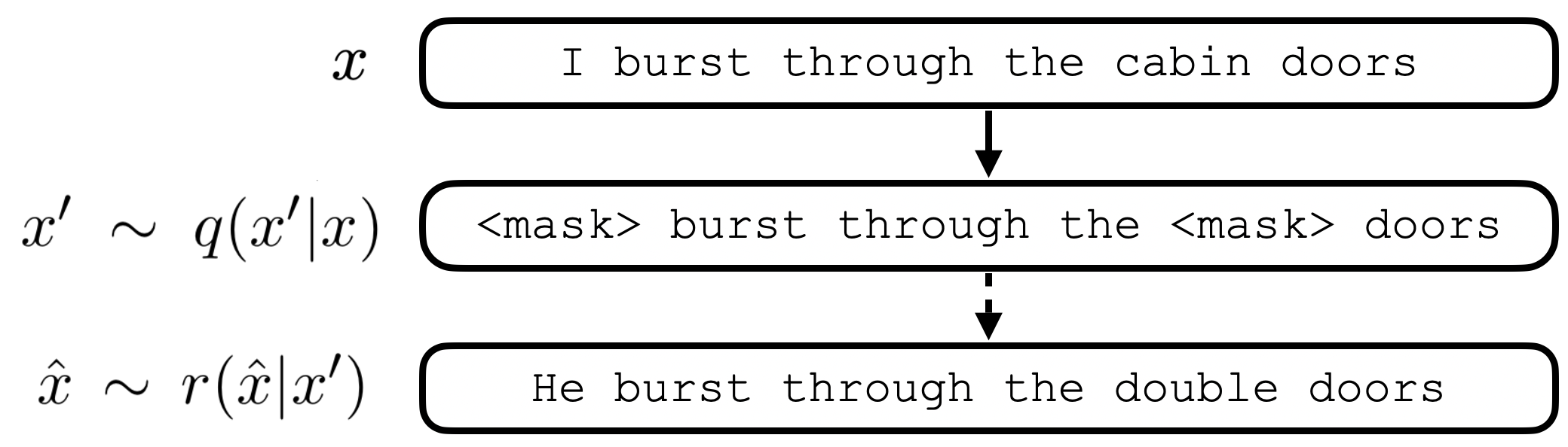
Figure 2: To sample from an MLM DAE, we apply the MLM corruption $q$ to the original sentence then reconstruct the corrupted sentence using our DAE $r$.

2.3 Sampling from Denoising Autoencoders

A denoising autoencoder (DAE) is an autoencoder trained to reconstruct a clean input $x$ from a stochastically corrupted one $x^{\prime}\sim q(x^{\prime}|x)$ by learning a conditional distribution $P_{\theta}(x|x^{\prime})$ (Vincent et al., 2008). We can sample from a DAE by successively corrupting and reconstructing an input using the following pseudo-Gibbs Markov chain: $x_{t}^{\prime}\sim q(x^{\prime}|x_{t-1})$, $x_{t}\sim P_{\theta}(x|x^{\prime}_{t}).$ As the number of training examples increases, the asymptotic distribution $\pi_{n}(x)$ of the generated samples approximate the true data-generating distribution $P(x)$ (Bengio et al., 2013). This corruption-reconstruction process allows for sampling directly along the manifold that $P(x)$ concentrates on.

2.4 Masked Language Models

Recent advances in unsupervised representation learning for natural language have relied on pre-training models on a masked language modeling (MLM) objective (Devlin et al., 2018; Liu et al., 2019). In the MLM objective, a percentage of the input tokens are randomly corrupted and the model is asked to reconstruct the original token given its left and right context in the corrupted sentence. We use MLMs as DAEs (Lewis et al., 2019) to sample from the underlying natural language distribution by corrupting and reconstructing inputs (Figure 2).

3 SSMBA: Self-Supervised Manifold Based Augmentation

1:Require: perturbation function $q$ reconstruction function $r$

2:Input: Dataset $\mathcal{D}=\{(x_{1},y_{1})\ldots(x_{n},y_{n})\}$ number of augmented examples $m$

3:function SSMBA($\mathcal{D}$, $m$)

4:    train a model $f$ on $\mathcal{D}$

5:    for $(x_{i},y_{i})\in\mathcal{D}$ do

6:        for $j\in 1\ldots m$ do

7:            sample perturbed $x_{ij}^{\prime}\sim q(x^{\prime}|x_{i})$

8:            sample reconstructed $\hat{x}_{ij}\sim r(\hat{x}|x_{ij}^{\prime})$

9:            generate $\hat{y}_{ij}\leftarrow f(\hat{x}_{ij})$ or preserve

10:            the original $y_{i}$

11:        end for

12:    end for

13:    let $\mathcal{D}^{aug}=\{(\hat{x}_{ij},\hat{y}_{ij})\}_{i=1\ldots n,j=1\ldots m}$

14:    augment $\mathcal{D}^{\prime}\leftarrow\mathcal{D}\cup\mathcal{D}^{aug}$

15:    return $\mathcal{D}^{\prime}$

16:end function

Algorithm 1 SSMBA

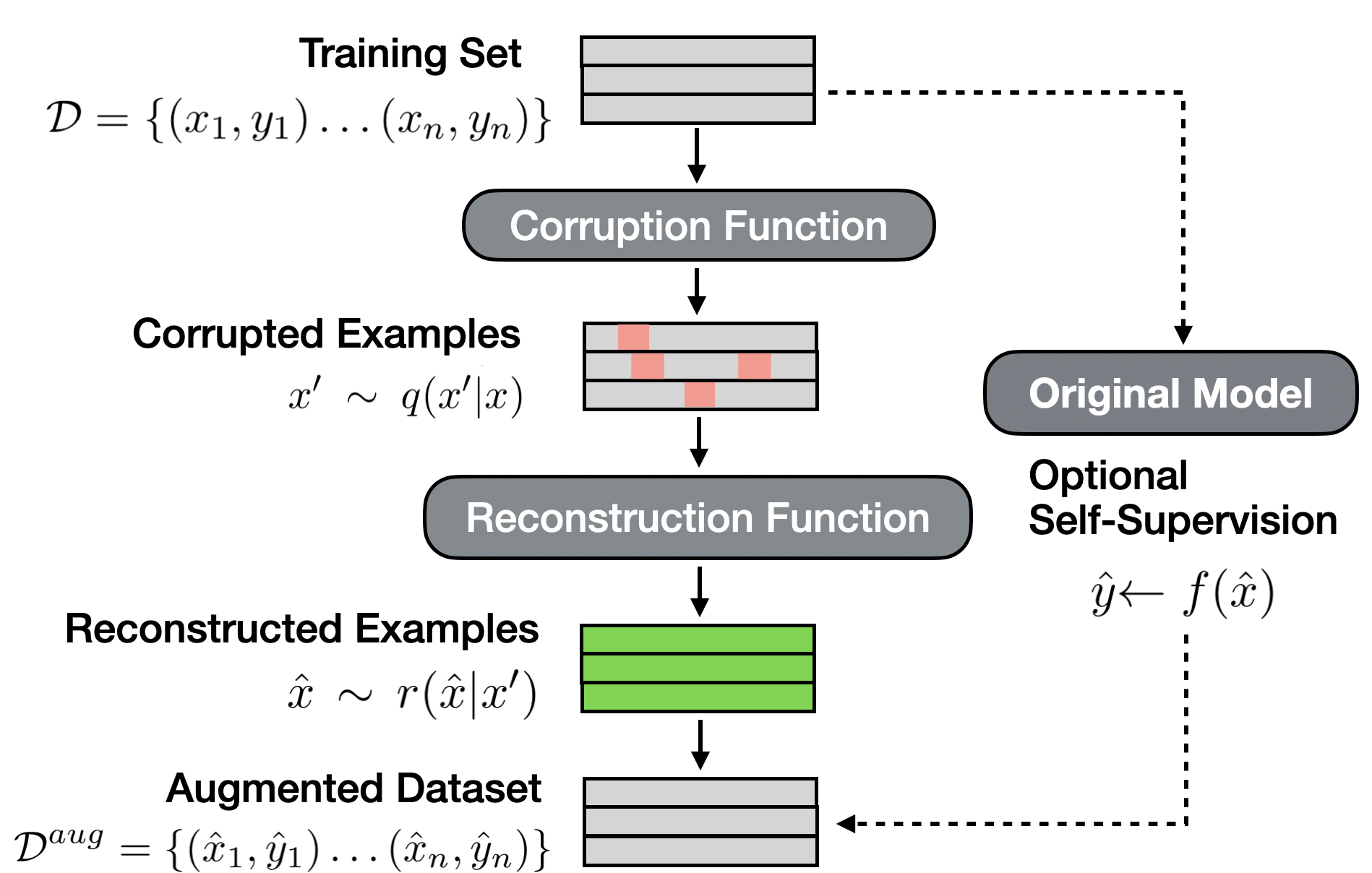
Figure 3: SSMBA generates synthetic examples by corrupting then reconstructing the original training inputs. To form the augmented dataset, corresponding outputs are preserved from the original data or generated from a supervised model $f$ trained on the original data.

We now describe Self-Supervised Manifold Based Data Augmentation. Let our original dataset $\mathcal{D}$ consist of pairs of input and output vectors $\mathcal{D}=\{(x_{1},y_{1})\ldots(x_{n},y_{n})\}$. We assume the input points concentrate around an underlying lower dimensional data manifold $\mathcal{M}$. Let $q$ be a corruption function from which we can draw a sample $x^{\prime}\sim q(x^{\prime}|x)$ such that $x^{\prime}$ no longer lies on $\mathcal{M}$. Let $r$ be a reconstruction function from which we can draw a sample $\hat{x}\sim r(\hat{x}|x^{\prime})$ such that $\hat{x}$ lies on $\mathcal{M}$.

To generate an augmented dataset, we take each pair $(x_{i},y_{i})\in\mathcal{D}$ and sample a perturbed $x_{i}^{\prime}\sim q(x^{\prime}|x_{i})$. We then sample a reconstructed $\hat{x}_{ij}\sim r(\hat{x}|x_{i}^{\prime})$. A corresponding vector $\hat{y}_{ij}$ can be generated by preserving $y_{i}$, or, since examples in the manifold neighborhood may cross decision boundaries on more sensitive tasks, by using a teacher model trained on the original data. This operation can be repeated to generate multiple augmented examples for each input example. These new examples form a dataset that we can augment the original training set with. We can then train an augmented model on the new augmented dataset.

In this paper we investigate SSMBA’s use on natural language tasks, using the MLM training corruption function as our corruption function $q$ and a pre-trained BERT model as our reconstruction model $r$. Different from other data augmentation methods, SSMBA does not rely on task-specific knowledge, requires no dataset-specific fine-tuning, and is applicable to any supervised natural language task. SSMBA requires only a pair of functions $q$ and $r$ used to generate data.

4 Datasets

To empirically evaluate our proposed algorithm, we select 9 datasets – 4 sentiment analysis datasets, 2 natural language inference (NLI) datasets, and 3 machine translation (MT) datasets. Table 1 and Appendix A provide dataset summary statistics. All datasets either contain metadata that can be used to split the samples into separate domains or similar datasets that are treated as separate domains.

4.1 Sentiment Analysis

The Amazon Review Dataset (Ni et al., 2019) contains product reviews from Amazon. Following Hendrycks et al. 2020, we form two datasets: AR-Full contains reviews from the 10 largest categories, and AR-Clothing contains reviews in the clothing category separated into subcategories by metadata. Since the reviews in AR-Clothing come from the same top-level category, the amount of domain shift is much less than that of AR-Full. Models predict a review’s 1 to 5 star rating.

SST2 (Socher et al., 2013) contains movie review excerpts. Following Hendrycks et al. 2020 we pair this dataset with the IMDb dataset (Maas et al., 2011), which contains full length movie reviews. We call this pair the Movies dataset. Models predict a movie review’s binary sentiment.

The Yelp Review Dataset contains restaurant reviews with associated business metadata which we preprocess following Hendrycks et al. 2020. Models predict a review’s 1 to 5 star rating.

Dataset	Domain	$n$	$l$	Train	Test
AR-Clothing	*	4	35	25k†	2k
AR-Full	*	10	67	25k†	2k
Yelp	*	4	138	25k†	2k
Movies	SST2	-	11	66k	1k
	IMDb	-	296	46k	2k
MNLI	*	10	36	80k	1k
ANLI	R1	-	92	17k	1k
	R2	-	90	46k	1k
	R3	-	82	100k	1k
IWSLT	-	1	24	160k	7k
OPUS	Medical	5	15	1.1m	2k
de-rm	Law	-	22	100k	2k
	Blogs	-	25	-	2k

Table 1: Dataset summary statistics. $n$: number of domains. $l$: average tokenized input length. A * in the domain column indicates that the statistics are identical across domains within that dataset. Training sets marked with a $\dagger$ are sampled randomly from a larger dataset. Refer to Appendix A for more information.

4.2 Natural Language Inference

MNLI (Williams et al., 2018) is a corpus of NLI data from 10 distinct genres of written and spoken English. We train on the 5 genres with training data and test on all 10 genres. Since the dataset does not include labeled test data, we use the validation set as our test set and sample 2000 examples from each training set for validation.

ANLI (Nie et al., 2019) is a corpus of NLI data designed adversarially by humans such that state-of-the-art models fail to classify examples correctly. The dataset consists of three different levels of difficulty which we treat as separate textual domains.

4.3 Machine Translation

Following Müller et al. 2019, we consider two translation directions, German$\to$English (de$\to$en) and German$\to$Romansh (de$\to$rm). Romansh is a low-resource language with an estimated 40,000 native speakers where OOD robustness is of practical relevance (Müller et al., 2019).

In the de$\to$en direction, we use IWSLT14 de$\to$en (Cettolo et al., 2014) as a widely-used benchmark to test in-domain performance. We also use the OPUS (Tiedemann, 2012) dataset to test OOD generalization. We train on highly specific in-domain data (medical texts) and disparate out-of-domain data (Koran text, Ubuntu localization files, movie subtitles, and legal text). Since domains share very little similarities in language, generalization to out-of-domain text is extremely difficult. In the de$\to$rm direction, we use a training set consisting of the Allegra corpus (Scherrer and Cartoni, 2012) and Swiss press releases. We use blog posts from Convivenza as a test domain.

5 Experimental Setup

5.1 Model Types

For sentiment analysis tasks, we investigate LSTMs (Hochreiter and Schmidhuber, 1997) and convolutional neural networks (CNNs). For NLI tasks, we investigate fine-tuned RoBERTa_BASE models (Liu et al., 2019), which are pretrained bidirectional transformers (Vaswani et al., 2017). On both tasks, representations from the encoder are fed into an feed-forward neural network for classification. For MT tasks, we train transformers (Vaswani et al., 2017). For all models, word embeddings are initialized randomly and trained end-to-end with the model. We do not initialize with pre-trained word embeddings to maintain consistency across all models and tasks. Model hyperparameters are tuned to maximize performance on in-domain validation data. Training details and hyperparameters for all models are provided in Appendix C.

5.2 SSMBA Settings

For all experiments we use the MLM corruption function as our corruption function $q$. We tune tune the total percentage of tokens corrupted, leaving the percentages of specific corruption operations (80% masked, 10% random, 10% unmasked) the same. For sentiment analysis and NLI experiments we use a pre-trained RoBERTa_BASE model as our reconstruction function $r$, and for translation experiments we use a pre-trained German BERT model (Chan et al., 2020). For each input example, we generate 5 augmented examples using unrestricted sampling. For translation experiments, target side translations are generated with beam search with width 5. SSMBA hyperparameters, including augmented example labelling method and corruption percentage, are chosen based on in-domain validation performance. Hyperparameters for each dataset are provided in Appendix D.

		AR-Full		AR-Clothing		Movies		Yelp		Average
Model	Augmentation	ID	OOD	ID	OOD	ID	OOD	ID	OOD	ID	OOD
RNN	None	69.46	66.32	69.25	67.80	90.74	71.94	62.51	61.28	70.16	66.17
	EDA	67.32	64.47	66.87	65.21	88.43	68.3	58.39	57.19	67.56	63.55
	CBERT	69.94	66.77	69.56	68.10	91.01	72.11	63.17	61.75	70.17	66.57
	UDA	69.92	66.97	69.98	68.24	90.05	69.73	63.40	62.13	70.64	66.53
	SSMBA	70.38∗†	67.41∗†	70.19	68.60∗†	89.61	73.20	63.85	62.83∗†	70.96	67.31
CNN	None	70.67	67.64	70.14	68.52	92.92	72.11	65.13	64.46	71.68	67.63
	EDA	68.52	66.03	67.76	66.17	91.22	74.20	60.99	59.88	69.13	65.65
	CBERT	70.62	67.70	70.13	68.23	92.92	71.56	65.09	64.19	71.65	67.49
	UDA	70.80	68.06	70.29	68.70	92.63	72.55	65.22	64.32	71.77	67.89
	SSMBA	71.10∗	68.18∗	70.74	69.04∗	92.93	74.67	65.59	64.81∗†	72.11	68.33

Table 2: Average in-domain (ID) and out-of-domain (OOD) accuracy (%) for models trained on sentiment analysis datasets. Average performance across datasets is weighted by number of domains contained in each dataset. Accuracies marked with a $*$ and $\dagger$ are statistically significantly higher than unaugmented models and the next best model respectively, both with $p<0.01$.

5.3 Baselines

On sentiment analysis and NLI tasks, we compare against 3 data augmentation methods. Easy Data Augmentation (EDA) (Wei and Zou, 2019) is a heuristic method that randomly replaces synonyms and inserts, swaps, and deletes words. Conditional Bert Contextual Augmentation (CBERT) (Wu et al., 2019b) finetunes a class-conditional BERT model and uses it to generate sentences in a process similar to our own. Unsupervised Data Augmentation (UDA) (Xie et al., 2020) translates data to and from a pivot language to generate paraphrases. We adapt UDA for supervised classification tasks by training directly on the backtranslated data.

On translation tasks, we compare only against methods which do not require additional target side monolingual data. Word dropout (Sennrich et al., 2016) randomly chooses words in the source sentence to set to zero embeddings. Reward Augmented Maximum Likelihood (RAML) (Norouzi et al., 2016) samples noisy target sentences based on an exponential of their Hamming distance from the original sentence. SwitchOut (Wang et al., 2018) applies a noise function similar to RAML to both the source and target side. We use publicly available implementations for all methods.

5.4 Evaluation Method

We train LSTM and CNN models with 10 random seeds, RoBERTa models with 5 random seeds, and transformer models with 3 random seeds. Models are trained separately on each domain then evaluated on all domains, and performance is averaged across seeds and test domains. We report the average in-domain (ID) and OOD performance across all train domains. On sentiment analysis and NLI tasks we report accuracy, and on translation we report uncased tokenized BLEU (Papineni et al., 2002) for IWSLT and cased, detokenized BLEU with SacreBLEU (Post, 2018) for all others. Statistical testing details are in Appendix E.

6 Results

6.1 Sentiment Analysis

Table 2 present results on sentiment analysis. Across all datasets, models trained with SSMBA outperform baseline models and all other data augmentation methods on OOD data. On ID data, SSMBA outperforms baseline models and other data augmentation methods on all datasets for CNN models, and 3/4 datasets for RNN models. On average, SSMBA improves OOD performance by 1.1% for RNN models and 0.7% for CNN models, and ID performance by 0.8% for RNN models and 0.4% for CNN model. Other methods achieve much smaller OOD generalization gains and perform worse than baseline models on multiple datasets.

On the AR-Full dataset, RNNs trained with SSMBA demonstrate improvements in OOD accuracy of 1.1% over baseline models. On the AR-Clothing dataset, which exhibits less domain shift than AR-Full, RNNs trained with SSMBA exhibit slightly lower OOD improvement. CNN models exhibit about the same boost in OOD accuracy across both Amazon review datasets.

On the Movies dataset where we observe a large difference in average sentence length between the two domains, SSMBA still manages to present considerable gains in OOD performance. Although RNNs trained with SSMBA fail to improve ID performance, their OOD performance in this setting still beats other data augmentation methods.

On the Yelp dataset, we observe large performance gains on both ID and OOD data for RNN models. The improvements on CNN models are more modest, but notably our method is the only one that improves OOD generalization.

	MNLI		ANLI
Augmentation	ID	OOD	ID	OOD
None	84.29	80.61	42.54	43.80
EDA	83.44	80.34	45.59	42.77
CBERT	84.24	80.34	46.68	43.53
UDA	84.24	80.99	45.85	42.89
SSMBA	85.71	82.44∗†	48.46∗†	43.80

Table 3: Average in-domain and out-of-domain accuracy (%) for RoBERTa models trained on NLI tasks. Accuracies marked with a $*$ and $\dagger$ are statistically significantly higher than unaugmented models and the next best model respectively, both with $p<0.01$.

6.2 Natural Language Inference

Table 3 presents results on NLI tasks. Models trained with SSMBA outperform or match baseline models and data augmentation methods on both ID and OOD data. Even with a more difficult task and stronger baseline model, SSMBA still confers large accuracy gains. On MNLI, SSMBA improves OOD accuracy by 1.8%, while the best performing baseline achieves only 0.3% improvement. Our method also improves ID accuracy by 1.4%. All other baseline methods hurt both ID and OOD accuracy, or confer negligible improvements.

On the intentionally difficult ANLI, SSMBA maintains baseline OOD accuracy while conferring a large 6% improvement on ID data. Other augmentation methods improve ID accuracy by a much smaller margin while degrading OOD accuracy. Surprisingly, pseudo-labelling augmented examples in the R2 and R3 domains produced the best results, even when the labelling model had poor in-domain performance.

System	BLEU
ConvS2S (Edunov et al., 2018)	32.2
Transformer (Wu et al., 2019a)	34.4
DynamicConv (Wu et al., 2019a)	35.2
Transformer (ours)	34.70
+ Word Dropout	34.43
+ RAML	35.00
+ SwitchOut	35.28
+ SSMBA	36.10∗†

Table 4: Results on IWSLT de$\to$en for models trained with different data augmentation methods. Scores marked with a $*$ and $\dagger$ are statistically significantly higher than baseline transformers and the next best model, both with $p<0.01$.

	OPUS		de$\to$rm
Augmentation	ID	OOD	ID	OOD
None	56.99	10.24	51.53	12.23
Word Dropout	56.26	10.15	50.23	12.23
RAML	56.76	10.10	51.52	12.49
SwitchOut	55.50	9.27	51.34	13.59
SSMBA	54.88	10.65	51.97	14.67∗†

Table 5: Average in-domain and out-of-domain BLEU for models trained on OPUS (de$\to$en) and de$\to$rm data. Scores marked with a $*$ and $\dagger$ are statistically significantly higher than baseline transformers and the next best model, both with $p<0.01$.

6.3 Machine Translation

Table 4 presents results on IWSLT14 de$\to$en. We compare our results with convolutional models (Edunov et al., 2018) and strong baseline transformer and dynamic convolution models (Wu et al., 2019a). SSMBA improves BLEU by almost 1.5 points, outperforming all other baseline and comparison models. Compared to SSMBA, other augmentation methods offer much smaller improvements or even degrade performance.

Table 5 presents results on OPUS and de$\to$rm. On OPUS, where the training domain contains highly specialized language and differs significantly both from other domains and the learned MLM manifold, SSMBA offers a small boost in OOD BLEU but degrades ID performance. All other augmentation methods degrade both ID and OOD performance. On de$\to$rm, SSMBA improves OOD BLEU by a large margin of 2.4 points, and ID BLEU by 0.4 points. Other augmentation methods offer much smaller OOD improvements while degrading ID performance.

7 Analysis and Discussion

In this section, we analyze the factors that influence SSMBA’s performance. Due to its relatively small size (25k sentences), number of OOD domains (3), and amount of domain shift, we focus our analysis on the Baby domain within the AR-Clothing dataset. Ablations are performed on a single domain rather than all domains, so error bars correspond to variance in models trained with different seeds and results are not comparable with those in Table 2. Unless otherwise stated, we train CNN models and augment with SSMBA, corrupting 45% of tokens, performing unrestricted sampling when reconstructing, and using self-supervised soft labelling, generating 5 synthetic examples for each training example.

7.1 Training Set Size

We first investigate how the size of the initial dataset affects SSMBA’s effectiveness. Since a smaller dataset covers less of the training distribution, we might expect the data generated by SSMBA to explore less of the data manifold and reduce its effectiveness. We subsample 25% of the original dataset to form a new training set, then repeat this process successively to form exponentially smaller and smaller datasets. The smallest dataset contains only 24 examples. For each dataset fraction, we train 10 models and average performance, tuning a set of SSMBA hyperparameters on the same ID validation data. Figure 4 shows that SSMBA offers OOD performance gains across almost all dataset sizes, even in low resource settings with less than 100 training examples.

Figure 4: OOD accuracy of models trained on successively subsampled datasets. The full training set contains 25k examples. Error bars show standard deviation in OOD accuracy across models.

7.2 Reconstruction Model Capacity

Since SSMBA relies on a reconstruction function that approximates the underlying data manifold, we might expect a larger and more expressive model to generate higher quality examples. We investigate three models of varying size: DistilRoBERTa (Sanh et al., 2019) with 82M parameters, RoBERTa_BASE with 125M parameters, and RoBERTa_LARGE with 355M parameters. For each reconstruction model, we generate a set of 10 augmented datasets and train a set of 10 models on each augmented dataset. We average performance across models and datasests. Table 6 shows that SSMBA displays robustness to the choice of reconstruction model, with all models conferring similar improvements to OOD accuracy. Using the smaller DistilRoBERTa model only degrades performance by a small margin.

	Distil	Base	Large
OOD Accuracy Boost (%)	0.73	0.78	0.78

Table 6: Boost in OOD accuracy (%) of models trained with SSMBA augmented data generated with different reconstruction functions.

Figure 5: Boost in OOD accuracy (%) of models trained with SSMBA augmentation applied with different percentages of corrupted tokens.

7.3 Corruption Amount

How sensitive is SSMBA to the particular amount of corruption applied? Empirically, tasks that were more sensitive to input noise, like sentiment analysis, required less corruption than those that were more robust, like NLI. To analyze the effect of tuning the corruption amount, we generate 10 sets of augmented data with varying percentages of corruption, then train 10 models on each dataset, averaging performance across all 100 models. Figure 5 shows that for corruption percentages below 50%, our algorithm is relatively robust to the specific amount of corruption applied. OOD performance peaks at 45% corruption, decreasing thereafter as corruption increases. Very large amounts of corruption tend to degrade performance, although surprisingly all augmented models still outperform unaugmented models, even when 95% of tokens are corrupted. In experiments on the more input sensitive NLI task, large amounts of noise degraded performance below baselines.

7.4 Sample Generation Methods

Next we investigate methods for generating the reconstructed examples $\hat{x}\sim r(\hat{x}|x^{\prime})$. Top-k sampling draws samples from the MLM distribution on the top-k most probable tokens, leading to augmented data that explores higher probability regions of the manifold. We investigate top1, top5, top10, top20, and top50 sampling. Unrestricted sampling draws samples from the full probability distribution of tokens. This method explores a larger area of the underlying data distribution but can often lead to augmented data in low probability regions.

For each sample generation method, we generate 5 sets of augmented data and train 10 models on each dataset. OOD accuracy is averaged across all models for a given sampling method. Figure 6 shows that unrestricted sampling provides the greatest increase in OOD accuracy, with top-k sampling methods all performing similarly. This suggests that SSMBA works best when it is able to explore the manifold without any restrictions.

Figure 6: Boost in OOD accuracy (%) of models trained with SSMBA augmentation using different sampling methods. Error bars show standard deviation in OOD accuracy across models.

7.5 Amount of Augmentation

How does OOD accuracy change as we generate more sentences and explore more of the manifold neighborhood? To investigate we select various augmentation amounts and generate 5 datasets for each amount, training 10 models on each dataset and averaging OOD accuracy across all 50 models. Figure 7 shows that increasing the amount of augmentation increases the amount by which SSMBA improves OOD accuracy, as well as decreasing the variance in the OOD accuracy of trained models.

Figure 7: OOD accuracy (%) of models trained with different amounts of SSMBA augmentation. 0 augmentation corresponds to a baseline model. Error bars show standard deviation in OOD accuracy across models.

7.6 Label Generation

We investigate 3 methods to generate a label $\hat{y}_{ij}$ for a synthetic example $\hat{x}_{ij}$. Label preservation preserves the original label $y_{i}$. Since the manifold neighborhood of an example may cross a decision boundary, we also investigate using a supervised model $f$ trained on the original set of unaugmented data for hard labelling of a one-hot class label $\hat{y}_{ij}$ and soft labelling of a class distribution $\hat{y}_{ij}$.

We train a CNN model to varying levels of convergence and validation accuracy, then label a set of 5 augmented datasets with each labelling method. When training with soft labels, we optimize the KL-divergence between the output distribution and soft label distribution. For each dataset we train 10 models and average performance across all models and datasets. Results are shown in Figure 8.

Unsurprisingly, soft and hard labelling with a low accuracy model degrades performance. As our supervision classifier improves, so does the performance of models trained with soft and hard labelled data. Once we pass a certain accuracy threshold, models trained with soft labels begin outperforming all other models. This threshold varies depending on the difficulty of the dataset and task. In ANLI experiments, labelling augmented examples even with a poor performing model still improved downstream accuracy.

Figure 8: Boost in OOD accuracy (%) of models trained with augmented data labelled with different supervision models and label generation methods.

8 Conclusion

In this paper, we introduce SSMBA, a method for generating synthetic data in settings where the underlying data manifold is difficult to characterize. In contrast to other data augmentation methods, SSMBA is applicable to any supervised task, requires no task-specific knowledge, and does not rely on dataset-specific fine-tuning. We demonstrate SSMBA’s effectiveness on three NLP tasks spanning classification and sequence modeling: sentiment analysis, natural language inference, and machine translation. We achieve gains of 0.8% accuracy on OOD Amazon reviews, 1.8% accuracy on OOD MNLI, and 1.4 BLEU on in-domain IWSLT14 de$\to$en. Our analysis shows that SSMBA is robust to the initial dataset size, reconstruction model choice, and corruption amount, offering OOD robustness improvements in most settings. Future work will explore applying SSMBA to the target side manifold in structured prediction tasks, as well as other natural language tasks and settings where data augmentation is difficult.

Appendix A Datasets

Full dataset statistics and details are provided in table 7. All data splits for all tasks can be downloaded at https://nyu.box.com/s/henvmy17tkyr6npl7e1ltw8j46baxsml.

Dataset	Domain	Reference	$c$	$l$	Train	Valid	Test
AR-Clothing	Men	Ni et al. 2019	5	31	25k†	2k	2k
	Women	Ni et al. 2019	5	40	25k†	2k	2k
	Baby	Ni et al. 2019	5	29	25k†	2k	2k
	Shoes	Ni et al. 2019	5	41	25k†	2k	2k
AR-Full	Books	Ni et al. 2019	5	101	25k†	2k	2k
	Clothing, Shoes & Jewelry	Ni et al. 2019	5	39	25k†	2k	2k
	Home and Kitchen	Ni et al. 2019	5	53	25k†	2k	2k
	Kindle Store	Ni et al. 2019	5	104	25k†	2k	2k
	Movies & TV	Ni et al. 2019	5	83	25k†	2k	2k
	Pet Supplies	Ni et al. 2019	5	57	25k†	2k	2k
	Sports & Outdoors	Ni et al. 2019	5	55	25k†	2k	2k
	Electronics	Ni et al. 2019	5	73	25k†	2k	2k
	Tools & Home Improvement	Ni et al. 2019	5	57	25k†	2k	2k
	Toys & Games	Ni et al. 2019	5	50	25k†	2k	2k
Yelp	American	Yelp	5	138	25k†	2k	2k
	Chinese	Yelp	5	135	25k†	2k	2k
	Italian	Yelp	5	139	25k†	2k	2k
	Japanese	Yelp	5	138	25k†	2k	2k
MNLI	Slate	Williams et al. 2018	3	35	75k	2k	2k
	Fiction	Williams et al. 2018	3	25	73k	2k	2k
	Telephone	Williams et al. 2018	3	37	81k	2k	2k
	Travel	Williams et al. 2018	3	42	75k	2k	2k
	Government	Williams et al. 2018	3	39	75k	2k	2k
	Verbatim	Williams et al. 2018	3	43	-	1k	1k
	Face-to-Face	Williams et al. 2018	3	29	-	1k	1k
	OUP	Williams et al. 2018	3	41	-	1k	1k
	9/11	Williams et al. 2018	3	36	-	1k	1k
	Letters	Williams et al. 2018	3	34	-	1k	1k
Movies	SST2	Socher et al. 2013	2	11	66k	1k	1k
	IMDb	Maas et al. 2011	2	296	46k	2k	2k
ANLI	R1	Nie et al. 2019	3	92	17k	1k	1k
	R2	Nie et al. 2019	3	90	46k	1k	1k
	R3	Nie et al. 2019	3	82	100k	1k	1k
IWSLT	IWSLT	Cettolo et al. 2014	-	24	160k	7k	7k
OPUS	Medical	Tiedemann 2012	-	13	1.1m	2k	2k
	IT	Tiedemann 2012	-	14	-	2k	2k
	Koran	Tiedemann 2012	-	23	-	2k	2k
	Law	Tiedemann 2012	-	31	-	2k	2k
	Subtitles	Tiedemann 2012	-	10	-	2k	2k
de$\to$rm	Law	Scherrer and Cartoni 2012	-	22	101k	2k	2k
	Blogs	Müller et al. 2019	-	24	-	2k	2k

Table 7: Summary statistics for datasets. For detailed information, see references. $n$: number of domains. $c$: number of target classes. $l$: average training example length, or average test example length, for datasets without training sets. Training sets marked with a $\dagger$ are sampled randomly from a larger dataset.

Appendix B Data Preprocessing

We use the same preprocessing steps across all sentiment analysis and NLI experiments. All data is first tokenized using a GPT-2 style tokenizer and BPE vocabulary provided by fairseq (Ott et al., 2019). This BPE vocabulary consists of 50263 types. Corresponding labels are encoded using a label dictionary consisting of as many types as there are classes. Input text and labels are then binarized for model training. Although all models share the same vocabulary, we randomly initialize each model’s embeddings and train the entire model end-to-end. For machine translation experiments, we follow Müller et al. 2019 and learn a 16k BPE on OPUS and a 32k BPE on de$\to$rm. On IWSLT14 we learn a 10k BPE. We use a separate vocabulary for the source and target side.

Appendix C Model Architecture and Training Hyperparameters

All models are written and trained within the fairseq framework (Ott et al., 2019) with T4 GPUs. LSTM and CNN models were trained on a single GPU, RoBERTa models were trained with 4 GPUs, and tranfsormer models were trained with 2 GPUs. On average, when trained on augmented data, LSTM and CNN models took an hour to train to convergence, RoBERTa models took 12 hours to train to convergence, and transformer models took 24 hours to train to convergence. Models trained on unaugmented data took roughly 20% of the time of models trained on augmented data to reach convergence. For each model we investigate, we present first the model architecture and then the training hyperparameters.

C.1 LSTM

Our LSTM models are a single layer of 512 nodes. Input embeddings are 512 dimensions. The output embedding from the last time step is fed into a MLP classifier with a single hidden layer of 512 dimensions. Models contain 28M parameters. Dropout of 0.3 is applied to the input and output of our encoder, and dropout of 0.1 is applied to the MLP classifier.

We train with Adam optimizer (Kingma and Ba, 2014) with $\beta=(0.9,0.98)$ and $\epsilon=$ $110-6$. Our learning rate is set to $110-4$ and is first warmed up for 2 epochs before it is decayed using an inverse square root scheduler.

C.2 CNN

Our CNN models are based on the architecture in Kim (2014). As in our LSTM models, our input embeddings are 512 dimensional, which we treat as our channel dimension. We apply three convolutions of kernel size 3, 4, and 5, with 256 output channels. Models contain 27M parameters. Convolutional outputs are max-pooled over time then concatenated to a 768-dimensional encoded representation. Again, we feed this representation into a MLP classifier with a single hidden layer of 512 dimensions. We apply dropout of 0.2 to our inputs and MLP classifier.

We train with Adam optimizer (Kingma and Ba, 2014) with $\beta=(0.9,0.98)$ and $\epsilon=$ $110-6$. Our learning rate is set to $110-3$ and is first warmed up for 2 epochs before it is decayed using an inverse square root scheduler.

C.3 RoBERTa

Our RoBERTa models use a pre-trained RoBERTa_BASE model provided by fairseq. As in other models, classification token embeddings are fed into an MLP classifier with a single hidden layer of 512 dimensions. Models contain 125M parameters. We follow the MNLI fine-tuning procedures in fairseq, training with learning rate $110-5$ with Adam optimizer (Kingma and Ba, 2014) with $\beta=(0.9,0.98)$ and $\epsilon=$ $110-6$. We warmup the learning rate for 2 epochs before decaying with an inverse square root scheduler.

C.4 Transformer

Transformer models are trained with label-smoothed cross-entropy and label smoothing $0.1$. Due to the dataset sizes, we use a slightly smaller transformer architecture with embedding dimension 512, feed forward embedding dimension 1024, 4 encoder heads, and 6 encoder and decoder layers. Models contain 52M parameters. We also apply dropout of 0.3 and weight decay of 0.0001. All other hyperparameters follow the base architecture in Vaswani et al. 2017.

As in other models, we train with Adam optimizer (Kingma and Ba, 2014) with $\beta=(0.9,0.98)$ and $\epsilon=$ $110-6$. Our learning rate is set to $510-4$ and is first warmed up for 4000 updates before it is decayed using an inverse square root scheduler.

Appendix D SSMBA Hyperparameters

SSMBA hyperparameters for each dataset and domain are provided in table 8. Hyperparameters are chosen based on in-domain validation performance. A detailed analysis of hyperparameter tuning is provided in section 7.

Dataset	Domain	Model	Corruption %	Sampling Method	Labelling Method	# Generated
AR-Clothing	*	RNN	40%	Unrestricted Sampling	Preserve Label	5
	*	CNN	40%	Unrestricted Sampling	Soft Label	5
AR-Full	*	RNN	50%	Unrestricted Sampling	Preserve Label	5
	*	CNN	40%	Unrestricted Sampling	Soft Label	5
Yelp	*	RNN	60%	Unrestricted Sampling	Preserve Label	5
	*	CNN	40%	Unrestricted Sampling	Soft Label	5
Movies	SST2	RNN	10%	Unrestricted Sampling	Soft Label	5
	IMDb	RNN	20%	Unrestricted Sampling	Preserve Label	5
	SST2	CNN	60%	Unrestricted Sampling	Hard Label	5
	IMDb	CNN	30%	Unrestricted Sampling	Soft Label	5
MNLI	*	RoBERTa	10%	Unrestricted Sampling	Soft Label	5
ANLI	R1	RoBERTa	5%	Unrestricted Sampling	Preserve Label	5
	R2	RoBERTa	5%	Unrestricted Sampling	Hard Label	5
	R3	RoBERTa	10%	Unrestricted Sampling	Hard Label	5
IWSLT	IWSLT	Transformer	10%	Unrestricted Sampling	Beam 5	5
OPUS	Medical	Transformer	15%	Unrestricted Sampling	Beam 5	5
de$\to$rm	Law	Transformer	15%	Unrestricted Sampling	Beam 5	5

Table 8: SSMBA hyperparameters used to generate augmented data for each dataset and domain. Hyperparameters were selected by in-domain validation performance. A * in the domain indicates that hyperparameters are the same for all domains in that dataset.

Appendix E Statistical Testing

For the statistical tests on sentiment analysis and NLI tasks, we use a Wilcoxon ranked-sum test. Specifically, we compare averages of model performances on pairs of training and test domains. For example, in a dataset with 3 domains, D1, D2, and D3, we have 3 in-domain train-test pairs (D1-D1, D2-D2, D3-D3), and 6 out-of-domain train-test pairs (D1-D2, D1-D3, D2-D1, D2-D3, D3-D1, D3-D2). We calculate the average performance for each model on each pair, then compare the matched in-domain and out-of-domain pairs. Since the number of samples we can compare depends on the total number of domains in the dataset, a larger number of datasets gives us a better sense of our statistical significance.

For the statistical tests on machine translation tasks, we use a paired bootstrap resampling approach (Koehn, 2004). Since the test works only on a single system’s output, we run the test on every pairing of seeds and test domains for the two comparison models. We report the significance level only if all tests result in a small enough probability.

References

- Anaby-Tavor et al. (2020) Ateret Anaby-Tavor, Boaz Carmeli, Esther Goldbraich, Amir Kantor, George Kour, Segev Shlomov, Naama Tepper, and Naama Zwerdling. 2020. Do not have enough data? deep learning to the rescue! In Proceedings of the 2020 AAAI.
- Bachman et al. (2014) Philip Bachman, Ouais Alsharif, and Doina Precup. 2014. Learning with pseudo-ensembles. In NIPS.
- Bengio et al. (2013) Yoshua Bengio, Li Yao, Guillaume Alain, and Pascal Vincent. 2013. Generalized denoising auto-encoders as generative models. In Proceedings of the 26th International Conference on Neural Information Processing Systems - Volume 1, NIPS’13, page 899–907, Red Hook, NY, USA. Curran Associates Inc.
- Blitzer et al. (2007) John Blitzer, Mark Dredze, and Fernando Pereira. 2007. Biographies, Bollywood, boom-boxes and blenders: Domain adaptation for sentiment classification. In Proceedings of the 45th Annual Meeting of the Association of Computational Linguistics, pages 440–447, Prague, Czech Republic. Association for Computational Linguistics.
- Cettolo et al. (2014) Mauro Cettolo, Jan Niehues, Sebastian Stüker, Luisa Bentivogli, and Marcello Federico. 2014. Report on the 11th iwslt evaluation campaign, iwslt 2014. In Proceedings of the 11th International Workshop on Spoken Language Translation.
- Chan et al. (2020) Branden Chan, Timo Möller, Malte Pietsch, Tanay Soni, and Chin Man Yeung. 2020. Open sourcing german bert.
- Chapelle et al. (2006) Olivier Chapelle, Bernhard Schölkopf, and Alexander Zien. 2006. Semi-Supervised Learning (Adaptive Computation and Machine Learning). The MIT Press.
- Chapelle et al. (2000) Olivier Chapelle, Jason Weston, Léon Bottou, and Vladimir Vapnik. 2000. Vicinal risk minimization. In NIPS.
- Daumé III (2007) Hal Daumé III. 2007. Frustratingly easy domain adaptation. In Proceedings of the 45th Annual Meeting of the Association of Computational Linguistics, pages 256–263, Prague, Czech Republic. Association for Computational Linguistics.
- Devlin et al. (2018) Jacob Devlin, Ming-Wei Chang, Kenton Lee, and Kristina Toutanova. 2018. BERT: pre-training of deep bidirectional transformers for language understanding. CoRR, abs/1810.04805.
- Edunov et al. (2018) Sergey Edunov, Myle Ott, Michael Auli, David Grangier, and Marc’Aurelio Ranzato. 2018. Classical structured prediction losses for sequence to sequence learning. In Proceedings of the 2018 Conference of the North American Chapter of the Association for Computational Linguistics: Human Language Technologies, Volume 1 (Long Papers), pages 355–364, New Orleans, Louisiana. Association for Computational Linguistics.
- Fadaee et al. (2017) Marzieh Fadaee, Arianna Bisazza, and Christof Monz. 2017. Data augmentation for low-resource neural machine translation. In Proceedings of the 55th Annual Meeting of the Association for Computational Linguistics (Volume 2: Short Papers), pages 567–573, Vancouver, Canada. Association for Computational Linguistics.
- Hendrycks et al. (2020) Dan Hendrycks, Xiaoyuan Liu, Eric Wallace, Adam Dziedzic, Rishabh Krishnan, and Dawn Song. 2020. Pretrained transformers improve out-of-distribution robustness. In Association for Computational Linguistics.
- Hochreiter and Schmidhuber (1997) Sepp Hochreiter and Jürgen Schmidhuber. 1997. Long short-term memory. Neural computation, 9(8):1735–1780.
- Kafle et al. (2017) Kushal Kafle, Mohammed Yousefhussien, and Christopher Kanan. 2017. Data augmentation for visual question answering. In Proceedings of the 10th International Conference on Natural Language Generation, pages 198–202, Santiago de Compostela, Spain. Association for Computational Linguistics.
- Kanbak et al. (2018) Can Kanbak, Moosavi-Dezfooli Seyed-Mohsen, and Pascal Frossard. 2018. Geometric robustness of deep networks: Analysis and improvement. pages 4441–4449.
- Kim (2014) Yoon Kim. 2014. Convolutional neural networks for sentence classification. In Proceedings of the 2014 Conference on Empirical Methods in Natural Language Processing (EMNLP).
- Kingma and Ba (2014) Diederik P. Kingma and Jimmy Ba. 2014. Adam: A method for stochastic optimization. Cite arxiv:1412.6980Comment: Published as a conference paper at the 3rd International Conference for Learning Representations, San Diego, 2015.
- Kobayashi (2018) Sosuke Kobayashi. 2018. Contextual augmentation: Data augmentation by words with paradigmatic relations. In Proceedings of the 2018 Conference of the North American Chapter of the Association for Computational Linguistics: Human Language Technologies, Volume 2 (Short Papers), pages 452–457, New Orleans, Louisiana. Association for Computational Linguistics.
- Koehn (2004) Philipp Koehn. 2004. Statistical significance tests for machine translation evaluation. In Proceedings of the 2004 Conference on Empirical Methods in Natural Language Processing, pages 388–395, Barcelona, Spain. Association for Computational Linguistics.
- Krizhevsky et al. (2012) Alex Krizhevsky, Ilya Sutskever, and Geoffrey E Hinton. 2012. Imagenet classification with deep convolutional neural networks. In F. Pereira, C. J. C. Burges, L. Bottou, and K. Q. Weinberger, editors, Advances in Neural Information Processing Systems 25, pages 1097–1105. Curran Associates, Inc.
- Kumar et al. (2020) Varun Kumar, Ashutosh Choudhary, and Eunah Cho. 2020. Data Augmentation using Pre-trained Transformer Models. arXiv e-prints, page arXiv:2003.02245.
- Lewis et al. (2019) Mike Lewis, Yinhan Liu, Naman Goyal, Marjan Ghazvininejad, Abdelrahman Mohamed, Omer Levy, Veselin Stoyanov, and Luke Zettlemoyer. 2019. Bart: Denoising sequence-to-sequence pre-training for natural language generation, translation, and comprehension. arXiv preprint arXiv:1910.13461.
- Liu et al. (2019) Yinhan Liu, Myle Ott, Naman Goyal, Jingfei Du, Mandar Joshi, Danqi Chen, Omer Levy, Mike Lewis, Luke Zettlemoyer, and Veselin Stoyanov. 2019. Roberta: A robustly optimized bert pretraining approach. arXiv preprint arXiv:1907.11692.
- Maas et al. (2011) Andrew L. Maas, Raymond E. Daly, Peter T. Pham, Dan Huang, Andrew Y. Ng, and Christopher Potts. 2011. Learning word vectors for sentiment analysis. In Proceedings of the 49th Annual Meeting of the Association for Computational Linguistics: Human Language Technologies, pages 142–150, Portland, Oregon, USA. Association for Computational Linguistics.
- Miyato et al. (2017) Takeru Miyato, Shin-ichi Maeda, Masanori Koyama, and Shin Ishii. 2017. Virtual Adversarial Training: A Regularization Method for Supervised and Semi-Supervised Learning.
- Müller et al. (2019) Mathias Müller, Annette Rios Gonzales, and Rico Sennrich. 2019. Domain robustness in neural machine translation. ArXiv, abs/1911.03109.
- Ni et al. (2019) Jianmo Ni, Jiacheng Li, and Julian McAuley. 2019. Justifying recommendations using distantly-labeled reviews and fined-grained aspects. In Proceedings of EMNLP.
- Nie et al. (2019) Yixin Nie, Adina Williams, Emily Dinan, Mohit Bansal, Jason Weston, and Douwe Kiela. 2019. Adversarial NLI: A New Benchmark for Natural Language Understanding.
- Norouzi et al. (2016) Mohammad Norouzi, Samy Bengio, Zhifeng Chen, Navdeep Jaitly, Mike Schuster, Yonghui Wu, and Dale Schuurmans. 2016. Reward augmented maximum likelihood for neural structured prediction. In D. D. Lee, M. Sugiyama, U. V. Luxburg, I. Guyon, and R. Garnett, editors, Advances in Neural Information Processing Systems 29, pages 1723–1731. Curran Associates, Inc.
- Ott et al. (2019) Myle Ott, Sergey Edunov, Alexei Baevski, Angela Fan, Sam Gross, Nathan Ng, David Grangier, and Michael Auli. 2019. fairseq: A fast, extensible toolkit for sequence modeling. In Proceedings of NAACL-HLT 2019: Demonstrations.
- Papineni et al. (2002) Kishore Papineni, Salim Roukos, Todd Ward, and Wei-Jing Zhu. 2002. Bleu: A method for automatic evaluation of machine translation. In Proceedings of the 40th Annual Meeting on Association for Computational Linguistics, ACL ’02, page 311–318, USA. Association for Computational Linguistics.
- Paschali et al. (2019) Magdalini Paschali, Walter Simson, Abhijit Guha Roy, Muhammad Ferjad Naeem, Rüdiger Göbl, Christian Wachinger, and Nassir Navab. 2019. Data augmentation with manifold exploring geometric transformations for increased performance and robustness. arXiv.
- Perez and Wang (2017) Luis Perez and Jason Wang. 2017. The Effectiveness of Data Augmentation in Image Classification using Deep Learning.
- Post (2018) Matt Post. 2018. A call for clarity in reporting BLEU scores. In Proceedings of the Third Conference on Machine Translation: Research Papers, pages 186–191, Belgium, Brussels. Association for Computational Linguistics.
- Quionero-Candela et al. (2009) Joaquin Quionero-Candela, Masashi Sugiyama, Anton Schwaighofer, and Neil D. Lawrence. 2009. Dataset Shift in Machine Learning.
- Rico Sennrich (2016) Alexandra Birch Rico Sennrich, Barry Haddow. 2016. Improving neural machine translation models with monolingual data. In Proc. of ACL.
- Sajjadi et al. (2016) Mehdi Sajjadi, Mehran Javanmardi, and Tolga Tasdizen. 2016. Regularization with stochastic transformations and perturbations for deep semi-supervised learning. In NIPS.
- Sanh et al. (2019) Victor Sanh, Lysandre Debut, Julien Chaumond, and Thomas Wolf. 2019. Distilbert, a distilled version of bert: smaller, faster, cheaper and lighter. In NeurIPS Workshop.
- Scherrer and Cartoni (2012) Yves Scherrer and Bruno Cartoni. 2012. The trilingual ALLEGRA corpus: Presentation and possible use for lexicon induction. In Proceedings of the Eighth International Conference on Language Resources and Evaluation (LREC-2012), pages 2890–2896, Istanbul, Turkey. European Languages Resources Association (ELRA).
- Sennrich et al. (2016) Rico Sennrich, Barry Haddow, and Alexandra Birch. 2016. Edinburgh neural machine translation systems for WMT 16. In Proceedings of the First Conference on Machine Translation: Volume 2, Shared Task Papers, pages 371–376, Berlin, Germany. Association for Computational Linguistics.
- Simard et al. (1998) Patrice Y. Simard, Yann A. LeCun, John S. Denker, and Bernard Victorri. 1998. Transformation Invariance in Pattern Recognition — Tangent Distance and Tangent Propagation, pages 239–274. Springer Berlin Heidelberg, Berlin, Heidelberg.
- Simonyan and Zisserman (2015) Karen Simonyan and Andrew Zisserman. 2015. Very deep convolutional networks for large-scale image recognition. In Proceedings of the 2015 International Conference on Learning Representations.
- Socher et al. (2013) Richard Socher, Alex Perelygin, Jean Wu, Jason Chuang, Christopher D. Manning, Andrew Ng, and Christopher Potts. 2013. Recursive deep models for semantic compositionality over a sentiment treebank. In Proceedings of the 2013 Conference on Empirical Methods in Natural Language Processing, pages 1631–1642, Seattle, Washington, USA. Association for Computational Linguistics.
- Szegedy et al. (2014) Christian Szegedy, Wojciech Zaremba, Ilya Sutskever, Joan Bruna, Dumitru Erhan, Ian Goodfellow, and Rob Fergus. 2014. Intriguing properties of neural networks. In International Conference on Learning Representations.
- Tiedemann (2012) Jörg Tiedemann. 2012. Parallel data, tools and interfaces in opus. In Proceedings of the Eight International Conference on Language Resources and Evaluation (LREC’12), Istanbul, Turkey. European Language Resources Association (ELRA).
- Torralba and Efros (2011) A. Torralba and A. A. Efros. 2011. Unbiased look at dataset bias. In CVPR 2011, pages 1521–1528.
- Vaswani et al. (2017) Ashish Vaswani, Noam Shazeer, Niki Parmar, Jakob Uszkoreit, Llion Jones, Aidan N. Gomez, Lukasz Kaiser, and Illia Polosukhin. 2017. Attention is all you need. In Proceedings of the 2017 Conference on Neural Information Processing Systems.
- Vincent et al. (2008) Pascal Vincent, Hugo Larochelle, Yoshua Bengio, and Pierre-Antoine Manzagol. 2008. Extracting and composing robust features with denoising autoencoders. In Proceedings of the 25th International Conference on Machine Learning.
- Wang and Yang (2015) William Yang Wang and Diyi Yang. 2015. That’s so annoying!!!: A lexical and frame-semantic embedding based data augmentation approach to automatic categorization of annoying behaviors using #petpeeve tweets. In Proceedings of the 2015 Conference on Empirical Methods in Natural Language Processing, pages 2557–2563, Lisbon, Portugal. Association for Computational Linguistics.
- Wang et al. (2018) Xinyi Wang, Hieu Pham, Zihang Dai, and Graham Neubig. 2018. SwitchOut: an efficient data augmentation algorithm for neural machine translation. In Proceedings of the 2018 Conference on Empirical Methods in Natural Language Processing, pages 856–861, Brussels, Belgium. Association for Computational Linguistics.
- Wei and Zou (2019) Jason Wei and Kai Zou. 2019. EDA: Easy data augmentation techniques for boosting performance on text classification tasks. In Proceedings of the 2019 Conference on Empirical Methods in Natural Language Processing and the 9th International Joint Conference on Natural Language Processing (EMNLP-IJCNLP), pages 6383–6389, Hong Kong, China. Association for Computational Linguistics.
- Williams et al. (2018) Adina Williams, Nikita Nangia, and Samuel Bowman. 2018. A broad-coverage challenge corpus for sentence understanding through inference. In Proceedings of the 2018 Conference of the North American Chapter of the Association for Computational Linguistics: Human Language Technologies, Volume 1 (Long Papers), pages 1112–1122. Association for Computational Linguistics.
- Wu et al. (2019a) Felix Wu, Angela Fan, Alexei Baevski, Yann Dauphin, and Michael Auli. 2019a. Pay less attention with lightweight and dynamic convolutions. In International Conference on Learning Representations.
- Wu et al. (2019b) Xing Wu, Shangwen Lv, Liangjun Zang, Jizhong Han, and Songlin Hu. 2019b. Conditional bert contextual augmentation. In International Conference on Computational Science, pages 84–95. Springer.
- Xie et al. (2019) Qizhe Xie, Zihang Dai, Eduard Hovy, Minh-Thang Luong, and Quoc V Le. 2019. Unsupervised data augmentation for consistency training. arXiv preprint arXiv:1904.12848.
- Xie et al. (2020) Qizhe Xie, Zihang Dai, Eduard Hovy, Minh-Thang Luong, and Quoc V. Le. 2020. Unsupervised data augmentation for consistency training.
- Xie et al. (2017) Ziang Xie, Sida I. Wang, Jiwei Li, Daniel Levy, Aiming Nie, Dan Jurafksy, and Andrew Y. Ng. 2017. Data noising as smoothing in neural network language models. In Proceedings of the 2017 International Conference on Learning Representations.
- Yang et al. (2020) Yiben Yang, Chaitanya Malaviya, Jared Fernandez, Swabha Swayamdipta, Ronan Le Bras, Ji-Ping Wang, Chandra Bhagavatula, Yejin Choi, and Doug Downey. 2020. G-DAUG: Generative Data Augmentation for Commonsense Reasoning. arXiv e-prints, page arXiv:2004.11546.
- (60) Yelp. Yelp open dataset. https://www.yelp.com/dataset.
- Yu et al. (2018) Adams Wei Yu, David Dohan, Quoc Le, Thang Luong, Rui Zhao, and Kai Chen. 2018. Fast and accurate reading comprehension by combining self-attention and convolution. In International Conference on Learning Representations.
- Zhang et al. (2018) Hongyi Zhang, Moustapha Cisse, Yann N. Dauphin, and David Lopez-Paz. 2018. mixup: Beyond empirical risk minimization. International Conference on Learning Representations.
- Zhang et al. (2015) Xiang Zhang, Junbo Zhao, and Yann LeCun. 2015. Character-level convolutional networks for text classification. In C. Cortes, N. D. Lawrence, D. D. Lee, M. Sugiyama, and R. Garnett, editors, Advances in Neural Information Processing Systems 28, pages 649–657. Curran Associates, Inc.