Interpretation of Coupled-Cluster Many-Electron Dynamics in Terms of Stationary States

Abstract

We demonstrate theoretically and numerically that laser-driven many-electron dynamics, as described by bivariational time-dependent coupled-cluster theory, may be analyzed in terms of stationary-state populations. Projectors heuristically defined from linear response theory and equation-of-motion coupled-cluster theory are proposed for the calculation of stationary-state populations during interaction with laser pulses or other external forces, and conservation laws of the populations are discussed. Numerical tests of the proposed projectors, involving both linear and nonlinear optical processes for the He and Be atoms, and for the LiH, CH⁺, and LiF molecules, show that the laser-driven evolution of the stationary-state populations at the coupled-cluster singles-and-doubles (CCSD) level is very close to that obtained by full configuration-interaction theory provided all stationary states actively participating in the dynamics are sufficiently well approximated. When double-excited states are important for the dynamics, the quality of the CCSD results deteriorate. Observing that populations computed from the linear-response projector may show spurious small-amplitude, high-frequency oscillations, the equation-of-motion projector emerges as the most promising approach to stationary-state populations.

Hylleraas Centre] Hylleraas Centre for Quantum Molecular Sciences, Department of Chemistry, University of Oslo, N-0315 Oslo, Norway

1 Introduction

Providing unique time-resolved insights into electronic quantum dynamics, and with the exciting prospect of detailed manipulation and control of chemical reactions ¹, increasing experimental and theoretical research efforts have been directed toward attosecond science in the past couple of decades—see, e.g., Ref. 2 for a recent perspective. While the initial step usually involves ionization induced by extreme-ultraviolet or near-infrared laser pulses, Hassan et al. ³ have demonstrated that optical attosecond pulses may be used to observe and control the dynamics of bound electrons with little or no ionization probability. Whether ionization plays a role or not, the rapid development of experimental methodology creates a strong demand for explicitly time-dependent quantum chemical methods that can accurately simulate the ultrafast many-electron dynamics driven by ultrashort laser pulses.

While real-time time-dependent density-functional theory (TDDFT) ^{4, 5, 6} is a highly attractive option from the viewpoint of computational efficiency, it suffers from a number of deficiencies caused largely by the reliance on the adiabatic approximation in most practical applications ⁷. Improved accuracy can be achieved with wave function-based methods at the expense of increased computational costs ⁷. In a finite basis, the exact solution to the time-dependent electronic Schrödinger equation is the full configuration interaction (FCI) wave function whose computational complexity, unfortunately, increases exponentially with the number of electrons. We are thus forced to introduce approximations. The perhaps most widely used time-dependent wave function approximation for simulating many-electron dynamics is multiconfigurational time-dependent Hartree-Fock (MCTDHF) theory ^{8, 9, 10, 11} and the related time-dependent complete active space self-consistent field (TD-CASSCF) and restricted active space (TD-RASSCF) methods ^{11, 12, 13, 14}. Restricting the participating Slater determinants to those that can be generated from a fixed number of electrons and a carefully selected active space of (time-dependent) spin orbitals, these methods still have the FCI wave function at the heart, eventually facing the exponential scaling wall as the number of active electrons and orbitals is increased.

Coupled-cluster (CC) theory offers a more gentle polynomial-scaling hierarchy of approximations that converge to the FCI wave function. Besides the differences in computational complexity, the two methods differ in the sense that MCTDHF captures static (strong) correlation, wheras single-reference CC theory aims at dynamical correlation effects. Yielding energies, structures, and properties with excellent accuracy for both ground- and excited states of weakly correlated systems, it has become one of the most trusted methods of molecular quantum chemistry ¹⁵. Recent years have witnessed increasing interest in time-dependent CC (TDCC) theory ^{16, 17, 18, 19, 20} for numerical simulations of many-body quantum dynamics in nuclear ²¹, and atomic and molecular ^{22, 23, 24, 25, 26, 27, 28, 29, 30, 31, 32, 33, 34, 35, 36, 37, 38} systems. In addition, TDCC theory plays a key role in recent work on finite-temperature CC theory for molecular ^{39, 40} and extended ⁴¹ systems. While the papers by Christiansen and coworkers ^{35, 36} are concerned with vibrational CC theory and that of Pigg et al. ²¹ with nucleon dynamics, the remaining papers are focused on the dynamics of atomic and molecular electrons exposed to electromagnetic fields such as ultrashort laser pulses.

In many cases, the main goal is to compute absorption (or emission) spectra ^{24, 25, 26, 27, 28, 37, 38} by Fourier transformation of the induced dipole moment. This requires the calculation of the induced dipole moment for extended periods of time after the perturbing field or laser pulse has been turned off. While decisive for the features observed in the final spectrum, the dynamics during the interaction with the laser pulse is rarely analyzed in detail. Processes that occur during the pulse, such as high harmonic generation and ionization, are studied using TDCC theory in Refs. 31, 32, 33, 34. Since energy is the physical quantity associated with time translations, textbook analyses of such interactions are naturally performed in terms of the population of the energy eigenstates—the stationary states—of the field-free particle system, see, e.g., Ref. 42. However, many-body theories such as the TDFCI, MCTDHF, and TDCC theories do not express the wave function as a superposition of stationary states, making the analysis difficult to perform in simulations. Moreover, when approximations are introduced (truncation of the many-body expansion), the stationary states are hard to define precisely for nonlinear parameterizations such as MCTDHF and TDCC theory. The problem is particularly pronounced for approximate methods where the orbitals are time-dependent such that a different subspace of the full configuration space is spanned in each time step of a simulation, leading to energies and eigenvectors of the Hamilton matrix that vary depending on the laser pulse applied to the system ⁴³. This implies, for example, that identification of stationary-state energies by Fourier transformation of the post-pulse autocorrelation function leads to pulse-dependent results. Still, several reports of population transfer during interaction with laser pulses have been reported recently ^{44, 45, 46} using MCTDHF theory.

The natural approach would be to define the stationary states from the zero-field Hamiltonian and zero-field wave function using, e.g., linear response theory ⁴⁷ or orthogonality-constrained imaginary time propagation ⁴⁸. The latter approach was investigated recently within the framework of MCTDHF theory by Lötstedt et al. ⁴⁹, who found that the stationary-state populations oscillate even after the pulse is turned off unless a sufficiently large number of active orbitals is included in the wave function expansion. In this work, we use both CC linear response theory ^{19, 50, 51} and equation-of-motion CC (EOMCC) theory ^{52, 53, 54, 55} to propose projectors whose expectation values yield stationary-state populations. Test simulations are presented with different laser pulses and the TDCC results are compared with the exact (TDFCI) results.

The paper is organized as follows. In Section 2, we briefly outline exact quantum dynamics in the basis of energy eigenstates and use analogies to propose projectors whose expectation values can be interpreted as stationary-state populations within TDCC theory. Technical details of the numerical simulations are given in Section 3 and numerical results are presented and discussed in Section 4 for atoms and diatomic molecules in few-cycles laser pulses, including chirped pulses. Concluding remarks are given in Section 5.

2 Theory

2.1 Recapitulation of exact quantum dynamics

Laser-driven quantum dynamics of a particle system is usually interpreted in terms of stationary states $\ket{n}$ defined as solutions of the time-independent Schrödinger equation

$$H_{0}\ket{n}=E_{n}\ket{n}$$ (1)

where $H_{0}$ is the time-independent Hamiltonian of the particle system and $E_{n}$ is the energy of the stationary state $\ket{n}$. The stationary states evolve in time according to

$$\ket{n(t)}=\ket{n}\text{e}^{-\text{i}E_{n}t}$$ (2)

and are assumed to form a complete orthonormal set such that

$$P_{n}=\ket{n}\!\bra{n}=\ket{n(t)}\!\bra{n(t)},\qquad\sum_{n}P_{n}=1$$ (3)

where $1$ is the identity operator. Note that the continuum is formally included in the summation over states.

The time evolution of the particle system is determined by the time-dependent Schrödinger equation (using atomic units (a.u.) throughout),

$$H(t)\ket{\Psi(t)}=\text{i}\ket{\dot{\Psi}(t)},\qquad\ket{\Psi(t=0)}=\ket{\Psi_{0}}$$ (4)

where $\ket{\Psi(t)}$ is the normalized state of the system with known initial value $\ket{\Psi_{0}}$, and the dot denotes the time derivative. Within semi-classical radiation theory, the time-dependence of the Hamiltonian

$$H(t)=H_{0}+V(t)$$ (5)

stems from the operator $V(t)$ describing the interaction between the particle system and external electromagnetic fields.

Expressing the time-dependent state as a superposition of stationary states,

$$\ket{\Psi(t)}=\sum_{n}P_{n}\ket{\Psi(t)}=\sum_{n}\ket{n}C_{n}(t)\text{e}^{-\text{i}E_{n}t}$$ (6)

where $C_{n}(t)=\braket{n(t)}{\Psi(t)}$, the time-dependent Scrödinger equation may be recast as an ordinary differential equation

$$\text{i}\dot{C}_{n}(t)=\sum_{m}\braket{n}{V(t)}{m}C_{m}(t)\text{e}^{\text{i}(E_{n}-E_{m})t}$$ (7)

with the initial conditions $C_{n}(0)=\braket{n}{\Psi_{0}}$.

The population of stationary state $\ket{n}$ at any time $t\geq 0$ may be determined as the expectation value of the projection operator $P_{n}$,

$$p_{n}(t)=\braket{\Psi(t)}{P_{n}}{\Psi(t)}=|C_{n}(t)|^{2}$$ (8)

which is real and non-negative. Since the state is assumed normalized, $\braket{\Psi(t)}{\Psi(t)}=1$, the stationary-state populations sum up to one, $\sum_{n}p_{n}(t)=1$, and, hence, are bounded from above as well as from below: $0\leq p_{n}(t)\leq 1$.

It follows from the time-dependent Schrödinger equation that the expectation value of some operator, say $B$, evolves according to the Ehrenfest theorem

$$\frac{\text{d}}{\text{d}t}\braket{\Psi(t)}{B}{\Psi(t)}=-\text{i}\braket{\Psi(t)}{[B,H]}{\Psi(t)}+\braket{\Psi(t)}{\frac{\partial B}{\partial t}}{\Psi(t)}$$ (9)

where the last term vanishes when $B$ is a time-independent operator such as a stationary-state projector. Hence, stationary-state populations are conserved in the absence of external forces, as the projectors commute with the time-independent Hamiltonian, $[P_{n},H_{0}]=0$.

Stationary-state populations are required to identify transient phenomena such as Rabi oscillations in simulations, and may be used to determine the composition of the quantum state resulting from the application of a short pump laser, facilitating interpretation of spectra recorded by means of a subsequent probe laser. The stationary-state populations can be controlled by varying the pump laser parameters such as peak intensity, shape, and duration. Predicting final populations with varying laser parameters thus becomes a central computational goal.

Unfortunately, computing all stationary states of a particle system followed by integration of the time-dependent Schrödinger equation presents an insurmountable challenge, even if the number of stationary states is kept finite through the use of a finite set of basis functions. In practice, the quantum state is parameterized in a finite-dimensional Hilbert space spanned by well-defined basis vectors (Slater determinants, in the case of electronic systems) rather than stationary states. Populations of a few selected (low-lying) stationary states can then be computed as a function of time with varying pump laser parameters. This procedure is easily implemented for any electronic-structure method with explicit parameterization of orthogonal ground- and excited-state wave functions and has been used recently by, e.g., Peng et al. ⁵⁶ within time-dependent configuration interaction theory to predict populations of stationary electronic states of the rigid decacene molecule with varying laser parameters. In the following, we will present an approach to the calculation of stationary-state populations within the framework of TDCC theory.

2.2 The time-dependent coupled-cluster state vector

Our starting point is Arponen’s time-dependent bivariational formulation of CC theory ²⁰ within the clamped-nucleus Born-Oppenheimer approximation. This allows us to parameterize the CC ket and bra wave functions as independent approximations to the FCI wave function and its hermitian conjugate. The quantum state of an atomic or molecular many-electron system at time $t$ is then represented by the TDCC state vector ²⁹

$$|S(t)\rangle\!\rangle=\frac{1}{\sqrt{2}}\begin{pmatrix}\ket{\Psi(t)}\\ \ket{\tilde{\Psi}(t)}\end{pmatrix}$$ (10)

where the component functions are defined by

$$\ket{\Psi(t)}=\text{e}^{T(t)}\ket{\Phi_{0}}\text{e}^{\tau_{0}(t)}$$ (11)

$$\bra{\tilde{\Psi}(t)}=\text{e}^{-\tau_{0}(t)}\bra{\Phi_{0}}(\lambda_{0}(t)+\Lambda(t))\text{e}^{-T(t)}$$ (12)

Although the reference determinant $\ket{\Phi_{0}}$ should be constructed from time-dependent orthonormal ^{16, 57, 31} or biorthonormal ^{58, 23, 30} orbitals to capture the main effects of interactions between the electrons and external fields, we shall in this work use the static Hartree-Fock (HF) ground-state determinant for simplicity. As long as the external field does not lead to nearly complete depletion of the ground state, we found in Ref. 30 that the results obtained with static and dynamic orbitals are virtually identical. In addition, using static HF reference orbitals allows us to exploit well-known CC theories for excited states, as discussed in more detail below, and we avoid the complexity of computing overlaps between determinants in different non-orthogonal orbital bases.

The cluster operators are defined as

$$T(t)=\sum_{\mu}\tau_{\mu}(t)X_{\mu},\qquad\Lambda(t)=\sum_{\mu}\lambda_{\mu}Y_{\mu}^{\dagger}$$ (13)

where $\mu>0$ labels excitations out of the reference determinant,

$$\ket{\Phi_{\mu}}=X_{\mu}\ket{\Phi_{0}},\qquad\bra{\tilde{\Phi}_{\mu}}=\bra{\Phi_{0}}Y_{\mu}^{\dagger},\qquad\braket{\tilde{\Phi}_{\mu}}{\Phi_{\nu}}=\delta_{\mu\nu}$$ (14)

If the cluster operators include all excited determinants, the CC state becomes equivalent to the exact wave function, the full configuration interaction (FCI) wave function. Approximations are obtained by truncating the cluster operators after singles to give the CCS method, after singles and doubles to give the CCSD model, and so on. Since the HF reference determinant is static, the time-dependence of the cluster operators is carried by the amplitudes $\tau_{\mu}(t)$ and $\lambda_{\mu}(t)$ only. The amplitude $\tau_{0}(t)$ is a phase parameter related to the socalled quasienergy ^{59, 60} and $\lambda_{0}(t)$ determines the normalization of the state, as dicussed in more detail below.

In the closed-shell spin-restricted CCSD model, the singles and doubles excitation and deexcitation operators are defined as ⁶¹

$$X_{ai}=E_{ai}, X_{aibj}=E_{ai}E_{bj}$$ (15)

$$Y_{ai}^{\dagger}=\frac{1}{2}X_{ai}^{\dagger}, Y_{aibj}^{\dagger}=\frac{1}{6(1+\delta_{ab}\delta_{ij})}\left(2X_{aibj}^{\dagger}+X_{ajbi}^{\dagger}\right)$$ (16)

where $i$, $j$ and $a$, $b$ refer to occupied and virtual spatial HF orbitals, respectively, and

$$E_{ai}=c^{\dagger}_{a\alpha}c_{i\alpha}+c^{\dagger}_{a\beta}c_{i\beta}$$ (17)

is a unitary group generator expressed in terms of the elementary second-quantization spin-orbital ($\alpha$ and $\beta$ here refer to the spin-up and spin-down states) creation and annihilation operators.

The equations of motion for the amplitudes are derived from the time-dependent bivariational principle and are given by ^{20, 29}

$$\text{i}\dot{\tau}_{0}=\braket{\Phi_{0}}{\text{e}^{-T(t)}H(t)\text{e}^{T(t)}}{\Phi_{0}}, \text{i}\dot{\tau}_{\mu}=\braket{\tilde{\Phi}_{\mu}}{\text{e}^{-T(t)}H(t)\text{e}^{T(t)}}{\Phi_{0}}$$ (18)

$$- \text{i}\dot{\lambda}_{0}=0, \qquad- \text{i}\dot{\lambda}_{\mu}=\braket{\tilde{\Psi}(t)}{[H(t),X_{\mu}]}{\Psi(t)}$$ (19)

where the dot denotes the time derivative, and

$$H(t)=H_{0}+V(t)$$ (20)

While $H_{0}$ is the time-independent molecular electronic Hamiltonian in the clamped-nucleus Born-Oppenheimer approximation, $V(t)$ describes the interaction of the electrons with explicitly time-dependent external fields in the semi-classical approximation. Note that the normalization amplitude $\lambda_{0}$ is constant.

The equations of motion (18) and (19) must be integrated with suitable initial conditions. In this work, we use the CC ground state

$$|S(t=0)\rangle\!\rangle=|S_{0}\rangle\!\rangle=\frac{1}{\sqrt{2}}\begin{pmatrix}\ket{\Psi_{0}}\\ \ket{\tilde{\Psi}_{0}}\end{pmatrix}$$ (21)

where

$$\ket{\Psi_{0}}=\text{e}^{T_{0}}\ket{\Phi_{0}}, T_{0}=\sum_{\mu}\tau_{\mu}^{0}X_{\mu}$$ (22)

$$\bra{\tilde{\Psi}_{0}}=\bra{\Phi_{0}}(\lambda_{0}+\Lambda_{0})\text{e}^{-T_{0}}, \Lambda_{0}=\sum_{\mu}\lambda_{\mu}^{0}Y_{\mu}^{\dagger}$$ (23)

The ground-state amplitudes satisfy the stationary CC equations

$$0=\braket{\tilde{\Phi}_{\mu}}{\text{e}^{-T_{0}}H_{0}\text{e}^{T_{0}}}{\Phi_{0}}$$ (24)

$$0=\braket{\tilde{\Psi}_{0}}{[H_{0},X_{\mu}]}{\Psi_{0}}$$ (25)

and $\tau_{0}(t=0)=0$ such that, in the absence of external perturbations, the time-dependence of the TDCC state vector correctly becomes $|S(t)\rangle\!\rangle=|S_{0}\rangle\!\rangle\exp(-\text{i}E_{0}t)$ where $E_{0}$ is the CC ground-state energy

$$E_{0}=\braket{\Phi_{0}}{\text{e}^{-T_{0}}H_{0}\text{e}^{T_{0}}}{\Phi_{0}}$$ (26)

2.3 Interpretation

We now introduce the indefinite inner product ²⁹

$$\langle\!\langle S_{1}|S_{2}\rangle\!\rangle=\frac{1}{2}\begin{pmatrix}\bra{\tilde{\Psi}_{1}}&\bra{\Psi_{1}}\end{pmatrix}\begin{pmatrix}\ket{\Psi_{2}}\\ \ket{\tilde{\Psi}_{2}}\end{pmatrix}=\frac{1}{2}\braket{\tilde{\Psi}_{1}}{\Psi_{2}}+\frac{1}{2}\braket{\tilde{\Psi}_{2}}{\Psi_{1}}^{*}$$ (27)

with respect to which the TDCC state vector is normalized

$$\langle\!\langle S(t)|S(t)\rangle\!\rangle=1$$ (28)

provided we choose $\text{Re}(\lambda_{0})=1$. In practice, we choose $\lambda_{0}=1$.

The indefinite inner product induces the expectation value expression ²⁹

$$\braket{C}(t)=\langle\!\langle S(t)|\hat{C}|S(t)\rangle\!\rangle=\frac{1}{2}\braket{\tilde{\Psi}(t)}{C}{\Psi(t)}+\frac{1}{2}\braket{\tilde{\Psi}(t)}{C^{\dagger}}{\Psi(t)}^{*}$$ (29)

where the two-component form of the quantum-mechanical operator $C$ reads

$$\hat{C}=\begin{pmatrix}C&0\\ 0&C\end{pmatrix}$$ (30)

While the expectation value of an anti-hermitian operator $C^{\dagger}=-C$ is imaginary, the expectation value of a hermitian operator $C^{\dagger}=C$ is real. This symmetrized form of the CC expectation value was first introduced by Pedersen and Koch ⁶² in order to ensure correct symmetries, including time-reversal symmetry, of CC response functions. Using the expectation value expression to compute the electric dipole moment induced by an external laser field, absorption spectra can be obtained by Fourier transformation.

Given a set of orthonormal excited-state vectors $|E_{n}\rangle\!\rangle$, which are orthogonal to the ground state with respect to the indefinite inner product, we may define the projection operator

$$\hat{P}_{n}=|E_{n}\rangle\!\rangle\langle\!\langle E_{n}|$$ (31)

and compute the population $p_{n}(t)$ of excited state $n$ at time $t$ as the expectation value

$$p_{n}(t)=\langle\!\langle S(t)|\hat{P}_{n}|S(t)\rangle\!\rangle$$ (32)

This would provide a time-resolved picture of the populations of excited states within TDCC theory. Unfortunately, a fully consistent set of CC excited-state vectors is not known.

There are two distinct approaches to excited states in common use within CC theory today. ⁶³ One is the EOMCC ^{52, 53, 54, 55} approach where the excited states are parameterized explicitly in terms of linear excitation and de-excitation operators, which generate the excited-state vectors from the ground state. While making it straightforward to express the projection operator in eq. (31), the linear Ansatz of EOMCC theory leads to size-intensivity issues in transition moments and response properties such as polarizabilities. ^{64, 65, 66}

The other approach is CC response theory ^{19, 50, 51} where the time-dependent Schrödinger equation is solved in the frequency domain using a combination of Fourier transformation and adiabatic perturbation theory. The amplitudes at each order are then used to express linear, quadratic, and higher-order response functions. This leads to the identification of excitation energies and one- and multiphoton transition moments by analogy with response theory for exact stationary states. ⁴⁷ It does not, however, lead to explicit expressions for the excited-state vectors, making it impossible to construct projection operators of the form (31). While the excitation energies from EOMCC theory and CC response theory are identical and properly size-intensive, the transition moments differ and no size-extensivity issues are present in CC response theory. ^{64, 65}

We note in passing that Hansen et al. ³⁶ offer a detailed discussion of size-extensivity (and, by extension, size-intensivity) and size-consistency issues within CC theory using the more concise and accessible concepts of additive and multiplicative separability.

2.4 Projection operators from EOMCC theory

Exploiting that EOMCC theory provides an explicit parameterization of “left” (bra) and “right” (ket) excited states, we investigate the EOMCC projector defined as

$$\hat{P}_{n}=\begin{pmatrix}\ket{\Psi_{n}}\bra{\tilde{\Psi}_{n}}&0\\ 0&\ket{\tilde{\Psi}_{n}}\bra{\Psi_{n}}\end{pmatrix}$$ (33)

where

$$\ket{\Psi_{n}}=\ket{\Psi_{n}^{x}}+{\cal R}^{n}_{0}\ket{\Psi_{0}}=\left(R_{n}+{\cal R}^{n}_{0}\right)\ket{\Psi_{0}},\qquad\bra{\tilde{\Psi}_{n}}=\bra{\Phi_{0}}L_{n}\text{e}^{-T_{0}}$$ (34)

and the linear excitation and de-excitation operators are given by

$$R_{n}=\sum_{\mu}{\cal R}^{n}_{\mu}X_{\mu},\qquad L_{n}=\sum_{\mu}{\cal L}^{n}_{\mu}Y_{\mu}^{\dagger}$$ (35)

The EOMCC excitation and de-excitation operators are truncated at the same level as the underlying CC ground-state cluster operators $T_{0}$ and $\Lambda_{0}$. The ground-state component reads

$${\cal R}^{n}_{0}=-\braket{\tilde{\Psi}_{0}}{\Psi_{n}^{x}}=-\braket{\tilde{\Psi}_{0}}{R_{n}}{\Psi_{0}}$$ (36)

The EOMCC amplitudes are determined from the nonhermitian eigenvalue problem

$$\boldsymbol{{\cal L}A{\cal R}}=\boldsymbol{\Delta E},\qquad\boldsymbol{{\cal LR}}=\boldsymbol{1}$$ (37)

where $\boldsymbol{1}$ is the unit matrix and $\boldsymbol{\Delta E}$ is a diagonal matrix with the excitation energies $\Delta E_{n}=E_{n}-E_{0}$ as elements. The elements of the nonhermitian Jacobian matrix are defined by

$$A_{\mu\nu}=\braket{\tilde{\Phi}_{\mu}}{[\bar{H}_{0},X_{\nu}]}{\Phi_{0}}$$ (38)

where $\bar{H}_{0}=\exp(-T_{0})H_{0}\exp(T_{0})$.

Note that the components of the EOMCC excited-state vector are biorthonormal,

$$\braket{\tilde{\Psi}_{n}}{\Psi_{m}}=\delta_{nm}$$ (39)

and orthogonal to the CC ground state in the sense of

$$\braket{\tilde{\Psi}_{n}}{\Psi_{0}}=\braket{\tilde{\Psi}_{0}}{\Psi_{n}}=0$$ (40)

This implies that the EOMCC projectors in eq. (33) are hermitian with respect to the indefinite inner product, annihilate the ground state, $\hat{P}_{n}|S_{0}\rangle\!\rangle=0$, and are idempotent and orthogonal

$$\hat{P}_{n}\hat{P}_{m}=\delta_{nm}\hat{P}_{n}$$ (41)

In the limit of untruncated cluster operators, it is readily verified—using the orthonormality of the left and right eigenvectors in eq. (37)—that the EOMCC projectors satisfy the completeness relation

$$\sum_{n}\hat{P}_{n}=\begin{pmatrix}1&0\\ 0&1\end{pmatrix}-\begin{pmatrix}\ket{\Psi_{0}}\bra{\tilde{\Psi}_{0}}&0\\ 0&\ket{\tilde{\Psi}_{0}}\bra{\Psi_{0}}\end{pmatrix}$$ (42)

If the cluster operators are truncated, the right-hand side must be corrected for excited determinants beyond the CC truncation level (e.g., triples, quadruples, etc. for EOMCCSD).

The one-photon transition strength obtained from the EOMCC projector is given by

$$\langle\!\langle S_{0}|\hat{B}\hat{P}_{n}\hat{C}|S_{0}\rangle\!\rangle=\frac{1}{2}\left(\braket{\tilde{\Psi}_{0}}{B}{\Psi_{n}}\braket{\tilde{\Psi}_{n}}{C}{\Psi_{0}}+\braket{\tilde{\Psi}_{0}}{C}{\Psi_{n}}^{*}\braket{\tilde{\Psi}_{n}}{B}{\Psi_{0}}^{*}\right)$$ (43)

where $B$ and $C$ are hermitian operators representing electric or magnetic multipole moments, and $\hat{B}$ and $\hat{C}$ are their two-component forms defined in eq. (30). The transition strength is properly symmetrized with respect to simultaneous permutation of the multipole operators and complex conjugation, $\langle\!\langle S_{0}|\hat{C}\hat{P}_{n}\hat{B}|S_{0}\rangle\!\rangle^{*}=\langle\!\langle S_{0}|\hat{B}\hat{P}_{n}\hat{C}|S_{0}\rangle\!\rangle$, and agrees with the commonly used expression in EOMCC theory, which is based on a CI-like intepretation of the bra and ket states. This expression yields the correct FCI limit but, as mentioned above, the transition strength is not properly size-intensive when the cluster operators are truncated ^{64, 65, 66}.

We may now use eq. (33) to extract excited-state populations from the TDCC state vector according to eq. (32):

$$p_{n}(t)=\text{Re}\left(\braket{\tilde{\Psi}(t)}{\Psi_{n}}\braket{\tilde{\Psi}_{n}}{\Psi(t)}\right)$$ (44)

While the EOMCC excited-state populations are manifestly real, they are neither bounded above by 1 nor below by 0. Lack of proper bounds is common in CC theory, but problems are rarely experienced in practical calculations as long as the CC state vector is a sufficiently good approximation to the FCI wave function. This, in turn, is related to the distance in Hilbert space between the reference determinant and the FCI wave function, as discussed in more detail by Kristiansen et al.³⁰ for TDCC theory.

Consistent with this analysis, we compute the ground-state population via the ground-state projector

$$\hat{P}_{0}=\begin{pmatrix}\ket{\Psi_{0}}\bra{\tilde{\Psi}_{0}}&0\\ 0&\ket{\tilde{\Psi}_{0}}\bra{\Psi_{0}}\end{pmatrix}$$ (45)

as

$$p_{0}(t)=\langle\!\langle S(t)|\hat{P}_{0}|S(t)\rangle\!\rangle=\text{Re}\left(\braket{\tilde{\Psi}(t)}{\Psi_{0}}\braket{\tilde{\Psi}_{0}}{\Psi(t)}\right)$$ (46)

2.5 Projection operators from CC linear response theory

In lieu of explicitly defined excited states in CC response theory, we investigate the CC linear response (CCLR) projector

$$\hat{P}_{n}=\begin{pmatrix}\ket{\Psi_{n}}\bra{\tilde{\Psi}_{n}}&0\\ |\breve{\Psi}_{n}]\bra{\tilde{\Psi}_{n}}+\ket{\tilde{\Psi}_{n}}[\breve{\Psi}_{n}|&\ket{\tilde{\Psi}_{n}}\bra{\Psi_{n}}\end{pmatrix}$$ (47)

where we have introduced the notation ($f$ and $g$ are arbitrary functions)

$$\langle g|f]\equiv\braket{g}{f}^{*},\qquad[f|g\rangle\equiv\braket{f}{g}^{*}=\braket{g}{f}=\langle g|f]^{*}$$ (48)

The functions $\ket{\Psi_{n}}$ and $\bra{\tilde{\Psi}_{n}}$ are defined in eq. (34), and

$$\bra{\breve{\Psi}_{n}}=\bra{\bar{\Psi}_{n}}-{\cal R}^{n}_{0}\bra{\tilde{\Psi}_{0}}$$ (49)

where

$$\bra{\bar{\Psi}_{n}}=\bra{\Phi_{0}}\bar{M}_{n}\text{e}^{-T_{0}}-\bra{\tilde{\Psi}_{0}}R_{n},\qquad\bar{M}_{n}=\sum_{\mu}\bar{\cal{M}}^{n}_{\mu}Y_{\mu}^{\dagger}$$ (50)

The amplitudes $\bar{\cal{M}}^{n}_{\mu}$ are determined by the linear equations ⁵¹

$$\left(\boldsymbol{A}^{T}+\Delta E_{n}\boldsymbol{1}\right)\bar{\cal M}^{n}=-\boldsymbol{F{\cal R}}^{n}$$ (51)

where the superscript $T$ denotes matrix transposition, $\boldsymbol{1}$ is the unit matrix, $\boldsymbol{A}$ is the CC Jacobian matrix defined in eq. (38), $\Delta E_{n}$ is the eigenvalue (excitation energy) corresponding to the right eigenvector $\boldsymbol{{\cal R}}^{n}$ (cf. eq. (37)), and the symmetric matrix $\boldsymbol{F}$ is defined by

$$F_{\mu\nu}=\braket{\tilde{\Psi}_{0}}{[[H_{0},X_{\mu}],X_{\nu}]}{\Psi_{0}}$$ (52)

The main arguments in favor of the CCLR projector (47) are

1. it becomes identical to the EOMCC projector in the FCI limit, and

2. it yields the correct size-intensive CCLR ground-to-excited state transition strength.

We demonstrate in the appendix that $\bra{\breve{\Psi}_{n}}=0$ in the FCI limit, implying that the CCLR projector (47) becomes identical to the EOMCC projector (33) in this limit. The CCLR projector (47) gives the correct transition strength

$$\langle\!\langle S_{0}|\hat{B}\hat{P}_{n}\hat{C}|S_{0}\rangle\!\rangle= \frac{1}{2}\left(\braket{\tilde{\Psi}_{0}}{B}{\Psi_{n}^{x}}+\braket{\bar{\Psi}_{n}}{B}{\Psi_{0}}\right) \braket{\tilde{\Psi}_{n}}{C}{\Psi_{0}}$$

$$+ \frac{1}{2}\left(\braket{\tilde{\Psi}_{0}}{C}{\Psi_{n}^{x}}+\braket{\bar{\Psi}_{n}}{C}{\Psi_{0}}\right)^{*} \braket{\tilde{\Psi}_{n}}{B}{\Psi_{0}}^{*}$$ (53)

To make the equivalence evident, we note that in the notation used by Christiansen et al. ⁵¹ for “right” and “left” transition moments $T^{B}_{n0}$ and $T^{B}_{0n}$ (see eqs. (5.42) and (5.60) of Ref. 51),

$$\braket{\tilde{\Psi}_{0}}{B}{\Psi_{n}^{x}}+\braket{\bar{\Psi}_{n}}{B}{\Psi_{0}} =\sum_{\mu}\braket{\tilde{\Psi}_{0}}{[B,X_{\mu}]}{\Psi_{0}}{\cal R}^{n}_{\mu}+\sum_{\mu}\bar{{\cal M}}^{n}_{\mu}\braket{\tilde{\Phi}_{\mu}}{\text{e}^{-T_{0}}B\text{e}^{T_{0}}}{\Phi_{0}}\equiv T^{B}_{0n}$$ (54)

$$\braket{\tilde{\Psi}_{n}}{B}{\Psi_{0}} =\sum_{\mu}{\cal L}^{n}_{\mu}\braket{\tilde{\Phi}_{\mu}}{\text{e}^{-T_{0}}B\text{e}^{T_{0}}}{\Phi_{0}}\equiv T^{B}_{n0}$$ (55)

This allows us to recast the transition strength as

$$\langle\!\langle S_{0}|\hat{B}\hat{P}_{n}\hat{C}|S_{0}\rangle\!\rangle=\frac{1}{2}\left(T^{B}_{0n}T^{C}_{n0}+\left(T^{C}_{0n}T^{B}_{n0}\right)^{*}\right)$$ (56)

which is identical to the expression obtained as a residue of the CC linear response function in eq. (5.49) of Ref. 51.

While the CCLR projectors are hermitian with respect to the indefinite inner product, $\langle\!\langle S_{1}|\hat{P}_{n}|S_{2}\rangle\!\rangle=\langle\!\langle S_{2}|\hat{P}_{n}|S_{1}\rangle\!\rangle^{*}$, they are not proper projection operators as they are neither orthogonal nor idempotent,

$$\hat{P}_{m}\hat{P}_{n}=\delta_{mn}\hat{P}_{n}+\begin{pmatrix}0&0\\ \ket{\tilde{\Psi}_{m}}\bra{\tilde{\Psi}_{n}}\left(\braket{\breve{\Psi}_{n}}{\Psi_{m}}+\braket{\breve{\Psi}_{m}}{\Psi_{n}}^{*}\right)&0\end{pmatrix}$$ (57)

The correction term only vanishes in the FCI limit. They do, however, project onto the orthogonal complement of the CC ground state, as

$$\hat{P}_{n}|S_{0}\rangle\!\rangle=\frac{1}{\sqrt{2}}\begin{pmatrix}\ket{\Psi_{n}}\braket{\tilde{\Psi}_{n}}{\Psi_{0}}\\ \ket{\tilde{\Psi}_{n}}\left(\braket{\breve{\Psi}_{n}}{\Psi_{0}}+\braket{\tilde{\Psi}_{0}}{\Psi_{n}}\right)^{*}+|\breve{\Psi}_{n}]\braket{\tilde{\Psi}_{n}}{\Psi_{0}}\end{pmatrix}=\begin{pmatrix}0\\ 0\end{pmatrix}$$ (58)

due to eq. (40) and

$$\braket{\breve{\Psi}_{n}}{\Psi_{0}}=\braket{\bar{\Psi}_{n}}{\Psi_{0}}-{\cal R}^{n}_{0}=-\braket{\tilde{\Psi}_{0}}{R_{n}}{\Psi_{0}}-{\cal R}^{n}_{0}=0$$ (59)

Excited-state populations extracted by the CCLR projectors according to eq. (32) become

$$p_{n}(t)=\text{Re}\left[\left(\braket{\breve{\Psi}_{n}}{\Psi(t)}+\braket{\tilde{\Psi}(t)}{\Psi_{n}}\right)\braket{\tilde{\Psi}_{n}}{\Psi(t)}\right]$$ (60)

While real, the CCLR population is neither bounded below by 0 nor bounded above by 1. The ground-state population is given by eq. (46).

2.6 Conservation laws

As noted in Sec. 2.1, exact stationary-state populations are conserved in time intervals where no external forces act on the particle system. Conservation laws in the framework of TDCC theory have been discussed at various levels of detail previously. ^{67, 68, 21, 29, 35, 38}

To this end, we recast the TDCC equations of motion in the Hamiltonian form ²⁹

$$\dot{\tau}_{\mu}=-\text{i}\frac{\partial{\cal H}}{\partial\lambda_{\mu}},\qquad\dot{\lambda}_{\mu}=\text{i}\frac{\partial{\cal H}}{\partial\tau_{\mu}},\qquad\mu\geq 0$$ (61)

where the Hamiltonian function ${\cal H}={\cal H}(\tau,\lambda,t)$ is defined by

$${\cal H}=\braket{\tilde{\Psi}}{H}{\Psi}$$ (62)

Introducing the Poisson-like bracket

$$\left\{f,g\right\}=\sum_{\mu\geq 0}\left(\frac{\partial f}{\partial\tau_{\mu}}\frac{\partial g}{\partial\lambda_{\mu}}-\frac{\partial g}{\partial\tau_{\mu}}\frac{\partial f}{\partial\lambda_{\mu}}\right)$$ (63)

for any analytic functions $f=f(\tau,\lambda,t)$ and $g=g(\tau,\lambda,t)$, the relation

$$\frac{\text{d}f}{\text{d}t}=-\text{i}\left\{f,{\cal H}\right\}+\frac{\partial f}{\partial t}$$ (64)

is readily obtained from the Hamiltonian equations (61). The equation of motion (64) allows us to identify constants of the motion within TDCC theory, including truncated TDCC methods. If the function $f$ does not depend on time explicitly, i.e., if it only depends on time through the amplitudes, it is conserved if its Poisson-like bracket with ${\cal H}$ vanishes, $\left\{f,{\cal H}\right\}=0$. Since $\left\{{\cal H},{\cal H}\right\}=0$, we have

$$\frac{\text{d}{\cal H}}{\text{d}t}=\frac{\partial{\cal H}}{\partial t}=\braket{\tilde{\Psi}}{\frac{\partial H}{\partial t}}{\Psi}$$ (65)

which shows that energy is conserved whenever the Hamiltonian operator is constant in time, including before and after the application of external forces such as laser pulses. Note that this is true regardless of the truncation of the cluster operators and regardless of the initial conditions of the amplitudes. This observation was used in Ref. 29 to propose symplectic numerical integration as a stable method for solving the TDCC equations of motion.

The time evolution of the TDCC expection value in eq. (29) is obtained by choosing $f=\braket{\tilde{\Psi}}{C}{\Psi}$. Using a derivation analogous to that of Skeidsvoll et al. ³⁸, we find

$$f=\braket{\tilde{\Psi}}{C}{\Psi}\quad\implies\quad\left\{f,{\cal H}\right\}=\braket{\tilde{\Psi}}{[C,H]_{\parallel}}{\Psi}$$ (66)

where we have introduced the projected commutator

$$[C,H]_{\parallel}=C\text{e}^{T}P_{\parallel}\text{e}^{-T}H-H\text{e}^{T}P_{\parallel}\text{e}^{-T}C$$ (67)

with

$$P_{\parallel}=\ket{\Phi_{0}}\!\bra{\Phi_{0}}+\sum_{\mu}\ket{\Phi_{\mu}}\!\bra{\tilde{\Phi}_{\mu}}$$ (68)

Here, the summation over excited determinants is truncated at the same level as the cluster operators. The time evolution of the TDCC expectation value thus is

$$\frac{\text{d}}{\text{d}t}\braket{C}=-\text{i}\frac{1}{2}\left(\braket{\tilde{\Psi}}{[C,H]_{\parallel}}{\Psi}-\braket{\tilde{\Psi}}{[C^{\dagger},H]_{\parallel}}{\Psi}^{*}\right)+\braket{\frac{\partial C}{\partial t}}$$ (69)

This is not quite the form of a generalized Ehrenfest theorem since, in general, $[C^{\dagger},H]_{\parallel}\neq-[C,H]_{\parallel}^{\dagger}$. Consequently, constants of the motion in exact quantum dynamics are not necessarily conserved in truncated TDCC theory. In the FCI limit, however, $P_{\parallel}=1$ and the Ehrenfest theorem

$$\frac{\text{d}}{\text{d}t}\braket{C}=-\text{i}\braket{[C,H]}+\braket{\frac{\partial C}{\partial t}}$$ (70)

is recovered from eq. (69).

The EOMCC stationary-state population, eq. (44), is of the form (29) with $C=\ket{\Psi_{n}}\!\bra{\tilde{\Psi}_{n}}$ and the time evolution, therefore, is given by eq. (69). The proposed EOMCC projector thus breaks the conservation law of stationary-state populations in truncated TDCC simulations, although we note that it is properly restored in the FCI limit, since $C=\ket{\Psi_{n}}\!\bra{\tilde{\Psi}_{n}}$ commutes with $H_{0}$ according to eqs. (81) and (82) in the Appendix. It seems reasonable to expect that the conservation law is approximately fulfilled whenever the many-electron dynamics predominantly involves stationary states that are well approximated within (truncated) EOMCC theory.

The CCLR stationary-state population, eq. (60), is not of the form (29). Instead, the time evolution is given by eq. (64) with

$$f=\left(\braket{\breve{\Psi}_{n}}{\Psi(t)}+\braket{\tilde{\Psi}(t)}{\Psi_{n}}\right)\braket{\tilde{\Psi}_{n}}{\Psi(t)}$$ (71)

which only depends on time through the amplitudes ($\partial f/\partial t=0$). Hence, also the CCLR projector breaks the conservation law of stationary-state populations in truncated TDCC simulations. It is restored in the FCI limit where the CCLR and EOMCC projectors are identical. Again, it seems reasonable to expect that the conservation law is approximately fulfilled whenever CCLR theory provides a sufficiently good approximation to the FCI states.

3 Computational details

Explicitly time-dependent simulations are performed with a closed-shell spin-restricted TDCCSD Python code generated using a locally modified version of the Drudge/Gristmill suite for symbolic tensor algebra developed by Zhao and Scuseria ⁶⁹. The static HF reference orbitals and Hamiltonian integrals are computed by the Dalton quantum chemistry program ^{70, 71} along with the response vectors required for the EOMCC and CCLR projectors using the implementations described in Refs. 72, 73, 74, 75. Tight convergence criteria are employed: $10^{-10}\,\text{a.u.}$ for the HF orbital gradient norm (implying machine precision for the HF ground-state energy), and $10^{-8}\,\text{a.u.}$ for the CCSD residual norms (both ground state and response equations). Dunning’s correlation-consistent basis sets ^{76, 77, 78}, downloaded from the Basis Set Exchange ⁷⁹, are used throughout. We also perform TDFCI simulations using the contraction routines implemented in the PySCF package ⁸⁰. The TDCCSD and TDFCI equations of motion are integrated using the symplectic Gauss-Legendre integrator ⁸¹ as described in Ref. 29.

To test the proposed EOMCC and CCLR projectors, TDCCSD and TDFCI simulations are carried out for the He and Be atoms placed at the coordinate origin. Further tests are performed for the LiH molecule placed on the $z$-axis with the Li atom at the origin and the H atom at $z=3.08\,\text{a.u.}$, and for the CH⁺ ion placed on the $z$-axis with the C atom at the origin and the H atom at $z=2.13713\,\text{a.u.}$ Finally, we study the time evolution of stationary-state populations during the optical pump pulse applied by Skeidsvoll et al. ³⁸ to investigate transient x-ray spectroscopy of LiF. As in Ref. 38, we place the LiF molecule on the $z$-axis with the F atom at the origin and the Li atom at $z=-2.9552749018\,\text{a.u.}$ All electrons are correlated and point group symmetry is not exploited in these simulations.

We assume the systems are intially in the ground state and expose them to a laser pulse described by the semi-classical interaction operator in the electric dipole approximation,

$$V(t)=-\boldsymbol{d}\cdot\boldsymbol{u}{\cal E}(t)$$ (72)

where $\boldsymbol{d}$ is the electric dipole operator of the electrons, $\boldsymbol{u}$ is the real unit polarization vector of the electric field, and ${\cal E}(t)$ is the time-dependent electric-field amplitude.

Two forms of the electric-field amplitude are used in this work. One is the sinusoidal pulse

$${\cal E}(t)={\cal E}_{0}\sin(\omega_{0}(t-t_{0})+\phi(t))G(t)$$ (73)

where ${\cal E}_{0}$ is the field strength, $\omega_{0}$ is the carrier frequency of the pulse, and $t_{0}$ is the time at which the pulse is turned on. The time-dependent phase $\phi(t)$ may effectively alter the instantaneous carrier frequency, creating a chirped laser pulse, if it depends on time at least quadratically ⁸². In this work, we use the quadratic form,

$$\phi(t)=a(t-t_{0})+b(t-t_{0})^{2}$$ (74)

which, for $b\neq 0$, creates a linearly chirped laser pulse with instantaneous frequency $\omega(t)=\omega_{0}+a+b(t-t_{0})$. The envelope $G(t)$ controls the shape and duration of the pulse and is defined by

$$G(t)=\sin^{2}\left(\pi\frac{t-t_{0}}{t_{d}}\right)\Theta(t-t_{0})\Theta(t_{d}-(t-t_{0}))$$ (75)

where $t_{d}$ is the duration of the pulse and $\Theta(t)$ is the Heaviside step function.

The second form of the electric-field amplitude used in this work is the Gaussian pulse

$${\cal E}(t)={\cal E}_{0}\cos(\omega_{0}(t-t_{0}))G(t)$$ (76)

with the envelope

$$G(t)=\text{e}^{-(t-t_{0})^{2}/2\sigma^{2}}\Theta(t-(t_{0}-N\sigma))\Theta((t_{0}+N\sigma)-t)$$ (77)

where $t_{0}$ is the central time of the pulse and $\sigma$ is the Gaussian root-mean-square (RMS) width, and $N$ defines the start time ($t_{0}-N\sigma$) and end time ($t_{0}+N\sigma$) of the pulse through the Heaviside step functions. Note that $N$ thus introduces discontinuities of the Gaussian pulse at each end. Unless a sudden disturbance of the system is intended, one must choose $N$ large enough that the discontinuities are negligible.

4 Results and Discussion

4.1 Excited-state Rabi oscillations

Involving population inversion, Rabi oscillations between the ground state and an excited state are very hard to simulate within conventional TDCC theory with a static HF reference determinant. At the periodically recurring points in time where the ground-state population vanishes, the weight of the HF determinant becomes very small or zero, making the numerical integration of the TDCC equations exceedingly challenging. ^{29, 30} Dynamic orbitals, such as those of orbital-adaptive TDCC (OATDCC) theory ²³, are required for a numerically stable integration of the equations of motion. ³⁰ Consequently, in this work, we will focus on Rabi oscillations between excited states.

Rabi oscillations between two excited states can be achieved by application of two consecutive laser pulses, the first of which is resonant with a dipole-allowed transition from the ground state while the second is resonant with a dipole-allowed transition between the resulting excited state and another one. The intensity and duration of the first pulse must be such that the ground-state population is significantly reduced but not entirely depleted. Nonlinear optical processes are thus involved, making it an ideal test case for the CCLR and EOMCC projectors, which are constructed on the basis of first-order perturbative arguments (first-order perturbation theory in the case of CCLR and linearization of the cluster exponential in the case of EOMCC), which can not necessarily be expected to correctly capture higher-order optical processes. In particular, transition moments between excited states are quadratic response properties, which can not be expressed solely in terms of linear response parameters ⁵¹. It is, therefore, important to test if the proposed projectors correctly capture the effects of nonlinear optical processes.

Results for the He atom with the aug-cc-pVTZ basis set are presented in Fig. 1. The integration of the TDCCSD equations of motion was performed with time step $\Delta t=0.1\,\text{a.u.}=2.42\,\text{as}$ using the eighth-order ($s=4$) Gauss-Legendre integrator and a convergence threshold of $10^{-10}$ (residual norm) for the fixed-point iterations. The ground- and excited-state energy levels shown in the left panel of Fig. 1 were computed using CCSD linear response theory. In total, $14$ excited states were computed, several of which lie above the ionization energy, which is estimated to be $0.902\,\text{a.u.}$ using the total ground-state energy difference between the neutral and ionized atom at the (spin unrestricted) CCSD/aug-cc-pVTZ level of theory ⁸³. Although the states above the ionization energy are unphysical, we keep them for the purpose of comparing with regular TDFCI simulations with the same basis set.

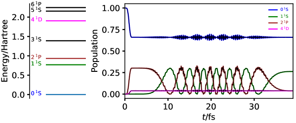
Figure 1: Energy-level populations computed with the aug-cc-pVTZ basis set through CCLR projectors plotted as functions of time for He exposed to two consecutive laser pulses, the first resonant with the $0^{1}\text{S}\to 2^{1}\text{P}$ transition and the second resonant with the $2^{1}\text{P}\to 1^{1}\text{S}$ transition, with peak intensity $87.7\,\text{TW/cm}^{2}$. The black curves show the populations during the TDFCI simulation.

The first sinusoidal laser pulse, applied at $t_{0}=0\,\text{a.u.}$, is resonant with the $0^{1}\text{S}\to 2^{1}\text{P}$ transition at $\omega_{0}=0.932\,\text{a.u.}$ and has peak intensity $87.7\,\text{TW/cm}^{2}$ (${\cal E}_{0}=0.05\,\text{a.u.}$) with a duration of $10$ optical cycles ($t_{d}=67.41\,\text{a.u.}=1.63\,\text{fs}$). The second sinusoidal pulse, applied immediately after the first pulse, is resonant with the $2^{1}\text{P}\to 1^{1}\text{S}$ transition at $\omega_{0}=0.163\,\text{a.u.}$ at the same peak intensity as the first pulse with a duration of $40$ optical cycles ($t_{d}=1545.19\,\text{a.u.}=37.38\,\text{fs}$). Both lasers are polarized along the $z$-axis with constant phase $\phi(t)=0$. The ground and excited levels are dominated by the electron configurations $1\text{s}^{2}$ (ground state, $0^{1}\text{S}$), $1\text{s}^{1}2\text{s}^{1}$ ($1^{1}\text{S}$), and $1\text{s}^{1}2\text{p}^{1}$ ($2^{1}\text{P}$).

The right panel of Fig. 1 shows the total energy-level populations computed using the CCLR projector as a function of time during the application of the two consecutive laser pulses. Energy levels that are never populated above $0.01$ are excluded. The level populations are computed by summing up populations of all states belonging to each energy level, thus avoiding ambiguities arising from the arbitrariness of the basis of a degenerate subspace. As expected, the first laser pulse causes significant population of the $2^{1}\text{P}$ energy level. The high-lying $4^{1}\text{D}$ level, which is dominated by the $1\text{s}^{1}3\text{d}^{1}$ electron configuration and located $0.972\,\text{a.u.}$ above the $2^{1}\text{P}$ level, also becomes populated towards the end of the first pulse due to the dipole-allowed transition $2^{1}\text{P}\to 4^{1}\text{D}$. The length-gauge oscillator strength of this transition is $f=0.484$ compared with $f=0.355$ for the $0^{1}\text{S}\to 2^{1}\text{P}$ transition. The population of the $4^{1}\text{D}$ level is still modest, however, since the transition can only occur once the $2^{1}\text{P}$ level is significantly populated.

The second pulse induces several cycles of Rabi oscillations between the $2^{1}\text{P}$ and $1^{1}\text{S}$ levels. The Rabi oscillations are slightly perturbed by weak transitions between the $2^{1}\text{P}$ level and the $0^{1}\text{S}$ ground state, as witnessed by the increasing oscillation of the ground-state population when the population of the $2^{1}\text{P}$ level is close to its maximum value. We also observe an even weaker perturbation caused by the higher-lying $4^{1}\text{D}$ level. The CCLR populations agree both with TDFCI populations and with EOMCC populations: the RMS deviation for the entire simulation is $10^{-3}$ between the CCLR and TDFCI populations and $3\times 10^{-7}$ between the CCLR and EOMCC populations. We have previously demonstrated that discrepancies with TDFCI simulations for the He atom can be reduced by tightening computational parameters such as convergence thresholds and, most importantly, by reducing the time step of the numerical integration ³⁰. We thus ascribe the small discrepancies between the CCLR and TDFCI populations to the rather coarse discretization ($\Delta t=0.1\,\text{a.u.}$) employed in the numerical integration scheme, and conclude that the proposed CCLR and EOMCC projectors behave correctly in the FCI limit.

It is of interest to compare the TDCCSD simulation with a much simpler model based on an eigenstate expansion propagated according to eq. (7). Letting $\ket{n},n=0,1,2,\cdots,14$, represent the stationary states computed with CCSD linear response theory, all we need to integrate eq. (7) in the presence of external laser pulses of the form (72) is the dipole matrix in the energy eigenbasis. This model is essentially identical to that employed by Sonk et al. ⁸⁴, except that we use CCSD linear and quadratic response theory rather than EOMCCSD theory to build the dipole matrix. (Note, however, that the CCSD response and EOMCCSD approaches yield identical results for He.) It is also similar to the EOMCCSD model employed by Luppi and Head-Gordon ⁸⁵, who propagated both bra and ket states.

The only obstacle is that the “right” and “left” transition moments from CC response theory, cf. eqs. (54) and (55), are not related by complex conjugation, yielding a spurious nonhermitian dipole matrix. Sonk et al. ⁸⁴ and Luppi and Head-Gordon ⁸⁵ circumvented this issue by only using the hermitian part of the matrix. In the present case, due to symmetry, the CCSD electric-dipole transition moments are either zero or may be chosen parallel to one of the three Cartesian axes, making it easy to define the off-diagonal dipole matrix elements as the negative square root of the dipole transition strength (cf. eq. (56) with $B=C$ a Cartesian component of the position operator). With the dipole matrix thus constructed for the $14$ states, we have integrated eq. (7) with the initial condition $C_{n}(t=0)=\delta_{n0}$, and the same consecutive laser pulses as in the He/aug-cc-pVTZ TDCCSD simulations. The Gauss-Legendre integrator was used with the same parameters and time step.

The RMS population deviation between the model and the full TDCCSD simulations is about twice that between the TDFCI and TDCCSD simulations. The maximum absolute deviation is an order of magnitude greater ($0.02$ versus $0.002$), however, indicating that a potentially large number of states, including states above the ionization energy, may be required for the simple model to agree quantitatively with full TDCCSD simulations in general.

Moving away from the FCI limit, we repeat the study of excited-state Rabi oscillations for the Be atom with the aug-cc-pVDZ basis set. The integration parameters were the same as those used for He above. The ground- and excited-state energy levels shown in the left panel of Fig. 2 were computed using CCSD linear response theory. In total, $21$ excited states were computed and the CCSD excitation energies agree with those of FCI theory to within $3\times 10^{-4}\,\text{a.u.}$. Several of the computed excited states lie above the ionization energy, which is estimated to be $0.341\,\text{a.u.}$ using the total ground-state energy difference between the neutral and ionized atom at the (spin unrestricted) CCSD/aug-cc-pVDZ level of theory ⁸³. The high-lying excited states are retained in order to compare with regular TDFCI simulations with the same basis set.

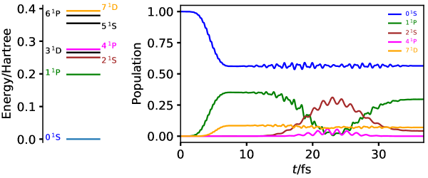
Figure 2: Energy-level populations computed with the aug-cc-pVDZ basis set through CCLR projectors plotted as functions of time for Be exposed to two consecutive laser pulses, the first resonant with the $0^{1}\text{S}\to 1^{1}\text{P}$ transition and the second resonant with the $1^{1}\text{P}\to 2^{1}\text{S}$ transition, with peak intensity $0.877\,\text{TW/cm}^{2}$.

The first sinusoidal laser pulse, applied at $t_{0}=0\,\text{a.u.}$, is resonant with the $0^{1}\text{S}\to 1^{1}\text{P}$ transition at $\omega_{0}=0.198\,\text{a.u.}$ and has peak intensity $0.877\,\text{TW/cm}^{2}$ (${\cal E}_{0}=0.005\,\text{a.u.}$) with a duration of $10$ optical cycles ($t_{d}=316.93\,\text{a.u.}=7.64\,\text{fs}$). The second sinusoidal pulse, applied immediately after the first pulse, is resonant with the $1^{1}\text{P}\to 2^{1}\text{S}$ transition at $\omega_{0}=0.0522\,\text{a.u.}$ at the same peak intensity as the first pulse with a duration of $10$ optical cycles ($t_{d}=1204.59\,\text{a.u.}=29.14\,\text{fs}$). Both lasers are polarized along the $z$-axis with constant phase $\phi(t)=0$. The ground and excited levels are dominated by the electron configurations $1\text{s}^{2}2\text{s}^{2}$ (ground state, $0^{1}\text{S}$), $1\text{s}^{2}2\text{s}^{1}2\text{p}^{1}$ ($1^{1}\text{P}$), and $1\text{s}^{1}2\text{s}^{1}3\text{s}^{1}$ ($2^{1}\text{S}$).

The right panel of Fig. 2 shows the total energy-level populations computed using the CCLR projector as a function of time during the application of the two consecutive laser pulses. Energy levels that are never populated above $0.01$ are excluded. The first laser pulse causes significant population of the $1^{1}\text{P}$ energy level by excitation from the ground state (oscillator strength $f=0.478$), although the transition is quenched by further excitation to the high-lying $7^{1}\text{D}$ level from the $1^{1}\text{P}$ level ($f=0.685$). The $7^{1}\text{D}$ level, which is dominated by the $1\text{s}^{2}2\text{s}^{1}3\text{d}^{1}$ electron configuration, is located $0.195\,\text{a.u.}$ above the $1^{1}\text{P}$ level and, hence, the $1^{1}\text{P}\to 7^{1}\text{D}$ transition is nearly resonant with the first laser. Consequently, the $7^{1}\text{D}$ level population increases once sufficient population of the $1^{1}\text{P}$ level is achieved towards the end of the first pulse. The second pulse induces a single-cycle Rabi oscillation between the $1^{1}\text{P}$ and $2^{1}\text{S}$ levels ($f=0.118$), which is quite significantly perturbed by the transition between the $2^{1}\text{S}$ and $4^{1}\text{P}$ levels ($f=0.211$). The population of the $4^{1}\text{P}$ level drops to zero as the Rabi oscillation enters the final stage where the population of the $2^{1}\text{S}$ level decreases.

The CCLR populations are in close agreement with TDFCI populations and with EOMCC populations: the RMS deviation for the entire simulation is $7.4\times 10^{-3}$ between the CCLR and TDFCI populations and $9.1\times 10^{-5}$ between the CCLR and EOMCC populations.

Increasing the basis set to aug-cc-pVTZ, the CCSD levels, the higher-lying ones in particular, move down in energy as seen by comparing the left panel of Fig. 3 with that of Fig. 2.

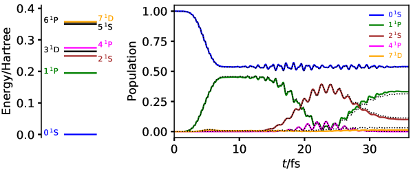
Figure 3: Energy-level populations computed with the aug-cc-pVTZ basis set through CCLR projectors plotted as functions of time for Be exposed to two consecutive laser pulses, the first resonant with the $0^{1}\text{S}\to 1^{1}\text{P}$ transition and the second resonant with the $1^{1}\text{P}\to 2^{1}\text{S}$ transition, with peak intensity $0.877\,\text{TW/cm}^{2}$. The dotted lines show the populations obtained using a simplified eigenstate expansion (see text) with the $22$ states forming the $8$ energy levels of the left panel included.

The right panel of Fig. 3 shows the variation of the level populations as the Be atom is exposed to the same sinusoidal laser pulses as in Fig. 2, albeit with the carrier frequencies adjusted to match the $0^{1}\text{S}\to 1^{1}\text{P}$ and $1^{1}\text{P}\to 2^{1}\text{S}$ transitions at $\omega_{0}=0.195\,\text{a.u.}$ and $\omega_{0}=0.0539\,\text{a.u.}$, respectively. The duration is $10$ optical cycles for each pulse, as above. The populations obtained from the CCLR and EOMCC projectors are vitually identical, with an overall RMS deviation of $1.6\times 10^{-4}$.

The lowering of the $7^{1}\text{D}$ level, which is now $0.162\,\text{a.u.}$ above the $1^{1}\text{P}$ level, implies that the probability of the $1^{1}\text{P}\to 7^{1}\text{D}$ transition ($f=0.648$) diminishes, resulting in very low population of the $7^{1}\text{D}$ level and increased population of the $1^{1}\text{P}$ level (compared with the aug-cc-pVDZ simulation) during the first pulse. Although the populations of the states involved thus are different, the perturbed Rabi oscillation induced by the second pulse is essentially the same as in Fig. 2.

While a full TDFCI simulation is too costly with the aug-cc-pVTZ basis set, we compare with the much simpler model introduced for He above. We use the same consecutive laser pulses and the Gauss-Legendre integrator with the same parameters as in the Be/aug-cc-pVTZ TDCCSD simulation for the model simulation with $22$ states included.

The resulting energy-level populations, plotted as dotted lines in Fig. 3, are remarkably similar to the full TDCCSD results. The maximum absolute deviations between the model and TDCCSD populations are just $15\%$ for the $1^{1}\text{P}$ level, $2\%$ for the $2^{1}\text{S}$ and $7^{1}\text{D}$ levels, and below $1\%$ for the remaining levels, including the ground state. Such good results can only be expected from the simple model when all, or very nearly all, participating CCSD states are included. How many states are needed will in general be very hard to estimate a priori.

4.2 Control by chirped laser pulses

Control by shaped laser pulses is an important challenge to theoretical simulations and requires information about population of energy levels. For the LiH molecule described with the aug-cc-pVDZ basis set, which is small enough to allow TDFCI reference simulations, we use chirped sinusoidal laser pulses to further test the proposed CCLR and EOMCC projectors within TDCCSD simulations. The laser pulses are polarized along the $x$-axis, perpendicular to the molecular axis, and the duration is kept fixed at $t_{d}=378.4\,\text{a.u.}=9.152\,\text{fs}$, corresponding to $10$ optical cycles of radiation resonant with the lowest-lying electric-dipole allowed transition from the ground state, the $x$-polarized ${}^{1}\Sigma^{+}\to\,^{1}\Pi$ transition at $\omega_{0}=0.166\,\text{a.u.}$. The laser pulses are turned on at $t_{0}=0\,\text{a.u.}$ with peak intensity $3.51\,\text{TW/cm}^{2}$ (${\cal E}_{0}=0.01\,\text{a.u.}$). The oscillator strength of this transition is estimated to be $f=0.208$ by CCSD linear response theory with the aug-cc-pVDZ basis set. The phase of the laser pulse is defined such that the instantaneous frequency is

$$\omega(t)=\omega_{0}+b\left(t-\frac{t_{d}}{3}\right)$$ (78)

and the chirp rate $b$ is varied between $-0.513\,\text{fs}^{-2}$ and $+0.513\,\text{fs}^{-2}$. A few such laser pulses with different chirp rates are shown in Fig. 4.

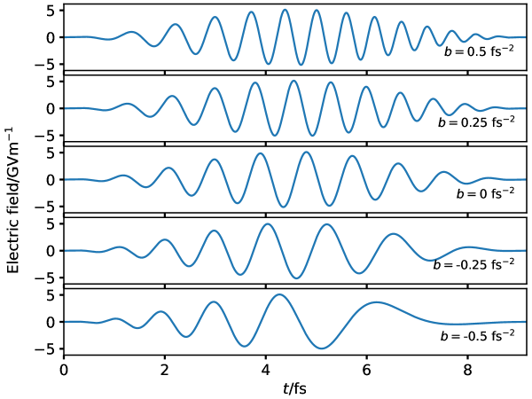
Figure 4: Laser pulses with different chirp rates.

The $31$ lowest-lying states, organized into $21$ energy levels in the left panel of Fig. 5, were computed with CCSD linear response theory (aug-cc-pVDZ basis) and used to construct CCLR and EOMCC projectors for the simulations.

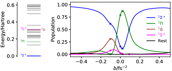
Figure 5: Final population of CCSD energy levels, computed with the CCLR projector, as a function of chirp rate for LiH with the aug-cc-pVDZ basis set. The squares mark reference populations from TDFCI simulations.

The highest-lying energy level is $0.603\,\text{a.u.}$ above the ground state, well beyond the ionization energy estimated by CCSD/aug-cc-pVDZ total-energy difference to be $0.281\,\text{a.u.}$ ⁸³. The most important energy levels in the simulations are marked by their term symbols. These states are all predominantly single-excited states, with at least $90\%$ contribution from singles in the EOMCC excitation amplitudes. While the ${}^{1}\Pi$ level at $0.166\,\text{a.u.}$ is well below the estimated ionization energy, the ${}^{1}\Delta$ and ${}^{1}\Sigma^{+}$ levels at $0.291\,\text{a.u.}$ and $0.312\,\text{a.u.}$, respectively, are slightly above. With $x$-polarized laser pulses, one-photon transitions from the ground state to the ${}^{1}\Delta$ and ${}^{1}\Sigma^{+}$ levels are electric-dipole forbidden, implying that these excited levels can only become populated by nonlinear optical processes.

The final populations of these levels, computed immediately after the interaction with the chirped sinusoidal laser pulse, are shown in the right panel of Fig. 5 along with a few reference TDFCI results. The TDCCSD (and TDFCI) equations of motion were integrated using the sixth order ($s=3$) Gauss-Legendre integrator with time step $\Delta t=0.1\,\text{a.u.}$ and convergence threshold $10^{-6}$. The sum of the populations of the remaining $27$ energy levels is labelled “Rest” and is seen to be insignificant for all but the most up- or down-chirped pulses. At $b=0\,\text{fs}^{-2}$, the pulse is resonant with the ground-state ${}^{1}\Sigma^{+}\to\,^{1}\Pi$ transition and, therefore, other levels are hardly populated. The maximum population of the ${}^{1}\Pi$ level is observed at a slightly up-chirped pulse (at $b=0.023\,\text{fs}^{-2}$), which prevents further excitation from the ${}^{1}\Pi$ level to the higher-lying ${}^{1}\Sigma^{+}$ and ${}^{1}\Delta$ levels. As the chirp rate increases, the laser pulse becomes increasingly off-resonant and the ground-state population increases.

The population of the excited ${}^{1}\Sigma^{+}$ level and, in particular, of the ${}^{1}\Delta$ level increases with moderately down-chirped pulses due to transitions from the ${}^{1}\Pi$ level, whose probability increases as the laser frequency decreases. At $b=-0.102\,\text{fs}^{-2}$, the population of the ${}^{1}\Pi$ level is just $9.3\times 10^{-4}$, while the excited ${}^{1}\Sigma^{+}$ and ${}^{1}\Delta$ populations are close to their maximum values. These nonlinear optical processes can easily be understood by studying the populations during interaction with the laser pulse in Fig. 6.

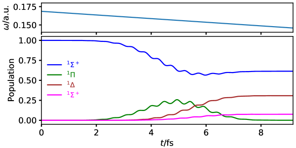
Figure 6: Energy-level populations computed with the aug-cc-pVDZ basis set through CCLR projectors plotted as functions of time for LiH exposed to a down-chirped laser pulse with chirp rate $b=-0.102\,\text{fs}^{-2}$. The instantaneous frequency of the laser pulse is shown in the top panel.

During the first half of the pulse, the instantaneous laser frequency is nearly resonant with the ground-state ${}^{1}\Sigma^{+}\to\,^{1}\Pi$ transition at $0.166\,\text{a.u.}$ ($f=0.207$), causing the population of the ${}^{1}\Pi$ level to increase. As the instantaneous frequency decreases, it comes closer to the transition frequencies of the ${}^{1}\Pi\to\,^{1}\Delta$ and ${}^{1}\Pi\to\,^{1}\Sigma^{+}$ transitions at $0.138\,\text{a.u.}$ and $0.146\,\text{a.u.}$, respectively. Although the instantaneous frequency is closer to the ${}^{1}\Pi\to\,^{1}\Sigma^{+}$ transition than to the ${}^{1}\Pi\to\,^{1}\Delta$ transition, the latter level is considerably more populated. This is explained by the difference in oscillator strength for these transitions: $f=0.363$ for the ${}^{1}\Pi\to\,^{1}\Delta$ transition compared with $f=0.076$ for the ${}^{1}\Pi\to\,^{1}\Sigma^{+}$ transition.

The differences between the EOMCC and CCLR projectors are, again, utterly insignificant, the typical RMS population deviation beetween them being approximately $10^{-5}$ regardless of chirp rate. As can be seen from Fig. 5, the TDCCSD simulations are in excellent agreement with TDFCI results. This is not unexpected, since all states participating in the dynamics are single-excited states. The maximum absolute deviation in the $30$ excitation energies, including the excited states with significant double-excited character (down to $11\%$ singles contribution in the EOMCC excitation amplitudes), between CCSD linear response theory and FCI theory is just $0.0013\,\text{a.u.}$.

4.3 Dynamics involving double-excited states

In general, CCSD linear response theory performs poorly for states dominated by double-excited determinants relative to the HF ground state. For such states, excitation-energy errors are typically an order of magnitude greater than for single-excited states ^{86, 87}, roughly $0.01\,\text{a.u.}$ for double-excited states compared with $0.001\,\text{a.u.}$ for single-excited states of small molecules where FCI results are available ⁸⁷. In all examples presented above, the states participating significantly in the dynamics are all single-excitation dominated, explaining the close agreement observed between TDFCI and TDCCSD simulations.

With a ground-state wave function dominated by the HF ground-state determinant, one-photon transitions to excited states dominated by double-excited determinants are either electric-dipole forbidden or only weakly allowed. Accordingly, we expect double-excited states to influence laser-driven many-electron dynamics mainly through nonlinear optical processes. In order to test the influence on TDCCSD dynamics, we consider the CH⁺ molecule, which is a classic example of the relatively poor performance of CCSD linear response and EOMCCSD theory for such states, see, for example, Refs. 88, 89, 90.

The ${}^{1}\Sigma^{+}$ ground state of CH⁺ is dominated by the $1\sigma^{2}2\sigma^{2}3\sigma^{2}$ electron configuration with some non-dynamical correlation contribution from the double-excited $1\sigma^{2}2\sigma^{2}1\pi^{2}$ configuration. The two lowest-lying excited states form the ${}^{1}\Pi$ energy level and are dominated by the single-excited $1\sigma^{2}2\sigma^{2}3\sigma^{1}1\pi^{1}$ configuration. The three subsequent states form two energy levels, ${}^{1}\Delta$ and ${}^{1}\Sigma^{+}$, and are almost purely double-excited states stemming from the $1\sigma^{2}2\sigma^{2}1\pi^{2}$ electron configuration. Transitions from the ground state to these levels are either electric-dipole forbidden (${}^{1}\Delta$) or very weak with oscillator strengths on the order of $10^{-3}$. Significant population of these levels, therefore, can only be achieved through nonlinear optical processes, requiring rather intense laser pulses.

In order to make TDFCI simulations feasible for CH⁺, we use a reduced aug-cc-pVDZ basis set where the diffuse $p$ funtions on hydrogen and the diffuse $d$ functions on carbon have been removed. While removing these diffuse functions has little effect on the $5$ lowest CCSD linear response excitation energies (RMS deviation $0.001\,\text{a.u.}$), the effect is significant on the following $25$ excitation energies with an RMS deviation of $0.021\,\text{a.u.}$. The $31$ lowest-lying states, forming $21$ energy levels, computed with CCSD linear response and FCI theory are shown in the left panel of Fig. 7.

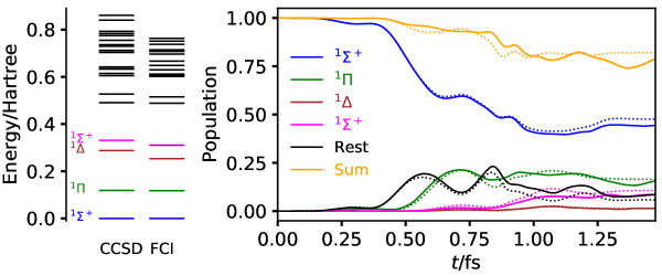
Figure 7: TDCCSD (full curves) energy-level populations computed with the reduced aug-cc-pVDZ basis set through CCLR projectors plotted as functions of time for CH⁺. The dotted curves are populations computed with TDFCI theory. The total population of the black levels in the left panel is labelled “Rest” in the right panel. The curves labeled “Sum” are the total population of all $21$ levels computed at the CCSD and FCI levels of theory.

The ionization energy of CH⁺ is estimated to be $0.878\,\text{a.u.}$ using ionization-potential EOMCCSD theory and $0.876\,\text{a.u.}$ using FCI theory with the 6-31G* basis set. ⁹¹ Hence, all computed states are below the estimated ionization energies.

We expose the CH⁺ ion to a sinusoidal laser pulse with intensity $2654\,\text{TW/cm}^{2}$ (${\cal E}_{0}=0.275\,\text{a.u.}$) and carrier frequency $\omega_{0}=0.212\,\text{a.u.}$, which is resonant with the ${}^{1}\Pi\to\,^{1}\Sigma^{+}$ transition between excited states at the CCSD level of theory. The pulse is polarized along the $y$-axis, perpendicular to the bond axis, with duration $t_{d}=66.7\,\text{a.u.}=1.61\,\text{fs}$, corresponding to $2.05$ optical cycles. The TDCCSD and TDFCI equations of motion were integrated with the sixth-order ($s=3$) Gauss-Legendre integrator with time step $\Delta t=0.05\,\text{a.u.}$ and convergence threshold $10^{-6}$. The resulting energy-level populations are presented in the right panel of Fig. 7. Populations of the $4$ lowest-lying levels, including the ground state, are shown along with the sum of the populations of the remaining $17$ levels, labelled “Rest”. The total population of all computed levels is labelled “Sum”.

The effect of poorly described double-excited states at the CCSD level of theory is evident, although we do observe a qualitative agreement with FCI theory. We first note that the $21$ levels included in the analysis only account for about $80\%$ of the norm of the FCI wave function at the end of the pulse, implying that a physically correct description must also take ionization processes into account. This, of course, is not surprising, considering the high intensity of the pulse. The TDFCI and TDCCSD populations agree reasonably well during the first $0.75\,\text{fs}$ of the simulation, wheras the TDCCSD errors increase as the simulation progresses.

Involving a large number of states, the dynamics is considerably more complex than the dynamics of the cases presented above. For simplicity, we use a classification of the $30$ excited states based on their single- or double-excitation character. Excited states with more than $90\%$ contribution from singles in the EOMCCSD amplitude norm are classified as single-excited states, while states with less than $10\%$ singles contribution are classified as double-excited states. States with $10$–$90\%$ singles contribution are mixed states, classified as singles-dominated ($>50\%$ singles contribution) or doubles-dominated ($<50\%$ singles contribution). Thus, the $30$ excited CCSD states can be grouped into $7$ single-excited states, $4$ singles-dominated states, $5$ doubles-dominated states, and $14$ double-excited states. The total population of each class of states is presented in Fig. 8.

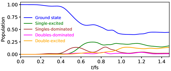
Figure 8: Population of different classes of CCSD states for CH⁺ with the reduced aug-cc-pVDZ basis set.

After about $0.4\,\text{fs}$ the laser pulse induces transitions from the ground state into singles-dominated states, followed by transitions (from both the ground state and the singles-dominated excited states) into single-excitation states. Double-excited or doubles-dominated states are barely populated at this stage, explaining the reasonable agreement with TDFCI populations. Roughly half-way through the simulation, double-excited states and, to a smaller extent, doubles-dominated states become populated, mainly due to transitions from singles-dominated states. As soon as these processes occur, the agreement between TDCCSD and TDFCI deteriorates.

4.4 Population conservation

As discussed in Section 2.6, stationary-state populations in the absence of external forces are strictly conserved in the FCI limit but may vary when the cluster operators are truncated. In order to investigate the breaking of the population conservation law within TDCCSD theory, we have conducted simple numerical experiments with several of the systems presented above. We apply the same sinusoidal laser pulses as above but continue the propagation after the pulses have been turned off, recording stationary-state population using the CCLR and EOMCC projectors.

Figure 9 shows the conservation of TDCCSD populations after the laser pulses have been turned off for the He atom with the aug-cc-pVTZ basis set.

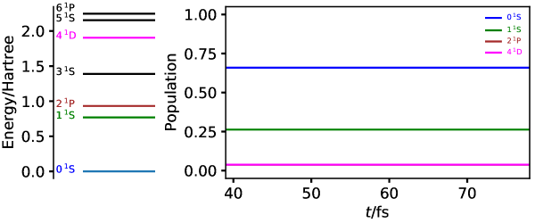
Figure 9: Conservation of TDCCSD energy-level populations after the laser pulses have been turned off for the He atom with the aug-cc-pVTZ basis set. The populations were computed using the CCLR projector.

A maximum absolute deviation in the populations of $1.5\times 10^{-3}$ is observed for the $1^{1}\text{S}$ and $2^{1}\text{P}$ levels, whereas the deviations for the remaining levels are at least one order of magnitude smaller. These deviations from exact conservation are likely caused by the discretization of the numerical integration.

Slightly larger deviations from strict conservation are observed for the Be atom with the aug-cc-pVTZ basis set in Fig. 10.

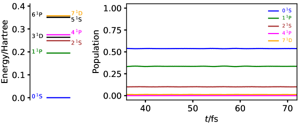
Figure 10: Conservation of TDCCSD energy-level populations after the laser pulses have been turned off for the Be atom with the aug-cc-pVTZ basis set. The populations were computed using the CCLR projector.

The maximum absolute deviation of $0.005$ is observed for the $1^{1}\text{P}$ level. Caused by the truncation of the cluster operators in conjunction with discretization, this deviation is thrice greater than that observed for He above. Only a weak oscillatory behavior is observed, indicating that the states involved in the dynamics are very well approximated at the CCSD level of theory.

Energy-level populations for LiH during and after interaction with a chirped laser pulse are plotted Fig. 11.

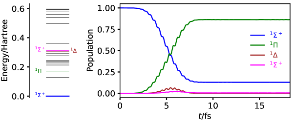
Figure 11: Conservation of TDCCSD energy-level populations of LiH after interaction with a chirped laser pulse with chirp rate $b=0.03078\,\text{fs}^{-2}$. The populations were computed using the CCLR projector and the aug-cc-pVDZ basis set.

The chirp rate $b=0.03078\,\text{fs}^{-2}$ yields a final state dominated by the ${}^{1}\Pi$ level and the populations remain constant to an excellent approximation after the interaction ceases. The maximum absolute deviation is observed for the ${}^{1}\Pi$ level and is on par with that observed for He atom: $1.7\times 10^{-3}$.

As we saw above, the TDCCSD method is a much poorer approximation to TDFCI theory in the case of CH⁺, where double-excited states participate significantly in the dynamics. On these grounds, we expect a much poorer conservation of energy-level populations after interaction with the laser pulse and, indeed, large deviations can be seen in Fig. 12.

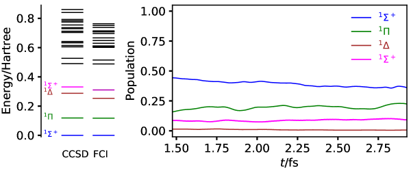
Figure 12: Conservation of TDCCSD energy-level populations of CH⁺ after interaction with a laser pulse. The populations were computed using the CCLR projector and the reduced aug-cc-pVDZ basis set.

The depletion of the ground state appears to continue after the pulse and irregular weakly oscillatory behavior is observed for the ${}^{1}\Pi$ level with a maximum absolute deviation of $0.072$, which is an order magnitude greater than the devations found for He, Be, and LiH above. The double-excited ${}^{1}\Delta$ and ${}^{1}\Sigma$ levels show maximum absolute deviations of $0.009$ and $0.019$, respectively.

4.5 Pump spectrum of LiF

Skeidsvoll et al. recently reported a theoretical TDCCSD study of transient X-ray spectroscopy of the LiF molecule. ³⁸ They applied a pump-probe laser setup with an optical pump pulse resonant with the lowest-lying dipole-allowed transition from the ground state, followed, at various delays, by an X-ray probe pulse resonant with the first dipole-allowed core excitation. The resulting time-resolved spectra were interpreted by means of excitation energies from EOMCC theory and core-valence separated EOMCC theory. ⁹² The pump absorption spectrum reported in Fig. 7 of Ref. 38 contains weak unassigned features, one weak absorption above the two low-lying valence excitations and two very weak features below, which the authors speculated were due to two-photon absorptions. We will now use the EOMCC and CCLR projectors to investigate what might cause these weak features of the pump absorption spectrum. We use the same basis set, denoted aug-cc-p(C)VDZ, as in Ref. 38: the aug-cc-pVDZ basis set for Li and the aug-cc-pCVDZ basis set for F. The closed-shell TDCCSD equations of motion were integrated using the sixth-order ($s=3$) Gauss-Legendre integrator with time step $\Delta t=0.025\,\text{a.u.}=0.60\,\text{as}$ and convergence threshold $10^{-6}$ for the fix-point iterations.

Initially in the ground state, we expose the LiF molecule to a shortened but otherwise identical $z$-polarized Gaussian laser pulse to that in Ref. 38, with field strength ${\cal E}_{0}=0.01\,\text{a.u.}$ (peak intensity $I=3.51\,\text{TW/cm}^{2}$), carrier frequency $\omega_{0}=0.2536\,\text{a.u.}$, and Gaussian RMS width $\sigma=20\,\text{a.u.}$. The shortening consists in choosing the central time $t_{0}=80\,\text{a.u.}$ (compared with $t_{0}=160\,\text{a.u.}$ in Ref. 38) and $N=4$ (compared with $N=8$ in Ref. 38). This implies that the electric-field amplitude jumps from zero to $3.3\times 10^{-6}\,\text{a.u.}$ at $t=0\,\text{a.u.}$ and from $3.3\times 10^{-6}\,\text{a.u.}$ to zero at $t=160\,\text{a.u.}$, whereas virtually no discontinuities can be observed with the pulse parameters used in Ref. 38 (they are on the order of $10^{-16}\,\text{a.u.}$). Since the pump pulse is quite weak, the effects of these discontinuities on the populations are negligible, as can readily be verified using a simple eigenstate expansion analogous to the one used for He and Be in Section 4.1.

Our TDCCSD results are presented in Fig. 13. The first $30$ excited states ($20$ energy levels, left panel of Fig. 13) are all single-excitation dominated states, with $94.9$–$95.4\%$ singles contribution to the norm of the EOMCCSD amplitudes. The highest-lying states are somewhat above the first ionization energy of LiF, which we estimate to be about $0.4\,\text{a.u.}$ ($11\,\text{eV}$) based on data available in Ref. 83.

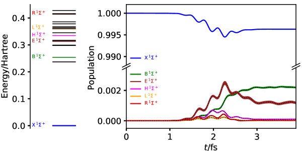
Figure 13: TDCCSD energy-level populations computed with the aug-cc-p(C)VDZ basis set through CCLR (colored full curves) and EOMCC (black dotted curves) projectors plotted as functions of time for LiF. The $20$ lowest-lying CCSD energy levels (corresponding to $30$ states) are shown in the left panel with participating levels counted alphabetically as in Ref. 38.

The modest intensity of the pump pulse results in fairly little excitation from the ground state, well within reach of a perturbation-theoretical (Fermi’s golden rule) treatment. In agreement with Ref. 38, the projectors predict the absorption to be dominated by the B$\,{}^{1}\Sigma^{+}$ and E$\,{}^{1}\Sigma^{+}$ states. The final population of the latter is roughly $53\%$ of the former, in good agreement with the relative intensities of the pump spectrum reported in Fig. 7 of Ref. 38. The population of the E$\,{}^{1}\Sigma^{+}$ state reaches its maximum value $0.0025$ at $t=2.26\,\text{fs}$; at the same time the ground-state population reaches its minimum value $0.9945$, indicating that the ensuing decay of the E$\,{}^{1}\Sigma^{+}$ population is caused by transition back to the ground state.

The weak feature at higher frequency (at about $9.1\,\text{eV}$) in the pump spectrum of Ref. 38 is seen to be consistent with one-photon transition from the ground state to the H$\,{}^{1}\Sigma^{+}$ state, whose final population is about $5\%$ of that of the B$\,{}^{1}\Sigma^{+}$ state. As speculated by Skeidsvoll et al. ³⁸, the two very weak features below the B$\,{}^{1}\Sigma^{+}$ line in Ref. 38 are indeed seen to arise from direct two-photon absorptions from the ground state to the L$\,{}^{1}\Sigma^{+}$ and R$\,{}^{1}\Sigma^{+}$ states. The only alternative explanation would be excitations between excited states, but this mechanism can almost certainly be ruled out, since the population of these states starts before other excited levels are significantly populated and since no other excited states are depleted as the populations of these states increase.

Although the CCLR and EOMCC populations largely agree with an overall RMS deviation of $7\times 10^{-6}$, the CCLR populations show spurious high-frequency oscillations in Fig. 13. The oscillations are caused by the off-diagonal contributions from $\bra{\breve{\Psi}_{n}}$ (eq. (49)) to the CCLR projector (eq.(47)). While these contributions are required to ensure proper size-intensivity of one-photon transition moments, they also cause nonorthogonality of the CCLR excited-state representation as expressed by eq. (57). Since the CCLR and EOMCC projectors provided virtually identical results in the cases above, this observation serves as a recommendation of the EOMCC projector for the calculation of stationary-state populations.

Figure 14 depicts a normalized pump spectrum of LiF generated from the final EOMCC populations using

$$I(\omega)=\frac{S(\omega)}{\max_{\omega}S(\omega)},\qquad S(\omega)=\sum_{n}\frac{p_{n}(t_{\text{\scriptsize{final}}})}{\pi}\frac{\gamma}{(\omega-\Delta E_{n})^{2}+\gamma^{2}}$$ (79)

where $\gamma=0.01\,\text{eV}$ is an artifical Lorentzian broadening of the excited levels.

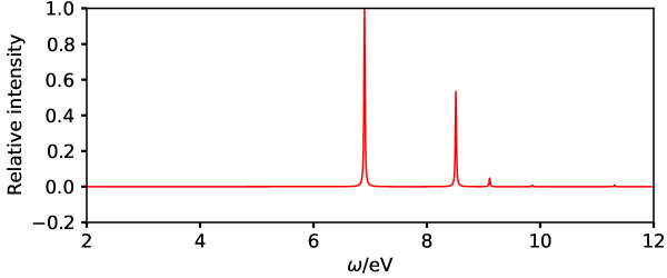
Figure 14: Pump spectrum of LiF generated from EOMCC populations assuming one-photon transitions from the ground state.

This approach implicitly assumes that the excited states only become populated through one-photon absorption from the ground state, thus excluding all nonlinear optical processes. The population-based pump spectrum agrees remarkably well with that reported by Skeidsvoll et al. ³⁸, which was properly generated from Fourier transformation of the induced dipole moment. This supports the conclusion that the low-frequency features are two-photon absorptions and further strengthens the confidence in the proposed EOMCC projector for the calculation of stationary-state populations in TDCC simulations.

5 Concluding remarks

We have proposed projectors for the interpretation of many-electron dynamics within TDCC theory in terms of the population of stationary states. Two conditions are used to define suitable projectors from CC linear response theory and from EOMCC theory: (i) the projector must reproduce the correct form of one-photon transition strengths and (ii) the projectors must yield populations that converge to the FCI results in the limit of untruncated cluster operators.

The CCLR and EOMCC projectors are tested numerically at the TDCCSD level of theory for the laser-driven dynamics in the He and Be atoms, and in the molecules LiH, CH⁺, and LiF. It is demonstrated that the populations provide valuable insight into the linear and nonlinear optical processes occcuring during the interaction of the electrons with laser pulses. For the He atom, it is verified numerically that the populations computed from both CCLR and EOMCC projectors agree with those computed from TDFCI simulations. For Be and LiH, the CCLR and EOMCC populations show excellent agreement with TDFCI populations, since the excited stationary states involved in the dynamics are dominated by single-excited Slater determinants. Such states are generally well described by CCSD theory. For CH⁺, we deliberately design the laser pulse such that double-excitation dominated states become populated, which reduces the agreement between TDFCI and TDCCSD populations. This is also reflected in studies of the conservation of populations after the laser pulses are turned off. Theoretically, the TDCC populations will only be strictly conserved in the FCI limit. Numerically, we find that they are nearly conserved as long as the participating stationary states are well approximated at the CCSD level of theory. Finally, for LiF, we use the CCLR and EOMCC projectors to explain unassigned weak features in a theoretical TDCCSD pump spectrum reported recently ³⁸.

Overall, the CCLR and EOMCC projectors yield very similar excited-state populations with typical RMS deviations on the order of $10^{-5}$. For LiF, however, we observe small-amplitude high-frequency oscillations of the excited-state populations computed with the CCLR projector. Originating from a contribution that vanishes in the FCI limit, we speculate that such oscillations may increase for larger and more complex systems where TDCCSD theory may be further from TDFCI theory. Not showing signs of such spurious behavior, the EOMCC projector appears more attractive than the CCLR projector. This has the added benefit that the additional response equations (51) need not be solved, thus making the EOMCC projectors less computationally demanding than the CCLR projectors.

These findings call for further research aimed at a fully consistent definition of excited states in CC theory, and work in this direction is in progress in our labs.

This work was supported by the Research Council of Norway (RCN) through its Centres of Excellence scheme, project number 262695, by the RCN Research Grant No. 240698, by the European Research Council under the European Union Seventh Framework Program through the Starting Grant BIVAQUM, ERC-STG-2014 grant agreement No. 639508, and by the Norwegian Supercomputing Program (NOTUR) through a grant of computer time (Grant No. NN4654K).

Appendix: the FCI limit

The CCLR projector, eq. (47) becomes identical to the EOMCC projector, eq. (33), in the FCI limit. To show this, we will now demonstrate that

$$\bra{\breve{\Psi}_{n}}=\bra{\bar{\Psi}_{n}}-{\cal R}^{n}_{0}\bra{\tilde{\Psi}_{0}}=0$$ (80)

in the FCI limit.

In the FCI limit, the EOMCC wave functions satisfy the time-independent Schrödinger equation and its hermitian conjugate,

$$H_{0}\ket{\Psi_{0}}=\ket{\Psi_{0}}E_{0}, H_{0}\ket{\Psi_{n}}=\ket{\Psi_{n}}E_{n}$$ (81)

$$\bra{\tilde{\Psi}_{0}}H_{0}=E_{0}\bra{\tilde{\Psi}_{0}}, \bra{\tilde{\Psi}_{n}}H_{0}=E_{n}\bra{\tilde{\Psi}_{n}}$$ (82)

where the ground- and excited-state wave functions constitute a biorthonormal set according to eqs. (39) and (40). The resolution-of-the-identity reads

$$\ket{\Psi_{0}}\bra{\tilde{\Psi}_{0}}+\sum_{n}\ket{\Psi_{n}}\bra{\tilde{\Psi}_{n}}=1$$ (83)

where $1$ is to be understood as the identity operator. To verify the resolution-of-the-identity, one simply inserts the definitions of the wave functions and exploits the biorthonormality of the Jacobian eigenvectors, eq. (37), along with the completeness of the underlying determinant basis.

According to eq. (51), the amplitudes $\bar{\cal M}^{n}_{\mu}$ can be recast as

$$\bar{\cal M}^{n}_{\mu} =-\sum_{\nu\gamma}{\cal R}^{n}_{\nu}F_{\nu\gamma}\left(\boldsymbol{A}+\Delta E_{n}\boldsymbol{1}\right)^{-1}_{\gamma\mu}$$

$$=-\sum_{m}\sum_{\nu\gamma}{\cal R}^{n}_{\nu}F_{\nu\gamma}{\cal R}^{m}_{\gamma}(\Delta E_{n}+\Delta E_{m})^{-1}{\cal L}^{m}_{\mu}$$

$$=-\sum_{m}\braket{\tilde{\Psi}_{0}}{[[H_{0},R_{n}],R_{m}]}{\Psi_{0}}(\Delta E_{n}+\Delta E_{m})^{-1}{\cal L}^{m}_{\mu}$$ (84)

where we have used eq. (37). Expanding the nested commutator and using eqs. (81), (82), (83), and (39) we find

$$\braket{\tilde{\Psi}_{0}}{[[H_{0},R_{n}],R_{m}]}{\Psi_{0}} =-(\Delta E_{n}+\Delta E_{m})\left(\braket{\tilde{\Psi}_{0}}{R_{n}R_{m}}{\Psi_{0}}-{\cal R}^{n}_{0}{\cal R}^{m}_{0}\right)$$

$$=-(\Delta E_{n}+\Delta E_{m})\braket{\tilde{\Psi}_{0}}{R_{n}\left(1-\ket{\Psi_{0}}\bra{\tilde{\Psi}_{0}}\right)R_{m}}{\Psi_{0}}$$

$$=-(\Delta E_{n}+\Delta E_{m})\braket{\tilde{\Psi}_{0}}{R_{n}}{\Psi_{m}}$$ (85)

giving

$$\bar{\cal M}^{n}_{\mu}=\sum_{m}\braket{\tilde{\Psi}_{0}}{R_{n}}{\Psi_{m}}{\cal L}^{m}_{\mu}$$ (86)

Hence,

$$\bra{\bar{\Psi}_{n}} =\sum_{\mu}\bra{\tilde{\Phi}_{\mu}}\bar{\cal M}^{n}_{\mu}\text{e}^{-T_{0}}-\bra{\tilde{\Psi}_{0}}R_{n}$$

$$=\sum_{m}\braket{\tilde{\Psi}_{0}}{R_{n}}{\Psi_{m}}\bra{\tilde{\Psi}_{m}}-\bra{\tilde{\Psi}_{0}}R_{n}$$

$$=\bra{\tilde{\Psi}_{0}}R_{n}\left(\sum_{m}\ket{\Psi_{m}}\bra{\tilde{\Psi}_{m}}-1\right)$$

$$=-\braket{\tilde{\Psi}_{0}}{R_{n}}{\Psi_{0}}\bra{\tilde{\Psi}_{0}}={\cal R}^{n}_{0}\bra{\tilde{\Psi}_{0}}$$ (87)

which shows that $\bra{\breve{\Psi}_{n}}=0$ in the FCI limit.

References

- Lépine et al. 2014 Lépine, F.; Ivanov, M. Y.; Vrakking, M. J. Attosecond molecular dynamics: Fact or fiction? Nat. Photon. 2014, 8, 195–204
- Li et al. 2020 Li, J.; Lu, J.; Chew, A.; Han, S.; Li, J.; Wu, Y.; Wang, H.; Ghimire, S.; Chang, Z. Attosecond science based on high harmonic generation from gases and solids. Nat. Commun. 2020, 11, 1–13
- Hassan et al. 2016 Hassan, M. T.; Luu, T. T.; Moulet, A.; Raskazovskaya, O.; Zhokhov, P.; Garg, M.; Karpowicz, N.; Zheltikov, A. M.; Pervak, V.; Krausz, F.; Goulielmakis, E. Optical attosecond pulses and tracking the nonlinear response of bound electrons. Nature 2016, 530, 66–70
- Runge and Gross 1984 Runge, E.; Gross, E. K. Density-functional theory for time-dependent systems. Phys. Rev. Lett. 1984, 52, 997–1000
- van Leeuwen 1999 van Leeuwen, R. Mapping from densities to potentials in time-dependent density-functional theory. Phys. Rev. Lett. 1999, 82, 3863–3866
- Ullrich 2012 Ullrich, C. A. Time-Dependent Density-Functional Theory; Oxford University Press: Oxford, 2012
- Li et al. 2020 Li, X.; Govind, N.; Isborn, C.; DePrince, A. E.; Lopata, K. Real-Time Time-Dependent Electronic Structure Theory. Chem. Rev. 2020, 120, 9951–9993
- Zanghellini et al. 2003 Zanghellini, J.; Kitzler, M.; Fabian, C.; Brabec, T.; Scrinzi, A. An MCTDHF Approach to Multielectron Dynamics in Laser Fields. Laser Phys. 2003, 13, 1064–1068
- Kato and Kono 2004 Kato, T.; Kono, H. Time-dependent multiconfiguration theory for electronic dynamics of molecules in an intense laser field. Chem. Phys. Lett. 2004, 392, 533–540
- Meyer et al. 2009 Meyer, H.-D., Gatti, F., Worth, G., Eds. Multidimensional Quantum Dynamics: MCTDH Theory and Applications; Wiley: Weinheim, Germany, 2009
- Hochstuhl et al. 2014 Hochstuhl, D.; Hinz, C. M.; Bonitz, M. Time-dependent multiconfiguration methods for the numerical simulation of photoionization processes of many-electron atoms. Eur. Phys. J. Special Topics 2014, 223, 177–336
- Sato and Ishikawa 2013 Sato, T.; Ishikawa, K. L. Time-dependent complete-active-space self-consistent-field method for multielectron dynamics in intense laser fields. Phys. Rev. A 2013, 88, 023402
- Miyagi and Madsen 2013 Miyagi, H.; Madsen, L. B. Time-dependent restricted-active-space self-consistent-field theory for laser-driven many-electron dynamics. Phys. Rev. A 2013, 87, 062511
- Miyagi and Madsen 2014 Miyagi, H.; Madsen, L. B. Time-dependent restricted-active-space self-consistent-field theory for laser-driven many-electron dynamics. II. Extended formulation and numerical analysis. Phys. Rev. A 2014, 89, 063416
- Bartlett and Musial 2007 Bartlett, R.; Musial, M. Coupled-cluster theory in quantum chemistry. Rev. Mod. Phys. 2007, 79, 291–352
- Hoodbhoy and Negele 1978 Hoodbhoy, P.; Negele, J. W. Time-dependent coupled-cluster approximation to nuclear dynamics. I. Application to a solvable model. Phys. Rev. C 1978, 18, 2380–2394
- Hoodbhoy and Negele 1979 Hoodbhoy, P.; Negele, J. W. Time-dependent coupled-cluster approximation to nuclear dynamics. II. General formulation. Phys. Rev. C 1979, 19, 1971–1982
- Schönhammer and Gunnarsson 1978 Schönhammer, K.; Gunnarsson, O. Time-dependent approach to the calculation of spectral functions. Phys. Rev. B 1978, 18, 6606–6614
- Dalgaard and Monkhorst 1983 Dalgaard, E.; Monkhorst, H. J. Some aspects of the time-dependent coupled-cluster approach to dynamic response functions. Phys. Rev. A 1983, 28, 1217–1222
- Arponen 1983 Arponen, J. Variational principles and linked-cluster exp S expansions for static and dynamic many-body problems. Ann. Phys. 1983, 151, 311–382
- Pigg et al. 2012 Pigg, D. A.; Hagen, G.; Nam, H.; Papenbrock, T. Time-dependent coupled-cluster method for atomic nuclei. Phys. Rev. C 2012, 86, 014308
- Huber and Klamroth 2011 Huber, C.; Klamroth, T. Explicitly time-dependent coupled cluster singles doubles calculations of laser-driven many-electron dynamics. J. Chem. Phys. 2011, 134, 054113
- Kvaal 2012 Kvaal, S. Ab initio quantum dynamics using coupled-cluster. J. Chem. Phys. 2012, 136, 194109
- Nascimento and DePrince 2016 Nascimento, D. R.; DePrince, A. E. Linear Absorption Spectra from Explicitly Time-Dependent Equation-of-Motion Coupled-Cluster Theory. J. Chem. Theory Comput. 2016, 12, 5834–5840
- Nascimento and DePrince 2017 Nascimento, D. R.; DePrince, A. E. Simulation of Near-Edge X-ray Absorption Fine Structure with Time-Dependent Equation-of-Motion Coupled-Cluster Theory. J. Phys. Chem. Lett 2017, 8, 2951–2957
- Nascimento and DePrince 2019 Nascimento, D. R.; DePrince, A. E. A general time-domain formulation of equation-of-motion coupled-cluster theory for linear spectroscopy. J. Chem. Phys. 2019, 151, 204107
- Koulias et al. 2019 Koulias, L. N.; Williams-Young, D. B.; Nascimento, D. R.; DePrince, A. E.; Li, X. Relativistic Real-Time Time-Dependent Equation-of-Motion Coupled-Cluster. J. Chem. Theory Comput. 2019, 15, 6617–6624
- Park et al. 2019 Park, Y. C.; Perera, A.; Bartlett, R. J. Equation of motion coupled-cluster for core excitation spectra: Two complementary approaches. J. Chem. Phys. 2019, 151, 164117
- Pedersen and Kvaal 2019 Pedersen, T. B.; Kvaal, S. Symplectic integration and physical interpretation of time-dependent coupled-cluster theory. J. Chem. Phys. 2019, 150, 144106
- Kristiansen et al. 2020 Kristiansen, H. E.; Schøyen, Ø. S.; Kvaal, S.; Pedersen, T. B. Numerical stability of time-dependent coupled-cluster methods for many-electron dynamics in intense laser pulses. J. Chem. Phys. 2020, 152, 071102
- Sato et al. 2018 Sato, T.; Pathak, H.; Orimo, Y.; Ishikawa, K. L. Time-dependent optimized coupled-cluster method for multielectron dynamics. J. Chem. Phys. 2018, 148, 051101
- Pathak et al. 2020 Pathak, H.; Sato, T.; Ishikawa, K. L. Time-dependent optimized coupled-cluster method for multielectron dynamics. II. A coupled electron-pair approximation. J. Chem. Phys. 2020, 152, 124115
- Pathak et al. 2020 Pathak, H.; Sato, T.; Ishikawa, K. L. Time-dependent optimized coupled-cluster method for multielectron dynamics. III. A second-order many-body perturbation approximation. J. Chem. Phys. 2020, 153, 034110
- Pathak et al. 2020 Pathak, H.; Sato, T.; Ishikawa, K. L. Study of laser-driven multielectron dynamics of Ne atom using time-dependent optimised second-order many-body perturbation theory. Mol. Phys. 2020, e1813910, (in press; arXiv:2008.07091)
- Hansen et al. 2019 Hansen, M. B.; Madsen, N. K.; Zoccante, A.; Christiansen, O. Time-dependent vibrational coupled cluster theory: Theory and implementation at the two-mode coupling level. J. Chem. Phys. 2019, 151, 154116
- Hansen et al. 2020 Hansen, M. B.; Madsen, N. K.; Christiansen, O. Extended vibrational coupled cluster: Stationary states and dynamics. J. Chem. Phys. 2020, 153, 044133
- Rehr et al. 2020 Rehr, J. J.; Vila, F. D.; Kas, J. J.; Hirshberg, N. Y.; Kowalski, K.; Peng, B. Equation of motion coupled-cluster cumulant approach for intrinsic losses in x-ray spectra. J. Chem. Phys. 2020, 152, 174113
- Skeidsvoll et al. 2020 Skeidsvoll, A. S.; Balbi, A.; Koch, H. Time-dependent coupled-cluster theory for ultrafast transient-absorption spectroscopy. Phys. Rev. A 2020, 102, 023115
- White and Chan 2019 White, A. F.; Chan, G. K. L. Time-Dependent Coupled Cluster Theory on the Keldysh Contour for Nonequilibrium Systems. J. Chem. Theory Comput. 2019, 15, 6137–6153
- White and Chan 2020 White, A. F.; Chan, G. K. L. Finite-temperature coupled cluster: Efficient implementation and application to prototypical systems. J. Chem. Phys. 2020, 152, 224104
- Hummel 2018 Hummel, F. Finite Temperature Coupled Cluster Theories for Extended Systems. J. Chem. Theory Comput. 2018, 14, 6505–6514
- Loudon 2000 Loudon, R. The Quantum Theory of Light, 3rd ed.; Oxford University Press: Oxford, 2000
- Padmanaban and Nest 2008 Padmanaban, R.; Nest, M. Origin of electronic structure and time-dependent state averaging in the multi-configuration time-dependent Hartree-Fock approach to electron dynamics. Chem. Phys. Lett. 2008, 463, 263–266
- Li et al. 2014 Li, X.; McCurdy, C. W.; Haxton, D. J. Population transfer between valence states via autoionizing states using two-color ultrafast pulses in XUV and the limitations of adiabatic passage. Phys. Rev. A 2014, 89, 031404
- Haxton and McCurdy 2014 Haxton, D. J.; McCurdy, C. W. Ultrafast population transfer to excited valence levels of a molecule driven by x-ray pulses. Phys. Rev. A 2014, 90, 053426
- Greenman et al. 2017 Greenman, L.; Whaley, K. B.; Haxton, D. J.; McCurdy, C. W. Optimized pulses for Raman excitation through the continuum: Verification using the multiconfigurational time-dependent Hartree-Fock method. Phys. Rev. A 2017, 96, 013411
- Olsen and Jørgensen 1985 Olsen, J.; Jørgensen, P. Linear and nonlinear response functions for an exact state and for an MCSCF state. J. Chem. Phys. 1985, 82, 3235–3264
- Caillat et al. 2005 Caillat, J.; Zanghellini, J.; Kitzler, M.; Koch, O.; Kreuzer, W.; Scrinzi, A. Correlated multielectron systems in strong laser fields: A multiconfiguration time-dependent Hartree-Fock approach. Phys. Rev. A 2005, 71, 012712
- Lötstedt et al. 2020 Lötstedt, E.; Szidarovszky, T.; Faisal, F. H. M.; Kato, T.; Yamanouchi, K. Excited-state populations in the multiconfiguration time-dependent Hartree–Fock method. J. Phys. B: At. Mol. Opt. Phys. 2020, 53, 105601
- Koch and Jørgensen 1990 Koch, H.; Jørgensen, P. Coupled cluster response functions. J. Chem. Phys. 1990, 93, 3333–3344
- Christiansen et al. 1998 Christiansen, O.; Jørgensen, P.; Hättig, C. Response functions from Fourier component variational perturbation theory applied to a time-averaged quasienergy. Int. J. Quantum Chem. 1998, 68, 1–52
- Emrich 1981 Emrich, K. An extension of the coupled cluster formalism to excited states (I). Nucl. Phys. A 1981, 351, 379–396
- Stanton and Bartlett 1993 Stanton, J. F.; Bartlett, R. J. The equation of motion coupled‐cluster method. A systematic biorthogonal approach to molecular excitation energies, transition probabilities, and excited state properties. J. Chem. Phys. 1993, 98, 7029–7039
- Krylov 2008 Krylov, A. I. Equation-of-Motion Coupled-Cluster Methods for Open-Shell and Electronically Excited Species: The Hitchhiker’s Guide to Fock Space. Ann. Rev. Phys. Chem. 2008, 59, 433–462
- Izsák 2019 Izsák, R. Single‐reference coupled cluster methods for computing excitation energies in large molecules: The efficiency and accuracy of approximations. Wiley Interdiscip. Rev. Comput. Mol. Sci. 2019, e1445
- Peng et al. 2018 Peng, W. T.; Fales, B. S.; Levine, B. G. Simulating Electron Dynamics of Complex Molecules with Time-Dependent Complete Active Space Configuration Interaction. J. Chem. Theory Comput. 2018, 14, 4129–4138
- Pedersen et al. 1999 Pedersen, T. B.; Koch, H.; Hättig, C. Gauge invariant coupled cluster response theory. J. Chem. Phys. 1999, 110, 8318–8327
- Pedersen et al. 2001 Pedersen, T. B.; Fernández, B.; Koch, H. Gauge invariant coupled cluster response theory using nonorthogonal optimized orbitals. J. Chem. Phys. 2001, 114, 6983–6993
- Sambe 1973 Sambe, H. Steady states and quasienergies of a quantum-mechanical system in an oscillating field. Phys. Rev. A 1973, 7, 2203–2213
- Sasagane et al. 1993 Sasagane, K.; Aiga, F.; Itoh, R. Higher-order response theory based on the quasienergy derivatives: The derivation of the frequency-dependent polarizabilities and hyperpolarizabilities. J. Chem. Phys. 1993, 99, 3738–3778
- Helgaker et al. 2000 Helgaker, T.; Jørgensen, P.; Olsen, J. Molecular Electronic-Structure Theory; John Wiley and Sons, Ltd: Chichester, 2000
- Pedersen and Koch 1997 Pedersen, T. B.; Koch, H. Coupled cluster response functions revisited. J. Chem. Phys. 1997, 106, 8059–8072
- Sneskov and Christiansen 2012 Sneskov, K.; Christiansen, O. Excited state coupled cluster methods. Wiley Interdiscip. Rev. Comput. Mol. Sci. 2012, 2, 566–584
- Kobayashi et al. 1994 Kobayashi, R.; Koch, H.; Jørgensen, P. Calculation of frequency-dependent polarizabilities using coupled-cluster response theory. Chem. Phys. Lett. 1994, 219, 30–35
- Koch et al. 1994 Koch, H.; Kobayashi, R.; Sanchez de Merás, A.; Jørgensen, P. Calculation of size‐intensive transition moments from the coupled cluster singles and doubles linear response function. J. Chem. Phys. 1994, 100, 4393–4400
- Nanda et al. 2018 Nanda, K. D.; Krylov, A. I.; Gauss, J. The pole structure of the dynamical polarizability tensor in equation-of-motion coupled-cluster theory. J. Chem. Phys. 2018, 149, 141101
- Arponen et al. 1987 Arponen, J. S.; Bishop, R. F.; Pajanne, E. Extended coupled-cluster method. II. Excited states and generalized random-phase approximation. Phys. Rev. A 1987, 36, 2539–2549
- Pedersen and Koch 1998 Pedersen, T. B.; Koch, H. On the time-dependent Lagrangian approach in quantum chemistry. J. Chem. Phys. 1998, 108, 5194–5204
- 69 Zhao, J.; Scuseria, G. E. Drudge/Gristmill. \urlhttp://jz21.web.rice.edu/, Accessed: 2020-04-20
- Aidas et al. 2014 Aidas, K.; Angeli, C.; Bak, K. L.; Bakken, V.; Bast, R.; Boman, L.; Christiansen, O.; Cimiraglia, R.; Coriani, S.; Dahle, P.; Dalskov, E. K.; Ekström, U.; Enevoldsen, T.; Eriksen, J. J.; Ettenhuber, P.; Fernández, B.; Ferrighi, L.; Fliegl, H.; Frediani, L.; Hald, K.; Halkier, A.; Hättig, C.; Heiberg, H.; Helgaker, T.; Hennum, A. C.; Hettema, H.; Hjertenaes, E.; Høst, S.; Høyvik, I.-M.; Iozzi, M. F.; Jansík, B.; Jensen, H. J. A.; Jonsson, D.; Jørgensen, P.; Kauczor, J.; Kirpekar, S.; Kjaergaard, T.; Klopper, W.; Knecht, S.; Kobayashi, R.; Koch, H.; Kongsted, J.; Krapp, A.; Kristensen, K.; Ligabue, A.; Lutnaes, O. B.; Melo, J. I.; Mikkelsen, K. V.; Myhre, R. H.; Neiss, C.; Nielsen, C. B.; Norman, P.; Olsen, J.; Olsen, J. M. H.; Osted, A.; Packer, M. J.; Pawlowski, F.; Pedersen, T. B.; Provasi, P. F.; Reine, S.; Rinkevicius, Z.; Ruden, T. A.; Ruud, K.; Rybkin, V. V.; Sałek, P.; Samson, C. C. M.; de Merás, A. S.; Saue, T.; Sauer, S. P. A.; Schimmelpfennig, B.; Sneskov, K.; Steindal, A. H.; Sylvester-Hvid, K. O.; Taylor, P. R.; Teale, A. M.; Tellgren, E. I.; Tew, D. P.; Thorvaldsen, A. J.; Thøgersen, L.; Vahtras, O.; Watson, M. A.; Wilson, D. J. D.; Ziolkowski, M.; Ågren, H. The Dalton quantum chemistry program system. Wiley Interdiscip. Rev. Comput. Mol. Sci. 2014, 4, 269–284
- Olsen et al. 2020 Olsen, J. M. H.; Reine, S.; Vahtras, O.; Kjellgren, E.; Reinholdt, P.; Hjorth Dundas, K. O.; Li, X.; Cukras, J.; Ringholm, M.; Hedegård, E. D.; Di Remigio, R.; List, N. H.; Faber, R.; Cabral Tenorio, B. N.; Bast, R.; Pedersen, T. B.; Rinkevicius, Z.; Sauer, S. P. A.; Mikkelsen, K. V.; Kongsted, J.; Coriani, S.; Ruud, K.; Helgaker, T.; Jensen, H. J. A.; Norman, P. Dalton Project: A Python platform for molecular- and electronic-structure simulations of complex systems. J. Chem. Phys. 2020, 152, 214115
- Koch et al. 1996 Koch, H.; De Merás, A. S.; Helgaker, T.; Christiansen, O. The integral-direct coupled cluster singles and doubles model. J. Chem. Phys. 1996, 104, 4157–4165
- Christiansen et al. 1996 Christiansen, O.; Koch, H.; Halkier, A.; Jørgensen, P.; Helgaker, T.; De Merás, A. S. Large-scale calculations of excitation energies in coupled cluster theory: The singlet excited states of benzene. J. Chem. Phys. 1996, 105, 6921–6939
- Halkier et al. 1997 Halkier, A.; Koch, H.; Christiansen, O.; Jørgensen, P.; Helgaker, T. First-order one-electron properties in the integral-direct coupled cluster singles and doubles model. J. Chem. Phys. 1997, 107, 849–866
- Christiansen et al. 1998 Christiansen, O.; Halkier, A.; Koch, H.; Jørgensen, P.; Helgaker, T. Integral-direct coupled cluster calculations of frequency-dependent polarizabilities, transition probabilities, and excited-state properties. J. Chem. Phys. 1998, 108, 2801–2816
- Dunning 1989 Dunning, T. H. Gaussian basis sets for use in correlated molecular calculations. I. The atoms boron through neon and hydrogen. J. Chem. Phys. 1989, 90, 1007–1023
- Kendall et al. 1992 Kendall, R. A.; Dunning, T. H.; Harrison, R. J. Electron affinities of the first-row atoms revisited. Systematic basis sets and wave functions. J. Chem. Phys. 1992, 96, 6796–7006
- Woon and Dunning 1994 Woon, D. E.; Dunning, T. H. Gaussian basis sets for use in correlated calculations. IV. Calculation of static electrical response properties. J. Chem. Phys. 1994, 100, 2975–2988
- Pritchard et al. 2019 Pritchard, B. P.; Altarawy, D.; Didier, B.; Gibson, T. D.; Windus, T. L. New Basis Set Exchange: An Open, Up-to-Date Resource for the Molecular Sciences Community. J. Chem. Inf. Model. 2019, 59, 4814–4820
- Sun et al. 2018 Sun, Q.; Berkelbach, T. C.; Blunt, N. S.; Booth, G. H.; Guo, S.; Li, Z.; Liu, J.; McClain, J. D.; Sayfutyarova, E. R.; Sharma, S.; Wouters, S.; Chan, G. K. L. PySCF: the Python‐based simulations of chemistry framework. Wiley Interdiscip. Rev. Comput. Mol. Sci. 2018, 8, e1340
- Hairer et al. 2006 Hairer, E.; Lubich, C.; Wanner, G. Geometric Numerical Integration, 2nd ed.; Springer: Berlin, 2006
- Diels and Rudolph 2006 Diels, J.-C.; Rudolph, W. Ultrashort Laser Pulse Phenomena, 2nd ed.; Academic Press: Burlington, 2006
- Johnson III Ed. Johnson III (Ed.), R. D. NIST Computational Chemistry Comparison and Benchmark Database, NIST Standard Reference Database Number 101, Release 20, August 2019. \urlhttp://cccbdb.nist.gov/, Accessed: 2020-04-20
- Sonk et al. 2011 Sonk, J. A.; Caricato, M.; Schlegel, H. B. TD-CI Simulation of the Electronic Optical Response of Molecules in Intense Fields: Comparison of RPA, CIS, CIS(D), and EOM-CCSD. J. Phys. Chem. A 2011, 115, 4678–4690
- Luppi and Head-Gordon 2012 Luppi, E.; Head-Gordon, M. Computation of high-harmonic generation spectra of H2 and N2 in intense laser pulses using quantum chemistry methods and time-dependent density functional theory. Mol. Phys. 2012, 110, 909–923
- Sauer et al. 2009 Sauer, S. P.; Schreiber, M.; Silva-Junior, M. R.; Thiel, W. Benchmarks for electronically excited states: a comparison of noniterative and iterative triples corrections in linear response coupled cluster methods: CCSDR(3) versus CC3. J. Chem. Theory Comput. 2009, 5, 555–564
- Bartlett 2012 Bartlett, R. J. Coupled-cluster theory and its equation-of-motion extensions. Wiley Interdiscip. Rev. Comput. Mol. Sci. 2012, 2, 126–138
- Koch et al. 1990 Koch, H.; Jensen, H. J. A.; Jørgensen, P.; Helgaker, T. Excitation energies from the coupled cluster singles and doubles linear response function (CCSDLR). Applications to Be, CH+, CO, and H2O. J. Chem. Phys. 1990, 93, 3345–3350
- Watts and Bartlett 1994 Watts, J. D.; Bartlett, R. J. The inclusion of connected triple excitations in the equation-of-motion coupled-cluster method. J. Chem. Phys. 1994, 101, 3073–3078
- Watts and Bartlett 1995 Watts, J. D.; Bartlett, R. J. Economical triple excitation equation-of-motion coupled-cluster methods for excitation energies. Chem. Phys. Lett. 1995, 233, 81–87
- Hirata et al. 2015 Hirata, S.; Hermes, M. R.; Simons, J.; Ortiz, J. V. General-order many-body greens function method. J. Chem. Theory Comput. 2015, 11, 1595–1606
- Coriani and Koch 2015 Coriani, S.; Koch, H. X-ray absorption spectra and core-ionization potentials within a core-valence separated coupled cluster framework. J. Chem. Phys. 2015, 143, 181103