Ejection of supermassive black holes and implications for merger rates in fuzzy dark matter haloes

Abstract

Fuzzy dark matter (FDM) consisting of ultra-light axions has been invoked to alleviate galactic-scale problems in the cold dark matter scenario. FDM fluctuations, created via the superposition of waves, can impact the motion of a central supermassive black hole (SMBH) immersed in an FDM halo. The SMBH will undergo a random walk, induced by FDM fluctuations, that can result in its ejection from the central region. This effect is strongest in dwarf galaxies, accounting for wandering SMBHs and the low detection rate of AGN in dwarf spheroidal galaxies. In addition, a lower bound on the allowed axion masses is inferred both for Sagitarius $A^{*}$ and heavier SMBH; to avoid ejection from the galactic centres, axion masses of the order of $10^{-22}{\rm eV}$ or lighter are excluded. Stronger limits are inferred for merging galaxies. We find that the event rate of SMBH mergers in FDM haloes and the associated SMBH growth rates can be reduced by at least an order of magnitude.

1 Introduction

The predictions of the cold dark matter (CDM) scenario of structure formation have been well developed and are highly successful on large scales (Frenk & White, 2012). CDM normally involves weakly interacting massive particles (WIMPs) that, assuming early thermal equilibrium, can be produced with the right abundance when the associated cross-section is of the order expected for standard weak interactions,

Yet extensive direct detection experiments and collider searches have constrained the expected parameter space for such particles (Roszkowski et al., 2018; Boveia & Doglioni, 2018; Arcadi et al., 2018). From the astrophysical point of view, WIMP-based self-gravitating structures (haloes) suffer from several ’small scale’ issues; such as the so called cusp-core problem, the overestimate of subhalo numbers, the observed diversity of rotation curves and star content, and the mismatch of their dynamics, in the context of the ’too big to fail’ problem (e.g., Del Popolo & Le Delliou, 2017; Bullock & Boylan-Kolchin, 2017 for reviews).

We note in passing that recent studies address improved satellite modellimg that ameliorates many of these issues, including the core-cusp issue via non-sphericity of the stellar velocity distribution Hayashi et al. (2020) and the detectability of MWG satellites Nadler et al. (2020). Other proposed solutions include those invoking baryonic physics, ranging from inclusion of baryon-contraction-induced diversity Lazar et al. (2020), through dynamical friction-mediated coupling with baryonic clumps (El-Zant et al., 2001; El-Zant et al., 2004; Tonini et al., 2006; Romano-Díaz et al., 2008; Goerdt et al., 2010; Cole et al., 2011; Del Popolo et al., 2014; Nipoti & Binney, 2015), or through dynamical feedback driven by starbursts or active galactic nuclei (Read & Gilmore, 2005; Mashchenko et al., 2006, 2008; Peirani et al., 2008; Pontzen & Governato, 2012; Governato et al., 2012; Zolotov et al., 2012; Martizzi et al., 2013; Teyssier et al., 2013; Pontzen & Governato, 2014; Madau et al., 2014; Ogiya & Mori, 2014; El-Zant et al., 2016; Silk, 2017; Freundlich et al., 2019). Alternatively modifications to the particle physics model of the dark matter have been proposed. Such proposals include ’preheated’ warm dark matter (e.g., Colín et al., 2000; Bode et al., 2001; Schneider et al., 2012; Macciò et al., 2012; Shao et al., 2013; Lovell et al., 2014; El-Zant et al., 2015) and self-interacting dark matter, whereby energy flows into the central cores of haloes through conduction (e.g., Spergel & Steinhardt, 2000; Burkert, 2000; Kochanek & White, 2000; Miralda-Escudé, 2002; Peter et al., 2013; Zavala et al., 2013; Elbert et al., 2015). Ultra-light axions, with boson mass $\sim 10^{-22}{\rm eV}$, have also been considered as dark matter candidates in connection with these same small (sub)galactic scale problems (e.g., Peebles, 2000; Goodman, 2000; Hu et al., 2000; Schive et al., 2014b; Marsh & Silk, 2014; Hui et al., 2017; Nori et al., 2019; Mocz et al., 2019; see Niemeyer, 2019 for recent review). Here the zero-point momentum associated with a long de Broglie wavelength corresponding to the small mass comes along with ’fuzziness’ in particle positions. This in turn leads to a hotter halo core with non-diverging central density and a cut-off in halo mass. Such axion fields can also be relevant for inflationary scenarios or late dark energy models. The non-thermal production implies that the axions are present with the required abundance for dark matter; they behave as cold dark matter on larger scales despite the tiny masses (Marsh, 2016, 2017).

The scenario is appealing in principle, despite problems involving the apparent mismatch between the scaling of core radii with mass inferred from simulations and the observed scalings (Deng et al., 2018; Bar et al., 2019; Robles et al., 2019; Safarzadeh & Spergel, 2019; Burkert, 2020). Constraints also come from Lyman-$\alpha$ and 21 cm observations (e.g., Kobayashi et al., 2017; Nebrin et al., 2018; Lidz & Hui, 2018); from environments around supermassive black holes (e.g., Davoudiasl & Denton, 2019; Bar et al., 2019; Desjacques & Nusser, 2019; Davies & Mocz, 2019) and superradiant instability (Baumann et al., 2019; Brito et al., 2015); and most recently from the abundances of MWG satellites Nadler et al. (2020).

A large de Broglie wavelength also leads to significant fluctuations in the density and gravitational fields, as bound substructures are replaced by extensive interference patterns (e.g., Schive et al., 2014a). These may have observable effects on the stellar dynamics of galaxies, and constraints on the axion masses can in principle be inferred (Hui et al., 2017; Bar-Or et al., 2019; Amorisco & Loeb, 2018; Marsh & Niemeyer, 2018 Church et al., 2018; El-Zant et al., 2020). A balance must therefore be struck for the FDM fluctuations to be large enough to solve the small-scale problems of CDM, while not affecting the dynamics in a manner that conflicts with observations. If suppression of fluctuations is required to the extent that implied axion masses are too large, then FDM may not be useful for solving such problems.

Another potentially observable consequence of FDM haloes concerns the effect of the fluctuations on supermassive black holes (SMBH) inhabiting the centres of galaxies. In particular, the fluctuations are expected to lead to Brownian motion of such black holes, limited by accompanying dissipation in the form of dynamical friction. Here, we make use of this fact in order to study the motion of a central black hole immersed in the heat bath of a fuzzy axion halo. In doing this, we employ the results of the model derived in detail recently by El-Zant et al. (2020) to describe the FDM fluctuations, assuming a balance between fluctuation and dissipation as a result of energy equipartition. Naturally, in this context, we will be especially interested in whether the fluctuations can have observable effects on the displacement of the SMBH from the centre, and the consequences one can draw concerning the ultra-light axion-based model of structure formation. Of particular interest will be constraints on the axion mass inferred from the empirical finding of well-centered active galactic nuclei (AGN), especially in massive galaxies, and off-centred AGN, sometimes out to kpc scales in less massive galaxies (Menezes et al., 2014, 2016; Reines et al., 2020; Shen et al., 2019).

In the following section, we present the FDM density profile we use in our analysis and our pre-assumed SMBH-halo scaling relations. In section 3, we calculate the SMBH velocity dispersion, the relaxation time-scale and the displacements of the random walks induced by the FDM fluctuations. We also estimate the event reduction rate in SMBH mergers. In the two final sections, we discuss our conclusions.

2 Fuzzy Dark Matter Halo Profiles

2.1 SMBH-halo scaling relations

Well-known relations connect the masses of SMBHs at the centres of galaxies to central velocity dispersions and to masses of the bulges of galaxies. The BH masses are further connected to those of the host haloes both observationally and through simulations (e.g., Ferrarese, 2002; Bandara et al., 2009; Davis et al., 2019; Mutlu-Pakdil et al., 2018). With the results of such investigations in mind, we use the following formula to relate the halo mass to the SMBH mass

$$M_{B}=10^{7}M_{\odot}\left(\frac{M_{H}}{10^{12}M_{\odot}}\right)^{3/2}.$$ (1)

where, strictly speaking, $M_{H}$ here corresponds to the virial mass of a cosmological halo. In addition, dissipationless structure formation simulations suggest that there is a strong corelation between the typical velocities of dark matter particles and the mass of the halo, and is of the form $M_{H}\sim\sigma^{3}$ (e.g., Evrard et al., 2008; Klypin et al., 2011). For example, Evrard et al. (2008), find for the one-dimensional velocity dispersion of the halo (averaged over all particles) $\sigma_{H}=108.3\left(\frac{h(z)M_{H}}{10^{12}M_{\odot}}\right)^{0.334}$, where $h$ is the scaled Hubble parameter; $h(z=0)\approx 0.7$. In this context, we adopt

$$M_{H}=10^{12}M_{\odot}\left(\frac{\sigma_{H}}{100{\rm km/s}}\right)^{3}.$$ (2)

2.2 Soliton core

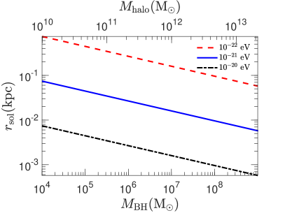
Figure 1: The soliton core radius with respect to the SMBH mass and the FDM halo mass for three different axion masses. Our analysis is valid in the region $r\gtrsim r_{\rm sol}$.

Cosmological simulations of FDM suggest that FDM haloes contain a solitonic central core whose density profile is empirically fit by the formula (Schive et al., 2014a)

$$\rho_{\text{core}}=\frac{\rho_{\rm sol}}{\left[1+0.091~{}\left(r/r_{\rm sol}\right)^{2}\right]^{8}},$$ (3)

where the soliton core radius can be expressed as

$$r_{\rm sol}=0.16{\rm kpc}\left(\frac{m}{10^{-22}{\rm eV}}\right)^{-1}\left(\frac{M_{H}}{10^{12}{\rm M_{\odot}}}\right)^{-1/3},$$ (4)

and $M_{H}$ is the halo, virial, mass. The characteristic soliton density is

$$\rho_{\rm sol}=2.94\times 10^{10}\left(\frac{m}{10^{-22}{\rm eV}}\right)^{-2}\left(\frac{r_{\rm sol}}{0.16{\rm kpc}}\right)^{-4}\frac{\rm M_{\odot}}{\rm kpc^{3}}$$ (5)

We will consider that a SMBH, associated with the FDM halo, is on an orbit that initially takes it well outside the soliton core, where the calculations of El-Zant et al. (2020) are strictly valid. Therefore, our analysis applies for $r\gtrsim r_{\rm sol}$, as in Figure 1. The SMBH may, in this context, be assumed to have been perturbed from the centre at some stage during the hierarchical galaxy formation scenario (e.g, during a major merger). In the case of a CDM halo it then spirals in by dynamical friction towards the very centre. In contrast, in the FDM scenario we consider here, the interplay and competition between fluctuations and dissipation results in the SMBH distance from the centre statistically satisfying energy equipartition (12). One main purpose here will be to investigate the stalling of SMBH mergers that accompany galactic mergers. In the context of this scenario, it will not be of crucial importance to model the density distribution precisely inside $r_{\rm sol}$. We assume that most FDM bound to the merging SMBH has been stripped and is dynamically unimportant, though we briefly discuss (in Section 4) the role of nuclear stellar clusters, surrounding SMBHs, in accellerating their final merger.

2.3 FDM halo

The profile given by (3) is not accurate outside the soliton core. It has been suggested that there the density can be described instead by the NFW profile, which joins smoothly with the above form at about three soliton radii $r_{\rm sol}$ (e.g, Mocz et al., 2019). According to recent numerical simulations of  Veltmaat et al. (2018), however, 6

6

in this region the velocities are well fitted by a Maxwellian distribution, suggesting that the density profile is nearly isothermal. Indeed, just outside the soliton core, the density profiles seems flatter than NFW. In this context, and in line with our assumption of Maxwellian distribution for velocity, we consider a profile that approximately fits a cored isothermal sphere, namely

$$\rho_{\text{halo}}=\frac{3\sigma_{H}^{2}}{2\pi Gr_{c}^{2}}g(x)\,,\text{where}\;g(x)=\frac{1+\frac{1}{3}x^{2}}{\left(1+x^{2}\right)^{2}}\,,\;x=\frac{r}{r_{c}}.$$ (6)

In Appendix A, we show that matching the core with the halo profiles at $3r_{\rm sol}$ gives

$$r_{c}=2~{}{\rm kpc}\left(\frac{m_{\rm axion}}{10^{-22}{\rm eV}}\right)^{-1}\left(\frac{M_{\rm B}}{10^{7}M_{\odot}}\right)^{-2/9},$$ (7)

where the scaling relations (1), (2) are assumed to hold.

The density profile (6) generates the logarithmic potential

$$\Phi=\sigma_{H}^{2}\ln\left(1+x^{2}\right),$$ (8)

and tends at large radii to that of a singular isothermal sphere with isotropic one-dimensional velocity dispersion $\sigma_{H}$. Nevertheless, the velocity dispersion varies as

$$\sigma_{\rm halo}=\sigma_{H}\,s(x)\,,\;\text{where}\;s(x)=\left(\frac{x^{2}+2}{x^{2}+3}\right)^{1/2},$$ (9)

as shown in Appendix B. For large $x$, this tends to unity; it differs by at most $18\%$ from this value at the very centre, validating our Maxwellian approximation for the velocity distribution.

3 Ejection of SMBHs

3.1 SMBH displacement

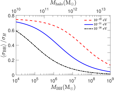
Figure 2: The average FDM-induced SMBH velocity dispersion $\left\langle\sigma_{\rm BH}\right\rangle$ scaled over the characteristic halo velocity dispersion $\sigma_{H}$ with respect to the SMBH and halo masses for different axion masses.

3.1.1 General considerations and scaling of SMBH velocity dispersion

We consider a black hole in the central region of an FDM sphere. The interfering de Broglie waves of the ultra light FDM axions lead to density fluctuations, which are related though the Poisson equation to potential fluctuations. Their dynamical effect on a classical particle can be described in a manner analogous to that of standard two body relaxation theory (Bar-Or et al., 2019; El-Zant et al., 2020). In this context, for a Maxwellian FDM velocity distribution, the FDM fluctuations are generated by granules of characteristic effective mass

$$m_{\rm eff}=\frac{\pi^{3/2}\hbar^{3}}{m_{\rm ax}{}^{3}\sigma^{3}}\rho,$$ (10)

where $m_{\rm ax}$ is the axion mass, $\rho$ is the average background density of FDM axions and $\sigma$ their one-dimensional velcoity dispersion. Adopting $\rho=\rho_{\rm halo}$ given in (6) and $\sigma=\sigma_{\rm halo}$ given in (9) we get

$$m_{\rm eff}=1.1\cdot 10^{7}M_{\odot}\left(\frac{m_{\rm ax}}{10^{-22}{\rm eV}}\right)^{-1}\left(\frac{M_{B}}{10^{7}M_{\odot}}\right)^{2/9}\frac{g(x)}{s(x)^{3}}.$$ (11)

As detailed in Appendix D, we stress that this is an effective description; the ’granules’ thus described are not long-lived classical particles. They arise instead from a formal equivalence with fluctuations giving rise to standard two body relaxation. The FDM power spectrum of fluctuations that gives rise to this description fully matches that inferred from numerical simulations. The effective ’size’ (and hence mass) of the quasiparticles in fact corresponds to a cutoff at the characteristic de Broglie wavelength in that spectrum, which has white noise structure on large scales.

We assume that the SMBH achieves equilibrium with the fluctuations; that is, there is a balance between the effects of fluctuation and dissipation, the latter being due to dynamical friction (for this to be the case the relevant relaxation time must be small enough, as discussed in Section 3.2). Because of equipartition, the velocity dispersion $\sigma_{B}$ of the SMBH is related to the FDM velocity dispersion as

$$M_{B}\sigma^{2}_{B}=m_{\rm eff}\sigma^{2}_{\rm eff}=\frac{1}{2}m_{\rm eff}\sigma_{\rm halo}^{2},$$ (12)

where $\sigma^{2}_{\rm eff}=\sigma_{\rm halo}^{2}/2$ refers to the effective velocity dispersion of the FDM quasiparticles with mass $m_{\rm eff}$ (cf. El-Zant et al. 2020). Substituting the effective mass from (10) we get the SMBH velocity dispersion

$$\sigma_{B}=73.8~{}\frac{\rm km}{\rm s}\left(\frac{m_{\rm ax}}{10^{-22}{\rm eV}}\right)^{-\frac{1}{2}}\left(\frac{M_{B}}{10^{7}M_{\odot}}\right)^{-1/6}\frac{g(x)^{1/2}}{s(x)^{1/2}},$$ (13)

and

$$\frac{\sigma_{B}}{\sigma_{\rm halo}}=0.74\left(\frac{m_{\rm ax}}{10^{-22}{\rm eV}}\right)^{-\frac{1}{2}}\left(\frac{M_{B}}{10^{7}M_{\odot}}\right)^{-7/18}\frac{g(x)^{1/2}}{s(x)^{3/2}}.$$ (14)

This scaling with mass is a result of the empirical relation (1), which implies a smaller SMBH mass relative to halo mass, combined with the fact that the de Broglie wavelengths (and effective masses) are larger for smaller haloes.

3.1.2 Expected RMS displacement from thermal average

The FDM halo acts as a heat bath for the SMBH, which will therefore undergo Brownian motion induced by the FDM fluctuations, with a characteristic radius reflecting a balance between the effect of fluctuations and that of the accompanying dissipation from dynamical friction. It has been shown by van Kampen (1988) that the one-particle probability distribution function of Brownian motion in inhomogeneous medium (presence of temperature gradient and external potential) is given at equilibrium by (see also Ryter 1981; Widder & Titulaer 1989; Nicolis 1965; Zubarev & Bashkirov 1968; Pérez-Madrid et al. 1994)

$$f(x)=\frac{\beta_{B}(x)\exp\left\{-\int_{0}^{x}d\tilde{x}\beta_{B}(\tilde{x})M_{\rm B}\Phi(\tilde{x})^{\prime}d\tilde{x}\right\}}{\int_{0}^{\infty}\beta_{B}(x)\exp\left\{-\int_{0}^{x}d\tilde{x}\beta_{B}(\tilde{x})M_{\rm B}\Phi(\tilde{x})^{\prime}d\tilde{x}\right\}4\pi x^{2}dx}$$ (15)

where a prime denotes a derivative and $\Phi(x)$ is given in (8). For the derivation and application in self-gravitating systems see Roupas (2020). We denote

$$\beta_{B}^{-1}\equiv m_{\rm eff}\sigma_{\rm eff}^{2}=M_{\rm B}\sigma_{\rm B}^{2}.$$ (16)

The probability (15) is the generalization of the Boltzmann propability $f_{B}\propto e^{-\beta m\Phi}$ in the case of varying $\beta$ and is the stationary solution of an appropriate Fokker-Planck equation given by van Kampen (1988). We may therefore average over $x$ any physical quantity $A(x)$ referring to the SMBH as

$$\left\langle A(x)\right\rangle=\int_{0}^{\infty}A(x)f(x)4\pi x^{2}dx.$$ (17)

The average SMBH velocity dispersion, scaled over the characteristic halo velocity dispersion $\sigma_{H}$, is plotted in Figure 2. It is higher for lighter axions and lighter SMBHs.

A statistical measure of the distance at which the SMBH may be ejected from the center is the RMS displacement, which is plotted in Figure 3. The displacement is numerically fit by the expression

$$r_{\rm RMS}\equiv\sqrt{\left\langle r^{2}\right\rangle}=1.84~{}{\rm kpc}\left(\frac{m_{\rm ax}}{10^{-22}{\rm eV}}\right)^{-\frac{3}{2}}\left(\frac{M_{B}}{10^{7}M_{\odot}}\right)^{-\frac{3}{5}}.$$ (18)

Evidently, it is higher for lighter SMBHs and lighter axions. This effect can explain observations indicating a dearth of SMBHs in the centers of dwarf galaxies. We discuss this further in Section 4. In addition, we infer that the displacement of the SMBH can be so large that it is completely ejected out of the bulge. Observations of SMBHs residing deep in their host bulges allow us constrain the axion mass. Requiring $r_{\rm RMS}\lesssim 0.1{\rm kpc}$ for Sagittarius $A^{*}$, with $M_{B}=4.1\cdot 10^{6}M_{\odot}$, constraints the axion mass to $m_{\rm ax}\gtrsim 10^{-21}{\rm eV}.$ Requiring that the RMS displacement from the centre be less than $1{\rm kpc}$, on the other hand, leads to the constraint $m_{\rm ax}\gtrsim 2\cdot 10^{-22}{\rm eV}$. Finally, we have $r_{\rm RMS}>0.1{\rm kpc}$ for all SMBHs lighter than $10^{9}M_{\odot}$, and for axions lighter than $10^{-22}{\rm eV}$.

3.1.3 Virial Theorem

We analyze further and validate the results regarding the RMS displacement (18), calculated as the average over the random walk (15) and displayed in Figure 3, by invoking the virial theorem for the SMBH. For the potential (8) the virial theorem translates to

$$\langle\ln(1+x^{2})\rangle=\left<3\frac{\sigma_{B}^{2}}{\sigma_{\rm halo}^{2}}\right>.$$ (19)

Using this equation we may estimate the RMS displacement without any need to assume a particular probability distribution in order to obtain the average.

This may be achieved as follows. For $x\la 1$, it is $\left\langle\ln(1+x^{2})\right\rangle\approx\langle x^{2}\rangle$. In this case, using (14) and (29) one may estimate the RMS displacement straightforwardly

$$\sqrt{\left\langle r^{2}\right\rangle}\approx 2.6~{}{\rm kpc}\left(\frac{m_{\rm ax}}{10^{-22}{\rm eV}}\right)^{-\frac{3}{2}}\left(\frac{M_{B}}{10^{7}M_{\odot}}\right)^{-\frac{11}{18}}\left<\frac{g(x)}{s(x)^{3}}\right>^{\frac{1}{2}}.$$ (20)

From (6) and (9), one deduces that $\frac{g(x)}{s(x)^{3}}$ is order one for $x\la 1$. Despite that the approximation is rough, the agreement with Eq. (18) is striking. The powers of masses are nearly identical, while even the scaling factor is matching very well. This self-consistency check provides further supporting evidence for the validity of our approach.

The condition $x\la 1$, combined with (19) implies that $\frac{3\sigma_{B}^{2}}{\sigma_{\rm halo}^{2}}\la 1$. Recalling again that $\frac{g(x)}{s(x)^{3}}$ is order one for $x\la 1$, from (14) this condition is seen to correspond to SMBH masses $\ga 10^{7}M_{\odot}$, when the axion mass is $10^{-22}{\rm eV}$. This in turn relates to halo masses $\ga 10^{12}M_{\odot}$. That is, the condition $x\la 1$ applies, in this case, to Milky Way-type haloes and above. For larger larger axion masses, the approximation holds for smaller halo and SMBH masses; in general, it is valid for $M_{B}\ga 10^{7}(\frac{m_{\rm ax}}{10^{-22}{\rm eV}})^{-9/7}M_{\odot}$.

For smaller masses the RMS displacements keep on increasing, even though $x$ can be larger than unity. To get an estimate of the expected excursion in this case, consider again equation (19), with $x\gg 1$. Now $\ln(1+x^{2})\rightarrow 2\ln x$ and $\langle 3\frac{g(x)}{s(x)^{3}}\rangle^{1/2}\rightarrow\langle x^{-2}\rangle^{1/2}\geq\langle x^{2}\rangle^{-1/2}$. In this case,

$$\sqrt{\langle r^{2}\rangle}\ga\frac{2.56~{}{\rm kpc}}{\sqrt{6\langle\ln x\rangle}}\left(\frac{m_{\rm ax}}{10^{-22}{\rm eV}}\right)^{-3/2}\left(\frac{M_{B}}{10^{7}M_{\odot}}\right)^{-11/18}.$$ (21)

Except for the weak root-logarithm dependence, this has the same scaling as in (20). The slightly weaker scaling is again consistent with the trend in figure 3.

Note finally that for small SMBH masses and $m_{\rm ax}<10^{-21}{\rm eV}$ the RMS displacement may be exceptionally large, even larger than the expected virial radius. Such displacement is therefore unrealistic. This is evident from Figure 3 and equation (35). We will see in Section 3.2 below, however, that the displacements from the centre are limited by the large relaxation time required to maintain thermal coupling between the SMBH and the FDM heat bath at low densities, characteristic of the outer halo.

3.1.4 Reduction of RMS radius by baryons

The RMS radius just evaluated reflects a statistical balance between fluctuations and dissipation. When the FDM mass fraction is decreased, as a baryonic component is introduced, the effect of fluctuations is suppressed relative to that of the dissipation. This leads to a smaller RMS radius at equilibrium, as we now estimate, focusing on the case of massive galaxies where the role of baryons is more prominent than in dark matter dominated dwarfs.

The energy dissipation rate, due to a dynamical friction force ${\bf F}_{D}$ acting on a particle moving with velocity ${\bf v}$, is ${\bf F}_{D}.{\bf v}$. For a particle of mass $m$, moving through field particles with masses $m_{a}$ and (strictly speaking homogeneous) density $\rho$, $F_{D}/m$ scales with these variables as $(m_{a}+m)\rho$ (e.g. Binney & Tremaine, 2008). Therefore, if an FDM halo hosts a system of stars of mass $m_{*}$, distributed with density $\rho_{*}$, the specific energy dissipation rate of an SMBH scales as $(m_{\rm eff}+M_{B})\rho_{\rm halo}+(m_{*}+M_{B})\rho_{*}$ (if the FDM is treated as a system of particles of mass $m_{\rm eff}$). From equation (11) one sees that $m_{\rm eff}\gg m_{*}$; and that for massive galaxies (with $M_{B}\ga 10^{7}M_{\odot}$), $M_{B}\ga m_{\rm eff}$ for $m_{\rm ax}\geq 10^{-22}{\rm eV}$. Thus the dissipation rate scales approximately as $\sim M_{B}(\rho_{\rm halo}+\rho_{*})=M_{B}~{}\rho$. It is therefore largely unchanged by the introduction of a stellar component, while keeping the total density constant. (Dynamical friction with a gaseous, rather than stellar, component would also contribute in approximately in the same manner; Ostriker, 1999).

The rate of energy gain due to fluctuations is quantified through the change of velocity variance $\left\langle(\Delta v)^{2}\right\rangle$ (cf. equation 22 below for the case of FDM). This does change when baryons are added. It scales as $m_{\rm eff}\rho_{\rm halo}+m_{*}\rho_{*}$. And as $m_{\rm eff}\gg m_{*}$, the baryons don’t contribute significantly to the fluctuations. The ratio of the energy gain, due to fluctuation, to energy loss, due to dissipation, then scales as $m_{\rm eff}/M_{B}\times\rho_{\rm halo}/\rho$; it decreases as the baryonic component is introduced, because $\rho_{\rm halo}/\rho$ is reduced, The reduction is equivalent to that obtained by keeping $\rho_{\rm halo}/\rho=1$ and decreasing $m_{\rm eff}/M_{B}$.

The equilibrium radius is in turn reduced. For, as the baryons do not participate in the fluctuations, the equilibrium condition (12) is modified to $M_{B}\sigma_{B}^{2}=\frac{1}{2}\frac{\rho_{\rm halo}}{\rho}m_{\rm eff}\sigma_{\rm halo}^{2}$. To estimate the effect for massive galaxies one can use (19), with $x\la 1$ as in Section 3.1.3 above. This gives $r_{\rm RMS}/r_{c}\approx\sqrt{3}\sigma_{B}/\sigma_{\rm halo}\approx\sqrt{m_{\rm eff}/M_{B}\times{\rho_{\rm halo}}/{\rho}}$. The equilibrium radius thus decreases with FDM fraction as $r_{\rm RMS}\sim(\rho_{\rm halo}/\rho)^{1/2}$. In addition, if the total density is kept constant, $m_{\rm eff}\propto\rho_{\rm halo}$ also decreases by a factor $\rho_{\rm halo}/\rho$ when baryons are added. The combined effect results in $r_{\rm RMS}\sim\rho_{\rm halo}/\rho$.

Since (from 10) $m_{\rm eff}$ also scales as $1/m_{\rm ax}^{3}$, the constraints on the axion mass are weakened by a factor $\sim(\rho_{\rm halo}/\rho)^{2/3}$. This is not very large, unless $\rho_{*}\gg\rho_{\rm halo}$. We will see in section 3.3, however, that out-of-equilibrium effects can still cause SMBHs interacting with baryons to inspiral towards the centre.

3.2 Relaxation time-scale

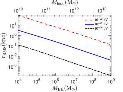
Figure 3: The RMS displacement $\sqrt{\left\langle r^{2}\right\rangle}$ of the SMBH random walk induced by FDM halo fluctuations.

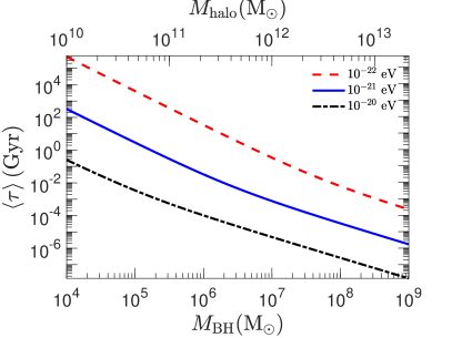
Figure 4: The average relaxation time of the SMBH-FDM halo system.

We calculate the relaxation time of the SMBH-FDM halo system as follows. When fluctuations are dominant over dissipation (dynamical friction) the velocity dispersion of the black hole is expected to increase with time as (see equation (62) in El-Zant et al. 2020)

$$\left\langle(\Delta v_{B})^{2}\right\rangle=t\frac{8\pi G^{2}\rho_{\rm halo}m_{\rm eff}\ln\Lambda}{\sigma_{\rm halo}}\,\frac{{\rm erf}(X)}{X},\quad X=\frac{v_{B}}{\sigma_{\rm halo}},$$ (22)

where $\ln\Lambda$ is the Coulomb logarithm (see Appendix C). The relaxation timescale of the black hole-dark matter halo system may be calculated by estimating the time it is required for $\Delta v_{B}\sim v_{B}$, when $v_{B}=\sigma_{B}\sqrt{3}$. Requiring in particular $\left\langle(\Delta v_{B})^{2}\right\rangle=3\sigma_{B}^{2}$ equation (22) then gives

$$\tau =\frac{3\sqrt{3}}{8\pi G^{2}\ln\Lambda}\frac{\sigma_{B}^{3}}{\rho_{\rm halo}m_{\rm eff}}\left\{{\rm erf}\left(X\right)\right\}^{-1}$$

$$=\frac{1.5}{\ln\Lambda}~{}{\rm Gyr}\left(\frac{m_{\rm ax}}{10^{-22}{\rm eV}}\right)^{-5/2}\left(\frac{M_{B}}{10^{7}M_{\odot}}\right)^{-29/18}$$

$$~{}\times\frac{s(x)^{3/2}}{g(x)^{1/2}{\rm erf}\left(X\right)}$$ (23)

where $X\equiv\frac{\sigma_{B}}{\sigma_{\rm halo}}\sqrt{3}$, and where we have used (13). Using (17) one can evaluate the average relaxation time $\left\langle\tau\right\rangle$. This is shown in Figure 4 where $\Lambda$ is given by Eq. (36). It is higher for lighter axion masses and lighter SMBHs. The relaxation time-scale is smaller than a Hubble time for all $m_{\rm ax}\geq 3\cdot 10^{-21}{\rm eV}$ and $M_{\rm BH}\geq 10^{4}M_{\odot}$. For $m_{\rm ax}=10^{-21}{\rm eV}$ and $m_{\rm ax}=10^{-22}{\rm eV}$ the time-scale is less than a Hubble time for $M_{\rm BH}\geq 5\cdot 10^{4}M_{\odot}$ and $M_{\rm BH}\geq 2\cdot 10^{6}M_{\odot}$, respectively. Self-consistency of our analysis, namely the use of equipartition conditions (12) and averages given by (17), requires that this be the case. Therefore the Sagittarius $A^{*}$ and heavier SMBHs are well probed by our analysis for axion masses $\gtrsim 10^{-22}{\rm eV}$. The SMBHs of dwarfs are probed by our analysis for axion masses as low as $\sim 10^{-21}{\rm eV}$.

3.3 LISA event reduction

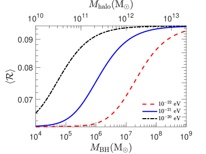
Figure 5: Estimated average event reduction rate of LISA for stellar to FDM density ratio of 0.2.

In the presence of the FDM halo, we have calculated that each SMBH will experience a random walk that will tend to keep them separated. At statistical equilibrium, the RMS displacement is given by Eq (18) and is displayed in Figure 3. The emergence of a stalling radius for SMBH mergers inside FDM haloes has been suggested already in (Hui et al., 2017; Bar-Or et al., 2019) in a different context. The stalling radius we propose here, $r_{\rm RMS}=\sqrt{\left\langle r^{2}\right\rangle}$, is statistical, as it is evaluated over the random walk Eq. (15), which is a stationary solution of a Fokker-Planck equation (van Kampen, 1988). This stalling radius is not strict but may be crossed randomly if a random kick is sufficiently intense.

If baryons are added to mass distribution, statistical equilibrium between fluctuation and dissipation, is perturbed. The fluctuations are unchanged but the magnitude of the dissipation (dynamical friction) is increased, and the stalling radius decreases (Section 3.1.4).

Departures from equilibrium may also lead to the inspiral of SMBH to the centre; and in merging systems bring a pair of SMBHs within range their combined sphere of influence, thus forming a binary (this is discussed further in Section 4). So the possibility of merger in an FDM scenario still exists. But the event rate of SMBH mergers observable by LISA should be significantly reduced.

The FDM equipartition timescale can be a good probe of the frequency and strength of the random fluctuations acting on the SMBHs, thus characterizing the span for the restoration to equilibrium in the presence of perturbation. If, for example, a large increase in dynamical friction due to coupling with a stellar component takes place, the restoration to equilibrium (with new stalling radius) will depend on the ability of the fluctuations to timely restore the system to the new equilibrium. A situation where this could be crucial involves an SMBH entering the central halo region, with significant baryon density, during a merger.

A first estimate of the reduction factor of the LISA event rate may thus involve only the ratio of the FDM equipartition timescale over the stellar dynamical friction timescale. We estimate the dynamical friction timescale as $\tau_{\star}\approx\sigma_{B}/|a_{\rm DF}|$, where $a_{\rm DF}$ denotes the dynamical friction deceleration caused by field stars. Substituting $a_{\rm DF}$ for a Maxwellian distribution as in (Binney & Tremaine, 2008) we get

$$\tau_{\star}=\frac{3\sqrt{3}}{4\pi G^{2}\ln\Lambda_{\star}}\frac{\sigma_{B}^{3}}{\rho_{\star}M_{\rm B}}\left\{{\rm erf}\left(X\right)-\frac{2X}{\sqrt{\pi}}e^{-X^{2}}\right\}^{-1},$$ (24)

where $\rho_{\star}$ is the stellar density. Dividing the equipartition timescale Eq. (23) over Eq. (24), we get

$$\frac{\tau}{\tau_{\star}}=\frac{1}{4}\frac{\ln\Lambda_{\star}}{\ln\Lambda}\frac{\sigma_{\rm halo}^{2}}{\sigma_{\rm B}^{2}}\frac{\rho_{\star}}{\rho_{\rm halo}}\left(1-\frac{2Xe^{-X^{2}}}{{\rm erf}(X)\sqrt{\pi}}\right)$$ (25)

We estimate the event reduction factor with the expression

$$\mathcal{R}\equiv 1-e^{-\frac{\tau}{\tau_{\star}}},$$ (26)

which is finite for all $\tau$, and converges to $\mathcal{R}\rightarrow\tau/\tau_{\star}$ for $\tau\ll\tau_{\star}$ and to $\mathcal{R}\rightarrow 1$ for $\tau\gg\tau_{\star}$. An average over the unperturbed equilibrium is implied.

In Figure 5 we plot the average event reduction factor $\left\langle\mathcal{R}\right\rangle$ with respect to SMBH mass for different axion masses, assuming $\rho_{\star}/\rho_{\rm halo}=0.2$ and $\ln\Lambda_{\star}\approx\ln\Lambda$. It is evident that for any axion mass and any SMBH mass. The event rate, thus deduced, is reduced by at least an order of magnitude, and is smaller for smaller systems.

4 Discussion

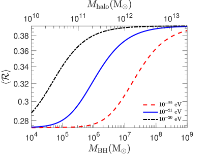
Figure 6: Same as in Figure 5, but for stellar to FDM density ratio of 1

SMBHs can be expelled from the centre of an FDM halo out to ${\rm kpc}$ scales for small halo-SMBH masses, as is clearly evident from Figure 3, even for $m_{\rm ax}=10^{-21}{\rm eV}$, which is consistent with most current constraints on FDM in dwarf galaxies. The effect being larger for smaller systems is a consequence of the fact that the ratio of SMBH to halo mass is smaller for smaller systems, the holes being lighter relative to the haloes at smaller masses. This combines with another effect; FDM fluctuations are larger in smaller systems, due to larger de Broglie wavelengths. (Equation 1).

This may have important consequences for observations of off-centre black holes in dwarf galaxies (Menezes et al., 2014, 2016; Reines et al., 2020; Shen et al., 2019). Explanations for this phenomenon usually involve dynamical dislocation as a result of a major merger, (e.g., Comerford & Greene, 2014; Bellovary et al., 2019), or ejection via large gravitational wave recoils (e.g, Komossa, 2012) during the final stages of such mergers. However major mergers of dwarfs are rare, especially at lower redshifts. A recent alternative invokes sinking of smaller substructures to the central parent halo region, dislocating the BH in the process (Boldrini et al. (2020)).

The present novel mechanism, involving FDM haloes, is different from the aforementioned attempts at explanation, as it involves a fundamental property of FDM. It also naturally explains why dislocated SMBH should be more common in small galaxies, for two crucial reasons: in addition to the aforementioned SMBH-Halo mass scaling relation favouring a large effect in smaller systems, the present mechanism is more efficient in dark matter-dominated galaxies, as we now discuss.

Conclusions regarding SMBH expulsion from the central regions of dark matter-dominated dwarfs are hardly affected if a modest baryonic component is added. Indeed, as we have seen, assuming a baryon fraction $\sim 0.2$ has little effect. The situation is however different if baryons dominate the mass distribution; in this case dynamical friction coupling with the SMBH can lead the latter to sink to the centre, the FDM fluctuations notwithstanding. In Section 3.1.4 we estimated that limits on the axion mass are decreased by a factor $(\rho_{\rm halo}/\rho)^{2/3}$, when a baryonic component of density $\rho_{*}=\rho-\rho_{\rm halo}$ is introduced while maintaining the equilibrium, thus decreasing the equilibrium RMS radius by a factor $\rho_{\rm halo}/\rho$. Such modifications are not very large, unless $\rho_{*}\gg rho_{\rm halo}$. However the out of equilibrium inspiraling, discussed in previous section is significantly enhanced already for $\rho_{*}$ of order $\rho_{\rm halo}$; as figure 6 suggests, the merger rate is much less efficiently suppressed in this case.

In Section 3 we derived the limit $m_{\rm ax}\ga 10^{-21}{\rm eV}$, by requiring the RMS displacement of the SMBH from the centre of the halo to be kept above $100{\rm pc}$ in massive systems. Observations reveal SMBHs at much smaller distances from the centre than $100{\rm pc}$. The significance of the $100{\rm pc}$ scale also comes from the fact that it is about an order of magnitude larger than the combined sphere of influence of SMBHs of the relevant masses. Current simulations show that, starting at separations a few times larger than the latter scale, a combination of few-body scattering and overlap of the nuclear clusters surrounding the black holes result in markedly accelerated decrease in separation, leading to a bound binary system (Khan et al., 2016, 2018; Ogiya et al., 2020). In this context, it becomes apparent that if one keeps the separation above $100{\rm pc}$, hierarchical SMBH growth can be effectively halted by FDM fluctuations when $m_{\rm ax}\ga 10^{-21}{\rm eV}$, if the effect of baryons is small. If a baryonic bulge component completely dominates the central dynamics, on the other hand, the weaker constraint $m_{\rm ax}\ga 10^{-22}{\rm eV}$, associated with few ${\rm kpc}$ scale RMS displacements, may be relevant. At smaller radii, dynamical friction coupling with the bulge stars can still cause the SMBH to sink. We now briefly discuss the robustness of this weaker constraint.

The decomposition of disk galaxies into bulge, disk and halo components is complex, and can lead to radically different results depending on assumptions, particularly regarding the mass-to-light ratios (e.g., Sofue, 2016; Richards et al., 2018). It is however unlikely that a three-dimensional baryonic component dominates most disk galaxies at scales larger than $\sim{\rm kpc}$. SMBHs of masses $10^{6}M_{\odot}\la M_{B}\la 10^{7}M_{\odot}$ are also observed in low surface brightness galaxies (Subramanian et al., 2016). Furthermore, in the FDM scenario, the same fluctuations leading to SMBH Brownian motions may also dilute the central density of the stellar component, inducing a core (Mocz et al., 2019). An axion mass of order $10^{-22}{\rm eV}$ should therefore be firmly ruled out.

In general, notwithstanding possible eventual baryon domination in the central region, SMBH growth may be severely impeded in FDM cosmologies at higher redshifts, as baryons are still settling into the halo potential wells. The impedance is likely to be far more efficient than in interacting dark matter models, where the formation of halo cores is sufficient to impede SMBH growth at higher $z$ (Cruz et al., 2020). As we show below, even with significant contributions from the baryons, the SMBH merging process may be dramatically slowed down in FDM haloes.

In addition to the role of baryons, another potential uncertainty involves soliton core dynamics. As already noted, our model in not strictly valid inside the soliton core. Core oscillations exist, and they can in principle contribute to the stochastic dynamics (Veltmaat et al. (2018); Marsh & Niemeyer (2018)), They are however likely to have different characteristics than those assumed here (see El-Zant et al., 2020 for discussion). Nevertheless, for the parameters of interest, equations (20) and (4) show that the ratio $r_{\rm sol}/r_{\rm RMS}\ll 1$; for example, at $M_{B}=10^{7}M_{\odot}$, this is about $1/16$ and $1/5$, for $m_{\rm ax}=10^{-22}{\rm eV}$ and $m_{\rm ax}=10^{-21}{\rm eV}$ respectively (and varies very weakly with SMBH mass). The volume enclosed by the soliton core relative to that comprised by the expected RMS radius is therefore of order a few times $10^{-4}$ to $10^{-2}$. Furthermore, as long as the relaxation time is longer than the crossing time, the motion is to a first approximation ballistic over such a timescale; an SMBH wandering into the core is therefore likely to enter not as a result of a diffusive process, involving small energy decrements, but with enough energy to exit the core on a crossing time rather than be trapped (the situation whereby motion affected by fluctuations remains approximately ballistic on a dynamical timescale is akin to described by the orbit averaged Fokker-Planck equation (Binney & Tremaine, 2008)). Finally, for a range of the relevant parameter space considered here the SMBH may in fact grow to swallow and subsume the central soliton within a Hubble time, in which case our calculations would be valid throughout the central halo (according to equations 59-60 of Hui et al., 2017, this should be the case for larger axion and halo masses).

Our calculations therefore suggest that an SMBH, dislocated well outside the core during a merger, may maintain a large RMS displacement, provided the FDM fluctuations are large enough to overcome any dynamical friction coupling with baryons. Given the halo density profile and the SMBH mass-halo mass empirical scaling relation, the strength of the fluctuations depends only on the axion mass. In terms of astrophysical consequences, the baryon distribution is therefore a more crucial issue than the question of proper theoretical modelling of core oscillations.

5 Conclusion

We have considered a central supermassive black hole immersed in a fuzzy dark matter halo of ultra-light axions. We argue that the SMBH will undergo Brownian motion induced by the FDM fluctuations due to the large de Broglie wavelength of axions. In effect, the FDM halo acts as a heat bath that expels the SMBH from the center of the halo. Our analysis applies outside the soliton core of FDM haloes. The physical picture therefore envisions a black hole that is initially displaced from the galaxy centres during a merger. We then examine whether its subsequent stochastic motion is characterized by a large RMS displacement.

The evaluation of RMS displacements assumes an SMBH in thermal equilibrium with the FDM heat bath. It thus presumes a small enough relaxation time, permitting equilibration. The relaxation timescale of the SMBH-FDM system is depicted in Figure 4. It is less than a Hubble time for both Sagittarius $A^{*}$ and heavier SMBHs for all axion masses considered here. SMBHs in dwarfs are probed by our model for axion masses in the range $m_{\rm ax}\gtrsim 10^{-21}{\rm eV}$. FDM-induced SMBH ejections for such systems still occur for smaller axion masses, but the relaxation time-scales are larger than a Hubble time. In these cases, the mean RMS displacements calculated here, assuming equilibration of the SMBH-FDM system, are overestimates that predict excursions larger than the expected virial radii of the host haloes. Out-of-equilibrium analysis is required to probe such cases with relaxation time-scales larger than a Hubble time.

In general, SMBH displacement from the centre is found to be much larger for small galaxies (equation (18) and Figure 3). This is a consequence of the scaling relation between SMBH and halo mass, with the central black holes predicted to be relatively lighter for less massive haloes (1). This combines with the fact that FDM fluctuations are larger in smaller systems, due to larger de Broglie wavelengths. FDM expulsion of SMBHs could thus explain the low detection rate of AGN in dwarf galaxies (Lupi et al., 2020), as the accretion would be mostly suppressed for an off-set black hole. Such off-set black holes are not excluded by observations even at low redshift (e.g., Shen et al., 2019). For dark matter-dominated dwarf galaxies, this conclusion is relatively robust and involves a fundamental physical phenomenon: fluctuations associated with the large de Broglie wavelengths of ultralight axions. In luminous galaxies, the role of the baryon distribution becomes important.

Our analysis further suggests that a lower bound on axion masses can be placed by heavier SMBHs, like Sagittarius $A^{*}$. For the SMBH to be kept at $100{\rm pc}$ from the centre requires an axion mass $m_{\rm ax}=\ga 10^{-21}{\rm eV}$, while displacement of $1{\rm kpc}$ leads to $m_{\rm ax}\ga 2~{}10^{-22}{\rm eV}$. In addition to well-centered SMBHs being observed at smaller radii, the significance of the $100{\rm pc}$ scale pertains in particular to the effective stalling of mergers. Numerical simulations show that when the separation of SMBH pairs in merging systems becomes significantly smaller, a markedly accelerated approach takes place, leading to bound binaries as the radii of influence overlap (e.g., Khan et al., 2018). A boson mass guaranteeing such separation may effectively impede any SMBH growth in a hierarchical structure formation scenario, provided the dark matter is dominant in the central region.

The weaker constraint $m_{\rm ax}\ga 10^{-22}{\rm eV}$, deduced from an assumed RMS displacement of a few ${\rm kpc}$, on the other hand, corresponds to a situation whereby a bulge component dominates the dynamics below this scale. In such a case, dynamical coupling between SMBHs and the stellar distribution may still lead to an inspiraling SMBH inside the bulge (Section 4). This may have interesting consequences, in this novel context, for the well-probed correlation between bulge and SMBH mass.

In general, however, even for significant baryon mass fractions, SMBH-binaries formed in galaxy mergers will tend to be softer due to the FDM fluctuations. The merging of such binaries will be significantly impeded; the event rate reduction factor depicted in Figure 5 predicts that, for a universal baryon fraction, the LISA event rate of SMBH mergers will be reduced by at least an order of magnitude within FDM haloes. The impeding effects of SMBH mergers apply for the whole halo-SMBH and axion mass range, but are more pronounced for lower mass SMBHs and lighter axion masses.

The suppression of SMBH growth in FDM models is expected to be generally larger at higher redshifts, as the baryons are still settling into the potential wells of haloes. This effect may also be expected to be far stronger than that recently reported in the context of self-interacting dark matter cosmologies (Cruz et al., 2020). In this case, the suppression is simply a result of the formation of cored dark matter haloes, decreasing the dynamical friction coupling with the dark matter, especially at higher redshift. Whereas in the FDM scenario, the suppression would equilibrium corresponding to large displacements from the centre.

Further work on the dynamics of SMBH-FDM systems, and its astrophysical implications, could include models allowing for more precise quantification and parameter variation. This may require moving beyond the current simple nearly isothermal fit and quasi-particle approximation, appropriate for FDM systems with Maxwellian distributions. A more general formulation could involve numerical simulations or Monte Carlo models of the Brownian motions. More detailed dynamical modelling may incorporate core oscillations (e.g. Veltmaat et al. (2018)), to include the effect of fluctuations near and inside the soliton core, where the model of El-Zant et al. (2020) employed here is not strictly valid. From an astrophysical point of view, more ambitious extensions would include a detailed examination of the competition and interplay between baryon and FDM components in determining the dynamics of SMBH.

Appendix A Core radius

We wish to determine the value of the softening radius $r_{c}$ which matches the core and halo profiles at some distance $r_{\star}=\alpha r_{\text{sol}}$ for some predetermined $\alpha$. We get

$$r_{c}=r_{\text{sol}}\sqrt{\frac{1}{2}\frac{\rho_{\text{I}}}{\rho_{\text{S}}}\left(1-2\frac{\rho_{\text{S}}}{\rho_{\text{I}}}\alpha^{2}+\sqrt{1-\frac{8}{3}\frac{\rho_{\text{S}}}{\rho_{\text{I}}}\alpha^{2}}\right)}$$ (27)

where the two characteristic densities are

$$\rho_{\text{S}}=\rho_{\rm core}(\alpha r_{\text{sol}}),\quad\rho_{\text{I}}=\frac{3\sigma_{H}^{2}}{2\pi Gr_{\text{sol}}^{2}}.$$ (28)

The soliton profile (5) is valid approximately up to $3r_{\text{sol}}$ (Mocz et al., 2019) and therefore we set $\alpha=3$ for the matching with the isothermal fit(6). Assuming relations (2), (1) between BH mass, halo mass and velocity dispersion, the equation (27) is accurately fit for $\alpha=3$ by

$$r_{c}=2.03~{}{\rm kpc}\left(\frac{m_{\rm axion}}{10^{-22}{\rm eV}}\right)^{-1}\left(\frac{M_{\rm BH}}{10^{7}M_{\odot}}\right)^{-2/9},$$ (29)

shown in Figure 7.

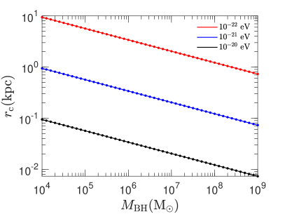
Figure 7: The characteristic halo radius $r_{c}$ with respect to the SMBH mass for three different axion masses. The dots correspond to the exact Eq. (27) and the solid line to the fit (29).

Appendix B Velocity dispersion profile

We wish to evaluate the vecloity dispersion profile associated with the density distribution (6) and potential (8). In general, for spherical systems with isotropic velocities the Jeans equation

$$\frac{d(\rho\sigma^{2})}{dr}=-\rho\frac{d\Phi}{dr}$$ (30)

applies. This has solution

$$\rho(r)\sigma^{2}(r)=-\int\rho(r)d\Phi+C.$$ (31)

For the density profile (6) $\rho(r)^{-1}\sim r^{2}$ at large radii, and therefore $C$ must be zero if the velocity dispersion is not to diverge at such radii. By evaluating the integral for the density and potential distributions given by  (6) and  (8) one then finds

$$\sigma(r)^{2}=\sigma_{H}^{2}\left[\frac{x^{2}+2}{x^{2}+3}\right],$$ (32)

The velocity dispersion thus tends to that of the singular isothermal sphere $\sigma_{H}$ at large radii and differs from this by at most a factor of $\sqrt{2/3}$ or about $18\%$.

The logarithmic derivative of the density distribution 6 is given by

$$\frac{d\ln\rho}{d\ln x}=-2~{}\frac{x^{4}+5x^{2}}{x^{4}+4x^{2}+3}.$$ (33)

Thus our density profile is flatter than the NFW cusp for radii $r\la 0.6r_{c}$ and has similar slope for larger radii of relevance to our calculations (up to a few $r_{c}$).

Appendix C Coulomb logarithm

We estimate the argument of the Coulomb logarithm entering equations (22) and (23). In the context of the stochastic model applied here, this is the ratio of maximal and minimal fluctuation scales of a Gaussian random field. It is thus given in terms of the maximal and minimal wavelength modes as $\Lambda=\lambda_{\rm max}/\lambda_{\rm min}$. Following Appendix E of El-Zant et al. (2020), we set the minimal scale to correspond to the size associated with the effective mass of the FDM granules: $m_{\rm eff}=\frac{4}{3}\rho_{\rm halo}\lambda_{\rm min}^{3}$. Using (10) gives

$$\lambda_{\rm min}=\left(\frac{3}{4}\right)^{1/3}\pi^{1/6}\frac{\hbar}{m_{\rm ax}\sigma_{\rm halo}}.$$ (34)

In El-Zant et al. (2020), the main concern was the effect of FDM fluctuations on disks. A cutoff was thus introduced to exclude longer wavelengths, as these would affect the disk nonlocally, possibly leading to the excitation of global modes, with consequences not captured by the stochastic model. In the present situation of an SMBH orbiting in the central region, all modes supported by the halo heat bath should contribute. We therefore set largest scales to correspond to the virial radius of the halo. For $\lambda$CDM cosmologies this may be approximated at redshift $z=0$ by (e.g., Appendix of Navarro et al., 1997)

$$\lambda_{\rm max}=R_{H}\approx 200~{}{\rm kpc}\left(\frac{M_{H}}{10^{12}M_{\odot}}\right)^{1/3}.$$ (35)

Using equation (34) in conjunction with (2), and neglecting the modest departures of $\sigma_{\rm halo}$ from $\sigma_{H}$ (cf. equation 9), one gets

$$\Lambda\approx 1000~{}\left(\frac{m_{\rm ax}}{10^{-22}}\right)\left(\frac{M_{H}}{10^{12}M_{\odot}}\right)^{2/3}.$$ (36)

Appendix D The advent of effective quasiparticle picture

The description of FDM fluctuations used here involved an effective mass, velocity dispersion and Coulomb logarithm. However it is important to point out that this effective picture does not require the fluctuations to behave as long lived classical particles. Indeed, the standard Chandrasekhar estimates of relaxation and dynamical friction are quite conveniently recovered by formulating the problem in Fourier space. In this way it is possible to describe classical two body relaxation in terms of a superposition of waves, even though, physically speaking, one is describing a medium of discrete particles ((El-Zant et al., 2020; Bar-Or et al., 2019). In the same generic manner one can also describe the effect of fluctuations arising from fully developed turbulence, even though one deals with a fluid (El-Zant et al., 2016).

In this context, El-Zant et al. (2020) applied the model initially developed for turbulent media to systems of classical particles and to interfering FDM waves. They thus found it possible to recover the results of classical two body relaxation, in addition to an analogous effect due to the interfering FDM de Broglie waves. The effective description of FDM fluctuations transpired by relating the results of the latter analysis to those of classical two body relaxation. But the quasiparticles, that thus arise, are no more classical particles than the Fourier modes entering into the derivation of classical two body relaxation are ’real’ (physical) classical waves. As we now discuss, they simply correspond to a cutoff scale of a power spectrum of interfering waves, which in fact has a white noise form on larger scales.

D.1 Density fluctuations

We start with the density contrast power spectrum. Following El-Zant et al. (2020), this is given by

$$\mathcal{P}({\bf k},t)\!=\!\frac{(2\pi)^{3}}{\rho_{0}^{2}}\!\!\int\!\!d{\bf v_{1}}d{\bf v_{2}}f(\!{\bf v}_{1}\!)f(\!{\bf v}_{2}\!)\delta_{D}({\bf k}-m_{\hbar}\!{\bf v}_{d})e\!^{-im_{\hbar}({\bf v}_{c}.{\bf v}_{d})t},$$ (37)

where

$$m_{\hbar}=2m_{\rm ax}/\hbar,$$ (38)

${\bf v}_{i}=\hbar{\bf k}_{i}/m$ are de Broglie wave packet group velocities, and ${\bf v}_{c}$ and ${\bf v}_{d}$ correspond to the sum and differences of the phase velocities of interfering waves; such that $2{\bf v}_{c}={\bf v}_{1}+{\bf v}_{2}$, and $2{\bf v}_{d}={\bf v}_{1}-{\bf v}_{2}$. For a Maxwellian velocity distribution the equal time power spectrum was shown to agree nicely with power spectra inferred from numerical simulation; the spectra in both the theory and simulations simply correspond to a white noise power spectrum with cutoff scale characteristic of the typical de Broglie wavelength. Indeed, for a system with velocity dispersion $\sigma$, the RMS fluctuations on scale $R$ were found to decrease as

$$\sigma_{R}^{2}=\left(\frac{2}{(R\sigma m_{\hbar})^{2}+2}\right)^{3/2},$$ (39)

characteristic of white noise decline on scales $R\gg\sigma m_{\hbar}$. The density correlation functions (especially in the temporal regime) also agreed with published simulation results.

D.2 Dynamical effect in terms of quasiparticles

The quasiparticle picture arises from the aforementioned power spectrum cutoff as follows. The density fluctuations give rise to force fluctuations (through the Poisson equation). When assumed to form a random Gaussian field, these can be quantified through the force correlation function. El-Zant et al. (2020) find this to be given by

$$\langle{\bf F}(0,0).{\bf F}(r, t)\rangle=$$

$$\left(\frac{4\pi G}{m_{\hbar}}\right)^{2}\!\!\!\int\!\frac{e^{im_{\hbar}({\bf v}_{d}.{\bf r}-{\bf v}_{c}.{\bf v}_{d}t)}}{v_{d}^{2}}f({\bf v}_{1})f({\bf v}_{2})d{\bf v}_{1}d{\bf v}_{2}.$$ (40)

Assuming isotropy, the velocity dispersion arising from the fluctuations after time $T$, for a classical test particle moving with velocity ${\bf v}_{p}$ — $\langle(\Delta v_{p})^{2}\rangle=2\int_{0}^{T}(T-t)\langle{\bf F}(0).{\bf F}(t)\rangle dt$ — can then be written as

$$\langle(\Delta v_{p})^{2}\rangle=A\!\int\!\! (T-t)f({\bf v}_{c}+{\bf v}_{d})f({\bf v}_{c}-{\bf v}_{d})$$

$$\times\frac{\sin\left(m_{\hbar}v_{d}|{\bf v}_{p}-{\bf v}_{c}|t\right)}{m_{\hbar}v_{d}|{\bf v}_{p}-{\bf v}_{c}|t}~{}d{\bf v}_{c}dv_{d}dt,$$ (41)

where $A=2(8\pi)^{3}G^{2}m_{\hbar}^{-2}$.

In El-Zant et al. (2020) it is argued that, as the integral is dominated by the region $v_{d}\ll v_{c}$, both distribution functions figuring in this equation can be approximated as $f({\bf v}_{c})$. If this is the case, in the diffusion (large $T$) limit, one finds

$$\langle(\Delta v_{p})^{2}\rangle=\left(\frac{4\pi}{m_{\hbar}}\right)^{3}8\pi G^{2}T\ln\Lambda\int d{\bf v}_{c}\frac{f^{2}({\bf v}_{c})}{|{\bf v}_{p}-{\bf v}_{c}|},$$ (42)

where here

$$\Lambda=\frac{v_{dx}}{v_{dm}},$$ (43)

is a ratio of maximal and minimal speeds, which are proportional to corresponding wavenumbers by virtue of the de Broglie relation.

Introducing

$$m_{\rm eff}=\left(\frac{4\pi}{m_{\hbar}}\right)^{3}\frac{\int f^{2}({\bf v})d{\bf v}}{\int f({\bf v})d{\bf v}},$$ (44)

where $m_{\hbar}$ is given by (38) and

$$f_{\rm eff}({\bf v})=\frac{\int f({\bf v})d{\bf v}}{\int f^{2}({\bf v})d{\bf v}}f^{2}({\bf v}),$$ (45)

makes (42) formally equivalent to the expression describing the increase in velocity dispersion due to fluctuations arising from a distribution of classical field particles of mass $m$ (El-Zant et al., 2020; Binney & Tremaine, 2008 Appendix L)

$$\langle(\Delta v_{p})^{2}\rangle=8\pi mG^{2}T\ln\Lambda\int d{\bf v}\frac{f({\bf v})}{|{\bf v}_{p}-{\bf v}|}.$$ (46)

In the standard derivation $\Lambda$ corresponds to a ratio of maximal and minimal impact parameters, while when the fluctuating field is Fourier analysed it corresponds to a ratio of maximal and minimal cutoff wavelengths (or wavenumbers).

The approximation that leads to this formal equivalence between FDM and classical particle systems, effectively assumes a long wavelength limit in the power spectrum of fluctuations, which then simply corresponds to white noise. The small scale cutoff at the characteristic de Broglie wavelength is accounted for by the large velocity (small spatial scale) cutoff determined in the Coulomb logarithm (43). This approximation would be exact for a distribution function in the form of a step function, with sharp cutoff at the characteristic wavelength, corresponding to an effective ’size’ for the quasiparticles; for in this case the $1/v_{d}$ in equation (41) need not be integrated over the distribution functions. Its independent integration leads to the Coulomb logarithm,

In El-Zant et al. (2020), it is furthermore argued that this is also a good approximation for Maxwellians, which are roughly constant for smaller speeds, before quickly cutting off beyond a certain characteristic value (corresponding to larger wavenumbers and smaller spatial scales). We now show explicitly that this is indeed the case.

D.3 Validity for Maxwellian distributions

For the Maxwellian distribution

$$f(v)=\frac{\rho_{0}}{(2\pi\sigma^{2})^{3/2}}e^{-\frac{v^{2}}{2\sigma^{2}}},$$ (47)

equation (41) becomes

$$\langle(\Delta v_{p})^{2}\rangle=B~{}\!\int\!\! (T-t)e^{-\frac{1}{\sigma^{2}}[({\bf v}_{c}+{\bf v}_{d})^{2}+({\bf v}_{c}-{\bf v}_{d})^{2}]}$$

$$\times\frac{\sin\left(m_{\hbar}v_{d}|{\bf v}_{p}-{\bf v}_{c}|t\right)}{m_{\hbar}v_{d}|{\bf v}_{p}-{\bf v}_{c}|t}~{}d{\bf v}_{c}dv_{d}dt,$$ (48)

where $B=A~{}\rho_{0}^{2}/(2\pi\sigma^{2})^{3}$.

Expanding the squares in the exponential, then integrating over time and taking the diffusion limit ($T\gg m_{\hbar}v_{d}|{\bf v}_{p}-{\bf v}_{c}|$), this becomes

$$\langle(\Delta v_{p})^{2}\rangle=\left(\frac{4\pi}{m_{\hbar}}\right)^{3}8\pi G^{2}T\int\frac{e^{-\frac{v_{d}^{2}}{\sigma^{2}}}}{v_{d}}dv_{d}\int d{\bf v}_{c}\frac{f^{2}({\bf v}_{c})}{|{\bf v}_{p}-{\bf v}_{c}|}.$$ (49)

This is the same as equation (42) above, except that the Coulomb logarithm is replaced by integration of $1/v_{d}$ weighed by the exponential (this result was arrived at from a different procedure in Bar-Or et al., 2019).

To compare (49) with (42), we explicitly evaluate the integral of $1/v_{d}$. As the contribution from larger $v_{d}$ is now naturally cutoff by this weighing, we need not impose an artificial high speed (wavenumber) cutoff; thus we may set $v_{dx}\rightarrow\infty$. The minimal cutoff is still limited by the system size (as described in the previous Appendix). We can thus evaluate this integral as follows:

$$\int_{v_{dm}}^{\infty}\frac{e^{-\frac{v_{d}^{2}}{\sigma^{2}}}}{v_{d}}dv_{d}=-\frac{1}{2}{\rm Ei}\left(-\frac{v_{dm}^{2}}{\sigma^{2}}\right)\simeq\ln\left(\frac{\sigma}{v_{dm}}\right)-0.29,$$ (50)

where ${\rm Ei}$ is the exponetial integral, 0.29 stands for an approximation to half the Euler–Mascheroni constant, and where we ignore terms of order $(v_{dm}/\sigma)^{2}$ and higher; as from (34), $\sigma\simeq\sigma_{\rm halo}$ approximately corresponds to the minimal de Broglie scale, while $v_{dx}$ is associated with the much larger maximum scale (given by 35).

Setting

$$v_{dx}=\frac{\hbar}{m_{\rm ax}\lambda_{\rm max}},$$ (51)

with $\lambda_{\rm max}$ given by (35), gives a ratio

$$\frac{\int_{v_{dm}}^{\infty}e^{-\frac{v_{d}^{2}}{\sigma^{2}}}dv_{d}}{\ln\Lambda}=\frac{\ln\left(\frac{3}{4}\right)^{1/3}\pi^{1/6}\Lambda-0.29}{\ln\Lambda}=1-\frac{0.19}{\ln\Lambda}.$$ (52)

With $\Lambda$ given by (36), the second term in the last equality is small. Which means that the exact integral over the distribution function quite accurately corresponds in this case with the approximation in terms of Coulomb logarithm, from which the correspondence with classical relaxation, and the notions of effective mass and distribution function, arose.

Thus, for a Maxwellian distribution, the quasi-particle picture is accurate, with the exact results recovered via a judicious choice of the Coulomb logarithm, with a natural spatial cutoff scale corresponding to the characteristic ’size’ of effective quasiparticles. This cutoff is directly related to that in the power spectrum of density fluctuations, which matches well the results of numerical simulations.

References

- Amorisco & Loeb (2018) Amorisco N. C., Loeb A., 2018, arXiv e-prints, p. arXiv:1808.00464
- Arcadi et al. (2018) Arcadi G., Dutra M., Ghosh P., Lindner M., Mambrini Y., Pierre M., Profumo S., Queiroz F. S., 2018, European Physical Journal C, 78, 203
- Bandara et al. (2009) Bandara K., Crampton D., Simard L., 2009, ApJ, 704, 1135
- Bar-Or et al. (2019) Bar-Or B., Fouvry J.-B., Tremaine S., 2019, ApJ, 871, 28
- Bar et al. (2019) Bar N., Blum K., Lacroix T., Panci P., 2019, arXiv e-prints, p. arXiv:1905.11745
- Baumann et al. (2019) Baumann D., Chia H. S., Porto R. A., 2019, Physical Review D, 99
- Bellovary et al. (2019) Bellovary J. M., Cleary C. E., Munshi F., Tremmel M., Christensen C. R., Brooks A., Quinn T. R., 2019, MNRAS, 482, 2913
- Binney & Tremaine (2008) Binney J., Tremaine S., 2008, Galactic dynamics
- Bode et al. (2001) Bode P., Ostriker J. P., Turok N., 2001, ApJ, 556, 93
- Boldrini et al. (2020) Boldrini P., Mohayaee R., Silk J., 2020, MNRAS,
- Boveia & Doglioni (2018) Boveia A., Doglioni C., 2018, Annual Review of Nuclear and Particle Science, 68, annurev
- Brito et al. (2015) Brito R., Cardoso V., Pani P., 2015, Lecture Notes in Physics
- Bullock & Boylan-Kolchin (2017) Bullock J. S., Boylan-Kolchin M., 2017, Annual Review of Astronomy and Astrophysics, 55, 343
- Burkert (2000) Burkert A., 2000, ApJ, 534, L143
- Burkert (2020) Burkert A., 2020, arXiv e-prints, p. arXiv:2006.11111
- Church et al. (2018) Church B. V., Ostriker J. P., Mocz P., 2018, arXiv e-prints, p. arXiv:1809.04744
- Cole et al. (2011) Cole D. R., Dehnen W., Wilkinson M. I., 2011, MNRAS, 416, 1118
- Colín et al. (2000) Colín P., Avila-Reese V., Valenzuela O., 2000, ApJ, 542, 622
- Comerford & Greene (2014) Comerford J. M., Greene J. E., 2014, ApJ, 789, 112
- Cruz et al. (2020) Cruz A., et al., 2020, arXiv e-prints, p. arXiv:2004.08477
- Davies & Mocz (2019) Davies E. Y., Mocz P., 2019, arXiv:1908.04790,
- Davis et al. (2019) Davis B. L., Graham A. W., Combes F., 2019, ApJ, 877, 64
- Davoudiasl & Denton (2019) Davoudiasl H., Denton P. B., 2019, arXiv e-prints, p. arXiv:1904.09242
- Del Popolo & Le Delliou (2017) Del Popolo A., Le Delliou M., 2017, Galaxies, 5, 17
- Del Popolo et al. (2014) Del Popolo A., Lima J. A. S., Fabris J. C., Rodrigues D. C., 2014, J. Cosmology Astropart. Phys., 4, 21
- Deng et al. (2018) Deng H., Hertzberg M. P., Namjoo M. H., Masoumi A., 2018, Phys. Rev. D, 98, 023513
- Desjacques & Nusser (2019) Desjacques V., Nusser A., 2019, arXiv e-prints, p. arXiv:1905.03450
- El-Zant et al. (2001) El-Zant A., Shlosman I., Hoffman Y., 2001, ApJ, 560, 636
- El-Zant et al. (2004) El-Zant A. A., Hoffman Y., Primack J., Combes F., Shlosman I., 2004, ApJ, 607, L75
- El-Zant et al. (2015) El-Zant A., Khalil S., Sil A., 2015, Phys. Rev. D, 91, 035030
- El-Zant et al. (2016) El-Zant A. A., Freundlich J., Combes F., 2016, MNRAS, 461, 1745
- El-Zant et al. (2020) El-Zant A. A., Freundlich J., Combes F., Halle A., 2020, MNRAS, 492, 877
- Elbert et al. (2015) Elbert O. D., Bullock J. S., Garrison-Kimmel S., Rocha M., Oñorbe J., Peter A. H. G., 2015, MNRAS, 453, 29
- Evrard et al. (2008) Evrard A. E., et al., 2008, ApJ, 672, 122
- Ferrarese (2002) Ferrarese L., 2002, ApJ, 578, 90
- Frenk & White (2012) Frenk C. S., White S. D. M., 2012, Annalen der Physik, 524, 507
- Freundlich et al. (2019) Freundlich J., Dekel A., Jiang F., Ishai G., Cornuault N., Lapiner S., Dutton A. A., Maccio A. V., 2019, arXiv e-prints, p. arXiv:1907.11726
- Goerdt et al. (2010) Goerdt T., Moore B., Read J. I., Stadel J., 2010, ApJ, 725, 1707
- Goodman (2000) Goodman J., 2000, New Astron., 5, 103
- Governato et al. (2012) Governato F., et al., 2012, MNRAS, 422, 1231
- Hayashi et al. (2020) Hayashi K., Chiba M., Ishiyama T., 2020, arXiv e-prints, p. arXiv:2007.13780
- Hu et al. (2000) Hu W., Barkana R., Gruzinov A., 2000, Physical Review Letters, 85, 1158
- Hui et al. (2017) Hui L., Ostriker J. P., Tremaine S., Witten E., 2017, Phys. Rev. D, 95, 043541
- Khan et al. (2016) Khan F. M., Fiacconi D., Mayer L., Berczik P., Just A., 2016, ApJ, 828, 73
- Khan et al. (2018) Khan F. M., Capelo P. R., Mayer L., Berczik P., 2018, ApJ, 868, 97
- Klypin et al. (2011) Klypin A. A., Trujillo-Gomez S., Primack J., 2011, ApJ, 740, 102
- Kobayashi et al. (2017) Kobayashi T., Murgia R., De Simone A., Iršič V., Viel M., 2017, Phys. Rev. D, 96, 123514
- Kochanek & White (2000) Kochanek C. S., White M., 2000, ApJ, 543, 514
- Komossa (2012) Komossa S., 2012, Advances in Astronomy, 2012, 364973
- Lazar et al. (2020) Lazar A., et al., 2020, MNRAS, 497, 2393
- Lidz & Hui (2018) Lidz A., Hui L., 2018, Phys. Rev. D, 98, 023011
- Lovell et al. (2014) Lovell M. R., Frenk C. S., Eke V. R., Jenkins A., Gao L., Theuns T., 2014, MNRAS, 439, 300
- Lupi et al. (2020) Lupi A., Sbarrato T., Carniani S., 2020, Monthly Notices of the Royal Astronomical Society, 492, 2528–2534
- Macciò et al. (2012) Macciò A. V., Paduroiu S., Anderhalden D., Schneider A., Moore B., 2012, MNRAS, 424, 1105
- Madau et al. (2014) Madau P., Shen S., Governato F., 2014, ApJ, 789, L17
- Marsh (2016) Marsh D. J. E., 2016, Phys. Rep., 643, 1
- Marsh (2017) Marsh D. J. E., 2017, arXiv e-prints, p. arXiv:1712.03018
- Marsh & Niemeyer (2018) Marsh D. J. E., Niemeyer J. C., 2018, arXiv e-prints, p. arXiv:1810.08543
- Marsh & Silk (2014) Marsh D. J. E., Silk J., 2014, MNRAS, 437, 2652
- Martizzi et al. (2013) Martizzi D., Teyssier R., Moore B., 2013, MNRAS, 432, 1947
- Mashchenko et al. (2006) Mashchenko S., Couchman H. M. P., Wadsley J., 2006, Nature, 442, 539
- Mashchenko et al. (2008) Mashchenko S., Wadsley J., Couchman H. M. P., 2008, Science, 319, 174
- Menezes et al. (2014) Menezes R. B., Steiner J. E., Ricci T. V., 2014, ApJ, 796, L13
- Menezes et al. (2016) Menezes R. B., Steiner J. E., da Silva P., 2016, ApJ, 817, 150
- Miralda-Escudé (2002) Miralda-Escudé J., 2002, ApJ, 564, 60
- Mocz et al. (2019) Mocz P., et al., 2019, Phys. Rev. Lett., 123, 141301
- Mutlu-Pakdil et al. (2018) Mutlu-Pakdil B., Seigar M. S., Hewitt I. B., Treuthardt P., Berrier J. C., Koval L. E., 2018, MNRAS, 474, 2594
- Nadler et al. (2020) Nadler E. O., et al., 2020, arXiv e-prints, p. arXiv:2008.00022
- Navarro et al. (1997) Navarro J. F., Frenk C. S., White S. D. M., 1997, ApJ, 490, 493
- Nebrin et al. (2018) Nebrin O., Ghara R., Mellema G., 2018, arXiv e-prints, p. arXiv:1812.09760
- Nicolis (1965) Nicolis G., 1965, J. Chem. Phys., 43, 1110
- Niemeyer (2019) Niemeyer J. C., 2019, arXiv e-prints, p. arXiv:1912.07064
- Nipoti & Binney (2015) Nipoti C., Binney J., 2015, MNRAS, 446, 1820
- Nori et al. (2019) Nori M., Murgia R., Iršič V., Baldi M., Viel M., 2019, MNRAS, 482, 3227
- Ogiya & Mori (2014) Ogiya G., Mori M., 2014, ApJ, 793, 46
- Ogiya et al. (2020) Ogiya G., Hahn O., Mingarelli C. M. F., Volonteri M., 2020, MNRAS, 493, 3676
- Ostriker (1999) Ostriker E. C., 1999, ApJ, 513, 252
- Peebles (2000) Peebles P. J. E., 2000, ApJ, 534, L127
- Peirani et al. (2008) Peirani S., Kay S., Silk J., 2008, A&A, 479, 123
- Pérez-Madrid et al. (1994) Pérez-Madrid A., Rubí J. M., Mazur P., 1994, Physica A Statistical Mechanics and its Applications, 212, 231
- Peter et al. (2013) Peter A. H. G., Rocha M., Bullock J. S., Kaplinghat M., 2013, MNRAS, 430, 105
- Pontzen & Governato (2012) Pontzen A., Governato F., 2012, MNRAS, 421, 3464
- Pontzen & Governato (2014) Pontzen A., Governato F., 2014, Nature, 506, 171
- Read & Gilmore (2005) Read J. I., Gilmore G., 2005, MNRAS, 356, 107
- Reines et al. (2020) Reines A. E., Condon J. J., Darling J., Greene J. E., 2020, ApJ, 888, 36
- Richards et al. (2018) Richards E. E., et al., 2018, Monthly Notices of the Royal Astronomical Society, 476, 5127
- Robles et al. (2019) Robles V. H., Bullock J. S., Boylan-Kolchin M., 2019, MNRAS, 483, 289
- Romano-Díaz et al. (2008) Romano-Díaz E., Shlosman I., Hoffman Y., Heller C., 2008, ApJ, 685, L105
- Roszkowski et al. (2018) Roszkowski L., Sessolo E. M., Trojanowski S., 2018, Reports on Progress in Physics, 81, 066201
- Roupas (2020) Roupas Z., 2020, arXiv e-prints, p. arXiv:2006.12755
- Ryter (1981) Ryter D., 1981, Zeitschrift fur Physik B Condensed Matter, 41, 39
- Safarzadeh & Spergel (2019) Safarzadeh M., Spergel D. N., 2019, arXiv e-prints, p. arXiv:1906.11848
- Schive et al. (2014a) Schive H.-Y., Chiueh T., Broadhurst T., 2014a, Nature Physics, 10, 496
- Schive et al. (2014b) Schive H.-Y., Liao M.-H., Woo T.-P., Wong S.-K., Chiueh T., Broadhurst T., Hwang W.-Y. P., 2014b, Physical Review Letters, 113, 261302
- Schneider et al. (2012) Schneider A., Smith R. E., Macciò A. V., Moore B., 2012, MNRAS, 424, 684
- Shao et al. (2013) Shao S., Gao L., Theuns T., Frenk C. S., 2013, MNRAS, 430, 2346
- Shen et al. (2019) Shen Y., Hwang H.-C., Zakamska N., Liu X., 2019, The Astrophysical Journal, 885, L4
- Silk (2017) Silk J., 2017, ApJ, 839, L13
- Sofue (2016) Sofue Y., 2016, PASJ, 68, 2
- Spergel & Steinhardt (2000) Spergel D. N., Steinhardt P. J., 2000, Physical Review Letters, 84, 3760
- Subramanian et al. (2016) Subramanian S., Ramya S., Das M., George K., Sivarani T., Prabhu T. P., 2016, MNRAS, 455, 3148
- Teyssier et al. (2013) Teyssier R., Pontzen A., Dubois Y., Read J. I., 2013, MNRAS, 429, 3068
- Tonini et al. (2006) Tonini C., Lapi A., Salucci P., 2006, ApJ, 649, 591
- Veltmaat et al. (2018) Veltmaat J., Niemeyer J. C., Schwabe B., 2018, Physical Review D, 98
- Widder & Titulaer (1989) Widder M. E., Titulaer U. M., 1989, Physica A Statistical Mechanics and its Applications, 154, 452
- Zavala et al. (2013) Zavala J., Vogelsberger M., Walker M. G., 2013, MNRAS, 431, L20
- Zolotov et al. (2012) Zolotov A., et al., 2012, ApJ, 761, 71
- Zubarev & Bashkirov (1968) Zubarev D. N., Bashkirov A. G., 1968, Physica, 39, 334
- van Kampen (1988) van Kampen N., 1988, Journal of Physics and Chemistry of Solids, 49, 673