Operator-valued formulas for Riemannian Gradient and Hessian and families of tractable metrics
Abstract.
We provide an explicit formula for the Levi-Civita connection and Riemannian Hessian for a Riemannian manifold that is a quotient of a manifold embedded in an inner product space with a non-constant metric function. Together with a classical formula for projection, this allows us to evaluate Riemannian gradient and Hessian for several families of metrics on classical manifolds, including a family of metrics on Stiefel manifolds connecting both the constant and canonical ambient metrics with closed-form geodesics. Using these formulas, we derive Riemannian optimization frameworks on quotients of Stiefel manifolds, including flag manifolds, and a new family of complete quotient metrics on the manifold of positive-semidefinite matrices of fixed rank, considered as a quotient of a product of Stiefel and positive-definite matrix manifold with affine-invariant metrics. The method is procedural, and in many instances, the Riemannian gradient and Hessian formulas could be derived by symbolic calculus. The method extends the list of potential metrics that could be used in manifold optimization and machine learning.
Key words and phrases:
Optimization, Riemannian Hessian, Stiefel,Positive-definite, Positive-semidefinite, Flag manifold, Machine Learning.1991 Mathematics Subject Classification:
65K10, 58C05, 49Q12, 53C25, 57Z20, 57Z25, 68T051. Introduction
In this article, we attempt to address the problem: given a manifold, described by constraint equations and a metric, also defined by an analytic formula, compute the Levi-Civita connection, Riemannian Hessian, and gradient for a function on the manifold. By computing, we mean a procedural, not necessarily closed-form approach. We are looking for a sequence of equations, operators, and expressions to solve and evaluate, rather than starting from a distance minimizing problem. We believe that the approach we take, using a classical formula for projections together with an adaptation of the Christoffel symbol calculation to ambient space addresses the problem effectively for many manifolds encountered in applications. This method provides a very explicit and transparent procedure that we hope will be helpful to researchers in the field. The main feature is it can handle manifolds with non-constant embedded metrics, such as Stiefel manifolds with the canonical metrics, or the manifold of positive-definite matrices with the affine-invariant metrics. The method allows us to compute Riemannian gradients and Hessian for several new families of metrics on manifolds often encountered in applications, including optimization and machine learning. While the effect of changing metrics on first-order optimization methods has been considered previously, we hope this will lead to future works on adapting metrics to second-order methods. The approach is also suitable in the case where the gradient formula is not of closed-form. We also provide a number of useful identities known in special cases.
As an application of the method developed here, we give a short derivation of the gradient and Hessian of a family of metrics studied recently in [11], extending both the canonical and embedded metric on the Stiefel manifolds with a closed-form geodesics formula. We derive the Riemannian framework for the induced metrics on quotients of Stiefel manifolds, including flag manifolds. We also give complete metrics on the fixed-rank positive-semidefinite matrix manifolds, with efficiently computable gradient, Hessian and geodesics.
1.1. Background
In the foundational paper [9], the authors computed the geodesic equation for a Stiefel manifold of matrices satisfying , with both the constant metric on a tangent vector , and the canonical metric using calculus of variation. "Doing so is tedious" ([9]), so the details of the calculations were not included in the paper ([11] recently provided a full derivation). Many examples in the literature usually start with a manifold with a known geodesic equation and construct new manifolds from there. In contrast, we will prove several general formulas for Riemannian gradient, Hessian, and geodesic equations applicable when a subspace of the tangent space of a manifold is identified as a subspace of a fixed inner product space. This subspace of the tangent space description often arises directly from the description of the manifold by constraint or by quotient formulation. For example, in the Stiefel case, the tangent space at a matrix is identified with the nullspace of the operator , () which follows from the defining equation of the Stiefel manifold. The Grassmann manifold, the quotient of a Stiefel manifold by the right multiplication action of the orthogonal group, has its tangent space identified with the subspace [9]. Given this operator and an algebraic formula for the metric, our procedure can produce both the Riemannian gradient and Hessian bypassing calculus of variation, with a relatively short calculation for commonly encountered manifolds. The formulas also suggest a procedural approach to compute the gradient or Hessian when they cannot be reduced to simple expressions. In this approach, the Christoffel symbols are replaced by an operator-valued function called the Christoffel function (called in [9]). In subsequent work, we show the Christoffel function could be used to compute Riemannian curvatures. Thus, this approach has further potentials both in theory and in practice.
Symbolic algebra and differentiation have played a major role in optimization problems arising from machine learning applications in recent years. For manifold applications, it has also been used in [27, 16]. A simple adoption of symbolic algebra for noncommutative variables is helpful in deriving formulas for projections and connections. While none of our results are dependent on symbolic calculus, it is helpful for sanity check and exploration. The seemingly complicated Christoffel symbols can be handled symbolically due to two facts: first, directional derivatives of matrix expressions can be evaluated rule-based; second, for the trace inner product, index raising is also a symbolic manipulation (e.g., gradients of and with respect to are simple algebraic expressions). For relatively complex examples with non-constant ambient metrics, we found it could produce the correct gradients and Hessian mostly automatically when applying our procedure. To keep focus, we will not discuss this topic in further detail and only mention that we derive Riemannian frameworks for several manifolds symbolically in several notebooks in our code repository [20].
Computing the Riemannian connection and the geodesic equation are important steps in understanding the geometry of a manifold in applied problems. We hope this paper provides a step in making this computation more accessible.
1.2. Riemannian gradient, Hessian and Levi-Civita connection
First-order approximation of a function on relies on the computation of the gradient and the second-order approximation relies on the Hessian matrix or Hessian-vector product. When a function is defined on a Riemannian manifold , the relevant quantities are the Riemannian gradient, a vector field providing first-order approximation for on the manifold, and Riemannian Hessian, which provides the second-order term.
When a manifold is embedded in an inner product space with the inner product denoted by , if we have a function from with values in the set of positive-definite operators operating on , we can define an inner product of two vectors by for . This induces an inner product on each tangent space and hence a Riemannian metric on , assuming sufficient smoothness. In this setup, the Riemannian gradient can be computed via a projection from to (we have the same picture for a horizontal subspace of ). In the theory of generalized least squares (GLS) [4], it is well-known that a projection to the nullspace of a full-rank matrix in an inner product space equipped with a metric (also represented by a matrix) is given by the formula ( is the identity matrix/operator of ). If the tangent space is the nullspace of an operator , and an operator is used to describe the metric instead of matrices and , we have a similar formula where the transposed matrix is replaced by the adjoint operator . As mentioned, is often available explicitly. This projection formula is not often used in the literature, the projection is usually derived directly by minimizing the distance to the tangent space. It turns out when is given by a matrix equation, is simple to compute. For manifolds common in applications, could often be inverted efficiently, as we will see in several examples. Thus, this will be our main approach to compute the Riemannian gradient.
The Levi-Civita connection of the manifold, which allows us to take covariant derivatives of the gradient, is used to compute the Riemannian Hessian. A vector field in our context could be considered as a -valued function from , such that for all . For two vector fields on , the directional derivative is an -valued function but generally not a vector field (i.e. not a -valued function). A covariant derivative [23] (or connection) associates a vector field to two vector fields on . The association is linear in , additive in and satisfies the product rule
for a function on , where denotes the Lie derivative of (the directional derivative of along direction at each ). For a Riemannian metric on , the Levi-Civita connection is the unique connection that is compatible with metric, ( is another vector field), and torsion-free, . If a coordinate chart of is identified with an open subset of and is given by a positive-definite operator , (i.e. )
where (uniquely defined) satisfies for all vector field . The formula is valid for each coordinate chart, and it is often given in terms of Christoffel symbols in index notation ([23], proposition 3.13). We will generalize this operator formula. The gradient and are examples of index-raising, translating from a (multi)linear scalar function to a (multi)linear vector-valued function of one less variable, that evaluates back to using the inner product pairing.
The Riemannian Hessian could be provided in two formats, as a bilinear form , returning a scalar function to every two vector fields on the manifold, or a (Riemannian) Hessian vector product , an operator returning a vector field given a vector field input . In optimization, as we need to invert the Hessian in second-order methods, the Riemannian Hessian vector product form is more practical. However, is directly related to the Levi-Civita connection (see eq. 2.12 below), and can be read from the geodesic equation: In [9], the authors showed the geodesic equation (for a Stiefel manifold) is given by where the Christoffel function (defined below) maps two vector fields to an ambient function and the bilinear form is . Here, and are the ambient gradient and Hessian defined in section 2. We will provide an explicit formula for .
1.3. Riemannian optimization
The reader can consult [9, 1] for details of Riemannian optimization, including the basic algorithms once the Euclidean and Riemannian gradient and Hessian are computed. In essence, it has been recognized that many popular equation solving and optimization algorithms on Euclidean spaces can be extended to a manifold framework ([10, 9]). Many first-order algorithms (steepest descent, conjugate gradient) on real vector spaces could be extended to manifolds using the Riemannian gradient defined above together with a retraction (some algorithm, for example, conjugate-gradient, requires more differential-geometric measures). Also, using the Riemannian Hessian, second-order optimization methods, for example, Trust-Region ([1]), could be extended to manifold context. At the -th iteration step, an optimization algorithm produces a tangent vector to the manifold point , which will produce the next iteration point via a retraction ([3], chapter 4 of [1]). For manifolds considered in this article, effective retractions are available.
1.4. Notations
We will attempt to state and prove statements for both the real and Hermitian cases at the same time when there are parallel results, as discussed in section 4.1. The base field will be or . We use the notation to denote the space of matrices of size over . We consider both real and complex vector spaces as real vector spaces, and by we denote the trace of a matrix in the real case or the real part of the trace in the complex case. A real matrix space is a real inner product space with the Frobenius inner product , while a complex matrix space becomes a real inner product space with inner product (see section 4.1 for details). We will use the notation to denote the real adjoint for a real vector space, and Hermitian adjoint for a complex vector space, both for matrices and operators. We denote , . We denote by the space of -symmetric matrices with . The -antisymmetric space is defined similarly. Symbols are often used to denote tangent vector or vector fields, while is used to denote a vector on the ambient space. The directional derivative in direction is denoted by , it applies to scalar, vector, or operator-valued functions. If is a vector field and is a function, the Lie derivatives will be written as . We also apply Lie derivatives on scalar or operator-valued functions when is a vector field, and write for example, where is a metric operator. Because the vector field may be a matrix, we prefer the notation to the usual Lie derivative notation which may be ambiguous. By we denote the group of matrices satisfying (called -orthogonal), thus is the real orthogonal group when and unitary group when .
In our approach, a subspace of the tangent space at a point on a manifold is defined as either the nullspace of an operator , or the range of an operator , both are operator-valued functions on . Since we most often work with one manifold point at a time, we sometimes drop the symbol to make the expressions less lengthy. Other operator-valued functions defined in this paper include the ambient metric , the projection to , the Christoffel metric term , and their directional derivatives. We also use the symbols and to denote the ambient gradient and Hessian ( is the manifold variable). We summarize below symbols and concepts related to the main ideas in the paper, with the Stiefel case as an example (details explained in sections below).
| Symbol | Concept |
|---|---|
| ambient space, is embedded in . (e.g. ) | |
| inner product spaces, range of and domain of below. | |
| A subbundle of . Either or a horizontal bundle in practice. | |
| operator from onto , . (e.g. ) | |
| inject. oper. from to onto (e.g. ) | |
| index-raising operator for the trace (Frobenius) inner product | |
| metric given as self-adjoint operator on (e.g. () | |
| projection to in proposition 2. | |
| Chrisfl. metric term | |
| Chrisfl. function |
1.5. Our contribution
We formally define a concept of ambient space with a metric operator to make precise the conditions for our approach. Under these conditions, given the operator-valued function defining a subbundle of the tangent bundle (in practice, is the full tangent bundle for an embedded manifold or the horizontal subbundle corresponding to a quotient manifold) and an operator-valued function describing the metric, if is the ambient (Euclidean) gradient, we can use the formula to evaluate the Riemannian gradient. We also provide explicit formulas for the Levi-Civita connection eq. 2.9 and Riemannian Hessian eq. 2.11. Among the results, in case , identifying the tangent space of a manifold with a subspace of an ambient space , the Riemannian Hessian product of a function for a vector field is given by:
Here, is the projection from the ambient space to the tangent space, and are the ambient gradient and Hessian (will be defined precisely below) and is the Christoffel metric term. The identification of the tangent space of a manifold with a subspace of makes and operator-valued functions on , thus their directional derivatives are well-defined. So and are all globally defined operator-valued functions. In general, they can be computed from analytic expressions for the metric and the defining equations for the subbundle . For the first-order case, we also provide a formula for the gradient when the fiber of at is described as the range of a one-to-one map at each . The two ways to describe the subspace , as the range of or as the nullspace of , gives us two expressions for the gradient (hence the Hessian) that can be evaluated by linear operator algebra.
The difference with the traditional embedded manifold approach ([1], Proposition 5.32, or [17] for a non-constant metric example), is in those cases, a Riemannian metric for the ambient space is provided, while we only define the operator-valued metric function for points on the manifold in our approach. Therefore, we can use a formula such as for a metric on a Stiefel manifold, while that formula is not a metric for an arbitrary matrix . To use the traditional approach for a nonconstant metric, we need to extend the metric to an ambient manifold, then project the ambient connection back to the embedded manifold. There are many ways to extend the metric, but they all produce the same connection on the embedded manifold, thus, it is plausible that there is a connection formula involving only the metric operator. We provide this formula. The approach could be extended to quotients of embedded manifolds easily. Differentiating the metric operator is straightforward for classical manifolds, while extending the metric by an analytic formula to a large ambient space shifts the problem to evaluating the ambient connection, which is may also be complicated (especially if we want to use a metric formula that works on the full ambient space. In contrast, for a Stiefel manifold, our approach essentially extends the formula to an ambient neighborhood of the manifold but not the full ambient space). We demonstrate this approach in several examples:
-
1.
For a Stiefel manifold and two positive numbers , we consider a family of metrics of the form for a tangent vector at , generalizing both the constant ambient metric (with ) and the canonical metric () defined in [9]. These metrics have been studied recently in [11], with the geodesic equation derived by calculus of variation. We show its gradient and Hessian could also be derived easily in our framework. In [19], we give computationally efficient geodesic formulas generalizing those in [9], and propose an algorithm for the geodesic distance of these metrics.
-
2.
We show it is simple to obtain a Riemannian optimization framework for quotients of a Stiefel manifold by a group of isometries. We consider the case where this group is a block-diagonal group. This case includes the flag manifolds [22, 29]. We treat the full family of metrics in [11]. The formulas obtained have the same form as those of Stiefel manifolds, and we can provide the Riemannian Hessian operator and second-order methods, an improvement over previous works. In [19] we also propose an algorithm for geodesic distance on flag manifolds.
-
3.
We apply our formula to the manifold of positive-definite matrices in with the affine-invariant metrics. We recover the known expressions for Riemannian gradient and Hessian (see section 1.6 for related works).
-
4.
We consider the quotient metric for the manifold of positive-semidefinite matrices of rank in , , considered as , the quotient by an orthogonal group of the product of a Stiefel manifold equipped with a metric in the family introduced above and the positive-definite matrix manifold with the affine-invariant metrics. We show the Riemannian gradient and Hessian could be computed with the help of a Lyapunov-type equation eq. 8.8 (solvable at cost adapting the Bartels-Stewart algorithm). The affine-invariant behavior of the part distinguishes this metric from others considered in the literature. While it shares some features with a metric considered in [7], this metric comes from a Riemannian submersion, allowing us to compute the Hessian by our framework. With this metric, is a complete manifold with known geodesics. It could be shown (not presented here) an approximate geodesic considered in [7] could be considered as a limiting geodesic, where our Riemannian metric becomes degenerate.
-
5.
We implement the operators in our approach in Python that can be used with a manifold optimization package, extending the base class Manifold in the package Pymanopt (based on Manopt, [27], [8]), see [20]. Note that our implementation can take metric parameters, while most implementations typically handle one metric per module. With our approach, it is simple to test the torsion-free and metric-compatibility properties of the Levi-Civita connection numerically as the derivatives involved are of operator-valued functions. We tested the implementation with the Trust-Region algorithm for a few benchmark problems.
Our analysis offers two theoretical insights in deciding potential metric candidates in optimization problems:
-
1.
Non-constant ambient metrics may have the same big- time picture as the constant one. This is the case with the examples above when the constraint and the metrics are given in matrix polynomials or inversion. If the ambient Hessian could be computed efficiently, in many cases the Riemannian Hessian expressions (maybe tedious algebraically), could be computed by operator composition with the same order-of-magnitude time complexity as the Riemannian gradient. This suggests non-constant metrics may be competitive if the improvement in convergence rate is significant. For certain problems involving positive-definite matrices, a non-constant metric is a better option([26]).
-
2.
There is a theoretical bound for the cost of computing the gradient, assuming that the metric is easy to invert. If the complexity of computing and is known, it remains to estimate the cost of inverting (or ). While in our examples these operators are reduced to simple ones that could be inverted efficiently, otherwise, could be solved by a conjugate gradient (CG)-method (which has been used for Riemannian optimization, see [14]). In that case, the time cost is proportional to the rank of (or times the cost of each CG step, which can be estimated depending on the problem.
1.6. Related works and outline
The formulas for the Hessian (theorem 1) have mostly been used with a constant metric on an ambient manifold. For example, formula (7) of [2] is the special case for our Hessian formula for constant ambient metrics, or section 4.9 of [9] also discusses the Christoffel function for an embedded manifold. As discussed, we provide a formalism allowing us to compute this function via operators on ambient space. The paper [15] gave the original treatment of the Hessian for the unitary/complex case. The formulas for Stiefel manifolds overlap with those in [9, 11], obtained by different methods. Optimization on flag manifolds was studied in [22, 29]. The affine-invariant metric on positive-definite matrices was also widely studied, for example in [25, 24, 26, 12]. There are numerous metrics on the fixed-rank positive-semidefinite (PSD) manifolds, we mentioned [7] that motivated our approach. Although working with the same product of Stiefel and positive-definite manifolds with the affine-invariant metric, that paper did not use the Riemannian submersion metric on the quotient and focused on first-order methods. We compute the Levi-Civita connection for second-order methods. In [28, 13], two different families of metrics on PSD manifolds are studied. They both require solving Lyapunov equations but have different behaviors on the positive-definite part. Articles [15, 18] discuss the effect of adapting metrics to optimization problems ([18] adapts ambient metrics to the objective function using first-order methods.)
In the next section, we formulate and prove the main theoretical results of the paper. We then identify the adjoints of common operators on matrix spaces. We apply the theory developed to the manifolds discussed above. We then discuss numerical results and implementation. We conclude with a discussion of future directions.
2. Ambient space and optimization on Riemannian manifolds
While an abstract manifold is defined in terms of coordinate charts, manifolds appearing in applications are usually subspaces of an inner product space with inner product , or quotient space of such subspaces, defined by constraints and symmetries ([9, 1]). For a manifold embedded in differentiably, its tangent spaces are also identified with subspaces of , the identification is parametrized smoothly by points of . For example, if is a unit sphere in , the tangent space at a point is the subspace of vectors such that . In the quotient manifold situation (reviewed below), for , we focus on a subspace of , the horizontal subspace with respect to a group action. The space is also considered as a subspace of , allowing us to treat quotient manifolds in the same setting.
If is a scalar function from an open subset of , its gradient satisfies for all vector fields on where is the Lie derivative of with respect to . As well-known [9, 1], the Riemannian gradient and Hessian product of a function on could be computed from the Euclidean gradient and Hessian, which are evaluated by extending to a function on a region of near . The process is independent of the extension .
Definition 1.
We call an inner product (Euclidean) space an embedded ambient space of a Riemannian manifold if there is a differentiable (not necessarily Riemannian) embedding .
Let be a function on and be an extension of to an open neighborhood of containing . We call an ambient gradient of . It is a vector-valued function from to such that for all vector fields on
| (2.1) |
or equivalently . Given an ambient gradient with continuous derivatives, we define the ambient Hessian to be the map associating to a vector field on the derivative . We define the ambient Hessian bilinear form to be . If is considered as a variable, we also use the notation for and for .
By the Whitney embedding theorem, any manifold has an ambient space. Coordinate charts could be considered as a collection of compatible local ambient spaces. However, globally defined ambient spaces are more effective in computations.
From the embedding , the tangent space of at each point is considered as a subspace of . Thus, a vector field on could be considered as an -valued function on and we can take its directional derivatives. This derivative is dependent on the embedding and hence not intrinsic.
Lemma 1.
For a function and two vector fields on we have:
| (2.2) |
We begin with a standard result of inner product spaces. Recall that the adjoint of a linear map between two inner product spaces and is the map such that where denote the inner products on and , respectively. If is represented by a matrix also called in two orthogonal bases in and respectively, then is represented by its transpose . A projection from an inner product space to a subspace is a linear map such that for all , . It is well-known a projection always exists and unique, and minimizes the distance from to .
Proposition 1.
Let be a vector space with an inner product . Let be a self-adjoint positive-definite operator on , thus . The operator defines a new inner product on by . If for a map from onto an inner product space , the projection from to under the inner product is given by , where is the adjoint map of for all .
Alternatively, if is a one-to-one map from an inner product space to such that , then the projection to could be given by .
The operators and are self-adjoint under .
Proof.
The assumption that is onto shows is injective (as implies for all , and since is onto this implies ). This in turn implies is invertible as if , then , so and hence as is positive-definite. We can show is invertible similarly.
For the first case, if and ,
where the last term is zero because , so . For the second case, assuming for then (Using ):
The last statement follows from the defining equations of .∎∎
Recall the Riemannian gradient of a function on a manifold with Riemannian metric is the vector field such that for any point , and any vector field . Let be a subbundle of the tangent bundle , we recall this means is a collection of subspaces (fibers) for such that is itself a vector bundle on , i.e. is locally a product of a vector space and an open subset of , together with a linear coordinate change condition (see [23], definition 7.24 for details). We can define the -Riemannian gradient of as the unique -valued vector field such that for any -valued vector field . Uniqueness follows from nondegeneracy of the inner product restricted to . Clearly, when , is the usual Riemannian gradient. We have:
Proposition 2.
Let be an embedded ambient space of a manifold as in definition 1. Let be a smooth operator-valued function associating each a self-adjoint positive-definite operator on . Thus, each defines an inner product on , which induces an inner product on and hence induces a Riemannian metric on . Let be a subbundle of . Define to be the operator-valued function such that is the projection associated with from to the fiber , and for the case , define . For an ambient gradient of , the -Riemannian gradient of can be evaluated as:
| (2.3) |
If there is an inner product space and a map from to the space of linear maps from to , such that for each , the range of is precisely , and its nullspace is then for could be given by:
| (2.4) |
If there is an inner product space and a map from to the space of linear maps from to such that for each , is one-to-one, with its range is precisely then:
| (2.5) |
Proof.
For any -valued vector field , we have:
because is self-adjoint and the projection is idempotent. The remaining statements are just a parametrized version of proposition 1.∎∎
Note, we are not making any smoothness assumption on or yet, although is assumed to be sufficiently smooth. In fact, is often not smooth. is usually smooth as it is constructed from a smooth constraint on , or on the horizontal requirements of a vector field.
Definition 2.
A triple with an inner product space, a differentiable manifold submersion, and is a positive-definite operator-valued-function from to is called an embedded ambient structure of . is a Riemannian manifold with the metric induced by .
From the definition of Lie brackets, for an embedded ambient space of we have
| (2.6) |
Recall if is a Riemannian manifold with the Levi-Civita connection , the Riemannian Hessian (vector product) of a function is the operator sending a tangent vector to the tangent vector . The Riemannian Hessian bilinear form is the map evaluating on two vector fields as . For a subbundle of and a -valued vector field , we define the -Riemannian Hessian similarly as and we call the -Riemannian Hessian bilinear form. The next theorem shows how to compute the Riemannian connection and the associated Riemannian Hessian.
Theorem 1.
Let be an embedded ambient structure of a Riemannian manifold . There exists an -valued bilinear form sending a pair of vector fields to such that for any vector field :
| (2.7) |
Let be the projection from to the tangent bundle of . Then is uniquely defined given and is also unique if we require to be in for all . For two vector fields on , define
| (2.8) |
Then is the covariant derivative associated with the Levi-Civita connection. It could be written using the Christoffel function :
| (2.9) |
If is a subbundle of , and are two -valued vector fields, we have:
| (2.10) |
If is a function on , is an ambient gradient of and is the ambient Hessian operator, we have and are given by:
| (2.11) |
| (2.12) |
The form appeared in [9] and was computed for the case of a Stiefel manifold, and was called a Christoffel function. It includes the Christoffel metric term and the derivative of . Evaluated at , it depends only on the tangent vectors and , not on the whole vector fields. Equation (2.57) in that reference is the expression of in terms of above. In [9], was computed for a Grassmann manifold. The formulation for subbundles allows us to extend the result to Riemannian submersions and quotient manifolds.
Proof.
is the familiar index-raising term: for and , as is a tri-linear function on and the Riemannian inner product on is nondegenerate, the index-raising bilinear form with value in is uniquely defined, so satisfies eq. 2.7, where we consider as a subspace of . Thus, we have proved the existence of . If we take another -valued function satisfying the same condition but not necessarily in the tangent space, the expression , hence is independent of the choice of , as for three vector fields
We can verify directly that satisfies the conditions of a covariant derivative: linear in and satisfying the product rule with respect to . Similar to the calculation with coordinate charts, we can show is compatible with metric: for two vector fields , , which is by definition and by property of the projection. Expanding the last expression and use
Torsion-free follows from the fact that is symmetric and eq. 2.6:
For eq. 2.9, we note so
For eq. 2.10, for , implies . Therefore, eq. 2.8 implies
and as before, we use and . The first line of eq. 2.11 is by definition and . Expand, note (as is idempotent), we have the second line. For eq. 2.12:
from compatibility with metric, idempotency of , eq. 2.10 and eq. 2.2.∎∎
When the projection is given in terms of , and is sufficiently smooth we have:
Proposition 3.
If as in proposition 2 is of class then:
| (2.13) |
for two -valued tangent vectors at . We can evaluate by setting in the following formula, which is valid for all -valued function :
| (2.14) |
Proof.
The first expression follows by expanding in terms of , noting . For the second, expand , then expand the first term and use .∎∎
Recall ([23], Definition 7.44) a Riemannian submersion between two manifolds and is a smooth, onto map, such that the differential is onto at every point , the fiber is a Riemannian submanifold of , and preserves scalar products of vectors normal to fibers. An important example is the quotient space by a free and proper action of a group of isometries. At each point , the tangent space of is called the vertical space, and its orthogonal complement with respect to the Riemannian metric is called the horizontal space. The collection of horizontal spaces () of a submersion is a subbundle . The horizontal lift, identifying a tangent vector at with a horizontal tangent vector at is a linear isometry between the tangent space and , the horizontal space at . The following proposition allows us to apply the results so far in familiar contexts:
Proposition 4.
Let be an embedded ambient structure.
-
1.
Fix an orthogonal basis of , let be a function on , which is a restriction of a function on , define to be the function from to , having the -th component the directional derivative , then is an ambient gradient. If is defined by the equation () with a full rank Jacobian, then the nullspace of the Jacobian is the tangent space of at , hence could be used as the operator .
-
2.
(Riemannian submersion) Let be an embedded ambient structure. Let be a Riemannian submersion, with the corresponding horizontal subbundle of . If are two vector fields on with their horizontal lifts, then the Levi-Civita connection on lifts to , hence eq. 2.10 applies. Also, Riemannian gradients and Hessians on lift to -Riemannian gradients and Hessians on .
Proof.
The construction of ensures . The statement about the Jacobian is simply the implicit function theorem. Isometry of horizontal lift and [23], Lemma 7.45, item 3, gives us Statement 2.∎∎
In practice, is computed by index-raising the directional derivative. For clarity, so far we use the subscript to indicate the relation to a subbundle . For the rest of the paper, we will drop the subscripts on vector fields (referring to instead of ) as it will be clear from the context if we discuss a vector field in , or just a regular vector field.
3. An example
Let be a submanifold of , defined by a system of equations , where is a map from to (). In this case, is the Jacobian of , assumed to be of full rank. The projection of to the tangent space given by
| (3.1) |
and the covariant derivative is given by for two vector fields . With , the Riemannian Hessian bilinear form is computed from eq. 2.12, and the Riemannian Hessian operator is:
The expression is often used as an estimate for the Lagrange multiplier, this result was discussed in section 4.9 of [9]. When (the unit sphere) , the Riemannian connection is thus , a well-known result.
Our main interest is to study matrix manifolds. As seen, we need to compute or . We will review adjoint operators for basic matrix operations.
4. Matrix manifolds: inner products and adjoint operators
4.1. Matrices and adjoints
We will use the trace (Frobenius) inner product on matrix vector spaces considered here. Again, the base field is either or . We use the letters to denote dimensions of vector spaces. We will prove results for both the real and complex cases together, as often there is a complex result using the Hermitian transpose corresponding to a real result using the real transpose. The reason is when , as a real vector space, is equipped with the real inner product (for , is the Hermitian transpose), then the adjoint of the scalar multiplication operator by a complex number , is the multiplication by the conjugate .
To fix some notations, we use the symbol to denote the real part of the trace, so for a matrix , if and if . The symbol will be used on either an operator, where it specifies the adjoint with respect to these inner products, or to a matrix, where it specifies the corresponding adjoint matrix. When , we take to be the real transpose, and when we take to be the complex transpose. The inner product of two matrices is . Recall that we denote by the space of all -symmetric matrices (), and the space of all -antisymmetric matrices (). We consider both and inner product spaces under . We defined the symmetrizer and antisymmetrizer in section 1.4, with the usual meaning.
Proposition 5.
With the above notations, let be matrices such that the functional is well-formed. We have: 1. The matrix is the unique matrix such that for all (this is the gradient of ). 2. The matrix is the unique matrix satisfying for all . 3. The matrix is the unique matrix satisfying for all .
There is an abuse of notation as is not a function of two variables, but should be considered a (symbolic) variable and is a function in , however, this notation is convenient in symbolic implementation.
Proof.
Since and , we have . Uniqueness follows from the fact that is a non-degenerate bilinear form. The last two statements follow from if and if . ∎
Remark 1.
The index-raising operation/gradient could be implemented as a symbolic operation on matrix trace expressions, as it involves only linear operations, matrix transpose, and multiplications. It could be used to compute an ambient gradient, for example. For another application, let be a manifold with ambient space , recall . Assume with are not dependent on , and identify tangent vectors with their images in , we have:
as the inner product of the right-hand side with is , and the projection ensures it is in the tangent space. If the ambient space is identified with , or a direct sum of matrix spaces, we also have similar statements.
Proposition 6.
With the same notations as proposition 5: 1. The adjoint of the left multiplication operator by a matrix , sending to is the left multiplication by , sending to . 2. The adjoint of the right multiplication operator by a matrix from to is the right multiplication by . 3. The adjoint of the operator sending for is again the operator for . Adjoint is additive, and for two linear operators and . 4. The adjoint of the left multiplication operator by sending to is the operator sending for . Conversely, the adjoint of the operator is the operator . 5. The adjoint of the left multiplication operator by sending to is the operator sending for . Conversely, the adjoint of the operator is the operator . 6. Adjoint is linear on the space of operators. If and are two linear operators from a space to two spaces and , then the adjoint of the direct sum operator (operator sending to ) is the map sending to . Adjoint of the map sending to is the map , and more generally a map sending a row block of a matrix to is the map sending to a matrix where the -th block is , and zero outside of this block.
Most of the proof is just a simple application of trace calculus. For the first statement, the real case follows from , and gives us the complex case. Statement 2. is proved similarly, statement 4 is standard. Statements 4. and 5. are checked by direct substitution, and 6. is just the operator version of the corresponding matrix statement, observing for example:
5. Application to Stiefel manifold
The Stiefel manifold on is defined by the equation , where the tangent space at a point consists of matrices satisfying . We apply the results of section 2 for the full tangent bundle . We can consider an ambient metric:
| (5.1) |
for . It is easy to see is an eigenvector of with eigenvalue , and is an eigenvector with eigenvalue , for any , and these are the only eigenvalues and vectors. Hence, and is a Riemannian metric if are positive. We can describe the tangent space as a nullspace of with . We will evaluate everything at , so we will write and instead of and , etc. By proposition 6, for . We have . Thus and by proposition 1:
| (5.2) |
In this case, the ambient gradient is the matrix of partial derivatives of an extension of on the ambient space . More conveniently, using the eigenspaces of , and
If and are vector fields, . Using proposition 5, we can take the cross term , thus:
By the tangent condition, , hence with , we see is symmetric so , therefore
| (5.3) |
Using to evaluate eq. 2.13, the connection for two vector fields is:
| (5.4) |
With and let be the ambient Hessian, from eq. 2.12:
| (5.5) |
is by remark 1:
| (5.6) |
We note the term inside is not unique as it can be modified by any expression sent to zero by . The case correspond to the canonical metric on a Stiefel manifold, where the connection is given by formula 2.49 of [9], in a slightly different form, but we could show they are the same by noting using the tangent constraint. The case corresponds to the constant trace metric where we do not need to compute . This family of metrics has been studied in [11], where a closed-form geodesic formula is provided. In [19] we also provide computationally efficient closed-form geodesic formulas similar to those in [9].
6. Quotients of a Stiefel manifold and flag manifolds
We will treat families of quotients of a Stiefel manifold, slightly more general than flag manifolds. Background materials for optimization on flag manifolds are in [22, 29], but the review below should be sufficient to understand the setup and the results. We generalize the formula for in [29, Proposition 25] to the full family of metrics in [11] and provide a formula for .
Continuing with the setup in the previous section, consider a Stiefel manifold (we will assume ). The metric induced by the operator in eq. 5.1, with , is preserved if we replace by , for , or if we define the -orthogonal group by then this is a group of isometries of . Therefore, any subgroup of acts on by right-multiplication also preserves the metric, and if is compact, we can consider the quotient manifold , identifying with for . The quotient manifold is useful for optimization problems with cost functions invariant under the action of the group . In that case, instead of optimization over , we can optimize over . The case of the Rayleigh quotient cost function for , is a positive-definite matrix is well-known, as the cost function is invariant under , we can optimize over the Grassmann manifolds . This section deals with the optimization of cost functions with a smaller group of symmetries described below.
We will consider the case where is a group of block-diagonal matrices. Assume there is a sequence of positive integers , for , such that . Set , thus . This sequence allows a partition of a matrix to blocks , . The right-most or bottom blocks correspond to or equals to are empty when . Consider the subgroup of of block-diagonal matrices , with the -th diagonal block from the top , , and . An element has the form
When , we define and . We will consider the manifold for . Thus, when , this quotient is the Stiefel manifold itself, when , it is the Grassmann manifold. When i.e. , the quotient is called a flag manifold, denoted by . Thus, these quotients could be considered as intermediate objects between a Stiefel and a Grassmann manifold, as we will soon see more clearly.
Define the operator acting on , sending to such that if or , and if . Thus, preserves the diagonal blocks for , but symmetrizes the off-diagonal blocks and the -th diagonal block. The following illustrates the operation when for .
For the case of the full Stiefel manifold, is just and for the case of the Grassmann manifold, is the identity map. We show these quotients, including Stiefel, Grassmann and flag manifolds, share similiar Riemannian optimization settings.
Theorem 2.
With the metric in eq. 5.1, the horizontal space at of the quotient consists of matrices such that
| (6.1) |
or equivalently, is -antisymmetric with first diagonal blocks vanish for . For , the projection from to and the Riemannian gradient are given by
| (6.2) | |||
| (6.3) |
Let . For two vector fields , the horizontal lift of the Levi-Civita connection and Riemannian Hessians are given by
| (6.4) | |||
| (6.5) | |||
| (6.6) |
Proof.
First we note that is a self-adjoint operator, as both the identity operator on the first diagonal blocks and symmetrize operator on the remaining blocks are self-adjoint. The orbit of under the action of is , thus the vertical space consists of matrices of the form with is block-diagonal, -skewsymmetric and . Since , a horizontal vector satisfies and . This shows has zero first diagonal blocks, hence .
For the projection, we proceed like the Stiefel case, with the map , mapping to . Since is self-adjoint, for . From here we get and eq. 6.2 follows. Equation 6.3 is a substitution of to eq. 6.2, noting , using the eigen decomposition of .
7. Positive-definite matrices
Consider the manifold of -symmetricpositive-definite matrices in . In our approach, we take with its Frobenius inner product. The metric is , with the metric operator for two vector fields . The full tangent bundle is identified fiber-wise with the nullspace of the operator , with . By item 5 in proposition 6, we have where is a -antisymmetric matrix. From here and (write for ):
Thus, the Riemannian gradient is . Next, we compute , where we keep constant in the derivative, as we evaluate as an operator-valued function. From here, . We note for three vector fields
Thus, we can take and
| (7.1) |
Thus the Riemannian Hessian bilinear form is
| (7.2) |
Using a symmetric version of remark 1, . We get the following formula, as in [8]:
| (7.3) |
8. A family of metrics for the manifold of positive-semidefinite matrices of fixed rank
In [7], the authors defined a family of metrics on the manifold of positive-semidefinite matrices of size and rank for the case . Each such matrix will have the form with () and is positive-definite of size , up to the equivalent relation for a matrix , (that means and ). So the manifold could be identified with the quotient space of the product of the Stiefel manifold and the manifold of positive-definite matrices over the -orthogonal group . (The paper actually uses to parametrize the space.) From our point of view, the ambient space is , and the tangent space is identified with the image of the operator from to , , where the matrix is -orthogonal. On the tangent space, [7] uses the metric for a positive number . The action of the group gives us the vertical vectors for a -antisymmetric matrix such that . In the paper, the image of transverses but not orthogonal to the vertical vectors and no second-order method is provided. We modify this approach, using a Riemannian quotient metric to provide a second-order method. In the following, the projection to the horizontal space is denoted by . The horizontal lift of the Levi-Civita connection is , which we will denote by .
Theorem 3.
Let be an embedded ambient space of . Identifying the manifold of positive-semidefinite matrices with , where the pair represents the matrix with , and the action of sends to . The self-adjoint metric operator
| (8.1) |
for defines the inner product on , which induces a metric on , invariant under the action of and induces a quotient metric on . Its tangent bundle lifts to the subbundle horizontal to the group action, where a vector is a horizontal tangent vector at if and only if it satisfies:
| (8.2) |
could be identified as the range of the one-to-one operator from to , mapping to:
| (8.3) |
where is orthogonal complement matrix to , . The projection of to the horizontal space is given by
| (8.4) |
The operator could be inverted by proposition 7. The Riemannian Hessian could be evaluated by eq. 2.11, and the lift of the Levi-Civita connection is given by
| (8.5) |
for horizontal lifts of tangent vectors of with
| (8.6) |
Set , we have
| (8.7) |
Thus, the Hessian could be evaluated at -complexity, by operator composition using eq. 2.11. Note that could be further simplified if is a horizontal tangent vector, as in that case.
Proof.
We have for a tangent vector and a -antisymmetric matrix from the horizontal condition. Using proposition 5 this means . Using the fact that and is -antisymmetric, we have eq. 8.2.
It is clear that satisfies this equation and is one-to-one: if then immediately , and since . It is onto the tangent space by a dimension count. The adjoint has two components corresponding to the and factors. By proposition 6 we have
Hence and . The projection formula eq. 8.4 is just . The formulas for follow from the corresponding Stiefel and positive-definite manifold formulas. For , we take directional derivative of eq. 8.4 using standard matrix calculus, the only difficulty is . We evaluate it by evaluating as
by differentiating the equation for . From here, we get the equation for .∎∎
To solve for and , we need an extension of the symmetric Lyapunov equation:
Proposition 7.
Let be an -symmetric matrix having the eigenvalue decomposition with eigenvalues and . Let the set of coefficients be such that is not zero for all pairs ( of eigenvalues of , then the equation
| (8.8) |
has the following unique solution that could be computed at complexity:
| (8.9) |
with and denotes the by-entry division. In particular, for a positive-definite matrix and positive scalars , , the equation has a unique solution with .
Proof.
We follow the idea of [5, 6] but use the eigenvalue decomposition in place of the Schur decomposition. Substitute to eq. 8.8 and multiply and on the left-hand and right-hand sides of that equation we get , which is equivalent to or , and we have eq. 8.9. If and are positive then by the -inequality. The eigenvalue decomposition has cost.∎∎
Horizontal lifts of geodesics on are geodesics on . It is clear is a complete Riemannian manifold under this quotient metric, as both factors above are. If is a horizontal tangent vector at , a horizontal geodesic with is of the form , with is the geodesic of the metric in section 5, described in [19].
9. Implementation and numerical experiments
We developed a Python package based on Pymanopt and Manopt [27, 8] implementing the manifolds with metrics considered in this paper, for both the real and complex cases in the package [20]. The basic optimization algorithms are from [27, 8], and the methods described in this paper provide the translation from ambient gradient and Hessian to the Riemannian ones. Besides the numerical implementation, we also include notebooks showing symbolic calculus results for each manifold, and scripts with numerical tests for the manifolds, including geodesics in most cases. We implemented the main formulas in theorem 1 and proposition 3 as template methods in the base class NullRangeManifold. To use the method described here for a new manifold, it is convenient to derive from NullRangeManifold. Then, the user needs to implement the constraint operator , its transpose and derivative, the metric operator , its inverse, derivative, and the third Christoffel term , as well as a method to solve (defaulted to use a conjugate-gradient solver otherwise). A retraction is also required. The template automatically provides the projection, Riemannian gradient, and Hessian derived in this paper.
We also implement real and complex Stiefel manifolds and positive-semidefinite manifolds with metric parameters. For each manifold, we provide a manifold class to support optimization problems based on the manifold. Using the method in this paper but with details appearing elsewhere, we also derive and implement optimization framework for fixed-rank matrix manifolds. For flag manifolds, we initially constructed a large family of metrics (including the metrics in section 6) in [20]. We also implemented the metrics in section 6 separately in [21], which we use below. For testing, we numerically verify the projection satisfying the nullspace condition. We also tested metric compatibility and torsion-freeness of the covariance derivative and confirmed the relation between bilinear and operator Hessians. As the manifolds considered here are constructed from Stiefel or positive-definite matrix manifolds, both have effective retractions, we use these retractions in our implementation. As we would like to focus on methodology in this paper, we will not discuss formal numerical experiments. However, we have tested each manifold with a quadratic cost problem including matrices with one size of 1000 dimensions with a Trust-Region solver, which handles them comfortably.
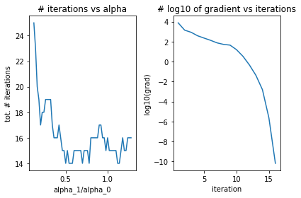
For flag manifolds, we optimize the function over matrices . Here, is a positive-definite matrix, are two positive integers, is a partition of with , for positive numbers . This cost function is invariant under the action of of , thus could be considered as a function on the flag manifold . The Euclidean gradient is , and the Euclidean Hessian is computed by routine matrix calculus. For testing, we consider and use a trust-region solver. In this case, there is no noticeable variation in time when different values of are used, typically a few seconds on a free colab engine in the notebook colab/SimpleFlag.ipynb in [21]. Convergence is achieved after typically trust-region iterations, with small alpha requiring more outer iterations. The convergence is superlinear as seen in fig. 1.
For another test of the Riemannian optimization framework, we consider a nonlinear weighted PCA (principal component analysis) problem, which could be solved by optimizing over the positive-semidefinite matrix manifold. Given a symmetric matrix and a weight vector we want to minimize the cost function
of a positive-semidefinite matrix , with . Here, denotes the diagonal matrix . When has identical weight , , expanding the cost function, we need to minimize in and , which implies . Thus, the problem is optimizing over the Stiefel manifold (actually over the Grassmann manifold as the function is invariant when is multiplied on the right by an orthogonal matrix), which could be considered as a quadratic PCA problem. When has non identical weights, it is difficult to reduce the problem to a Stiefel manifold, hence we optimize over the positive-semidefinite manifold, with a trust-region solver.
The cost function from extends to , and is denoted by . For a horizontal tangent vector at
We have , and similar equalities for give us
The ambient Hessian follows from a directional derivative calculation
The Riemannian gradient is computed as , with is given by eq. 8.4, the Riemannian Hessian is computed from eq. 2.11, with all components given in theorem 3. We use the built-in trust region solver in [27].
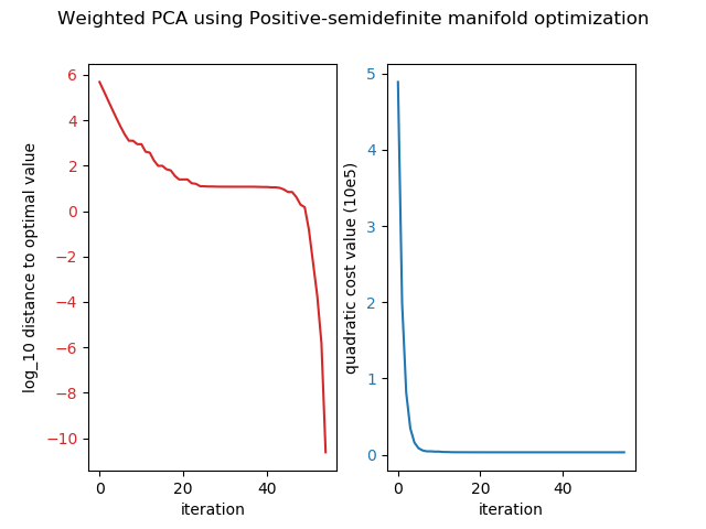
In our experiment (implemented in the notebook colab/WeightedPCA.ipynb in [20]), we take , with and generated randomly. To find the optimum , we optimize with , with is for the first iterations, for the next and for the remaining iterations. This choice of comes from our limited experiments, we find varying has a strong effect on the speed of convergence, and updating as such gives better convergence rates than a static . Philosophically, the small starting could be thought of as focusing first on aligning the subspace. The convergence graph is summarized in fig. 2. We hope to revisit the topic with a more systematic study in future works.
10. Conclusion
In this paper, we have proposed a framework to compute the Riemannian gradient, Levi-Civita connection, and the Riemannian Hessian effectively when the constraints, the symmetry of the problem, and the metrics are given analytically and have applied the framework to several manifolds important in applications. We look to apply the results in this paper to several problems in optimization and statistical learning. The optimization platform for positive-semidefinite matrices should help to learn sparse plus low-rank probability densities in statistical problems. We hope the research community will find the method useful in future works.
References
- [1] P.-A. Absil, R. Mahony, and R. Sepulchre, Optimization algorithms on matrix manifolds, Princeton University Press, Princeton, NJ, USA, 2007.
- [2] P. A. Absil, Robert Mahony, and Jochen Trumpf, An extrinsic look at the Riemannian Hessian, Geometric Science of Information (Frank Nielsen and Frédéric Barbaresco, eds.), Springer Berlin Heidelberg, 2013, pp. 361–368.
- [3] Roy L. Adler, Jean-Pierre Dedieu, Joseph Y. Margulies, Marco Martens, and Mike Shub, Newton’s method on Riemannian manifolds and a geometric model for the human spine, IMA Journal of Numerical Analysis 22 (2002), no. 3, 359–390.
- [4] A. C. Aitken, On Least Squares and Linear Combination of Observations, Proceedings of the Royal Society of Edinburgh 55 (1936), 42–48.
- [5] R. H. Bartels and G. W. Stewart, Solution of the matrix equation ax + xb = c [f4], Commun. ACM 15 (1972), no. 9, 820826.
- [6] Rajendra Bhatia and Peter Rosenthal, How and why to solve the operator equation AX - XB = Y, Bulletin of the London Mathematical Society 29 (1997), 1 – 21.
- [7] Silvère Bonnabel and Rodolphe Sepulchre, Riemannian metric and geometric mean for positive semidefinite matrices of fixed rank, SIAM Journal on Matrix Analysis and Applications 31 (2010), no. 3, 1055–1070.
- [8] N. Boumal, B. Mishra, P.-A. Absil, and R. Sepulchre, Manopt, a Matlab toolbox for optimization on manifolds, Journal of Machine Learning Research 15 (2014), 1455–1459.
- [9] Alan Edelman, Tomás A. Arias, and Steven T. Smith, The geometry of algorithms with orthogonality constraints, SIAM J. Matrix Anal. Appl. 20 (1999), no. 2, 303–353.
- [10] D. Gabay, Minimizing a differentiable function over a differential manifold, Journal of Optimization Theory and Applications 37 (1982), no. 2, 177–219.
- [11] Knut Hüper, Irina Markina, and Fátima Silva Leite, A Lagrangian approach to extremal curves on Stiefel manifolds, Journal of Geometric Mechanics 13 (2021), no. 1, 55–72.
- [12] Ben Jeuris, Raf Vandebril, and Bart Vandereycken, A survey and comparison of contemporary algorithms for computing the matrix geometric mean, Electron. Trans. Numer. Anal. 39 (2012), 379–402.
- [13] M. Journée, F. Bach, P.-A. Absil, and R. Sepulchre, Low-rank optimization on the cone of positive semidefinite matrices, SIAM Journal on Optimization 20 (2010), no. 5, 2327–2351.
- [14] H. Kasai and B. Mishra, Low-rank tensor completion: a Riemannian manifold preconditioning approach, Proceedings of Machine Learning Research, vol. 48, 20–22 Jun 2016, pp. 1012–1021.
- [15] J. H. Manton, Optimization algorithms exploiting unitary constraints, IEEE Transactions on Signal Processing 50 (2002), no. 3, 635–650.
- [16] Nina Miolane, Alice Le Brigant, Johan Mathe, Benjamin Hou, Nicolas Guigui, Yann Thanwerdas, Stefan Heyder, Olivier Peltre, Niklas Koep, Hadi Zaatiti, Hatem Hajri, Yann Cabanes, Thomas Gerald, Paul Chauchat, Christian Shewmake, Bernhard Kainz, Claire Donnat, Susan Holmes, and Xavier Pennec, Geomstats: A Python Package for Riemannian Geometry in Machine Learning, 2020.
- [17] Bamdev Mishra, Gilles Meyer, Silvère Bonnabel, and Rodolphe Sepulchre, Fixed-rank matrix factorizations and Riemannian low-rank optimization, Computational Statistics 29 (2014), 591, 621.
- [18] Bamdev. Mishra and Rodolphe. Sepulchre, Riemannian preconditioning, SIAM Journal on Optimization 26 (2016), no. 1, 635–660.
- [19] D. Nguyen, Closed-form geodesics and trust-region method to calculate Riemannian logarithms on Stiefel and its quotient manifolds, 2021.
- [20] Du Nguyen, Project ManNullRange, https://github.com/dnguyend/ManNullRange, 2020.
- [21] by same author, Project SimpleFlag, https://github.com/dnguyend/SimpleFlag, 2021.
- [22] Yasunori Nishimori, Shotaro Akaho, and Mark D. Plumbley, Riemannian optimization method on the flag manifold for independent subspace analysis, Independent Component Analysis and Blind Signal Separation (Justinian Rosca, Deniz Erdogmus, José C. Príncipe, and Simon Haykin, eds.), Springer Berlin Heidelberg, 2006, pp. 295–302.
- [23] B. O’Neill, Semi-riemannian geometry with applications to relativity, Pure and Applied Mathematics, vol. 103, Academic Press, Inc, New York, NY, 1983.
- [24] X. Pennec, P. Fillard, and N. Ayache, A Riemannian Framework for Tensor Computing, Int J Comput Vision (2006), 41–66.
- [25] S. T. Smith, Covariance, subspace, and intrinsic Cramér–-Rao bounds, IEEE Transactions on Signal Processing 53 (2005), no. 5, 1610–1630.
- [26] Suvrit Sra and Reshad Hosseini, Conic geometric optimization on the manifold of positive definite matrices, SIAM Journal on Optimization 25 (2015), no. 1, 713–739.
- [27] James Townsend, Niklas Koep, and Sebastian Weichwald, Pymanopt: A Python toolbox for optimization on manifolds using automatic differentiation, J. Mach. Learn. Res. 17 (2016), no. 137, 1–5.
- [28] Bart Vandereycken, P.-A. Absil, and Stefan Vandewalle, A Riemannian geometry with complete geodesics for the set of positive semidefinite matrices of fixed rank, IMA Journal of Numerical Analysis 33 (2012), no. 2, 481–514.
- [29] Ke Ye, Ken Sze-Wai Wong, and Lek-Heng Lim, Optimization on flag manifolds, Mathematical Programming, Series A (2021).