Two critical times for the SIR model

Abstract

We consider the SIR model and study the first time the number of infected individuals begins to decrease and the first time this population is below a given threshold. We interpret these times as functions of the initial susceptible and infected populations and characterize them as solutions of a certain partial differential equation. This allows us to obtain integral representations of these times and in turn to estimate them precisely for large populations.

1 Introduction

The susceptible, infected, and recovered (SIR) model in epidemiology involves the system of ODE

$$\begin{cases}\dot{S}=-\beta SI\\ \dot{I}=\beta SI-\gamma I.\end{cases}$$ (1.1)

Here $S,I:[0,\infty)\rightarrow[0,\infty)$ denote the susceptible and infected compartments of a given population in the presence of an infectious disease. If $N$ is the size of the population, then

$$R(t)=N-S(t)-I(t)$$

is the recovered compartment of the population at time $t$. The parameters $\beta>0$ and $\gamma>0$ are the infected and recovery rates per unit time, respectively.

We note that for given initial conditions $S(0),I(0)\geq 0$, there is a unique solution of the SIR ODE. Indeed, a local solution pair $S,I:[0,T)\rightarrow\mathbb{R}$ of (1.1) exists by standard ODE theory (see for example section I.2 [3]). As

$$S(t)=S(0)e^{\displaystyle-\beta\int^{t}_{0}I(\tau)d\tau}\;\text{and}\;\;I(t)=I(0)e^{\displaystyle\int^{t}_{0}(\beta S(\tau)-\gamma)d\tau}$$ (1.2)

for $t\in[0,T)$, $S$ and $I$ are nonnegative. By (1.1), $\frac{d}{dt}(S+I)(t)=-\gamma I(t)\leq 0$. Therefore,

$$S(t)+I(t)\leq S(0)+I(0)$$

for all $t\in[0,T)$. As a result, $S$ and $I$ are uniformly bounded. Consequently it is possible to continue this solution to all of $[0,\infty)$ (section I.2 [3]). And in view of (1.2), $S(t)$ is positive for all $t>0$ provided $S(0)>0$ and likewise for $I(t)$.

Let us recall three important properties about each solution $S,I:[0,\infty)\rightarrow(0,\infty)$ of the SIR ODE. For more details on these facts, we refer the reader to section 2.2 of [4] and section 9.2 of [1].

Integrability. Although $S$ and $I$ are not explicitly known, they are integrable in sense that

$$S(t)+I(t)-\frac{\gamma}{\beta}\ln S(t)=S(0)+I(0)-\frac{\gamma}{\beta}\ln S(0)$$ (1.3)

for each time $t\geq 0$. That is, the path $t\mapsto(S(t),I(t))$ belongs to a level set of the function

$$\psi(x,y):=x+y-(\gamma/\beta)\ln x.$$

In particular, we may consider $I$ as a function of $S$.

Decay of infected individuals. The number of infected individuals tends to $0$ as $t\rightarrow\infty$

$$\lim_{t\rightarrow\infty}I(t)=0.$$ (1.4)

In particular, for any given threshold $\mu>0$, there is a finite time $t$ such that the number of infected individuals falls below $\mu$

$$I(t)\leq\mu.$$

In what follows, we will write $u\geq 0$ for the first time in which $I$ falls below $\mu$.

Infected individuals eventually decrease. There is a time $v\geq 0$ for which

$$I [v,\infty)$$ is decreasing on .

Since $I$ is a positive function and $\dot{I}(t)=(\beta S(t)-\gamma)I(t)$, $v$ can be taken to be the first time $t$ that the number of susceptible individuals falls below the ratio of the recovery and infected rates

$$S(t)\leq\frac{\gamma}{\beta}.$$ (1.5)

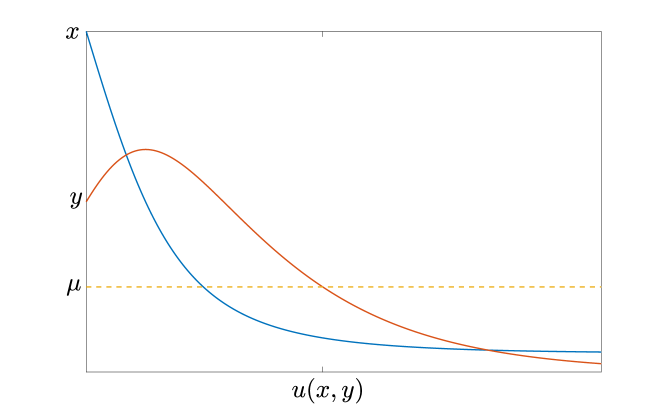
Figure 1: Plot of the solution pair $S,I$ of (1.1) with $S(0)=x$ and $I(0)=y$. $S(t)$ is shown in blue and $I(t)$ is shown in red. Note that $u(x,y)$ is the first time $t$ such that $I(t)\leq\mu$.

In this note, we will study the times $u$ and $v$ mentioned above as functions of the initial conditions $S(0)$ and $I(0)$. First, we will fix a threshold

$$\mu>0$$

and consider

$$u(x,y):=\min\{t\geq 0:I(t)\leq\mu\}$$ (1.6)

for $x,y\geq 0$. Here $S,I$ are solutions of (1.1) with $S(0)=x$ and $I(0)=y$. As $u(x,y)=0$ when $0\leq y<\mu$, we will focus on the values of $u(x,y)$ for $x\geq 0$ and $y\geq\mu$.

We’ll see that $u$ is a smooth function on $(0,\infty)\times(\mu,\infty)$ which satisfies the PDE

$$\beta xy\partial_{x}u+(\gamma-\beta x)y\partial_{y}u=1$$ (1.7)

and boundary condition

$$u(x,\mu)=0,\;x\in[0,\gamma/\beta].$$ (1.8)

Moreover, we will also use $\psi$ to write a representation formula for $u$. To this end, we note that for $x>0,y\geq\mu$ and there is a unique $a(x,y)\in(0,\gamma/\beta]$ such that

$$\psi(x,y)=\psi(a(x,y),\mu).$$

Further, $a(x,y)<x$ when $x>\gamma/\beta$ or $y>\mu$. These fact follows easily from the definition of $\psi$; Figure 3 below also provides a schematic.

A basic result involving $u$ is as follows.

Theorem 1.1.

The function $u$ defined in (1.6) has the following properties.

1. $u$ is continuous on $[0,\infty)\times[\mu,\infty)$ and is smooth in $(0,\infty)\times(\mu,\infty)$.

2. $u$ is the unique solution of (1.7) in $(0,\infty)\times(\mu,\infty)$ which satisfies the boundary condition (1.8).

3. For each $x>0$ and $y\geq\mu$,

   $$u(x,y)=\int^{x}_{a(x,y)}\frac{dz}{\beta z\left((\gamma/\beta)\ln z-z+\psi(x,y)\right)}.$$ (1.9)

Next, we will study

$$v(x,y):=\min\{t\geq 0:S(t)\leq\gamma/\beta\}$$ (1.10)

for $x\geq 0$ and $y\geq 0$. Above, we are assuming that $S,I$ is the solution pair of the SIR ODE (1.1) with $S(0)=x$ and $I(0)=y$. Note that $v(x,y)$ records the first time $t$ that $I(t)$ starts to decrease. Since

$$\begin{cases}v(x,y)=0\;\text{ for $0\leq x\leq\gamma/\beta$ and}\\ \\ v(x,0)=\infty\;\text{ for $x>\gamma/\beta$},\end{cases}$$ (1.11)

we will focus on the values of $v(x,y)$ for $x>\gamma/\beta$ and $y>0$.

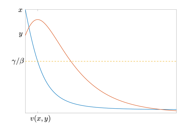
Figure 2: The solution pair $S,I$ of (1.1) with $S(0)=x$ and $I(0)=y$. $S(t)$ is shown in blue and $I(t)$ is shown in red. Note that $v(x,y)$ is the first time $S(t)\leq\gamma/\beta$ which is also the same time that $I$ starts to decrease.

The methods we use to prove Theorem 1.1 extend analogously to $v$. In particular, $v$ satisfies the same PDE as $u$ with the boundary condition

$$v(\gamma/\beta,y)=0,\;y\in(0,\infty).$$ (1.12)

Almost in parallel with Theorem 1.1, we have the subsequent assertion.

Theorem 1.2.

The function $v$ defined in (1.10) has the following properties.

1. $v$ is continuous on $[\gamma/\beta,\infty)\times(0,\infty)$ and is smooth in $(\gamma/\beta,\infty)\times(0,\infty)$.

2. $v$ is the unique solution of (1.7) in $(\gamma/\beta,\infty)\times(0,\infty)$ which satisfies the boundary condition (1.12).

3. For each $x\geq\gamma/\beta$ and $y>0$,

   $$v(x,y)=\int^{x}_{\gamma/\beta}\frac{dz}{\beta z\left((\gamma/\beta)\ln z-z+\psi(x,y)\right)}.$$ (1.13)

We will then use the above representation formulae to show how to precisely estimate the $u(x,y)$ and $v(x,y)$ when $x+y$ is large.

Theorem 1.3.

Define $u$ by (1.6) and $v$ by (1.10). Then

$$\lim_{\begin{subarray}{c}x+y\rightarrow\infty\\ x\geq 0,\;y\geq\mu\end{subarray}}\frac{\displaystyle u(x,y)}{\displaystyle\frac{1}{\gamma}\ln\left(\frac{x+y}{\mu}\right)}=1$$ (1.14)

and

$$\lim_{\begin{subarray}{c}x+y\rightarrow\infty\\ x>\gamma/\beta,\;y>0\end{subarray}}\frac{\displaystyle\beta(x-\gamma/\beta+y)}{\displaystyle\ln\left[\left(\frac{x}{\gamma/\beta}\right)\left(\frac{x-\gamma/\beta}{y}+1\right)\right]}\cdot v(x,y)=1.$$ (1.15)

The limit (1.14) implies that $u(x,y)$ tends to $\infty$ as $x+y\rightarrow\infty$. This limit also reduces to an exact formula when $x=0$. In this case, $S(t)=0$ and $I(t)=ye^{-\gamma t}$, so

$$u(0,y)=\frac{1}{\gamma}\ln\left(\frac{y}{\mu}\right).$$

Alternatively, the limit (1.15) implies that $v(x,y)$ tends to $0$ as $x+y\rightarrow\infty$ with $y\geq\delta$ for each $\delta>0$. This will be a crucial element of our proof of (1.14).

This paper is organized as follows. In section 2, we will study $u$ and prove Theorem 1.1. Then in section 3, we will indicate what changes are necessary so that our proof of Theorem 1.1 adapts to Theorem 1.2. Finally, we will prove Theorem 1.3 in section 4. We also would like to acknowledge that this material is based upon work supported by the NSF under Grants No. DMS-1440140 and DMS-1554130, NSA under Grant No. H98230-20-1-0015, and the Sloan Foundation under Grant No. G-2020-12602 while the authors participated in the ADJOINT program hosted by MSRI.

2 The first time $I(t)\leq\mu$

This section is dedicated to proving Theorem 1.1. We will begin with an elementary upper bound on $u$.

Lemma 2.1.

For each $x\geq 0$ and $y\geq\mu$,

$$u(x,y)\leq\frac{x+y}{\gamma\mu}.$$ (2.1)

Proof.

Let $S,I$ be the solution pair of the SIR ODE (1.1) with $S(0)=x$ and $I(0)=y$. Since $\frac{d}{dt}(S+I)(t)=-\gamma I(t)\leq 0$,

$$\int^{t}_{0}\gamma I(\tau)d\tau+S(t)+I(t)=x+y.$$

Choosing $t=u(x,y)$ and noting that $I(\tau)\geq\mu$ for $0\leq\tau\leq u(x,y)$ gives

$$u(x,y)\gamma\mu\leq\int^{u(x,y)}_{0}\gamma I(\tau)d\tau\leq x+y.$$

∎

Next we observe that $I$ is always decreasing at the time it reaches the threshold $\mu$.

Lemma 2.2.

Let $x>0$, $y>\mu$, and suppose $S,I$ is the solution of (1.1) with $S(0)=x$ and $I(0)=y$. Then

$$\dot{I}(u(x,y))<0.$$

Proof.

As $\dot{I}(t)=(\beta S(t)-\gamma)I(t)$, it suffices to show

$$\beta S(u(x,y))-\gamma<0.$$ (2.2)

If $\beta x\leq\gamma$, then $\beta S(t)<\gamma$ for all $t>0$ since $S$ is decreasing. Consequently, (2.2) holds for $t=u(x,y)$. Alternatively, if $\beta x>\gamma$, then $I$ is nonincreasing on the interval $[0,v(x,y)]$ and

$$\beta S(v(x,y))-\gamma=0.$$

In particular, $I(v(x,y))\geq y>\mu$. Thus, $v(x,y)<u(x,y)$. As $S$ is decreasing,

$$\beta S(u(x,y))-\gamma<\beta S(v(x,y))-\gamma=0.$$

∎

Remark 2.3.

Since $v(x,y)=0$ for $x\in[0,\gamma/\beta]$, it also follows from this proof that

$$v(x,y)\leq u(x,y)$$ (2.3)

for each $x\geq 0$ and $y\geq\mu$.

We will also need to verify that solutions of the SIR ODE (1.1) depend continuously on their initial conditions.

Lemma 2.4.

Suppose $x^{k}\geq 0$ and $y^{k}\geq 0$, and let $S^{k},I^{k}$ be the solution of (1.1) with $S^{k}(0)=x^{k}$ and $I^{k}(0)=y^{k}$ for each $k\in\mathbb{N}$. If $x^{k}\rightarrow x$ and $y^{k}\rightarrow y$ as $k\rightarrow\infty$, then

$$S(t)=\lim_{k\rightarrow\infty}S^{k}(t_{k})\quad\text{and}\quad I(t)=\lim_{k\rightarrow\infty}I^{k}(t_{k})$$ (2.4)

for each sequence $t_{k}\geq 0$ such that $t_{k}\rightarrow t$. Here $S,I$ is the solution of (1.1) with $S(0)=x$ and $I(0)=y$.

Proof.

We note that $S^{k}$ and $I^{k}$ are nonnegative functions with

$$S^{k}(t)+I^{k}(t)\leq x^{k}+y^{k}$$

for all $t\geq 0$. Thus, $S^{k}$ and $I^{k}$ are uniformly bounded independently of $k\in\mathbb{N}$. In view of (1.1), we additionally have

$$|\dot{S}^{k}(t)|\leq\beta(x^{k}+y^{k})^{2}$$

and

$$|\dot{I}^{k}(t)|\leq\beta(x^{k}+y^{k})^{2}+\gamma(x^{k}+y^{k})$$

for each $t\geq 0$. Consequently, $S^{k},I^{k}$ are uniformly equicontinuous on $[0,\infty)$.

The Arzelà-Ascoli theorem then implies there are subsequences $S^{k_{j}}$ and $I^{k_{j}}$ converging uniformly on any bounded subinterval of $[0,\infty)$ to continuous functions $S$ and $I$, respectively. Observe

$$S^{k}(t)=x^{k}-\int^{t}_{0}\beta S^{k}(\tau)I^{k}(\tau)d\tau\;\;\text{and}\;\;I^{k}(t)=y^{k}+\int^{t}_{0}(\beta S^{k}(\tau)-\gamma)I^{k}(\tau)d\tau$$ (2.5)

for each $t\geq 0$. Letting $k=k_{j}\rightarrow\infty$ and employing the uniform convergence of $S^{k_{j}}$ and $I^{k_{j}}$ on $[0,t]$ for each $t\geq 0$, we see that $S,I$ is the solution of (1.1) with $S(0)=x$ and $I(0)=y$. As this limit is independent of the subsequence, it must be that $S^{k}$ and $I^{k}$ converge to $S$ and $I$, respectively, locally uniformly on $[0,\infty)$. As a result, we conclude (2.4). ∎

In our proof of Theorem 1.1 below, we will employ the flow of the SIR ODE (1.1). This is the mapping

$$\Phi:[0,\infty)^{3}\rightarrow[0,\infty)^{2};(x,y,t)\mapsto(S(t),I(t))$$ (2.6)

where $S,I$ is the solution pair of (1.1) with $S(0)=x$ and $I(0)=y$. We will also write $\Phi=(\Phi_{1},\Phi_{2})$ so that

$$\Phi_{1}(x,y,t)=S(t)\;\;\text{and}\;\;\Phi_{2}(x,y,t)=I(t).$$ (2.7)

A direct corollary of Lemma 2.4 is that $\Phi$ is a continuous mapping. With a bit more work, it can also be shown that $\Phi:(0,\infty)^{3}\rightarrow[0,\infty)^{2}$ is smooth (exercise 3.2 in Chapter 1 of [3], Chapter 1 section 7 of [2]).

Proof of Theorem 1.1.

$(i)$ Suppose $x^{k}\geq 0$ and $y^{k}\geq\mu$ with $x^{k}\rightarrow x$ and $y^{k}\rightarrow y$ as $k\rightarrow\infty$. By Lemma (2.1), $u(x^{k},y^{k})$ is uniformly bounded. We can then select a subsequence $u(x^{k_{j}},y^{k_{j}})$ which converges to some $t\geq 0$. From the definition of $u$, we also have

$$\Phi_{2}(x^{k},y^{k},u(x^{k},y^{k}))=\mu$$ (2.8)

for each $k\in\mathbb{N}$. Since $\Phi_{2}$ is continuous, we can send $k=k_{j}\rightarrow\infty$ in (2.8) to get

$$\Phi_{2}(x,y,t)=\mu.$$

As $y\geq\mu$, the limit $t$ is equal to $u(x,y)$. Because this limit is independent of the subsequence $u(x^{k_{j}},y^{k_{j}})$, it must be that

$$u(x,y)=\lim_{k\rightarrow\infty}u(x^{k},y^{k}).$$ (2.9)

It follows that $u$ is continuous on $[0,\infty)\times[\mu,\infty)$.

Let $x>0$ and $y>\mu$ and recall that $\Phi_{2}(x,y,u(x,y))=\mu$. By Lemma 2.2,

$$\partial_{t}\Phi_{2}(x,y,u(x,y))<0.$$ (2.10)

Since $\Phi_{2}$ is smooth in a neighborhood of $(x,y,u(x,y))$, the implicit function theorem implies that $u$ is smooth in a neighborhood of $(x,y)$. We conclude that $u$ is smooth in $(0,\infty)\times(\mu,\infty)$.

$(ii)$ Fix $x>0$ and $y>\mu$, and let $S,I$ be the solution of (1.1) with $S(0)=x$ and $I(0)=y$. Observe that for each $0\leq t<u(x,y)$,

$$u(S(t),I(t)) =\min\{\tau\geq 0:I(t+\tau)\leq\mu\}$$

$$=\min\{s\geq t:I(s)\leq\mu\}-t$$

$$=u(x,y)-t.$$

Therefore,

$$1 =-\left.\frac{d}{dt}u(S(t),I(t))\right|_{t=0}$$ (2.11)

$$=\left.\Big{[}\beta S(t)I(t)\partial_{x}u(S(t),I(t))+(\gamma-\beta S(t))I(t)\partial_{y}u(S(t),I(t))\Big{]}\right|_{t=0}$$ (2.12)

$$=\beta xy\partial_{x}u(x,y)+(\gamma-\beta x)y\partial_{y}u(x,y).$$ (2.13)

We conclude that $u$ satisfies (1.7).

Now suppose $w$ is a solution of (1.7) which satisfies the boundary condition (1.8). Note

$$\frac{d}{dt}w(S(t),I(t))=-\Big{[}\beta S(t)I(t)\partial_{x}w(S(t),I(t))+(\gamma-\beta S(t))I(t)\partial_{y}w(S(t),I(t))\Big{]}=-1$$

for $0\leq t<u(x,y)$. Integrating this equation from $t=0$ to $t=u(x,y)$ gives

$$w(S(u(x,y)),I(u(x,y)))-w(x,x)=-u(x,y).$$

Since $I(u(x,y))=\mu$, $\beta S(u(x,y))\leq\gamma$, and $w(S(u(x,y)),\mu)=0$, it follows that $w(x,y)=u(x,y)$. Therefore, $u$ is the unique solution of the PDE (1.7) which satisfies the boundary condition (1.8).

$(iii)$ Suppose either $x>0$ and $y>\mu$ or $x>\gamma/\beta$ and $y=\mu$. We recall that $a=a(x,y)\in(0,\gamma/\beta]$ is the unique solution of

$$\psi(x,y)=\psi(a,\mu).$$

It is also easy to check that

$$\frac{\gamma}{\beta}\ln z-z+\psi(x,y)>\mu$$

for $a<z<x$. See Figure 3 for an example.

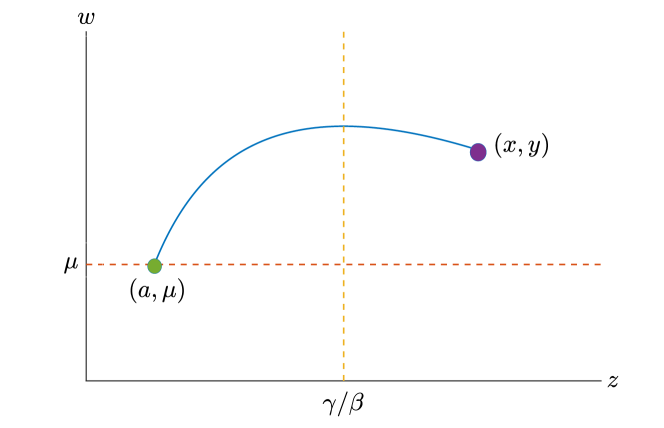
Figure 3: Graph of $w=(\gamma/\beta)\ln z-z+\psi(x,y)$ for $a\leq z\leq x$. Here $x>0$, $y>\mu$, and $a=a(x,y)\in(0,\gamma/\beta]$ is the unique solution of $\psi(x,y)=\psi(a,\mu)$. Also note that this graph is a subset of the level set $\{(z,w)\in(0,\infty)^{2}:\psi(z,w)=\psi(x,y)\}$.

Since $u$ solves the PDE (1.7),

$$\frac{d}{dz}u\left(z,\frac{\gamma}{\beta}\ln z-z+\psi(x,y)\right) =\left.\frac{\beta zy\partial_{x}u(z,y)+(\gamma-\beta z)y\partial_{y}u(z,y)}{\beta zy}\right|_{y=\frac{\gamma}{\beta}\ln z-z+\psi(x,y)}$$ (2.14)

$$=\frac{1}{\beta z\left(\frac{\gamma}{\beta}\ln z-z+\psi(x,y)\right)}$$ (2.15)

for $a<z<x$. Integrating from $z=a$ to $z=x$ and using the boundary condition (1.8) gives

$$u(x,y)=\int^{x}_{a}\frac{dz}{\beta z\left((\gamma/\beta)\ln z-z+\psi(x,y)\right)}.$$

∎

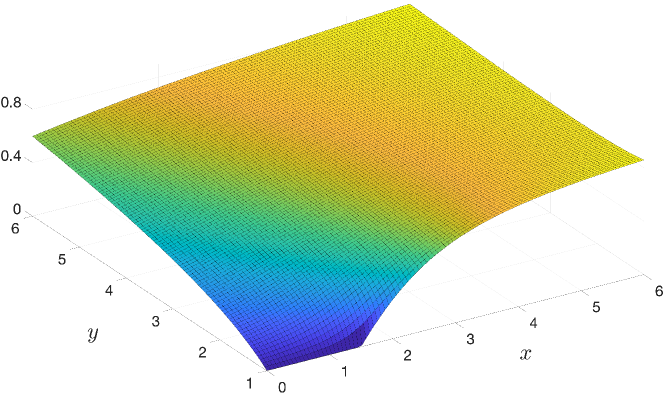
Figure 4: Numerical approximation of the function $u(x,y)$ for $(x,y)\in[0,6]\times[1,5]$. Here $\mu=1$, $\beta=2$, and $\gamma=3$.

3 The first time $S(t)\leq\gamma/\beta$

We will briefly point out what needs to be adapted from the previous section so that we can conclude Theorem 1.2 involving $v$. We first note that $v$ is locally bounded in $[\gamma/\beta,\infty)\times(0,\infty)$.

Lemma 3.1.

For each $x\geq\gamma/\beta$ and $y>0$,

$$v(x,y)\leq\frac{\ln x-\ln(\gamma/\beta)}{\beta y}.$$ (3.1)

Proof.

Let $S,I$ denote the solution of (1.1) with $S(0)=x$ and $I(0)=y$. Since $I(t)$ is increasing on $t\in[0,v(x,y)]$, $I(t)\geq y$ for $t\in[0,v(x,y)]$. In view of (1.2)

$$\frac{\gamma}{\beta}=S(v(x,y))=xe^{\displaystyle-\beta\int^{v(x,y)}_{0}I(\tau)d\tau}\leq xe^{-\beta yv(x,y)}.$$ (3.2)

Taking the natural logarithm and rearranging leads to $v(x,y)\leq(\ln x-\ln(\gamma/\beta))/\beta y$, which is what we wanted to show. ∎

The next assertion follows since $S$ is decreasing whenever $I$ is initially positive. The main point of stating this lemma is to make an analogy with Lemma 2.2.

Lemma 3.2.

Let $x\geq\gamma/\beta$ and $y>0$, and suppose $S,I$ is the solution of (1.1) with $S(0)=x$ and $I(0)=y$. Then

$$\dot{S}(v(x,y))<0.$$ (3.3)

Having established Lemmas 3.1 and 3.2, we can now argue virtually the same way we did in the previous section to conclude Theorem 1.2. Consequently, we will omit a proof.

Figure 5: Numerical approximation of the function $v(x,y)$ for $(x,y)\in[1,20]\times[1/2,5]$. Here $\beta=\gamma=3$.

4 Asymptotics

In this final section, we will derive a few estimates on $u(x,y)$ and $v(x,y)$ that we will need to prove Theorem 1.3. First, we record an upper and lower bound on $u$.

Lemma 4.1.

If $x\geq 0$ and $y\geq\mu$, then

$$u(x,y)\geq\frac{1}{\gamma}\ln\left(\frac{x+y}{\gamma/\beta+\mu}\right).$$ (4.1)

If $x\in[0,\gamma/\beta)$ and $y\geq\mu$, then

$$u(x,y)\leq\frac{\ln(y/\mu)}{\gamma-\beta x}.$$ (4.2)

Proof.

Set

$$w(x,y)=\frac{1}{\gamma}\ln\left(\frac{x+y}{\gamma/\beta+\mu}\right).$$

Observe that for each $x\geq 0$ and $y\geq\mu$,

$$\beta xy\partial_{x}w+(\gamma-\beta x)y\partial_{y}w=\frac{1}{\gamma}\frac{\beta xy+(\gamma-\beta x)y}{x+y}=\frac{y}{x+y}\leq 1.$$ (4.3)

Now fix $x\geq 0$ and $y\geq\mu$ and suppose $S,I$ is the solution of (1.1) with $S(0)=x$ and $I(0)=y$. By our computation above,

$$\frac{d}{dt}w(S(t),I(t))=-\Big{[}\beta S(t)I(t)\partial_{x}w(S(t),I(t))+(\gamma-\beta S(t))I(t)\partial_{y}w(S(t),I(t))\Big{]}\geq-1$$

for $0\leq t\leq u(x,y)$. And integrating this inequality from $t=0$ to $t=u(x,y)$ gives

$$w(S(u(x,y)),\mu)-w(x,y)\geq-u(x,y).$$ (4.4)

Since $S(u(x,y))\leq\gamma/\beta$,

$$w(S(u(x,y)),\mu)=\frac{1}{\gamma}\ln\left(\frac{S(u(x,y))+\mu}{\gamma/\beta+\mu}\right)\leq 0.$$

Combined with (4.4) this implies $u(x,y)\geq w(x,y)$. We conclude (4.1).

Now suppose $\beta x<\gamma$ and $y>\mu$. By (1.2),

$$\mu=I(u(x,y))=ye^{\displaystyle\int^{u(x,y)}_{0}(\beta S(\tau)-\gamma)d\tau}\leq ye^{(\beta x-\gamma)u(x,y)}.$$

Taking the natural logarithm and rearranging gives (4.2). ∎

Likewise, we can identify convenient upper and lower bounds for $v(x,y)$. To this end, we will exploit the fact that for each $x>\gamma/\beta$ and $y>0$

$$g(z)=(\gamma/\beta)\ln z-z+\psi(x,y)$$ (4.5)

is concave on the interval $\gamma/\beta\leq z\leq x.$ This implies

$$g(z)\geq\frac{g(\gamma/\beta)-y}{\gamma/\beta-x}(z-x)+g(x)=\left(\frac{\gamma}{\beta}\frac{\ln x-\ln(\gamma/\beta)}{x-\gamma/\beta}-1\right)(z-x)+y$$ (4.6)

and

$$g(z)\leq g^{\prime}(x)(z-x)+g(x)=\left(\frac{\gamma}{\beta x}-1\right)(z-x)+y$$ (4.7)

for $\gamma/\beta\leq z\leq x.$

Lemma 4.2.

Suppose $x>\gamma/\beta$ and $y>0$. Then

$$v(x,y)\leq\frac{\ln x-\ln(\gamma/\beta)-\ln y+\ln\left(x-\gamma/\beta+y-\frac{\gamma}{\beta}(\ln x-\ln(\gamma/\beta))\right)}{\beta\left(\displaystyle y+x\left(1-\frac{\gamma}{\beta}\frac{\ln x-\ln(\gamma/\beta)}{x-\gamma/\beta}\right)\right)}$$ (4.8)

and

$$v(x,y)\geq\frac{\ln x-\ln(\gamma/\beta)-\ln y+\ln\left(x-\gamma/\beta+y+\frac{\gamma}{\beta}(\frac{\gamma}{\beta x}-1)\right)}{\beta(\displaystyle x-\gamma/\beta+y)}.$$ (4.9)

Proof.

We will appeal to part $(iii)$ of Theorem 1.2 which asserts

$$v(x,y)=\int^{x}_{\gamma/\beta}\frac{dz}{\beta zg(z)}.$$ (4.10)

Here $g(z)$ is defined in (4.5). We will also employ the identity

$$\frac{d}{dz}\frac{\ln z-\ln(cz+d)}{d}=\frac{1}{z(cz+d)}.$$ (4.11)

By (4.6) and (4.11),

$$v(x,y) \leq\int^{x}_{\gamma/\beta}\frac{dz}{\displaystyle\beta z\left(\left(\frac{\gamma}{\beta}\frac{\ln x-\ln(\gamma/\beta)}{x-\gamma/\beta}-1\right)(z-x)+y\right)}$$ (4.12)

$$=\left.\frac{\ln z-\ln\left(\left(\displaystyle\frac{\gamma}{\beta}\frac{\displaystyle\ln x-\ln(\gamma/\beta)}{\displaystyle x-\gamma/\beta}-1\right)(z-x)+y\right)}{\beta\displaystyle\left(y+x\left(1-\frac{\gamma}{\beta}\frac{\ln x-\ln(\gamma/\beta)}{x-\gamma/\beta}\right)\right)}\right|^{z=x}_{z=\gamma/\beta}$$ (4.13)

$$=\frac{\ln x-\ln(\gamma/\beta)-\ln y+\ln\left(x-\gamma/\beta+y-\frac{\gamma}{\beta}(\ln x-\ln(\gamma/\beta))\right)}{\beta\left(\displaystyle y+x\left(1-\frac{\gamma}{\beta}\frac{\ln x-\ln(\gamma/\beta)}{x-\gamma/\beta}\right)\right)}.$$ (4.14)

Similarly, (4.7) and (4.11) give

$$v(x,y) \geq\int^{x}_{\gamma/\beta}\frac{dz}{\displaystyle\beta z\left(\left(\frac{\gamma}{\beta x}-1\right)(z-x)+y\right)}$$ (4.15)

$$=\left.\frac{\ln z-\ln\left(\left(\displaystyle\frac{\gamma}{\beta x}-1\right)(z-x)+y\right)}{\beta(\displaystyle x-\gamma/\beta+y)}\right|^{z=x}_{z=\gamma/\beta}$$ (4.16)

$$=\frac{\ln x-\ln(\gamma/\beta)-\ln y+\ln\left(x-\gamma/\beta+y+\frac{\gamma}{\beta}(\frac{\gamma}{\beta x}-1)\right)}{\beta(\displaystyle x-\gamma/\beta+y)}.$$ (4.17)

∎

Corollary 4.3.

For each $\delta>0$,

$$\lim_{\begin{subarray}{c}x+y\rightarrow\infty\\ x\geq 0,y\geq\delta\end{subarray}}v(x,y)=0.$$ (4.18)

Proof.

Choose sequences $x_{k}\geq 0$ and $y_{k}\geq\delta$ with $x_{k}+y_{k}\rightarrow\infty$ such that

$$\limsup_{\begin{subarray}{c}x+y\rightarrow\infty\\ x\geq\gamma/\beta,y\geq\delta\end{subarray}}v(x,y)=\lim_{k\rightarrow\infty}v(x_{k},y_{k}).$$

If $x_{k}\leq\gamma/\beta$ for infinitely many $k\in\mathbb{N}$, then $v(x_{k},y_{k})=0$ for infinitely many $k$ and

$$\lim_{k\rightarrow\infty}v(x_{k},y_{k})=0.$$ (4.19)

Otherwise, we may as well suppose that $x_{k}>\gamma/\beta$ for all $k\in\mathbb{N}$. In this case, (4.8) implies

$$v(x_{k},y_{k})\leq\frac{\ln x_{k}-\ln(\gamma/\beta)-\ln y_{k}+\ln\left(x_{k}-\gamma/\beta+y_{k}-\frac{\gamma}{\beta}(\ln x_{k}-\ln(\gamma/\beta))\right)}{\beta\left(\displaystyle y_{k}+x_{k}\left(1-\frac{\gamma}{\beta}\frac{\ln x_{k}-\ln(\gamma/\beta)}{x_{k}-\gamma/\beta}\right)\right)}$$ (4.20)

for all $k\in\mathbb{N}$.

If $x_{k}\rightarrow\infty$, then

$$\frac{\gamma}{\beta}\frac{\ln x_{k}-\ln(\gamma/\beta)}{x_{k}-\gamma/\beta}\leq\frac{1}{2}$$

for sufficiently large $k$. It follows that

$$v(x_{k},y_{k}) \leq\frac{\ln x_{k}-\ln(\gamma/\beta)-\ln y_{k}+\ln\left(x_{k}-\gamma/\beta+y_{k}-\frac{\gamma}{\beta}(\ln x_{k}-\ln(\gamma/\beta))\right)}{\beta\left(y_{k}+\frac{1}{2}x_{k}\right)}$$ (4.21)

$$\leq\frac{\ln x_{k}-\ln(\gamma/\beta)+\ln\left(\frac{x_{k}-\gamma/\beta}{y_{k}}+1\right)}{\beta\left(y_{k}+\frac{1}{2}x_{k}\right)}$$ (4.22)

$$\leq\frac{\ln x_{k}-\ln(\gamma/\beta)+\ln\left(\frac{x_{k}-\gamma/\beta}{\delta}+1\right)}{\beta\left(\delta+\frac{1}{2}x_{k}\right)}$$ (4.23)

for all large enough $k$. Therefore, (4.19) holds.

Alternatively, we can pass to a subsequence if necessary and suppose $x_{k}\leq c$ for all $k\in\mathbb{N}$ and $y_{k}\rightarrow\infty$. Lemma 3.1 then gives

$$v(x_{k},y_{k})\leq\frac{\ln c-\ln(\gamma/\beta)}{\beta y_{k}}\rightarrow 0.$$ (4.24)

As a result, (4.19) holds in all cases. It follows that

$$\limsup_{\begin{subarray}{c}x+y\rightarrow\infty\\ x\geq 0,y\geq\delta\end{subarray}}v(x,y)=0,$$

which in turn implies (4.18). ∎

We are now ready to prove Theorem 1.3 which asserts

$$\lim_{\begin{subarray}{c}x+y\rightarrow\infty\\ x\geq 0,\;y\geq\mu\end{subarray}}\frac{\displaystyle u(x,y)}{\displaystyle\frac{1}{\gamma}\ln\left(\frac{x+y}{\mu}\right)}=1$$ (4.25)

and

$$\lim_{\begin{subarray}{c}x+y\rightarrow\infty\\ x>\gamma/\beta,\;y>0\end{subarray}}\frac{\displaystyle\beta(x-\gamma/\beta+y)}{\displaystyle\ln\left[\left(\frac{x}{\gamma/\beta}\right)\left(\frac{x-\gamma/\beta}{y}+1\right)\right]}\cdot v(x,y)=1.$$ (4.26)

Proof of (4.25).

In view of (4.1),

$$\liminf_{\begin{subarray}{c}x+y\rightarrow\infty\\ x\geq 0\;y\geq\mu\end{subarray}}\frac{\displaystyle u(x,y)}{\displaystyle\frac{1}{\gamma}\ln\left(\frac{x+y}{\mu}\right)}\geq 1.$$

It follows that $u(x,y)\rightarrow\infty$ as $x+y\rightarrow\infty$ with $x\geq 0$ and $y\geq\mu$. In view of Corollary 4.18, we may select $N\in\mathbb{N}$ so large that

$$v(x,y)<u(x,y)$$

for all $x+y\geq N$ with $x\geq 0$ and $y\geq\mu$.

Suppose $x+y\geq N$ with $x\geq 0$ and $y\geq\mu$ and choose a time $t$ such that

$$v(x,y)<t<u(x,y).$$

Note that as $t>v(x,y)$,

$$S(t)<\frac{\gamma}{\beta}.$$

Here $S,I$ is the solution of the SIR ODE (1.1) with $S(0)=x$ and $I(0)=y$. By (4.2), we also have

$$u(x,y) =t+u(S(t),I(t))$$

$$\leq t+\frac{1}{\gamma-\beta S(t)}\ln\left(\frac{I(t)}{\mu}\right)$$

$$\leq t+\frac{1}{\gamma-\beta S(t)}\ln\left(\frac{x+y}{\mu}\right).$$ (4.27)

In addition, we can use (1.2) to find

$$S(t) =S(v(x,y))e^{\displaystyle-\beta\int^{t}_{v(x,y)}I(\tau)d\tau}$$ (4.28)

$$=\frac{\gamma}{\beta}e^{\displaystyle-\beta\int^{t}_{v(x,y)}I(\tau)d\tau}$$ (4.29)

$$\leq\frac{\gamma}{\beta}e^{-\beta\mu(t-v(x,y))}.$$ (4.30)

Here we used that $I(\tau)\geq\mu$ when $\tau\leq u(x,y)$. Therefore,

$$\gamma-\beta S(t)\geq\gamma\left(1-e^{-\beta\mu(t-v(x,y))}\right)$$

Combining this inequality with (4) gives

$$u(x,y)\leq t+\frac{1}{1-e^{-\beta\mu(t-v(x,y))}}\frac{1}{\gamma}\ln\left(\frac{x+y}{\mu}\right).$$ (4.31)

As a result,

$$\limsup_{\begin{subarray}{c}x+y\rightarrow\infty\\ x\geq 0\;y\geq\mu\end{subarray}}\frac{\displaystyle u(x,y)}{\displaystyle\frac{1}{\gamma}\ln\left(\frac{x+y}{\mu}\right)}\leq\frac{1}{1-e^{-\beta\mu t}}.$$

We conclude (4.25) upon sending $t\rightarrow\infty$. ∎

In our closing argument below, we will employ the elementary inequalities

$$\frac{1}{x}\leq\frac{\ln x-\ln(\gamma/\beta)}{x-\gamma/\beta}\leq\frac{\beta}{\gamma},$$ (4.32)

which hold for $x>\gamma/\beta$. They follow as the natural logarithm is concave.

Proof of (4.26).

By the upper bound (4.8),

$$\frac{\displaystyle\beta(x-\gamma/\beta+y)}{\displaystyle\ln\left[\left(\frac{x}{\gamma/\beta}\right)\left(\frac{x-\gamma/\beta}{y}+1\right)\right]}\cdot v(x,y)$$

$$\quad=\frac{\displaystyle\beta(x-\gamma/\beta+y)}{\displaystyle\ln x-\ln(\gamma/\beta)-\ln y+\ln\left(x-\gamma/\beta+y\right)}\cdot v(x,y)$$

$$\quad\leq\frac{\displaystyle\beta(x+y)}{\ln x-\ln(\gamma/\beta)-\ln y+\ln\left(x-\gamma/\beta+y-\frac{\gamma}{\beta}(\ln x-\ln(\gamma/\beta))\right)}\cdot v(x,y)$$

$$\quad\leq\frac{\displaystyle x+y}{\displaystyle y+x\left(1-\frac{\gamma}{\beta}\frac{\ln x-\ln(\gamma/\beta)}{x-\gamma/\beta}\right)}$$

$$\quad=\frac{\displaystyle 1}{\displaystyle 1-\frac{x}{x+y}\frac{\gamma}{\beta}\left(\frac{\ln x-\ln(\gamma/\beta)}{x-\gamma/\beta}\right)}.$$ (4.33)

We may select sequences $x_{k}>\gamma/\beta$ and $y_{k}>0$ with $x_{k}+y_{k}\rightarrow\infty$ and

$$\limsup_{\begin{subarray}{c}x+y\rightarrow\infty\\ x>\gamma/\beta,\;y>0\end{subarray}}\frac{x}{x+y}\frac{\gamma}{\beta}\left(\frac{\ln x-\ln(\gamma/\beta)}{x-\gamma/\beta}\right)=\lim_{k\rightarrow\infty}\frac{x_{k}}{x_{k}+y_{k}}\frac{\gamma}{\beta}\left(\frac{\ln x_{k}-\ln(\gamma/\beta)}{x_{k}-\gamma/\beta}\right).$$ (4.34)

If $x_{k}\rightarrow\infty$, then

$$0\leq\frac{x_{k}}{x_{k}+y_{k}}\frac{\gamma}{\beta}\left(\frac{\ln x_{k}-\ln(\gamma/\beta)}{x_{k}-\gamma/\beta}\right)\leq\frac{\gamma}{\beta}\frac{\ln x_{k}}{x_{k}-\gamma/\beta}\rightarrow 0.$$

Alternatively, $x_{k}$ has a bounded subsequence. Passing to a subsequence if necessary, we may assume that $x_{k}\leq c$ for some constant $c$. In which case, $y_{k}\rightarrow\infty$. Employing (4.32), we find

$$0\leq\frac{x_{k}}{x_{k}+y_{k}}\frac{\gamma}{\beta}\left(\frac{\ln x_{k}-\ln(\gamma/\beta)}{x_{k}-\gamma/\beta}\right)\leq\frac{x_{k}}{x_{k}+y_{k}}\leq\frac{c}{y_{k}}\rightarrow 0.$$

It follows that the limit in (4.34) is $0$. And in view of (4),

$$\limsup_{\begin{subarray}{c}x+y\rightarrow\infty\\ x>\gamma/\beta,\;y>0\end{subarray}}\frac{\displaystyle\beta(x-\gamma/\beta+y)}{\displaystyle\ln\left[\left(\frac{x}{\gamma/\beta}\right)\left(\frac{x-\gamma/\beta}{y}+1\right)\right]}\cdot v(x,y)\leq 1.$$

By the lower bound (4.9),

$$\frac{\displaystyle\beta(x-\gamma/\beta+y)v(x,y)}{\displaystyle\ln\left[\left(\frac{x}{\gamma/\beta}\right)\left(\frac{x-\gamma/\beta}{y}+1\right)\right]} =\frac{\displaystyle\beta(x-\gamma/\beta+y)v(x,y)}{\displaystyle\ln x-\ln(\gamma/\beta)-\ln y+\ln\left(x-\gamma/\beta+y\right)}$$

$$\quad\geq\frac{\ln x-\ln(\gamma/\beta)-\ln y+\ln\left(x-\gamma/\beta+y+\frac{\gamma}{\beta}(\frac{\gamma}{\beta x}-1)\right)}{\displaystyle\ln x-\ln(\gamma/\beta)-\ln y+\ln\left(x-\gamma/\beta+y\right)}$$

$$\quad=1+\frac{\displaystyle\ln\left(\frac{x-\gamma/\beta+y+\frac{\gamma}{\beta}(\frac{\gamma}{\beta x}-1)}{x-\gamma/\beta+y}\right)}{\displaystyle\ln x-\ln(\gamma/\beta)-\ln y+\ln\left(x-\gamma/\beta+y\right)}$$

$$\quad=1+\frac{\displaystyle\ln\left(1+\frac{\frac{\gamma}{\beta}(\frac{\gamma}{\beta x}-1)}{x-\gamma/\beta+y}\right)}{\displaystyle\ln\left(\frac{x}{\gamma/\beta}\right)+\ln\left(\frac{x-\gamma/\beta}{y}+1\right)}.$$ (4.35)

Let us choose sequences $x_{k}>\gamma/\beta$ and $y_{k}>0$ such that $x_{k}+y_{k}\rightarrow\infty$ and

$$\liminf_{\begin{subarray}{c}x+y\rightarrow\infty\\ x>\gamma/\beta,\;y>0\end{subarray}}\frac{\displaystyle\ln\left(1+\frac{\frac{\gamma}{\beta}(\frac{\gamma}{\beta x}-1)}{x-\gamma/\beta+y}\right)}{\displaystyle\ln\left(\frac{x}{\gamma/\beta}\right)+\ln\left(\frac{x-\gamma/\beta}{y}+1\right)}=\lim_{k\rightarrow\infty}\frac{\displaystyle\ln\left(1+\frac{\frac{\gamma}{\beta}(\frac{\gamma}{\beta x_{k}}-1)}{x_{k}-\gamma/\beta+y_{k}}\right)}{\displaystyle\ln\left(\frac{x_{k}}{\gamma/\beta}\right)+\ln\left(\frac{x_{k}-\gamma/\beta}{y_{k}}+1\right)}.$$ (4.36)

We recall that $\ln(1+z)/z\rightarrow 1$ as $z\rightarrow 0$, which implies

$$\ln(1+z)\geq\frac{3}{2}z$$

for all nonpositive $z$ sufficiently close to $0$. Since

$$0\geq\frac{\displaystyle\frac{\gamma}{\beta}\left(\frac{\gamma}{\beta x_{k}}-1\right)}{x_{k}-\gamma/\beta+y_{k}}\rightarrow 0,$$

we then have

$$\ln\left(1+\frac{\frac{\gamma}{\beta}(\frac{\gamma}{\beta x_{k}}-1)}{x_{k}-\gamma/\beta+y_{k}}\right)\geq\frac{3}{2}\frac{\displaystyle\frac{\gamma}{\beta}\left(\frac{\gamma}{\beta x_{k}}-1\right)}{x_{k}-\gamma/\beta+y_{k}}$$

for all sufficiently large $k\in\mathbb{N}$.

Furthermore,

$$0 \geq\frac{\displaystyle\frac{2}{3}\ln\left(1+\frac{\frac{\gamma}{\beta}(\frac{\gamma}{\beta x_{k}}-1)}{x_{k}-\gamma/\beta+y_{k}}\right)}{\displaystyle\ln\left(\frac{x_{k}}{\gamma/\beta}\right)+\ln\left(\frac{x_{k}-\gamma/\beta}{y_{k}}+1\right)}$$ (4.37)

$$=\frac{\frac{\displaystyle\frac{\gamma}{\beta}\left(\frac{\gamma}{\beta x_{k}}-1\right)}{\displaystyle x_{k}-\gamma/\beta+y_{k}}}{\displaystyle\ln\left(\frac{x_{k}}{\gamma/\beta}\right)+\ln\left(\frac{x_{k}-\gamma/\beta}{y_{k}}+1\right)}$$ (4.38)

$$\geq\frac{1}{\displaystyle\ln\left(\frac{x_{k}}{\gamma/\beta}\right)}\frac{\displaystyle\frac{\gamma}{\beta}\left(\frac{\gamma}{\beta x_{k}}-1\right)}{x_{k}-\gamma/\beta+y_{k}}$$ (4.39)

$$=-\frac{1}{x_{k}}\frac{x_{k}-\gamma/\beta}{\ln x_{k}-\ln(\gamma/\beta)}\frac{\gamma/\beta}{x_{k}-\gamma/\beta+y_{k}}$$ (4.40)

$$\geq-\frac{\gamma/\beta}{x_{k}-\gamma/\beta+y_{k}}.$$ (4.41)

In the last inequality, we used (4.32). We conclude the limit in (4.36) is $0$. In view of inequality (4),

$$\liminf_{\begin{subarray}{c}x+y\rightarrow\infty\\ x>\gamma/\beta,\;y>0\end{subarray}}\frac{\displaystyle\beta(x-\gamma/\beta+y)}{\displaystyle\ln\left[\left(\frac{x}{\gamma/\beta}\right)\left(\frac{x-\gamma/\beta}{y}+1\right)\right]}\cdot v(x,y)\geq 1.$$

∎

References

- [1] Fred Brauer, Carlos Castillo-Chavez, and Zhilan Feng. Mathematical models in epidemiology, volume 69 of Texts in Applied Mathematics. Springer, New York, 2019. With a foreword by Simon Levin.
- [2] Earl A. Coddington and Norman Levinson. Theory of ordinary differential equations. McGraw-Hill Book Company, Inc., New York-Toronto-London, 1955.
- [3] Jack K. Hale. Ordinary differential equations. Robert E. Krieger Publishing Co., Inc., Huntington, N.Y., second edition, 1980.
- [4] Maia Martcheva. An introduction to mathematical epidemiology, volume 61 of Texts in Applied Mathematics. Springer, New York, 2015.