The W. Thurston Algorithm
for Real Quadratic Rational Maps

Abstract

A study of real quadratic maps with real critical points, emphasizing the effective construction of critically finite maps with specified combinatorics. We discuss the behavior of the Thurston algorithm in obstructed cases, and in one exceptional badly behaved case, and provide a new description of the appropriate moduli spaces. There is also an application to topological entropy.

Keywords: Thurston pullback, real quadratic maps, topological entropy, critically finite maps, obstruction, moduli space, combinatorics, hyperbolic shift locus, unimodal maps, symmetry locus, bones, kneading theory, Chebyshev curve, Levy cycle, Thurston maps.

Mathematics Subject Classification (2020): 37B40, 37E05, 37E10, 37F10, 37F20

1 Introduction.

This paper will study real quadratic maps with real critical points, and especially with those which are critically finite, in the sense that both critical points have finite orbit.

Section 2 provides a classification of critically finite maps in terms of their combinatorics. By definition, the combinatorics is an ordered list ${(\!(}m_{0},\ldots,m_{n}{)\!)}$ of integers describing how the union of the two critical orbits maps to itself. This section also provides very rough classifications, either according to the shape of the graph restricted to the interval $f({\widehat{\mathbb{R}}})$, or else according to dynamic behavior which may be either hyperbolic of type B, C, or D, or half-hyperbolic or totally non-hyperbolic.

Section 3 provides a convenient way of representing such maps. Every real quadratic map can be described topologically as a map from the circle $~{}{\widehat{\mathbb{R}}}={\mathbb{R}}\cup\{\infty\}$ to itself. Hence its graph can be described as a subset of the torus   circle$\times$circle ; and this torus can be represented as a square with opposite sides identified.

Section 4 describes an effective implementation of the Thurston algorithm, which starts from combinatorics and produces the corresponding quadratic rational map whenever such a map exists (except in one special case as described in Section 5).

Section 5 proves that every conjugacy class of critically finite maps is uniquely determined by its combinatorics. It can be constructed by the Thurston algorithm in nearly every case. But there is one exceptional case where the algorithm does not converge from a generic choice of starting point.

Section 6 discusses two moduli spaces for such real quadratic maps: one in which we allow only orientation preserving changes of coordinate, and one where we also allow orientation reversing changes of coordinate. Both moduli spaces are smooth surfaces; but the first is topologically an open cylinder, while the second is simply-connected with two boundary edges. This section also discusses asymptotic relations between different coordinate systems, and discusses a rich family of critically finite maps constructed by Filom and Pilgrim [FP].

Section 7 concerns obstructed cases, distinguishing between “weak obstructions” which are harmless, and “strong obstructions” which are serious. Combinatorics of bimodal shape $-+-$ are always strongly obstructed. Those of shape $+-+$ are often strongly obstructed. There is a simple criterion which applies in all $+-+$ strongly obstructed cases that we have observed, using the construction of a Levy cycle to prove obstruction.

Section 8 makes a particular study of the unimodal case, depending essentially on work of Filom [F], and making use of kneading theory. It shows that hyperbolic or half-hyperbolic unimodal combinatorics is never strongly obstructed; and also completes a partial proof by Filom concerning topological entropy in the unimodal region. (This proof has also been completed by Yan Gao [G].)

Appendix A illustrates all possible minimal, non-polynomial combinatorics ${(\!(}m_{0},\cdots,m_{n}{)\!)}$ with $n\leq 4$, plus a few cases with $n\geq 5$.

Appendix B provides more information about those figures in this paper which illustrate some combinatorics. Table B.1 classifies them in terms of their dynamic type and topological shape; while LABEL:t-2 gives the corresponding parameters $\mu$, $\kappa$, $\Sigma$ and $\Delta$.

Acknowledgment: We are grateful to Khashayar Filom for extremely useful comments.

2 Combinatorics

The phrase real quadratic map will always be used to mean a quadratic rational map which not only has real coefficients, but also has real critical points. Let ${\rm PSL}_{2}({\mathbb{R}})$ be the group of all orientation preserving fractional linear transformations

$$L:x\mapsto\frac{ax+b}{cx+d}\qquad{\rm with}\qquad ad-bc>0~{}.$$

Definition .

Two real quadratic maps $f$ and $g$ are conjugate if they correspond under some orientation preserving change of coordinates, or equivalently if $g=L\circ f\circ L^{-1}$ for some $L\in{\rm PSL}_{2}({\mathbb{R}})$. The notation $\langle f\rangle$ will be used for the conjugacy class of $f$. If $f$ and $g$ correspond under some change of coordinate which may be either orientation preserving or orientation reversing, then we will use the term $\pm$-conjugate.

The combinatorics for a critically finite real quadratic map is a rough but easily understood description which suffices to determine the map uniquely up to conjugation. (See Section 5.) It can be defined as follows.

For any real quadratic map $f:{\widehat{\mathbb{R}}}\to{\widehat{\mathbb{R}}}$, the image $f({\widehat{\mathbb{R}}})\subset{\widehat{\mathbb{R}}}$ is a compact interval bounded by the two critical values. We can always assume (after replacing $f$ by a conjugate if necessary) that $f({\widehat{\mathbb{R}}})$ is contained in the finite line ${\mathbb{R}}$.

1. Suppose that both critical points are contained in $f({\widehat{\mathbb{R}}})\subset{\mathbb{R}}$. Let

   $$x_{0}<x_{1}<\cdots<x_{n}$$

   be an ordered list of all of the critical and postcritical points. By definition, the combinatorics

   $${\stackrel{{\scriptstyle\rightarrow}}{{m}}}={(\!(}m_{0},\,m_{1},\,\ldots,m_{n}{)\!)}$$

   is the list of integers between $0$ and $n$ such that $f(x_{j})=x_{m_{j}}$ for each $j$.

A good way of visualizing the combinatorics is to consider the associated piecewise linear mapping $~{}{\bf f}:[0,n]\to[0,n]~{}$ which maps $j$ to $m_{j}$ and is linear between consecutive integers. Evidently the combinatorics determines this map ${\bf f}$, and it determines the combinatorics, so we can pass freely from one to the other. (Those with a musical ear may want to think of ${\stackrel{{\scriptstyle\rightarrow}}{{m}}}$ as a sequence of rising and falling musical notes.)

As an example, Figure 1 shows a quadratic map with combinatorics ${(\!(}5,6,4,1,0,2,3{)\!)}$, together with the associated piecewise linear model. In this example there are periodic critical orbits of period three and four. Ben Wittner [W], showed that up to $\pm$-conjugacy there is only one such real quadratic map.

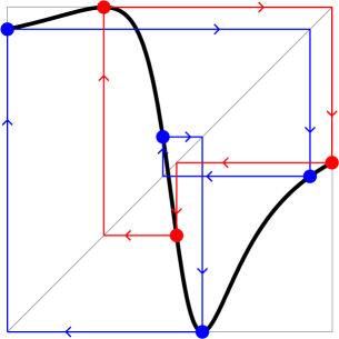
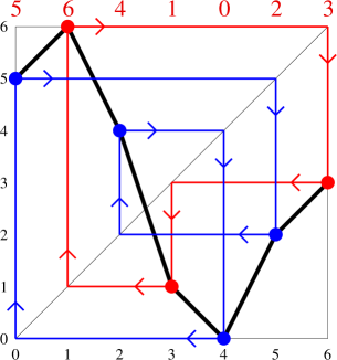
Figure 1: On the left a quadratic rational map with combinatorics ${(\!(}5,\,6,\,4,\,1,\,0,\,2,\,3{)\!)}$, and with critical orbits of period three and four. On the right, the corresponding piecewise linear model, with the combinatorics shown along the top.

Of course any list of $n+1$ numbers between zero and $n$ will yield a corresponding piecewise linear graph; but most such graphs could not possibly represent a quadratic map. In Section 2 we will specify strong and explicit restrictions on which lists ${\stackrel{{\scriptstyle\rightarrow}}{{m}}}$ are to be considered.

1. If there is only one critical point in $f({\widehat{\mathbb{R}}})$, then it might seem that it doesn’t matter whether the other critical point is to the left or the right of $f({\widehat{\mathbb{R}}})$ or at infinity, since we can always change this by replacing $f$ by a conjugate map. However, the following explicit choice of where to put it in the combinatorics will be important later:

   If one critical point is outside of $f({\widehat{\mathbb{R}}})$ then put it:

   • to the left in the combinatorics if the associated critical value is a maximum,

   • or to the right if it is a minimum.

   In the first case, the combinatorics will start with $m_{0}=n$, with all $m_{j}>0$. In the second case it will end with $m_{n}=0$, with all $m_{j}<n$. (Compare Figure 2.)

   Otherwise the definition proceeds just as above.

  

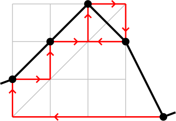
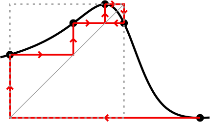
Figure 2: Graphs of the piecewise linear model map with combinatorics ${(\!(}1,\,2,\,3,\,2,\,0{)\!)}$, and the associated rational map. The mapping pattern is $\underline{\underline{x_{4}}}\mapsto x_{0}\mapsto x_{1}\mapsto\underline{\underline{x_{2}}}\leftrightarrow x_{3}$ (with the critical points double underlined). The square $[0,3]\times[0,3]$ on the left, with gray grid lines, corresponds to the square $f({\widehat{\mathbb{R}}})\times f({\widehat{\mathbb{R}}})$, outlined by dotted lines on the right. In this example, since the fixed point must lie between the two critical points, the critical point which is outside $f({\widehat{\mathbb{R}}})$ must be placed to the right.

Remark (Mapping Patterns).

By an abstract mapping pattern we will mean simply a finite set $S$ of marked points, together with a function from $S$ to itself, and a two element subset $S_{0}\subset S$ consisting of “critical points”. Evidently our combinatorics is essentially just a special kind of mapping pattern, together with an explicit ordering of the points of $S$. Given such an abstract mapping pattern, there may be several compatible combinatorics, or there may be none.

Now suppose that $S$ is given as a subset of ${\widehat{\mathbb{R}}}$. Then at least we are given a cyclic order of the points of $S$.

Lemma .

Given such an abstract mapping pattern, together with a cyclic ordering of $S$, there is at most one compatible combinatorics.

Proof.

In fact we can easily find the corresponding combinatorics (if it exists), in two steps as follows.

1. List these marked points in positive cyclic order; for example as

   $$x_{0}~{}<~{}x_{1}~{}<~{}\cdots~{}<~{}x_{n}~{},$$

   where all of the entries except possibly the last are finite.

Then one of the following should be true: Either the two critical values are next to each other in cyclic order; or they are separated in cyclic order only by a single critical point. (If neither is true, then the mapping pattern is not compatible with any real quadratic map.)

1. Assuming that this is the case, there is a unique cyclic permutation $x^{\prime}_{0},~{}x^{\prime}_{1},~{}\cdots,~{}x^{\prime}_{n}$ of the $x_{j}$ so that either:

   • the two extreme points $x^{\prime}_{0}$ and $x^{\prime}_{n}$ are the two critical values; or

   • the two extreme points are a critical point and its associated critical value, with the other critical value next to this critical point.

The required combinatorics ${\stackrel{{\scriptstyle\rightarrow}}{{m}}}$ is then defined by the usual rule: $f(x^{\prime}_{j})=x^{\prime}_{m_{j}}$. ∎

If we started with a mapping pattern which is possible for a real quadratic map, then the resulting ${\stackrel{{\scriptstyle\rightarrow}}{{m}}}$ will always be admissible, as defined below.

Definition (Admissibility).

There are several restrictions that one can put of the sequence ${\stackrel{{\scriptstyle\rightarrow}}{{m}}}$ of $n+1$ integers between zero and $n$. We will say that ${\stackrel{{\scriptstyle\rightarrow}}{{m}}}$ is admissible if it satisfies the following two essential conditions. (Four further possible restrictions will be described later.)

1. The difference between the largest $m_{j}$ and the smallest is either $n$ (in Case 1) or $n-1$ (in (2)). Furthermore, in (2), either the first entry will be $n$ or the last entry will be zero.

2. After a cyclic permutation which places the smallest $m_{j}$ on the left the resulting sequence will consist of a strictly monotone increasing sequence from smallest to largest, followed by a strictly decreasing sequence which never gets as far as the smallest.

As examples, for Figure 1 the cyclically permuted sequence would be

$$0,~{}2,~{}3,~{}5,~{}6,~{}4,~{}1~{}$$

while for Figure 2 it would be $0,~{}1,~{}2,~{}3,~{}2$. One immediate consequence of Condition (2) is that no $m_{j}$ can occur more than two times in the sequence. This is clearly a necessary property for quadratic maps.

To relate these properties to Thurston’s ideas, we need the following.

Definition .

A Thurston map is an orientation preserving branched covering map from a topological 2-sphere to itself such that the forward orbit of any branch point is finite.

The branch points are often referred to as “critical points” and their iterated forward images as “postcritical points”. See [KL] for a detailed classification of all Thurston maps with at most four postcritical points.

For our purposes, we can take the Riemann sphere as our 2-sphere, and call a Thurston map real if it commutes with complex conjugation, and has real critical points.

Lemma .

Any admissible combinatorics gives rise to a real Thurston map of degree two.

Proof.

We will identify ${\widehat{\mathbb{R}}}$ with the equator $E$ of the Riemann sphere, which divides the sphere into a “northern hemisphere” and a “southern hemisphere”. (Compare Figure 3.) The pure imaginary complex numbers correspond to an orthogonal great circle $C$, which divides the sphere into an “eastern hemisphere” to the right, and a “western hemisphere” to the left. Each of these great circles is divided into a positive and negative semicircle; and they divide the sphere into four quadrants, which are labeled as 1 (for northeast) through 4 (for southeast).

Figure 3: The Riemann sphere, divided into four quadrants.

To begin the construction, place the marked points $x_{0}$ through $x_{n}$ in positive cyclic order around the equator in such a way that points in an increasing lap are placed in $E+$, those in a decreasing lap are placed in $E-$, while the two critical points are placed at the two points of $E\cap C$. Then choose a map ${\bf f}$ from $E$ to itself which sends each $x_{j}$ to $x_{m_{j}}$, and maps $E+$ by an orientation preserving homeomorphism, and $E-$ by an orientation reversing homeomorphism. Thus $E$ will be mapped two-to-one onto the set ${\bf f}({\widehat{\mathbb{R}}})\subset{\widehat{\mathbb{R}}}=E$. Now extend to a map from $E\cup C$ onto $E$ which sends each of the two semicircles $C\pm$ homeomorphically onto the closure of the gap ${\widehat{\mathbb{R}}}{\smallsetminus}{\bf f}({\widehat{\mathbb{R}}})$.

Then it is not hard to check that the boundary of each of the four quadrants maps homeomorphically onto the equator. It follows that we can extend to a map ${\bf f}$ from the Riemann sphere onto itself which sends the first and third quadrants homeomorphically onto the northern hemisphere, and sends the second and fourth quadrants homeomorphically onto the southern hemisphere. This is the required two-fold branched covering map, branched only at the two points of $E\cap C$.∎

We will say that the combinatorics ${\stackrel{{\scriptstyle\rightarrow}}{{m}}}$ is unobstructed if there exists a rational map having combinatorics ${\stackrel{{\scriptstyle\rightarrow}}{{m}}}$. Otherwise it is obstructed. In nearly every case, if the combinatorics is unobstructed, then Thurston’s iterated pull-back construction, as described in §4, converges locally uniformly to the required rational map. (Compare §5.) For the unique exceptional case, see Section 5.

In addition to the essential requirements (1) and (2) described earlier, there are four further requirements that we may want to impose on the combinatorics. We will refer to $\{0,\,1,\,\cdots,\,n\}$ as the “marked points” for the associated piecewise linear map, and the two points where this map is maximized or minimized as the “critical points”.

We will say that the combinatorics is minimal if it is admissible, and also satisfies the following two conditions, which say roughly that every vertex and every edge of the associated PL graph is essential.

1. (All marked points are critical or postcritical) (Compare Figure 4.) Of course this condition is automatically satisfied for combinatorics constructed from a given postcritically finite map, as described in the beginning of this section.

2. (Expansiveness) For any edge of the piecewise linear model, some forward image contains a critical point. (Compare Figure 5.)

For the analogous theory for polynomial maps of any degree, there is no Thurston obstruction if and only if the corresponding condition is satisfied. (Compare [BS] and [P], as well as [BMS].) However for quadratic rational maps, although this is still a necessary condition, it is far from sufficient: In many cases, there is an obstruction even when the combinatorics is expansive.

Remark (Lifted Graphics).

From now on, most graphs of quadratic rational maps will be shown in lifted normal form. The precise definition will be given in Section 3; but roughly speaking this is a form which provides a uniform presentation in which the point at infinity does not play any special role. The parameters $\mu$ and $\kappa$ which uniquely determine the map will usually be given in LABEL:t-2 of Appendix B.

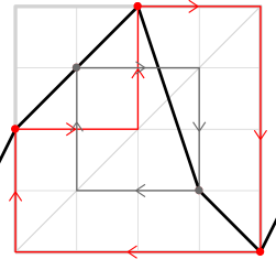
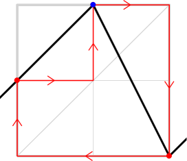
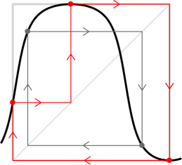
Figure 4: The combinatorics ${(\!(}2,\,3,\,4,\,1,\,0{)\!)}$ is not minimal, since the points $1$ and $3$ are not critical or postcritical. Removing $1$ and $3$ and renumbering, we get the simplified combinatorics ${(\!(}1,\,2,\,0{)\!)}$. The resulting rational map will be the same in either case. The only difference is that in the graph of the corresponding rational map, the period two orbit $x_{1}\leftrightarrow x_{3}$ will be shown in the first case but not in the second.

    

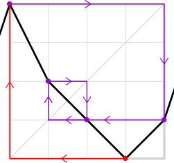
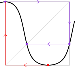
Figure 5: An example of combinatorics which satisfies Condition (3) but is not expansive. Here $n=4$, the map has combinatorics ${(\!(}4,\,2,\,1,\,0,\,1{)\!)}$. The edge $[2,\,3]$ is not expansive, and hence collapses to a point in the corresponding lifted rational map, which has simplified combinatorics ${(\!(}3,\,1,\,0,\,1{)\!)}$.

Remark .

In most cases, any admissible combinatorics which is not minimal can be reduced to a minimal example with simplified combinatorics in three steps as follows. (Compare Figures 4 and 5.) However this is not always possible, so a fourth step is needed.

1. Remove any vertices of the PL model which are not critical or postcritical.

2. Collapse any edge which is not expansive to a point.

3. Renumber the vertices which are left.

4. Check that the resulting combinatorics is admissible. (For an example where this last step fails, see Figure 6.)

    

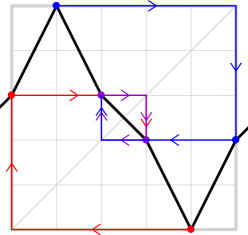
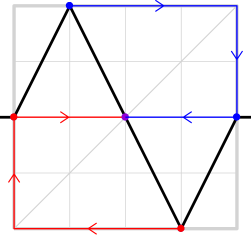
Figure 6: The combinatorics ${(\!(}3,\,5,\,3,\,2,\,0,\,2{)\!)}$ on the left is admissible, although not minimal. However, if we try to reduce it to a minimal example, we obtain the combinatorics ${(\!(}2,\,4,\,2,\,0,\,2{)\!)}$ on the right, which is not admissible and hence cannot describe any quadratic example, since one horizontal line intersects the graph three times. (In the terminology we will introduce in Section 7, it follows that the combinatorics on the left is “strongly obstructed”.)

There are two further restrictions which we may sometimes want to impose on the combinatorics.

1. (Not a polynomial). The combinatorics satisfies $m_{0}>0$ and $m_{n}<n$ so that there is no critical fixed point. There is nothing wrong with combinatorics with a critical fixed point since they correspond to maps conjugate to a polynomial. In fact they are much easier to deal with; and quadratic polynomials are well understood. However, we will concentrate on non-polynomial maps in the subsequent discussion, except in Section 8 where polynomial maps will play an essential role).

Figure 7: A piecewise linear example with combinatorics ${(\!(}1,\,0,\,3,\,2{)\!)}$ and with three fixed points. See also Figure 46R.

1. (Only one fixed point) The associated piecewise linear model has exactly one fixed point. This is closely related to the previous requirement, since a critically finite quadratic polynomial always has three fixed points. However we will see in Section 3 that a critically finite quadratic map which is not conjugate to a polynomial always has just one fixed point. Thus for combinatorics such as ${(\!(}1,~{}0,~{}3,~{}2{)\!)}$, as illustrated in Figure 7, there must be a Thurston obstruction. (Compare Section 7 and [M, Lemma 10.2]. )

Remark (Dynamic Classification).

By definition a critically finite rational map is hyperbolic if every postcritical cycle contains at least one critical point. In the quadratic case, every hyperbolic map belongs to one of the following three types:

Type B (bicritical).

Both critical points are contained in a common periodic orbit. (Compare Figure 4.)

Type C (capture).

The orbit of one critical point lands, after one or more iterations, on a periodic orbit containing the other critical point. (Compare Figure 2.)

Type D (disjoint).

The orbits of the two critical points are periodic and disjoint. (Compare Figure 1.)

Similarly, each non-hyperbolic map belongs to one of two types:

Half-Hyperbolic.

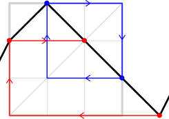
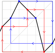
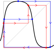
Figure 41: On the left: A strictly unimodal map of topological shape $+-$  and combinatorics ${(\!(}2,\,3,\,2,\,1,\,0{)\!)}$, with a periodic critical orbit $\underline{\underline{x_{1}}}\leftrightarrow x_{3}$ and an eventually repelling critical orbit $~{}\underline{\underline{x_{4}}}\mapsto x_{0}\mapsto x_{2}\,\rotatebox[origin={c}]{90.0}{\large$\circlearrowleft$}\,$. Here one critical point lies outside of $f({\widehat{\mathbb{R}}})$. On the right: topological shape $+-+$ and combinatorics ${(\!(}3,\,4,\,6,\,5,\,4,\,0,\,1{)\!)}$, with periodic orbit $\underline{\underline{x_{5}}}\mapsto x_{0}\mapsto x_{3}\mapsto\underline{\underline{x_{5}}}$ and repelling critical orbit $\underline{\underline{x_{2}}}\mapsto x_{6}\mapsto x_{1}\mapsto x_{4}\,\rotatebox[origin={c}]{90.0}{\large$\circlearrowleft$}\,$. Note that both critical points lie in $f({\widehat{\mathbb{R}}})$.

One critical orbit is periodic; but the other is only eventually periodic. (Compare Figure 41.)

Totally Non-Hyperbolic.

No critical orbit is periodic, although both are eventually periodic. (Compare Figure 42.)

Conjugacy classes of Hyperbolic Type are always isolated, since they are contained in an open hyperbolic component which contains no other critically finite point. However a sequence of hyperbolic critically finite conjugacy classes may well converge to a limit which is Half-Hyperbolic or Totally Non-Hyperbolic.

This classification extends easily to our piecewise-linear model maps, and hence to any admissible combinatorics.

Remark .

One important number associated with any combinatorics is the number of postcritical points, which we will denote by ${N_{\bf pc}}$. Note that ${N_{\bf pc}}=n+1$ for combinatorics of Type B or D, but ${N_{\bf pc}}=n$ in the Type C or Half-Hyperbolic cases; while ${N_{\bf pc}}$ may be either $n$ or $n-1$ in the Totally Non-Hyperbolic case. Cases with ${N_{\bf pc}}\leq 4$ require special attention in Thurston’s theory (Compare Section 5.)

Remark (Topological Classification).

Real quadratic maps can be classified topologically by the location of their critical points with respect to the interval $f({\widehat{\mathbb{R}}})$. For a very rough classification, let $\ell$ be the number of critical points in the interior of $f({\widehat{\mathbb{R}}})$. Then the map $f$ restricted to $f({\widehat{\mathbb{R}}})$ can be described as bimodal if $\ell=2$, or unimodal if $\ell=1$, and monotone if $\ell=0$.

The $\ell$ critical points divide $f({\widehat{\mathbb{R}}})$ into $\ell+1$ laps, or maximal intervals of monotonicity. On each lap, $f$ is either monotone increasing if $f^{\prime}>0$ (indicated by a plus sign), or monotone decreasing if $f^{\prime}<0$ (indicated by a minus). Thus in the bimodal case we either have the case $+-+$ or the case $-+-$, with a similar dichotomy for the unimodal and monotone cases.

$\displaystyle+\,-\,+$	$\displaystyle+\,-$	$\displaystyle+$
$\displaystyle-\,+\,-$	$\displaystyle-\,+$	$\displaystyle-$

Figure 8: The six possible shapes for maps which have no critical point on the boundary of $f({\widehat{\mathbb{R}}})$. The left two figures are of bimodal shape, the middle two of unimodal shape, and the last two of monotone shape. (The $+-$ and $-+$ cases are not really different from each other, since one can be obtained from the other by the orientation reversing change of coordinate $x\leftrightarrow 1-x$.)

For a more precise classification, we must single out the cases where there is a critical point precisely in the boundary of $f({\widehat{\mathbb{R}}})$, or in other words, a critical point which is also a critical value. There are two possibilities:

Definition .

The quadratic map $f$ is of polynomial shape if it has a critical fixed point; and is of co-polynomial shape if one critical point maps to the other. Note that $f$ is of polynomial shape if and only if it is conjugate to a polynomial; and is of co-polynomial shape if and only if it is conjugate to a map of the form $x\mapsto 1/p(x)$ where $p(x)$ is a polynomial. (See Section 8.)

We will say that a map is strictly unimodal if its restriction to $f({\widehat{\mathbb{R}}})$ is unimodal, and if there is no critical point of the boundary of $f({\widehat{\mathbb{R}}})$, so that it will remain unimodal under a small perturbation. Thus means that one critical point is in the interior and one critical point is strictly outside of $f({\widehat{\mathbb{R}}})$. Similarly it is strictly monotone if both critical points are strictly outside of $f({\widehat{\mathbb{R}}})$. (Compare Figure 8.)

This dynamic classification of maps gives rise to a corresponding partition of the “moduli space”, which consists of all conjugacy classes, into six connected open sets, and two connected closed sets made of points which are on the common boundary between two or more of these open sets. (Compare Figure 15 in Section 6.)

In the unimodal and bimodal cases, this classification extends easily to our PL model maps, and hence to any admissible combinatorics. However, there is no such thing as strictly monotone combinatorics.

Remark (Relations between dynamic and topological classifications).

Although these classifications are quite different, there are some obvious and some not so obvious relations between them. As an obvious relation, for combinatorics of Type B or D, both critical orbits are periodic, so we cannot be in the strictly unimodal case. Note also that co-polynomial combinatorics can only be of Type B, or Totally Non-Hyperbolic. This is true since any given point can have at most two immediate pre-images, counted with multiplicity. If for example the critical point $c_{1}$ maps to $c_{2}$, then no other point can map to $c_{2}$. Therefore we must be either in the Type B or the Totally Non-Hyperbolic case. A similar argument shows that polynomial combinatorics can only be of Type D or Half-Hyperbolic. Here is a less obvious example.

Proposition .

No combinatorics of shape $~{}-+-~{}$ can be of Type B.

Proof.

The piecewise linear map ${\bf f}:[0,n]\to[0,n]$ necessarily has three fixed points. Let $\widehat{x}$ be the middle fixed point. Then either $\widehat{x}>f(0)$ or $\widehat{x}<f(n)$ or both. In the first case the interval $[0,~{}\widehat{x}]$ maps to itself, and in the second case $[\widehat{x},~{}n]$ maps to itself. In either case, no periodic orbit can contain both zero and $n$. ∎

If we consider only unobstructed combinatorics, corresponding to actual quadratic maps, then there are further restrictions. We will see in Section 3 that the $(-+-)$-bimodal region does not contain any maps which are critically finite. However, it is easy to find combinatorics which are of shape $-+-$; and it follows that these must be strongly obstructed. See Appendix B for further information.

Remark (The Cross-Ratio Invariant).

One simple and useful invariant is the following. If $c_{1}$ and $c_{2}$ are the two critical points of $f$ and $v_{1}$, $v_{2}$ are the corresponding critical values, then the cross-ratio

$$\rho(f)~{}=~{}\frac{(c_{1}-v_{1})(c_{2}-v_{2})}{(c_{1}-c_{2})(v_{1}-v_{2}\ )}$$

is clearly invariant under fractional linear changes of coordinate. It is an easy exercise to check the following:

• $\rho=1$ if and only if $f$ is of polynomial shape.

• $\rho=0$ if and only if $f$ is of co-polynomial shape.

• $0<\rho<1$ if and only if $f$ is strictly unimodal.

• $\rho$ is finite in all cases.

However this invariant does not distinguish between the $+-+$ bimodal case and the $-$ monotone case, both with $\rho<0$. Similarly it does not distinguish between the $-+-$ bimodal case and the $+$ monotone case, both with $\rho>1$.

Remark (Orientation Reversal).

If we reverse orientation, then any given combinatorics ${\stackrel{{\scriptstyle\rightarrow}}{{m}}}={(\!(}m_{0},~{}\ldots,~{}m_{n}{)\!)}$ will be replaced by

$${\mathcal{I}}({\stackrel{{\scriptstyle\rightarrow}}{{m}}})~{}=~{}{(\!(}n-m_{n},~{}n-m_{n-1},~{}\ldots,~{}n-m_{1},~{}n-m_{0}{)\!)}~{}.$$

This corresponds to 180 degree rotation of the graph. It does not affect the dynamical classification or the cross-ratio invariant. However, it replaces any unimodal combinatorics of shape $+-$ by unimodal combinatorics of shape $-+$ with identical dynamic properties. For more on this orientation reversing involution, see Section 6 and Figure 17.

3 The Lifted Normal Form

The object of this section will be to introduce a family of real quadratic maps, parametrized by their two critical values, in a form which is easy to understand and which is convenient for carrying out the Thurston algorithm. The following will help to motivate the construction.

Lemma .

Let $f$ be a real quadratic map, not of polynomial shape, such that every real fixed point is strictly repelling. Then $f$ has precisely one real fixed point, and precisely one decreasing lap, which must contain this fixed point. Furthermore, there must be at least one critical point in $f({\widehat{\mathbb{R}}})$.

In particular, these statements apply to any critically finite map which is not of polynomial shape. For such maps, the unique real fixed point is always repelling, with multiplier ${\mu}<-1$. The map may be of shape $+-+$, or strictly unimodal, or co-polynomial; but it can never be of shape $-+-$, or strictly monotone. (These statements do not apply to critically finite maps of polynomial shape; so these may require slightly different treatment.)

Proof of Section 3.

First note every decreasing lap must contain exactly one fixed point. In fact, for the graph of the given lap, the left hand endpoint must be above the diagonal and the right hand endpoint must be below the diagonal; and it is easy to see that the graph cannot cross the diagonal twice. On the other hand, for an increasing lap there can be at most one fixed point. In fact the orbit of any point between two consecutive fixed points must converge to one or the other, which would contradict our hypothesis that there is no attracting or indifferent fixed point.

If a real quadratic map has two real fixed points, then it must have three, counted with multiplicity. Since we have excluded indifferent fixed points, this means that there must be three distinct laps, each with its own repelling fixed point. This is perfectly possible for a smooth or piecewise linear map. (Compare Figure 7.) But it is not possible for a quadratic map. According to [M], the multipliers of these three fixed points must be related by the equation

$${\mu}_{3}~{}=~{}\frac{2-{\mu}_{1}-{\mu}_{2}}{1-{\mu}_{1}{\mu}_{2}}~{}.$$

Thus if ${\mu}_{1}>1$ and ${\mu}_{2}>1$, then it follows that ${\mu}_{3}>0$; while if ${\mu}_{1}<-1$ and ${\mu}_{2}<-1$, it follows that ${\mu}_{3}<0$. Thus all three multipliers must have the same sign, which is impossible, since the sign must be positive in an increasing lap and negative in a decreasing lap. This contradiction proves that there can be only one fixed point; and hence only one decreasing lap. Finally note that every strictly monotone map must have an attracting or parabolic fixed point. In fact $f\circ f$ will always be monotone increasing on $f({\widehat{\mathbb{R}}})$, hence every orbit of $f\circ f$ must converge to an attracting or parabolic fixed point. ∎

In particular, it follows that a bimodal map of shape $~{}-+-~{}$ with two decreasing laps can never be critically finite. Furthermore, it is not hard to check that a map with only one lap is critically finite only in two very special cases, namely maps $\pm$-conjugate to $f(x)=x^{2}$ or $f(x)=1/x^{2}$.

We are finally ready to discuss normal forms. We will be primarily interested in maps which have exactly one fixed point in the lap between the two critical points. This will be called the primary fixed point. In such cases, the map is conjugate to a uniquely defined map with critical points at $\pm 1$ and with primary fixed point at zero. We can write the resulting map in Epstein normal form as

$$f(x)~{}=~{}\frac{{\mu}x}{x^{2}+2{\kappa}x+1}~{}.$$ (3.1)

(Compare Epstein [E], as well as DeMarco [D].) Note the identity $f(x)=f(1/x)$. Here $x=0$ is a fixed point of multiplier ${\mu}\neq 0~{}$. The critical points are $c_{1}=-1$ and $c_{2}=1$, and the associated critical values are

$$v_{1}=\frac{{\mu}}{2({\kappa}-1)}\quad{\rm and}\quad v_{2}=\frac{{\mu}}{2({\kappa}+1)}~{}.$$

Alternatively we can solve for the two parameters as functions of the critical values, with

$${\mu}=\frac{4v_{1}v_{2}}{v_{1}-v_{2}}\quad{\rm and}\quad{\kappa}=\frac{v_{1}+v_{2}}{v_{1}-v_{2}}~{}.$$ (3.2)

This may seem ideal for the Thurston algorithm. However in practice it seems to give very distorted pictures, and the poles at $x=-{\kappa}\pm\sqrt{{\kappa}^{2}-1}$ are awkward. Furthermore, there can be a drastic transition if we deform the parameters. If ${\kappa}$ passes through $\pm 1$, one critical value will pass through the point at infinity, and two poles will appear or disappear. In fact for any normal form that we choose, it may seem that the infinite point will cause trouble for some maps of interest.

However there is an easy way to avoid this problem. The space ${\widehat{\mathbb{R}}}\cong{\mathbb{P}}^{1}({\mathbb{R}})$ can be identified with the quotient ${\mathbb{R}}/{\mathbb{Z}}$, identifying each $t\in{\mathbb{R}}/{\mathbb{Z}}$ with $\tan(\pi t)\in{\widehat{\mathbb{R}}}$, or with $\big{(}\sin(\pi t):\cos(\pi t)\big{)}$ in the real projective line. Hence the universal covering space of ${\widehat{\mathbb{R}}}$ can be identified with the real line. Any real quadratic map $f:{\widehat{\mathbb{R}}}\to{\widehat{\mathbb{R}}}$ (always of degree zero) lifts to a periodic map ${\widetilde{f}}:{\mathbb{R}}\to{\mathbb{R}}$ with ${\widetilde{f}}(t+1)={\widetilde{f}}(t)$. Furthermore, $f$ restricted to a neighborhood of $f({\widehat{\mathbb{R}}})$ is real analytically conjugate to ${\widetilde{f}}$ restricted to a corresponding neighborhood of ${\widetilde{f}}({\mathbb{R}})$.

Another way of thinking of this is the following. Since the circle ${\widehat{\mathbb{R}}}$ is canonically isomorphic to ${\mathbb{R}}/{\mathbb{Z}}$, the graph of $f$ can be thought of as a subset of the torus $({\mathbb{R}}/{\mathbb{Z}})\times({\mathbb{R}}/{\mathbb{Z}})$. This torus is conveniently represented by a square $[0,1]\times[0,1]$ with opposite edges identified. Compare Figure 9 (where the coordinate of ${\mathbb{R}}$ has been translated so that ${\widetilde{f}}({\mathbb{R}})\subset[0,1]$).

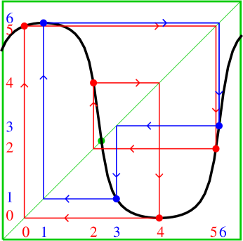
Figure 9: The Wittner map of Figure 1, lifted to the universal covering space of ${\widehat{\mathbb{R}}}$. Here the heavy green lines bound a fundamental domain. Thus the corresponding graph in the torus ${\widehat{\mathbb{R}}}\times{\widehat{\mathbb{R}}}$ can be obtained from this picture simply by identifying opposite green edges. Note that the product $f({\widehat{\mathbb{R}}})\times f({\widehat{\mathbb{R}}})$ corresponds to a square which is properly contained in this fundamental domain.

Thus if we use the Epstein normal form lifted to the universal covering space, then we will have a unique normal form such that the graph will deform smoothly as we change the parameters. Note that the fixed point is half way between the two critical points, either in Epstein normal form or in lifted form.

Lemma .

For the map $f$ of Equation (missing) 3.1, the corresponding lifted map $F$ is given by

$$t\mapsto F(t)~{}=~{}\frac{1}{\pi}\operatorname{Arg\,}(z)~{},$$

where $z=(1+\kappa\sin(2\pi t))+i(\mu\sin(2\pi t)/2)\,\in\,{\mathbb{C}}$, and $\operatorname{Arg\,}(z)$ is the branch of the argument with $-\pi<\operatorname{Arg\,}(z)<\pi$ .

Proof.

Let $x=\sin(\pi t)/\cos(\pi t)\in{\widehat{\mathbb{R}}}$ with $t\in{\mathbb{R}}/{\mathbb{Z}}$. After replacing $x$ in Equation (missing) 3.1, a brief computation shows that,

$$f(x)~{}=~{}\frac{\mu\sin(2\pi t)/2}{1+\kappa\sin(2\pi t)}~{}.$$ (3.3)

Notice that the right hand side of (3.3) is the slope of the line from $0$ to $z$ in ${\mathbb{C}}$. ∎

Remark .

There seems to be a problem since the function $z\mapsto\operatorname{Arg\,}(z)$ has a jump discontinuity on the negative real axis. However $z$ is never negative real, since $\mu\neq 0$ and since if $\sin(2\pi t)=0$ then $z=1$.

The lifted map of Section 3 will be used in the implementation of the algorithm described in the next section.

As an example, putting the Wittner map of Figure 1 into lifted normal form we obtain Figure 9. As another example, Figure 10 shows the lifted normal form for the map

$$f(x)~{}=~{}\frac{x^{2}-1}{x^{2}+1}~{}.$$

In this case we have $x_{0}=\infty,~{}x_{1}=-1,~{}x_{2}=0$, and $x_{3}=1$, with combinatorics ${(\!(}3,\,2,\,1,\,2{)\!)}$. The mapping pattern is

$$\lx@xy@svg{\hbox{\raise 0.0pt\hbox{\kern 5.5pt\hbox{\ignorespaces\ignorespaces\ignorespaces\hbox{\vtop{\kern 0.0pt\offinterlineskip\halign{\entry@#!@&&\entry@@#!@\cr&&&\crcr}}}\ignorespaces{\hbox{\kern-5.5pt\raise 0.0pt\hbox{\hbox{\kern 0.0pt\raise 0.0pt\hbox{\hbox{\kern 3.0pt\raise 0.0pt\hbox{$\textstyle{\underline{\underline{x_{0}}}\ignorespaces\ignorespaces\ignorespaces\ignorespaces}$}}}}}}}\ignorespaces\ignorespaces\ignorespaces\ignorespaces{\hbox{\kern 5.50002pt\raise 0.0pt\hbox{\hbox{\kern 0.0pt\raise 0.0pt\hbox{\lx@xy@stopper}}}}}{\hbox{\lx@xy@droprule}}\ignorespaces{\hbox{\kern 29.5pt\raise 0.0pt\hbox{\hbox{\kern 0.0pt\raise 0.0pt\hbox{\lx@xy@tip{1}\lx@xy@tip{-1}}}}}}{\hbox{\lx@xy@droprule}}{\hbox{\lx@xy@droprule}}{\hbox{\kern 29.5pt\raise 0.0pt\hbox{\hbox{\kern 0.0pt\raise 0.0pt\hbox{\hbox{\kern 3.0pt\raise 0.0pt\hbox{$\textstyle{x_{3}\ignorespaces\ignorespaces\ignorespaces\ignorespaces}$}}}}}}}\ignorespaces\ignorespaces\ignorespaces\ignorespaces{\hbox{\kern 44.01527pt\raise 0.0pt\hbox{\hbox{\kern 0.0pt\raise 0.0pt\hbox{\lx@xy@stopper}}}}}{\hbox{\lx@xy@droprule}}\ignorespaces{\hbox{\kern 68.01526pt\raise 0.0pt\hbox{\hbox{\kern 0.0pt\raise 0.0pt\hbox{\lx@xy@tip{1}\lx@xy@tip{-1}}}}}}{\hbox{\lx@xy@droprule}}{\hbox{\lx@xy@droprule}}{\hbox{\kern 68.01526pt\raise 0.0pt\hbox{\hbox{\kern 0.0pt\raise 0.0pt\hbox{\hbox{\kern 3.0pt\raise 0.0pt\hbox{$\textstyle{\underline{\underline{x_{2}}}\ignorespaces\ignorespaces\ignorespaces\ignorespaces}$}}}}}}}\ignorespaces\ignorespaces\ignorespaces\ignorespaces{\hbox{\kern 79.01527pt\raise 0.0pt\hbox{\hbox{\kern 0.0pt\raise 0.0pt\hbox{\lx@xy@tip{1}\lx@xy@tip{-1}}}}}}{\hbox{\lx@xy@droprule}}\ignorespaces{\hbox{\kern 103.01526pt\raise 0.0pt\hbox{\hbox{\kern 0.0pt\raise 0.0pt\hbox{\lx@xy@tip{1}\lx@xy@tip{-1}}}}}}{\hbox{\lx@xy@droprule}}{\hbox{\lx@xy@droprule}}{\hbox{\kern 103.01526pt\raise 0.0pt\hbox{\hbox{\kern 0.0pt\raise 0.0pt\hbox{\hbox{\kern 3.0pt\raise 0.0pt\hbox{$\textstyle{x_{1}~{}}$}}}}}}}\ignorespaces}}}}\ignorespaces. \textstyle{\underline{\underline{x_{0}}}\ignorespaces\ignorespaces\ignorespaces\ignorespaces} \textstyle{x_{3}\ignorespaces\ignorespaces\ignorespaces\ignorespaces} \textstyle{\underline{\underline{x_{2}}}\ignorespaces\ignorespaces\ignorespaces\ignorespaces} \textstyle{x_{1}~{}} \textstyle{\underline{\underline{x_{0}}}\ignorespaces\ignorespaces\ignorespaces\ignorespaces} \textstyle{x_{3}\ignorespaces\ignorespaces\ignorespaces\ignorespaces} \textstyle{\underline{\underline{x_{2}}}\ignorespaces\ignorespaces\ignorespaces\ignorespaces} \textstyle{x_{1}~{}}$$

  

Figure 10: The map $x\mapsto(x^{2}-1)/(x^{2}+1)$. On the left is shown the rational map for $-2.5<x<2.5$ along with the forward orbits of the critical points $\infty$ (blue) and $0$ (red). On the right is shown the map lifted to the universal covering line. In both cases, $f({\widehat{\mathbb{R}}})\times f({\widehat{\mathbb{R}}})$ is shown as a gray box. Note that the critical point $x_{0}$ is not within $f({\widehat{\mathbb{R}}})$.

4 The Algorithm

For any real quadratic map, the circle ${\widehat{\mathbb{R}}}$ is divided by the two real critical points into an “increasing” (or orientation preserving) half-circle and a “decreasing” half-circle. For $x$ in the interior of $f({\widehat{\mathbb{R}}})$, there is one branch $f_{+}^{-1}$ of $f^{-1}$ taking values in the increasing half-circle, and one branch $f_{-}^{-1}$ taking values in the decreasing half-circle. Note that these two branches of $f^{-1}$ coincide at the critical values, which map to critical points.

Suppose that some admissible combinatorics ${\stackrel{{\scriptstyle\rightarrow}}{{m}}}$ has been specified (see Section 2). Let $m_{j_{1}}$ be the smallest $m_{j}$ and let $m_{j_{2}}$ be the largest one. The two “critical” indices $j_{1}$ and $j_{2}$ divide $\{0,\ldots,n\}$ into two or three laps, each of which is either increasing or decreasing. We will always assume that $n\geq 2$.

The basic construction.

Let $X_{n}\subset{\widehat{\mathbb{R}}}^{n+1}$ be the space consisting of all $(n+1)$-tuples ${\stackrel{{\scriptstyle\rightarrow}}{{x}}}=(x_{0},\cdots,x_{n})$ of distinct points of ${\widehat{\mathbb{R}}}$ which are in positive cyclic order. Let $f$ be a quadratic rational map such that $f({\widehat{\mathbb{R}}})$ is precisely the smallest interval containing all of the $x_{m_{j}}$. In other words, $f({\widehat{\mathbb{R}}})$ is the interval consisting of all points $x$ which lie between the critical values $x_{m_{j_{1}}}$ and $x_{m_{j_{2}}}$ in cyclic order. Then the pullback $T_{f}({\stackrel{{\scriptstyle\rightarrow}}{{x}}})={\stackrel{{\scriptstyle\rightarrow}}{{y}}}$ is defined by setting

$$y_{j}~{}=~{}f_{\pm}^{-1}(x_{m_{j}})~{},$$

using either $f_{+}^{-1}$ or $f_{-}^{-1}$ according as $m_{j}$ is in an increasing or decreasing lap. (In the case where $j$ is critical index, it doesn’t matter which branch we choose.) It is not hard to check that the image points $y_{j}$ are always in positive cyclic order.

Theorem .

Every admissible combinatorics ${\stackrel{{\scriptstyle\rightarrow}}{{m}}}$ gives rise to a well defined pullback map $~{}~{}T:X_{n}/G\to X_{n}/G$.

Proof.

We will prove first that this construction does not depend on the choice of $f$. Any other quadratic rational map satisfying the same conditions can be written as a composition $f\circ L$ where $L$ belongs to the group $G={\rm PSL}_{2}({\mathbb{R}})$ of orientation preserving fractional linear transformations. Then $(f\circ L)^{-1}=L^{-1}\circ f^{-1}$, and it follows that ${\stackrel{{\scriptstyle\rightarrow}}{{y}}}$ will be replaced by $L^{-1}({\stackrel{{\scriptstyle\rightarrow}}{{y}}})$, using the diagonal action of $G$ on $X_{n}$.

On the other hand, if we replace each ${\stackrel{{\scriptstyle\rightarrow}}{{x}}}$ by $L({\stackrel{{\scriptstyle\rightarrow}}{{x}}})$, then the image ${\stackrel{{\scriptstyle\rightarrow}}{{y}}}$ will not change. In fact, we can simply replace $f$ by $L\circ f$, so that $L\circ f$ will map ${\widehat{\mathbb{R}}}$ to $L\big{(}f({\widehat{\mathbb{R}}})\big{)}$. Thus each $y_{j}$ will be replaced by the appropriate branch of

$$x_{j}~{}\mapsto~{}(L\circ f)^{-1}\big{(}L(x_{j})\big{)}=f^{-1}(x_{j})~{},$$

which is just $y_{j}$ itself. ∎

Note that this quotient space $X_{n}/G$ is diffeomorphic to a convex open subset of ${\mathbb{R}}^{n-2}$. In fact for each $\vec{x}$, we can choose a uniquely defined group element $L$ so that $L({\stackrel{{\scriptstyle\rightarrow}}{{x}}})={\stackrel{{\scriptstyle\rightarrow}}{{y}}}$ satisfies $y_{n-2}=1,~{}y_{n-1}=\infty,$ and $y_{n}=0$. Then the remaining $y_{j}$ must satisfy

$$\quad 0<y_{0}<y_{1}<\cdots<y_{n-3}<1~{}.$$

Thus they form an interior point of one standard model for the $(n-2)$-simplex.

If there is no Thurston obstruction, then in nearly every case, the iterated pullback converges to a unique point of $X_{n}/G$, and this determines a unique conjugacy class of quadratic rational maps. In the exceptional case, it converges to a pair of points on the (non-compact) line of fixed points of $T\circ T$; see Section 5. In the obstructed case, the sequence of points $T^{\circ k}({\stackrel{{\scriptstyle\rightarrow}}{{x}}})$ always leaves every compact subset of $X_{n}/G$.

The Lifted Pullback Map.

Before we begin, we must choose a convenient family of quadratic rational maps. As a consequence of Section 4, we can choose any convenient one, such as the Epstein normal form (see Equation (missing) 3.1), but nearly any such choice will leave us having to deal with infinity, even though all the interesting behavior occurs in a compact subset of ${\widehat{\mathbb{R}}}$. As noted in Section 3, it will be most convenient to lift to the universal covering space, that is, to work with the family

$$F(t)~{}=~{}F_{\mu,\kappa}(t)~{}=~{}\frac{1}{\pi}\operatorname{Arg\,}\Big{(}1+\kappa\,\sin(2\pi t)+i\,\mu\,\sin(2\pi t)/2\Big{)}$$ (4.1)

as in Section 3. This is a periodic function of period 1, with a fixed point of multiplier $F^{\prime}(0)=\mu\neq 0$ at $t=0$, with critical points at $t\equiv\pm 1/4~{}~{}({\rm mod}~{}{\mathbb{Z}})$, and with image $F({\mathbb{R}})\subset(-3/4,~{}3/4)$ bounded by the two critical values and of length strictly less than one. Note that $\mu$ and $\kappa$ can be determined uniquely from the critical values of $F$. If $F(-1/4)=v_{1}$ and $F(1/4)=v_{2}$, then by Equation (missing) 3.2:

$$\mu=\frac{4\tan(\pi v_{1})\,\tan(\pi v_{2})}{\tan(\pi v_{1})-\tan(\pi v_{2})}\quad\textrm{and}\quad\kappa=\frac{\tan(\pi v_{1})+\tan(\pi v_{2})}{\tan(\pi v_{1})-\tan(\pi v_{2})}\,.$$

Corollary .

For any admissible combinatorics ${\stackrel{{\scriptstyle\rightarrow}}{{m}}}$, there is a well-defined pullback map acting on elements of the lifted family $\eqref{E-LF}$.

Proof.

Given a map $F$ in the lifted family, we can obtain a map $f$ in Epstein form by conjugating with $t\mapsto x=\tan(\pi t)\in{\widehat{\mathbb{R}}}$, which is biholomorphic for $t$ in a complex neighborhood of $(-1,1)$. Hence the pullback acting on an element of the lifted family corresponds exactly to the pullback acting on $X_{n}/G$. ∎

Remark .

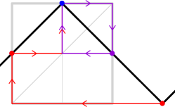
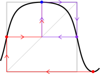
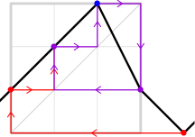
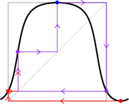
Figure 38: Strictly unimodal maps on $f({\widehat{\mathbb{R}}})$ of topological shape $+-$ . On the left are illustrations of a piecewise linear map and its corresponding rational map with $n=3$ and combinatorics ${(\!(}1,\,2,\,1,\,0{)\!)}$. This is a period 2 capture case with mapping pattern $\underline{\underline{x_{3}}}\mapsto x_{0}\mapsto\underline{\underline{x_{1}}}\leftrightarrow x_{2}$. On the right are illustrations of a map with $n=4$ and combinatorics ${(\!(}1,\,2,\,3,\,1,\,0{)\!)}$. This is capture with eventual period three. The mapping pattern is $\underline{\underline{x_{4}}}\mapsto x_{0}\rightarrow x_{1}\mapsto\underline{\underline{x_{2}}}\mapsto x_{3}\mapsto x_{1}$.

It is essential for our argument that the fixed point at $t=0$ must lie between the two critical points within the interval $f({\widehat{\mathbb{R}}})$. In the strictly unimodal case where there is only one critical point in $f({\widehat{\mathbb{R}}})$, the choice described in (2) of Section 2 is needed in order to ensure this property. As an explicit example, the map with combinatorics ${(\!(}1,2,1,0{)\!)}$ (see Figure 38-left) could also be described as the family with combinatorics ${(\!(}1,2,3,2{)\!)}$. However, this would not be consistent with our conventions in Section 2. The first has the mapping pattern $\underline{\underline{x_{3}}}\mapsto x_{0}\mapsto\underline{\underline{x_{1}}}\leftrightarrow x_{2}$, and the second $\underline{\underline{x_{0}}}\mapsto x_{1}\mapsto\underline{\underline{x_{2}}}\leftrightarrow x_{3}$. These are the same except for choice of labeling of the marked points. But the implicit ordering in the second does not follow our convention: both critical points are on the same side of the fixed point (which must lie between the points of the period 2 cycle $x_{2}\leftrightarrow x_{3}$). This would cause our implementation to fail.

Remark .

In our implementation, we only insist on the the first two admissibility conditions, and do not require those of minimality (3), expansiveness (4), non-polynomial (5), or unique fixed point (6).

However, for our implementation in the polynomial case, we will require the additional condition that the combinatorics must be of $+-$ shape, with a zero in the first entry. Thus: ${(\!(}0,\,2,\,1{)\!)}$ is the basilica, ${(\!(}0,\,3,\,4,\,5,\,6,\,2,\,1{)\!)}$ the period-doubled airplane, ${(\!(}0,\,1,\,3,\,1{)\!)}$ the Chebyshev point, and so on. Since $\mu$ is the value of the derivative at fixed point between the two critical points, the corresponding polynomial can be written as $\mu\,x(1-x)$. Of course polynomials can be dealt with by other methods. Compare [BMS]; and see Section 8 below.

Just as in Section 4, we will define the pullback $T=T_{F}$ as a map from a space of sequences to itself.

Definition .

Let $X({\stackrel{{\scriptstyle\rightarrow}}{{m}}})\subset{\mathbb{R}}^{n+1}$ be the space of all sequences ${\stackrel{{\scriptstyle\rightarrow}}{{t}}}=(t_{0},t_{1},\ldots,t_{n})$ which satisfy the following three conditions.

1. We must have

   $$-3/4~{}<~{}t_{0}~{}<~{}t_{1}~{}<~{}\cdots~{}<~{}t_{n}~{}<~{}3/4~{}.$$

2. If $j_{-}<j_{+}$ are the two critical indices, defined by the requirement that one of $m_{j_{-}}$ and $m_{j_{+}}$ is the largest $m_{j}$ and the other is the smallest, then

   $$t_{j_{-}}=-1/4\qquad{\rm and}\qquad t_{j_{+}}=+1/4~{}.$$

3. (Locating the fixed point.) If there is an index $j_{-}<p<j_{+}$ such that $m_{p}=p$, then we require that $t_{p}=0$. Otherwise there must be a unique pair of consecutive indices $j_{-}\leq p^{\prime}<p^{\prime\prime}\leq j_{+}$ such that the differences $m_{p^{\prime}}-p^{\prime}$ and $m_{p^{\prime\prime}}-p^{\prime\prime}$ have opposite sign. In this case, we require that

   $$t_{p^{\prime}}~{}<~{}0~{}<~{}t_{p^{\prime\prime}}~{}.$$

In order to define the pullback map $T({\stackrel{{\scriptstyle\rightarrow}}{{t}}})=\stackrel{{\scriptstyle\to}}{{t^{\prime}}}$, we must solve the equation $F(t^{\prime}_{j})=t_{m_{j}}$, taking care to choose between the two possible solutions. To do this, we divide the interval $[-3/4,\,3/4]$ into three subintervals:

$$I_{1}=(-3/4,\,-1/4),\quad I_{2}=(-1/4,\,1/4),~{}~{}{\rm and}\quad I_{3}=(1/4,\,3/4)~{}.$$ (4.2)

Here $I_{1}$ and $I_{3}$ are different lifts of the same half-circle, while $I_{2}$ corresponds to the other half-circle. Then the requirement is that $t_{j}$ and $t^{\prime}_{j}$ must belong to the same subinterval $I_{k}$. This is always uniquely possible since $F$ maps each interval $I_{k}$ bijectively onto the interval $F({\mathbb{R}})$.

Implementation.

We now give an outline of the steps involved in implementing the Thurston Algorithm. The implementation is very similar to that in [BMS]. When necessary, will use $t_{k}^{[\ell]}$ to denote the position of the $k$th marked point at the $\ell$th step, omitting this superscript when it is irrelevant or apparent. We will also use $F_{\ell}$ to indicate the map at the $\ell$th step, and $w_{k}^{[\ell]}$ for $F_{\ell}(t_{k}^{[\ell]})$.

Begin by examining the given combinatorics ${\stackrel{{\scriptstyle\rightarrow}}{{m}}}$, confirming admissibility and adherence to the requirements of Section 4. From the combinatorics, determine the indices of the critical points and the location of the fixed point lying between them, as described in Section 4. Finally, choose initial values of $t_{j}^{[0]}$ satisfying the required equalities and inequalities; and set $w_{j}^{[0]}=t_{m_{j}}^{[0]}$.

The inductive step in the construction can now be described as follows.

1. Increment $\ell$ by $1$, and determine $F_{\ell}$ from the critical values $w_{j_{\pm}}^{[\ell-1]}$.

2. For each $j$ other than the critical indices $j_{\pm}$ and or the fixed point index $p$ (when there is one), find the value of $t_{j}^{[\ell]}$ by numerically solving the equation $F_{\ell}(t^{[\ell]}_{j})=w^{[\ell-1]}_{j}$, with $t_{j}^{[\ell]}$ in the same interval $I_{k}$ as $t_{j}^{[\ell-1]}$.

3. If the results are close enough, then return $F_{\ell}$ and ${\stackrel{{\scriptstyle\rightarrow}}{{t}}}^{[\ell]}$. Otherwise, repeat the inductive step starting from (i).

Remark .

It might seem more natural to use the smaller intervals $I_{1}=(-\tfrac{1}{2},\,-\tfrac{1}{4})$ and $I_{3}=(\tfrac{1}{4},\,\tfrac{1}{2})$ in Equation (missing) 4.2. However, in some cases doing this leads to problems; and we found it more straightforward to just use the larger intervals.

In most cases, the calculations need to be done with at least double precision floating point arithmetic, and often require 20 or 30 decimal digits of working precision to get reasonably close to the limit.

We now explicitly discuss the pullback process for a specific example. Shown in Figure 11 are several steps for combinatorics ${(\!(}1,\,2,\,5,\,6,\,4,\,2,\,1,\,0{)\!)}$, with mapping pattern

This combinatorics is not minimal, since it includes the fixed point $t_{4}$, not part of any critical orbit. After omitting the fixed point and renumbering, we would obtain ${(\!(}1,\,2,\,4,\,5,\,2,\,1,\,0{)\!)}$.

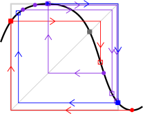
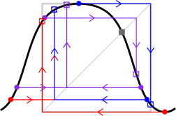
PL-model	step 0: $\mu\approx-2.168,\,\kappa\approx-.8778$	step 1: $\mu\approx-2.168,\,\kappa\approx-.8778$
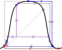
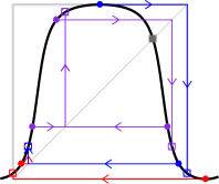
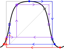
step 2: $\mu\approx-2.625,\,\kappa\approx-1.645$	step 3: $\mu\approx-3.255,\,\kappa\approx-1.649$	step 4: $\mu\approx-1.939,\,\kappa\approx-1.910$
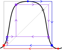
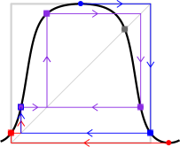
step 10: $\mu\approx-2.635,\,\kappa\approx-1.654$	step 20: $\mu\approx-2.592,\,\kappa\approx-1.637$	step 40: $\mu\approx-2.594,\,\kappa\approx-1.638$

Figure 11: The PL-model and several steps of the pullback process for the combinatorics ${(\!(}1,\,2,\,5,\,6,\,4,\,2,\,1,\,0{)\!)}$. Each of the marked points $t_{j}^{[\ell]}$ is indicated by a filled disk (either in blue, red, or purple) with attached arrows connecting to its image under $F_{\ell}$ (indicated by an open box). The critical point $t_{3}=-1/4$ and its forward images are drawn in blue, the critical point $t_{6}=1/4$ and its images are in red, and in purple are those which are a forward image of both critical points. The fixed point $t_{4}$ is in gray — it is not part of a critical orbit. (This convention will be used in most of the figures henceforth). Observe (in the bottom row) that by step 20, the graph has converged visually, but $\mu$ and $\kappa$ still change in the third decimal place.

In the set-up phase, we choose initial points $t_{0}^{[0]}$ through $t_{7}^{[0]}$, with $t_{3}=-1/4$, $t_{4}=0$, and $t_{7}=1/4$. The critical values $t_{0}$ and $t_{6}$ determine the map $F_{0}$ as in Equation (missing) 4.1. This is shown in Figure 11, top-center. Note that we have quite a lot of freedom in choosing the $t_{j}$, only subject to the restrictions of Section 4. In Figure 11, we have chosen the initial $t_{j}$ (other than the critical and fixed points) to be equally spaced within the intervals $(-1/2,-1/4)$ and $(0,1/4)$.

The values of $t_{j}^{[1]}$ are then computed by solving $F_{0}(t_{j}^{[1]})=t_{m_{j}}^{[0]}$. Since the map $F_{0}$ was determined by $t_{0}^{[0]}$ and $t_{6}^{[0]}$, we will have $F_{1}=F_{0}$, but the values of $t_{j}$ will change, in some cases dramatically.

We repeat the process again to obtain $F_{2}$ and $t_{j}^{[2]}$, and the dynamical behavior becomes roughly apparent (see the middle row of Figure 11), although none of the marked points actually map to each other. It takes 28 steps to get $\mu$ and $\kappa$ correct to three decimal places, and after 54 pullbacks $\mu$ and $\kappa$ are good to eight places.

5 The Unique Exceptional Case ${(\!(}1,\,3,\,4,\,3,\,1,\,0{)\!)}$

In this section we will prove the following.

Theorem .

Any critically finite real quadratic map $f$ is uniquely determined up to conjugacy by its combinatorics. In fact the conjugacy class $\langle f\rangle$ is the unique fixed point of the associated pull-back transformation. For any minimal combinatorics other than ${(\!(}1,\,3,\,4,\,3,\,1,\,0{)\!)}$ or its image under orientation reversal, this fixed point is a global attractor, so that the iterated pull-back transformation will always converge to a map in the required conjugacy class.

On the other hand:

Proposition .

In the exceptional case ${\stackrel{{\scriptstyle\rightarrow}}{{m}}}={(\!(}1,\,3,\,4,\,3,\,1,\,0{)\!)}$, the iterated pull-back $f\mapsto T(f)$ does not usually converge to a single map. Instead, from a generic starting point, it converges to a pair of maps $(f,g)$ for which $T(f)=g$ and $T(g)=f$. In fact the composition $T\circ T$ has a global attractor consisting of a one-parameter family of conjugacy classes, and the fixed point of $T$ is just one point in this one-parameter family.

    

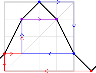
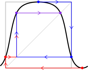
Figure 12: On the left, the PL model for combinatorics ${(\!(}1,\,3,\,4,\,3,\,1,\,0{)\!)}$. On the right is shown its realization in the lifted model, with $\mu=-2$ and $\kappa=-\sqrt{2}$. Note that the two critical values map to a common point, which maps to a fixed point.

Proof of Section 5.

Any quadratic map which has a non-critical fixed point can be put into the normal form

$$f_{v,w}(x)=\frac{(w-v)(x+x^{-1})}{4}+\frac{v+w}{2}~{}.$$ (5.1)

with critical points at $\pm 1$, fixed point at $\infty$, and critical values $~{}~{}f(1)=w\neq f(-1)=v$.In order for such a map to be compatible with the ${(\!(}1,3,4,3,1,0{)\!)}$ mapping pattern

$$\lx@xy@svg{\hbox{\raise 0.0pt\hbox{\kern 5.5pt\hbox{\ignorespaces\ignorespaces\ignorespaces\hbox{\vtop{\kern 0.0pt\offinterlineskip\halign{\entry@#!@&&\entry@@#!@\cr&&&&\\&&\crcr}}}\ignorespaces{\hbox{\kern-5.5pt\raise 0.0pt\hbox{\hbox{\kern 0.0pt\raise 0.0pt\hbox{\hbox{\kern 3.0pt\raise 0.0pt\hbox{$\textstyle{\underline{\underline{x_{2}}}\ignorespaces\ignorespaces\ignorespaces\ignorespaces}$}}}}}}}\ignorespaces\ignorespaces\ignorespaces\ignorespaces{\hbox{\kern 5.50002pt\raise 0.0pt\hbox{\hbox{\kern 0.0pt\raise 0.0pt\hbox{\lx@xy@stopper}}}}}{\hbox{\lx@xy@droprule}}\ignorespaces{\hbox{\kern 29.5pt\raise 0.0pt\hbox{\hbox{\kern 0.0pt\raise 0.0pt\hbox{\lx@xy@tip{1}\lx@xy@tip{-1}}}}}}{\hbox{\lx@xy@droprule}}{\hbox{\lx@xy@droprule}}{\hbox{\kern 29.5pt\raise 0.0pt\hbox{\hbox{\kern 0.0pt\raise 0.0pt\hbox{\hbox{\kern 3.0pt\raise 0.0pt\hbox{$\textstyle{x_{4}\ignorespaces\ignorespaces\ignorespaces\ignorespaces}$}}}}}}}\ignorespaces\ignorespaces\ignorespaces\ignorespaces{\hbox{\kern 44.01527pt\raise 0.0pt\hbox{\hbox{\kern 0.0pt\raise 0.0pt\hbox{\lx@xy@stopper}}}}}{\hbox{\lx@xy@droprule}}\ignorespaces{\hbox{\kern 68.01526pt\raise 0.0pt\hbox{\hbox{\kern 0.0pt\raise 0.0pt\hbox{\lx@xy@tip{1}\lx@xy@tip{-1}}}}}}{\hbox{\lx@xy@droprule}}{\hbox{\lx@xy@droprule}}{\hbox{\kern 68.01526pt\raise 0.0pt\hbox{\hbox{\kern 0.0pt\raise 0.0pt\hbox{\hbox{\kern 3.0pt\raise 0.0pt\hbox{$\textstyle{x_{1}\ignorespaces\ignorespaces\ignorespaces\ignorespaces}$}}}}}}}\ignorespaces\ignorespaces\ignorespaces\ignorespaces{}{\hbox{\lx@xy@droprule}}\ignorespaces{\hbox{\kern 75.27289pt\raise-14.10164pt\hbox{\hbox{\kern 0.0pt\raise 0.0pt\hbox{\lx@xy@tip{1}\lx@xy@tip{-1}}}}}}{\hbox{\lx@xy@droprule}}{\hbox{\lx@xy@droprule}}{\hbox{\kern 106.53052pt\raise 0.0pt\hbox{\hbox{\kern 0.0pt\raise 0.0pt\hbox{\hbox{\kern 3.0pt\raise 0.0pt\hbox{$\textstyle{x_{0}\ignorespaces\ignorespaces\ignorespaces\ignorespaces}$}}}}}}}\ignorespaces\ignorespaces\ignorespaces\ignorespaces{\hbox{\kern 106.53052pt\raise 0.0pt\hbox{\hbox{\kern 0.0pt\raise 0.0pt\hbox{\lx@xy@stopper}}}}}{\hbox{\lx@xy@droprule}}\ignorespaces{\hbox{\kern 82.53053pt\raise 0.0pt\hbox{\hbox{\kern 0.0pt\raise 0.0pt\hbox{\lx@xy@tip{1}\lx@xy@tip{-1}}}}}}{\hbox{\lx@xy@droprule}}{\hbox{\lx@xy@droprule}}{\hbox{\kern 145.04578pt\raise 0.0pt\hbox{\hbox{\kern 0.0pt\raise 0.0pt\hbox{\hbox{\kern 3.0pt\raise 0.0pt\hbox{$\textstyle{\underline{\underline{x_{5}}}\ignorespaces\ignorespaces\ignorespaces\ignorespaces}$}}}}}}}\ignorespaces\ignorespaces\ignorespaces\ignorespaces{\hbox{\kern 145.04578pt\raise 0.0pt\hbox{\hbox{\kern 0.0pt\raise 0.0pt\hbox{\lx@xy@stopper}}}}}{\hbox{\lx@xy@droprule}}\ignorespaces{\hbox{\kern 121.04579pt\raise 0.0pt\hbox{\hbox{\kern 0.0pt\raise 0.0pt\hbox{\lx@xy@tip{1}\lx@xy@tip{-1}}}}}}{\hbox{\lx@xy@droprule}}{\hbox{\lx@xy@droprule}}{\hbox{\kern-3.0pt\raise-21.40718pt\hbox{\hbox{\kern 0.0pt\raise 0.0pt\hbox{\hbox{\kern 3.0pt\raise 0.0pt\hbox{$\textstyle{}$}}}}}}}{\hbox{\kern 33.75763pt\raise-21.40718pt\hbox{\hbox{\kern 0.0pt\raise 0.0pt\hbox{\hbox{\kern 3.0pt\raise 0.0pt\hbox{$\textstyle{}$}}}}}}}{\hbox{\kern 68.01526pt\raise-21.40718pt\hbox{\hbox{\kern 0.0pt\raise 0.0pt\hbox{\hbox{\kern 3.0pt\raise 0.0pt\hbox{$\textstyle{x_{3}\ignorespaces\ignorespaces\ignorespaces\ignorespaces\ignorespaces\ignorespaces}$}}}}}}}\ignorespaces\ignorespaces\ignorespaces\ignorespaces\ignorespaces\ignorespaces\ignorespaces\ignorespaces\ignorespaces{}{}{}{}{{}{{}{{}{{}{{}}{}{{}}{}{{}{{}}{}{{}}{}{{}{{}}}}}}}}{}\ignorespaces\hbox{\hbox{\kern 0.0pt\raise 0.0pt\hbox{{}{}{{}}{{}{}{}{}}{}}}}\ignorespaces{}\ignorespaces{}{}{}{}{{}{{}}{}{{}}{}{{}}{}{{}{{}}{}{{}{{}}{}{{}}{}{{}{{}{{}{{}{{}}}}}}}}}{\hbox{\kern 81.0158pt\raise-26.2093pt\hbox{\hbox{\kern 0.0pt\raise 0.0pt\hbox{\lx@xy@tip{1}\lx@xy@tip{-1}}}}}}\ignorespaces\hbox{\hbox{\kern 0.0pt\raise 0.0pt\hbox{{}{}{}{{}}{{}{}{}{}\lx@xy@spline@}{}}}}\ignorespaces{}\ignorespaces\hbox{\hbox{\kern 0.0pt\raise 0.0pt\hbox{{}{}{{}}{{}{}{}{}}{}}}}\ignorespaces{}\ignorespaces}}}}\ignorespaces~{}~{}, \textstyle{\underline{\underline{x_{2}}}\ignorespaces\ignorespaces\ignorespaces\ignorespaces} \textstyle{x_{4}\ignorespaces\ignorespaces\ignorespaces\ignorespaces} \textstyle{x_{1}\ignorespaces\ignorespaces\ignorespaces\ignorespaces} \textstyle{x_{0}\ignorespaces\ignorespaces\ignorespaces\ignorespaces} \textstyle{\underline{\underline{x_{5}}}\ignorespaces\ignorespaces\ignorespaces\ignorespaces} \textstyle{x_{3}\ignorespaces\ignorespaces\ignorespaces\ignorespaces\ignorespaces\ignorespaces} \textstyle{\underline{\underline{x_{2}}}\ignorespaces\ignorespaces\ignorespaces\ignorespaces} \textstyle{x_{4}\ignorespaces\ignorespaces\ignorespaces\ignorespaces} \textstyle{x_{1}\ignorespaces\ignorespaces\ignorespaces\ignorespaces} \textstyle{x_{0}\ignorespaces\ignorespaces\ignorespaces\ignorespaces} \textstyle{\underline{\underline{x_{5}}}\ignorespaces\ignorespaces\ignorespaces\ignorespaces} \textstyle{x_{3}\ignorespaces\ignorespaces\ignorespaces\ignorespaces\ignorespaces\ignorespaces}$$

we must identify this with the pattern

$$\lx@xy@svg{\hbox{\raise 0.0pt\hbox{\kern 7.16496pt\hbox{\ignorespaces\ignorespaces\ignorespaces\hbox{\vtop{\kern 0.0pt\offinterlineskip\halign{\entry@#!@&&\entry@@#!@\cr&&&&\\&&\crcr}}}\ignorespaces{\hbox{\kern-7.16496pt\raise 0.0pt\hbox{\hbox{\kern 0.0pt\raise 0.0pt\hbox{\hbox{\kern 3.0pt\raise 0.0pt\hbox{$\textstyle{\underline{\underline{1}}~{}\ignorespaces\ignorespaces\ignorespaces\ignorespaces}$}}}}}}}\ignorespaces\ignorespaces\ignorespaces\ignorespaces{\hbox{\kern 7.16498pt\raise 0.0pt\hbox{\hbox{\kern 0.0pt\raise 0.0pt\hbox{\lx@xy@stopper}}}}}{\hbox{\lx@xy@droprule}}\ignorespaces{\hbox{\kern 31.16496pt\raise 0.0pt\hbox{\hbox{\kern 0.0pt\raise 0.0pt\hbox{\lx@xy@tip{1}\lx@xy@tip{-1}}}}}}{\hbox{\lx@xy@droprule}}{\hbox{\lx@xy@droprule}}{\hbox{\kern 31.16496pt\raise 0.0pt\hbox{\hbox{\kern 0.0pt\raise 0.0pt\hbox{\hbox{\kern 3.0pt\raise 0.0pt\hbox{$\textstyle{~{}w~{}\ignorespaces\ignorespaces\ignorespaces\ignorespaces}$}}}}}}}\ignorespaces\ignorespaces\ignorespaces\ignorespaces{\hbox{\kern 51.25307pt\raise 0.0pt\hbox{\hbox{\kern 0.0pt\raise 0.0pt\hbox{\lx@xy@stopper}}}}}{\hbox{\lx@xy@droprule}}\ignorespaces{\hbox{\kern 75.25307pt\raise 0.0pt\hbox{\hbox{\kern 0.0pt\raise 0.0pt\hbox{\lx@xy@tip{1}\lx@xy@tip{-1}}}}}}{\hbox{\lx@xy@droprule}}{\hbox{\lx@xy@droprule}}{\hbox{\kern 75.25307pt\raise 0.0pt\hbox{\hbox{\kern 0.0pt\raise 0.0pt\hbox{\hbox{\kern 3.0pt\raise 0.0pt\hbox{$\textstyle{~{}x_{1}~{}\ignorespaces\ignorespaces\ignorespaces\ignorespaces}$}}}}}}}\ignorespaces\ignorespaces\ignorespaces\ignorespaces{}{\hbox{\lx@xy@droprule}}\ignorespaces{\hbox{\kern 85.84062pt\raise-13.19942pt\hbox{\hbox{\kern 0.0pt\raise 0.0pt\hbox{\lx@xy@tip{1}\lx@xy@tip{-1}}}}}}{\hbox{\lx@xy@droprule}}{\hbox{\lx@xy@droprule}}{\hbox{\kern 120.42818pt\raise 0.0pt\hbox{\hbox{\kern 0.0pt\raise 0.0pt\hbox{\hbox{\kern 3.0pt\raise 0.0pt\hbox{$\textstyle{~{}v~{}\ignorespaces\ignorespaces\ignorespaces\ignorespaces}$}}}}}}}\ignorespaces\ignorespaces\ignorespaces\ignorespaces{\hbox{\kern 120.42818pt\raise 0.0pt\hbox{\hbox{\kern 0.0pt\raise 0.0pt\hbox{\lx@xy@stopper}}}}}{\hbox{\lx@xy@droprule}}\ignorespaces{\hbox{\kern 96.42819pt\raise 0.0pt\hbox{\hbox{\kern 0.0pt\raise 0.0pt\hbox{\lx@xy@tip{1}\lx@xy@tip{-1}}}}}}{\hbox{\lx@xy@droprule}}{\hbox{\lx@xy@droprule}}{\hbox{\kern 162.29402pt\raise 0.0pt\hbox{\hbox{\kern 0.0pt\raise 0.0pt\hbox{\hbox{\kern 3.0pt\raise 0.0pt\hbox{$\textstyle{~{}\underline{\underline{-1}}\ignorespaces\ignorespaces\ignorespaces\ignorespaces}$}}}}}}}\ignorespaces\ignorespaces\ignorespaces\ignorespaces{\hbox{\kern 162.29402pt\raise 0.0pt\hbox{\hbox{\kern 0.0pt\raise 0.0pt\hbox{\lx@xy@stopper}}}}}{\hbox{\lx@xy@droprule}}\ignorespaces{\hbox{\kern 138.29404pt\raise 0.0pt\hbox{\hbox{\kern 0.0pt\raise 0.0pt\hbox{\lx@xy@tip{1}\lx@xy@tip{-1}}}}}}{\hbox{\lx@xy@droprule}}{\hbox{\lx@xy@droprule}}{\hbox{\kern-3.0pt\raise-20.50496pt\hbox{\hbox{\kern 0.0pt\raise 0.0pt\hbox{\hbox{\kern 3.0pt\raise 0.0pt\hbox{$\textstyle{}$}}}}}}}{\hbox{\kern 38.20901pt\raise-20.50496pt\hbox{\hbox{\kern 0.0pt\raise 0.0pt\hbox{\hbox{\kern 3.0pt\raise 0.0pt\hbox{$\textstyle{}$}}}}}}}{\hbox{\kern 77.84062pt\raise-20.50496pt\hbox{\hbox{\kern 0.0pt\raise 0.0pt\hbox{\hbox{\kern 3.0pt\raise 0.0pt\hbox{$\textstyle{\infty\ignorespaces\ignorespaces\ignorespaces\ignorespaces\ignorespaces\ignorespaces}$}}}}}}}\ignorespaces\ignorespaces\ignorespaces\ignorespaces\ignorespaces\ignorespaces\ignorespaces\ignorespaces\ignorespaces{}{}{}{}{{}{{}{{}{{}{{}}{}{{}}{}{{}}{}{{}}{}{{}{{}{{}}{}{{}}{}{{}}}}}}}}{}\ignorespaces\hbox{\hbox{\kern 0.0pt\raise 0.0pt\hbox{{}{}{{}}{{}{}{}{}}{}}}}\ignorespaces{}\ignorespaces{}{}{}{}{{}{{}}{}{{}}{}{{}}{}{{}}{}{{}{{}}{}{{}{{}{{}{{}}{}{{}}{}{{}}}}}}}{\hbox{\kern 89.13412pt\raise-23.50095pt\hbox{\hbox{\kern 0.0pt\raise 0.0pt\hbox{\lx@xy@tip{1}\lx@xy@tip{-1}}}}}}\ignorespaces\hbox{\hbox{\kern 0.0pt\raise 0.0pt\hbox{{}{}{}{{}}{{}{}{}{}\lx@xy@spline@}{}}}}\ignorespaces{}\ignorespaces\hbox{\hbox{\kern 0.0pt\raise 0.0pt\hbox{{}{}{{}}{{}{}{}{}}{}}}}\ignorespaces{}\ignorespaces}}}}\ignorespaces~{}~{}. \textstyle{\underline{\underline{1}}~{}\ignorespaces\ignorespaces\ignorespaces\ignorespaces} \textstyle{~{}w~{}\ignorespaces\ignorespaces\ignorespaces\ignorespaces} \textstyle{~{}x_{1}~{}\ignorespaces\ignorespaces\ignorespaces\ignorespaces} \textstyle{~{}v~{}\ignorespaces\ignorespaces\ignorespaces\ignorespaces} \textstyle{~{}\underline{\underline{-1}}\ignorespaces\ignorespaces\ignorespaces\ignorespaces} \textstyle{\infty\ignorespaces\ignorespaces\ignorespaces\ignorespaces\ignorespaces\ignorespaces} \textstyle{\underline{\underline{1}}~{}\ignorespaces\ignorespaces\ignorespaces\ignorespaces} \textstyle{~{}w~{}\ignorespaces\ignorespaces\ignorespaces\ignorespaces} \textstyle{~{}x_{1}~{}\ignorespaces\ignorespaces\ignorespaces\ignorespaces} \textstyle{~{}v~{}\ignorespaces\ignorespaces\ignorespaces\ignorespaces} \textstyle{~{}\underline{\underline{-1}}\ignorespaces\ignorespaces\ignorespaces\ignorespaces} \textstyle{\infty\ignorespaces\ignorespaces\ignorespaces\ignorespaces\ignorespaces\ignorespaces}$$

In particular, we must assume that the points $(x_{0},x_{1},x_{2},x_{3},x_{4},x_{5})=(v,~{}x_{1},~{}1,~{}\infty,~{}w,-1)$ are in positive cyclic order, or in other words that

$$w~{}<~{}-1~{}<~{}v~{}<~{}x_{1}~{}<~{}1~{}.$$ (5.2)

Now suppose that we start with any map in the form (5.1) satisfying (5.2), and apply the ${(\!(}1,3,4,3,1,0{)\!)}$-pullback transformation. Then we obtain a new rational map $f$ for which the two critical values must map to a common point. Putting $f$ into the form (5.1) with the postcritical fixed point at infinity, the equation $f(v)=f(w)$ implies that $v+v^{-1}=w+w^{-1}$. Since $v$ can never be equal to $w$, this implies that $w=v^{-1}$. Similarly, since $x_{1}$ can never be equal to $\infty$, the equation $f(x_{1})=f(\infty)=\infty$ implies that $x_{1}=0$. In other words, as we iterate, after the first step we will always have a rational map of the form (5.1) with $w=v^{-1}$ and with $x_{1}=0$ More explicitly, we will show that the action of $T$ then corresponds to the transformation

$$(v,1/v)~{}\longleftrightarrow~{}(v^{\prime},1/v^{\prime})\qquad{\rm with}\qquad v^{\prime}=\frac{v+1}{v-1}~{}.$$

(See Figure 13 for an example with $v=-1/2\leftrightarrow v^{\prime}=-1/3$.)

  

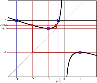
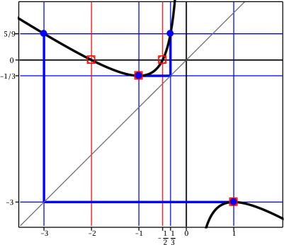
Figure 13: On the left is the rational map as in Equation (missing) 5.1 with critical values $v=-1/2$, $w=-2$ and on the right is its pullback with $v=-1/3$, $w=-3$. Conversely the left hand figure represents the pullback of the right hand one, so that this pair represents a two cycle for the pullback map. For each graph, the marked points are indicated by a solid disk (either in red or blue) with corresponding vertical and horizontal lines, and the pullbacks of these are also indicated with open boxes of the other color. Thus, in the left-hand figure, the points at $(-1/2,-5/16)$ and $(-2,-5/16)$ have only a red disk because they are marked points, but not the pullback of any marked point. By contrast, $(-1/3,0)$ and $(-3,0)$ are indicated by a blue square since these points are the pullback of $0$; the critical points at $x=\pm 1$ have both symbols, since they are both marked points and the pullback of a marked point.

Suppose that $(x_{0},\ldots,x_{5})$ are the marked points for $f=f_{v,w}$. To find the corresponding marked points $(x^{\prime}_{0},\ldots,x^{\prime}_{5})$ for the image under $T$ we must solve the equations

$$f(x^{\prime}_{j})~{}=~{}x_{m_{j}}~{},$$

taking care to choose the solution which belongs to the correct half-circles. In particular, to compute $v^{\prime}$ we must solve the quadratic equation $f(v^{\prime})=0$, choosing the solution which belongs to the lap $-1<v^{\prime}<0$. A brief computation shows that $v^{\prime}=(v+1)/(v-1)$ is the correct solution.

Since the fractional linear transformation $v\mapsto(v+1)/(v-1)$ has period two, it follows that $T\circ T$ is the identity for maps of this form. Furthermore, since the equation $v=v^{\prime}=(v+1)/(v-1)$ with $v<0$ implies that $v=1-\sqrt{2}$, it follows that $T$ has only one fixed point. This completes the proof of Section 5. ∎

Proof of Section 5.

To explain this behavior, we must go back to Douady and Hubbard. To every Thurston map (and therefore to every combinatorics), they assign an orbifold structure on the 2-sphere. It can be defined as follows (compare [DH, Page 2] ). Each point $x$ of the sphere is assigned a ramification index $\nu(x)\in\{1,2,3,\cdots,\infty\}$ which is greater than one if and only if $x$ is a postcritical point. More precisely, it can be defined as the supremum over all iterated preimages $f^{\circ k}(y)=x$ of the local degree of $f^{\circ k}$ at $y$. Thus $\nu(x)=\infty$ if and only if $x$ belongs to a periodic critical orbit; but $\nu(x)$ is bounded by the product of the local degrees of $f$ at its critical points otherwise. This orbifold structure has a well defined orbifold Euler characteristic $\chi\in{\mathbb{Q}}$ defined by the formula

$$\chi~{}=~{}2~{}-~{}\sum_{x}\Big{(}1-\frac{1}{\nu(x)}\Big{)}~{},$$ (5.3)

to be summed over all postcritical points. They show that $\chi\leq 0$ in all cases. By definition, the orbifold is Euclidean if $\chi=0$; and non-Euclidean if $\chi<0$. In particular, it is clearly non-Euclidean whenever the number of postcritical points satisfies ${N_{\bf pc}}>4$.

As an example, if $~{}~{}{\stackrel{{\scriptstyle\rightarrow}}{{m}}}={(\!(}1,\,3,\,4,\,3,\,1,\,0{)\!)}~{}~{}$ with mapping pattern as described earlier, then all four postcritical points $x_{4},~{}x_{1},~{}x_{0},~{}x_{3}$ have ramification index $\nu=2$, so $\chi=0$. For a more typical example, consider ${(\!(}1,\,2,\,1,\,0{)\!)}$ with mapping pattern

$$\lx@xy@svg{\hbox{\raise 0.0pt\hbox{\kern 5.5pt\hbox{\ignorespaces\ignorespaces\ignorespaces\hbox{\vtop{\kern 0.0pt\offinterlineskip\halign{\entry@#!@&&\entry@@#!@\cr&&&\crcr}}}\ignorespaces{\hbox{\kern-5.5pt\raise 0.0pt\hbox{\hbox{\kern 0.0pt\raise 0.0pt\hbox{\hbox{\kern 3.0pt\raise 0.0pt\hbox{$\textstyle{\underline{\underline{x_{3}}}\ignorespaces\ignorespaces\ignorespaces\ignorespaces}$}}}}}}}\ignorespaces\ignorespaces\ignorespaces\ignorespaces{\hbox{\kern 5.50002pt\raise 0.0pt\hbox{\hbox{\kern 0.0pt\raise 0.0pt\hbox{\lx@xy@stopper}}}}}{\hbox{\lx@xy@droprule}}\ignorespaces{\hbox{\kern 29.5pt\raise 0.0pt\hbox{\hbox{\kern 0.0pt\raise 0.0pt\hbox{\lx@xy@tip{1}\lx@xy@tip{-1}}}}}}{\hbox{\lx@xy@droprule}}{\hbox{\lx@xy@droprule}}{\hbox{\kern 29.5pt\raise 0.0pt\hbox{\hbox{\kern 0.0pt\raise 0.0pt\hbox{\hbox{\kern 3.0pt\raise 0.0pt\hbox{$\textstyle{x_{0}\ignorespaces\ignorespaces\ignorespaces\ignorespaces}$}}}}}}}\ignorespaces\ignorespaces\ignorespaces\ignorespaces{\hbox{\kern 44.01527pt\raise 0.0pt\hbox{\hbox{\kern 0.0pt\raise 0.0pt\hbox{\lx@xy@stopper}}}}}{\hbox{\lx@xy@droprule}}\ignorespaces{\hbox{\kern 68.01526pt\raise 0.0pt\hbox{\hbox{\kern 0.0pt\raise 0.0pt\hbox{\lx@xy@tip{1}\lx@xy@tip{-1}}}}}}{\hbox{\lx@xy@droprule}}{\hbox{\lx@xy@droprule}}{\hbox{\kern 68.01526pt\raise 0.0pt\hbox{\hbox{\kern 0.0pt\raise 0.0pt\hbox{\hbox{\kern 3.0pt\raise 0.0pt\hbox{$\textstyle{\underline{\underline{x_{1}}}\ignorespaces\ignorespaces\ignorespaces\ignorespaces}$}}}}}}}\ignorespaces\ignorespaces\ignorespaces\ignorespaces{\hbox{\kern 79.01527pt\raise 0.0pt\hbox{\hbox{\kern 0.0pt\raise 0.0pt\hbox{\lx@xy@tip{1}\lx@xy@tip{-1}}}}}}{\hbox{\lx@xy@droprule}}\ignorespaces{\hbox{\kern 103.01526pt\raise 0.0pt\hbox{\hbox{\kern 0.0pt\raise 0.0pt\hbox{\lx@xy@tip{1}\lx@xy@tip{-1}}}}}}{\hbox{\lx@xy@droprule}}{\hbox{\lx@xy@droprule}}{\hbox{\kern 103.01526pt\raise 0.0pt\hbox{\hbox{\kern 0.0pt\raise 0.0pt\hbox{\hbox{\kern 3.0pt\raise 0.0pt\hbox{$\textstyle{x_{2}}$}}}}}}}\ignorespaces}}}}\ignorespaces~{}. \textstyle{\underline{\underline{x_{3}}}\ignorespaces\ignorespaces\ignorespaces\ignorespaces} \textstyle{x_{0}\ignorespaces\ignorespaces\ignorespaces\ignorespaces} \textstyle{\underline{\underline{x_{1}}}\ignorespaces\ignorespaces\ignorespaces\ignorespaces} \textstyle{x_{2}} \textstyle{\underline{\underline{x_{3}}}\ignorespaces\ignorespaces\ignorespaces\ignorespaces} \textstyle{x_{0}\ignorespaces\ignorespaces\ignorespaces\ignorespaces} \textstyle{\underline{\underline{x_{1}}}\ignorespaces\ignorespaces\ignorespaces\ignorespaces} \textstyle{x_{2}}$$

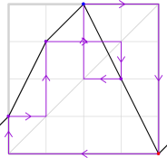
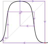
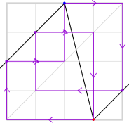
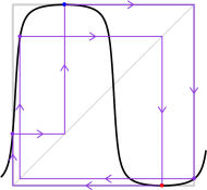
Figure 36: Left: the co-polynomial with combinatorics ${(\!(}1,\,3,\,4,\,2,\,0{)\!)}$, mapping pattern $\underline{\underline{x_{4}}}\mapsto x_{0}\mapsto x_{1}\mapsto x_{3}\mapsto\underline{\underline{x_{2}}}\mapsto\underline{\underline{x_{4}}}$ and topological shape $+-$ . Right: combinatorics ${(\!(}2,\,3,\,4,\,0,\,1{)\!)}$, mapping pattern $\underline{\underline{x_{3}}}\mapsto x_{0}\mapsto\underline{\underline{x_{2}}}\mapsto x_{4}\mapsto x_{1}\mapsto\underline{\underline{x_{3}}}$, and shape $+-+$ .

(Compare Figure 36-left.) In this case, we have $\nu(x_{0})=2$ but $\nu(x_{1})=\nu(x_{2})=\infty$, and it follows that $\chi=-1/2<0$.

Douady-Hubbard ([DH, Theorem 1]) asserts that:

If the orbifold is non-Euclidean, then either:

• the iterated pull-back transformation converges, yielding a rational map with the specified combinatorics; or

• there is no such rational map.

However they make no such assertion in the Euclidean case where $\chi=0$. We will prove the following for real quadratic combinatorics.

Lemma .

The only admissible, minimal and non-polynomial combinatorics with $\chi=0$ are ${(\!(}1,\,0{)\!)}$, ${(\!(}2,\,3,\,2,\,0{)\!)}$, and ${(\!(}1,\,3,\,4,\,3,\,1,\,0{)\!)}$; together with the corresponding cases with reversed orientation.

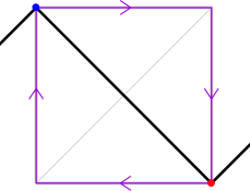
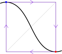
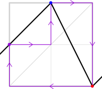
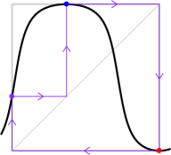
Figure 33: Co-polynomial maps. On the left are illustrations of a piece-wise linear map and its corresponding rational map for the combinatorics ${(\!(}1,\,0{)\!)}$ of topological shape $-$ and mapping pattern $\underline{\underline{x_{0}}}\leftrightarrow\underline{\underline{x_{1}}}$ . On the right are illustrations of a map of topological shape $+-$  for combinatorics ${(\!(}1,\,2,\,0{)\!)}$ with mapping pattern $\underline{\underline{x_{2}}}\mapsto x_{0}\mapsto\underline{\underline{x_{1}}}\mapsto\underline{\underline{x_{2}}}$ .

(Compare Figures 33-left, 42-left, and 12.)

Proof.

Since our maps are quadratic, the ramification index of a postcritical point can only take the values 2, 4, or $\infty$. It will be convenient to set

• equal to the number of “simply postcritical” points with $\nu=2$,

• the number of “doubly postcritical” points with $\nu=4$, and

• the number of “infinitely postcritical” points with $\nu=\infty$.

Then the formula (5.3) becomes

$$\chi~{}=~{}2-\frac{1}{2}~{}\textbf{s}-\frac{3}{4}~{}\textbf{d}-\textbf{i}~{}.$$

First consider combinatorics of Type B or D. Then all $n+1$ of the marked points are infinitely postcritical, so that $\chi=1-n$. Thus $\chi=0$ only for $n=1$, with combinatorics ${(\!(}1,\,0{)\!)}$.

Next consider Type C.   Since critical fixed points have been excluded, there must be a periodic critical orbit with period at least two; thus $~{}{\bf i}\geq 2$. Furthermore, the other critical point can’t map directly to this periodic orbit, so that $~{}{\bf s}\geq 1$; and it follows that $\chi\leq-1/2$.

Similarly in the Half-Hyperbolic case we have $~{}~{}{\bf i}\geq 2$ and $~{}{\bf s}\geq 2$, so $\chi\leq-1$.

There remains the Totally Non-Hyperbolic case. Since neither critical point can map directly to a periodic cycle, and since at most one point can map to a fixed point, the only possible mapping patterns with $\chi=0$ are the following:

(5.4)

or

  (5.5)

or

$$\lx@xy@svg{\hbox{\raise 0.0pt\hbox{\kern 5.5pt\hbox{\ignorespaces\ignorespaces\ignorespaces\hbox{\vtop{\kern 0.0pt\offinterlineskip\halign{\entry@#!@&&\entry@@#!@\cr&&&&&\crcr}}}\ignorespaces{\hbox{\kern-5.5pt\raise 0.0pt\hbox{\hbox{\kern 0.0pt\raise 0.0pt\hbox{\hbox{\kern 3.0pt\raise 0.0pt\hbox{$\textstyle{\underline{\underline{c_{1}}}\ignorespaces\ignorespaces\ignorespaces\ignorespaces}$}}}}}}}\ignorespaces\ignorespaces\ignorespaces\ignorespaces{\hbox{\kern 5.50002pt\raise 0.0pt\hbox{\hbox{\kern 0.0pt\raise 0.0pt\hbox{\lx@xy@stopper}}}}}{\hbox{\lx@xy@droprule}}\ignorespaces{\hbox{\kern 29.5pt\raise 0.0pt\hbox{\hbox{\kern 0.0pt\raise 0.0pt\hbox{\lx@xy@tip{1}\lx@xy@tip{-1}}}}}}{\hbox{\lx@xy@droprule}}{\hbox{\lx@xy@droprule}}{\hbox{\kern 29.5pt\raise 0.0pt\hbox{\hbox{\kern 0.0pt\raise 0.0pt\hbox{\hbox{\kern 3.0pt\raise 0.0pt\hbox{$\textstyle{v_{1}\ignorespaces\ignorespaces\ignorespaces\ignorespaces}$}}}}}}}\ignorespaces\ignorespaces\ignorespaces\ignorespaces{\hbox{\kern 43.50601pt\raise 0.0pt\hbox{\hbox{\kern 0.0pt\raise 0.0pt\hbox{\lx@xy@stopper}}}}}{\hbox{\lx@xy@droprule}}\ignorespaces{\hbox{\kern 67.50601pt\raise 0.0pt\hbox{\hbox{\kern 0.0pt\raise 0.0pt\hbox{\lx@xy@tip{1}\lx@xy@tip{-1}}}}}}{\hbox{\lx@xy@droprule}}{\hbox{\lx@xy@droprule}}{\hbox{\kern 67.50601pt\raise 0.0pt\hbox{\hbox{\kern 0.0pt\raise 0.0pt\hbox{\hbox{\kern 3.0pt\raise 0.0pt\hbox{$\textstyle{x\ignorespaces\ignorespaces\ignorespaces\ignorespaces}$}}}}}}}\ignorespaces\ignorespaces\ignorespaces\ignorespaces{\hbox{\kern 79.22128pt\raise 0.0pt\hbox{\hbox{\kern 0.0pt\raise 0.0pt\hbox{\lx@xy@tip{1}\lx@xy@tip{-1}}}}}}{\hbox{\lx@xy@droprule}}\ignorespaces{\hbox{\kern 103.22128pt\raise 0.0pt\hbox{\hbox{\kern 0.0pt\raise 0.0pt\hbox{\lx@xy@tip{1}\lx@xy@tip{-1}}}}}}{\hbox{\lx@xy@droprule}}{\hbox{\lx@xy@droprule}}{\hbox{\kern 103.22128pt\raise 0.0pt\hbox{\hbox{\kern 0.0pt\raise 0.0pt\hbox{\hbox{\kern 3.0pt\raise 0.0pt\hbox{$\textstyle{y}$}}}}}}}{\hbox{\kern 138.48288pt\raise 0.0pt\hbox{\hbox{\kern 0.0pt\raise 0.0pt\hbox{\hbox{\kern 3.0pt\raise 0.0pt\hbox{$\textstyle{v_{2}\ignorespaces\ignorespaces\ignorespaces\ignorespaces}$}}}}}}}\ignorespaces\ignorespaces\ignorespaces\ignorespaces{\hbox{\kern 138.48288pt\raise 0.0pt\hbox{\hbox{\kern 0.0pt\raise 0.0pt\hbox{\lx@xy@stopper}}}}}{\hbox{\lx@xy@droprule}}\ignorespaces{\hbox{\kern 114.48288pt\raise 0.0pt\hbox{\hbox{\kern 0.0pt\raise 0.0pt\hbox{\lx@xy@tip{1}\lx@xy@tip{-1}}}}}}{\hbox{\lx@xy@droprule}}{\hbox{\lx@xy@droprule}}{\hbox{\kern 176.48889pt\raise 0.0pt\hbox{\hbox{\kern 0.0pt\raise 0.0pt\hbox{\hbox{\kern 3.0pt\raise 0.0pt\hbox{$\textstyle{\underline{\underline{c_{2}}}\ignorespaces\ignorespaces\ignorespaces\ignorespaces}$}}}}}}}\ignorespaces\ignorespaces\ignorespaces\ignorespaces{\hbox{\kern 176.48889pt\raise 0.0pt\hbox{\hbox{\kern 0.0pt\raise 0.0pt\hbox{\lx@xy@stopper}}}}}{\hbox{\lx@xy@droprule}}\ignorespaces{\hbox{\kern 152.48889pt\raise 0.0pt\hbox{\hbox{\kern 0.0pt\raise 0.0pt\hbox{\lx@xy@tip{1}\lx@xy@tip{-1}}}}}}{\hbox{\lx@xy@droprule}}{\hbox{\lx@xy@droprule}}\ignorespaces}}}}\ignorespaces~{}. \textstyle{\underline{\underline{c_{1}}}\ignorespaces\ignorespaces\ignorespaces\ignorespaces} \textstyle{v_{1}\ignorespaces\ignorespaces\ignorespaces\ignorespaces} \textstyle{x\ignorespaces\ignorespaces\ignorespaces\ignorespaces} \textstyle{y} \textstyle{v_{2}\ignorespaces\ignorespaces\ignorespaces\ignorespaces} \textstyle{\underline{\underline{c_{2}}}\ignorespaces\ignorespaces\ignorespaces\ignorespaces} \textstyle{\underline{\underline{c_{1}}}\ignorespaces\ignorespaces\ignorespaces\ignorespaces} \textstyle{v_{1}\ignorespaces\ignorespaces\ignorespaces\ignorespaces} \textstyle{x\ignorespaces\ignorespaces\ignorespaces\ignorespaces} \textstyle{y} \textstyle{v_{2}\ignorespaces\ignorespaces\ignorespaces\ignorespaces} \textstyle{\underline{\underline{c_{2}}}\ignorespaces\ignorespaces\ignorespaces\ignorespaces}$$ (5.6)

∎

      

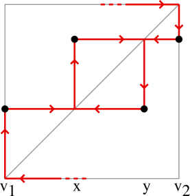
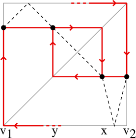
Figure 14: The topologically possible arrangements for a map with mapping pattern (5.6).

Lemma .

There is only one admissible and minimal combinatorics compatible with the mapping pattern (5.4) or with (5.5); but there is none compatible with (5.6).

Proof.

First consider the mapping pattern (5.6). Clearly both $x$ and $y$ must belong to the interval $f({\widehat{\mathbb{R}}})=[v_{1},~{}v_{2}]$ and cannot be equal to $v_{1}$ or $v_{2}$. Furthermore, either $x<y$ as in Figure 14-left, or $x>y$ as in Figure 14-right. The left hand picture is impossible since any compatible graph would have to pass through the four points marked by black dots. But then a horizontal line between levels $x$ and $y$ would have to intersect this graph at least three times: once between the first two points, once between the two middle points, and once between the last two points. This is impossible for any graph which is supposed to imitate a function of degree two.

The right hand figure is possible; but only if the graph is topologically as described by the dotted lines. But then the corresponding combinatorics is not minimal, since the interval $[y,~{}x]$ maps to itself and contains no critical point. Thus there is no minimal solution in this case. (See Figure 6 for further discussion of this combinatorics.)

The proof for (5.5) is similar. If $x<y$, then we see easily that the topological arrangement shown in Figure 12 is the only one possible; while if $x>y$ then we get the $180^{\circ}$ rotation of that figure. This case has been thoroughly discussed in Section 5.

Finally, for (5.4), if we write the mapping pattern as

$$~{}\lx@xy@svg{\hbox{\raise 0.0pt\hbox{\kern 5.5pt\hbox{\ignorespaces\ignorespaces\ignorespaces\hbox{\vtop{\kern 0.0pt\offinterlineskip\halign{\entry@#!@&&\entry@@#!@\cr&&&\crcr}}}\ignorespaces{\hbox{\kern-5.5pt\raise 0.0pt\hbox{\hbox{\kern 0.0pt\raise 0.0pt\hbox{\hbox{\kern 3.0pt\raise 0.0pt\hbox{$\textstyle{\underline{\underline{c_{2}}}\ignorespaces\ignorespaces\ignorespaces\ignorespaces}$}}}}}}}\ignorespaces\ignorespaces\ignorespaces\ignorespaces{\hbox{\kern 5.50002pt\raise 0.0pt\hbox{\hbox{\kern 0.0pt\raise 0.0pt\hbox{\lx@xy@stopper}}}}}{\hbox{\lx@xy@droprule}}\ignorespaces{\hbox{\kern 29.5pt\raise 0.0pt\hbox{\hbox{\kern 0.0pt\raise 0.0pt\hbox{\lx@xy@tip{1}\lx@xy@tip{-1}}}}}}{\hbox{\lx@xy@droprule}}{\hbox{\lx@xy@droprule}}{\hbox{\kern 29.5pt\raise 0.0pt\hbox{\hbox{\kern 0.0pt\raise 0.0pt\hbox{\hbox{\kern 3.0pt\raise 0.0pt\hbox{$\textstyle{(v_{2}=\underline{\underline{c_{1}}})\ignorespaces\ignorespaces\ignorespaces\ignorespaces}$}}}}}}}\ignorespaces\ignorespaces\ignorespaces\ignorespaces{\hbox{\kern 64.06163pt\raise 0.0pt\hbox{\hbox{\kern 0.0pt\raise 0.0pt\hbox{\lx@xy@stopper}}}}}{\hbox{\lx@xy@droprule}}\ignorespaces{\hbox{\kern 88.06161pt\raise 0.0pt\hbox{\hbox{\kern 0.0pt\raise 0.0pt\hbox{\lx@xy@tip{1}\lx@xy@tip{-1}}}}}}{\hbox{\lx@xy@droprule}}{\hbox{\lx@xy@droprule}}{\hbox{\kern 88.06161pt\raise 0.0pt\hbox{\hbox{\kern 0.0pt\raise 0.0pt\hbox{\hbox{\kern 3.0pt\raise 0.0pt\hbox{$\textstyle{v_{1}\ignorespaces\ignorespaces\ignorespaces\ignorespaces}$}}}}}}}\ignorespaces\ignorespaces\ignorespaces\ignorespaces{\hbox{\kern 102.06763pt\raise 0.0pt\hbox{\hbox{\kern 0.0pt\raise 0.0pt\hbox{\lx@xy@stopper}}}}}{\hbox{\lx@xy@droprule}}\ignorespaces{\hbox{\kern 126.06763pt\raise 0.0pt\hbox{\hbox{\kern 0.0pt\raise 0.0pt\hbox{\lx@xy@tip{1}\lx@xy@tip{-1}}}}}}{\hbox{\lx@xy@droprule}}{\hbox{\lx@xy@droprule}}{\hbox{\kern 126.06763pt\raise 0.0pt\hbox{\hbox{\kern 0.0pt\raise 0.0pt\hbox{\hbox{\kern 3.0pt\raise 0.0pt\hbox{$\textstyle{x\ignorespaces\ignorespaces\ignorespaces\ignorespaces\ignorespaces\ignorespaces}$}}}}}}}\ignorespaces\ignorespaces\ignorespaces\ignorespaces\ignorespaces\ignorespaces\ignorespaces\ignorespaces\ignorespaces{}{}{}{}{{}{{}{{}{{}{{}}{}{{}{{}}{}{{}{{}}{}{{}{{}}{}{{}}{}{{}}}}}}}}}{}\ignorespaces\hbox{\hbox{\kern 0.0pt\raise 0.0pt\hbox{{}{}{{}}{{}{}{}{}}{}}}}\ignorespaces{}\ignorespaces{}{}{}{}{{}{{}}{}{{}}{}{{}}{}{{}}{}{{}{{}}{}{{}{{}{{}{{}}{}{{}}{}{{}}}}}}}{\hbox{\kern 135.21877pt\raise-2.99599pt\hbox{\hbox{\kern 0.0pt\raise 0.0pt\hbox{\lx@xy@tip{1}\lx@xy@tip{-1}}}}}}\ignorespaces\hbox{\hbox{\kern 0.0pt\raise 0.0pt\hbox{{}{}{}{{}}{{}{}{}{}\lx@xy@spline@}{}}}}\ignorespaces{}\ignorespaces\hbox{\hbox{\kern 0.0pt\raise 0.0pt\hbox{{}{}{{}}{{}{}{}{}}{}}}}\ignorespaces{}\ignorespaces}}}}\ignorespaces~{}~{}~{}~{}~{}, \textstyle{\underline{\underline{c_{2}}}\ignorespaces\ignorespaces\ignorespaces\ignorespaces} \textstyle{(v_{2}=\underline{\underline{c_{1}}})\ignorespaces\ignorespaces\ignorespaces\ignorespaces} \textstyle{v_{1}\ignorespaces\ignorespaces\ignorespaces\ignorespaces} \textstyle{x\ignorespaces\ignorespaces\ignorespaces\ignorespaces\ignorespaces\ignorespaces} \textstyle{\underline{\underline{c_{2}}}\ignorespaces\ignorespaces\ignorespaces\ignorespaces} \textstyle{(v_{2}=\underline{\underline{c_{1}}})\ignorespaces\ignorespaces\ignorespaces\ignorespaces} \textstyle{v_{1}\ignorespaces\ignorespaces\ignorespaces\ignorespaces} \textstyle{x\ignorespaces\ignorespaces\ignorespaces\ignorespaces\ignorespaces\ignorespaces}$$

then we are quickly led to the combinatorics shown in Figure 42-left. This completes the proof of Section 5. ∎

Thus we have explicitly described what happens in the three cases with Euclidean orbifold. This also completes the proof of Section 5, since in all other cases the statement follows from Thurston’s arguments, as described in [DH]. ∎

6 The Moduli Spaces ${\mathcal{M}}$ and ${\mathcal{M}}/{\mathcal{I}}$

Let ${\mathcal{M}}$ be the moduli space for real quadratic maps with real critical points up to orientation preserving change of coordinates. This section will show that ${\mathcal{M}}$ is a smooth manifold with the topology of a cylinder or annulus. On the other hand, if we allow orientation reversing changes of coordinate, then we obtain the quotient manifold ${\mathcal{M}}/{\mathcal{I}}$, which is a simply-connected smooth manifold with boundary. Compare Figures 15 and 17.

We will first prove the following.

Theorem .

Every quadratic map with real coefficients and real critical points is conjugate, under an orientation preserving change of coordinates, to one and only one map in the canonical form

$$f(x)=\frac{A\,x^{2}+B}{C\,x^{2}+D}\quad{\it satisfying}\quad A^{2}+C^{2}\,=\,B^{2}+D^{2}\,,\quad{\sf and}\quad AD-BC\,>\,0~{}.$$

Here $A,~{}B,~{}C,~{}D$ are uniquely determined up to multiplication by a common non-zero constant.

Proof.

Every conjugacy class can be put into the form

$$g(x)~{}=~{}\frac{ax^{2}+b}{cx^{2}+d}$$

by placing its two critical points at zero and infinity. We can always assume that $ad-bc>0$, conjugating $g$ if necessary by the orientation preserving transformation $x\mapsto-1/x$ which interchanges the two critical points and changes the sign of $ad-bc$. (It then follows that $g^{\prime}(x)>0\Leftrightarrow x>0$; assuming that the denominator is not zero.)

Now consider a scale change, replacing $g(x)$ by the map $f(x)=g(\lambda x)/\lambda$ with $\lambda>0$. Then

$$f(x)~{}=~{}\frac{Ax^{2}+B}{Cx^{2}+D}\quad{\rm with}\quad A=\lambda^{2}a,~{}~{}B=b,~{}~{}C=\lambda^{3}c,~{}~{}D=\lambda d~{}.$$

We must choose $\lambda$ so that

$$A^{2}+C^{2}=B^{2}+D^{2}\quad{\rm or~{}equivalently}\quad\lambda^{6}c^{2}+\lambda^{4}a^{2}-\lambda^{2}d^{2}-b^{2}~{}=~{}0\,.$$

Dividing the last equation by $\lambda^{3}$, we get

$$\lambda^{3}c^{2}+\lambda\,a^{2}-d^{2}/\lambda-b^{2}/\lambda^{3}~{}=~{}0~{}.$$

The left side of this equation, considered as a function of $\lambda$, is clearly monotone, mapping the half-line $\lambda>0$ diffeomorphically onto the entire real line. Therefore there is one and only one choice of $\lambda$ which satisfies the equation. This proves that every such map is conjugate to one in canonical form. Since each step of the argument is uniquely determined, uniqueness follows easily. This proves Section 6.∎

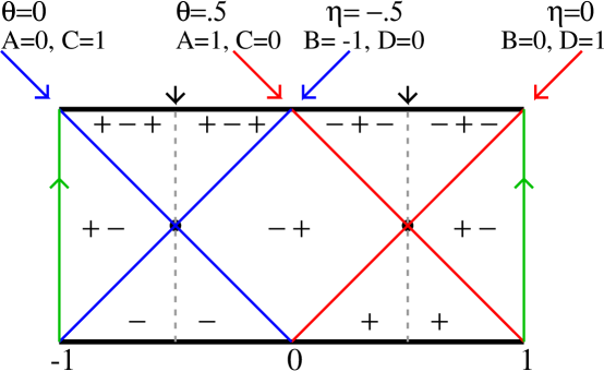
Figure 15: The cylindrical moduli space ${\mathcal{M}}\cong({\mathbb{R}}/2{\mathbb{Z}})\times(0,1)$ can be obtained from the rectangle $[-1,1]\times[0,1]$ in the $(\Sigma,\,\Delta)$-plane by identifying the left and right edges $\Sigma=\pm 1$ so that the arrows match. Here the top and bottom edges represent points in the ideal boundary of ${\mathcal{M}}$. The red lines represent maps of polynomial shape. They cross each other at the point $\langle x\mapsto x^{2}\rangle$. The blue lines represent maps of co-polynomial shape, with one critical point mapping to the other. These lines cross at the point $\langle x\mapsto-1/x^{2}\rangle$. The four red and blue lines divide ${\mathcal{M}}$ into six complementary regions, each either monotone, unimodal, or bimodal of the shape indicated. The dotted lines form the symmetry locus, consisting of conjugacy classes which are invariant under reflection in either of these lines (or under the orientation reversing transformation $(\Sigma,\,\Delta)\leftrightarrow(\pm 1-\Sigma,\,\Delta)$). The small black arrows point to what we believe are the only possible limit points of the iterated pullback in the strongly obstructed case. (See Section 7.)

Using this result, we can provide an explicit description for the moduli space ${\mathcal{M}}$ consisting of all conjugacy classes of real quadratic maps. First note that we can always normalize so that $A^{2}+C^{2}=B^{2}+D^{2}=1$ by multiplying $A,B,C,D$ by a suitable common constant. It is then natural to choose angles $\theta$ and $\eta$ so that

$$A=\sin(\pi\theta),~{}~{}C=\cos(\pi\theta)~{},\qquad{\rm and}\qquad B=\sin(\pi\eta),~{}~{}D=\cos(\pi\eta)~{}.$$

Here it is necessary to be careful. If we add one to both $\theta$ and $\eta$, then the constants $A,~{}B,~{}C,~{}D$ will all be multiplied by $-1$, and the map $f$ will not change. However, if we replace $(\theta,~{}\eta)$ by $(\theta+1,~{}\eta)$, then we will get a quite different map.

Note also that the determinant can be written as

$$AD-BC~{}=~{}\sin(\pi\theta)\cos(\pi\eta)-\cos(\pi\theta)\sin(\pi\eta)~{}=~{}\sin\big{(}\pi(\theta-\eta)\big{)}~{}.$$

Since we require that $AD-BC>0$, it will be convenient to assume that

$$\theta-\eta~{}=~{}\Delta\qquad{\rm with}\qquad 0<\Delta<1~{}.$$

On the other hand, since we can’t add one to $\theta$ without also adding one to $\eta$, it follows that the sum $\Sigma=\theta+\eta$ is actually well defined modulo two. This proves the following

Corollary .

A map in the normal form of Section 6 is uniquely determined by the two invariants

$$\Sigma~{}=~{}\theta+\eta~{}\in~{}{\mathbb{R}}/(2{\mathbb{Z}})\qquad{\rm and}\qquad\Delta~{}=~{}\theta-\eta~{}\in~{}(0,1)~{}.$$

Therefore the moduli space ${\mathcal{M}}$, consisting of all conjugacy classes of quadratic maps with real coefficients and real critical points, is diffeomorphic to the cylinder $({\mathbb{R}}/2{\mathbb{Z}})\times(0,1)~{}$. ˜

We can provide a more geometric interpretation of the invariants $\theta$, $\eta$, $\Sigma$, and $\Delta$ as follows. We make use of three different closely related models for ${\widehat{\mathbb{R}}}$. By definition ${\widehat{\mathbb{R}}}={\mathbb{R}}\cup\{\infty\}$. However, ${\widehat{\mathbb{R}}}$ can be identified with the standard circle ${\mathbb{R}}/{\mathbb{Z}}$ by letting $t\in{\mathbb{R}}/{\mathbb{Z}}$ correspond to $\tan(\pi\,t)\in{\widehat{\mathbb{R}}}$; and can also be identified with the real projective line by letting $t$ correspond to the ratio

$$\big{(}\sin(\pi\,t)~{}:~{}\cos(\pi\,t)\big{)}~{}\in~{}{\mathbb{P}}^{1}({\mathbb{R}})~{}.$$

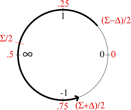
Figure 16: Identifying $\widehat{\mathbb{R}}$ with the unit circle, or with ${\mathbb{R}}/{\mathbb{Z}}$. Several points $x\in\widehat{\mathbb{R}}$ are indicated in black, inside the circle, while the corresponding coordinates $t\in{\mathbb{R}}/{\mathbb{Z}}$, with $\tan(\pi t)=x$, are indicated in red, outside. The basic invariant for a map in canonical form is the image $f({\widehat{\mathbb{R}}})$, indicated here (for a typical example of shape $+-+$) by a heavy black arc. The length of this arc in ${\mathbb{R}}/{\mathbb{Z}}$ coordinates is equal to $\Delta\in(0,1)$, and its midpoint is $\Sigma/2$.

Corollary .

If $f$ is in canonical form, then the image $f({\widehat{\mathbb{R}}})\subset{\widehat{\mathbb{R}}}\cong{\mathbb{P}}^{1}$ is the circle arc of length $\Delta$ in ${\mathbb{R}}/{\mathbb{Z}}$ coordinates, with end points $\eta$ and $\theta$, and with mid point $\Sigma/2$.

Compare Figure 16. Since $\Sigma$ is well defined mod $2{\mathbb{Z}}$, it follows that $\Sigma/2$ is well defined mod ${\mathbb{Z}}$.

Proof of Section 6.

The end points of $f({\widehat{\mathbb{R}}})$ are the critical values

$$f(0)~{}=~{}B/D~{}=~{}\big{(}\sin(\pi\eta):\cos(\pi\eta)\big{)}\quad{\rm and}\quad f(\infty)~{}=~{}A/C~{}=~{}\big{(}\sin(\pi\theta):\cos(\pi\theta)\big{)}~{},$$

corresponding to the points $t=\eta$ and $t=\theta$ in ${\mathbb{R}}/{\mathbb{Z}}$. These two points divide the circle into two arcs. We must check that $\Sigma/2$ is the center point of the arc corresponding to $f({\widehat{\mathbb{R}}})$, which has length $\Delta$. It is enough to check this for a single example, since all other cases will then follow by continuity. As our example, for $f(x)=x^{2}$ with $A=D=1$ and $B=C=0$, it is not hard to check that

$$\eta=0\,,\quad\theta=1/2\,,\quad{\rm and}\quad\Sigma=\Delta=1/2~{}.$$

On the other hand, $f({\widehat{\mathbb{R}}})=[0,\,+\infty]$ corresponds to the interval $0\leq t\leq 1/2$, with center point at $\Sigma/2=1/4$, as required. This completes the proof. ∎

Orientation Reversal: The Canonical Involution ${\mathcal{I}}$.

Let $\langle f\rangle\in{\mathcal{M}}$ denote the conjugacy class of $f$, and let $J:{\widehat{\mathbb{R}}}\to{\widehat{\mathbb{R}}}$ be any orientation reversing fractional linear transformation. There is a canonical involution ${\mathcal{I}}$ of ${\mathcal{M}}$ defined by the equation

$${\mathcal{I}}\big{(}\langle f\rangle\big{)}~{}=~{}\langle J\circ f\circ J\rangle~{}.$$

This conjugacy class does not depend on the choice of $J$. If $J^{\prime}$ is another involution and if $L=J\circ J^{\prime}$ with $L^{-1}=J^{\prime}\circ J$, then evidently

$$L\circ(J^{\prime}\circ f\circ J^{\prime})\circ L^{-1}~{}=~{}J\circ f\circ J~{},$$

so the two are conjugate. For example we could take $J(x)=-x$ or $1/x$. If we consider maps normalized so that $f({\widehat{\mathbb{R}}})=[0,1]$, then the most convenient choice is $J(x)=1-x$, corresponding to a $180^{\circ}$ rotation of the graph of $f$.

The fixed points of ${\mathcal{I}}$ form the symmetry locus. The conjugacy class $\langle f\rangle$ belongs to this symmetry locus if and only if $f$ commutes with some orientation reversing fractional linear transformation, which necessarily interchanges the two critical points of $f$.

Remark .

This orientation reversing involution also reverses combinatorics, replacing ${(\!(}m_{0},\ldots,m_{n}{)\!)}$ by the sequence

$${(\!(}n-m_{n}\,,~{}~{}n-m_{n-1}\,,~{}~{}\ldots\,,~{}~{}n-m_{1}\,,~{}~{}n-m_{0}{)\!)}~{}.$$

It acts on the Epstein parameters by sending $(\mu,\,\kappa)$ to $(\mu,\,-\kappa)$.

Definition .

Let ${\mathcal{M}}/{\mathcal{I}}$ be the quotient in which each conjugacy class $\langle f\rangle$ is identified with ${\mathcal{I}}(\langle f\rangle)$. This is the appropriate moduli space to work with when studying properties which do not depend on orientation. Since the involution ${\mathcal{I}}$ acts on the cylinder by mapping each pair $(\Sigma,\,\Delta)\in({\mathbb{R}}/2{\mathbb{Z}})\times(0,1)$ to the pair $(1-\Sigma,\,\Delta)$. It follows that each pair $(\langle f\rangle,~{}{\mathcal{I}}\langle f\rangle)$ has a unique representative for which $|\Sigma|\leq 0.5$. In other words, the middle half of Figure 15, consisting of pairs $(\Sigma,~{}\Delta)$ with $|\Sigma|\leq 0.5$, maps bijectively onto ${\mathcal{M}}/{\mathcal{I}}$.

\begin{overpic}[width=289.07999pt]{Per1cheb-b-crop.pdf} \put(180.0,265.0){$\rm SL$} \put(100.0,265.0){$\rm SL$} \put(140.0,265.0){$\rm SL$} \put(213.0,220.0){${\mathscr{F}}(1,2)$} \put(245.0,190.0){${\mathscr{F}}(2,1)$} \put(125.0,150.0){\rm unimodal} \put(80.0,190.0){${\mathscr{F}}(0,1)$} \put(125.0,90.0){${\mathscr{F}}(1,0)$} \put(128.0,50.0){$J_{\mathbb{R}}=\emptyset$} \end{overpic}

Figure 17: The quotient space ${\mathcal{M}}/{\mathcal{I}}$ can be identified with the square region $[-.5,~{}.5]\times(0,1)$ between the two dotted green lines of Figure 15. In the figure above, the black curve ${\bf Per}_{1}(1)$ and the green curve ${\bf Per}_{1}(-1)$ divide ${\mathcal{M}}/{\mathcal{I}}$ into four regions ${\mathscr{F}}({\bf a},\,{\bf r})$, distinguished by the number of attracting and repelling fixed points; while the dotted red and blue lines divide it independently into five regions, with the unimodal region in the center. The left and right boundaries form the symmetry locus and are part of ${\mathcal{M}}/{\mathcal{I}}$; but the top and bottom boundaries represent ideal limit points. The shift locus $\rm SL$ is the subset of ${\mathscr{F}}(1,2)$ which lies above both ${\bf Per}_{1}(1)$ and the gray Chebyshev curve. It intersects the $+-+$, unimodal, and $-+-$ regions. (See Section 6.)

Remark (Important subsets of ${\mathcal{M}}/{\mathcal{I}}$).

For a picture of ${\mathcal{M}}/{\mathcal{I}}$ see Figure 17. (Compare the older picture of ${\mathcal{M}}/{\mathcal{I}}$ in Figure 20; but be warned that comparison of the two pictures can be very confusing.) Just as in Figure 15, the diagonal lines representing conjugacy classes of polynomial and co-polynomial shape divide the figure into bimodal, unimodal and monotone regions. However in this case there are only five such regions since we no longer distinguish between $+-$ unimodal and $-+$ unimodal.

There is a quite different subdivision of ${\mathcal{M}}/{\mathcal{I}}$ as follows. The black curve in Figure 17 represents ${\bf Per}_{1}(+1)$, the set of all conjugacy classes with a fixed point of multiplier $+1$; and similarly the green curve represents ${\bf Per}_{1}(-1)$. These curves divide ${\mathcal{M}}/{\mathcal{I}}$ into four “fixed point regions”, which we denote by ${\mathscr{F}}({\bf a},~{}{\bf r})$, where ${\bf a}$ is the number of attracting fixed points of $f$ for $\langle f\rangle$ in this region, and ${\bf r}$ is the number of repelling fixed points. Here the lower region ${\mathscr{F}}(1,0)$ is dynamically rather boring. It consists of maps for which the topological entropy is zero and the real Julia set $J_{\mathbb{R}}$ is empty. (All real orbits converge to the unique attracting fixed point.) The right hand region ${\mathscr{F}}(2,1)$ is somewhat more interesting. Here $J_{\mathbb{R}}$ consists of one repelling fixed point in $f({\widehat{\mathbb{R}}})$ and its one preimage. The orbit of every point in ${\widehat{\mathbb{R}}}{\smallsetminus}J_{\mathbb{R}}$ converges to one of the two attracting fixed points.

The two regions ${\mathscr{F}}(0,1)$ and ${\mathscr{F}}(1,2)$ above the green curve are much more interesting. In particular, every critically finite class which is not of polynomial shape must be contained in ${\mathscr{F}}(0,1)$; while every one which is of polynomial shape must be contained in ${\mathscr{F}}(1,2)$ (except in the special case of $\langle x\mapsto x^{2}\rangle$).

There is an important sub-region of ${\mathscr{F}}(1,2)$. The hyperbolic shift locus, labeled as ${\rm SL}$, is the open subset consisting all conjugacy classes ${\langle}f{\rangle}$ for which:

• all orbits in ${\widehat{\mathbb{R}}}{\smallsetminus}J_{\mathbb{R}}$ converge to the unique attracting fixed point; and

• if we put the critical points at zero and infinity, then every orbit $x_{0}\mapsto x_{1}\mapsto\cdots$ in $J_{\mathbb{R}}$ is uniquely determined by the sequence of signs $({\rm sgn}(x_{0}),\,{\rm sgn}(x_{1}),\,\cdots)$, where any such sequence can occur.

The closure $\overline{SL}$ is the set of pf points with maximal topological entropy $\log(2)$. (See [F, Prop. 3.6].) The boundary of the hyperbolic shift locus within ${\mathcal{M}}/{\mathcal{I}}$ is a piecewise analytic curve. The left part of the boundary is a subset of ${\bf Per}_{1}(1)$ called the parabolic shift locus. The right part of the boundary (the gray curve in our figure) will be called the Chebyshev curve. It consists of all $\langle f\rangle$ which have one critical orbit of the form

$$~{}\lx@xy@svg{\hbox{\raise 0.0pt\hbox{\kern 5.5pt\hbox{\ignorespaces\ignorespaces\ignorespaces\hbox{\vtop{\kern 0.0pt\offinterlineskip\halign{\entry@#!@&&\entry@@#!@\cr&&\crcr}}}\ignorespaces{\hbox{\kern-5.5pt\raise 0.0pt\hbox{\hbox{\kern 0.0pt\raise 0.0pt\hbox{\hbox{\kern 3.0pt\raise 0.0pt\hbox{$\textstyle{\underline{\underline{c_{1}}}\ignorespaces\ignorespaces\ignorespaces\ignorespaces}$}}}}}}}\ignorespaces\ignorespaces\ignorespaces\ignorespaces{\hbox{\kern 5.50002pt\raise 0.0pt\hbox{\hbox{\kern 0.0pt\raise 0.0pt\hbox{\lx@xy@stopper}}}}}{\hbox{\lx@xy@droprule}}\ignorespaces{\hbox{\kern 29.5pt\raise 0.0pt\hbox{\hbox{\kern 0.0pt\raise 0.0pt\hbox{\lx@xy@tip{1}\lx@xy@tip{-1}}}}}}{\hbox{\lx@xy@droprule}}{\hbox{\lx@xy@droprule}}{\hbox{\kern 29.5pt\raise 0.0pt\hbox{\hbox{\kern 0.0pt\raise 0.0pt\hbox{\hbox{\kern 3.0pt\raise 0.0pt\hbox{$\textstyle{v_{1}\ignorespaces\ignorespaces\ignorespaces\ignorespaces}$}}}}}}}\ignorespaces\ignorespaces\ignorespaces\ignorespaces{\hbox{\kern 43.50601pt\raise 0.0pt\hbox{\hbox{\kern 0.0pt\raise 0.0pt\hbox{\lx@xy@stopper}}}}}{\hbox{\lx@xy@droprule}}\ignorespaces{\hbox{\kern 67.50601pt\raise 0.0pt\hbox{\hbox{\kern 0.0pt\raise 0.0pt\hbox{\lx@xy@tip{1}\lx@xy@tip{-1}}}}}}{\hbox{\lx@xy@droprule}}{\hbox{\lx@xy@droprule}}{\hbox{\kern 67.50601pt\raise 0.0pt\hbox{\hbox{\kern 0.0pt\raise 0.0pt\hbox{\hbox{\kern 3.0pt\raise 0.0pt\hbox{$\textstyle{x\ignorespaces\ignorespaces\ignorespaces\ignorespaces\ignorespaces\ignorespaces}$}}}}}}}\ignorespaces\ignorespaces\ignorespaces\ignorespaces\ignorespaces\ignorespaces\ignorespaces\ignorespaces\ignorespaces{}{}{}{}{{}{{}{{}{{}{{}}{}{{}{{}}{}{{}{{}}{}{{}{{}}{}{{}}{}{{}}}}}}}}}{}\ignorespaces\hbox{\hbox{\kern 0.0pt\raise 0.0pt\hbox{{}{}{{}}{{}{}{}{}}{}}}}\ignorespaces{}\ignorespaces{}{}{}{}{{}{{}}{}{{}}{}{{}}{}{{}}{}{{}{{}}{}{{}{{}{{}{{}}{}{{}}{}{{}}}}}}}{\hbox{\kern 76.65715pt\raise-2.99599pt\hbox{\hbox{\kern 0.0pt\raise 0.0pt\hbox{\lx@xy@tip{1}\lx@xy@tip{-1}}}}}}\ignorespaces\hbox{\hbox{\kern 0.0pt\raise 0.0pt\hbox{{}{}{}{{}}{{}{}{}{}\lx@xy@spline@}{}}}}\ignorespaces{}\ignorespaces\hbox{\hbox{\kern 0.0pt\raise 0.0pt\hbox{{}{}{{}}{{}{}{}{}}{}}}}\ignorespaces{}\ignorespaces}}}}\ignorespaces~{}~{}~{}~{}~{}, \textstyle{\underline{\underline{c_{1}}}\ignorespaces\ignorespaces\ignorespaces\ignorespaces} \textstyle{v_{1}\ignorespaces\ignorespaces\ignorespaces\ignorespaces} \textstyle{x\ignorespaces\ignorespaces\ignorespaces\ignorespaces\ignorespaces\ignorespaces} \textstyle{\underline{\underline{c_{1}}}\ignorespaces\ignorespaces\ignorespaces\ignorespaces} \textstyle{v_{1}\ignorespaces\ignorespaces\ignorespaces\ignorespaces} \textstyle{x\ignorespaces\ignorespaces\ignorespaces\ignorespaces\ignorespaces\ignorespaces}$$

where $x$ is a fixed point with multiplier $\mu>1$. (This curve intersects the locus of polynomial shape maps precisely in the class of the Chebyshev map $x\mapsto x^{2}-2$.)

Remark (Computing with Epstein coordinates).

For computational purposes, Epstein coordinates, with

$$f(x)=\mu x/(1+2\kappa x+x^{2})~{},$$

are often convenient. One useful quantity is the discriminant

$$D~{}=~{}\mu+\kappa^{2}-1$$

which is positive if there are three real fixed points, negative if there is only one, and zero along the curve ${\bf Per}_{1}(1)$. (Caution: $D$ can be very large for points which are very close to ${\bf Per}_{1}(1)$.) The hyperbolic shift locus is the region defined by the inequalities $\mu>1$ and $|\kappa|>1$. The parabolic shift locus is the part of the boundary of this region with $\mu=1$ and $|\kappa|>1$, while the Chebyshev curve is the rest of the boundary with $|\kappa|=1$ and $\mu\geq 1$. (It extends analytically into the shift locus, but with $\mu<1$).

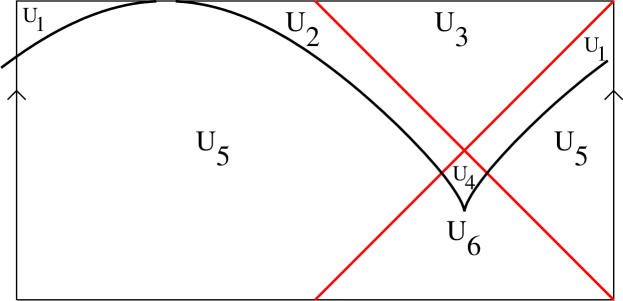
Figure 18: This figure shows a partition of the moduli space ${\mathcal{M}}$ into six regions with the following property: If $\Psi$ is the natural transformation from Epstein coordinates to canonical coordinates, then each branch of $\Psi^{-1}$ is smooth and real analytic within each region.

Remark (Epstein Coordinates $\leftrightarrow$ Canonical Coordinates).

The natural transformation

$$\Psi:(\mu,\,\kappa)~{}\mapsto~{}(\Sigma,\,\Delta)$$

from Epstein coordinates to canonical coordinates is smooth, real analytic, and not too hard to compute. (Compare the proof of Section 6.) But this does not mean that it is easy to understand. Given a real quadratic map $f$ and a non-critical fixed point $x_{0}=f(x_{0})$, we can choose coordinates which place the critical points at $\pm 1$ and place $x_{0}$ at the origin, and then compute the corresponding Epstein coordinates. If ${\langle}f{\rangle}$ lies below the curve ${\bf Per}_{1}(1)$ in moduli space, then there is only one real fixed point, so that $\Psi^{-1}{\langle}f{\rangle}$ is uniquely defined. But if ${\langle}f{\rangle}$ is above ${\bf Per}_{1}(1)$ then there are three distinct real fixed points, so that generically there are three different branches of $\Psi^{-1}$. Points on the polynomial locus provide an additional complication, since one of their fixed points is critical, and hence doesn’t correspond to any choice of Epstein coordinates.

However, if we remove both the (red) polynomial locus and the (black) curve ${\bf Per}_{1}(1)$ from ${\mathcal{M}}$, as illustrated in Figure 18, then we are left with the complementary open set which has six connected components $U_{j}$. In some sense, the inverse map is well behaved and real analytic on each of these components. More precisely, $\Psi^{-1}$ is uniquely defined on the lower regions $U_{5}$ and $U_{6}$, and has three distinct well defined branches on each of the upper regions $U_{1}$, $U_{2}$, $U_{3}$, $U_{4}$. Here the image $\Psi^{-1}(U_{5})$ is contained in the left half-plane $\mu<0$; while $\Psi^{-1}(U_{6})$ is contained in the right half-plane $\mu>0$. For $U_{3}$ (which is precisely the $-+-$ region), two of the branches of $\Psi^{-1}$ map to the left half-plane, and one maps to the right half-plane. Similarly, for $U_{1}$ and $U_{2}$, which intersect the $+-+$ region, two branches map to the right and one to the left. On the other hand, for $U_{4}$ which lies in the $+$ monotone region, all three branches map to the right half-plane.

We will be particularly interested in asymptotic behavior as $\mu\to\pm\infty$.

Theorem .

As $\mu\to\pm\infty$ with $\kappa$ fixed:

• the pair $(\Sigma,~{}\Delta)$ converges to $(\pm.5,~{}1)$,

• the difference ratio $\displaystyle{\frac{\pm.5-\Sigma}{1-\Delta}}$ converges to $-\kappa$, and

• the product $|\mu|(1-\Delta)$ converges to $4/\pi$.

Proof.

Start with $~{}f(x)=\mu\,x/(1+2\,\kappa\,x+x^{2})~{}$. Let $~{}p=2(1+\kappa)~{}$ and $~{}q=2(1-\kappa)$, so that $p+q=4$ and $p-q=4\,\kappa$. The orientation preserving automorphism

$$L(x)~{}=~{}(1+x)/(1-x)\quad{\rm satisfies}\quad L~{}:~{}0\mapsto 1\mapsto\infty\mapsto-1\mapsto 0~{}.$$

Furthermore

$$L\circ f\circ L^{-1}(x)~{}=~{}\frac{a\,x^{2}+b}{c\,x^{2}+d}~{},\qquad{\rm with}\qquad\begin{matrix}a=p+\mu,&b=q-\mu,\\ c=p-\mu,&d=q+\mu.\end{matrix}$$ (6.1)

Following the proof of Section 6, we must now solve the equation

$$u^{3}\,c^{2}~{}+~{}u\,a^{2}~{}-~{}d^{2}/u~{}-~{}b^{2}/u^{3}~{}=~{}0~{}.$$ (6.2)

It will be convenient to make the substitutions $\mu=1/s$ and $u=e^{t}$. Multiplying equation (6.2) by $s^{2}=1/\mu^{2}$, it takes the form

$$e^{3\,t}(1-s\,p)^{2}+e^{t}(1+s\,p)^{2}-e^{-t}(1+s\,q)^{2}-e^{-3\,t}(1-s\,q)^{2}~{}=~{}0~{}.$$

For each fixed value of $\kappa$, the left side of this equation is clearly a real analytic function $\Omega(s,t)$ which can be expanded in an everywhere convergent power series

$$\Omega(s,t)~{}=~{}\sum_{i,j=0}^{\infty}\omega_{i,j}s^{i}t^{j}~{}.$$

It is not difficult to compute the first few coefficients:

$\omega_{0,0}=0$	$\omega_{0,1}=8$	$\omega_{0,2}=0$
$\omega_{1,0}=0$	$\omega_{1,1}=-16$
$\omega_{2,0}=32\,\kappa$

,

so that

$$\Omega(s,t)/8=t\,(1-2\,\,s)+4\,\kappa\,s^{2}+({\rm higher~{}order~{}terms})~{}=~{}0~{}.$$

This implies the asymptotic equality

$$t~{}\simeq~{}-4\kappa\,s^{2}/(1-2s)~{}\simeq~{}-4\,\kappa\,s^{2}\quad{\rm as}\quad t,~{}s~{}\to 0~{}.$$

Thus, if we ignore terms of order $s^{2}$ then we can just take $t=0$ hence $u=1$. This means that we can just use the original values of $a,~{}b,~{}c,~{}d$ as given in Equation (missing) 6.1. The angle $\theta$ can now be computed, modulo $1/2$, by the equation

$$\tan(\pi\,\theta)~{}=~{}a/c~{}=~{}(p+\mu)/(p-\mu)~{}=~{}(p\,s+1)/(p\,s-1)~{}=~{}-1-2\,p\,s+O(s^{2})~{},$$

or equivalently

$$\theta~{}\equiv~{}\frac{1}{\pi}\arctan(-1-2\,p\,s)+O(s^{2})\quad({\rm mod}~{}\scriptsize{\frac{1}{2}}\,{\mathbb{Z}})~{}.$$

Note. For a direct computation of $\theta\in{\mathbb{R}}/{\mathbb{Z}}$ we would have to work with both the sine and cosine functions; but the computation mod 1/2 using the tangent is easier, and will be enough for the proof.

Since $\arctan(-1)=-\pi/4$ and the derivative of $\arctan(x)$ evaluated at $x=-1$ is $1/\big{(}1+(-1)^{2}\big{)}=1/2$, this yields

$$\theta~{}\equiv~{}-.25~{}-~{}p\,s/\pi+O(s^{2})\quad({\rm mod}~{}1/2)~{}~{}.$$

Similarly, since $\tan(\pi\eta)\equiv~{}b/d~{}\equiv~{}(q-\mu)/(q+\mu)$, we get

$$\eta~{}\equiv~{}-.25~{}+~{}q\,s/\pi+O(s^{2}).$$

Therefore

$$\Sigma~{}=~{}\theta+\eta~{}\equiv~{}(q-p)s/\pi\equiv+4\,\kappa\,s/\pi+O(s^{2})\qquad({\rm mod}~{}1/2)~{}~{}.$$

Similarly

$$\Delta~{}=~{}\theta-\eta~{}\equiv~{}-4\,s/\pi+O(s^{2})\qquad({\rm mod}~{}1/2)~{}~{}.$$

What we want is the value of $\Sigma\in{\mathbb{R}}/2{\mathbb{Z}}$ modulo two, and the actual value of $\Delta\in(0,1)$; but each of these formulas may be wrong by an integer or half-integer additive constant. However this constant cannot change as as we vary $s>0$ or as we vary $s<0$. This means that to get the required formulas, we need only choose the right additive constants for any one case with $\mu\to+\infty$ and any one case with $\mu\to-\infty$. The general cases will then follow by continuity. The correct formulas, obtained in this way, are

$$\Sigma~{}=~{}\pm.5+4\,\kappa\,s/\pi+O(s^{2})$$

and

$$\Delta=1-4\,s/\pi+O(s^{2})~{}.$$

Replacing $s$ with $1/\mu$, the theorem as stated follows easily. ∎

Remark (The Filom-Pilgrim Maps).

These form a rich family of critically finite maps of Type B. Given relatively prime numbers $0<p<q$, consider the combinatorics

$${(\!(}p,\,p+1,\,p+2,\,\ldots,\,q-1,\,0,\,1,\,\ldots,\,p-1{)\!)}~{},$$

corresponding to a cyclic permutation of the integers between zero and $q-1$. Filom and Pilgrim [FP] show that this combinatorics is unobstructed in all cases, yielding maps of Type B which they denote by $f_{p/q}$. Note that $f_{p/q}$ is of shape $+-+$ except in the two extreme cases $p=1$ and $p=q-1$ where it is co-polynomial. Under orientation reversal, we have ${\mathcal{I}}{\langle}f_{p/q}{\rangle}={\langle}f_{(q-p)/q}{\rangle}$.

\begin{overpic}[width=397.48499pt]{pmp-topA-crop.pdf} \put(350.0,100.0){\rm SL} \put(45.0,100.0){\rm SL} \end{overpic}

Figure 19: Part of the $+-+$ region in ${\mathcal{M}}$, with $\Delta\geq.75$. The red dots represent those Filom-Pilgrim conjugacy classes ${\rm FP}(p,\,p^{\prime})$ for which the minimum of $p$ and $p^{\prime}$ is $1$; the orange dots represent points with ${\rm min}(p,\,p^{\prime})=2$, and the green points have minimum $3$. On the other hand, the blue dots represent points with $p^{\prime}=p\pm 1$ and with $p,\,p^{\prime}\geq 4$. The black curve is ${\bf Per}_{1}(1)$.

For our purposes it will be convenient to introduce the notation ${\rm FP}(p,\,q-p)$ for the conjugacy class ${\langle}f_{p/q}{\rangle}$ in moduli space. Thus the point ${\rm FP}(p,\,p^{\prime})\in{\mathcal{M}}$ is well defined for every pair of strictly positive coprime integers $p$ and $p^{\prime}$. Here $p^{\prime}$ is the number of iterations needed to map the first critical point to the second, and $p$ is the number needed to map the second critical point back to the first. The orientation reversing involution satisfies ${\mathcal{I}}:{\rm FP}(p,p^{\prime})\leftrightarrow{\rm FP}(p^{\prime},\,p)$

Conjecture .

As $p^{\prime}\to\infty$ with fixed $p$, the conjugacy classes ${\rm FP}(p,p^{\prime})$ tend to a well defined limit ${\rm FP}(p,\,\infty)$ which belongs to the curve ${\bf Per}_{1}(1)$ in moduli space; and similarly, as $p$ tends to infinity with fixed $p^{\prime}$ there is a well defined limit ${\rm FP}(\infty,\,p^{\prime})\in{\bf Per}_{1}(1)$. On the other hand, if both $p$ and $p^{\prime}$ tend to infinity, then the limit is the ideal point with coordinates $(\Sigma,\,\Delta)=(-.5,\,1)$.

We don’t know why these statements should be true; but empirical evidence certainly suggests them. (See Figure 19.) Furthermore the following is known:

Proposition (Filom and Pilgrim).

The topological entropy of $F(p,p^{\prime})$ depends only on the sum $p+p^{\prime}$, and is an explicitly computable number which converges monotonically to $\log(2)$ as $p+p^{\prime}\to\infty$.

See [FP, Proposition 3.2 and Lemma 4.1]. This clearly implies at least that $F(p,p^{\prime})$ converges towards the set ${\bf Per}_{1}(1)$ as $p+p^{\prime}\to\infty$, since the topological entropy is a continuous function on ${\mathcal{M}}$ which takes the value $\log(2)$ only on the closure of the shift locus. (See [F, Prop. 3.6].) For graphs of individual maps see Figures 33R, 34L, 35R, 36R, 37 as well as 25.

Remark .

Here are descriptions of some special points of ${\mathcal{M}}/{\mathcal{I}}$.

• The lower end points of the two curves ${\bf Per}_{1}(\pm 1)$ occur at the conjugacy classes of $\displaystyle{f(x)=\frac{\pm x}{x^{2}+1}}$, with coordinates $(\Sigma,\,\Delta)=(\pm 0.5,\,0.295167)$.

• The center point of the figure, with $(\Sigma,\,\Delta)=(0,\,0.5)$, is represented by the critically finite map $\displaystyle{x\mapsto\frac{x^{2}-1}{x^{2}+1}}$ of Type C. (Compare Figure 38(left).)

• The crossing point between the two curves ${\bf Per}_{1}(\pm 1)$ is represented by the maps $\displaystyle{f(x)=\frac{x}{x^{2}\pm x\sqrt{2}+1}}$, with fixed points of multiplier $1$ at the origin and multiplier $-1$ at $x=\pm\sqrt{2}$. Here $\Sigma$ is 0.25 or 0.75, and $\Delta=0.60817$.

• The crossing point between ${\bf Per}_{1}(1)$ and the locus of co-polynomial points is represented by the map $\displaystyle{x\mapsto\frac{x}{1-3x+x^{2}}}$, with a fixed point of multiplier $1$ at $x=0$. Here $(\Sigma,\,\Delta)=(-0.11353,\,0.88647)$.

• The end point of the Chebyshev curve on ${\bf Per}_{1}(1)$ has coordinates $(0.051576,~{}0.776737)$. This is the only conjugacy class for which the unique fixed point has multiplier one.

Figure 20: A composite moduli space including also maps of degree $\pm 2$. Here the coordinates are the first two symmetric functions of the fixed point multipliers. The vertical line through the class of $z\mapsto z^{2}$ is the locus of polynomial shape maps, while the line through $z\mapsto 1/z^{2}$ is the locus of co-polynomials. The dotted lines of slope $\pm 1$ represent maps with a fixed point of multiplier $\pm 1$. The figure should be cut open along each component of the symmetry locus $\mathcal{S}$: There is a well defined limit as we approach $\mathcal{S}$ from either side; but the two limits are related only by a complex change of coordinate.

Remark (Comparing the two pictures of ${\mathcal{M}}/{\mathcal{I}}$).

Figure 17 can be compared with Figure 20 (taken from [M]), which shows not only ${\mathcal{M}}/{\mathcal{I}}$, but also the corresponding moduli spaces for maps of degree $\pm 2$, all in one figure. Notice that Figure 20 is upside down in comparison to Figure 17, so that the top of one figure corresponds to the bottom of the other. Furthermore the change of coordinates is not at all linear, so that small features in one figure can be quite large in the other. Note also that Figure 17 shows all of $M/{\mathcal{I}}$, while Figure 20 shows only a central region of ${\mathcal{M}}/{\mathcal{I}}$.

7 Obstructions

The combinatorics will be called obstructed if there is no corresponding rational map, and unobstructed otherwise. In the unobstructed case, the corresponding rational map is always unique up to conjugacy. Furthermore, in most cases the iterated Thurston pull-back map will converge to the required rational map. (For the essentially unique exceptional case, see Section 5.)

By a theorem of Rees, Tan Lei, and Shishikura, any quadratic Thurston map is obstructed if and only if it has a Levy cycle, which is a particularly simple form of Thurston obstruction. (See [T].)

Definition .

A Levy Cycle of period $p$ for a Thurston map ${\bf f}:\widehat{\mathbb{C}}\to\widehat{\mathbb{C}}$ with postcritical set $P_{\bf f}$, is a list of disjoint simple closed curves $\Gamma_{j}\subset\widehat{\mathbb{C}}{\smallsetminus}P_{\bf f}$, indexed by integers $j$ modulo $p$, with the following two properties:

• Each component of the complement of $\Gamma_{j}$ contains at least two points of $P_{\bf f}$.

• For each $j$ there is a connected component of ${\bf f}^{-1}(\Gamma_{j})$ which maps bijectively onto $\Gamma_{j}$, and which is homotopic within $\widehat{\mathbb{C}}{\smallsetminus}P_{\bf f}$ to $\Gamma_{j+1}$.

Given some arbitrary combinatorics of shape $+-+$, we do not know any general procedure for deciding whether or not there is a Levy cycle. In practice we will proceed simply by carrying out the Thurston algorithm to see whether it converges. However, for all of the minimal obstructed cases that we have found, it is not too difficult to construct a corresponding Levy cycle, using Section 7 below.

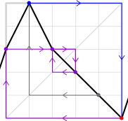
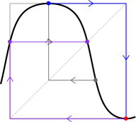
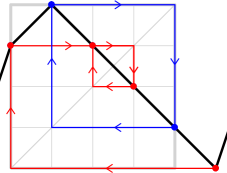
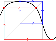
Figure 21: Piecewise linear model and the limiting lifted map for two weakly obstructed maps. On the left is shown a map with combinatorics ${(\!(}3,\,5,\,3,\,2,\,1,\,0{)\!)}$ and with the mapping pattern $x_{4}\mapsto\underline{\underline{x_{1}}}\mapsto\underline{\underline{x_{5}}}\mapsto x_{0}\mapsto x_{3}\leftrightarrow x_{2}~{}.$ On the right, a strictly unimodal map with combinatorics ${(\!(}3,\,4,\,3,\,2,\,1,\,0{)\!)}$ and mapping pattern $\underline{\underline{x_{5}}}\mapsto x_{0}\mapsto x_{3}\leftrightarrow x_{2}$ and $\underline{\underline{x_{1}}}\leftrightarrow x_{4}$.

Definition .

An obstruction will be called weak if the rational maps $f_{j}$ constructed during the iterated pull-back transformation converge locally uniformly to a critically finite map (but with simplified combinatorics, as defined in Section 2). Compare Figures 5 and 21. This can never happen if we start out with minimal combinatorics. (In the analogous case of polynomial maps, it follows from Selinger [S, Prop. 6.2] that weak obstructions are the only kind which can occur; but this is far from true for quadratic rational maps.)

The obstruction will be called strong if the fixed point multipliers $\mu_{j}$ converge to $\pm\infty$. Every combinatorics of $-+-$ bimodal shape is strongly obstructed (compare Section 3); and there are many strongly obstructed examples of $+-+$ shape (see Appendix A). On the other hand, for unimodal combinatorics we will show in Section 8 that there cannot be any strong obstruction except possibly in the totally non-hyperbolic case.

Note that $\mu_{j}$ always converges to $+\infty$ in the $-+-$ case, and to $-\infty$ in the $+-+$ obstructed case.

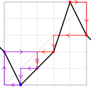
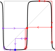
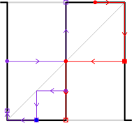
Figure 22: Piecewise linear model (left) and limiting lifted map (right) for the strongly obstructed combinatorics ${(\!(}2,\,0,\,1,\,2,\,5,\,3{)\!)}$. In the center is shown the result after two pullbacks. Of course what is actually shown on the right represents the quadratic map for some high iterate of the Thurston pull-back. Since these iterates are “trying” to duplicate combinatorics which cannot be realized, the pullback can never approximate the required dynamics. As in Figure 11 of Section 4, the image of a marked point $t_{j}$ under $F_{\ell}$ is indicated by an open square. In this example, the marked points $t_{2}$ and $t_{3}$ become arbitrarily close together while their images under the combinatorics ($t_{1}$ and $t_{2}$) remain distinct.

If we consider the ideal boundary of moduli space, as described in Section 6, then empirically, in all strongly obstructed cases, the following seems to be true. Either:

1. the combinatorics is $~{}+-+~{}$ bimodal, and the conjugacy classes $\langle f_{j}\rangle$ converge to the center point $(\Sigma,\,\Delta)=(-0.5,\,1)$ of ideal boundary of the $~{}+-+~{}$ region, or

2. the combinatorics is $~{}-+-~{}$ bimodal, and the conjugacy classes converge to the corresponding center point $(+0.5,\,1)$ for the $~{}-+-~{}$ region.

\begin{overpic}[height=173.44534pt]{newOz1-crop.pdf} \put(10.0,165.0){\rm SL} \put(160.0,165.0){\rm SL} \end{overpic}

\begin{overpic}[height=173.44534pt]{pmp-topOzm-crop.pdf} \put(10.0,165.0){\rm SL} \put(160.0,165.0){\rm SL} \end{overpic}

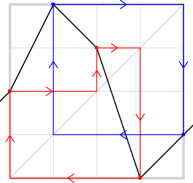
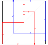
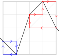
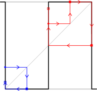
Figure 47: On the left are shown the piecewise linear map and limiting graph for the obstructed combinatorics ${(\!(}2,\,4,\,3,\,0,\,1{)\!)}$ of topological shape $+-+$ , with mapping pattern $\underline{\underline{x_{1}}}\leftrightarrow x_{4}$, $\underline{\underline{x_{3}}}\mapsto x_{0}\mapsto x_{2}\mapsto\underline{\underline{x_{3}}}$. On the right is the “left-right reflected version” with combinatorics ${(\!(}1,\,0,\,3,\,4,\,2{)\!)}$, topological shape $-+-$  and mapping pattern $\underline{\underline{x_{1}}}\leftrightarrow x_{0}$, $\underline{\underline{x_{3}}}\mapsto x_{4}\mapsto x_{2}\mapsto\underline{\underline{x_{3}}}$ .

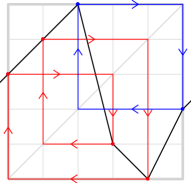
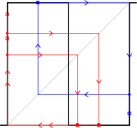
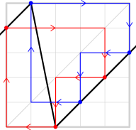
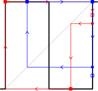
Figure 48: On the left is shown obstructed combinatorics ${(\!(}3,\,4,\,5,\,1,\,0,\,2{)\!)}$, with mapping pattern $\underline{\underline{x_{4}}}\mapsto x_{0}\mapsto x_{3}\mapsto x_{1}\mapsto\underline{\underline{x_{4}}}$ and $\underline{\underline{x_{2}}}\leftrightarrow x_{5}$. On the right is shown obstructed combinatorics ${(\!(}4,\,5,\,0,\,1,\,2,\,3{)\!)}$ with mapping pattern $\underline{\underline{x_{2}}}\mapsto x_{0}\mapsto x_{4}\mapsto{x_{2}}$ and $\underline{\underline{x_{1}}}\mapsto x_{5}\mapsto x_{3}\mapsto\underline{\underline{x_{1}}}$. Both have shape $+-+$.

${(\!(}2,3,4,6,4,0,1{)\!)}$	${(\!(}2,4,3,0,1{)\!)}$	${(\!(}3,5,4,0,1,2{)\!)}$	${(\!(}4,5,0,1,2,3{)\!)}$
$\kappa=-\infty$	$\kappa=-1$	$\kappa=(\sqrt{5}-1)/2$	$\kappa=+\infty$
	(Figure 47L)		(Figure 48R)

Figure 23: These images illustrate the convergence of four obstructed maps of topological shape $+-+$ toward the point $(\Sigma,\Delta)=(-0.5,\,1)$ in moduli space (see Section 6). Each colored broken line indicates $(\Sigma,\,\Delta)$ for consecutive steps of the pull-back; while the black curve is ${\bf Per}_{1}(1)$ which is the lower boundary of the shift locus (abbreviated as SL) in this region. The left half of this figure shows the window $(\Sigma,\,\Delta)\in[.8,1.2]\times[.95,1)$ with the vertical scale exaggerated by a factor of 8. The right half corresponds to the much smaller window $[.95,\,1.05]\times[.998,\,1)$ (indicated in dotted lines on the left), with the vertical scale exaggerated by a factor of 50. Observe that the green line enters the shift locus several times before converging to the point $(-0.5,\,1)$ in moduli space. The last line lists the conjectured limiting value of $\kappa$ as we converge to this ideal point.

\begin{overpic}[height=173.44534pt]{mpm-fig2-crop.pdf} \put(20.0,165.0){\rm SL} \put(160.0,165.0){\rm SL} \end{overpic}

\begin{overpic}[height=173.44534pt]{mpm-zfig2-crop.pdf} \put(10.0,165.0){\rm SL} \put(160.0,165.0){\rm SL} \end{overpic}

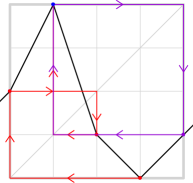
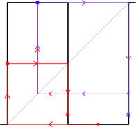
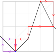
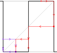
Figure 45: On the left an illustration of a strongly obstructed capture case with combinatorics ${(\!(}2,\,4,\,1,\,0,\,1{)\!)}$, topological shape $+-+$ , and mapping pattern $\underline{\underline{x_{3}}}\mapsto x_{0}\mapsto x_{2}\mapsto\underline{\underline{x_{1}}}\leftrightarrow x_{4}$. On the right, the “left-right reflected” version of the figure on the left, of topological shape $-+-$ with very similar dynamics, and very similar parameters. Like the figure on the left, it is the illustration of a strongly obstructed period two capture component. The combinatorics is ${(\!(}1,\,0,\,1,\,4,\,2{)\!)}$ and the mapping pattern is $\underline{\underline{x_{3}}}\mapsto x_{4}\mapsto x_{2}\mapsto\underline{\underline{x_{1}}}\leftrightarrow x_{0}$.

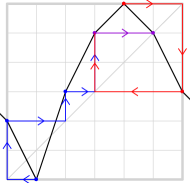
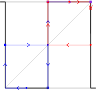
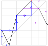
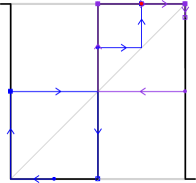
Figure 51: Two cases of shape $-+-$. Left: combinatorics ${(\!(}2,\,0,\,3,\,5,\,6,\,5,\,3{)\!)}$ and mapping pattern $\underline{\underline{x_{1}}}\mapsto x_{0}\mapsto x_{2}\mapsto x_{3}\mapsto x_{5}\,\rotatebox[origin={c}]{90.0}{\large$\circlearrowleft$}\,$ and $\underline{\underline{x_{4}}}\mapsto x_{6}\mapsto x_{3}\mapsto x_{5}\,\rotatebox[origin={c}]{90.0}{\large$\circlearrowleft$}\,$. Right: combinatorics ${(\!(}2,\,0,\,4,\,5,\,6,\,5,\,3{)\!)}$ and mapping pattern $\underline{\underline{x_{1}}}\mapsto x_{0}\mapsto x_{2}\mapsto\underline{\underline{x_{4}}}\mapsto x_{6}\mapsto x_{3}\mapsto x_{5}\,\rotatebox[origin={c}]{90.0}{\large$\circlearrowleft$}\,$.

${(\!(}2,0,3,5,6,5,3{)\!)}$	${(\!(}1,0,3,2{)\!)}$	${(\!(}1,0,3,4,2{)\!)}$	${(\!(}1,0,1,4,2{)\!)}$
$\kappa=+1$	$\kappa=0$	$\kappa=-1$	$\kappa=-1$
(Figure 51L)			(Figure 45R)

Figure 24: This image illustrates the convergence of four obstructed maps of topological shape $-+-$ toward the point $(\Sigma,\Delta)=(0.5,\,1)$ in moduli space (see Section 6). Each colored broken line indicates $(\Sigma,\,\Delta)$ for successive steps of the pull-back. The Chebyshev curve $|\kappa|=1$, shown in gray, is the lower boundary of the shift locus $|\kappa|>1$ in this region. It satisfies $\Delta\,=\,1-|\Sigma-.5|+{\mathcal{O}}\big{(}(\Sigma-.5)^{2}\big{)}$; see Section 6. The figure on the left shows the window $(\Sigma,\,\Delta)\in[.9,\,1.1]\times[.8,\,1)$. The figure on the right is a zoom of the upper left by a factor of 15. Note that both the red and the blue curves seem to stay inside the shift locus while converging to the ideal point $(\Sigma,\Delta)=(0.5,\,1)$; but that the yellow and green curves remain outside the shift locus while converging to the same point. (In fact the green curve is contained in the line $\Sigma=.5$.) Near $(0.5,1)$, the blue and the yellow curves get extremely close to the boundary of the shift locus. Again the conjectured limiting values of $\kappa$ are indicated.

It is interesting that $(\Sigma,\,\Delta)=(\pm.5,~{}1)$ are the only two points in the upper ideal boundary which can be approximated by conjugacy classes which are not in the shift locus. (Compare Figure 17.)

Conjecture .

For any admissible combinatorics, either one or both of the following two conditions must hold:

1. at most finitely many of the successive conjugacy classes generated by the Thurston algorithm belong to the shift locus, and/or

2. the successive conjugacy classes converge to one of the two ideal points with coordinates $(\Sigma,\,\Delta)=(\pm.5,~{}1)$.

Clearly (a) must be satisfied in the unobstructed case. However, Figures 45R and 51L illustrate an obstructed case of shape $-+-$ where the successive conjugacy classes appear to converge to $(.5,\,1)$ through the shift locus. Figure 23 illustrates an obstructed case of shape $+-+$ where the successive conjugacy classes enter the shift locus at least three times.

In Case (b), the direction of approach to the ideal point depends of the limiting behavior of the Epstein parameter $\kappa$. (Compare Section 6.) In many strongly obstructed cases, $\kappa$ tends to a finite limit, and the convergence seems quite orderly. However there are also cases where the convergence is much wilder, and this is particularly true in cases where $\kappa$ tends to infinity. Various possibilities are illustrated in Figure 23.

Clearly Section 7 would have the following consequence.

Conjecture .

For strongly obstructed combinatorics, the only possible limit is $(-.5,\,1)$ in the $+-+$ case, or $(+.5,\,1)$ in the $-+-$ case. But in the unimodal case, every minimal combinatorics is unobstructed.

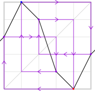
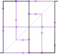
Figure 44: The piecewise linear map and the the limit of the iterated pull-back maps are shown for the strongly obstructed combinatorics ${(\!(}3,\,5,\,4,\,1,\,0,\,2{)\!)}$ of topological shape $+-+$  and mapping pattern $\underline{\underline{x_{4}}}\mapsto x_{0}\mapsto x_{3}\mapsto\underline{\underline{x_{1}}}\mapsto x_{5}\mapsto x_{2}\mapsto\underline{\underline{x_{4}}}$ .

For a strongly obstructed case the lifted form of the limit map will be a square wave; as illustrated in Figure 22 in the $~{}-+-~{}$ case, or as illustrated in Figure 44 in the $~{}+-+~{}$ case. (See also Figures 45, 47, 48.)

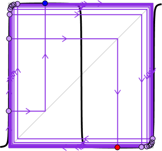
Figure 25: This figure is the graph of a Filom-Pilgrim map of class ${\rm FP}(8,\,9)$. (Compare Section 6.) This is an honest smooth critically finite rational map of Type B and shape $+-+$. However it is so close to the ideal point $(\Sigma,\Delta)=(-.5,\,,1)$ of moduli space, that its graph looks very much like the graph of an obstructed map.

Caution. One can’t be sure by looking at a graph that the combinatorics is obstructed. In fact any critically finite conjugacy class which is sufficiently close to the ideal boundary will have a graph which cannot be distinguished from a square wave. See Figure 25.

Constructing Levy Cycles

Every combinatorics ${\stackrel{{\scriptstyle\rightarrow}}{{m}}}={(\!(}m_{0},\cdots,m_{n}{)\!)}$ gives rise to a corresponding Markov partition of the interval $[0,n]$ into $n$ subintervals $I(j)=[j-1,~{}j]$. The associated piecewise linear map ${\bf f}$ sends each $I(j)$ linearly onto some union of one or more consecutive subintervals. By a periodic orbit of period $p$ for the associated Markov shift we will mean a list of $p$ of these $I(j)$, indexed by integers $k$ modulo $p$, and satisfying the condition that

$${\bf f}\big{(}I(j_{k})\big{)}~{}\supset~{}I(j_{k+1})$$

for each $k$.

Theorem .

Let ${\stackrel{{\scriptstyle\rightarrow}}{{m}}}$ be an admissible combinatorics of shape $+-+$. If there exists a periodic orbit $\{I(j_{k})\}$ of period $p\geq 2$ for the associated Markov shift which satisfies the following three conditions, then there is a Levy cycle, and hence the combinatorics is strongly obstructed.

1. Every $I(j_{k})$ is contained in an increasing lap of ${\bf f}$.

2. These intervals $I(j_{k})$ are disjoint: In particular, no two have a common end point.

3. If we think of $[0,~{}n]$ as a subset of the circle ${\widehat{\mathbb{R}}}$, then the correspondence $I(j_{k})\to I(j_{k+1})$ has a well defined rotation number. In particular, this correspondence preserves the cyclic order of the intervals $I(j_{k})$ within ${\widehat{\mathbb{R}}}$.

Remark .

Here any period $p\geq 2$ can actually occur. Consider the combinatorics ${(\!(}2,\,3,\,4,\,5,\,\ldots,\,n-1,\,n,\,0,\,1{)\!)}$. If $n$ is odd, then this combinatorics has Type D, and it is not hard to check that

$${\bf f}:I(1)\stackrel{{\scriptstyle\cong}}{{\longrightarrow}}I(3)\stackrel{{\scriptstyle\cong}}{{\longrightarrow}}I(5)\stackrel{{\scriptstyle\cong}}{{\longrightarrow}}\cdots\stackrel{{\scriptstyle\cong}}{{\longrightarrow}}I(n)\stackrel{{\scriptstyle\cong}}{{\longrightarrow}}I(1)~{},$$

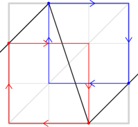
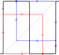
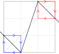
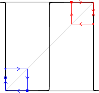
Figure 46: On the left are illustrations of a piecewise linear map and limiting graph of a map of topological shape $+-+$  with combinatorics ${(\!(}2,\,3,\,0,\,1{)\!)}$, mapping pattern $\underline{\underline{x_{2}}}\leftrightarrow x_{0}$, $\underline{\underline{x_{1}}}\leftrightarrow x_{3}$. On the right is the “left-right reflected version” which is of topological shape $-+-$  with combinatorics ${(\!(}1,\,0,\,3,\,2{)\!)}$ and mapping pattern $\underline{\underline{x_{1}}}\leftrightarrow x_{0}$, $\underline{\underline{x_{2}}}\leftrightarrow x_{3}$.

with period $p=(n+1)/2$. Thus there is a Levy cycle, and the combinatorics is strongly obstructed. See Figures 46L and 48R for the cases ${(\!(}2,3,0,1{)\!)}$ and (​(4,5,0,1,2,3)​).

Remark .

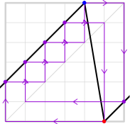
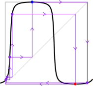
Figure 37: An illustration of the piecewise linear map and its corresponding rational map for the combinatorics ${(\!(}2,\,3,\,4,\,5,\,6,\,0,1{)\!)}$ with shape $~{}+-+~{}$ and mapping pattern $\underline{\underline{x_{5}}}\mapsto x_{0}\mapsto x_{2}\mapsto\underline{\underline{x_{4}}}\mapsto x_{6}\mapsto x_{1}\mapsto x_{3}\mapsto\underline{\underline{x_{5}}}$ .

On the other hand, for $n$ even the combinatorics is of Type B, and is always unobstructed. In fact, in the notation of Section 6, these are just the Filom-Pilgrim conjugacy classes of the form ${\langle}f_{2,\,q}{\rangle}$, with $q>2$ odd. In Figure 19, these are the orange dots in the left half of the figure (for $q\geq 5$), together with one red dot on the right corresponding to ${\langle}f_{2,3}{\rangle}$. (See Figure 36R for the case $q=5$ and Figure 37 for the case $q=7$ .)

We will first prove Section 7 for the case $p=2$, and then for $p>2$. The first step for any period $p$ is to consider the interval $[0,n]$ as a subset of ${\widehat{\mathbb{R}}}$, which we think of as the equator of the Riemann sphere $\widehat{\mathbb{C}}$. (Compare Figure 3.) Then extend the piecewise linear map on $[0,\,n]$ to a Thurston map ${\bf f}:\widehat{\mathbb{C}}\to\widehat{\mathbb{C}}$ as described in Section 2.

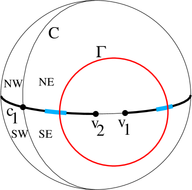
Figure 26: A picture of the Riemann sphere, illustrating the case $p=2$. Here ${\widehat{\mathbb{R}}}$ is represented as the equator, and the pure imaginary axis is represented as an orthogonal great circle which intersects the equator at the two critical points. The Thurston map ${\bf f}$ sends ${\widehat{\mathbb{R}}}$ two-to-one onto ${\bf f}({\widehat{\mathbb{R}}})$, which is colored heavy black, except for the two intervals $I(j_{0})$ and $I(j_{1})$ which are blue. The great circle $C$ maps two-to-one onto the gap ${\widehat{\mathbb{R}}}{\smallsetminus}{\bf f}({\widehat{\mathbb{R}}})$ between the two critical values. The Levy cycle $\Gamma$, which is colored red, passes through $I(j_{0})$ and $I(j_{1})$. It is important that $\Gamma$ does not separate the two critical values, or the two critical points. Note that the northeast and southwest quadrants both map bijectively onto the northern hemisphere under ${\bf f}$, while the northwest and southeast quadrants both map bijectively onto the southern hemisphere.

Proof of Section 7 for the case $p=2$.

In this case, we have two intervals with

$${\bf f}\big{(}I(j_{0})\big{)}\supset I(j_{1})\quad{\rm and}\quad{\bf f}\big{(}I(j_{1})\big{)}\supset I(j_{0})~{}.$$

(Compare Figure 26.) Therefore there exist interior points $r\in I(j_{0})$ and $s\in I(j_{1})$ which map respectively to interior points $r^{\prime}\in I(j_{1})$ and $s^{\prime}\in I(j_{0})$. Our Levy cycle will consist of a single simple closed curve $\Gamma$ which is the union of:

1. a path from $r^{\prime}$ to $s^{\prime}$ lying in the northeast quadrant, above the equator and to the right of $C$,

2. the image of this path under complex conjugation, which lies in the southeast quadrant.

It is not hard to check that the set ${\bf f}^{-1}(\Gamma)$ has two connected components. One also lies in the eastern hemisphere, and is homotopic to $\Gamma$ within the complement of the postcritical set, as required. The other component lies in the western hemisphere, and can be ignored. This completes the proof in the period two case. ∎

Here is a corollary to the period two case.

Corollary .

Every admissible combinatorics of shape $+-+$ with a period two critical orbit is strongly obstructed.

Proof.

Let $v_{1}<c_{2}<c_{1}<v_{2}$ be the critical points and corresponding critical values; and suppose for example that $c_{2}\leftrightarrow v_{2}$ is the period two critical orbit. Let $I_{j}$ be the last interval in the first lap, with right hand endpoint $c_{2}$; and let $I_{n}$ be the last subinterval, with right hand endpoint $v_{2}$. Since $c_{2}\leftrightarrow v_{2}$ it is easy to check that $F(I_{j})\subset I_{n}$ and that $F(I_{n})\supset I_{j}$. The conclusion follows. ∎

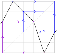
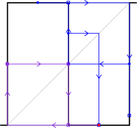
Figure 50: An illustration of a strongly obstructed map of topological shape $+-+$  with combinatorics ${(\!(}3,\,5,\,4,\,3,\,0,\,2{)\!)}$ and mapping pattern $\underline{\underline{x_{1}}}\mapsto x_{5}\mapsto x_{2}\mapsto\underline{\underline{x_{4}}}\mapsto x_{0}\mapsto x_{3}\,\rotatebox[origin={c}]{90.0}{\large$\circlearrowleft$}\,$.

As examples, see Figures 45(left), 46(left), 47(left), 48(left), and 49(left). There are also examples with a period two orbit for the Markov shift but with no period two critical orbit. Consider Figure 44, with combinatorics ${(\!(}3,5,4,1,0,2{)\!)}$ of Type B. In this case it is not hard to check that $F(I_{1})\supset I_{5}$ and that $F(I_{5})\supset I_{1}$. Hence again it follows that the combinatorics is strongly obstructed. There are even examples with no periodic critical orbit of any period. See Figure 50, a totally non-hyperbolic map with combinatorics ${(\!(}3,5,4,3,0,2{)\!)}$, also satisfying $F(I_{1})\supset I_{5}$ and $F(I_{5})\supset I_{1}$, and hence also strongly obstructed.

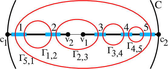
Figure 27: A neighborhood of the increasing half-circle within the eastern hemisphere of the Riemann sphere, illustrating a Levy cycle of period $p=5$. The blue line segments represent the periodic intervals, numbered from left to right by the numbers one through $p$. For any $p$ there must be at least one and at most $p-1$ such intervals in the increasing lap $[c_{1},~{}v_{2}]$, with the remaining periodic intervals in the other increasing lap $[v_{1},~{}c_{2}]$. The loops $\Gamma_{i,j}$ of the Levy cycle are numbered according to the intervals where they cross the real axis (= equator).

Proof of Section 7 for the case $p>2$.

To simplify the notation, we will simply label the $p$ periodic intervals $I(j_{k})$ by integers from one to $p$ in positive cyclic order within the increasing half-circle. If the rotation number is $m/p$, then the image of interval $j$ under the Thurston map ${\bf f}$ will contain interval with number $j+m~{}~{}({\rm mod}~{}p)$. Thus we can choose two points $r_{j}<s_{j}$ in each interval $j$ with images $r^{\prime}_{j+m}<s^{\prime}_{j+m}$ in the interior of interval $j+m$. Now join each $s^{\prime}_{j}$ to $r^{\prime}_{j+1}$ by a path within the northern hemisphere and also by the conjugate path within the southern hemisphere. The result will be a loop $\Gamma_{j,\,j+1}$. It is always possible to do this so that the loops are disjoint, and contained in the eastern hemisphere, as illustrated in Figure 27. Furthermore, it is not hard to see that there is a branch of ${\bf f}^{-1}$ which carries each $\Gamma_{j,\,j+1}$ to a loop which is homotopic to $\Gamma_{j-m,\,j+1-m}$ within $\widehat{\mathbb{C}}{\smallsetminus}P$, where $P$ is the postcritical set. This completes the proof of Section 7. ∎

8 Unimodal Maps

Let ${\mathcal{U}}$ be the open unimodal region of ${\mathcal{M}}/{\mathcal{I}}$ (see Figure 17), and let $\overline{\mathcal{U}}$ be its topological closure, consisting not only of unimodal classes but also of polynomial and co-polynomial classes. In this section, we will always choose the orientation so the the maps have shape $-+$. Thus for all ${\langle}f{\rangle}$ in $\overline{\mathcal{U}}$ there is a primary critical point $c_{1}$ where $f$ takes its minimum value, and a secondary critical point $c_{2}$ where $f$ takes its maximum value. If ${\langle}f{\rangle}$ belongs to the open set ${\mathcal{U}}$, then the critical point $c_{1}$ is in the interior of $f({\widehat{\mathbb{R}}})$ while $c_{2}$ is in the complement of $f({\widehat{\mathbb{R}}})$.

Bones

By definition, a bone in $\overline{\mathcal{U}}$ is a connected component of the locus of ${\langle}f{\rangle}$ for which the primary critical point $c_{1}$ is periodic, with some specified period $p\geq 2$ and specified order type. Filom [F], making use of Kiwi and Rees [KR], shows that every bone in $\overline{\mathcal{U}}$ is a smooth manifold, which is either a bone-arc, diffeomorphic to a closed interval, or a bone-loop, diffeomorphic to a circle. He proves the following. (See [F, 6.2].)

Lemma .

Every bone-arc in $\overline{\mathcal{U}}$ has one endpoint in the polynomial boundary and one endpoint in the co-polynomial boundary. Furthermore, for every polynomial or co-polynomial class for which $c_{1}$ is periodic of period $p\geq 2$, there is a corresponding bone-arc.

We can understand this statement on a purely combinatorial level as follows.

Proposition .

There is a natural one-to-one correspondence between combinatorics ${(\!(}m_{0},\ldots,m_{n}{)\!)}$ of polynomial shape and combinatorics ${(\!(}m_{0},\ldots,m_{n-1}{)\!)}$ of co-polynomial shape, except in two extreme cases: For the polynomial combinatorics ${(\!(}2,0,2{)\!)}$, corresponding to the Chebyshev map $f(x)=x^{2}-2$, and the polynomial combinatorics ${(\!(}0,1{)\!)}$ corresponding to $f(x)=x^{2}$, there is no corresponding co-polynomial combinatorics.

Proof.

After reversing orientation if necessary, we may assume that both combinatorics are of $-+$ shape. Thus the critical fixed point in the polynomial case (corresponding to the point at infinity for an actual polynomial) will be to the right. Then the polynomial combinatorics takes the form ${(\!(}m_{0},m_{1},\ldots,m_{n-1},n{)\!)}$. By definition, the associated co-polynomial combinatorics ${\stackrel{{\scriptstyle\rightarrow}}{{m}}}={(\!(}m_{0},m_{1},\ldots,m_{n-1}{)\!)}$ is obtained simply by deleting the last entry $m_{n}=n$. If we exclude the Chebyshev case and the ${(\!(}0,1{)\!)}$ case, then it is not hard to check that this resulting ${\stackrel{{\scriptstyle\rightarrow}}{{m}}}$ does indeed have co-polynomial shape. Similarly it is not hard to check that every ${\stackrel{{\scriptstyle\rightarrow}}{{m}}}$ of co-polynomial shape can be uniquely augmented to obtain a combinatorics of polynomial shape. ∎

For a typical hyperbolic example see Figure 28, while for a typical non-hyperbolic example see Figure 29.

   

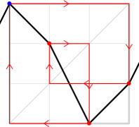
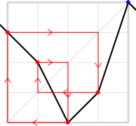
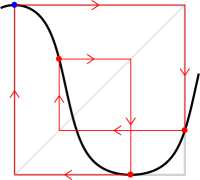
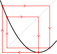
Figure 28: On the left, the combinatorics ${(\!(}3,2,0,1{)\!)}$ has co-polynomial shape. with mapping pattern $\underline{\underline{x_{2}}}\mapsto\underline{\underline{x_{0}}}\mapsto x_{3}\mapsto x_{1}\mapsto\underline{\underline{x_{2}}}$. Next to it, the corresponding polynomial combinatorics ${(\!(}3,2,0,1,4{)\!)}$, with mapping pattern $\underline{\underline{x_{2}}}\mapsto x_{0}\mapsto x_{3}\mapsto x_{1}\mapsto\underline{\underline{x_{2}}}$ together with $\underline{\underline{x_{4}}}\,\rotatebox[origin={c}]{90.0}{\large$\circlearrowleft$}\,$. Note that $x_{0}$ is a critical point for the co-polynomial shape, but not for the polynomial shape. On the right center, the lifted rational map for the co-polynomial combinatorics with $\mu=-3.79681$ and $\kappa=0.898403$. To the right of it, the corresponding polynomial map $f(x)=x^{2}-1.3107\cdots$ with combinatorics ${(\!(}3,2,0,1,4{)\!)}$.

   

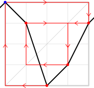
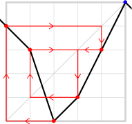
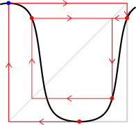
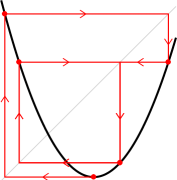
Figure 29: A non-hyperbolic example. First on the left, co-polynomial combinatorics ${(\!(}4,3,0,1,3{)\!)}$ with mapping pattern $\underline{\underline{x_{2}}}\mapsto\underline{\underline{x_{0}}}\mapsto x_{4}\mapsto x_{3}\leftrightarrow x_{1}$. Next to it, the corresponding polynomial combinatorics ${(\!(}4,3,0,1,3,5{)\!)}$ with mapping pattern $\underline{\underline{x_{2}}}\mapsto x_{0}\mapsto x_{4}\mapsto x_{3}\leftrightarrow x_{1}$ and $\underline{\underline{x_{5}}}\,\rotatebox[origin={c}]{90.0}{\large$\circlearrowleft$}\,$. Note that $\underline{\underline{x_{0}}}$ is a critical point on the left but not on the right. The right center shows the lifted map for the co-polynomial combinatorics ${(\!(}4,3,0,1,3{)\!)}$ with $\mu=-5.53846$ and $\kappa=1.76923$. To the right of it is the graph of the corresponding polynomial $f(x)=x^{2}-1.839287$.

Thus, the correspondence between critically finite polynomial dynamics and co-polynomial dynamics works just as well in the non-hyperbolic case. This suggests the following definition and conjecture.

Definition .

By a “non-hyperbolic bone”, or briefly NH-bone, in $\overline{\mathcal{U}}$ we will mean a connected component of the locus of points for which $c_{1}$ is eventually periodic repelling, with specified eventual period $p\geq 1$ and pre-period $q\geq 2$. (Here by the “pre-period” we mean the smallest $q$ for which $f^{\circ q}(c_{1})$ is periodic.)

Conjecture .

Such NH-bones behave very much like the usual bones. In particular they are smooth manifolds and (with one exception) every NH-bone-arc joins a point on the polynomial locus to a point on the co-polynomial locus. The unique exception is the “Chebyshev” NH-bone, which starts on the polynomial locus at $\langle x\mapsto x^{2}-2\rangle$, and forms part of the boundary of the shift locus until it hits ${\bf Per}_{1}(1)$ tangentially. (Compare Figure 17.) At this point the repelling fixed point becomes attracting. The analytically continued curve is contained in the shift locus and diverges towards the ideal boundary point without ever reaching the co-polynomial locus.

The ten simplest examples of the correspondence between co-polynomial combinatorics and polynomial combinatorics are shown in Table 8.0, and the ten corresponding bone-arcs or NH-bone-arcs are shown in Figure 30.

Kneading Numbers

Kneading theory is a useful tool for all piecewise monotone maps of the interval (compare [MTh]). However, in the unimodal case it can be described in a particularly simple and easy to use form.

For any $f$ with $\langle f\rangle\in\overline{\mathcal{U}}$ there is a dynamic kneading function

$${\bf k}~{}=~{}{\bf k}_{f}:f({\widehat{\mathbb{R}}})\to[-1,\,1]~{},$$

defined in two steps as follows. The image ${\bf k}(x)$ can be thought of as an invariantly defined coordinate for the point $x\in f({\widehat{\mathbb{R}}})$.

Definition .

For each $x\in f({\widehat{\mathbb{R}}})$ let:

$$\sigma(x)=\begin{cases}\mbox{\quad}0\quad{\rm if}\quad x\quad{\rm is\;\,equal\;\,to\;\,the\,\;primary\;\,critical\;\,point}\;\,c_{1}~{},\\ \mbox{\quad}1\quad{\rm if}\quad x\quad{\rm is\;\,in\;\,the\;\,increasing\;\,lap}~{},\\ -1\quad{\rm if}\quad x\quad{\rm is\,\;in\;\,the\;\,decreasing\;\,lap}~{}.\end{cases}$$

Note that $\sigma(x)$ can be identified with the sign of the derivative $f^{\prime}(x)$, except in the case of a pole, with $f(x)=\infty$. (Of course if $f({\widehat{\mathbb{R}}})\subset{\mathbb{R}}$, then there are no poles.) Now for any $x_{0}\in f({\widehat{\mathbb{R}}})$ with orbit $~{}~{}f:x_{0}\mapsto x_{1}\mapsto\cdots$,   define

$${\bf k}(x_{0})~{}=~{}\sum_{h\geq 0}\frac{\sigma(x_{0})\sigma(x_{1})\cdots\sigma(x_{h})}{2^{h+1}}~{}.$$

Table 8.0: Examples of co-polynomial maps, showing the kneading invariant as defined below, and listing the corresponding $c$ values for $f_{c}(x)=x^{2}-c$ . The notation $B(p)$ means that both critical points are contained in a common orbit of period $p$.

$\stackrel{{\scriptstyle\hbox{{figure}}\rule{0.0pt}{9.64441pt}}}{{\hbox{{number}}\rule[-5.16663pt]{0.0pt}{0.0pt}}}$	$\stackrel{{\scriptstyle\hbox{{topological}}\rule{0.0pt}{9.64441pt}}}{{\hbox{{shape}}\rule[-5.16663pt]{0.0pt}{0.0pt}}}$	$\stackrel{{\scriptstyle\hbox{{co-polynomial}}\rule{0.0pt}{9.64441pt}}}{{\hbox{{combinatorics}}\rule[-5.16663pt]{0.0pt}{0.0pt}}}$	$\stackrel{{\scriptstyle\hbox{{dynamic}}\rule{0.0pt}{9.64441pt}}}{{\hbox{{type}}\rule[-5.16663pt]{0.0pt}{0.0pt}}}$	$\stackrel{{\scriptstyle\hbox{{kneading}}\rule{0.0pt}{9.64441pt}}}{{\hbox{{invariant}}\rule[-5.16663pt]{0.0pt}{0.0pt}}}$	$\stackrel{{\scriptstyle\hbox{{corresponding}}\rule{0.0pt}{9.64441pt}}}{{\hbox{{polynomial}}\rule[-5.16663pt]{0.0pt}{0.0pt}}}$
35L	$+\,-$	${(\!(}1,\,2,\,3,\,4,\,0{)\!)}$	$B(5)$
	$-\,+$	${(\!(}4,\,0,\,1,\,2,\,3{)\!)}$		0.9375	$c=1.985424253$
34L	$+\,-$	${(\!(}1,\,2,\,3,\,0{)\!)}$	$B(4)$
	$-\,+$	${(\!(}3,\,0,\,1,\,2{)\!)}$		0.875	$c=1.940799807$
43	$+\,-$	${(\!(}1,\,3,\,4,\,3,\,0{)\!)}$	$NH$
	$-\,+$	${(\!(}4,\,1,\,0,\,1,\,3{)\!)}$		0.833333	$c=1.892910988$
36L	$+\,-$	${(\!(}1,\,3,\,4,\,2,\,0{)\!)}$	$B(5)$
	$-\,+$	${(\!(}4,\,2,\,0,\,1,\,3{)\!)}$		0.8125	$c=1.860782522$
42R	$+\,-$	${(\!(}1,\,3,\,4,\,1,\,0{)\!)}$	$NH$
29	$-\,+$	${(\!(}4,\,3,\,0,\,1,\,3{)\!)}$		0.8	$c=1.839286755$
33R	$+\,-$	${(\!(}1,\,2,\,0{)\!)}$	$B(3)$
	$-\,+$	${(\!(}2,\,0,\,1{)\!)}$		0.75	$c=1.754877666$
35R	$+\,-$	${(\!(}2,\,4,\,3,\,1,\,0{)\!)}$	$B(5)$
	$-\,+$	${(\!(}4,\,3,\,1,\,0,\,2{)\!)}$		0.6875	$c=1.625413725$
42L	$+\,-$	${(\!(}2,\,3,\,2,\,0{)\!)}$	$NH$
	$-\,+$	${(\!(}3,\,1,\,0,\,1{)\!)}$		0.666667	$c=1.543689013$
34R	$+\,-$	${(\!(}2,\,3,\,1,\,0{)\!)}$	$B(4)$
28	$-\,+$	${(\!(}3,\,2,\,0,\,1{)\!)}$		0.625	$c=1.310702641$
33L	$-$	${(\!(}1,\,0{)\!)}$	$B(2)$	0.5	$c=1$

Lemma .

If $f$ has shape $-+$, then ${\bf k}(x)$ is a monotone increasing function. That is,

$$~{}~{}x<y~{}\Rightarrow~{}{\bf k}(x)\leq{\bf k}(y)~{}.$$

Similarly, in the $+-$ case it is monotone decreasing. This function ${\bf k}(x)$ is not continuous: It has a jump discontinuity at $c_{1}$ and at every iterated pre-image of $c_{1}$; but is continuous everywhere else.

Proof by contradiction.

First consider the $-+$ case so that

$$\sigma(x)<\sigma(y)\quad\longrightarrow\quad x<y~{}.$$

Let $x=x_{0}\mapsto x_{1}\cdots$ and $y=y_{0}\mapsto y_{1}\cdots$ be the orbits. If ${\bf k}(x)>{\bf k}(y)$, let $n$ be the smallest integer with $\sigma(x_{n})\neq\sigma(y_{n})$, and let

$$s=\prod_{0\leq j<n}\sigma(x_{j})=\prod_{0\leq j<n}\sigma(y_{j})~{}.$$

Then $s\,\sigma(x_{n})>s\,\sigma(y_{n})$, hence $s\,x_{n}>s\,y_{n}$. But $s$ is the sign of the derivative of $f^{\circ n}$ on the interval between $x$ and $y$, so it follows that $x>y$, contradicting our hypothesis. The $+-$ case is similar, and the rest of the proof is straightforward. ∎

Lemma .

If we are in the ${\mathscr{F}}(0,1)$ region of ${\mathcal{U}}$, with no attracting or parabolic fixed points, then the real number ${\bf k}(x_{0})$ completely determines the sequence of signs $\sigma(x_{j})$. In particular, it follows that the sign of ${\bf k}(x)$ is equal to $~{}\sigma(x)$.

Proof.

This could fail only if the sequence of signs $\sigma(x_{j})$ had the form $(\pm 1,\mp 1,1,1,1,\cdots)$ for some $x$, so that ${\bf k}(x)=\pm(1/2-1/4-1/8-\cdots)$ would be zero although the signs are all non-zero. But this would imply that the orbit of $x$ converges to an attracting or parabolic fixed point. ∎

For the two dimensional set $\overline{\mathcal{U}}$ we can define two invariant coordinates ${\bf K}_{1}$ and ${\bf K}_{2}$, each sending $\overline{\mathcal{U}}$ to $[-1,\,1]$. These kneading functions on moduli space are defined by the formula

$${\bf K}_{j}(f)~{}=~{}-{\bf k}_{f}(v_{j})\qquad{\rm where}\quad v_{j}\quad{\rm is~{}the~{}critical~{}value}\quad f(c_{j})~{}.$$

Here the minus sign is inserted for convenience, so that we will have ${\bf K}_{1}(f)\geq 0$ in dynamically interesting cases (although ${\bf K}_{2}(f)\leq 0$). It is not hard to check that ${\bf K}_{1}(f)$ is constant along each bone, and serves to distinguish one bone from another (provided that there are no bone-loops). On the other hand, ${\bf K}_{2}(f)$ can be thought of as an invariantly defined coordinate along each bone. Note that the definition of ${\bf K}_{1}(f)$ ignores the critical points $c_{2}$, while definition of ${\bf K}_{2}(f)$ involves the interplay between the orbits of $c_{1}$ and $c_{2}$.

Evidently ${\bf K}_{1}(f)$ is a sum of only finitely many terms if and only if the critical point $c_{1}$ is periodic, so that $f$ belongs to a bone. In this case, ${\bf K}_{1}(f)$ will jump discontinuously under perturbation of $f$. However, whenever the critical point $c_{1}$ is not periodic, ${\bf K}_{1}(f)$ will vary continuously. Note also that ${\bf K}_{1}(f)$ is a rational number whenever $f$ belongs either to a bone or to an NH-bone. (Compare Table 8.0.)

Lemma .

Every critically finite map $f$ is uniquely determined up to $\pm$-conjugacy by the pair of rational numbers $\big{(}{\bf K}_{1}(f),\,{\bf K}_{2}(f)\big{)}$.

Proof.

It follows from Section 8 that the order of the points in the orbit of $c_{1}$ is determined by ${\bf K}_{1}(f)$, and the relative position of the orbit of $v_{2}$ is then determined by ${\bf K}_{2}(f)$. Thus the combinatorics is uniquely determined; and the conclusion follows from Section 5.∎

Some typical examples of level sets of ${\bf K}_{1}$ are shown in Figure 30. The level sets of ${\bf K}_{2}$ are more complicated. (See Figure 31.)

\begin{overpic}[width=216.81pt]{knpic3bw.png} \put(100.0,75.0){${\mathcal{U}}$} \end{overpic}

Figure 30: Illustrating ten bone-arcs or NH-bone-arcs joining a co-polynomial on the left to a polynomial on the right, corresponding to the ten cases listed in Table 8.0. Here, as in Figures 17 and 32, the space ${\mathcal{U}}$ of unimodal conjugacy classes is represented by a right-angled rhombus. This figure is closely related to the plot of topological entropy in Figure 32.

  

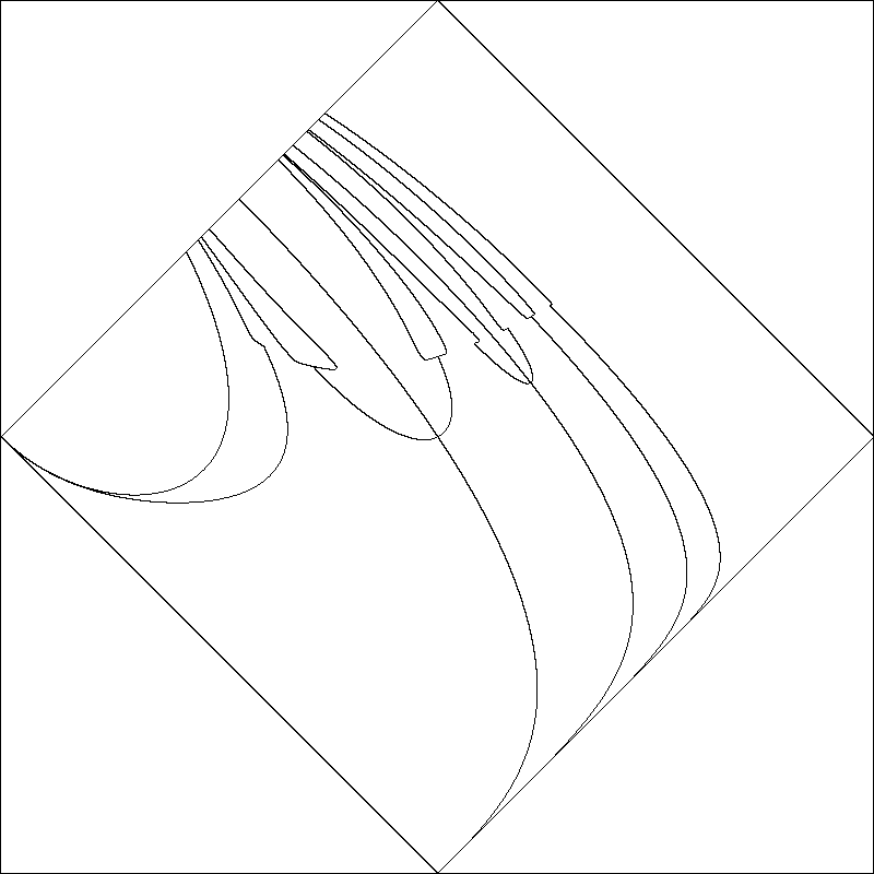
Figure 31: The region ${\mathcal{U}}$ divided into fourteen colored regions according to the value of ${\bf K}_{2}(f)$. On the right, the boundaries between these regions.

Here is simple application of kneading.

Lemma .

Minimal co-polynomial combinatorics are unobstructed in all cases.

Proof.

As we traverse the one-parameter family of polynomials, we encounter every possible critically finite kneading sequence. (See [MTh, Thm. 12.2].) But as we follow the one parameter family of co-polynomials

$$f(x)=1/(x^{2}+c)\,,$$

it follows from Section 8 that we encounter exactly the same critically finite kneading sequences. Thus every minimal admissible co-polynomial combinatorics is realized by an actual co-polynomial, and there is no obstruction. ∎

Making use of Filom’s proof that each bone-arc in $\overline{\mathcal{U}}$ terminates at a co-polynomial at one end and a polynomial at the other end, we have the following.

Theorem .

The function ${\bf K}_{1}(f)$ is constant along each bone-arc; while the function ${\bf K}_{2}(f)$ is monotone increasing as we follow each bone-arc from its polynomial endpoint to its co-polynomial endpoint.

Proof.

The first statement is clear. For the second statement, note that we need only consider the upper half of the polynomial boundary (corresponding to conjugacy classes of the form $\langle x\mapsto x^{2}+v_{1}\rangle$ with $v_{1}<0$), since the lower half does not have any critically finite points. For ${\langle}f{\rangle}$ in the upper half of the polynomial boundary, the critical point $c_{2}$ is fixed, so that ${\bf K}_{2}(f)=-1$. As $f$ varies along a bone, note that the correspondence $f\mapsto{\bf K}_{2}(f)$ can change its value only when the orbit of $c_{2}$ passes through $c_{1}$, which means that we pass through a critically finite capture configuration. Furthermore each such capture combinatorics can occur only once, since a critically finite map is determined by its combinatorics. This proves that the map which sends each $f$ on the bone to ${\bf K}_{2}(f)\in[-1,1]$ is monotonic. ∎

Table 8.0: On the left, seven critically finite points along the bone-arc for which the critical point $c_{1}$ has period two. On the right, seven points along the bone-arc for which $c_{1}$ has period three. Note that the values of ${\bf K}_{2}$ are rational, with small denominators since $n$ is small.

${\bf K}_{1}=0.5$			${\bf K}_{1}=0.75$
shape	combinatorics	${\bf K}_{2}$	shape	combinatorics	${\bf K}_{2}$
polynomial (D)	${(\!(}1,0,2{)\!)}$	$-1$	polynomial (D)	${(\!(}2,0,1,3{)\!)}$	$-1$
unimodal (C)	${(\!(}7,2,1,2,3,4,5,6{)\!)}$	$-0.96875$	unimodal (C)	${(\!(}7,3,1,2,3,4,5,6{)\!)}$	$-0.96875$
unimodal (C)	${(\!(}6,2,1,2,3,4,5{)\!)}$	$-0.9375$	unimodal (C)	${(\!(}6,3,1,2,3,4,5{)\!)}$	$-0.9375$
unimodal (C)	${(\!(}5,2,1,2,3,4{)\!)}$	$-0.875$	unimodal (C)	${(\!(}5,3,1,2,3,4{)\!)}$	$-0.875$
unimodal (HH)	${(\!(}6,3,2,1,2,4,5{)\!)}$	$-0.83333$	unimodal (HH)	${(\!(}7,5,2,1,2,3,4,6{)\!)}$	$-0.8333$
unimodal (C)	${(\!(}4,2,1,2,3{)\!)}$	$-0.75$	unimodal (C)	${(\!(}7,5,3,1,2,3,4,6{)\!)}$	$-0.8125$
unimodal (HH)	${(\!(}5,3,2,1,2,4{)\!)}$	$-0.66667$	unimodal (C)	${(\!(}4,3,1,2,3{)\!)}$	$-0.75$
co-poly (B)	${(\!(}1,0{)\!)}$	$0$	co-poly (B)	${(\!(}2,0,1{)\!)}$	$-0.5$

Theorem .

For any hyperbolic unimodal combinatorics ${\stackrel{{\scriptstyle\rightarrow}}{{m}}}$, let ${\langle}f{\rangle}$ be the unique co-polynomial conjugacy class for which the orbit of the critical point $c_{1}$ has the same order type. Then $~{}~{}{\bf K}_{2}({\stackrel{{\scriptstyle\rightarrow}}{{m}}})~{}<~{}{\bf K}_{2}(f)$.

Proof.

Recall that ${\bf K}_{2}$ measures the location of the critical value $v_{2}$ with respect to the grand orbit of $c_{1}$. Since $c_{1}$ has the same periodic order type for $f$ and for ${\stackrel{{\scriptstyle\rightarrow}}{{m}}}$, we can make a direct comparison. For the co-polynomial $f$, the critical value is the rightmost point of the orbit of $c_{1}$. On the other hand, for any strictly unimodal combinatorics, the critical value will be strictly to the right of the entire periodic orbit. This means that ${\bf k}(v_{1})$ for the unimodal case ${\stackrel{{\scriptstyle\rightarrow}}{{m}}}$ will be strictly larger that ${\bf k}(v_{1})$ for the co-polynomial case $f$. Therefore ${\bf K}_{2}({\stackrel{{\scriptstyle\rightarrow}}{{m}}})<{\bf K}_{2}(f)$, as required. ∎

Corollary .

Minimal unimodal combinatorics of hyperbolic or half-hyperbolic type are never obstructed. In fact every such combinatorics is represented by an actual quadratic map lying on the associated bone-arc.

Proof.

For such combinatorics, the primary critical point will be periodic of some order type. As we follow the corresponding bone-arc from the polynomial end to the co-polynomial end, the value of ${\bf K}_{2}(f)$ can change only as we pass through a critically finite point. In fact every possible critically finite combinatorics for this critical order type must occur at some point. Thus every possible combinatorics is realized by some critically finite quadratic map, and there can be no obstruction. ∎

Conjecture .

Every minimal unimodal combinatorics is unobstructed, even in the totally non-hyperbolic case.

This would certainly follow from Section 7, since it is impossible to reach the ideal boundary within the unimodal region without passing through the shift locus. It would probably follow also from Section 8, using an appropriate modification of the argument above.

Making use of Filom [F, Prop. 6.8], we have the following further conclusion.

Corollary .

There are no bone-loops in the unimodal region ${\mathcal{U}}$.

Proof.

Filom shows that if there exists a bone-loop in the unimodal region, then there must be one containing a critically finite point. But it follows from Section 8 that any such critically finite point is already contained in a bone-arc, and hence cannot be contained in a bone-loop.∎

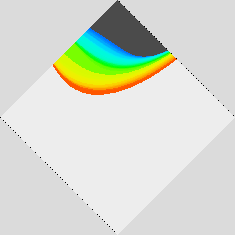
Figure 32: A rough plot of topological entropy throughout the unimodal region. Here the black area is the real shift locus with ${\bf h}=\log(2)$, the white area is the locus ${\bf h}=0$, and the colors represent intermediate values.

This has important consequences for topological entropy.

Remark (Filom’s work on Topological Entropy).

The topological entropy ${\bf h}(f)\geq 0$ is defined for much more general dynamical systems. For quadratic maps, it depends continuously on $f$, taking values in the interval $[0,\,\log(2)]$. For the relationship between entropy and kneading, see Remark 8 below.

Filom [F], showed that each locus of constant topological entropy is connected within the $~{}-+-~{}$ bimodal region, and also within the part of the unimodal region for which $f$ has an attracting periodic orbit. (This is the region above the curve ${\bf Per}_{1}(1)$ in Figure 17, or below the line ${\bf Per}_{1}(1)$ in Figure 20.) He conjectured that this is true throughout the unimodal region; and was able to prove this under the hypothesis that there are no bone-loops. Thus, using his work together with Section 8, we have the following.

Corollary .

Each locus of constant entropy in $\overline{\mathcal{U}}$ is connected.

For a different proof of this statement, see Yan Gao ([G]). His proof is based on the similar idea of showing that there is no bone-loop, but utilizes a completely different technique developed by Levin, Shen and van Strien in [LSS].

In the $~{}+-+~{}$ bimodal region Filom conjectured that the corresponding loci can be badly disconnected; and this was later proved by Filom and Pilgrim (see [FP]).

Remark (Entropy computed from Kneading).

In the unimodal case, the topological entropy ${\bf h}(f)$ is uniquely determined by the kneading invariant ${\bf K}_{1}(f)$; and hence is constant along each bone. In fact ${\bf h}(f)$ can easily be computed as a continuous monotone function of ${\bf K}_{1}(f)$: Simply note that a constant slope map, such as $F_{s}(x)=s|x|-1$ has topological entropy ${\bf h}(F_{s})=\log(s)$ for $1\leq s\leq 2$ (see [MS]). Since the correspondence $s\mapsto{\bf K}_{1}(F_{s})$ is strictly monotone and easily computable, it is not hard to locate the unique $s_{0}$ such that

$$\sup_{s<s_{0}}\,{\bf K}_{1}(F_{s})~{}\leq~{}{\bf K}_{1}(f)~{}\leq~{}\inf_{s>s_{0}}\,{\bf K}_{1}(F_{s})$$

to any required degree of accuracy; and it follows that the topological entropy is just ${\bf h}(f)=\log(s_{0})$. For a rough plot of entropy see Figure 32; which can be compared with Figure 30.)

The entropy $0\leq{\bf h}\leq\log(2)$ takes its maximal value of $\log(2)$ if and only if ${\bf K}_{1}=1$; and ${\bf h}=0$ if and only if ${\bf K}_{1}\leq~{}0.649816\ldots$.

Kneading theory is more complicated in the bimodal case, and computation of entropy from kneading theory is more difficult; but still quite feasible. (See Block and Keesling [BK].)

Appendix A The Simplest Examples.

This appendix will illustrate all possible combinatorics with $n\leq 4$, plus a few cases with $n=5$ and $n=6$, subject to a few restrictions. Specifically, we consider only those cases which are minimal and nonpolynomial (compare Section 2), and for which $\kappa\leq 0$. Cases with $\kappa>0$ can be obtained from these by orientation reversal (i.e., by a $180^{\circ}$ rotation of the graph.) Compare Section 3, together with Section 2.

This appendix is subdivided into two main sections: unobstructed and obstructed maps. Each section is divided into five parts: first the hyperbolic combinatorics of types B, C, and D, and then the half-hyperbolic and totally non-hyperbolic cases. The parameters $\mu$, $\kappa$, $\Sigma$ and $\Delta$ for all figures in the appendix are in Table LABEL:t-2.

menace

Unobstructed Combinatorics

Type B: Both critical points in a common periodic orbit.

   

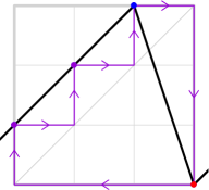
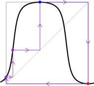
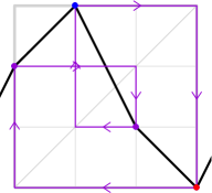
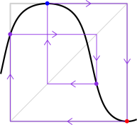
Figure 34: Co-polynomial maps of topological shape $+-$ . On the left are illustrations of a piecewise linear map and its corresponding rational map for the combinatorics ${(\!(}1,\,2,\,3,\,0{)\!)}$ with mapping pattern $\underline{\underline{x_{3}}}\mapsto x_{0}\mapsto x_{1}\mapsto\underline{\underline{x_{2}}}\mapsto\underline{\underline{x_{3}}}$ . On the right are illustrations for the combinatorics ${(\!(}2,\,3,\,1,\,0{)\!)}$ with mapping pattern $\underline{\underline{x_{3}}}\mapsto x_{0}\mapsto x_{2}\mapsto\underline{\underline{x_{1}}}\mapsto\underline{\underline{x_{3}}}$ .

   

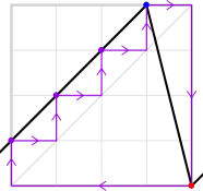
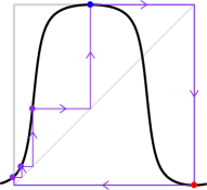
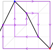
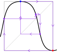
Figure 35: Co-polynomial maps of topological shape $+-$ . On the left are illustrations of a piecewise linear map and its corresponding rational map for the combinatorics ${(\!(}1,\,2,\,3,\,4,\,0{)\!)}$ with mapping pattern $\underline{\underline{x_{4}}}\mapsto x_{0}\mapsto x_{1}\mapsto x_{2}\mapsto\underline{\underline{x_{3}}}\mapsto\underline{\underline{x_{4}}}$. On the right are illustrations for the combinatorics ${(\!(}2,\,4,\,3,\,1,\,0{)\!)}$ with mapping pattern $\underline{\underline{x_{4}}}\mapsto x_{0}\mapsto x_{2}\mapsto x_{3}\mapsto\underline{\underline{x_{1}}}\mapsto\underline{\underline{x_{4}}}$ .

   

menace

Type C (Capture): One critical orbit lands in a cycle containing the other.

   

   

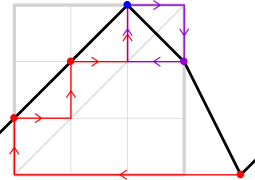
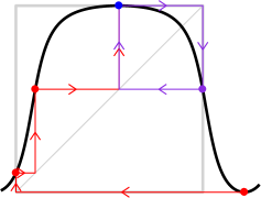
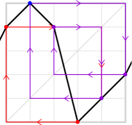
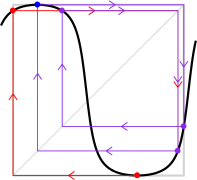
Figure 39: On the left are illustrations of a period two capture case of a strictly unimodal map of topological shape $+-$ , with combinatorics ${(\!(}1,\,2,\,3,\,2,\,0{)\!)}$ and with mapping pattern $\underline{\underline{x_{4}}}\mapsto x_{0}\mapsto x_{1}\mapsto\underline{\underline{x_{2}}}\leftrightarrow x_{3}$. As in the previous two cases, one critical point lies outside of $f({\widehat{\mathbb{R}}})$. On the right are illustrations of a capture component for $n=5$ with both critical points in $f(\widehat{{\mathbb{R}}})$, of topological shape $+-+$ , combinatorics ${(\!(}4,\,5,\,4,\,0,\,1,\,2{)\!)}$, and mapping pattern $\underline{\underline{x_{3}}}\mapsto x_{0}\mapsto x_{4}\mapsto\underline{\underline{x_{1}}}\mapsto x_{5}\mapsto x_{2}\mapsto x_{4}$ with a periodic critical orbit of period 4.

menace

Type D: Two disjoint critical orbits.

The only example of unobstructed combinatorics for $n\leq 6$ (up to orientation reversal) is the Wittner example (See figures 1 and 9). Furthermore, as a consequence of Section 7, there can be no unobstructed Type D examples with a period 2 orbit. An example of Type D with $n=8$ is shown in Figure 40.

  

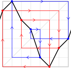
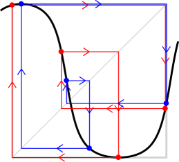
Figure 40: On the left, the PL model for the type D map of shape $+-+$ and combinatorics ${(\!(}6,\,7,\,5,\,4,\,1,\,0,\,2,\,3{)\!)}$, which has two period four critical orbits. The mapping pattern is $\underline{\underline{x_{1}}}\mapsto x_{7}\mapsto x_{3}\mapsto x_{4}\mapsto\underline{\underline{x_{1}}}$ and $\underline{\underline{x_{5}}}\mapsto x_{0}\mapsto x_{6}\mapsto x_{2}\mapsto\underline{\underline{x_{5}}}$. Its realization as a lifted map is shown on the right.

menace

Half-Hyperbolic: One critical orbit is periodic, the other is eventually repelling.

menace

Totally Non-Hyperbolic: Every postcritical cycle is repelling.

In these cases, since both critical orbits are eventually repelling, it follows that the complex Julia set is the entire Riemann sphere.

   

Figure 42: Maps of co-polynomial shape. On the left are illustrations of the piecewise linear map and its corresponding rational map for the combinatorics ${(\!(}2,\,3,\,2,\,0{)\!)}$ with dynamical pattern $\underline{\underline{x_{1}}}\mapsto\underline{\underline{x_{3}}}\mapsto x_{0}\mapsto x_{2}\,\rotatebox[origin={c}]{90.0}{\large$\circlearrowleft$}\,$. On the right are illustrations of the combinatorics ${(\!(}1,\,3,\,4,\,1,\,0{)\!)}$ with mapping pattern $\underline{\underline{x_{2}}}\mapsto\underline{\underline{x_{4}}}\mapsto x_{0}\mapsto x_{1}\leftrightarrow x_{3}$ .

   

Figure 43: On the left are illustrations of a map of co-polynomial shape with combinatorics ${(\!(}1,\,3,\,4,\,3,\,0{)\!)}$ and dynamical pattern $\underline{\underline{x_{2}}}\mapsto\underline{\underline{x_{4}}}\mapsto x_{0}\mapsto x_{1}\mapsto x_{3}\,\rotatebox[origin={c}]{90.0}{\large$\circlearrowleft$}\,$ . On the right are illustrations of a map of topological shape $+-+$, with combinatorics ${(\!(}3,\,4,\,6,\,3,\,1,\,0,\,1{)\!)}$. The mapping pattern is $\underline{\underline{x_{2}}}\mapsto x_{6}\mapsto x_{1}\leftrightarrow x_{4}$ and $\underline{\underline{x_{5}}}\mapsto x_{0}\mapsto x_{3}\,\rotatebox[origin={c}]{90.0}{\large$\circlearrowleft$}\,$

.

menace

Strongly Obstructed Combinatorics

Since for strongly obstructed combinatorics the limit cannot be realized as a rational map, the images of limiting maps will use the convention of Figure 11 in Section 4, indicating the marked points by disks and their images under the map by open squares. In some cases, the square will appear to be filled, because the image is another marked point.

Type B: Both critical points in a common periodic orbit.

For Type B, strongly obstructed examples seem to be uncommon. The smallest example we were able to find has $n=6$.

  

menace

Type C: One critical orbit lands in a cycle containing the other.

 

menace

Type D: Disjoint periodic critical orbits.

Unlike the Type B case, strongly obstructed dynamics of Type D are common.

 

 

 

menace

Half-Hyperbolic: One critical orbit is periodic, but the other is eventually repelling.

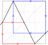
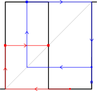
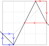
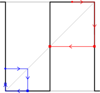
Figure 49: On the left, a strongly obstructed case of topological shape $+-+$ with combinatorics ${(\!(}2,\,4,\,2,\,0,\,1{)\!)}$.The mapping pattern is $\underline{\underline{x_{1}}}\leftrightarrow x_{4}$; and $\underline{\underline{x_{3}}}\mapsto x_{0}\mapsto x_{2}\,\rotatebox[origin={c}]{90.0}{\large$\circlearrowleft$}\,$. On the right, combinatorics ${(\!(}1,\,0,\,2,\,4,\,2{)\!)}$, topological shape $-+-$, and mapping pattern $\underline{\underline{x_{1}}}\leftrightarrow x_{0}$ and $\underline{\underline{x_{3}}}\mapsto x_{4}\mapsto x_{2}\,\rotatebox[origin={c}]{90.0}{\large$\circlearrowleft$}\,$. This is the “left-right reflected” version of the picture on the left.

Totally Non-Hyperbolic: Every postcritical cycle is repelling.

  

Appendix B Further Information about the Figures

After a preliminary remark, this appendix will consist of a brief Table B.1 which classifies figures according to their dynamic type and topological shape, and the more extensive LABEL:t-2 which lists their combinatorics and parameters.

Remark (Constraints on the parameters).

Note that:

$$\textrm{Shape}~{}~{}+-+~{}~{}\textrm{or~{} co-polynomial} \Longrightarrow \quad\Sigma\,\in\,[-1,\,0]~{},$$

$$\textrm{Shape}~{}~{}-+-~{}~{}\textrm{or~{} polynomial} \Longrightarrow \quad\Sigma\,\in\,[0,\,1]~{}.$$

On the other hand,

$$\textrm{for the}~{}~{}-+~{}~{}\textrm{combinatorics,} \Sigma \in\;[-0.5,\,0.5]\,$$

$$\textrm{while for}~{}~{}+-~{}~{}\textrm{combinatorics,} \Sigma \in\;[-1,\,-0.5]\,\cup\,[0.5,\,1]~{}.$$

(Compare Figure 15.) Note that $\mu$ and $\Delta$ are invariant under orientation reversal. However, $\kappa$ changes sign and $\Sigma$ is replaced by $\pm 1-\Sigma~{}$.

Recall that all combinatorics of topological shape $-+-$ are obstructed; but that combinatorics of unimodal shape are unobstructed, except possibly in the totally non-hyperbolic case. (Compare Section 2, as well as Section 3 and Section 8.)

Table B.1: A list of figure numbers classified according to their dynamic type and topological shape. It includes figures which illustrate minimal and non-polynomial combinatorics, We provide at least one example for each combination which can actually occur, with the possible exception of the totally non hyperbolic unimodal case where we conjecture that there are no examples. Note that Figures 12, 33L, and 42L are the only examples with Euclidean orbifold; and that Figure 12 is the only example where the rational function exists but the Thurston algorithm usually doesn’t converge (compare Figure 13).

Unobstructed
	B	C	D	Half	Totally Non-
				Hyperbolic	Hyperbolic
co-poly	33LR, 34LR,	none	none	none	42LR, 43L
	35LR, 36L
$+-+$	36R, 37	39R	1, 40	41R	43R
unimodal	none	2, 10, 38LR, 39L	none	41L	12
Obstructed
$+-+$	44	45L	46L, 47L, 48LR	49L	50
$-+-$	none	45R	46R, 47R	49R	51LR
unimodal	none	none	none	none	none ?

Table B.2: This table lists the parameters for all of the figures which illustrate some combinatorics. Parameters for the “corresponding polynomials” of Table 8.0 are also listed. Here $N$ denotes the number of iterations that were used in producing the figures, starting with the points of ${\stackrel{{\scriptstyle\rightarrow}}{{x}}}$ equally spaced within the appropriate intervals and continuing until $(\Sigma,\Delta)$ was within $10^{-7}$ of the limiting value. However, two examples require special mention: The $*$ in the “N” column for Figure 12 indicates that the data for this exceptional case had to be computed directly, without any iteration. The entries for Figure 13 show what actually happens when we iterate with this combinatorics. (In fact the initial conditions for Figure 13 were specially chosen, but any generic choice would yield similar behavior.) In the unobstructed cases the parameters $\mu$ and $\kappa$ (or $\Sigma$ and $\Delta$) of the limit map uniquely determine the combinatorics; but this is not true for strongly obstructed cases (characterized by $\mu=\pm\infty$ or by $\Delta=1$). The converse statement that the combinatorics determines the parameters is true in all cases. The parameter $\Sigma\in{\mathbb{R}}/2{\mathbb{Z}}$ is always specified by its representative in the interval $(-1,\,1]$.

figure	combinatorics	$N$	$\mu$	$\kappa$	$\Sigma$	$\Delta$
1, 9	${(\!(}5,6,4,1,0,2,3{)\!)}$	87	$-7.2407034$	$\phantom{-}1.097305$	$-0.338652$	$0.836756$
2	${(\!(}1,2,3,2,0{)\!)}$	63	$-1.270048$	$-1.351520$	$\phantom{-}0.893946$	$0.561904$
5	$\stackrel{{\scriptstyle\hbox{${(\!(}4,2,1,0,1{)\!)}$}\rule{0.0pt}{9.64441pt}\rule[-3.61664pt]{0.0pt}{0.0pt}}}{{\hbox{${(\!(}3,1,0,1{)\!)}$}}}$	$\stackrel{{\scriptstyle\hbox{$12$}\rule[-3.61664pt]{0.0pt}{0.0pt}}}{{\hbox{$\phantom{1}2$}}}$	$-4$	$\phantom{-}1$	-0.271699	0.728301
6	${(\!(}3,5,3,2,0,2{)\!)}$	6	$-\infty$	$\phantom{-}0$	$-1/2$	$1$
10	${(\!(}3,2,1,2{)\!)}$	43	$-1.295581$	$\phantom{-}1.191483$	$\phantom{-}0$	$1/2$
11	${(\!(}1,2,4,5,2,1,0{)\!)}$	42	$-2.594313$	$-1.637869$	$\phantom{-}1$	$0.712071$
12	${(\!(}1,3,4,3,1,0{)\!)}$	*	$-2$	$-\sqrt{2}$	$\phantom{-}1$	$0.635940$
		odd	$-8/3$	$-5/3$	$\phantom{-}1$	$0.719622$
13	${(\!(}1,3,4,3,1,0{)\!)}$	even	$-3/2$	$-5/4$	$\phantom{-}1$	$0.545629$
21L	${(\!(}3,5,3,2,1,0{)\!)}$	14	$-4$	$-1$	$-0.728301$	$0.728301$
21R	${(\!(}3,4,3,2,1,0{)\!)}$	48	$-4/3$	$-1$	$-0.892232$	$0.455511$
22	${(\!(}2,0,1,2,5,3{)\!)}$	9	$\phantom{-}\infty$	$-1$	$1/2$	$1$
25	${\rm FP}(8,9)$	$1000$	$-256.3050$	$-1.494245$	$-0.507393$	$0.995033$
28L	${(\!(}3,2,0,1{)\!)}$	14	$-3.796781$	$\phantom{-}0.898403$	$-0.287930$	$0.712070$
28LC	${(\!(}3,2,0,1,4{)\!)}$	31	$\phantom{-}3.498562$	$\phantom{-}0.749281$	$\phantom{-}0.258130$	$0.741869$
29L	${(\!(}4,3,0,1,3{)\!)}$	23	$-5.538584$	$\phantom{-}1.769292$	$-0.182973$	$0.817027$
29LC	${(\!(}4,3,0,1,3,5{)\!)}$	24	$\phantom{-}3.890875$	$\phantom{-}0.945437$	$\phantom{-}0.223012$	$0.776988$
33L	${(\!(}1,0{)\!)}$	1	$-2$	$\phantom{-}0$	$-1/2$	$\phantom{-}1/2$
$\stackrel{{\scriptstyle\hbox{corresp.}}}{{\hbox{poly}}}$	${(\!(}0,2,1{)\!)}$	12	$\phantom{-}3.236068$	$-0.618034$	$\phantom{-}0.712071$	$0.712071$
4, 33R	${(\!(}1,2,0{)\!)}$	12	$-4.649436$	$-1.324718$	$-0.772304$	$0.772304$
$\stackrel{{\scriptstyle\hbox{corresp.}}}{{\hbox{poly}}}$	${(\!(}0,2,3,1{)\!)}$	12	$\phantom{-}3.831874$	$-0.915937$	$\phantom{-}0.772304$	$0.772304$
34L	${(\!(}1,2,3,0{)\!)}$	69	$-5.968584$	$-1.984292$	$-0.833802$	$0.833802$
$\stackrel{{\scriptstyle\hbox{corresp.}}}{{\hbox{poly}}}$	${(\!(}0,2,3,4,1{)\!)}$	12	$\phantom{-}3.960270$	$-0.9801349$	$\phantom{-}0.782264$	$0.782264$
34R	${(\!(}2,3,1,0{)\!)}$	12	$-3.796780$	$-0.898402$	$-0.712071$	$0.712071$
$\stackrel{{\scriptstyle\hbox{corresp.}}}{{\hbox{poly}}}$	${(\!(}0,3,4,2,1{)\!)}$	31	$\phantom{-}3.498562$	$-0.749281$	$\phantom{-}0.741869$	$0.741869$
35L	${(\!(}1,2,3,4,0{)\!)}$	90	$-6.656438$	$-2.328219$	$-0.855761$	$0.855761$
$\stackrel{{\scriptstyle\hbox{corresp.}}}{{\hbox{poly}}}$	${(\!(}0,2,3,4,5,1{)\!)}$	13	$\phantom{-}3.990267$	$-0.995134$	$\phantom{-}0.784470$	$0.784470$
35R	${(\!(}2,4,3,1,0{)\!)}$	13	$-4.044724$	$-1.022362$	$-0.731704$	$0.731704$
$\stackrel{{\scriptstyle\hbox{corresp.}}}{{\hbox{poly}}}$	${(\!(}0,3,5,4,2,1{)\!)}$	24	$\phantom{-}3.738915$	$-0.869457$	$\phantom{-}0.764527$	$0.764527$
36L	${(\!(}1,3,4,2,0{)\!)}$	44	$-5.628255$	$-1.814128$	$-0.820750$	$0.820750$
$\stackrel{{\scriptstyle\hbox{corresp.}}}{{\hbox{poly}}}$	${(\!(}0,2,4,5,3,1{)\!)}$	12	$\phantom{-}3.905709$	$-0.952855$	$\phantom{-}0.778136$	$0.778136$
36R	${(\!(}2,3,4,0,1{)\!)}$	88	$-18.46037$	$-1.433732$	$-0.592613$	$0.932596$
37	${(\!(}2,3,4,5,6,0,1{)\!)}$	100	$-25.104560$	$-3.261693$	$-0.655923$	$0.952150$
38L	${(\!(}1,2,1,0{)\!)}$	61	$-1.295598$	$-1.191488$	$1$	$\phantom{-}1/2$
38R	${(\!(}1,2,3,1,0{)\!)}$	62	$-2.340346$	$-1.539254$	$1$	$0.682963$
39L	${(\!(}1,2,3,2,0{)\!)}$	63	$-1.270048$	$-1.351520$	$\phantom{-}0.893945$	$0.561904$
39R	${(\!(}4,5,4,0,1,2{)\!)}$	25	$-8.401378$	$\phantom{-}0.770864$	$-0.399338$	$0.854152$
40	${(\!(}6,7,5,4,1,0,2,3{)\!)}$	38	$-5.333358$	$\phantom{-}0.972001$	$-0.318689$	$0.784399$
41L	${(\!(}2,3,2,1,0{)\!)}$	22	$-1.333333$	$-1$	$-0.8929233$	$0.455512$
41R	${(\!(}3,4,6,5,4,0,1{)\!)}$	68	$-6.704389$	$-1.109249$	$-0.673413$	$0.825583$
42L	${(\!(}2,3,2,0{)\!)}$	2	$-4$	$-1$	$-0.728301$	$0.728301$
$\stackrel{{\scriptstyle\hbox{corresp.}}}{{\hbox{poly}}}$	${(\!(}0,3,4,3,1{)\!)}$	40	$\phantom{-}3.678573$	$-0.839287$	$\phantom{-}0.759201$	$0.759201$
42R	${(\!(}1,3,4,1,0{)\!)}$	23	$-5.538584$	$-1.769292$	$-0.817021$	$0.817021$
$\stackrel{{\scriptstyle\hbox{corresp.}}}{{\hbox{poly}}}$	${(\!(}0,2,4,5,2,1{)\!)}$	24	$\phantom{-}3.890873$	$-0.945436$	$\phantom{-}0.776988$	$0.776988$
43L	${(\!(}1,3,4,3,0{)\!)}$	53	$-5.678573$	$-1.839286$	$-0.822747$	$0.822747$
$\stackrel{{\scriptstyle\hbox{corresp.}}}{{\hbox{poly}}}$	${(\!(}0,2,4,5,4,1{)\!)}$	15	$\phantom{-}3.927737$	$-0.963869$	$\phantom{-}0.779808$	$0.779808$
43R	${(\!(}3,4,6,3,1,0,1{)\!)}$	99	$-8.266304$	$-1$	$-0.632072$	$0.853973$
44	${(\!(}3,5,4,1,0,2{)\!)}$	6	$-\infty$	$\phantom{-}0$	$-1/2$	$1$
45L	${(\!(}2,4,1,0,1{)\!)}$	13	$-\infty$	$-1$	$-1/2$	$1$
45R	${(\!(}1,0,1,4,2{)\!)}$	13	$\phantom{-}\infty$	$-1$	$\phantom{-}1/2$	$1$
46L	${(\!(}2,3,0,1{)\!)}$	22	$-\infty$	$\phantom{-}0$	$-1/2$	$1$
7, 46R	${(\!(}1,0,3,2{)\!)}$	22	$\phantom{-}\infty$	$\phantom{-}0$	$\phantom{-}1/2$	$1$
47L	${(\!(}2,4,3,0,1{)\!)}$	12	$-\infty$	$-1$	$-1/2$	$1$
47R	${(\!(}1,0,3,4,2{)\!)}$	13	$\phantom{-}\infty$	$-1$	$\phantom{-}1/2$	$1$
48L	${(\!(}3,4,5,1,0,2{)\!)}$	40	$\phantom{-}\infty$	$-0.618034$	$-1/2$	$1$
48R	${(\!(}4,5,0,1,2,3{)\!)}$	69	$-\infty$	$\phantom{-}\infty$	$-1/2$	$1$
49L	${(\!(}2,4,2,0,1{)\!)}$	13	$-\infty$	$-1$	$-1/2$	$1$
49R	${(\!(}1,0,2,4,2{)\!)}$	13	$\phantom{-}\infty$	$-1$	$\phantom{-}1/2$	$1$
50	${(\!(}3,5,4,3,0,2{)\!)}$	5	$-\infty$	$-1$	$-1/2$	$1$
51L	${(\!(}2,0,3,5,6,5,3{)\!)}$	8	$\phantom{-}\infty$	$\phantom{-}1$	$\phantom{-}1/2$	$1$
51R	${(\!(}2,0,4,5,6,5,3{)\!)}$	9	$\phantom{-}\infty$	$\phantom{-}1$	$\phantom{-}1/2$	$1$

Table B.2: Continued from previous page

Araceli Bonifant: Mathematics Department, University of Rhode Island, Kingston, R.I., 02881. email: bonifant@uri.edu

John Milnor: Institute for Mathematical Sciences, Stony Brook University, Stony Brook, NY. 11794-3660. email: jack@math.stonybrook.edu

Scott Sutherland: Institute for Mathematical Sciences, Stony Brook University, Stony Brook, NY. 11794-3660. email: scott@math.stonybrook.edu

References

- [BK] L. Block, J. Keesling, Computing the topological entropy of maps of the interval with three monotone pieces, J. Stat. Phys. 66 (1992) 755–774. doi:10.1007/BF01055699
- [BMS] A. Bonifant, J, Milnor and S. Sutherland, The W. Thurston algorithm applied to real polynomial maps, arXiv:2005.07800 [] (2020).
- [BS] H. Bruin and D. Schleicher, Admissibility of kneading sequences and structure of Hubbard trees for quadratic polynomials, Journal of the London Math. Soc. 78 (2008) 502–522. doi:10.1112/jlm
- [DGMT] S. Dawson. R. Galeeva, J. Milnor, and Ch. Tresser, A monotonicity conjecture for real cubic maps, In Real and Complex Dynamical Systems (Hillerød, 1993), 464 of NATO Adv. Sci. Inst. Ser. C Math. Phys. Sci., pages 165–183. Kluwer Acad. Publ., Dordrecht, (1995).
- [DH] A. Douady and J. H. Hubbard, A proof of Thurston’s topological characterization of rational functions, Acta Math. 171 2 (1993) 263–297. doi:10.1007/BF02392534.
- [D] L. DeMarco, The moduli space of quadratic rational maps. Journal of the AMS. 20 (2007) 321–355. doi:10.1090/S0894-0347-06-00527-3
- [E] A. Epstein, Bounded hyperbolic components of quadratic rational maps. Ergodic Theory Dynam. Systems 20 (2000) 727–748. doi:10.1017/S0143385700000390
- [F] K. Filom, Monotonicity of entropy for real quadratic rational maps. arXiv:1901.03458 [math.DS] (2019)
- [FP] K. Filom and K. Pilgrim, On the non-monotonicity of entropy for a class of real quadratic rational maps. Journal of Modern Dynamics, 16 (2020) 225–254. doi:10.3934/jmd.2020008
- [G] Y. Gao, Monotonicity of entropy for unimodal real quadratic rational maps arXiv:2009.03797 [math.DS] (2020)
- [KL] G. Kelsey and R. Lodge, Quadratic Thurston maps with few postcritical points, Geom. Dedicata, 201 (2019) 33–55. doi:10.1007/s10711-018-0387-5
- [KR] J. Kiwi and M. Rees, Counting hyperbolic components, J. Lond. Math. Soc. 88 (2013) 669–698. doi:10.1112/jlms/jdt027
- [LSS] G. Levin, W. Shen and S. van Strien, Positive Transversality via transfer operators and holomorphic motions with applications to monotonicity for interval maps, arXiv:1902.06732 [math.DS], doi:10.1088/1361-6544/ab853e
- [M] J. Milnor, Geometry and dynamics of quadratic rational maps. Experiment. Math. 2 (1993) 37–83. doi:10.1080/10586458.1993.10504267
- [MS] M. Misiurewicz and W. Szlenk, Entropy of piecewise monotone mappings. Astérisque 50 (1977) 299–310; or Studia Math. 67 (1980) 45–63. doi:10.4064/sm-67-1-45-63.
- [MTh] J. Milnor and W. Thurston, On iterated maps of the interval. Dynamical Systems (College Park, MD, 1986–87), 465–563, Lecture Notes in Math. 1342 Springer, Berlin (1988). doi:10.1007/BFb0082847
- [MTr] J. Milnor and Ch. Tresser, On entropy and monotonicity for real cubic maps with an appendix by A. Douady and P. Sentenac. Comm. Math. Phys. 209 (2000) 123–178. doi:10.1007/s002200050018
- [P] A. Poirier, Hubbard trees. Fund. Math. 208 (2010) 193–248. doi:10.4064/fm208-3-1.
- [R] M. Rees, Components of degree two hyperbolic rational maps. Invent. Math. 100 (1990) 357–382. doi:10.1007/BF01231191
- [S] N. Selinger, Thurston’s pullback map on the augmented Teichmüller space and applications. Invent. Math. 189 (2012) 111–142. doi:10.1007/s00222-011-0362-3.
- [T] Tan Lei, Matings of quadratic polynomials, Ergodic Theory Dyn. Sys. 2 (1992) 589–620. doi:10.1017/S0143385700006957
- [W] B. Wittner, On the bifurcation loci of rational maps of degree two. Thesis, Cornell University, 1988. http://math.stonybrook.edu/theses/thesis86-1/part1.pdf