Extreme compression of grayscale images

Abstract.

Given an grayscale digital image, and a positive integer $n$, how well can we store the image at a compression ratio of $n:1$?

In this paper we address the above question in extreme cases when $n>>50$ using “$\mathbf{V}$-variable image compression”.

1. Introduction

A digital $j\times k$ pixels image consists of $j\cdot k$ pixels where each pixel is assigned a “colour”, i.e. an element of some finite set, $C$, e.g. $C=\{0,1,2,\ldots,255\}^{l}$, where $l=1$ for (8 bit) grayscale images or $l=3$ for (24 bit RGB) colour images.
Image compression methods can be of two types: Lossless image compression methods preserves all image data, while lossy methods removes some data from the original file and saves an approximate image with reduced file size.

One common lossless format on the internet, supported by most modern web-browsers, is PNG (Portable Network Graphics). The PNG format is used in particular for images with sharp colour contrast like text and line art, and is considered to be a suitable format for storing images to be edited.

One disadvantage with lossless formats is that the file sizes are often very large when compared with lossy formats. Lossy compression of colour images is often obtained by reducing the colour space, or by chroma subsampling using the fact that the human eye perceives changes in brightness more sharply than changes in colour.

The most common lossy compression format, especially for photographic images, is JPEG (Joint Photographic Experts Group). JPEG usually gives small file sizes, but one artifact with JPEG is apparent “halos” in parts of the image with sharp colour contrasts, reflecting the fact that the JPEG method belongs to the realm of Fourier methods. Similar “halo” features are also apparent in the better, but more complicated and therefore less widespread, wavelet based JPEG 2000 method.

The mathematical notion of $V$-variability was introduced by Barnsley, Hutchinson and Stenflo in [2]. Intuitively, a $V$-variable set is built up by at most $V$ different smaller sets at any given level of magnification. Motivated by the fact that parts of an image often resemble other parts of the image, and the existing “fractal compression method” building on a more limited class of sets [1], it was suggested in [2] that $V$-variability could be used for image compression.

One solution to the problem of how the notion of $V$-variability can be used for image compression was presented in Mendivil and Stenflo [3] in terms of an algorithm for lossy image compression where, for a given digital image, the algorithm generates a “$V$-variable digital image” resembling the given image despite requiring substantially less storage space.

In the present paper we address the question of finding an “optimal” $V$-variable digital image resembling a target image given a certain maximally allowed storage space.

2. $\mathbf{V}$-variable image compression

For clarity and simplicity of our description we will assume here that the image is of size $2^{m}\times 2^{m}$ pixels for some $m$. We refer to Section 4.1 for the case of non-square images.

In order to specify what we mean by a “$V$-variable digital image” (and later a “$\mathbf{V}$-variable digital image”) we need to introduce some definitions.

Definition 1.

Let $m\geq 0$ be some integer, and consider a $2^{m}\times 2^{m}$ pixels digital image. For any $0\leq n\leq m$, we may divide the given image into $4^{n}$ nonoverlapping image pieces of size $2^{m-n}\times 2^{m-n}$. We call these pieces the image pieces of level $n$.

We can now define what we mean by a $V$-variable image:

Definition 2.

Let $V\geq 1$ be a fixed positive integer. We say that a digital image is $V$-variable if, for any $1\leq n\leq m$, the image has at most $V$ distinct image pieces of level $n$.

Example 1.

The $4$-variable $512\times 512=2^{9}\times 2^{9}$ pixels digital grayscale image

can be built up by $4^{n}$ image pieces of size $2^{9-n}\times 2^{9-n}$ of (at most) $4$ distinct types, for any $n=0,1,2,\ldots,9$. The appearance of these image pieces depends on $n$. If e.g.  $n=2$ then the $16$ image pieces of size $128\times 128$ pixels are of the $4$ types

and if $n=3$ then the $64$ image pieces of size $64\times 64$ pixels are of the $4$ types

By looking at the image, and its image pieces, we see that we can, recursively, describe the $4$-variable image using $4$ images of smaller and smaller size, i.e. recursively describe more and more levels of the $V$-variable structure of the image:

At each stage, we replace an image piece of the current level with four image pieces from the next level. There are (at most) $V=4$ types of image pieces at each level and the substitution is done according to the type. For example, we see that in the second stage (illustrated in the figure above), all image pieces of type $3$ are replaced by the same thing (image pieces at next level with types $3,4,3,4$). The first two (non-trivial) steps as shown above can be visually described by the substitutions:

Each image piece of level 9 is a one pixel image. For such pieces we associate the corresponding colour value.

In this $4$-variable example the image is constructed using only the $4$ colour values $33$ and $37$ (corresponding to the almost black pixels) $138$ (corresponding to the dark gray pixels) and $171$ (corresponding to the light gray pixels).

See [3] and Section 2.3 for further details and the specifics on how to reconstruct the image from its code (the substitution rules).

2.1. Description of our $V$-variable image compression method

The goal of our method is to approximate a given digital image with a $V$-variable digital image.

We start with positive integers $V_{1},V_{2},\ldots,V_{m}$ which restrict the number of distinct image pieces, of each level $n$, $n=1,2,\ldots,m$. Note that by our choice of partitions at each of the “levels”, there are at most four times as many distinct image pieces of level $n+1$ as there were at level $n$. Thus any value of $V_{n}$ which is at least $\min(4^{n},4V_{n-1})$ provides no constraint that is not already forced by $V_{1},\ldots,V_{n-1}$.

Let $V=\max(V_{1},\ldots,V_{m})$. We can find a $V$-variable approximation of the given image, with $V_{1}$,…,$V_{m}$ being restrictions on the maximum number of allowed distinct image pieces of each level respectively, by using the following algorithm:

In [3], we formulated and applied the above algorithm for various choices of $V$ and images, where $m=9$ and $V=V_{1}=\ldots=V_{m}$ (and so we only considered images which had the same “maximal variability” at each level).

The above algorithm with non-constant $V_{n}$ generates a $V$-variable image for $V=\max(V_{1},\ldots,V_{m})$ with less memory requirements than the $V=V_{1}=\ldots=V_{m}$ case considered in [3], but the image quality is also decreased. The art is then to try to find the optimal $m$-tuple of positive integers ${\mathbf{V}}=(V_{1},\ldots,V_{m})$ with respect to targeted image quality and memory requirements.

We will present computer experiments related to this question for some given test images below.

See Section 4 for a discussion of some generalizations of the algorithm.

Definition 3.

Let ${\mathbf{V}}=(V_{1},\ldots,V_{m})$, and $V=\max(V_{1},\ldots,V_{m})$, where $V_{1},\ldots,V_{m}$ is a given sequence of positive integers. We say that an $2^{m}\times 2^{m}$ pixels digital image is $\mathbf{V}$-variable if it is $V$-variable with maximally $V_{i}$ distinct image pieces of level $i$, for any $i=1,\ldots,m$.

2.2. Storage requirements

The $m$-tuple of positive integers ${\mathbf{V}}=(V_{1},\ldots,V_{m})$ , chosen by the user in step 1 in the algorithm above, corresponds to the quality of the image approximation. Larger values of the components corresponds to higher image quality of the constructed V-variable image at the price of a larger file size. We may without loss of generality assume that $V_{i}\leq\min(4^{i},4V_{i-1})$ for all $1\leq i\leq m$ (with the convention $V_{0}=1$):

Each execution of step $4$ requires a storing of $4V_{j-1}$ numbers from the range $\{1,\ldots,V_{j}\}$ for any $j$, $n_{0}\leq j\leq m-1$. The image pieces extracted in step $2$ are of size $4^{m-n_{0}}$ pixels, and each time step $5$ is reached the new image pieces are $4$ times smaller than the ones from the previous execution of step 5. Thus step $4$ will be revisited at most $m-n_{0}-1$ times.

In step $6$ we store the colour, i.e.  an element in $C$, for each of the $4V_{m-1}$ “one pixel” image representatives. As an example, for the 8 bit grayscale images considered in this paper we need to store $4V_{m-1}$ numbers in $\{0,\ldots,255\}$, and we may thus, in order to optimize the image quality for a given storage space, without loss of generality assume that $V_{m}=256$ since the storage does not depend on $V_{m}$.

Thus, our $V$-variable method of storing requires in total $4V_{j-1}\lceil{\log_{2}(V_{j}}\rceil/8$ bytes for each level $n_{0}\leq j\leq m-1$, where $4V_{j-1}>V_{j}$, plus $4V_{m-1}$ bytes for level $m$ in the 8 bit grayscale images case.

Remark 1.

We will here only consider the case when $m=9$ and $4V_{k}\geq V_{k+1}$ for all $k$. In order to avoid a waste of memory we will also only consider cases when $V_{k}=2^{j_{k}}$ for some $j_{k}$ for all $k$, where $V_{n_{0}-1}=4^{n_{0}-1}$ giving a total storage (in the case $m=9$) of

$$\text{Storage}=\sum_{k\in I}4V_{k-1}\lceil{\log_{2}(V_{k}}\rceil/8+4V_{8}=\sum_{k\in I}j_{k}2^{j_{k-1}-1}+2^{j_{8}+2}\ \ \ \text{ bytes},$$

where $I=\{n_{0}\leq k\leq 8:V_{k}<4V_{k-1}\}$. Each $k$ with $V_{k}=4V_{k-1}$ gives no contribution to the sum so for instance if $V_{4}=4^{4}=256$, $V_{5}=2^{8}=256<4^{5}$, $V_{6}=2^{5}=32$, $V_{7}=4V_{6}=128$, $V_{8}=2^{6}=64$ then $n_{0}=5$, $j_{4}=8$, $j_{5}=8$, $j_{6}=5$, $j_{7}=7$, and $j_{8}=6$ and thus

$$\text{Storage}=8\cdot\underbrace{2^{8-1}}_{128}+5\cdot\underbrace{2^{8-1}}_{128}+0+6\cdot\underbrace{2^{7-1}}_{64}+\underbrace{2^{6+2}}_{256}=2304\ \ \ \text{ bytes},$$

where the zero term occur since $4V_{6}=V_{7}$, and thus $V_{7}$ causes no new restrictions not already caused by $V_{1}$,…,$V_{6}$.

2.3. Reconstruction of an image from its code

The process of reconstructing an image from its $V$-variable code is quick.

Any pixel sits within some fixed image piece of level $n$ for all $0\leq n\leq m-1$. An image piece of level $n$, $1\leq n\leq m$, is situated within a 4 times bigger image piece from level $n-1$ and can be in 4 possible positions in that bigger square:
  1) upper left, or  2) upper right, or  3) lower left, or  4) lower right.
This enables a simple addressing structure, where a pixel can be described by an address $a_{1}a_{2}...a_{m}$, where $a_{j}\in\{1,2,3,4\}$ specifies the relative position of the square on level $j$ in the square on level $j-1$ for the given pixel.

We can now find the colour of a pixel by recursively using the $V$-variable code in the following way. If a pixel with address $a_{1}a_{2}...a_{m}$ sits within a square with $V$-variable type $j$ of level $n$, $0\leq n\leq m-1$, then the $V$-variable type of the square on level $n+1$ where the pixel sits can be seen by looking at the stored type of the square in position $a_{n+1}$ within the square of type $j$ on level $n$. The colour of the pixel is given by the stored colour of the square in position $a_{m}$ of the type of the square at level $m-1$.

2.4. Automating the $V$-variable image compression algorithm

The main tool needed in order to automate the algorithm above is a way to classify $n$ images into $k$ clusters. (step 3). Such a clustering can be done in many different ways. See Section 4.2 for a discussion of some basic clustering techniques. For simplicity, in our implementation of the compression algorithm above we used Matlab’s built-in command kmeans for this step. The K-means algorithm is a popular and basic clustering algorithm which finds clusters and cluster representatives for a set of vectors by iteratively minimising the sum of the squares of the “within cluster” distances (the distances from each of the vectors to the closest cluster representative). We treat the sub-images as vectors and use the standard Euclidean distance to measure similarity. We also use random initialisation of the cluster representatives.

2.5. Finding the optimal $\mathbf{V}$ for a given memory requirement

For a given image and tuple $\mathbf{V}=(V_{1},\ldots,V_{m})$ we may use the algorithm described in Section 2.1 to generate a $\mathbf{V}$-variable approximating image of the given image and in Section 2.2 we explained how to calculate an upper bound for the memory requirement for a $\mathbf{V}$-variable image.

A natural problem that arises is to find the optimal $\mathbf{V}$ for a given memory requirement with respect to image quality. The optimal choice may depend on the image, but in general simulations show that a “good” $\mathbf{V}$ is often “good” for most images.

Rather than finding the optimal choice for a a given image and memory requirement we will here give rules of thumb for choices of $\mathbf{V}$ for some given memory requirements that may be used for any image.

2.6. Simulations

In this section we present results of some numerical experiments with the three images shown in Figure 1. The images are of size $512\times 512$ pixels so uncompressed they are stored with $512\cdot 512=262144$ B (since each pixel is assigned a number in $\{0,1,\ldots,255\}$ and thus requires one byte of storage). Thus approximations stored e.g. with a file size of 2621 B correspond to a 100:1 compression ratio. As can be seen, the three images represent a wide range of image types.

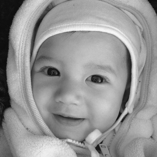
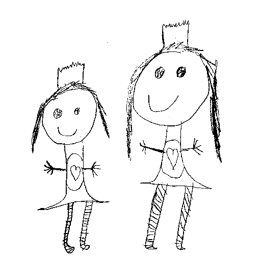
Figure 1. Three test images: Image1, Image2, Image3

Image1 and Image2 have earlier been discussed in [3].

We will here use the Peak signal-to-noise ratio (PSNR) for measuring quality of compressed images. Figure 2 shows the quality of $\mathbf{V}$-variable approximations of Image1 (PSNR) versus memory requirement for all $\mathbf{V}=(V_{1},\ldots,V_{9})$ requiring a memory less than 5000 B with $V_{1}=4,V_{2}=16,V_{3}=64$ and $V_{9}=256$ and $V_{4},V_{5},V_{6},V_{7}$ and $V_{8}$ chosen from $\{16,32,64,128,256,1024\}$.

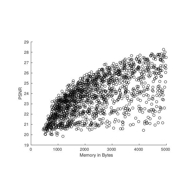
Figure 2. Scatterplot of filesize versus PSNR for Image1

The frontier in the plot gives a hint of how the optimal PSNR depends on the memory requirement.

The table in Figure 3 gives rules of thumb for good tuples $\mathbf{V}$ for given memory requirements of $1000\mathrm{B},1500\mathrm{B},\ldots,5000\mathrm{B}$ respectively. These $\mathbf{V}$:s corresponds to points close to the frontier in Figure 2. In simulations below “ImageI-Memory” denotes the $\mathbf{V}$-variable image obtained from the algorithm to approximate ImageI, I $\in\{1,2,3\}$, with a maximal allowed memory of Memory $\in\{500,1000,\ldots,5000\}$ Bytes using the rules of thumb for $\mathbf{V}=(V_{1},\ldots,V_{9})$ given by Figure 3.

The image labeled ImageI:256 correspond to the best $256$-variable approximation w.r.t. PSNR and has earlier been discussed in [3].

Label	$V_{4}$	$V_{5}$	$V_{6}$	$V_{7}$	$V_{8}$	Memory (B)	PSNR Image1	PSNR Image2	PSNR Image3
ImageI-500	16	16	16	16	64	480	20.6	15.1	13.9
ImageI-1000	256	32	16	16	64	992	23.5	15.9	14.7
ImageI-1500	256	64	64	32	64	1472	24.5	16.3	15.3
ImageI-2000	128	512	32	32	64	1936	25.4	16.9	16.5
ImageI-2500	256	256	32	128	64	2304	25.9	17.1	16.8
ImageI-3000	256	256	64	128	128	2976	26.5	17.4	17.2
ImageI-3500	256	256	1024	16	64	3328	26.8	17.9	18.4
ImageI-4000	256	1024	64	128	64	3936	27.5	18.6	17.3
ImageI-4500	256	256	1024	64	64	4544	27.7	18.5	20.0
ImageI-5000	256	1024	128	128	128	4992	28.1	19.1	17.9
ImageI:256	256	256	256	256	256	5120	27.4	18.2	19.2

Figure 3. Suggested values of $\mathbf{V}=(V_{1},\ldots,V_{9})$ gives rules of thumb for a given upper bound memory requirement. Here $V_{1}=4,V_{2}=16,V_{3}=64$, and $V_{9}=256$.

For most V-variable images we may store the code in a much more efficient way than described above, so the above memory requirements should be regarded as upper bounds.

Let $i$ be a non-negative integer. By regarding all “almost constant” blocks with pixel values varying less than or equal to $i$, as constant blocks in each step of the construction of the approximating image, we can reduce the storage further at a small price in image quality if $i$ is small. To illustrate this method, let us look at $\textbf{V}=(V_{1},\ldots,V_{9})=(4,16,64,256,256,32,128,64,256)$ (our rule of thumb V for a storage requirement less than 2500 B). Below we have for each $i\in\{0,15,30\}$ simulated a V-variable approximating image of Image1, where we, in each step of the construction, regard blocks with pixel values varying less than or equal to $i$ as constant. We refer to the corresponding image as “Image1-2500-i”.

The following tabular shows the proportion of constant substitutions at each level:

Image1-2500-i
Level	Block size	Proportion of constant substitutions ($i=0$)	Proportion of constant substitutions ($i=15$)	Proportion of constant substitutions ($i=30$)
$4$	$32\times 32$	4/256	6/256	8/256
$5$	$16\times 16$	24/256	26/256	36/256
$6$	$8\times 8$	0	0	0
$7$	$4\times 4$	35/128	45/128	75/128
$8$	$2\times 2$	2/64	32/64	51/64

Recall that if $V_{k}=2^{j_{k}}$ for some $j_{k}$ for all $k$, where $V_{n_{0}-1}=4^{n_{0}-1}$ then the upper bound for storage where we ignored the information about constant blocks was

$$\text{Storage}=\sum_{k\in I}j_{k}2^{j_{k-1}-1}+2^{j_{8}+2}\ \ \ \text{Bytes},$$

where $I=\{n_{0}\leq k\leq 8:V_{k}<4V_{k-1}\}$.

If $p_{k}$ denotes the proportion of constant substitutions at level $k$, $n_{0}\leq k\leq 8$, then since we need only one instead of four numbers to store each such substitution, the storage can be reduced to

$$\text{Storage}=\sum_{k\in I}j_{k}2^{j_{k-1}-3}(4-3p_{k-1})+2^{j_{8}}(4-3p_{8})\ \ \ \text{Bytes}.$$

For Image1-2500-0, $V_{4}=4^{4}=256$, $V_{5}=2^{8}=256<4^{5}$, $V_{6}=2^{5}=32$, $V_{7}=4V_{6}=128$, $V_{8}=2^{6}=64$ i.e. $n_{0}=5$, $j_{4}=8$, $j_{5}=8$, $j_{6}=5$, $j_{7}=7$, and $j_{8}=6$, and $p_{4}=4/256$, $p_{5}=24/256$, $p_{7}=35/128$, and $p_{8}=2/64$. Thus

Storage(Image1-2500-0) $$= 8\cdot 32(4-3\cdot\frac{4}{256})+5\cdot 32(4-3\cdot\frac{24}{256})+0$$

$$+6\cdot 16(4-3\cdot\frac{35}{128})+64(4-3\cdot\frac{2}{64})\approx 2162\text{B}.$$

Similarly

Storage(Image1-2500-15) $$= 8\cdot 32(4-3\cdot\frac{6}{256})+5\cdot 32(4-3\cdot\frac{26}{256})+0$$

$$+6\cdot 16(4-3\cdot\frac{45}{128})+64(4-3\cdot\frac{32}{64})=2040\text{B},$$

and

Storage(Image1-2500-30) $$= 8\cdot 32(4-3\cdot\frac{8}{256})+5\cdot 32(4-3\cdot\frac{36}{256})+0$$

$$+6\cdot 16(4-3\cdot\frac{75}{128})+64(4-3\cdot\frac{51}{64})\approx 1891\text{B}.$$

The below scatter plots, where we have plotted memory requirement versus PSNR for V-variable approximations of our 3 test images, illustrates the interesting phenomena that we get approximations with both higher PSNR and lower storage space if we regard all blocks varying less than a given threshold as being constant (the average of the grayscale values). The threshold depends on the given memory requirement and decreases with increased memory requirements.

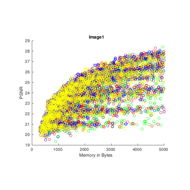
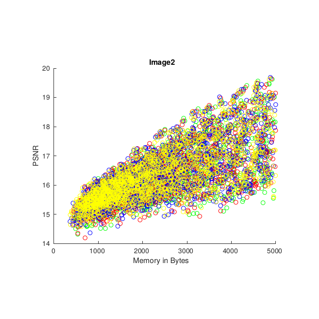
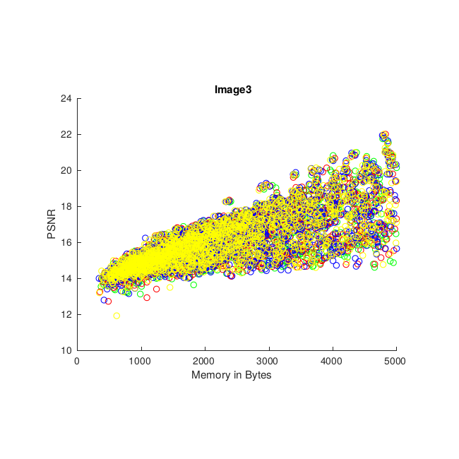
Figure 4. Scatterplots of memory versus PSNR for Image1 (upper left plot), Image2 (upper right plot) and Image3 (lower left plot). Points where blocks varying less than a given threshold have been regarded as constant have been marked with different colours, here green (0), red (15), blue (30) and yellow (45), where the threshold is given within the brackets. The scatterplots indicates that a threshold of 30 is optimal with respect to PSNR and memory, for compression ratios around 150:1, and the optimal threshold tends to decrease with file size.

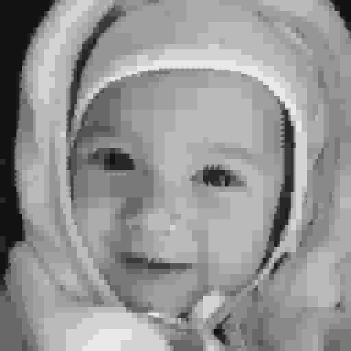
Figure 5. V-variable approximations of Image1 with storage of size 1000 B (PSNR 24.0), 1500 B (PSNR 25.5), 2000 B (PSNR 26.1), and 2500 B (PSNR 26.7).

Figure 6. V-variable approximations of Image2 with storage of size 1500 B (PSNR 16.7), 3000 B (PSNR 18.3), 4500 B (PSNR 19.4), 6000 B (PSNR 20.4).

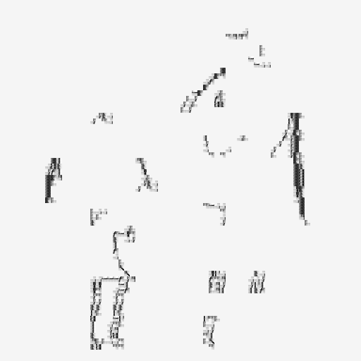
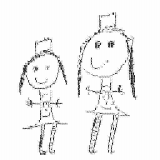
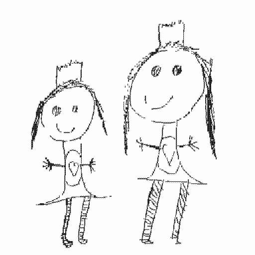
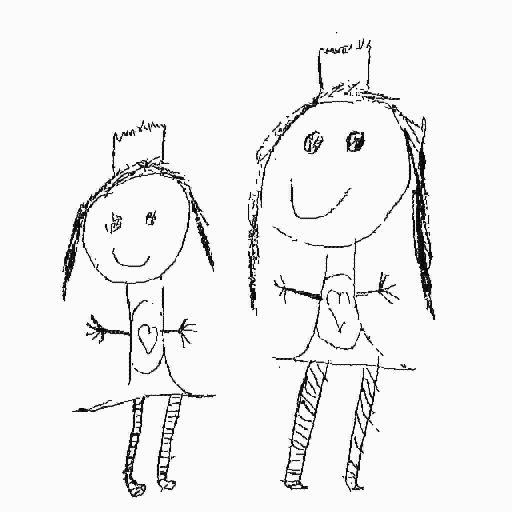
Figure 7. V-variable approximations of Image3 with storage of size 500 B (PSNR 14.6), 1500 B (PSNR 16.5), 2500 B (PSNR 18.4), and 3500 B (PSNR 19.9). The approximating images are rather sharp despite having small PSNR values reflecting the fact that the original image is coloured with two extreme colours and any misprediction at colour boundaries gives a high negative influence on the PSNR.

3. Comparison with other image compression methods

In [3] we discussed compression of the test image here denoted by “Image1” with standard fractal block compression. $\mathbf{V}$-variable compression is slightly better than Fractal compression on Image1 at compression ratios around 100:1 (in the sense of smaller storage size and higher PSNR), and much better on Image2 and Image3. Both Fractal compression and $\mathbf{V}$-variable compression are slow methods with respect to compression time, but decompression is fast.

Fourier and wavelet based methods like JPEG and JP2 works well on photographic images, like Image1, but are not recommended for line art, like Image2 and Image3, where a specialized format like DjVu works much better. JPEG gives roughly the same image quality as $\mathbf{V}$-variable image compression at compression ratios around 100:1 for Image1 and better image quality on Image1 for larger file sizes. It is however worse at all compression levels for Image2 and Image3. This comparison is based on files generated by the free and open source software ImageMagic where we saved the image in JPEG at different quality levels and smaller filesizes than 1.8 KB are then not possible to achieve. One advantage with $\mathbf{V}$-variable compression compared to JPEG is that image quality is not affected by repeated compression. One disadvantage with $\mathbf{V}$-variable compression compared to JPEG is that compression time is slower.

JPEG 2000 gives (based on files generated in ImageMagic) better image quality than $\mathbf{V}$-variable image compression at all compression ratios for Image1 and roughly the same image quality for Image2 at high compression ratios. The image quality is worse than $\mathbf{V}$-variable image compression for Image2 for larger file sizes and worse than $\mathbf{V}$-variable image compression for Image3 at “all” compression ratios.

DjVu is a file format mainly designed for scanned documents that, like $\mathbf{V}$-variable compression, stores images containing a combination of text and line drawings, like Image2 and Image3, well.

It seems like $\mathbf{V}$-variable compression could be a competitive format for intermediate images like digital photos containing line art.

4. Generalisations

4.1. Non-squared images

The general case of a non-squared $j\times k$ image can be treated by e.g. letting $m$ be the smallest integer such that both $j\leq 2^{m}$ and $k\leq 2^{m}$, and consider a square image of size $2^{m}\times 2^{m}$ where the pixelvalue of a given pixel $(a,b)$ in the squared image is given by the pixelvalue of the pixel closest to $(j\cdot a/2^{m},k\cdot b/2^{m})$ in the original image. We then encode the new squared image and transform the resulting image back in the end.

4.2. Clustering methods

The efficiency of our algorithm depends crucially on the clustering method we use. For simplicity in our implementation above we used Matlab’s built-in command kmeans for this step.

There are many approaches to clustering and it is an interesting future problem to explore these in order to find better $\mathbf{V}$-variable approximations than the ones provided by our simple implementation. In particular, the methods used in vector quantization for constructing the codebook could be explored. We can also introduce parameters specifying transformations of image pieces as a pre-processing step before clustering. Matlab also supports “hierarchical clustering” which could have been another simple pre-processing alternative.

4.3. Generalised image pieces

Our definitions of image pieces, and $\mathbf{V}$-variable images can be generalised in various ways. We may define the image pieces as arising from some arbitrary given sequence of refining partitions of a given digital image.

Iterated function systems can be used to recursively define a sequence of refining partitions. Thus the IFS machinery gives us great flexibility in designing recursive partitions and can be used in our scheme. Any periodic self-affine tiling is such an example.

4.4. Reducing the colour space

Reducing the colour space corresponds to chosing the tuple $\mathbf{V}=(V_{1},\ldots,V_{m})$ with $V_{m}$ small. This corresponds to using a colour palette with $V_{m}$ different predetermined colours.

Acknowledgment: We are grateful to Tilo Wiklund for generous assistance and helpful discussions. Franklin Mendivil was partially supported by NSERC (2019-05237).

References

- [1] Barnsley, M. F. and Sloan, A. D. A better way to compress images. Byte 13:215-223, 1988.
- [2] M. F. Barnsley, J. E. Hutchinson and Ö. Stenflo. A fractal valued random iteration algorithm and fractal hierarchy Fractals, 13:111-146, 2005.
- [3] F. Mendivil and Ö. Stenflo. -variable image compression Fractals, 23(02):1550007, 9 pp., 2015.