Recent Developments on Factor Models and its Applications in Econometric Learning

Abstract

This paper makes a selective survey on the recent development of the factor model and its application on statistical learnings. We focus on the perspective of the low-rank structure of factor models, and particularly draws attentions to estimating the model from the low-rank recovery point of view. The survey mainly consists of three parts: the first part is a review on new factor estimations based on modern techniques on recovering low-rank structures of high-dimensional models. The second part discusses statistical inferences of several factor-augmented models and applications in econometric learning models. The final part summarizes new developments dealing with unbalanced panels from the matrix completion perspective.

Key words: factor models, spiked low rank matrix, matrix completion, unbalanced panel, multiple testing, high-dimensional

1 Introduction

The recent decade has witnessed a blossom of developments on statistical learning theories and practice, embraced with the exciting progresses on large-scale optimizations and dimension reduction techniques. Factor models, as one of the central machinery on summarizing and extracting information from large scale datasets, have received much attention in this revolutionary era of data science, and many breakthrough methodologies and applications have been developed in this exciting area.

This paper makes a selective overview on the recent developments of the factor model and its applications on econometric learning. Our review focuses on the perspective of the low-rank structure of factor models, and draws particular attentions to estimating the model from the low-rank recovery point of view. A central focus in the progress of this literature is the understanding and recovering low-rank structures of high-dimensional models. Many new learning theories and methods have been developed, which have revolutionized the modern understanding of econometric modeling. Meanwhile, the low-rank structure is one of the key properties of factor models. While this structure has long been aware of by researchers, studying the factor model from the perspective of low-rank matrix recovery is relatively new, and has led to many exciting new discoveries and understanding.

The survey mainly consists of three parts: the first part is a review on new factor estimation based on modern techniques on recovering low-rank structures of high-dimensional models. The second part discusses statistical inferences of several factor-augmented models and applications in statistical learning models. The final part summarizes new developments dealing with unbalanced panels from the matrix completion perspective.

We concentrate on recent developments on methodologies and applications in econometric learning. For a more comprehensive account on this topic, see Chapters 9-11 of the book by Fan et al. (2020c). Meanwhile, several important topics are not covered in this survey, but have also generated extensive researches in the literature. Those include selecting the number of factors, weak factors, identification, continuous-time and time-varying models, nonstationarity and structural breaks, Bayesian methods, bootstrap factors, as well as more sophisticated panel data models. Several excellent reviews have been written with emphasis on these topics. For those reviews, we refer to Stock and Watson (2016) for dynamic factor models with applications on macroeconomics, to Bai and Wang (2016) for time series and panel data models, and to Gagliardini et al. (2019) for a recent review on conditional factor models with applications to finance. Another class of estimation is a hybrid of PCA-method and the state space approach, see Giannone et al. (2008) and Doz et al. (2011) for more discussions. In addition, the generalized dynamic factor model is another important strand of literature, where factors are often estimated using the dynamic principal components, the frequency domain analog of principal components, developed by Brillinger (1964). Forni et al. (2000, 2005) provided rates of convergence of the common component estimated by dynamic principal components. Finally, we refer to the following papers for more detailed developments, among others: Bai and Ng (2002); Ahn and Horenstein (2013); Onatski (2010); Li et al. (2017), Bai and Li (2012, 2016), Onatski (2012); Chudik et al. (2011), Cheng et al. (2016); Massacci (2017); Gagliardini et al. (2016); Goncalves and Perron (2018); Baltagi et al. (2017); Barigozzi et al. (2018), Aït-Sahalia and Xiu (2017); Chen et al. (2019a); Liao and Yang (2018); Li et al. (2019); Pelger (2019), Su and Wang (2017).

We use the following notation. For a matrix $\mathbf{A}$, let $\lambda_{i}(\mathbf{A})$ denote the $i$ th largest singular value of $\mathbf{A}$ and use $\lambda_{\min}(\mathbf{A})$ and $\lambda_{\max}(\mathbf{A})$ to denote its smallest and largest eigenvalues. We define the Frobenius norm $\|\mathbf{A}\|_{F}=\sqrt{\operatorname{tr}(\mathbf{A}^{\prime}\mathbf{A})}$, the operator norm $\|\mathbf{A}\|=\sqrt{\lambda_{\max}(\mathbf{A}^{\prime}\mathbf{A})}$, the element-wise norm $\|\mathbf{A}\|_{\infty}=\max_{ij}|A_{ij}|$, and the matrix $\ell_{1}$-norm $\|\mathbf{A}\|_{\ell_{1}}:=\max_{i\leq N}\sum_{j=1}^{N}|A_{ij}|$. In addition, define projection matrices $\mathbf{P}_{\mathbf{A}}=\mathbf{A}(\mathbf{A}^{\prime}\mathbf{A})^{-1}\mathbf{A}$ and $\mathbf{M}_{\mathbf{A}}=\mathbf{I}-\mathbf{P}_{\mathbf{A}}$ when $\mathbf{A}^{\prime}\mathbf{A}$ is invertible. Finally, for two (random) sequences $a_{T}$ and $b_{T}$, we write $a_{T}\ll b_{T}$ (or $b_{T}\gg a_{T}$) if $a_{T}=o_{P}(b_{T})$.

2 Spiked Incoherent Low-Rank Models

2.1 The model

Modern high-dimensional factor models can be viewed as a type of spiked incoherent low-rank model, a broad class of models that have drawn active research in the recent decade. A spiked incoherent low-rank model typically refers to a large matrix $\boldsymbol{\Sigma}$ (either observable or not), having the following decomposition:

$$\boldsymbol{\Sigma}=\mathbf{L}+\mathbf{S}.$$ (2.1)

Such decomposition satisfies the following three properties:

(i) Low-rank.

The rank of $\mathbf{L}$ is either bounded or grows very slowly compared to its dimensions.

(ii) Spikedness.

The nonzero singular values of $\mathbf{L}$ grow fast, while the largest singular value of $\mathbf{S}$ is either bounded or grows much slower.

(iii) Incoherence.

(also known as “pervasiveness”) The left and right singular vectors of $\mathbf{L}$, corresponding to the nonzero singular values, should have diversified elements, which means, elements of the rescaled singular vectors should be uniformly bounded.

The low-rank structure achieves dimension reductions: suppose the matrix $\boldsymbol{\Sigma}$ is of $N\times N_{1}$ dimensions, while the rank of $\mathbf{L}$ is $r$. Then the low-rank structure reduces the dimension from $O(NN_{1})$ to $O(N+N_{1})r$; the latter is the magnitude of the number of parameters in $\mathbf{L}$. Meanwhile, the spikedness helps seperate $\mathbf{L}$ from $\mathbf{S}$ approximately, and ensures that the large “signals” concentrate on $\mathbf{L}$, the low rank component. Finally, the incoherence, a condition that excludes matrices being low-rank and sparse simultaneously, enables us to estimate well the singular eigenvectors.

We explain these three properties using the matrix form of factor models. Consider

$$y_{it}=\mathbf{b}_{i}^{\prime}\mathbf{f}_{t}+u_{it},\quad i\leq N,\quad t\leq T,$$ (2.2)

where $\mathbf{f}_{t}$ is a $r$-dimensional vector of factors; $\mathbf{b}_{i}$ is the loading vector and $u_{it}$ is the idiosyncratic noise. Specifically, (2.1) applies to two decompositions of this model.

Factor Decomposition. The matrix form of the factor model gives

$$\mathbf{Y}=\mathbf{M}+\mathbf{U},\quad\mathbf{M}:=\mathbf{B}\mathbf{F}^{\prime},$$

where $\mathbf{Y}$ and $\mathbf{U}$ are $N\times T$ matrices of $y_{it}$ and $u_{it}$; $\mathbf{B}$ is the $N\times r$ matrix of $\mathbf{b}_{i}$ while $\mathbf{F}$ is the $T\times r$ matrix of $\mathbf{f}_{t}.$ Then corresponding to the notation (2.1), $\boldsymbol{\Sigma}=\mathbf{Y}$, $\mathbf{L}=\mathbf{M}$ and $\mathbf{S}=\mathbf{U}.$ In this decomposition, $\boldsymbol{\Sigma}$ is observable. Apparently, $\mathbf{M}$ is a low-rank matrix with rank $r$. The nonzero singular values of $\mathbf{M}$, under the strong factor assumption, grows much faster than those of $\mathbf{U}$, which gives rise to the spikedness property. Now let $\boldsymbol{\xi}$ be the $N\times r$ matrix whose columns are the left singular vectors of $\mathbf{M}$, and let $\boldsymbol{\xi}_{i}^{\prime}$ denote its $i$ th row. Then under the assumption that the nonzero eigenvalues of $\mathbf{B}^{\prime}\mathbf{B}$ grow fast with $N$, for some constant $C>0$,

$$\max_{i\leq N}\|\sqrt{N}\boldsymbol{\xi}_{i}\|\leq C\max_{i\leq N}\|\mathbf{b}_{i}\|,$$ (2.3)

which gives rise to the incoherent singular vectors. The right singular vectors can be bounded similarly.

Covariance Decomposition. It is also well known from the factor model (2.2) that the covariance matrix of $\mathbf{y}_{t}=(y_{1t},\cdots,y_{Nt})^{\prime}$, denoted by $\boldsymbol{\Sigma}_{y}$, can be decomposed as follows:

$$\boldsymbol{\Sigma}_{y}=\mathbf{L}+\boldsymbol{\Sigma}_{u},\quad\mathbf{L}:=\mathbf{B}\operatorname{cov}(\mathbf{f}_{t})\mathbf{B}^{\prime},$$ (2.4)

where $\boldsymbol{\Sigma}_{u}$ denotes the covariance matrix of $\mathbf{u}_{t}$. The above decomposition is well known for portfolio allocations and risk managements, where the total volatility is decomposed into the systematic risk $\mathbf{L}$, plus the (sparse) idiosyncratic risk $\boldsymbol{\Sigma}_{u}$. It also leads to the spiked incoherent low-rank model, but $\boldsymbol{\Sigma}_{y}$ is unknown and needs to be estimated.

2.2 Estimation

There are two general approaches to estimating model (2.1): (i) Principal Components Analysis (PCA), and (ii) low-rank regularization. Here we present a general PCA estimation setting, and defer the discussion of low-rank regularization to Section 3.2. We shall assume rank$(\mathbf{L})=r$ to be known.

For any matrix $\mathbf{A}$, let $\mathbf{A}=\mathbf{U}_{A}\mathbf{D}_{A}\mathbf{V}^{\prime}_{A}$ denote the singular value decomposition (SVD) of $\mathbf{A}$. Define the singular value hard thresholding operator as

$$H_{R}(\mathbf{A}):=\mathbf{U}_{A}\bar{}\mathbf{D}_{R}\mathbf{V}_{A}^{\prime}$$ (2.5)

where $\bar{}\mathbf{D}_{R}$ is a diagonal matrix that keeps the top $R$ diagonal elements of $\mathbf{D}_{A}$ and replaces the remaining elements by zeros. So $H_{R}(\mathbf{A})$ is the best rank $R$ matrix approximation to $\mathbf{A}$.

Suppose an estimator of $\boldsymbol{\Sigma}$, denoted by $\widehat{}\boldsymbol{\Sigma}$, is available, satisfying

$$\|\widehat{}\boldsymbol{\Sigma}-\boldsymbol{\Sigma}\|=O_{P}(\eta_{N}),\quad\|\widehat{}\boldsymbol{\Sigma}-\boldsymbol{\Sigma}\|_{\infty}=O_{P}(c_{N})$$ (2.6)

for some sequences $\eta_{N}$ and $c_{N}$. We use $\widehat{}\boldsymbol{\Sigma}$ as the input matrix, which can be the sample covariance matrix or its robustfied versions (Fan et al., 2019c). The goal is to estimate $\mathbf{L}$ in (2.1) and its $N\times r$ matrix of the left singular vectors, denoted by $\boldsymbol{\xi}$ (also let $\boldsymbol{\zeta}$ denote its right singular vectors). We use respectively $\widehat{}\mathbf{L}:=H_{R}(\widehat{}\boldsymbol{\Sigma})$ with $R=r$, which is the rank $r$ projection of $\widehat{\boldsymbol{\Sigma}}$, and the $N\times r$ matrix $\widehat{}\boldsymbol{\xi}$ whose columns are the left singular vectors of $\widehat{}\boldsymbol{\Sigma}$. The following theorem, adapted from Fan et al. (2018), provides deviation bounds of the estimators. To make the paper self-contained, we also provide a simpler proof with slightly different conditions.

Theorem 2.1.

Consider the general model (2.1) with bounded $r:=\text{rank}(\mathbf{L})$. Suppose that $\min_{2\leq i\leq r+1}|\lambda_{i-1}(\mathbf{L})-\lambda_{i}(\mathbf{L})|\asymp\max_{2\leq i\leq r+1}|\lambda_{i-1}(\mathbf{L})-\lambda_{i}(\mathbf{L})|:=g_{N}$ and $\eta_{N}+\|\mathbf{S}\|=o_{P}(g_{N})$. Then, under condition (2.6), we have (i)

$$\|\widehat{}\mathbf{L}-\mathbf{L}\|=O_{P}\left(\eta_{N}+\|\mathbf{S}\|\right),\quad\|\widehat{}\boldsymbol{\xi}-\boldsymbol{\xi}\|=O_{P}\left(\frac{\eta_{N}+\|\mathbf{S}\|}{g_{N}}\right).$$

(ii) If additionally, $\|\mathbf{S}\|_{\infty}+\|\mathbf{L}\|_{\infty}=O_{P}(1)$, $N_{1}c_{N}=o_{P}(g_{N})$, then

$$\|\widehat{}\boldsymbol{\xi}-\boldsymbol{\xi}\|_{\infty}\leq O_{P}\left(\frac{N_{1}}{\sqrt{N}}+\sqrt{N_{1}}\right)(\eta_{N}+\|\mathbf{S}\|)g_{N}^{-2}$$

$$\qquad+O_{P}\left(c_{N}\frac{N_{1}}{\sqrt{N}}+c_{N}\sqrt{N_{1}}+\|\mathbf{S}\boldsymbol{\zeta}_{d}\|_{\infty}\vee\|\mathbf{S}^{\prime}\boldsymbol{\xi}_{d}\|_{\infty}\right)g_{N}^{-1}.$$

Proof.

See the online supplement. ∎

This theorem is relatively general, and is applicable to low-rank models that are not necessarily consequences from factor models. The proof relies on perturbation bounds for singular vectors/values, and the achieved rates are sharp. Result (i) is simple and gives asymptotic bounds under the operator norm. Result (ii) gives element-wise deviation bound for the singular vectors, which requires more dedicated technical arguments.

3 Estimation under Factor Models

We observe an $N\times T$ data matrix $\mathbf{Y}$, which can be decomposed as

$$\mathbf{Y}=\mathbf{M}+\mathbf{U}=\mathbf{B}\mathbf{F}^{\prime}+\mathbf{U}$$

where $\mathbf{B}$ is $N\times r$ factor loadings matrix, $\mathbf{F}$ is $T\times r$ factors matrix and $\mathbf{U}$ is $N\times T$ idiosyncratic errors, which are uncorrelated with $\mathbf{M}:=\mathbf{B}\mathbf{F}^{\prime}$. All the three parts $\mathbf{B}$, $\mathbf{F}$ and $\mathbf{U}$ are unobserved. The $t$ th column of this expression can be written as

$$\mathbf{y}_{t}=\mathbf{B}\mathbf{f}_{t}+\mathbf{u}_{t}.$$ (3.1)

3.1 PCA and MLE

3.1.1 PCA

Under the model’s specification, we have the covariance structure (2.4). One of the most widely used estimation methods for the factor model is principal components analysis (PCA). Define the sample covariance $\mathbf{S}_{y}=\frac{1}{T}\sum_{t=1}^{T}\mathbf{y}_{t}\mathbf{y}_{t}^{\prime}=\frac{1}{T}\mathbf{Y}\mathbf{Y}^{\prime}$. Let $\widehat{}\boldsymbol{\xi}_{j}$ be the $j$th eigenvector corresponding to the largest $j$ th eigenvalues of $\mathbf{S}_{y}$. The PCA estimates $\mathbf{B}$ by taking $\widehat{}\mathbf{B}=\sqrt{N}(\widehat{}\boldsymbol{\xi}_{1},\cdots,\widehat{}\boldsymbol{\xi}_{R})$, which estimates $\mathbf{B}$ up to a diagonal transformation. Given $\widehat{}\mathbf{B}$, the factors can be estimated via the least squares:

$$\widehat{}\mathbf{F}=\mathbf{Y}^{\prime}\widehat{}\mathbf{B}(\widehat{}\mathbf{B}^{\prime}\widehat{}\mathbf{B})^{-1}=\frac{1}{N}\mathbf{Y}^{\prime}\widehat{}\mathbf{B}.$$

This also leads to the estimated low-rank component $\frac{1}{T}\widehat{}\mathbf{B}\widehat{}\mathbf{F}^{\prime}\widehat{}\mathbf{F}\widehat{}\mathbf{B}^{\prime}$ for $\mathbf{B}\operatorname{cov}(\mathbf{f}_{t})\mathbf{B}^{\prime}$.

PCA is equivalent to the singular value hard thresholding by taking the input matrix $\widehat{}\boldsymbol{\Sigma}=\mathbf{S}_{y}$. Then $\frac{1}{T}\widehat{}\mathbf{B}\widehat{}\mathbf{F}^{\prime}\widehat{}\mathbf{F}\widehat{}\mathbf{B}^{\prime}=H_{R}(\mathbf{S}_{y})$. One can then apply Theorem 2.1 to infer the rates of convergence of the PCA estimators, which were obtained by Stock and Watson (2002a). Bai (2003) proved the asymptotic normality of PCA estimators for the factors and loadings. Results with general input $\widehat{\boldsymbol{\Sigma}}$ can be found in Chapter 10 of Fan et al. (2020c).

3.1.2 Maximum Likelihood Estimations

Another popular method to estimate a factor model is the maximum likelihood (ML) method (see, e.g., Lawley and Maxwell (1971), Bai and Li (2012), Doz et al. (2012)). Under the independence and normality assumptions, the log-likelihood function based on $\mathbf{y}_{t}$ is, for some constant $C$,

$$\log L_{\mathrm{ML}}(\mathbf{B},\operatorname{cov}(\mathbf{f}_{t}),\operatorname{diag}(\boldsymbol{\Sigma}_{u}))=C-\frac{T}{2}\ln|\boldsymbol{\Sigma}_{y}|-\frac{1}{2}\sum_{t=1}^{T}\mathbf{y}_{t}^{\prime}\boldsymbol{\Sigma}_{y}^{-1}\mathbf{y}_{t}.$$

The log-likelihood function is then maximized with respect to the matrix parameters $(\mathbf{B},\operatorname{cov}(\mathbf{f}_{t}),\operatorname{diag}(\boldsymbol{\Sigma}_{u}))$ under additional restrictions that $\boldsymbol{\Sigma}_{u}$ is diagonal (Bai and Li, 2012, 2016) or sparse with regularizations (Bai and Liao, 2016; Wang et al., 2019b). Recently Barigozzi and Luciani (2019) explicitly accounted for autocorrelations of the factors in the likelihood function.

The factors can be estimated by two methods, one of which is the projection method. Under the joint normality assumptions of $\mathbf{f}_{t}$ and $\mathbf{u}_{t}$, we have

$$\mathbb{E}(\mathbf{f}_{t}|\mathbf{y}_{t})=\mathbf{B}^{\prime}(\mathbf{B}\mathbf{B}^{\prime}+\boldsymbol{\Sigma}_{u})^{-1}\mathbf{y}_{t}=(\mathbf{I}_{r}+\mathbf{B}^{\prime}\boldsymbol{\Sigma}_{u}^{-1}\mathbf{B})^{-1}\mathbf{B}^{\prime}\boldsymbol{\Sigma}_{u}^{-1}\mathbf{y}_{t}.$$

This provides the basis of estimating factors. The other approach is the generalized least squares: for given $\mathbf{B}$ and $\boldsymbol{\Sigma}_{u}^{-1}$, the GLS estimator for $\mathbf{f}_{t}$ is

$$\widehat{}\mathbf{f}_{t}=(\mathbf{B}^{\prime}\boldsymbol{\Sigma}_{u}^{-1}\mathbf{B})^{-1}\mathbf{B}^{\prime}\boldsymbol{\Sigma}_{u}^{-1}\mathbf{y}_{t}.$$

Replacing the unknown parameters with their ML estimators, one obtains two estimators for the latent factors. Under large-$N$ setup, the difference of the two methods (PCA and MLE) for estimating factors are asymptotically negligible.

3.2 Low rank estimation

Alternative to PCA, one can estimate $\mathbf{M}$ directly taking advantage of its low-rank structure, based on the nuclear-norm regularization, the $\ell_{1}$-norm of singular values, that encourages the sparseness in singular values and hence low-rankness. For an $n\times m$ matrix $\mathbf{A}$, let $\|\mathbf{A}\|_{n}:=\sum_{i=1}^{\min\{m,n\}}\psi_{i}(\mathbf{A})$ be its nuclear-norm, where $\psi_{i}(\mathbf{A})$ is the $i$ th largest singular value of $\mathbf{A}$.

3.2.1 Singular value thresholding

Given the low-rank structure of $\mathbf{M}$ (sparsity in singular value of $\mathbf{M}$), we can estimate the model via solving the following penalized optimization:

$$\widehat{}\mathbf{M}=\arg\min_{M}\frac{1}{2}\|\mathbf{Y}-\mathbf{M}\|_{F}^{2}+\nu\|\mathbf{M}\|_{n}$$ (3.2)

for some tuning parameter $\nu>0$. The solution is $\widehat{}\mathbf{M}=S_{\nu}(\mathbf{Y})$, where $S_{\nu}(\cdot)$ is the singular value thresholding operator (Ma et al., 2011), defined as follows. Let $\mathbf{Y}=\mathbf{U}_{y}\mathbf{D}\mathbf{V}_{y}^{\prime}$ be its SVD. Then $S_{\nu}(\mathbf{Y}):=\mathbf{U}_{y}\mathbf{D}_{\nu}\mathbf{V}_{y}^{\prime},$ where $\mathbf{D}_{\nu}=\operatorname{diag}(\{D_{ii}-\nu\}_{+})$ with $D_{ii}$ being the diagonal entries of $\mathbf{D}$. So $S_{\nu}(\mathbf{Y})$ applies “soft-thresholding” on the singular values of $\mathbf{Y}$. One can additionally estimate the factors and loadings using the singular vectors.

We note that this method is closely related to the PC-estimator, except the soft-thresholding is replaced by hard-threshoding. Let $R$ denote the “working number of factors”, which is the number of principal components one takes when applying the PC-method. We note that the PC-estimator for $\mathbf{M}$ with $R$ factors is given by (see Section 2.2):

$$\widehat{}\mathbf{M}_{\text{PC}}=H_{R}(\mathbf{Y}),\quad H_{R}(\mathbf{Y}):=\mathbf{U}_{y}\bar{}\mathbf{D}_{R}\mathbf{V}_{y}^{\prime}.$$

This estimator is the solution to the penalized least squares problem (3.2) except that the nuclear norm is replaced by $\sum_{i=1}^{\min\{N,T\}}p_{\nu}(\psi_{i}(\mathbf{M}))$, where $p_{\nu}(\theta)=\nu^{2}-(\nu-|\theta|)_{+}^{2}$ is the harding thresholding penalty and $\psi_{i}(\mathbf{M})$ is the $i^{th}$ singular value of $\mathbf{M}$.

Therefore the difference between (3.2) and PCA is more fundamentally about that of hard- and soft- thresholding. Despite of many good properties, the soft-thresholding estimator possesses shrinkage bias, while the hard-thresholding reduces the bias. As a matter of fact, the shrinkage bias is on the singular values, rather than on the singular vectors. Indeed, the singular vectors of the two estimators are the same, and equal to the top $R$ singular vectors of $\mathbf{Y}.$ An important implication is that the factor estimator building on $\widehat{}\mathbf{M}$ is numerically equivalent to the PC-estimators for the factors, which does not suffer from any shrinkage bias. A formal statement and proof of the unbiasedness of eigenvectors can be found in Fan et al. (2019b).

3.2.2 Low-rank plus sparse decomposition

Recall that $\boldsymbol{\Sigma}_{y}$ and $\boldsymbol{\Sigma}_{u}$ denote the $N\times N$ covariance matrices of $\mathbf{y}_{t}$ and $\mathbf{u}_{t}$ in model (3.1), and that we have the following decomposition

$$\boldsymbol{\Sigma}_{y}=\mathbf{L}+\boldsymbol{\Sigma}_{u},\quad\mathbf{L}:=\mathbf{B}\operatorname{cov}(\mathbf{f}_{t})\mathbf{B}^{\prime}.$$ (3.3)

We now demonstrate that this decomposition also provides a nice structure for estimating the covariance components. A key assumption is conditionally sparsity, namely, $\boldsymbol{\Sigma}_{u}$ is sparse. While the definition of sparsity may differ in different contexts, here we mean

$$J:=\sum_{i\neq j}1\{\operatorname{\mathbb{E}}u_{it}u_{jt}\}$$

should not grow too fast as $N\to\infty.$ This requirement can be weakened to approximate sparsity. In addition, $\mathbf{L}$ is a low-rank matrix. Thus we can directly estimate the above covariance decomposition via solving the following penalized optimization:

$$(\widehat{}\mathbf{L},\widehat{}\boldsymbol{\Sigma}_{u}):=\arg\min_{\mathbf{L},\boldsymbol{\Sigma}_{u}}\frac{1}{2}\|\mathbf{S}_{y}-(\mathbf{L}+\boldsymbol{\Sigma}_{u})\|_{F}^{2}+\nu_{1}\|\mathbf{L}\|_{n}+\nu_{2}\|\boldsymbol{\Sigma}_{u}\|_{1},$$ (3.4)

where $\nu_{1}$ and $\nu_{2}$ are tuning parameters. Note that here we use the notation $\|\mathbf{A}\|_{1}=\sum_{i,j}|A_{ij}|$ as the matrix 1-norm, distinguished from the usual matrix $\ell_{1}$-norm $\|\mathbf{A}\|_{\ell_{1}}:=\max_{i\leq N}\sum_{j=1}^{N}|A_{ij}|$. The above optimization has been employed by many authors to study the low rank plus sparse decomposition, while some authors exclude the diagonal elements of $\boldsymbol{\Sigma}_{u}$ from the penalization, and additionally impose positive-definite and other constraints on $\mathbf{L}$ and $\boldsymbol{\Sigma}_{u}$ (Klopp et al., 2017; Agarwal et al., 2012). Finally, given $\widehat{}\mathbf{L}$, we can estimate the factors and loadings by extracting its eigenvectors.

The above optimization can be solved by alternating the estimation of $\mathbf{L}$ and $\boldsymbol{\Sigma}_{u}$, and closed form solutions are available in both iterations. Given $\boldsymbol{\Sigma}_{u}$, solving for $\mathbf{L}$ leads to the singular value soft-thresholding: $\widehat{\mathbf{L}}=S_{\nu_{1}}(\mathbf{S}_{y}-\boldsymbol{\Sigma}_{u})$, and given $\mathbf{L}$, solving for $\boldsymbol{\Sigma}_{u}$ leads to the element-wise soft-thresholding: $\widehat{\boldsymbol{\Sigma}}_{u}=\widetilde{S}_{\nu_{2}}(\mathbf{S}_{y}-\mathbf{L})$. While both iterations solve convex problems, standard convergence analysis can be applied to show that the iterative algorithm converges in polynomial time.

Agarwal et al. (2012) and Klopp et al. (2017) studied the statistical convergence properties of (3.4). Let columns of $\mathbf{U}_{L,2}$ be the singular vectors of the true $\mathbf{L}$ corresponding to the zero singular values. Define projections $\mathcal{P}(\mathbf{A}):=\mathbf{U}_{L,2}\mathbf{U}_{L,2}^{\prime}\mathbf{A}\mathbf{U}_{L,2}\mathbf{U}_{L,2}^{\prime}$ and $\mathcal{M}(\mathbf{A}):=\mathbf{A}-\mathcal{P}(\mathbf{A})$. In addition, let $(\mathbf{A})_{J}$ and $(\mathbf{A})_{J^{c}}$ be the submatrices of $\mathbf{A}$, whose elements respectively correspond to $\operatorname{\mathbb{E}}u_{it}u_{jt}\neq 0$ and $\operatorname{\mathbb{E}}u_{it}u_{jt}=0.$ Additionally define

$$\mathcal{C}(\nu_{1},\nu_{2}):=\{(\mathbf{A}_{1},\mathbf{A}_{2}):\nu_{1}\|\mathcal{P}(\mathbf{A}_{1})\|_{n}+\nu_{2}\|(\mathbf{A}_{2})_{J^{c}}\|_{1}\leq 3\nu_{1}\|\mathcal{M}(\mathbf{A}_{1})\|_{n}+3\nu_{2}\|(\mathbf{A}_{2})_{J}\|_{1}\}.$$

A key quantity is the restricted strong convexity (RSC) constant, which is defined as follows:

$$\kappa(\nu_{1},\nu_{2}):=\sup\{c>0:\|\mathbf{A}_{1}+\mathbf{A}_{2}\|_{F}^{2}\geq c\|\mathbf{A}_{1}\|_{F}^{2}+c\|\mathbf{A}_{2}\|_{F}^{2}\text{ for all }(\mathbf{A}_{1},\mathbf{A}_{2})\in\mathcal{C}(\nu_{1},\nu_{2})\}.$$

We then have the following theorem, adapted from Agarwal et al. (2012). To make the paper self-contained, we also provide a proof with slightly different conditions. See the online supplement.

Theorem 3.1.

Conditioning on events $4\|\mathbf{S}_{y}-\boldsymbol{\Sigma}_{y}\|\leq\nu_{1}$ and $4\|\mathbf{S}_{y}-\boldsymbol{\Sigma}_{y}\|_{\infty}\leq\nu_{2}$, there is $C>0$ that only depends on $\text{rank}(\mathbf{L})$, so that

$$\frac{1}{N^{2}}\|\widehat{}\mathbf{L}-\mathbf{L}\|_{F}^{2}+\frac{1}{N^{2}}\|\widehat{}\boldsymbol{\Sigma}_{u}-\boldsymbol{\Sigma}_{u}\|_{F}^{2}\leq\frac{C}{\kappa^{2}(\nu_{1},\nu_{2})}\frac{(\nu_{1}^{2}+(J+N)\nu_{2}^{2})}{N^{2}}.$$

Proof.

See the online supplement. ∎

The optimal tuning parameters can be set to satisfy $\nu_{1}\asymp\frac{N}{\sqrt{T}}$ and $\nu_{2}\asymp\sqrt{\frac{\log N}{T}}$, respectively, accounting for estimating errors under two matrix norms:

$$\|\mathbf{S}_{y}-\boldsymbol{\Sigma}_{y}\|\leq\nu_{1},\quad\|\mathbf{S}_{y}-\boldsymbol{\Sigma}_{y}\|_{\infty}\leq\nu_{2};$$

both can be shown to hold with high probability under weak serial dependence and sub-Gaussian conditions. In additionally, if $\kappa(\nu_{1},\nu_{2})$ is bounded away from zero, with the choice of tunings, the convergence rate in Theorem 3.1 is $O_{P}(1+\frac{J\log N}{N^{2}})\frac{1}{T}$, which is sufficient to guarantee the convergence of the estimated factors and loadings. We refer to Lemma 2 of Agarwal et al. (2012) for more refined lower bound of $\kappa(\nu_{1},\nu_{2})$.

The above problem is also called “robust PCA” (Candès et al., 2011). For recent advance and references, see Chen et al. (2020c) where factorization methods are also discussed.

3.3 Covariance estimation

Fan et al. (2013) proposed a nonparametric estimator of $\boldsymbol{\Sigma}_{y}$, named POET (Principal Orthogonal complEment Thresholding), when the factors are unobservable. It is basically an one-step solution to optimization (3.4) with initialization $\boldsymbol{\Sigma}_{u}=0$. To motivate the estimator, suppose $r=R$. Then, heuristically

$$\mathbf{L}\approx H_{R}(\boldsymbol{\Sigma}_{y}),\quad\boldsymbol{\Sigma}_{u}\approx\boldsymbol{\Sigma}_{y}-H_{R}(\boldsymbol{\Sigma}_{y}),$$

Thus, one estimates $\mathbf{L}$ by $H_{R}(\mathbf{S}_{y})$ and sets $\mathbf{S}_{u}:=\mathbf{S}_{y}-H_{R}(\mathbf{S}_{y})$. To account for the sparsity assumption on $\boldsymbol{\Sigma}_{u}$, Fan et al. (2013) estimates $\boldsymbol{\Sigma}_{y}$ and $\boldsymbol{\Sigma}_{u}$ as

$$\widehat{}\boldsymbol{\Sigma}_{y}=H_{R}(\mathbf{S}_{y})+\widehat{}\boldsymbol{\Sigma}_{u},\quad\widehat{}\boldsymbol{\Sigma}_{u}=(h(S_{u,ij},\lambda_{ij}))_{N\times N},$$ (3.5)

where $h(x,\lambda_{ij})$ denotes the element-wise thresholding operator with thresholding value $\lambda_{ij}$. Here, we emphasize element-dependent thresholding $\lambda_{ij}$ to adapt to varying scales of covariance. For correlation thresholding at level $\lambda$, we take $\lambda_{ij}=\lambda\sqrt{s_{u,ii}s_{u,jj}}$ with $s_{u,ii}$ a diagnonal element of $\mathbf{S}_{u}$(Fan et al., 2013); we can also take other form such as the adaptive thresholding in Cai and Liu (2011). In general, the thresholding function should satisfy:
(i) $h(x,\lambda)=0$ if $|x|<\lambda$,
(ii) $|h(x,\lambda)-x|\leq\lambda$.
(iii) there are constants $a>0$ and $b>1$ such that $|h(x,\lambda)-x|\leq a\lambda^{2}$ if $|x|>b\lambda$.

Note that condition (iii) requires that the thresholding bias should be of higher order. It is not necessary for consistent estimations, but we recommend using nearly unbiased thresholding (Antoniadis and Fan, 2001) for inference applications. One such example is known as SCAD. As noted in Fan et al. (2015), the unbiased thresholding is required to avoid size distortions in a large class of high-dimensional testing problems involving a “plug-in” estimator of $\boldsymbol{\Sigma}_{u}$. In particular, this rules out the popular soft-thresholding function, which does not satisfy (iii) due to its first-order shrinkage bias.

3.4 Projected PCA

In empirical asset pricing, factor loadings are known to depend on individual-specific observables $\mathbf{X}_{i}$, which represent a set of time-invariant characteristics such as individual stocks’ size, momentum, and values. To incorporate the information carried by the observed characteristics, Connor and Linton (2007) and Connor et al. (2012) model explicitly the loading matrix as a function of covariates $\mathbf{X}_{i}$. Fan et al. (2016) extended the model to allowing components in factor loadings that are not explainable by characteristics:

$$\mathbf{b}_{i}=\mathbf{g}(\mathbf{X}_{i})+\boldsymbol{\gamma}_{i},\quad\operatorname{\mathbb{E}}(\boldsymbol{\gamma}_{i}|\mathbf{X}_{i})=0.$$ (3.6)

Here $\mathbf{g}(\cdot)$ is a vector of nonparametric functions. With this model, they introduced an improved factor estimator, known as projected PCA.

The basic idea of projected PCA is to smooth the observations $\{y_{it}\}_{i=1}^{N}$ for each given $t$ against their associated covariates $\{\mathbf{X}_{i}\}_{i=1}^{N}$ (cross-sectional smoothing), and apply PCA to the smoothed data (fitted values). Let $\{\phi_{j}(\mathbf{x})\}_{j=1}^{J}$ be a set of basis functions. This can be either unstructured, such as kernel machines, or structured such as a basis for additive models (Fan et al., 2020c). Set $\phi(\mathbf{X}_{i})^{\prime}=(\phi_{1}(\mathbf{X}_{i}),\cdots.,\phi_{J}(\mathbf{X}_{i}))$ and $\Phi(\mathbf{X})=(\phi(\mathbf{X}_{1}),\cdots,\phi(\mathbf{X}_{N}))^{\prime}$, an $N\times J$ matrix. Then the projection matrix on characteristics can be taken as $\mathbf{P}=\Phi(\mathbf{X})(\Phi(\mathbf{X})^{\prime}\Phi(\mathbf{X}))^{-1}\Phi(\mathbf{X})^{\prime}.$ The projected data $\mathbf{P}\mathbf{Y}$ is the fitted value of regressing $\mathbf{Y}$ on to the basis functions.

We make the following key assumptions:

Assumption 3.1.

(i) Relevance:

With probability approaching one, all the eigenvalues of $\frac{1}{N}({\mathbf{P}}\mathbf{B})^{\prime}{\mathbf{P}}\mathbf{B}$ are bounded away from both zero and infinity as $N\to\infty$.

(ii) Orthogonality:

$\mathbb{E}(u_{it}|\mathbf{X}_{i})=0$ for all $i\leq N,t\leq T.$

The above conditions require that the strengths of the loading matrix should remain strong after the projection. Condition (ii) implies that if we apply $\mathbf{P}$ to both sides of $\mathbf{Y}=\mathbf{B}\mathbf{F}^{\prime}+\mathbf{U}$, then

$$\mathbf{P}\mathbf{Y}\approx\mathbf{P}\mathbf{B}\mathbf{F}^{\prime}=\mathbf{G}\mathbf{F}^{\prime}$$

where $\mathbf{G}=\mathbf{P}\mathbf{B}$ is the $N\times r$ matrix, which $\approx(\mathbf{g}(\mathbf{X}_{i}))_{N\times r}$ under additional assumption $\operatorname{\mathbb{E}}(\boldsymbol{\gamma}_{i}|\mathbf{X}_{i})=0$ for all $i\leq N$. In other words, the noise $\mathbf{U}$ is suppressed, while signals remain. Hence, the scaled sample covariance $(\mathbf{P}\mathbf{Y})^{\prime}\mathbf{P}\mathbf{Y}=\mathbf{Y}^{\prime}\mathbf{P}\mathbf{Y}\approx\mathbf{F}\mathbf{G}^{\prime}\mathbf{G}\mathbf{F}^{\prime}.$ For identification purpose, let us assume $\boldsymbol{\Xi}:=\mathbf{G}^{\prime}\mathbf{G}$ is a diagonal matrix and $\mathbf{F}^{\prime}\mathbf{F}/T=\mathbf{I}$. Then from

$$\frac{1}{T}\mathbf{Y}^{\prime}\mathbf{P}\mathbf{Y}\mathbf{F}\approx\mathbf{F}\boldsymbol{\Xi},$$

we infer that the columns of $\mathbf{F}$ are approximately the eigenvectors of the $\mathbf{Y}^{\prime}\mathbf{P}\mathbf{Y}$, scaled by a factor $\sqrt{T}$. This motivates estimating factors by using the top $R$ eigenvectors of $\mathbf{Y}^{\prime}\mathbf{P}\mathbf{Y}$.

Fan et al. (2016) derived the rates of convergence of the projected PCA method. A nice feature is that the consistency of latent factors is achieved even when the sample size $T$ is finite so long as $N$ goes to infinity. Intuitively, the idiosyncratic noise is removed from cross-sectional projections, which does not require a long time series.

Similarly, in many applications, while we do not know the latent factors $\mathbf{f}_{t}$, we do know that factors are related to some proxy variables $\mathbf{W}_{t}$. For example, the latent factors are unknown for equity markets, but they are related to Fama-French factors (Fama and French, 2015); latent factors for disaggregated macroeconomics time series are unknown, but they are related to aggregated ones (McCracken and Ng, 2016). Switching the roles of rows and columns, longitudinal regression of each series $\{y_{it}\}_{t=1}^{T}$ on $\{\mathbf{W}_{t}\}_{t=1}^{T}$ yields the projected data matrix, from which latent factors and loadings can be extracted similarly. See Fan et al. (2020a) for details on how latent factor learning is augmented by instruments $\{\mathbf{W}_{t}\}_{t=1}^{T}$.

3.5 Diversified projection

In this section, we continue denoting by $R$ as the number of factors we use, and by $r$ as the true number of factors. Fan and Liao (2020) proposed a simpler factor estimator that does not rely on eigenvectors, by using cross-sectional diversified projections (DP). Let $\mathbf{W}=(\mathbf{w}_{1},\cdots,\mathbf{w}_{R})$ be a given exogenous (or deterministic) $N\times R$ matrix, where each of its $R$ columns $\mathbf{w}_{k}$ is an $N\times 1$ vector of “diversified weights”, whose definition is to be clear below. We estimate $\mathbf{f}_{t}$ by simply taking

$$\widehat{}\mathbf{f}_{t}=\frac{1}{N}\mathbf{W}^{\prime}\mathbf{y}_{t}.$$

By substituting $\mathbf{y}_{t}=\mathbf{B}\mathbf{f}_{t}+\mathbf{u}_{t}$ into the definition, immediately we have

$$\widehat{}\mathbf{f}_{t}=\mathbf{H}\mathbf{f}_{t}+\frac{1}{N}\mathbf{W}^{\prime}\mathbf{u}_{t},\quad\mathbf{H}=\frac{1}{N}\mathbf{W}^{\prime}\mathbf{B}.$$ (3.7)

Thus $\widehat{}\mathbf{f}_{t}$ (consistently) estimates $\mathbf{f}_{t}$ up to an $R\times r$ affine transform $\mathbf{H}$, with the estimation error $\mathbf{e}_{t}:=\frac{1}{N}\mathbf{W}^{\prime}\mathbf{u}_{t}$. The assumption that $\mathbf{W}$ should be diversified ensures that as $N\to\infty$, $\mathbf{e}_{t}$ is “diversified away” (converging to zero in probability). More specifically, we impose the following assumption.

Assumption 3.2.

There is a constant $c>0$, so that as $N\to\infty$,
(i) The $R\times R$ matrix $\frac{1}{N}\mathbf{W}^{\prime}\mathbf{W}$ satisfies $\lambda_{\min}(\frac{1}{N}\mathbf{W}^{\prime}\mathbf{W})>c.$
(ii) $\mathbf{W}$ is independent of $\{\mathbf{u}_{t}:t\leq T\}$.
(iii) Suppose $R\geq r$, $\operatorname{rank}(\mathbf{H})=r$ and $\psi^{2}_{\min}(\mathbf{H})\gg\frac{1}{N}$, where $\psi_{\min}(\mathbf{H})$ denotes the minimum nonzero singular value of $\mathbf{H}=\frac{1}{N}\mathbf{W}^{\prime}\mathbf{B}$.

Conditions (i) and (ii) define the “diversified weights” $\mathbf{W}$. When $(u_{1t},\cdots,u_{Nt})$ are cross-sectionally weakly dependent, they ensure that $\mathbf{e}_{t}$ is diversified away. Condition (iii) of Assumption 3.2 is a key condition, which requires that $\mathbf{W}$ should not diversify away the factor components in the time series. Several choices of $\mathbf{W}$ can be recommended to satisfy this condition. For instance, if factor loadings satisfy (3.6), then fix $R$ components of sieve basis functions: $(\phi_{1}(\cdot),\cdots,\phi_{R}(\cdot))$, we can define

$$\mathbf{W}:=(w_{i,k})_{N\times R},\quad\text{ where }w_{i,k}=\phi_{k}(\mathbf{X}_{i}).$$

Alternatively, we can also use transformations of the initial observation $\mathbf{x}_{t}$ for $t=0$, which was considered by Juodis and Sarafidis (2020). If $\mathbf{y}_{0}$ is independent of $\{\mathbf{u}_{t}:t\geq 1\}$, we can apply $w_{i,k}=\phi_{k}(y_{i,0})$ . These weights are correlated with $\mathbf{B}$ through $\mathbf{y}_{0}=\mathbf{B}\mathbf{f}_{0}+\mathbf{u}_{0}$.

An important benefit of the DP is that it is robust to over-estimating the number of factors. Theoretical studies of factor models have been crucially depending on the assumption that the number of factors, $r$, should be consistently estimated. This usually requires strong conditions on the strength of factors and serial conditions. Recently, Barigozzi and Cho (2018) proposed a PCA-based method to estimate factors that are robust to over-estimated $r$. They provided rates of convergence of the estimated common components when $R\geq r$.

Fan and Liao (2020) applied DP to several inference problems in factor-augmented models, including the post-selection inference, high-dimensional covariance estimation, and factor specification tests. They formally justified the robustness to over-estimating the number of factors in these applications. In particular, DP admits $r=0$ but $R\geq 1$ as a special case. That is, the inference is still valid even if there are no common factors present, but factors are nevertheless estimated for insurance. In addition, Karabiyik et al. (2019) applied DP to the context of panel data models in the presence of common factors.

3.6 Factor estimators robust to heavy tails

To apply either the PCA or the MLE to estimate the model, we need an initial covariance estimator $\mathbf{S}_{y}$, whose application requires elements of $\mathbf{y}_{t}$ have sufficient moments. Some technical results of factor estimations even require sub-Gaussian conditions on data’s tail distributions. However, heavy tailed data are not uncommon in economic applications. For instance, about thirty percent of 131 disaggregated macroeconomic variables of Ludvigson and Ng (2016) have excess kurtosis greater than six, so their distributions are fatter than the t-distribution with degrees of freedom five. Indeed, heavy tails are a stylized feature of high-dimensional data, as it is unlikely that all variables have sub-Gaussian tails.

Because the presence of heavy-tailed data invalidates many conditions required for estimating factor models, the recent literature has proposed several methods that are robust to the tail distributions. Here we describe two of them: truncation and robust M-estimation.

In the high-dimensional setting, consider estimating multivariate means from an independent triangular array variables $y_{i1},...,y_{iT}$ with $\max_{i\leq N}\operatorname{Var}(y_{it})\leq\sigma^{2}$. Truncate the data

$$\widetilde{y}_{it}:=\mbox{sgn}(y_{it})\min\{|y_{it}|,\tau_{i}\}$$

with predetermined $\tau_{i}>0$. We then estimate $\mathbb{E}y_{it}$ using the truncated-mean $\widetilde{y}_{i}:=\frac{1}{T}\sum_{t=1}^{T}\widetilde{y}_{it}$. Theorem 3.2 shows that the high-dimensional means can be estimated uniformly well if $\mathbb{E}|y_{it}|^{q}<M$ for some $q\geq 2$.

Catoni (2012) constructed a robust M-estimator that shares the same Gaussian concentration. Fan et al. (2017a, 2019c) used the adaptive Huber’s loss to define the mean estimator:

$$\widehat{y}_{i}=\arg\min_{\mu}\sum_{t=1}^{T}\psi_{\tau_{i}}(y_{it}-\mu)$$

where $\tau_{i}$ is a growing sequence, and

$$\psi_{\tau}(z)=\begin{cases}z^{2}\tau^{-2},&|z|<\tau\\ 2|z|\tau^{-1}-1,&|z|\geq\tau.\end{cases}$$

The following theorem shows that $\widehat{y}_{i}$ also estimates $\mathbb{E}y_{it}$ well provided that $\max_{i}\mathbb{E}y_{it}^{2}$ is bounded.

Theorem 3.2.

Suppose $y_{it}$ is i.i.d. across $t$, and $\max_{i\leq N}\mathbb{E}y_{it}^{2}<\sigma^{2}$.

(i) The truncation approach: Suppose $\max_{i\leq N}\mathbb{E}|y_{it}|^{q}<M$ for some $q\geq 2$. In addition, suppose $\log N\leq CT$ for some $C>0$, and the truncation parameter is set to satisfy $\tau_{i}\asymp\left(\frac{T}{\log N}\right)^{1/(1+q/2)}(\sigma^{2}\max_{i\leq N}\mathbb{E}|y_{it}|^{q})^{1/(2+q)}.$ Then there is $c>0$ which does not depend on any moments of $y_{it}$, or $(N,T)$, with probability at least $1-2N^{-3}$,

$$\max_{i\leq N}\left|\widetilde{y}_{i}-\mathbb{E}y_{it}\right|\leq(cM^{1/(2+q)}+3)\sigma\sqrt{\frac{\log N}{T}}.$$

(ii) The robust M-estimation approach: Suppose $\log N=o(T)$, and the truncation parameter is set to satisfy $\tau_{i}\asymp\sqrt{\frac{T}{\log N}}.$ Then there is $c>0$ which does not depend on any moments of $y_{it}$, or $(N,T)$, with probability at least $1-4N^{-3}$,

$$\max_{i\leq N}\left|\widehat{y}_{i}-\mathbb{E}y_{it}\right|\leq C(\sigma+1)\sqrt{\frac{\log N}{T}}.$$

Proof.

See appendix. ∎

The robust mean estimation also applies to estimating covariance as its $(i,j)$ element is of form $\mathbb{E}y_{it}y_{jt}$. When the high-dimensional data have heavy-tailed components, we can replace the sample covariance by its robust version $\widehat{}\mathbf{S}_{y}$ before estimating the factors. By the Gaussian concentration inequality, the robustly estimated covariance $\widehat{}\mathbf{S}_{y}$ satisfies

$$\|\widehat{}\mathbf{S}_{y}-\boldsymbol{\Sigma}_{y}\|_{\infty}=O_{P}\left(\sqrt{\frac{\log N}{T}}\right),$$

so long as $\operatorname{\mathbb{E}}y_{it}^{2}y_{jt}^{2}$ is uniformly bounded (and serial independence is assumed).

Based on the above robust covariance inputs, we can create factor estimators and derive their theoretical properties following the guidance of Section 2.2. See Chapter 10 of Fan et al. (2020c) for further generalizations.

3.7 Use of cross-covariance

When factors are highly persistent but $\mathbb{E}\mathbf{u}_{t}\mathbf{u}_{t-h}^{T}=0$, then the cross-covariance

$$\boldsymbol{\Sigma}_{h}=\mathbb{E}\mathbf{y}_{t}\mathbf{y}_{t-h}^{\prime}=\mathbf{B}(\mathbb{E}\mathbf{f}_{t}\mathbf{f}_{t-h})\mathbf{B}^{\prime},\qquad h\geq 1$$

contains valuable information about $\mathbf{B}$. This motivates to estimate loadings by applying PCA to aggregated $\{\boldsymbol{\Sigma}_{h}:h=1,\cdots\}$, and we studied by Lam and Yao (2012). A related idea has been extended to matrix-variate PCA (Wang et al., 2019a; Chen et al., 2020a). Fan and Zhong (2018) also provided a procedure to efficiently aggregate the cross-covariance information with the covariance information when $h=0$.

3.8 Which method to use?

Many references have documented the comparisons among various estimation methods. Westerlund and Urbain (2013) made a comparison between PCA and cross-sectional averages in the panel data setting. Meanwhile, the PCA and low-rank penalized regressions are practically very similar. So we do not distinguish their use in practice. In general, because of the simplicity for implementations and relatively weak required conditions, the PCA still seems to be the most widely used method in applied research. Meanwhile, robust covariance inputs can also be integrated with the surveyed low-rank recovery methods.

In addition, when either factors or loadings can be partially explained by observed characteristics, the projected PCA is recommended. This is particularly useful in asset pricing applications where the explanatory power of asset characteristics has been well documented in the literature.

4 Factor-Augmented Inference and Econometric Learning

4.1 Forecasts

Forecasting in a data-rich environment has been an important research topic in economics and finance. Typical examples include forecasts of the aggregate output or inflation rate using a large number of the categorized macroeconomic variables.

Stock and Watson (2002a); Bai and Ng (2006) considered factor-augmented regression model for $h$-step ahead forecast:

$$y_{t+h} =\boldsymbol{\alpha}^{\prime}\mathbf{f}_{t}+\boldsymbol{\beta}^{\prime}\mathbf{w}_{t}+\varepsilon_{t}$$ (4.1)

$$\mathbf{x}_{t} =\mathbf{B}\mathbf{f}_{t}+\mathbf{u}_{t}.$$ (4.2)

Here $\mathbf{w}_{t}$ in (4.1) is the observed predictors, which may include lagged dependent variables. Equation (4.2) is a high-dimensional factor model that includes a vector of latent factors $\mathbf{f}_{t}$. The forecast can be implemented by regressing $y_{t+h}$ onto $\mathbf{w}_{t}$ and estimated factors. The factor model (4.2) serves as an important dimension reduction tool.

4.1.1 Inverse regression

Fan et al. (2017b) generalized (4.1) to the nonlinear model with multi-indices. Consider the following forecasting model:

$$y_{t+1} =h(\boldsymbol{\phi}_{1}^{\prime}\mathbf{f}_{t},\dots,\boldsymbol{\phi}_{R}^{\prime}\mathbf{f}_{t},\boldsymbol{\varepsilon}_{t+1})$$ (4.3)

where $h(\cdot)$ is an unknown link function, and $\boldsymbol{\varepsilon}_{t+1}$ is the error independent of $\mathbf{f}_{t}$ and $\mathbf{u}_{t}$. Vectors $\boldsymbol{\phi}_{1},\dots,\boldsymbol{\phi}_{R}$ are $r$-dimensional linear-indepencent prediction indices. In contrast with linear forecasting, the above model specifies that the predicting function is nonlinear and depends on multiple indices of extracted factors. If we specify $R<r$, further dimension reductions are achieved.

A prominent result related to model (4.3) is given by Li (1991), which shows that under some regularity conditions such as $\mathbf{f}_{t}$ is elliptically symmetric, we have

$$\mathbb{E}(\mathbf{f}_{t}|y_{t+1})=\boldsymbol{\Phi}\mathbf{a}(y_{t+1}),$$ (4.4)

for a $R$-dimensional vector $\mathbf{a}(y_{t+1})$, where $\boldsymbol{\Phi}=[\boldsymbol{\phi}_{1},\boldsymbol{\phi}_{2},\dots,\boldsymbol{\phi}_{R}]$ is an $r\times R$ matrix. In other words, the “inverse regression vector” $\mathbb{E}(\mathbf{f}_{t}|y_{t+1})$ falls in the column space spanned by $\boldsymbol{\Phi}$, which can be extracted by PCA. Indeed, since $\mathbb{E}(\mathbb{E}(\mathbf{f}_{t}|y_{t+1}))=\mathbb{E}(\mathbf{f}_{t})=0$,

$$\operatorname{cov}(\mathbb{E}(\mathbf{f}_{t}|y_{t+1}))=\boldsymbol{\Phi}\mathbb{E}[\mathbf{a}(y_{t+1})\mathbf{a}(y_{t+1})^{\prime}]\boldsymbol{\Phi}^{\prime}$$

The above matrix has $R$ nonvanishing eigenvalues if $\mathbb{E}[\mathbf{a}(y_{t+1})\mathbf{a}(y_{t+1})^{\prime}]$ is non-degenerate. Their corresponding eigenvectors have the same linear span as $\boldsymbol{\phi}_{1},\dots,\boldsymbol{\phi}_{R}$ do. If one can consistently estimate $\operatorname{cov}(\mathbb{E}(\mathbf{f}_{t}|y_{t+1}))$, then the subspace spanned by $\boldsymbol{\phi}_{1},\dots,\boldsymbol{\phi}_{R}$, which is of our primary interests, can be obtained by extracting the top $R$ eigenvectors of the estimated covariance matrix that correspond to the $R$ largest eigenvalues.

However, it is not an easy task to directly estimate the covariance of $\mathbb{E}(\mathbf{f}_{t}|y_{t+1})$. Li (1991) suggested the sliced covariance estimate, a widely used technique for dimension reductions: The sliced covariance matrix also satisfies the fundamental property (4.4), namely $E(\mathbf{f}_{t}|y_{t+1}\in\mathbf{I}_{k})$ falls in the column space spanned by $\boldsymbol{\Phi}$ for any given partition of the range of $y_{t+1}$ into $H$ “slices” $\mathbf{I}_{1},\mathbf{I}_{2},\dots,\mathbf{I}_{H}$. Correspondingly, let

$$\widehat{\operatorname{cov}(\mathbb{E}(\mathbf{f}_{t}|y_{t+1}))} =\frac{1}{H}\sum_{h=1}^{H}\bigg{[}\frac{1}{\sum_{t=1}^{T}1(y_{t+1}\in\mathbf{I}_{h})}\sum_{t=1}^{T}\mathbf{f}_{t}1(y_{t+1}\in\mathbf{I}_{h})\bigg{]}$$

$$\quad\qquad\quad\times\bigg{[}\frac{1}{\sum_{t=1}^{T}1(y_{t+1}\in\mathbf{I}_{h})}\sum_{t=1}^{T}\mathbf{f}_{t}1(y_{t+1}\in\mathbf{I}_{h})\bigg{]}^{\prime},$$ (4.5)

which is a nonparametric covariance estimator. The above sliced covariance estimator is based on the observable factors. If the factors are unknown, they are replaced by their estimators, which leads to the following sufficient forecasting algorithm based on the factor models.

Algorithm 4.1.

Sufficient forecasting algorithm based on the factor models.

Step 1

Estimate factors in model (4.2) for $t=1,\dots,T$;

Step 2

Construct the covariance estimator as in (4.5) with $\widehat{}\mathbf{f}_{t}$ in place of $\mathbf{f}_{t}$;

Step 3

Obtain $\widehat{}\boldsymbol{\phi}_{1},\widehat{}\boldsymbol{\phi}_{2},\dots,\widehat{}\boldsymbol{\phi}_{R}$ by the top $R$ eigenvectors of the covariance in Step 2;

Step 4

Construct the predictive indices $\widehat{}\boldsymbol{\phi}_{1}^{\prime}\widehat{}\mathbf{f}_{t},\dots,\widehat{}\boldsymbol{\phi}_{R}^{\prime}\widehat{}\mathbf{f}_{t}$;

Step 5

Nonparametrically estimate $h(\cdot)$ with indices from Step 4, and forecast $y_{t+1}$.

Implementing the above algorithm requires the number of slices $H$, the number of predictive indices $R$, and the number of factors $r$. In practice, $H$ has little influence on the estimated directions, as pointed out in Li (1991) and explained above that property ((4.4)) holds. As regard to the choice of $R$, the first $R$ eigenvalues of $\operatorname{cov}(\mathbb{E}(\mathbf{f}_{t}|y_{t+1}))$ must be significantly different from zero compared to the estimation error. Several methods such as Li (1991) and Schott (1994) have been proposed to determine $R$. For instance, the average of the smallest $r-L$ eigenvalues would follow $\chi^{2}$ distribution if the underlying factors are normally distributed. The number of factors can be determined by a number of methods.

4.2 Factor-adjusted regularized model selection

Consider a high-dimensional regression model

$$y_{t} = \boldsymbol{\beta}^{\prime}\mathbf{g}_{t}+\boldsymbol{\nu}^{\prime}\mathbf{x}_{t}+\eta_{t},$$ (4.6)

$$\mathbf{g}_{t} = \boldsymbol{\theta}^{\prime}\mathbf{x}_{t}+\boldsymbol{\varepsilon}_{g,t}$$ (4.7)

where $\mathbf{g}_{t}$ is a treatment variable whose effect $\boldsymbol{\beta}$ is of the main interest. The model contains high-dimensional exogenous control variables $\mathbf{x}_{t}=(x_{1t},\cdots,x_{Nt})$ that determine both the outcome and treatment variables. Having many control variables creates challenges for statistical inferences, as such, we assume that $(\boldsymbol{\nu},\boldsymbol{\theta})$ are sparse vectors.

Control variables are often strongly correlated due to the presence of confounding factors

$$\mathbf{x}_{t}=\mathbf{B}\mathbf{f}_{t}+\mathbf{u}_{t}.$$ (4.8)

This invalidates conditions of using penalized regressions to directly select among $\mathbf{x}_{t}$. Instead, if we substitute (4.8) to (4.6), we reach a factor-adjusted regression model:

$$y_{t} = \boldsymbol{\alpha}_{y}^{\prime}\mathbf{f}_{t}+\boldsymbol{\gamma}^{\prime}\mathbf{u}_{t}+\boldsymbol{\varepsilon}_{y,t},$$ (4.9)

$$\mathbf{g}_{t} = \boldsymbol{\alpha}_{g}^{\prime}\mathbf{f}_{t}+\boldsymbol{\theta}^{\prime}\mathbf{u}_{t}+\boldsymbol{\varepsilon}_{g,t},$$ (4.10)

$$\boldsymbol{\varepsilon}_{y,t} = \boldsymbol{\beta}^{\prime}\boldsymbol{\varepsilon}_{g,t}+\eta_{t}$$ (4.11)

where $\boldsymbol{\alpha}_{g}^{\prime}=\boldsymbol{\theta}^{\prime}\mathbf{B}$, $\boldsymbol{\alpha}_{y}^{\prime}=\boldsymbol{\beta}\boldsymbol{\alpha}_{g}^{\prime}+\boldsymbol{\nu}^{\prime}\mathbf{B}$, and $\boldsymbol{\gamma}^{\prime}=\boldsymbol{\beta}\boldsymbol{\theta}^{\prime}+\boldsymbol{\nu}^{\prime}$. Here $(\boldsymbol{\alpha}_{y},\boldsymbol{\alpha}_{g},\boldsymbol{\beta})$ are low -dimensional coefficient vectors while $(\boldsymbol{\gamma},\boldsymbol{\theta})$ are high-dimensional sparse vectors. Importantly, the model contains high-dimensional latent controls $\mathbf{u}_{t}$, which are weakly dependent due to the nature of idiosyncratic noises. The use of $\mathbf{u}_{t}$ instead of $\mathbf{x}_{t}$ validates conditions for many high-dimensional variable selection methods.

Fan et al. (2020b) and Hansen and Liao (2018) showed that the penalized regression can be successfully applied to (4.9) to select components in $\mathbf{u}_{t}$, which are cross-sectionally weakly correlated. Motivated by Belloni et al. (2014), the algorithm can be summarized as follows. For notational simplicity, we focus on the univariate case $\dim(\boldsymbol{\beta})=1$.

Algorithm 4.2.

Estimate $\boldsymbol{\beta}$ as follows.

Step 1

Estimate $\{(\mathbf{f}_{t},\mathbf{u}_{t}):t\leq T\}$ from (4.8) to obtain $\{(\widehat{}\mathbf{f}_{t},\widehat{}\mathbf{u}_{t}):t\leq T\}$.

Step 2

Run penalized variable selections on $\widehat{}\mathbf{u}_{t}$:

$$(\widehat{}\boldsymbol{\gamma},\widehat{}\boldsymbol{\alpha}_{y}) = \arg\min_{\boldsymbol{\gamma},\alpha_{y}}\frac{1}{T}\sum_{t=1}^{T}(y_{t}-\boldsymbol{\alpha}_{y}^{\prime}\widehat{}\mathbf{f}_{t}-\boldsymbol{\gamma}^{\prime}\widehat{}\mathbf{u}_{t})^{2}+P_{\tau}(\boldsymbol{\gamma}),$$

$$(\widehat{}\boldsymbol{\theta},\widehat{}\boldsymbol{\alpha}_{g}) = \arg\min_{\boldsymbol{\theta}}\frac{1}{T}\sum_{t=1}^{T}(\mathbf{g}_{t}-\boldsymbol{\alpha}_{g}^{\prime}\widehat{}\mathbf{f}_{t}-\boldsymbol{\theta}^{\prime}\widehat{}\mathbf{u}_{t})^{2}+P_{\tau}(\boldsymbol{\theta}).$$

Obtain residuals: $\widehat{}\boldsymbol{\varepsilon}_{y,t}=y_{t}-(\widehat{}\boldsymbol{\alpha}_{y}^{\prime}\widehat{}\mathbf{f}_{t}+\widehat{}\boldsymbol{\gamma}^{\prime}\widehat{}\mathbf{u}_{t}),$ and $\widehat{}\boldsymbol{\varepsilon}_{g,t}=\mathbf{g}_{t}-(\widehat{}\boldsymbol{\alpha}_{g}^{\prime}\widehat{}\mathbf{f}_{t}+\widehat{}\boldsymbol{\theta}^{\prime}\widehat{}\mathbf{u}_{t}).$

Step 3

Estimate $\boldsymbol{\beta}$ by residual-regression: $\widehat{}\boldsymbol{\beta}=(\sum_{t=1}^{T}\widehat{}\boldsymbol{\varepsilon}_{g,t}^{2})^{-1}\sum_{t=1}^{T}\widehat{}\boldsymbol{\varepsilon}_{g,t}\widehat{}\boldsymbol{\varepsilon}_{y,t}.$

Note that $\boldsymbol{\gamma}:\to P_{\tau}(\boldsymbol{\gamma})$ is a sparse-induced penalty function with a tuning parameter $\tau$. When $\boldsymbol{\theta}$ and $\boldsymbol{\gamma}$ are sufficiently sparse, and the PC-estimator is used in step 1 with the correct selection of the number of factors, the above procedure is asymptotically valid:

$$\sigma_{\eta,g}^{-1}\sigma_{g}^{2}{\sqrt{T}(\widehat{}\boldsymbol{\beta}-\boldsymbol{\beta})}\overset{d}{\longrightarrow}\mathcal{N}(0,1),$$ (4.12)

where $\sigma_{g}^{2}$ and $\sigma_{\eta,g}^{2}$ are the asymptotic variances of $\boldsymbol{\varepsilon}_{g,t}$ and $\eta_{t}\boldsymbol{\varepsilon}_{g,t}$.

More recently, Fan and Liao (2020) showed that the assumption of correct selection of the number of factors can be relaxed if we use the diversified projection in step 1 instead, and (4.12) is still valid as long as we select $R\geq r$ factors (over selection). Importantly, this admits $r=0$, and $R\geq 1$ as a special case, i.e., there are no factors so that $\mathbf{x}_{t}=\mathbf{u}_{t}$ itself is cross-sectionally weakly dependent, but nevertheless we estimate $R\geq 1$ number of factors to run post-selection inference to alleviate the dependence among $\mathbf{x}_{t}$. This setting is empirically relevant as it allows to avoid pre-testing the presence of common factors for inference.

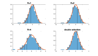
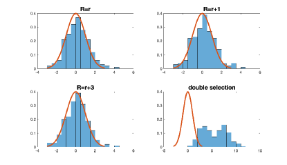
Figure 1: Histograms of the standardized estimates (4.12) over 200 replications, superimposed with the standard normal density. The panel of “double selection” corresponds to directly selecting among $\mathbf{x}_{t}$ (corresponding to $R=0$, no factor adjustment), while all other panels correspond to using diversified factor (DP) estimators with $R$ number of working factors. Top four figures correspond to $r=0$ and bottom four figures correspond to $r=2$. When $R\geq r$, (4.12) holds, whereas when $R<r$, (4.12) is violated. Figure source: Fan and Liao (2020).

Figure 1, taken from Fan and Liao (2020), plots the histograms of the t-statistics based on estimated $\boldsymbol{\beta}$ over 200 simulations, superimposed with the standard normal density, where $R$ diversified projections are used to estimate factors in step 1. Here the weights are the initial transformations ($t=0$) so that the $i^{th}$ row of $\mathbf{W}$ is $(x_{it},x_{it}^{2},\cdots,x_{it}^{R})$ at $t=0$. The “double selection” is the algorithm used in Belloni et al. (2014) that directly selecting among $\mathbf{x}_{t}$, corresponding to the case $R=0$. The factor-augmented algorithm works well even if $r=0$; but when $r\geq 1$ factors are present, “double selection” leads to severely biased estimations.

Therefore as a practical guidance, we recommend that one should always run factor-augmented post-selection inference, with $R\geq 1$, to guard against confounding factors among the control variables.

4.3 Factor-adjusted robust multiple testing

4.3.1 False discovery rate control

Controlling the false discovery proportion (FDP) in large-scale hypothesis testing based on strongly dependent tests has been an important problem in many scientific discoveries across disciplines. See Fan et al. (2019a) and references therein, and Barras et al. (2010); Harvey et al. (2015); Harvey and Liu (2018); Giglio et al. (2020) for applications in empirical asset pricing.

Suppose we observe realizations of a random vector $\{\mathbf{y}_{t}=(y_{1t},\cdots,y_{Nt})^{\prime}\}_{t=1}^{T}$. Let $\boldsymbol{\alpha}=(\alpha_{1},\cdots,\alpha_{N})^{\prime}$ denote its mean vector. We are interested in testing individual hypotheses:

$$H_{0}^{i}:\alpha_{i}=0,\quad i=1,\cdots,N.$$

Let $p_{i}$ denote the $p$-value for testing $H_{0}^{i}$ based on a test statistic such as $t$-test, which rejects if $p_{i}<x$ given some critical value $x$. Define the number of false discoveries (rejections) and the total number of rejections as follows:

$$\mathcal{F}(x) = \sum_{i=1}^{N}1\{i:p_{i}<x\text{ and $H_{0}^{i}$ is true}\},\qquad\mathcal{V}(x)=\sum_{i=1}^{N}1\{i:p_{i}<x\}.$$

In large-scale multiple testing problems, researchers often aim to control the false discovery proportion (FDP) and the false discovery rate (FDR) defined by

$$\text{FDP}(x)=\frac{\mathcal{F}(x)}{\max\{\mathcal{V}(x),1\}},\quad\text{FDR}(x)=\mathbb{E}\{\text{FDP}(x)\}.$$

The goal is to find the critical value $x$ so that FDR$(x)\leq\tau$ for a desired level $\tau$ (e.g., 0.10) or more relevantly FDP$(x)\leq\tau$ with high confidence. While $\mathcal{V}(x)$ is known, $\mathcal{F}(x)$ is not in practice. A general principle of finding $x$ proceeds as the following two steps.

Algorithm 4.3.

General principle for FDP/FDR control.

Step 1.

Find $\bar{\mathcal{F}}(x)$ such that either it upper bounds $\mathcal{F}(x)$ for all $x\in(0,1)$, or it estimates $\mathcal{F}(x)$ uniformly well.

Step 2.

Set the critical value to $x^{*}=\sup\{x\in(0,1):\bar{\mathcal{F}}(x)\leq\tau\max\{\mathcal{V}(x),1\}\}$.

One of the most popular procedures, proposed by Benjamini and Hochberg (1995), proceeds as follows. Denote $p_{(1)}\leq\cdots\leq p_{(N)}$ as the sorted p-values for the individual tests. Then the critical value is set to

$$x^{*}=\max\{p_{(i)}:p_{(i)}\leq\tau i/N\}.$$

This method fits into Algorithm 4.3 with $\bar{\mathcal{F}}(x)=Nx$, which is an asymptotic upper bound for $\mathcal{F}(x)$ when the individual p-values are independent. One of the limitations of this upper bound is that it is too conservative if the number of true negatives is small compared to $N$. More fundamentally, it requires the test statistics be weakly dependent, a topic we shall discuss in more detail next. Other methods, such as Storey (2002); Fan et al. (2012), etc., aim to directly estimate $\mathcal{F}(x)$ in step 1 in the presence of strong dependence among test statistics, and are also adaptive to the unknown number of true negatives.

In addition, instead of Algorithm 4.3, Romano and Wolf (2007); Romano et al. (2008) provided alternative procedures for FDR control.

4.3.2 Removing dependence by factor adjustments

The key to the success of FDR control is that the individual test statistic should be either weakly dependent or independent. This makes the FDR and FDP approximately the same and easier to control. On the other hand, suppose the cross-sectional dependence of $\mathbf{y}_{t}$ is generated from a latent factor model:

$$\mathbf{y}_{t}=\boldsymbol{\alpha}+\mathbf{B}\mathbf{f}_{t}+\mathbf{u}_{t},\quad\operatorname{\mathbb{E}}(u_{t}|\mathbf{f}_{t})=0,$$ (4.13)

where $\operatorname{\mathbb{E}}\mathbf{f}_{t}=0$, and $\boldsymbol{\alpha}$ is the mean vector. In empirical asset pricing, the model can be used to identify nonzero alphas out of a large number of assets, and has been studied to identify skilled mutual fund managers, e.g., Barras et al. (2010) and Harvey et al. (2015). The presence of latent factors, however, leads to strong dependence among the t-statistics based on the naive sample means of $\mathbf{y}_{t}$, which invalidates the weak dependence assumptions. As well documented in the literature, strong dependence creates fundamental challenges to multiple testing, including large standard errors among the estimated $\alpha_{i}$, unstable FDP’s, and conservativeness of the test procedure. Learning dependence $\mathbf{B}\mathbf{f}_{t}$ and removing it from the model (4.13) make the data not only weakly dependent but also less noisy (from $\mathbf{B}\mathbf{f}_{t}+\mathbf{u}_{t}$ to $\mathbf{u}_{t}$). This is the basic idea in factor-adjusted robust multiple tests (FarmTest) by using factor-adjusted data $\{\mathbf{y}_{t}-\widehat{\mathbf{B}}\widehat{\mathbf{f}_{t}}\}_{t=1}^{T}$; see (4.13). Furthermore, Fan et al. (2019a) makes adjustments so that it is also robust to heavy tailed data.

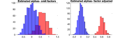
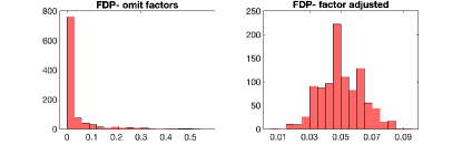
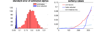
Figure 2: Comparison between the sample mean (omit factors) and the factor-adjusted method, with $T=200$ and $N=1000$. The upper panels plot the histograms of estimated individual alphas from a single simulation; the middle panels plot the individual FDP’s over 1000 simulations. The bottom left panel plots the cross-sectional histograms of standard errors of the estimated alphas over 1000 simulations. The bottom right panel plots the sorted p-values from a single simulation. The B-H procedure rejects all the hypotheses if $p_{(i)}$ is below the B-H threshold line $f(i):=\tau i/N$.

To illustrate consequences of omitting adjusting latent factors as well as the effectiveness of the use of the factor-adjusted method (to be detailed below), let us consider a numerical example of a single factor model, where elements of $\mathbf{u}_{t}$, $\mathbf{f}_{t}$ and $\mathbf{B}_{t}$ are generated from the standard normal distribution. We take the true means to be $\alpha_{i}=0.6$ for $1\leq i\leq N/4$ and 0 otherwise, and compare two estimated $\alpha_{i}$: 1) the sample means of $\mathbf{y}_{t}$, without using factor adjustments; 2) the factor-adjusted estimator based on PCA. We apply the method of Benjamini and Hochberg (1995) for multiple testing, setting $\tau=0.05$.

The top panels of Figure 2 plot the histograms, from a single simulation, of the estimators for $\alpha_{i}$, corresponding to those that satisfy the null hypotheses $\alpha_{i}=0$ and those that satisfy the alternatives $\alpha_{i}=0.6$. Clearly, there is a large overlap (on the upper left panel) between sample means from the null and alternative, making tests based on sample means difficult to distinguish the alternatives from the nulls. In contrast, the PCA-based estimator can easily separate the nulls and alternatives, as shown on the upper right panel in Figure 2.

The middle two panels of Figure 2 plot the histograms of the true FDP over 1000 simulations based on the two estimators. It is evident that the distribution of the FDP corresponding to the factor-adjusted estimator concentrates around the nominal level. In contrast, the one based on the sample mean has a noticeable long tail as well as a larger mean and variance, which demonstrate the challenge to control FPD in presence of common factors, as explained above.

Finally, omitting confounding factors would lead to larger standard errors and conservative inference. The bottom two panels in Figure 2 plot the standard errors of individual estimated alphas and the sorted p values for the two estimation methods. The sample-mean estimator has much fewer sorted p-values below the B-H threshold line (i.e., fewer rejections), compared to the factor-adjusted estimator.

Hence it is recommended to estimate and remove the latent factors before applying standard FDR control algorithms.

4.3.3 Identifying skilled hedge funds

Giglio et al. (2020) studied the problem of identifying hedge funds that are able to produce positive alphas (i.e., have “skill”), among thousands of existing funds. They considered a linear pricing model, where hedge fund returns are:

$$y_{it}=\alpha_{i}+\mathbf{b}_{i}^{\prime}\boldsymbol{\lambda}+\mathbf{b}_{i}^{\prime}(\mathbf{f}_{t}-\mathbb{E}\mathbf{f}_{t})+u_{it}.$$

In the model $\mathbf{f}_{t}$ contains both observable and latent factors. The model allows nontradable observable factors and $\boldsymbol{\lambda}$ is the vector of factor risk premia.

At a broad level, their methodology proceeds as the Fama-MacBeth regression integrated with the PCA to extract latent factors:

Algorithm 4.4.

Estimating alphas in the presence of latent and nontradable factors.

Step 1.

Run fund-by-fund time series regressions to estimate fund exposures (betas) to observable factors.

Step 2.

Apply PCA to the residuals to recover the latent factors and betas.

Step 3.

Implement cross-sectional regressions like Fama-MacBeth to estimate the risk premia of the factors (including both observable and latent factors) and the alphas.

Because of many negative alphas from unskilled hund managers, the multiple testing problem should be properly formulated as one-sided hypotheses:

$$H_{0}^{i}:\alpha_{i}\leq 0,\quad i=1,\cdots,N.$$

Hence rejecting $H_{0}^{i}$ indicates skilled fund manger $i$. On the other hand, the existence of potentially a very large number of negative alphas gives rise to the issue of power loss, only to add noises to the model. The loss of power associated with testing inequalities is well known as the problem of “deep in the null”, and is often seen in the econometric literature. To address this issue, Giglio et al. (2020) proposed to first screen off very bad funds, identified as:

$$\mathcal{I}=\{i\leq N,\widehat{\alpha}_{i}/\text{se}(\widehat{\alpha}_{i})<-c_{NT}\}$$

where $c_{NT}>0$ is a slowly growing sequence to ensure sure screening (Fan and Lv, 2008): $P(\mathcal{I}\subseteq\mathcal{H}_{0})\to 1$. They recommended to apply FDR control algorithms on funds outside $\mathcal{I}$. Therefore, there are two ingredients that are recommended for identifying skilled fund managers via multiple testing: (1) adjust the effect of latent factors, and (2) remove the estimated alphas that are deep in the null. Both are playing essential roles of gaining good testing power.

4.4 Instrumental variable regression

The issue of endogeneity is often encountered in real data applications. Consider the following instrumental variable (IV) regression model

$$y_{t}=\mathbf{w}_{t}^{\prime}\boldsymbol{\beta}^{0}+\varepsilon_{t}=\mathbf{w}_{1t}^{\prime}\boldsymbol{\beta}_{1}+\mathbf{w}_{2t}^{\prime}\boldsymbol{\beta}_{2}+\varepsilon_{t},$$

where $\mathbf{w}_{1t}$ is a $k_{1}$-dimensional vector of exogenous regressors and $\mathbf{w}_{2t}$ is a $k_{2}$-dimensional vector of endogenous regressors. Meanwhile, we have an $N$-dimensional IV $\mathbf{x}_{t}$ which admit a factor structure:

$$\mathbf{x}_{t}=\mathbf{B}\mathbf{f}_{t}+\mathbf{u}_{t}.$$

Below we introduce four estimators for $\boldsymbol{\beta}^{0}$, which differ on their choices of the instruments.

Use $\mathbf{f}_{t}$ as the instruments. Project $\mathbf{w}_{2t}$ on $\mathbf{f}_{t}$:

$$\mathbf{w}_{2t}=\boldsymbol{\phi}^{\prime}\mathbf{f}_{t}+\mathbf{v}_{t},\quad\mathbb{E}(\mathbf{v}_{t}|\mathbf{f}_{t})=0$$

where $\boldsymbol{\phi}$ is a $k_{2}\times r$ matrix. We need $r\geq k_{2}$ for identification. Let $\mathbf{z}_{t}=(\mathbf{w}_{1t}^{\prime},\mathbf{f}_{t}^{\prime})^{\prime}$ be the set of instruments. As $\mathbf{f}_{t}$ is unobservable, we replace it with some factor estimator and apply the two stage least squares estimator $\widehat{}\boldsymbol{\beta}_{\mathbf{f}}$ with the feasible instruments.

Bai and Ng (2010) studied this estimator, and showed that the estimation errors of $\widehat{}\boldsymbol{\beta}_{\mathbf{f}}$ associated with the generated instruments (factor estimations) have no effect on the limiting variance. When $\mathbf{u}_{t}$ and $\varepsilon_{t}$ are uncorrelated, this only requires $(N,T)\to\infty$ regardless of the relative growth rates. When some weak correlations are present but $\|\mathbb{E}\varepsilon_{t}\mathbf{u}_{t}\|_{1}=O(1)$, we would require $\sqrt{T}=o(N)$ to offset the effect of estimating factors.

Use $\mathbf{x}_{t}$ as the instruments. Project $\mathbf{w}_{2t}$ on $\mathbf{x}_{t}$:

$$\mathbf{w}_{2t}=\boldsymbol{\theta}\mathbf{x}_{t}+\mathbf{e}_{t},$$ (4.14)

where $\boldsymbol{\theta}$ is a $k_{2}\times N$ coefficient matrix. This projection motivates the use of $\mathbf{x}_{t}$ directly as a set of high-dimensional IV. Suppose that $\varepsilon_{t}$ is an i.i.d process, then the two-stage least squares estimator is efficient, and is given by

$$\widehat{}\boldsymbol{\beta}_{\mathbf{x}}=\Big{(}\mathbf{W}^{\prime}\mathbf{X}\widehat{}\boldsymbol{\Sigma}_{x}^{-1}\mathbf{X}^{\prime}\mathbf{W}\Big{)}^{-1}\mathbf{W}^{\prime}\mathbf{X}\widehat{}\boldsymbol{\Sigma}_{x}^{-1}\mathbf{X}^{\prime}\mathbf{Y}$$

where $\mathbf{X}$ is $T\times N$ matrix of $\mathbf{x}_{t}$; $\mathbf{W}$ and $\mathbf{Y}$ are matrices of $\mathbf{w}_{t}$ and $y_{t}$. Note that $\widehat{}\boldsymbol{\Sigma}_{x}$ is the estimated covariance of $\mathbf{x}_{t}$, which can be constructed using factor-based covariance estimators as described in Section 3. It is interesting to compare the asymptotic behaviors of $\widehat{}\boldsymbol{\beta}_{\mathbf{f}}$ with $\widehat{}\boldsymbol{\beta}_{\mathbf{x}}$. Bai and Ng (2010) showed when $\mathbf{u}_{t}$ and $\mathbf{w}_{t}$ are uncorrelated, they have the same asymptotic variance, but $\widehat{}\boldsymbol{\beta}_{\mathbf{x}}$ has a $O(\frac{N}{T})$ bias term. So $\widehat{}\boldsymbol{\beta}_{\mathbf{x}}$ is consistent only if $N=o(T)$.

Use selected $\mathbf{x}_{t}$ as the instruments. We still consider the projection (4.14), but assume that rows of $\boldsymbol{\theta}$ are sparse vectors so that we can apply penalized regression to select among the components of $\mathbf{x}_{t}$:

$$\widehat{}\boldsymbol{\theta}_{j}=\arg\min_{\boldsymbol{\theta}_{j}\in\mathbb{R}^{N}}\frac{1}{T}\sum_{t=1}^{T}(w_{2t,j}-\mathbf{x}_{t}^{\prime}\boldsymbol{\theta}_{j})^{2}+P_{\tau}(\boldsymbol{\theta}_{j}),\quad j\leq\dim(\mathbf{w}_{2t})$$ (4.15)

where $P_{\tau}(\boldsymbol{\theta}_{j})$ is a sparse-induced penalty with tuning $\tau$. Let $\mathbf{x}_{t,\text{selec}}$ be the vector of selected components corresponding to nonzero components of $\{\widehat{}\boldsymbol{\theta}_{j}:j\leq\dim(\mathbf{w}_{2t})\}$. Belloni et al. (2012) used $(\mathbf{w}_{1t},\mathbf{x}_{t,\text{selec}})$ as the instruments to compute $\widehat{}\boldsymbol{\beta}_{\mathbf{x},\text{selec}}$, the two stage least squares estimator. This method however, would not work well in the presence of common factors. The strong dependence in $\mathbf{x}_{t}$ invalidates the variable selection procedure (4.15).

Use $\mathbf{f}_{t}$ and selected $\mathbf{u}_{t}$ as the instruments. We are not aware of any applications of this method in the IV literature, but it is still well motivated. Substitute the factor structure to (4.14), we obtain

$$\mathbf{w}_{2t}=\boldsymbol{\delta}\mathbf{f}_{t}+\boldsymbol{\theta}\mathbf{u}_{t}+\mathbf{e}_{t}$$

where $\boldsymbol{\delta}=\boldsymbol{\theta}\mathbf{B}$. Hence we can carry out variable selections among $\mathbf{u}_{t}$:

$$(\widehat{}\boldsymbol{\delta}_{j},\widehat{}\boldsymbol{\theta}_{j})=\arg\min_{\boldsymbol{\delta}_{j}\in\mathbb{R}^{r},\boldsymbol{\theta}\in\mathbb{R}^{N}}\frac{1}{T}\sum_{t=1}^{T}(w_{2t,j}-\boldsymbol{\delta}_{j}^{\prime}\widehat{}\mathbf{f}_{t}-\widehat{}\mathbf{u}_{t}^{\prime}\boldsymbol{\theta}_{j})^{2}+P_{\tau}(\boldsymbol{\theta}_{j}),\quad j\leq\dim(\mathbf{w}_{2t}).$$

Let $\widehat{}\mathbf{u}_{t,\text{selec}}$ be the vector of selected components corresponding to nonzero components of $\{\widehat{}\boldsymbol{\theta}_{j}:j\leq\dim(\mathbf{w}_{2t})\}$. We then use $(\mathbf{w}_{1t},\widehat{}\mathbf{f}_{t},\widehat{}\mathbf{u}_{t,\text{selec}})$ as the instruments to compute $\widehat{}\boldsymbol{\beta}_{\mathbf{f},\mathbf{u}}$, the two stage least squares estimator. This method is expected to work well because it marginalizes out the strong factors in $\mathbf{x}_{t}$, leaving remaining components $\mathbf{u}_{t}$ being weakly dependent.

Let us conduct a simple simulation to study the finite sample behaviors of the aforementioned four estimators. We consider a model $y_{t}=\mathbf{w}_{2t}^{\prime}\boldsymbol{\beta}^{0}+\varepsilon_{t}$, with a single endogenous regressor $\mathbf{w}_{2t}$ generated from (4.14) with $\mathbf{e}_{t}=\varepsilon_{t}/2$. Here $\boldsymbol{\theta}=(2,1,-1,0...,0)$ and $\mathbf{x}_{t}$ admits a two-factor structure. Variables $(\varepsilon_{t},\mathbf{f}_{t},\mathbf{B},\mathbf{u}_{t})$ are independent standard normal. Finally, variable selections are based on lasso with the oracle tuning parameter that controls the score of the least squares function. For instance, for problem (4.15) we set $P_{\tau}(\boldsymbol{\theta})=\tau\|\boldsymbol{\theta}\|_{1}$ with $\tau=2.2\|\frac{1}{T}\sum_{t}\mathbf{x}_{t}\mathbf{e}_{t}\|_{\infty}$.

Table 1: Comparison among four IV methods

$N$	$T$	Bias				Standard deviation
		$\widehat{}\boldsymbol{\beta}_{\mathbf{f}}$	$\widehat{}\boldsymbol{\beta}_{\mathbf{x}}$	$\widehat{}\boldsymbol{\beta}_{\mathbf{x},\text{selec}}$	$\widehat{}\boldsymbol{\beta}_{\mathbf{f},\mathbf{u}}$	$\widehat{}\boldsymbol{\beta}_{\mathbf{f}}$	$\widehat{}\boldsymbol{\beta}_{\mathbf{x}}$	$\widehat{}\boldsymbol{\beta}_{\mathbf{x},\text{selec}}$	$\widehat{}\boldsymbol{\beta}_{\mathbf{f},\mathbf{u}}$
50	100	0.004	-0.993	0.003	0.008	0.215	0.001	0.061	0.058
200	100	0.008	-0.996	0.007	0.009	0.143	8e-4	0.056	0.054

Reported is based on 1000 replications. $\widehat{}\boldsymbol{\beta}_{\mathbf{f}}$ uses $\widehat{}\mathbf{f}_{t}$ as IV; $\widehat{}\boldsymbol{\beta}_{\mathbf{x}}$ uses $\mathbf{x}_{t}$ as IV; $\widehat{}\boldsymbol{\beta}_{\mathbf{x},\text{selec}}$ selects $\mathbf{x}_{t}$ as IV using lasso; $\widehat{}\boldsymbol{\beta}_{\mathbf{f},\mathbf{u}}$ uses $(\widehat{}\mathbf{f}_{t},\widehat{}\mathbf{u}_{t,\text{selec}})$ as IV, where $\widehat{}\mathbf{u}_{t}$ are selected using lasso.

Table 1 reports the bias and standard deviation of each estimator calculated from 1000 replications. First, using only estimated factors as the instruments ($\widehat{}\boldsymbol{\beta}_{\mathbf{f}}$) leads to the largest standard error. This is not surprising because it excludes the relevant information from $\mathbf{u}_{t}$ while the latter is correlated with $\mathbf{w}_{2t}$, so this method is less efficient. Secondly, using $\mathbf{x}_{t}$ as instruments without variable selection ($\widehat{}\boldsymbol{\beta}_{\mathbf{x}}$) has the smallest standard deviation, but is severely biased. Finally, the two instrumental selection based estimators ($\widehat{}\boldsymbol{\beta}_{\mathbf{x},\text{selec}}$ and $\widehat{}\boldsymbol{\beta}_{\mathbf{f},\mathbf{u}}$) perform favorably and similarly. But $\widehat{}\boldsymbol{\beta}_{\mathbf{x},\text{selec}}$ is not as stable, as it occasionally selects none of the instruments in our numerical experiments.

4.5 Boosting

Consider the following factor-augmented regression

$$y_{t+h}=c+\boldsymbol{\alpha}(\mathbf{L})^{\prime}\mathbf{w}_{t}+\boldsymbol{\gamma}(\mathbf{L})y_{t}+\boldsymbol{\beta}(\mathbf{L})^{\prime}\mathbf{f}_{t}+\varepsilon_{t+h}.$$ (4.16)

where $\boldsymbol{\alpha}(\mathbf{L})=\boldsymbol{\alpha}_{0}+\boldsymbol{\alpha}_{1}\mathbf{L}+\dots+\boldsymbol{\alpha}_{p}\mathbf{L}^{p}$, $\boldsymbol{\gamma}(\mathbf{L})=\boldsymbol{\gamma}_{0}+\boldsymbol{\gamma}_{1}\mathbf{L}+\dots+\boldsymbol{\gamma}_{q}\mathbf{L}^{q}$ and $\boldsymbol{\beta}(\mathbf{L})=\boldsymbol{\beta}_{0}+\boldsymbol{\beta}_{1}\mathbf{L}+\dots+\boldsymbol{\beta}_{l}\mathbf{L}^{l}$, all are lag operator polynomials. Suppose that $\mathbf{w}_{t}$ is a $k$-dimensional vector and $\mathbf{f}_{t}$ is an $r$-dimensional vector. The above predictive regression has $n=1+(p+1)k+(q+1)+(l+1)r$ parameters. It is likely that partial parameters are zero. So model selection devices can be conducted to choose a parsimonious model. Here we briefly describe a model selection method, known as boosting, which was proposed to use by Bai and Ng (2009) in this context.

Boosting is an ensemble meta-algorithm, which sequentially finds a “committee” of base learners and then makes a collective decisions by using a weighted linear combination of all base learners. The first successful and popular boosting algorithm is AdaBoost (Freund and Schapire, 1997). Friedman (2001) proposes a generic functional gradient descent (FGD) algorithm, which views the boosting as a method for function estimation. If the squared loss function is specified, the FGD algorithm reduces to the $L_{2}$-Boosting, which is studied in Friedman (2001) and Bühlmann and Yu (2003). Suppose that $(y_{t},\mathbf{z}_{t})_{t=1}^{T}$ are the observed target and predictive regressors over the sample period. The $L_{2}$-Boosting algorithm for estimating the conditional mean $\mathbb{E}(y_{t}|\mathbf{z}_{t})$ is given as follows.

Algorithm 4.5.

$L_{2}$-Boosting algorithm

Step 1

Initialize $\widehat{f}^{[0]}(\cdot)$ an offset value. The default value is $\widehat{f}^{[0]}(\cdot)\equiv\bar{y}$. Set $m=0$.

Step 2

Increase $m$ by 1. Compute the residuals $e_{t}=y_{t}-\widehat{f}^{[m-1]}(\mathbf{z}_{t})$ for $t=1,2,\dots,T$.

Step 3

Fit the residual vector $e_{1},\dots,e_{T}$ to $\mathbf{z}_{1},\dots,\mathbf{z}_{T}$ by the real-valued base procedure (e.g., regression):

$$(\mathbf{z}_{t},e_{t})_{t=1}^{T}\xlongrightarrow{base~{}procedure}\widehat{g}^{[m]}(\cdot).$$

Step 4

Update $\widehat{f}^{[m]}(\cdot)=\widehat{f}^{[m-1]}(\cdot)+\nu\cdot\widehat{g}^{[m]}(\cdot)$, where $0<\nu\leq 1$ is a step-length factor.

Step 5

Iterate steps 2 to 4 until $m=m_{\mathrm{stop}}$ for some stopping iteration $m_{\mathrm{stop}}$.

One can apply the above $L_{2}$-Boosting to the factor-augmented predictive regression (4.16). As seen in Algorithm 4.5, one needs to specify the base procedure in step 3. Bai and Ng (2009) suggest two methods depending on the way to deal with lags, which leads to the component-wise $L_{2}$-Boosting and block-wise $L_{2}$-Boosting. In component-wise $L_{2}$-Boosting, one treats each lag of each variable as an independent predictor and the base procedure is a simple linear regression. Therefore, step 3 is given as follows.

Algorithm 4.6.

Component-wise $L_{2}$-Boosting

Step 3.1

Let $\mathbf{z}_{t,j}$ denote a typical regressor in the regressors pool with $j=1,2,\dots,n$. Regress the current residual $e_{t}$ (the residual in the $m$-th repetition) on each $\mathbf{z}_{t,j}$ to obtain the coefficient $\widehat{}\mathbf{b}_{j}$. Compute the sum of squared residuals, denoted by SSR($j$).

Step 3.2

Determine $j_{m}$ by

$$j_{m}=\underset{1\leq j\leq n}{\mathrm{argmax}}~{}\mathrm{SSR}(j).$$

Step 3.3

$\widehat{g}^{[m]}(\mathbf{x}_{t})=\mathbf{z}_{t,j_{m}}\widehat{}\mathbf{b}_{j_{m}}$ if $\mathbf{x}_{t}=\mathbf{z}_{t,j_{m}}$, and 0 otherwise.

Another way is to only differentiate the predictors in the current period and treat the predictor and its multiple lags as a block. This gives rise to the block-wise $L_{2}$-Boosting. The base procedure now is a multivariate regression with the regressors being one predictor and its lags. See Bai and Ng (2009) for details.

4.6 Threshold regression with mixed integer optimization

Threshold regressions have been used in economic applications to capture potential structural changes on regression coefficients. The early literature models the threshold effect using some observable scalar variable $q_{t}$ as in:

$$y_{t}=\mathbf{w}_{t}^{\prime}\boldsymbol{\beta}+\mathbf{w}_{t}^{\prime}\boldsymbol{\delta}1\{q_{t}>\gamma\}+\varepsilon_{t},$$

where $\mathbf{w}_{t}$ and $q_{t}$ are adapted to the filtration $\mathcal{F}_{t-1}$; $(\boldsymbol{\beta},\boldsymbol{\delta},\gamma)$ is a vector of unknown parameters, and $\varepsilon_{t}$ satisfies the conditional mean restriction. Hence when $q_{t}>\gamma$, the regression function becomes $\mathbf{w}_{t}^{\prime}(\boldsymbol{\beta}+\boldsymbol{\delta})$; when $q_{t}\leq\gamma$, it reduces to $\mathbf{w}_{t}^{\prime}\boldsymbol{\beta}$ (Chan, 1993; Hansen, 2000). In practice, it might be controversial to choose which observed variable plays the role of $q_{t}$. For example, if the two different regimes represent the status of two environments of the population, arguably it is difficult to assume that the change of the environment is governed by just a single variable.

Seo and Linton (2007) and Lee et al. (2020) extended the model to multivariate threshold:

$$y_{t}=\mathbf{w}_{t}^{\prime}\boldsymbol{\beta}+\mathbf{w}_{t}^{\prime}\boldsymbol{\delta}1\{\boldsymbol{\gamma}^{\prime}\mathbf{f}_{t}>0\}+\varepsilon_{t},$$

where $\mathbf{f}_{t}$ is a vector of “factors” and $\boldsymbol{\gamma}$ is the corresponding unknown coefficients. So the model introduces a regime change due to a single index of factors. Allowing multivariate thresholding is important, because it permits the structural change to be governed by a potentially much larger dataset: $\mathbf{x}_{t}=\mathbf{B}\mathbf{f}_{t}+\mathbf{u}_{t},$ where $\dim(\mathbf{x}_{t})=N\to\infty$. So $\mathbf{f}_{t}$ can be unobserved factors that can be learned from $\mathbf{x}_{t}.$ For the identification purpose, suppose $\frac{1}{T}\sum_{t}\mathbf{f}_{t}\mathbf{f}_{t}^{\prime}=\mathbf{I}$ and $\mathbf{B}^{\prime}\mathbf{B}$ is diagonal, then $\boldsymbol{\gamma}$ and $\mathbf{f}_{t}$ are separately identified. This gives rise to the factor-driven two-regime regression model.

A natural strategy to estimate the model is to rely on least squares:

$$\min_{\boldsymbol{\beta},\boldsymbol{\delta},\boldsymbol{\gamma}}\sum_{t=1}^{T}(y_{t}-\mathbf{w}_{t}^{\prime}\boldsymbol{\beta}-\mathbf{w}_{t}^{\prime}\boldsymbol{\delta}1\{\boldsymbol{\gamma}^{\prime}\widehat{}\mathbf{f}_{t}>0\})^{2},$$

where $\widehat{}\mathbf{f}_{t}$ is the plugged-in PC-estimator of factors. Because the least squares problem is neither convex nor smooth in $\boldsymbol{\gamma}$, the computational task is demanding. Lee et al. (2020) recommended using algorithms based on mixed integer optimization (MIO). Introduce integers $d_{t}:=1\{\boldsymbol{\gamma}^{\prime}\widehat{}\mathbf{f}_{t}>0\}\in\{0,1\}$. The goal is to introduce linear constraints with respect to variables of optimization. Suppose there are known upper and lower bounds for $\delta_{j}$: $L_{j}\leq\delta_{j}\leq U_{j}$, where $\delta_{j}$ denotes the $j$th element of $\boldsymbol{\delta}$. Define $M_{t}\equiv\max_{\boldsymbol{\gamma}\in\Gamma}|\boldsymbol{\gamma}^{\prime}\widehat{}\mathbf{f}_{t}|$, where $\Gamma$ is the parameter space for $\boldsymbol{\gamma}$. Then it can be verified that the least squares problem is numerically equivalent to the following constraint MIO problem:

$$\min_{\boldsymbol{\beta},\boldsymbol{\delta},\boldsymbol{\gamma},\mathbf{d},\boldsymbol{\ell}}\sum_{t=1}^{T}(y_{t}-\mathbf{w}_{t}^{\prime}{\boldsymbol{\beta}}-\mathbf{w}_{t}^{\prime}\boldsymbol{\ell}_{t})^{2}$$ (4.17)

subject to (for any $\epsilon>0$), for each $t=1,\ldots,T$ and each $j=1,\ldots,\dim(\mathbf{w}_{t})$,

$$\begin{split}&\boldsymbol{\gamma}\in\Gamma,\;d_{t}\in\{0,1\},\;L_{j}\leq\delta_{j}\leq U_{j},\\ &(d_{t}-1)(M_{t}+\epsilon)<\boldsymbol{\gamma}^{\prime}\widehat{}\mathbf{f}_{t}\leq d_{t}M_{t},\\ &d_{t}L_{j}\leq\ell_{j,t}\leq d_{t}U_{j},\\ &L_{j}(1-d_{t})\leq\delta_{j}-\ell_{j,t}\leq U_{j}(1-d_{t}).\end{split}$$ (4.18)

Then, we can apply modern MIO packages (e.g., Gurobi) to solve for the optimal $(\boldsymbol{\beta},\boldsymbol{\delta},\boldsymbol{\gamma})$.

Finally, Lee et al. (2020) also derived the asymptotic distribution of the estimated coefficients and proposed inferences based on bootstraps. Under the condition that $T=O(N)$, they showed that the effect estimating factors is negligible on the asymptotic distribution of the estimated $(\boldsymbol{\beta},\boldsymbol{\delta})$, but would affect both the rate of convergence and the limiting distribution of the estimated $\boldsymbol{\gamma}$.

4.7 Community detection

The stochastic block model has been a popular approach to modeling networks (see Abbe (2017) for a recent review). We observe a graph of $N$ nodes. Let $\mathbf{A}=(a_{ij})\in\mathbb{R}^{N\times N}$ be the adjancy matrix of edges so that $a_{ij}=1$ if nodes $i$ and $j$ are connected, and $a_{ij}=0$ otherwise. Suppose each node belongs to one of $r$ communities, and the community that node $i$ belongs to is denoted by an unknown $\pi_{i}\in\{1,\cdots,r\}$. In addition, elements of $\mathbf{A}$ are random variables. Then stochastic block model assumes that

$$P(a_{ij}=1|\pi_{i}=k,\pi_{j}=l)=w_{k,l},$$

where $w_{k,l}$ is an unknown probability. We observe the matrix $\mathbf{A}$ and aim to recover the membership $\pi_{i}$ and the probabilities $w_{k,l}$ for all $k,l=1,\cdots,r$.

Let $\mathbf{e}_{1},\cdots,\mathbf{e}_{r}$ denote the canonical basis in $\mathbb{R}^{r}$, and $\mathbf{b}_{i}=\mathbf{e}_{k}$ where $\theta_{i}=k$. Then, $\mathbf{b}_{i}$ indicates the community membership of node $i$, and the membership matrix is

$$\mathbf{B}=(\mathbf{b}_{1},\cdots,\mathbf{b}_{N})^{\prime},\quad N\times r,$$

whose rows represent nodes and columns represent communities. Let $\mathbf{W}$ denote the $r\times r$ matrix of $(w_{k,l})$ and let $\mathbf{L}:=\operatorname{\mathbb{E}}\mathbf{A}$. It can easily be seen that $\mathbf{L}=\mathbf{B}\mathbf{W}\mathbf{B}^{\prime}$ is a low-rank matrix, whose rank equals $r$, leading to the following low-rank decomposition:

$$\mathbf{A}=\mathbf{L}+\mathbf{S},\quad\mathbf{S}=\mathbf{A}-\operatorname{\mathbb{E}}\mathbf{A}.$$

Therefore, $\mathbf{A}$ has the familiar decomposition (2.4), with $\mathbf{L}$ being similar to the systematic risk and $\mathbf{B}$ as a low-rank loading matrix. Since the elements in $\mathbf{S}$ are independent with mean-zero (Wigner matrix), the operator norm $\|\mathbf{S}\|$ does not grow too fast, compared to that of $\mathbf{L}$. We can then apply PCA on $\mathbf{A}$ to estimate $\mathbf{B}$. Suppose $r$ is known, then the estimator $\widehat{}\mathbf{B}$ is defined as $\sqrt{N}$ times the eigenvectors of $\mathbf{A}$, corresponding to the first $r$ eigenvalues.

Theorem 2.1 can be applied to obtain a deviation bound for the estimated loading matrix. If there is a sequence $g_{N}\to\infty$ and constants $c_{1},\cdots,c_{r}>0$ such that the eigenvalues $\lambda_{i}(\mathbf{W}^{1/2}\mathbf{B}^{\prime}\mathbf{B}\mathbf{W}^{1/2})=c_{i}g_{N}(1+o_{P}(1))$ for all $i\leq r$, then there is an $r\times r$ matrix $\mathbf{H}$, so that

$$\|\widehat{}\mathbf{B}-\mathbf{B}\mathbf{H}\|_{\infty}=O_{P}(g_{N}^{-2}N\|\mathbf{S}\|+g_{N}^{-1}\sqrt{N\log N}).$$

Therefore, elements of a rotated $\mathbf{B}$ can be estimated uniformly well. Moreover, because each community has many nodes belong to, $\mathbf{B}\mathbf{H}$ has many identical rows, which makes the cluster analysis as a natural method for community detections. For instance, we can apply either the K-means cluster analysis, or the homogeneous pursuit of Ke et al. (2015) on the rows of $\widehat{}\mathbf{B}$ to consistently identify the communities.

4.8 Time varying models

So far we have been assuming that the factor loading and covariance matrices are time-invariant. Research on conditional factor models has also grown rapidly in recent years. Suppose

$$y_{it}=\mathbf{b}_{i,t}^{\prime}\mathbf{f}_{t}+u_{it}$$

where $\mathbf{b}_{i,t}$ is a time-varying vector of loadings. There have been several approaches to addressing the issues of time-varying loadings. In this section we briefly review three of the most commonly used ones: (1) time-varying characteristics, (2) time-smoothing and (3) continuous-time models.

4.8.1 Time-varying characteristics

The first approach models $\mathbf{b}_{i,t}$ using a function of observed characteristics $\mathbf{z}_{i,t-1}$:

$$\mathbf{b}_{i,t}=\mathbf{b}_{i}(\mathbf{z}_{i,t-1})$$

where $\mathbf{b}_{i}(\cdot)$ is either a linear function or an unknown nonparametric function of the characteristics. Therefore, the time-varyingness is mainly captured by the characteristics. An advantage of this approach, over the other two approaches to be reviewed below, is that if $\mathbf{z}_{i,t-1}$ is correctly specified and indeed can fully capture the degree of time-varyingness of the model, then $\mathbf{b}_{i,t}$ allows a large degree of varyingness, and potentially, structural breaks. On the other hand, the limitation of this approach is the potential misspecification of $\mathbf{z}_{i,t-1}$ and omitted variable problems. Above all, we refer to Gagliardini et al. (2019) for an excellent review on conditional factor models using this approach, and their applications in empirical asset pricing.

4.8.2 Time-smoothing

The second approach assumes that factor loadings change smoothly over time. Suppose $\mathbf{b}_{i}(\cdot)$ is an unknown smooth function, we assume

$$\mathbf{b}_{i,t}=\mathbf{b}_{i}\left(\frac{t}{T}\right),\quad\forall t\leq T.$$

Then locally, $\mathbf{b}_{i,t}\approx\mathbf{b}_{i,r}$ for all $t\approx r$. So in a local window $\mathcal{B}(r)$ of each fixed $r$, the model is approximately time invariant:

$$y_{it}\approx\mathbf{b}_{i,r}^{\prime}\mathbf{f}_{t}+u_{it},\quad t\in\mathcal{B}(r).$$

Motivated by this assumption, Ang and Kristensen (2012) and Ma et al. (2020) tested the market mean-variance efficiency assumption in the case of known factor case. In the unknown factor case, Su and Wang (2017) first applied local smoothing on $y_{i,t}$ then employed PCA on the smoothed data to estimate the factors and loadings. While this approach does not require the specification of time-varying characteristics, it restricts to the smooth varying scenario and thus rules out structural breaks. In addition, slow rates of convergence appear near boundaries (that is, the beginning and the end of observing periods).

4.8.3 High-frequency factor models

Consider a continuous-time factor model

$$d\mathbf{y}_{t}=\boldsymbol{\alpha}_{t}dt+\mathbf{B}_{t}d\mathbf{f}_{t}+d\mathbf{u}_{t}$$

where $\mathbf{y}_{t}$, $\mathbf{f}_{t},\mathbf{u}_{t}$ are vectors of asset prices, factors and idiosyncratic risks; $\boldsymbol{\alpha}_{t}$ is a drift term. The time-varying loading matrix $\mathbf{B}_{t}$ is an $N\times r$ matrix that is assumed to be continuous and locally bounded Itô semimartingale of the form:

$$\mathbf{B}_{t}=\mathbf{B}_{0}+\int_{0}^{t}\widetilde{}\boldsymbol{\alpha}_{s}ds+\int_{0}^{t}\boldsymbol{\sigma}_{s}d\mathbf{W}_{s},$$

where $\widetilde{}\boldsymbol{\alpha}_{s}$ and $\boldsymbol{\sigma}_{s}$ are optional processes and locally bounded; $\mathbf{W}_{s}$ is a Brownian motion. Roughly speaking, by the Burkholder-Davis-Grundy inequality (cf. chapter 2 of Jacod and Protter (2011)), $\mathbf{B}_{t}$ is also locally time-invariant, which is similar to the treatment of the time-smoothing approach. The major difference though, is that the use of high-frequency data has automatically “smoothed” the data. We refer to the following papers for recent developments on high-frequency factor models, among others: Aït-Sahalia and Xiu (2017); Chen et al. (2019a); Liao and Yang (2018); Li et al. (2019); Pelger (2019).

5 Unbalanced Panels

Missing data and unbalanced panels are not uncommon in economic and financial studies. Addressing the missing data issue in statistical modeling belongs to a larger category of problems, known as matrix completion. Low-rank matrix completion refers to the problem of recovering missing entries from low-rank matrices. It is particularly relevant to empirical asset pricing factor models, because many time series of returns have short histories or missing records. In this section we review several methods for matrix completions, which assume that the missing is at random, except for Cai et al. (2016); Bai and Ng (2019). Besides, the EM algorithm is also a classical approach to dealing with unbalanced panels. We refer to Stock and Watson (2002b); Su et al. (2019); Zhu et al. (2019) for detailed discussions on related issues.

5.1 Inverse probability weighting

Recall that the covariance matrix of $\mathbf{y}_{t}$, under the factor model (3.1), has the following decomposition, $\boldsymbol{\Sigma}_{y}=\mathbf{B}\operatorname{cov}(\mathbf{f}_{t})\mathbf{B}^{\prime}+\boldsymbol{\Sigma}_{u},$ where columns of $\mathbf{B}$ are approximately equal to the eigenvectors of $\boldsymbol{\Sigma}_{y}$ corresponding to the first $r$ eigenvalues. As such, let $\widehat{}\boldsymbol{\Sigma}_{y}$ be an input matrix, serving as an estimator for $\boldsymbol{\Sigma}_{y}$. Then as described in Section 2.2, we can estimate the space spanned by $\mathbf{B}$ using the leading eigenvectors of $\widehat{}\boldsymbol{\Sigma}_{y}$.

In the presence of missing data with exogenous missing, let $x_{it}=1\{y_{it}\text{ is observed}\}$ and we only observe $y_{it}x_{it}$ for all $(i,t)$, in which unobserved data is set to zero. Suppose for now $w_{i}:=P(x_{it}=1)$ is known. We can construct an unbiased estimator $\widehat{}\boldsymbol{\Sigma}_{y}=(\widehat{\sigma}_{ij})$ with

$$\widehat{\sigma}_{ij}:=\frac{1}{w_{i}w_{j}T}\sum_{t=1}^{T}y_{it}y_{jt}x_{it}x_{jt}.$$

In the matrix form, let $\mathbf{Y}$ and $\mathbf{X}$ be the $N\times T$ matrices of $y_{it}$ and $x_{it}$. So we only observe $\mathbf{Y}\circ\mathbf{X}$, where $\circ$ represents the element-wise matrix product, the Hadamard product. Also let $\mathbf{W}$ be the diagonal matrix with $w_{i}$ being its $i$ th diagonal entry. Then

$$\widehat{}\boldsymbol{\Sigma}_{y}=\frac{1}{T}\mathbf{Z}\mathbf{Z}^{\prime},\quad\mathbf{Z}:=\mathbf{W}^{-1}\mathbf{Y}\circ\mathbf{X}.$$

Therefore, columns of the loading matrix estimator $\widehat{}\mathbf{B}$ equal to $\sqrt{N}$ times the top right singular vectors of $\mathbf{Z}$. This method simply replaces the missing entries of $\mathbf{Y}$ by zero, and apply the inverse probability weighting (IPW) before applying PCA. The IPW has been popularly used in the causal inference literature (e.g., Imbens and Rubin (2015)). Here the same idea is applied to create an unbiased estimator for the covariance matrix.

In practice, we shall replace $w_{i}$ by its consistent estimators, such as $\widehat{w}_{i}:=\frac{1}{T}\sum_{t=1}^{T}x_{it}$. But in the case of homogeneous missing, that is, $w_{1}=\cdots=w_{N}$, the IPW is not needed, because $\mathbf{W}$ equals the identity matrix up to a constant, which does not affect the PCA on $\mathbf{Y}\circ\mathbf{X}$. In addition, factors can be further estimated using least squares by regressing $y_{it}x_{it}$ on the estimated loadings.

Theoretical properties were studied by Abbe et al. (2020); Su et al. (2019) under the assumption of homogenous missing. Su et al. (2019) used this estimator as their initial value for the EM algorithm. Xiong and Pelger (2019) allowed heterogenous missing and proved that the estimators are also asymptotically normal (they estimated $w_{i}w_{j}$ directly by $\frac{1}{T}\sum_{t=1}^{T}x_{it}x_{jt}$). We can also quickly derive the rate of convergence by applying Theorem 2.1. However, the IPW is the least efficient approach among all the methods to be discussed in this section. We shall verify this in a simulation study in Section 5.5.

5.2 Regularized matrix completion

Regularized matrix completion is a powerful technique to recover missing entries from low-rank matrices. This approach is also much faster than the EM algorithm in handling large panels. Due to these nice properties, it has also attracted much attention in the recent econometrics literature, e.g., Athey et al. (2018); Bai and Ng (2017); Moon and Weidner (2018); Giglio et al. (2020).

In the matrix form $\mathbf{Y}=\mathbf{M}+\mathbf{U}$, the goal is to recover the factor component $\mathbf{M}=\mathbf{B}\mathbf{F}^{\prime}$ when $\mathbf{Y}$ has missing elements. The nuclear-norm regularization is directly applicable:

$$\widehat{}\mathbf{M}:=\arg\min_{\mathbf{M}}\|(\mathbf{Y}-\mathbf{M})\circ\mathbf{X}\|_{F}^{2}+\lambda\|\mathbf{M}\|_{n}$$ (5.1)

with tuning parameter $\lambda$. The factors and loadings can be estimated by taking the singular vectors of $\widehat{}\mathbf{M}$. Negahban and Wainwright (2011) and Koltchinskii et al. (2011) derived the rate of convergence under the Frobenius norm. Under suitable conditions (e.g., missing at random, restricted strong convexity, sufficiently large noise) it can be proved that

$$\frac{1}{NT}\|\widehat{}\mathbf{M}-\mathbf{M}\|_{F}^{2}=O_{P}\left(\frac{1}{T}+\frac{1}{N}\right).$$

Chen et al. (2020b) certifies further that the convex optimization (5.1) is optimal for all noise levels under Frobenius norm, operator norm, and elementwise-infinity norm. The proof is based on a novel technical device that bridges the convex optimization with a nonconvex optimization problem. However, this estimator is not asymptotically normal due to the presence of shrinkage bias, so is not suitable for statistical inferences.

5.3 Debiased estimators

Several recent progress in this literature focuses on debiasing the regularized regression in order to have valid confidence intervals, e.g., Chen et al. (2019b); Xia and Yuan (2019); Chernozhukov et al. (2019). When the missing is homogeneous, $P(x_{it}=1)=p$ for all $(i,t)$, Chen et al. (2019b) proposed the following simple debiased estimator

$$\widehat{\mathbf{M}}^{d}=H_{R}(\widehat{\mathbf{M}}+\widehat{p}^{-1}(\mathbf{Y}-\widehat{\mathbf{M}})\circ\mathbf{X}),$$ (5.2)

where $H_{R}(\cdot)$ is the best rank $R$ approximation in (2.5), $\widehat{\mathbf{M}}$ is given by (5.1), $\widehat{p}$ is the sample proportion of missing data. The idea is very intuitive. Ignoring the weak-dependence between $\widehat{\mathbf{M}}$ and $\mathbf{X}$ and estimating error in $\widehat{p}$, we have

$$\operatorname{\mathbb{E}}(\widehat{\mathbf{M}}+\widehat{p}^{-1}(\mathbf{Y}-\widehat{\mathbf{M}})\circ\mathbf{X})\approx\operatorname{\mathbb{E}}\widehat{\mathbf{M}}+\operatorname{\mathbb{E}}(\mathbf{Y}-\widehat{\mathbf{M}})=\mathbf{M},$$

which is approximately unbiased. However, the estimator $\widehat{\mathbf{M}}+\widehat{p}^{-1}(\mathbf{Y}-\widehat{\mathbf{M}}\circ\mathbf{X})$ is no longer of rank $R$, which increases the variances. This leads to use the projection as in (5.2), which is asymptotically efficient in terms of both rate and pre-constant.

Alternatively, the debiasing can be achieved through the iterative least squares (Chernozhukov et al., 2019). Suppose the true number of factors, $r$, is known.

Algorithm 5.1.

Debias using iterative least squares.

Step 1.

Obtain $\widehat{}\mathbf{M}$ as in (5.1).

Step 2.

Let the columns of $\frac{1}{\sqrt{N}}\widehat{}\mathbf{B}$ be the left singular vectors of $\widehat{}\mathbf{M}$, corresponding to the first $r$ singular values.

Step 3.

Estimate the latent factors at time $t$ by $\widetilde{}\mathbf{f}_{t}:=\left(\sum_{i=1}^{N}\widehat{}\mathbf{b}_{i}\widehat{}\mathbf{b}_{i}^{\prime}x_{it}\right)^{-1}\sum_{i=1}^{N}\widehat{}\mathbf{b}_{i}y_{it}x_{it}$ and let $\widetilde{}\mathbf{F}=(\widetilde{}\mathbf{f}_{1},\cdots,\widetilde{}\mathbf{f}_{T})^{\prime}$.

Step 4.

Update loading estimates by $\widetilde{}\mathbf{B}=(\widetilde{}\mathbf{b}_{1},\cdots,\widetilde{}\mathbf{b}_{N})^{\prime}$, where

$$\widetilde{}\mathbf{b}_{i}:=\left(\sum_{t=1}^{T}\widetilde{}\mathbf{f}_{t}\widetilde{}\mathbf{f}_{t}^{\prime}x_{it}\right)^{-1}\sum_{t=1}^{T}\widetilde{}\mathbf{f}_{t}y_{it}x_{it}.$$

Step 5.

The asymptotically unbiased estimator for $\mathbf{M}$ is $\widetilde{}\mathbf{M}:=\widetilde{}\mathbf{B}\widetilde{}\mathbf{F}^{\prime}.$

A key technical argument is to ensure that the estimation error in $\widehat{}\mathbf{B}$ (step 2) has no impact on the factor estimator (step 3); this is achieved by Chen et al. (2019b) using an “auxiliary leave-one-out” argument.

When the missing probability $P(x_{it}=1)$ varies across $i$, there are two ways to revise the previous algorithm to achieve the asymptotic normality. One way is to replace (5.1) with a weighted regularization:

$$\min_{\mathbf{M}}\|(\widehat{}\mathbf{W}^{-1/2}\mathbf{Y}-\widehat{}\mathbf{W}^{-1/2}\mathbf{M})\circ\mathbf{X}\|_{F}^{2}+\lambda\|\mathbf{M}\|_{n},$$ (5.3)

where $\widehat{}\mathbf{W}$ is a diagonal matrix, whose $i$ th diagonal entry equals $\widehat{w}_{i}:=\frac{1}{T}\sum_{t=1}^{T}x_{it}$. This debiases the least squares part of the loss function, adopting the same idea of inverse probability weighting. The remaining steps of Algorithm 5.1 are the same. Then the same “auxiliary leave-one-out” technical argument of Chen et al. (2019b) still goes through. The other way is to apply “sample splitting”, which evenly split the columns of $\mathbf{Y}$ into two parts: on one part we run the penalized regression as in (5.1) and obtain $\widehat{}\mathbf{B}$, on the other part we run iterative least squares. Then exchange the two parts and re-do the estimations. The final estimator is taken as the average of the two. Suppose $u_{it}$ is serially independent, the sample splitting then artificially creates independences among various statistics from the splitting sample. See Chernozhukov et al. (2019) for detailed descriptions of this approach.

5.4 Block-rearrangements

In an attempt to handle endogenous missing, Bai and Ng (2019) proposed a block-rearrangement method. At the cost of this generality, they require that the data matrix $\mathbf{Y}$ should have a sufficiently large balanced sub-block after elementary rearrangements. See Cai et al. (2016); Fan and Kim (2019) for related ideas.

Specifically, a preliminary step of their estimation is to rearrange the data in a shape that all the factor loadings can be estimated in one sub-block and all the factors can be estimated in another sub-block. The following example is adapted from Bai and Ng (2019), which gives a good illustration on this manipulation: example of the $N\times T$ matrix for $y_{it}$:

$$\begin{bmatrix}\mathbf{y}_{11}&\mathbf{y}_{12}&\mathbf{y}_{13}&\mathbf{y}_{14}&\mathbf{y}_{15}\\ \mathbf{y}_{21}&\mathbf{y}_{22}^{*}&\mathbf{y}_{23}&\mathbf{y}_{24}&\mathbf{y}_{25}\\ \mathbf{y}_{31}&\mathbf{y}_{32}&\mathbf{y}_{33}&\mathbf{y}_{34}^{*}&\mathbf{y}_{35}\\ \mathbf{y}_{41}^{*}&\mathbf{y}_{42}&\mathbf{y}_{43}&\mathbf{y}_{44}&\mathbf{y}_{45}\\ \mathbf{y}_{51}&\mathbf{y}_{52}&\mathbf{y}_{53}&\mathbf{y}_{54}&\mathbf{y}_{55}\end{bmatrix}\Longrightarrow\begin{bmatrix}\mathbf{y}_{13}&\mathbf{y}_{15}&{\color[rgb]{0,0,1}\mathbf{y}_{11}}&{\color[rgb]{0,0,1}\mathbf{y}_{12}}&{\color[rgb]{0,0,1}\mathbf{y}_{14}}\\ \mathbf{y}_{53}&\mathbf{y}_{55}&{\color[rgb]{0,0,1}\mathbf{y}_{51}}&{\color[rgb]{0,0,1}\mathbf{y}_{52}}&{\color[rgb]{0,0,1}\mathbf{y}_{54}}\\ {\color[rgb]{1,0,0}\mathbf{y}_{23}}&{\color[rgb]{1,0,0}\mathbf{y}_{25}}&{\color[rgb]{0,1,1}\mathbf{y}_{21}}&{\color[rgb]{0,1,1}\mathbf{y}_{22}^{*}}&{\color[rgb]{0,1,1}\mathbf{y}_{24}}\\ {\color[rgb]{1,0,0}\mathbf{y}_{33}}&{\color[rgb]{1,0,0}\mathbf{y}_{35}}&{\color[rgb]{0,1,1}\mathbf{y}_{31}}&{\color[rgb]{0,1,1}\mathbf{y}_{32}}&{\color[rgb]{0,1,1}\mathbf{y}_{34}^{*}}\\ {\color[rgb]{1,0,0}\mathbf{y}_{43}}&{\color[rgb]{1,0,0}\mathbf{y}_{45}}&{\color[rgb]{0,1,1}\mathbf{y}_{41}^{*}}&{\color[rgb]{0,1,1}\mathbf{y}_{42}}&{\color[rgb]{0,1,1}\mathbf{y}_{44}}\end{bmatrix}.$$

The left matrix is the originally collected data and the right is the rearranged one. The symbols with asterisk denote the missing data. From the column perspective, the 1st, 2nd and 4th columns have missing values and therefore are rearranged as the last three columns in the right panel; from the row perspective, the 2nd, 3rd and 4th rows have missing values and therefore are rearranged as the last three rows in the right panel. Bai and Ng (2019) name the black block “bal”, name the black plus the red blocks “tall”, and name the black plus the blue block “wide”.

Consider the missing value $\mathbf{y}_{22}^{*}$. We want to replace it with its expected value $\mathbb{E}(\mathbf{y}_{22}^{*})=\mathbf{b}_{2}^{\prime}\mathbf{f}_{2}$. Note that $\mathbf{y}_{22}^{*}$ shares the same factor loadings $\mathbf{b}_{2}$ with data points $\mathbf{y}_{23}$ and $\mathbf{y}_{25}$ in the wide block; and shares the same factors $\mathbf{f}_{2}$ with data points $\mathbf{y}_{12}$ and $\mathbf{y}_{52}$ in the tall block. Meanwhile, $\mathbf{b}_{2}$ can be estimated using data in the“tall” block; $\mathbf{f}_{2}$ can be estimated using data in the “wide” block. As a result, one might expect to recover $\mathbb{E}(\mathbf{y}_{22}^{*})$ with these two estimators. However, we must take into account the rotational indeterminacy inherent with the factor models. For a generic missing value $\mathbf{y}_{it}$,

$$\widehat{}\mathbf{b}_{\mathrm{tall},i}=\mathbf{H}_{\mathrm{tall}}^{\prime}\mathbf{b}_{i}+o_{P}(1),\quad\widehat{}\mathbf{f}_{\mathrm{wide},t}=\mathbf{H}_{\mathrm{wide}}^{-1}\mathbf{f}_{t}+o_{P}(1).$$

Therefore

$$\mathbf{b}_{i}^{\prime}\mathbf{f}_{t}=\widehat{}\mathbf{b}_{\mathrm{tall},i}^{\prime}\mathbf{A}\widehat{}\mathbf{f}_{\mathrm{wide},t}+o_{P}(1),\quad\mathbf{A}:=\mathbf{H}_{\mathrm{tall}}^{-1}\mathbf{H}_{\mathrm{wide}}.$$

To estimate $\mathbf{A}$, by $\widehat{}\mathbf{f}_{\mathrm{wide},t}=\mathbf{H}_{\mathrm{wide}}^{-1}\mathbf{f}_{t}+o_{P}(1)$ and $\widehat{}\mathbf{f}_{\mathrm{tall},t}=\mathbf{H}_{\mathrm{tall}}^{-1}\mathbf{f}_{t}+o_{P}(1)$, we have

$$\widehat{}\mathbf{f}_{\mathrm{tall},t}=\mathbf{A}\widehat{}\mathbf{f}_{\mathrm{wide},t}+o_{P}(1).$$

So one can run the regression of $\widehat{}\mathbf{f}_{\mathrm{tall},t}$ on $\widehat{}\mathbf{f}_{\mathrm{wide},t}$ to consistently estimate $\mathbf{A}$. This leads to the following estimation procedure.

Algorithm 5.2.

Block-rearrangement algorithm

Step 1

Obtain estimators $(\widehat{}\mathbf{b}_{\mathrm{wide}},\widehat{}\mathbf{F}_{\mathrm{wide}})$ using the tall block of $\mathbf{Y}$.

Step 2

Obtain estimators $(\widehat{}\mathbf{b}_{\mathrm{tall}},\widehat{}\mathbf{F}_{\mathrm{tall}})$ using the wide block of $\mathbf{Y}$.

Step 3

Compute $\widehat{}\mathbf{C}_{\mathrm{miss}}=\widehat{}\mathbf{B}_{\mathrm{tall}}\mathbf{A}\widehat{}\mathbf{F}_{\mathrm{wide}}^{\prime}$ where $\mathbf{A}$ is obtained by regressing $\widehat{}\mathbf{f}_{\mathrm{tall},t}$ on $\widehat{}\mathbf{f}_{\mathrm{wide},t}$

Step 4

Output $\widetilde{}\mathbf{Y}$, where $\widetilde{y}_{it}=y_{it}$ if $y_{it}$ is observable; $\widetilde{y}_{it}=\widehat{c}_{\mathrm{miss},it}$ if $y_{it}$ is missing.

Once $\widetilde{}\mathbf{Y}$ is obtained, we apply the PCA again to the imputed data $\widetilde{}\mathbf{Y}$ to get more efficient estimates of $\mathbf{B}$ and $\mathbf{F}$. Suppose the size of the “tall” block is $N\times T_{0}$ and the size of the “wide” block is $N_{0}\times T$. So the size of the “bal” block is $N_{0}\times T_{0}$. The whole sample size (including missing data points) is $N\times T$. Bai and Ng require that

$$\max\{\sqrt{N},\sqrt{T}\}=o(N_{0}),\quad\text{ and }\quad\max\{\sqrt{N},\sqrt{T}\}=o(T_{0}).$$

An implication of the above condition is that the missing data points should not be too frequent in the sense that the balanced subblock is large enough. Though this condition rules out the case of random missing (e.g., missing occurs as outcomes of Bernoulli trials), it is not stringent given the nature of endogenous missing.

5.5 A simulation study

We conduct a simulation study to compare six matrix completion approaches, namely:

IPW. The inverse probability weighting.

ReUW. Unweighted regularization. The eigenvectors of the estimator (5.1).

ReW. Weighted regularization. The eigenvectors of the estimator (5.3).

ReDebias. The debiased regularized estimator from Algorithm 5.1.

EM. The EM algorithm.

We generate a two-factor model where loadings, factors and $u_{it}$ are independent standard normal. Under the homogeneous missing we generate $x_{it}\sim$ Bernoulli$(0.5)$; under the heterogeneous missing we generate $x_{it}|w_{i}\sim$ Bernoulli$(w_{i})$, and $w_{i}\sim$Uniform$[0.1,1]$. The three regularized methods require choosing $\lambda$, the tuning parameter. Write the penalized loss function to be $\|(\mathbf{W}^{-1/2}\mathbf{Y}-\mathbf{W}^{-1/2}\mathbf{M})\circ\mathbf{X}\|_{F}^{2}+\lambda\|\mathbf{M}\|_{n}$ where $\mathbf{W}$ is a diagonal weighting matrix. The theory requires that with a high probability, there is $c>0$,

$$(2+c)\|\mathbf{U}\circ(\mathbf{W}^{-1}\mathbf{X})\|<\lambda.$$

So we set $\lambda$ to be the 0.95 quantile of $2.2\|\mathbf{Z}\circ(\mathbf{W}^{-1}\mathbf{X})\|$ where $\mathbf{Z}$ is an $N\times T$ matrix of standard normal variables. In practice, one can also simulate $\mathbf{Z}$ using the estimated idiosyncratic covariance matrix.

Table 2: Comparison among five matrix completion methods

$N$	$T$	IPW	ReUW	ReW	ReDebias2	EM
		Homogeneous missing
100	200	0.176	0.116	0.114	0.109	0.109
200	100	0.252	0.171	0.169	0.161	0.161
		Heterogeneous missing
100	200	0.263	0.211	0.131	0.119	0.119
200	100	0.369	0.304	0.222	0.204	0.203

Reported is $\|\mathbf{P}_{\widehat{}\mathbf{B}}-\mathbf{P}_{\mathbf{B}}\|$ averaged over 100 replications.

We compare the performance of estimating the loading space, measured by $\mathbf{P}_{\mathbf{B}}=\mathbf{B}(\mathbf{B}^{\prime}\mathbf{B})^{-1}\mathbf{B}^{\prime}$. Table 2 reports $\|\mathbf{P}_{\widehat{}\mathbf{B}}-\mathbf{P}_{\mathbf{B}}\|$ averaged over 100 replications for each method. In all scenarios, the IPW performs the worst among all estimators. Under the homogeneous missing, all the other four methods perform similarly, but the difference is much more noticeable under the heterogeneous missing. The general ranking is that

$$\text{IPW}\prec\text{ReUW}\prec\text{ReW}\prec\text{ReDebias}\approx\text{EM}.$$

This ranking is as expected: IPW is the least efficient method among the five; ReUW uses the nuclear-norm regularized estimation that does not take into account the heterogeneous missing or debias; ReW accounts for the heterogeneous missing probabilities, and ReDebias further removes the regularization bias.

Finally, it is not surprising to see that ReDebias and EM perform similarly because both start with an initial low-rank estimator (ReDebias initializes from ReW while EM initializes from IPW), then proceed via iterative least squares. But we note that ReDebias operates much faster because it only iterates once, so is more attractive than EM in handling large scale problems. We also implemented the “early-stop-EM” (which only iterates twice), it performs only slightly better than IPW and is worse than all the other estimators. Therefore we conclude that the ReDebias is a recommended method for handling large scale low-rank matrix completion problems.

6 Conclusion

We have conducted a selective overview on the recent developments of the factor model and its application on statistical learning. We focus on the perspective of the low-rank structure of factor models, and particularly draws attentions to estimating the model from the low-rank recovery point of view. New estimation and inference methods, and matrix completion problems have been discussed.

Appendix A Technical details

A.1 Proof of Theorem 2.1

Proof.

(i) The proof is an exercise of applying the eigen-perturbation theorem. First, by the triangular inequality, for $a_{N}:=2\eta_{N}\|\mathbf{L}\|+\eta_{N}^{2}+3\|\mathbf{L}\|\|\mathbf{S}\|$,

$$\|\widehat{}\boldsymbol{\Sigma}\widehat{}\boldsymbol{\Sigma}^{\prime}-\mathbf{L}\mathbf{L}^{\prime}\|\leq\|\boldsymbol{\Sigma}\boldsymbol{\Sigma}^{\prime}-\widehat{}\boldsymbol{\Sigma}\widehat{}\boldsymbol{\Sigma}^{\prime}\|+\|\boldsymbol{\Sigma}\boldsymbol{\Sigma}^{\prime}-\mathbf{L}\mathbf{L}^{\prime}\|\leq O_{P}(a_{N}).$$

So by Weyl’s theorem (cited in Theorem A.2), $\max_{i\leq r+1}|\lambda_{i}^{2}(\widehat{}\boldsymbol{\Sigma})-\lambda^{2}_{i}(\mathbf{L})|\leq O_{P}(a_{N}).$

Also, $g_{N}^{2}:=\min_{2\leq i\leq r+1}|\lambda_{i-1}(\mathbf{L})-\lambda_{i}(\mathbf{L})|^{2}\gg a_{N}$ implies $\lambda_{r}^{2}(\mathbf{L})\gg a_{N}$ and

$$\min_{2\leq i\leq r+1}|\lambda_{i-1}^{2}(\mathbf{L})-\lambda^{2}_{i}(\mathbf{L})|\geq 2\lambda_{r}(\mathbf{L})\min_{2\leq i\leq r+1}|\lambda_{i-1}(\mathbf{L})-\lambda_{i}(\mathbf{L})|\gg a_{N}.$$

So with probability approaching one,

$$\max_{i\leq r}|\lambda_{i}(\widehat{}\boldsymbol{\Sigma})-\lambda_{i}(\mathbf{L})| \leq \frac{\max_{i\leq r}|\lambda_{i}^{2}(\widehat{}\boldsymbol{\Sigma})-\lambda^{2}_{i}(\mathbf{L})|}{\min_{i\leq r}\sqrt{2\lambda_{i}^{2}(\mathbf{L})-|\lambda_{i}^{2}(\widehat{}\boldsymbol{\Sigma})-\lambda^{2}_{i}(\mathbf{L})|}}=O_{P}\left(\frac{a_{N}}{\lambda_{r}(\mathbf{L})}\right).$$ (A.1)

$$\min_{i\leq r}|\lambda_{i-1}^{2}(\widehat{}\boldsymbol{\Sigma})-\lambda^{2}_{i}(\mathbf{L})| \geq \min_{2\leq i\leq r}|\lambda_{i-1}^{2}(\mathbf{L})-\lambda^{2}_{i}(\mathbf{L})|-|\lambda_{i-1}^{2}(\widehat{}\boldsymbol{\Sigma})-\lambda^{2}_{i-1}(\mathbf{L})|$$ (A.2)

$$\geq \frac{1}{2}\min_{2\leq i\leq r}|\lambda_{i-1}^{2}(\mathbf{L})-\lambda^{2}_{i}(\mathbf{L})|.$$ (A.3)

Similarly, for all $i\leq r-1$, $|\lambda^{2}_{i}(\mathbf{L})-\lambda^{2}_{i+1}(\widehat{}\boldsymbol{\Sigma})|\geq\frac{1}{2}\min_{2\leq i\leq r}|\lambda_{i-1}^{2}(\mathbf{L})-\lambda^{2}_{i}(\mathbf{L})|.$ Now for $i=r$, $\lambda_{r+1}^{2}(\widehat{}\boldsymbol{\Sigma})\leq\lambda^{2}_{r+1}(\mathbf{L})+O_{P}(a_{N})=O_{P}(a_{N})$. So $|\lambda^{2}_{r}(\mathbf{L})-\lambda^{2}_{r+1}(\widehat{}\boldsymbol{\Sigma})|\geq\frac{1}{2}\lambda^{2}_{r}(\mathbf{L})$. Hence by the sing-theta theorem (cited in Theorem A.2),

$$\max_{i\leq r}\|\widehat{}\boldsymbol{\xi}_{i}-\boldsymbol{\xi}_{i}\|=O_{P}\left(\frac{a_{N}}{g^{2}_{N}}\right).$$ (A.4)

The right singular vectors have the same bound. Then (A.1) (A.4) together imply

$$\|\widehat{}\mathbf{L}-\mathbf{L}\|=O_{P}\left(\frac{a_{N}\|\mathbf{L}\|}{g^{2}_{N}}\right).$$

Finally, we note that $\|\mathbf{L}\|=\sum_{i=2}^{r+1}\lambda_{i-1}(\mathbf{L})-\lambda_{i}(\mathbf{L})\leq rg_{N}$. So $a_{N}=o_{P}(g_{N}^{2})$ is satisfied as long as $\|\mathbf{S}\|+\eta_{N}=o_{P}(g_{N})$ and $a_{N}=O_{P}(g_{N}\eta_{N}+g_{N}\|S\|)$.

(ii) The element-wise bound is a corollary from the more general bound in Theorem A.3. Using the notation of Theorem A.3, under the assumptions that $\|\boldsymbol{\Sigma}\|_{\infty}=O_{P}(1)$, $s_{N}=O_{P}(\sqrt{N_{1}})$. Also, $m_{N}=O_{P}(\frac{1}{\sqrt{N}}+\frac{1}{\sqrt{N_{1}}})$, $\|\mathbf{L}\|_{\infty}=O_{P}(1)$, $N_{1}c_{N}=o_{P}(g_{N})$. Hence

$$b_{N}\leq\left(\frac{N_{1}}{\sqrt{N}}+\sqrt{N_{1}}\right)g_{N}^{-2}(\eta_{N}+\|\mathbf{S}\|)+\left(c_{N}\frac{N_{1}}{\sqrt{N}}+c_{N}\sqrt{N_{1}}+\|\mathbf{S}\boldsymbol{\zeta}_{d}\|_{\infty}\right)g_{N}^{-1}.$$

∎

A.2 Proof of Theorem 3.1

Proof.

Let $Q(\mathbf{L},\boldsymbol{\Sigma}_{u})$ denote the loss function. Note that

$$\|\mathbf{S}_{y}-\widehat{}\mathbf{L}-\widehat{}\boldsymbol{\Sigma}_{u}\|_{F}^{2} = \|\mathbf{S}_{y}-\boldsymbol{\Sigma}_{y}\|_{F}^{2}+\|\widehat{}\mathbf{L}+\widehat{}\boldsymbol{\Sigma}_{u}-\mathbf{L}-\boldsymbol{\Sigma}_{u}\|_{F}^{2}+M_{1}+M_{2}$$

$$M_{1} = 2\operatorname{tr}((\mathbf{S}_{y}-\boldsymbol{\Sigma}_{y})(\mathbf{L}-\widehat{}\mathbf{L})^{\prime})$$

$$M_{2} = 2\operatorname{tr}((\mathbf{S}_{y}-\boldsymbol{\Sigma}_{y})(\boldsymbol{\Sigma}_{u}-\widehat{}\boldsymbol{\Sigma}_{u})^{\prime}).$$

We now use two types of inequalities to bound $M_{1}$ and $M_{2}$. As for $M_{1}$, note that $\mathbf{L}$ is a low-rank matrix, we use the inequality $|\operatorname{tr}(\mathbf{A}\mathbf{B}^{\prime})|\leq\|\mathbf{A}\|\|\mathbf{B}\|_{n}$. We thus have

$$|M_{1}|\leq 2\|\mathbf{S}_{y}-\boldsymbol{\Sigma}_{y}\|\|\mathbf{L}-\widehat{}\mathbf{L}\|_{n}\leq 0.5\nu_{1}\|\mathbf{L}-\widehat{}\mathbf{L}\|_{n}.$$

As for $M_{2}$, note that $\boldsymbol{\Sigma}_{u}$ is a sparse matrix, we use the inequality $|\operatorname{tr}(\mathbf{A}\mathbf{B}^{\prime})|\leq\|\mathbf{A}\|_{\infty}\|\mathbf{B}\|_{1}$,

$$|M_{2}|\leq 2\|\mathbf{S}_{y}-\boldsymbol{\Sigma}_{y}\|_{\infty}\|\boldsymbol{\Sigma}_{u}-\widehat{}\boldsymbol{\Sigma}_{u}\|_{1}\leq 0.5\nu_{2}\|\boldsymbol{\Sigma}_{u}-\widehat{}\boldsymbol{\Sigma}_{u}\|_{1}.$$

From Lemma 2.3 of Recht et al. (2010), $\|\mathbf{L}+\mathcal{P}(\mathbf{A}_{1})\|_{n}=\|\mathbf{L}\|_{n}+\|\mathcal{P}(\mathbf{A}_{1})\|_{n}$ where $\mathbf{A}_{1}=\widehat{}\mathbf{L}-\mathbf{L}$. Also using the standard sparse argument, $\|\boldsymbol{\Sigma}_{u}+(\mathbf{A}_{2})_{J^{c}}\|_{1}=\|\boldsymbol{\Sigma}_{u}\|_{1}+\|(\mathbf{A}_{2})_{J^{c}}\|_{1}$ where $\mathbf{A}_{2}=\widehat{}\boldsymbol{\Sigma}_{u}-\boldsymbol{\Sigma}_{u}$. In addition, Lemma 1 of Negahban and Wainwright (2011) shows $0.5\text{rank}(\mathcal{M}(\mathbf{A}_{1}))\leq r:=\text{rank}(\mathbf{L})$. Hence

$$\|\widehat{}\mathbf{L}\|_{n} = \|\mathbf{L}+\mathcal{P}(\mathbf{A}_{1})+\mathcal{M}(\mathbf{A}_{1})\|_{n}\geq\|\mathbf{L}\|_{n}+\|\mathcal{P}(\mathbf{A}_{1})\|_{n}-\|\mathcal{M}(\mathbf{A}_{1})\|_{n}$$

$$\|\widehat{}\boldsymbol{\Sigma}_{u}\|_{1} = \|\boldsymbol{\Sigma}_{u}+(\mathbf{A}_{2})_{J^{c}}+(\mathbf{A}_{2})_{J}\|_{1}\geq\|\boldsymbol{\Sigma}_{u}\|_{1}+\|(\mathbf{A}_{2})_{J^{c}}\|_{1}-\|(\mathbf{A}_{2})_{J}\|_{1},$$

$$\|\mathcal{M}(\mathbf{A}_{1})\|_{n} \leq \|\mathcal{M}(\mathbf{A}_{1})\|_{F}\sqrt{\text{rank}(\mathcal{M}(\mathbf{A}_{1}))}\leq\sqrt{2r}\|\mathbf{A}_{1}\|_{F}$$

$$\|(\mathbf{A}_{2})_{J}\|_{1} \leq \|\mathbf{A}_{2}\|_{F}\sqrt{J+N}.$$

Thus $Q(\widehat{}\mathbf{L},\widehat{}\boldsymbol{\Sigma}_{u})\leq Q(\mathbf{L},\boldsymbol{\Sigma}_{u})$ implies

$$\|\mathbf{A}_{1}+\mathbf{A}_{2}\|_{F}^{2}+0.5\nu_{1}\|\mathcal{P}(\mathbf{A}_{1})\|_{n}+0.5\nu_{2}\|(\mathbf{A}_{2})_{J^{c}}\|_{1}\leq 1.5\nu_{1}\|\mathcal{M}(\mathbf{A}_{1})\|_{n}+1.5\nu_{2}\|(\mathbf{A}_{2})_{J}\|_{1}.$$

As such, $(\mathbf{A}_{1},\mathbf{A}_{2})\in\mathcal{C}(\nu_{1},\nu_{2})$, and thus $\|\mathbf{A}_{1}+\mathbf{A}_{2}\|_{F}^{2}\geq\kappa(\nu_{1},\nu_{2})(\|\mathbf{A}_{1}\|_{F}^{2}+\|\mathbf{A}_{2}\|_{F}^{2})$.

$$\kappa(\nu_{1},\nu_{2})(\|\mathbf{A}_{1}\|_{F}^{2}+\|\mathbf{A}_{2}\|_{F}^{2}) \leq 1.5\nu_{1}\|\mathcal{M}(\mathbf{A}_{1})\|_{n}+1.5\nu_{2}\|(\mathbf{A}_{2})_{J}\|_{1}$$

$$\leq \sqrt{4.5r}\nu_{1}\|\mathbf{A}_{1}\|_{F}+1.5\nu_{2}\sqrt{J+N}\|\mathbf{A}_{2}\|_{F}.$$

The last inequality then implies $\|\mathbf{A}_{1}\|_{F}+\|\mathbf{A}_{2}\|_{F}\leq\frac{4}{\kappa(\nu_{1},\nu_{2})}(\sqrt{4.5r}\nu_{1}+1.5\nu_{2}\sqrt{J+N})$.

∎

A.3 Proof of Theorem 3.2

A.3.1 Proof of Theorem 3.2 (i)

Proof.

First, we have $|\mathbb{E}\widetilde{y}_{i}-\mathbb{E}y_{it}|\leq\mathbb{E}(|y_{it}|-\tau_{i})1\{|y_{it}|>\tau_{i}\}\leq 2\sigma\sqrt{\mathbb{E}|y_{it}|^{q}}\tau_{i}^{-q/2}$ for any $q\geq 2$. Meanwhile, $\mathbb{E}|\widetilde{y}_{it}|^{q}\leq\tau_{i}^{q-2}\sigma^{2}.$ As such we can apply the Bernstein’s inequality (Theorem A.1) to reach:

$$\max_{i\leq N}P\left(\left|\widetilde{y}_{i}-\mathbb{E}\widetilde{y}_{i}\right|>\sqrt{\frac{2\sigma^{2}x^{2}}{T}}+\frac{\tau_{i}x^{2}}{T}\right)<2\exp(-x^{2}).$$

Then take $x=\sqrt{4\log N}$, by union bound, with probability at least $1-2N^{-3}$,

$$\max_{i\leq N}\left|\widetilde{y}_{i}-\mathbb{E}\widetilde{y}_{i}\right|\leq\sqrt{\frac{8\sigma^{2}\log N}{T}}+\frac{4\max_{i\leq N}\tau_{i}\log N}{T}.$$

The rest of the proof is conditioning on this event. Together we have

$$\max_{i\leq N}\left|\widetilde{y}_{i}-\mathbb{E}y_{it}\right|\leq\sqrt{\frac{8\sigma^{2}\log N}{T}}+\max_{i\leq N}f(\tau_{i}),\quad f(\tau):=\frac{4\tau\log N}{T}+\frac{2\sigma\sqrt{M}}{\tau^{q/2}}.$$

Set $\tau_{i}\asymp\kappa(\sigma^{2}M)^{1/(2+q)}$, which is proportional to the minimizer of $f(\tau).$ Here $\kappa:=\left(\frac{T}{\log N}\right)^{1/(1+q/2)}$. Because $\log N\leq CT$, we have $\kappa\sqrt{\frac{\log N}{T}}<C_{2}$ for some constant $C_{2}$ as long as $q\geq 2$. So

$$\max_{i\leq N}\left|\widetilde{y}_{i}-\mathbb{E}y_{it}\right|\leq\left(\sqrt{8}+M^{1/(2+q)}\kappa\sqrt{\frac{\log N}{T}}\right)\sigma\sqrt{\frac{\log N}{T}}\leq(M^{1/(2+q)}C_{2}+\sqrt{8})\sigma\sqrt{\frac{\log N}{T}}.$$

∎

A.3.2 Proof of Theorem 3.2 (ii)

Proof.

Let $\mu_{i,\tau}:=\arg\min_{\mu}\operatorname{\mathbb{E}}\psi_{\tau_{i}}(y_{it}-\mu)$. We separately consider the “variance” $\widehat{y}_{i}-\mu_{i,\tau}$ and the “bias” $\Delta_{i}:=\mu_{i,\tau}-\operatorname{\mathbb{E}}y_{it}$. We denote by

$$\dot{\psi}_{\tau}(x):=\frac{d}{dx}\psi_{\tau}(x)=\begin{cases}2x\tau^{-2},&|x|<\tau\\ 2\mbox{sgn}(x)\tau^{-1},&|x|\geq\tau,\end{cases}$$

which is well defined because $\psi_{\tau}$ is first-order differentiable (but not twice).

bias. Bounding bias requires $\tau_{i}$ cannot grow too slowly. Let $g_{\tau}(z):=z^{2}-\tau^{2}\psi_{\tau}(z)$ and $\frac{d}{dz}g_{\tau}(z)=2z-\tau^{2}\dot{\psi}_{\tau}(z)$. Hence for $z_{1}=y_{it}-\mu_{i,\tau}$ and $z_{2}=y_{it}-\mathbb{E}y_{it}$. There is $\widetilde{\mu}$ in between $\mu_{i,\tau}$ and $\operatorname{\mathbb{E}}y_{it}$, for $\widetilde{z}=y_{it}-\widetilde{\mu}$, and $q>1$,

$$\operatorname{\mathbb{E}}(z_{1}^{2}-z_{2}^{2}) = \operatorname{\mathbb{E}}g_{\tau_{i}}(z_{1})-\operatorname{\mathbb{E}}g_{\tau_{i}}(z_{2})+\tau_{i}^{2}\operatorname{\mathbb{E}}\psi_{\tau_{i}}(z_{1})-\tau_{i}^{2}\operatorname{\mathbb{E}}\psi_{\tau_{i}}(z_{2})\leq\operatorname{\mathbb{E}}g_{\tau_{i}}(z_{1})-\operatorname{\mathbb{E}}g_{\tau_{i}}(z_{2})$$

$$= \operatorname{\mathbb{E}}\frac{d}{dz}g_{\tau}(\widetilde{z})(\operatorname{\mathbb{E}}y_{it}-\mu_{i,\tau})\leq 2|\Delta_{i}|\operatorname{\mathbb{E}}1\{|\widetilde{z}|\geq\tau\}|\widetilde{z}|\leq 2|\Delta_{i}|\operatorname{\mathbb{E}}|\widetilde{z}|^{q}\tau_{i}^{-(q-1)}$$

$$\leq 2|\Delta_{i}|\operatorname{\mathbb{E}}|e_{it}+\mathbb{E}y_{it}-\widetilde{\mu}|^{q}\tau_{i}^{-(q-1)}\leq\tau_{i}^{-(q-1)}C|\Delta_{i}|[\operatorname{\mathbb{E}}|e_{it}|^{q}+|\Delta_{i}|^{q}].$$

On the other hand, $\operatorname{\mathbb{E}}(z_{1}^{2}-z_{2}^{2})=\Delta_{i}^{2}$. Hence $|\Delta_{i}|\leq\tau_{i}^{-(q-1)}C[\operatorname{\mathbb{E}}|e_{it}|^{q}+|\Delta_{i}|^{q}]$. Now consider two cases.

Case 1: $|\Delta_{i}|^{q}>\operatorname{\mathbb{E}}|e_{it}|^{q}$, then $\operatorname{\mathbb{E}}(z_{1}^{2}-z_{2}^{2})=\Delta_{i}^{2}$. Hence $|\Delta_{i}|\leq 2C\tau_{i}^{-(q-1)}|\Delta_{i}|^{q}$. This implies $\tau_{i}\leq C|\Delta_{i}|\leq C|\mu_{i,\tau}+\operatorname{\mathbb{E}}y_{it}|$ which contradicts with $\tau_{i}\to\infty.$

Case 2: $|\Delta_{i}|^{q}<\operatorname{\mathbb{E}}|e_{it}|^{q}$, then $|\Delta_{i}|\leq C\tau_{i}^{-(q-1)}\operatorname{\mathbb{E}}|e_{it}|^{q}\to 0$ if $\operatorname{\mathbb{E}}|e_{it}|^{q}<\infty.$

Variance. Bounding variance requires $\tau_{i}$ cannot grow too fast. Denote the loss function $Q_{i}(\mu):=\frac{1}{T}\sum_{t=1}^{T}\psi_{\tau_{i}}(y_{it}-\mu)$. Fix $m_{T}=\sqrt{\frac{\log N}{T}}$. We aim to show there is $\delta>0$, so that

$$P\left(\inf_{|\nu|=\delta}\min_{i\leq N}Q_{i}(\mu_{i,\tau}+m_{T}\nu)-Q_{i}(\mu_{i,\tau})>0\right)>1-4N^{-3},$$ (A.5)

which then implies with probability at least $1-4N^{-3}$, $\max_{i\leq N}|\widehat{y}_{i}-\mu_{i,\tau}|\leq m_{T}\delta$. To prove (A.5), note $\operatorname{\mathbb{E}}\dot{\psi}_{\tau_{i}}(e_{it,\tau})=0$ where $e_{it,\tau}:=y_{it}-\mu_{i,\tau}.$ Now let $e_{it}=y_{it}-\operatorname{\mathbb{E}}y_{it}$, then $e_{it}=e_{it,\tau}+\Delta_{i}$, where $\Delta_{i}=\mu_{i,\tau}-\operatorname{\mathbb{E}}y_{it}$. It can be verified that for any $x,x_{1},x_{2}$,

$$\dot{\psi}_{\tau_{i}}(e_{it,\tau}+x)-\dot{\psi}_{\tau_{i}}(e_{it,\tau}) = 2x\tau_{i}^{-2}+a_{it}(x)b_{it}(x)$$

$$\psi_{\tau}(e_{it,\tau}+x)-\psi_{\tau}(e_{it,\tau}) = \dot{\psi}_{\tau}(e_{it,\tau})x+\int_{0}^{x}[\dot{\psi}_{\tau}(e_{it,\tau}+z)-\dot{\psi}_{\tau}(e_{it,\tau})]dz$$

$$|\dot{\psi}_{\tau}(x_{1})-\dot{\psi}_{\tau}(x_{2})| \leq 2\tau^{-2}|x_{1}-x_{2}|,$$

where $a_{it}(x)=\dot{\psi}_{\tau_{i}}(e_{it,\tau}+x)-\dot{\psi}_{\tau_{i}}(e_{it,\tau})-2x\tau_{i}^{-2}$ and $b_{it}(x)=1\{|e_{it,\tau}+x|\vee|e_{it,\tau}|\geq\tau_{i}\}$; $a\vee b=\max\{a,b\}.$ Also, $|a_{it}(x)|\leq 4|x|\tau_{i}^{-2}$. Applying these results with $x=-m_{T}\nu$, we have

$$Q_{i}(\mu_{i,\tau}+m_{T}\nu)-Q_{i}(\mu_{i,\tau})=\frac{1}{T}\sum_{t=1}^{T}\psi_{\tau_{i}}(e_{it,\tau}+x)-\psi_{\tau_{i}}(e_{it,\tau})$$

$$= \frac{1}{T}\sum_{t=1}^{T}\dot{\psi}_{\tau_{i}}(e_{it,\tau})x+\frac{1}{T}\sum_{t=1}^{T}\int_{0}^{x}2z\tau_{i}^{-2}dz+\frac{1}{T}\sum_{t=1}^{T}\int_{0}^{x}a_{it}(z)b_{it}(z)dz1\{x>0\}-\frac{1}{T}\sum_{t=1}^{T}\int_{x}^{0}a_{it}(z)b_{it}(z)dz1\{x\leq 0\}$$

$$\geq x^{2}\tau_{i}^{-2}-x\tau_{i}^{-2}\cdot\underbrace{\tau_{i}^{2}\max_{i\leq N}\left|\frac{1}{T}\sum_{t=1}^{T}\dot{\psi}_{\tau_{i}}(e_{it,\tau})\right|}_{I}-\tau_{i}^{-2}\underbrace{\max_{i\leq N}8\frac{1}{T}\sum_{t=1}^{T}\int_{0}^{|x|}zb_{it}(z)dz}_{II}.$$

To bound $I$, we apply the Bernstein inequality. $|\dot{\psi}_{\tau_{i}}(e_{it,\tau})|\leq 2\min\{(|e_{it}|+|\Delta_{i}|)\tau_{i}^{-2},\tau_{i}^{-1}\}$. Hence $\operatorname{\mathbb{E}}\psi_{\tau_{i}}(e_{it,\tau})^{2}\leq 8\tau_{i}^{-4}(\sigma^{2}+1)$ and $\operatorname{\mathbb{E}}|\psi_{\tau_{i}}(e_{it,\tau})|^{k}\leq 8\tau_{i}^{-4}(\sigma^{2}+1)(\frac{2}{\tau_{i}})^{k-2}$ where we used $|\Delta_{i}|<1$, and $\operatorname{\mathbb{E}}|x|^{k}\leq\operatorname{\mathbb{E}}x^{2}C^{k-2}$ if $|x|<C.$ Hence by Theorem A.1,

$$\max_{i}P\left(\left|\frac{1}{T}\sum_{t=1}^{T}\dot{\psi}_{\tau_{i}}(e_{it,\tau})\right|>\sqrt{\frac{16\tau_{i}^{-4}(\sigma^{2}+1)h^{2}}{T}}+\frac{2h^{2}}{\tau_{i}T}\right)<2\exp(-h^{2}).$$

Take $h^{2}=4\log N$, by the union bound, with probability at least $1-2N^{-3}$,

$$I\leq\sqrt{\frac{64(\sigma^{2}+1)\log N}{T}}+\frac{8\tau_{i}\log N}{T}\leq C(\sigma+1)m_{T}$$

where $C$ does not depend on $i$. The last inequality holds for $\tau_{i}\asymp m_{T}^{-1}$.

To bound $II$, note $b_{it}(z)\leq 2\times 1\{|e_{it}|>\tau_{i}/4\}+2\times 1\{|\Delta_{i}|>\tau_{i}/4\}+1\{|z|>\tau_{i}/2\}$. Also, when $|z|\leq|x|\leq|\nu|m_{T}\to 0$, we have $1\{|z|>\tau_{i}/2\}=0$ and $1\{|\Delta_{i}|>\tau_{i}/4\}=0$ because $m_{T}\to 0$. We apply Hoeffding inequality, with probability at least $1-2N^{-3}$,

$$II \leq \max_{i\leq N}8x^{2}\frac{1}{T}\sum_{t=1}^{T}1\{|e_{it}|>\tau_{i}/4\}\leq\max_{i\leq N}8x^{2}\left(2\sqrt{\frac{\log N}{T}}+P(|e_{it}|>\tau_{i}/4)\right)$$

$$\leq \max_{i\leq N}32x^{2}\left(\sqrt{\frac{\log N}{T}}+\frac{\sigma^{2}}{\tau_{i}^{2}}\right)\leq\frac{1}{4}x^{2}.$$

Together, $Q_{i}(\mu_{i,\tau}+m_{T}\nu)-Q_{i}(\mu_{i,\tau})\geq\tau_{i}^{-2}m_{T}^{2}|\nu|(\frac{3}{4}|\nu|-C(\sigma+1))>0.$ This inequality holds uniformly for all $|\nu|=4C(\sigma+1)$ and $i\leq N$. Hence with probabiliy at least $1-4N^{-3}$, $\max_{i\leq N}|\widehat{y}_{i}-\mu_{i,\tau}|\leq m_{T}4C(\sigma+1).$

Combine both the bias and variance parts, for $q\geq 2$ and $\operatorname{\mathbb{E}}|e_{it}|^{q}<C$,

$$\max_{i\leq N}|\widehat{y}_{i}-\operatorname{\mathbb{E}}y_{it}|\leq m_{T}4C(\sigma+1)+C\operatorname{\mathbb{E}}|e_{it}|^{q}m_{T}^{q-1}\leq 8Cm_{T}(\sigma+1).$$

∎

A.4 Some inequalities

The following theorem is adapted from Theorem 2.10 of Boucheron et al. (2013).

Theorem A.1 (Bernstein inequality).

Let $X_{1},...,X_{T}$ be an independent sequence with $\frac{1}{T}\sum_{t=1}^{T}\mathbb{E}X_{t}^{2}<\sigma^{2}$ and $\frac{1}{T}\sum_{t=1}^{T}\mathbb{E}|X_{t}|^{q}\leq\frac{q!}{2}\sigma^{2}c^{q-2}$ for all integers $q>2$, with constants $(\sigma^{2},c)$. Then for all $x>0$,

$$P\left(\left|\frac{1}{T}\sum_{t=1}^{T}(X_{t}-\mathbb{E}X_{t})\right|>\sqrt{\frac{2\sigma^{2}x^{2}}{T}}+\frac{cx^{2}}{T}\right)<2\exp(-x^{2}).$$

Theorem A.2 (Eigen-purturbation bounds).

Let $\lambda_{1}\geq...\lambda_{R}$ and $\widehat{\lambda}_{1}\geq...\widehat{\lambda}_{R}$ respectively be the eigenvectors of $N\times N$ semi-positive definite matrices $\mathbf{A}$ and $\widehat{}\mathbf{A}$, where $R<N$. Also, let $(\boldsymbol{\xi}_{1},...,\boldsymbol{\xi}_{R})$ and $(\widehat{}\boldsymbol{\xi}_{1},...,\widehat{}\boldsymbol{\xi}_{R})$ be corresponding eigenvectors. Then

(i) Sin-theta theorem:

$$\max_{i\leq R}\|\widehat{}\boldsymbol{\xi}_{i}-\boldsymbol{\xi}_{i}\|\leq\frac{\|\widehat{}\mathbf{A}-\mathbf{A}\|}{\min_{i\leq R}\min\{|\widehat{\lambda}_{i-1}-\lambda_{i}|,|\lambda_{i}-\widehat{\lambda}_{i+1}|\}}.$$

(ii) Weyl’s theorem:

$$\max_{i\leq R}\|\widehat{\lambda}_{i}-\lambda_{i}\|\leq\|\widehat{}\mathbf{A}-\mathbf{A}\|.$$

Next, we prove a general element-wise deviation bound for singular vectors. We consider the model as described in Theorem 2.1. Let $\widehat{}\boldsymbol{\zeta}$ and $\boldsymbol{\zeta}$ be the $N_{1}\times r$ matrices of right singular vector of $\widehat{}\boldsymbol{\Sigma}$ and $\mathbf{L}$, and let $\widehat{}\boldsymbol{\xi}$ and $\boldsymbol{\xi}$ be the left singular vectors.

Theorem A.3.

Let $c_{N}:=\|\widehat{}\boldsymbol{\Sigma}-\boldsymbol{\Sigma}\|_{\infty}$, $\eta_{N}:=\|\widehat{}\boldsymbol{\Sigma}-\boldsymbol{\Sigma}\|$, $s_{N}^{2}:=\max_{i\leq N}\sum_{k\leq N_{1}}\Sigma_{ik}^{2}$, $m_{N}=\|\boldsymbol{\zeta}\|_{\infty}\vee\|\boldsymbol{\xi}\|_{\infty}$ and $g_{N}:=\min_{2\leq i\leq r+1}|\lambda_{i-1}(\mathbf{L})-\lambda_{i}(\mathbf{L})|$. Suppose $N_{1}c_{N}=o_{P}(g_{N})$. Then for $b_{N}:=(s_{N}+N_{1}\|\mathbf{L}\|_{\infty}m_{N})g_{N}^{-2}(\eta_{N}+\|\mathbf{S}\|)+(N_{1}c_{N}m_{N}+\|\mathbf{S}\boldsymbol{\zeta}_{d}\|_{\infty})g_{N}^{-1},$

$$\|\widehat{}\boldsymbol{\xi}-\boldsymbol{\xi}\|_{\infty}+\|\widehat{}\boldsymbol{\zeta}-\boldsymbol{\zeta}\|_{\infty}\leq O_{P}(b_{N}).$$

Proof.

Let $\widehat{}\boldsymbol{\zeta}_{d}$ and $\boldsymbol{\zeta}_{d}$ be the $N_{1}\times 1$ vector of the $d$ th right singular vector of $\widehat{}\boldsymbol{\Sigma}$ and $\mathbf{L}$, for some $d\leq r$. By definition, $\boldsymbol{\xi}_{d}=\lambda_{d}^{-1}(\mathbf{L})\mathbf{L}\boldsymbol{\zeta}_{d}$ and $\widehat{}\boldsymbol{\xi}_{d}=\lambda_{d}^{-1}(\widehat{}\boldsymbol{\Sigma})\widehat{}\boldsymbol{\Sigma}\widehat{}\boldsymbol{\zeta}_{d}$. So $\|\widehat{}\boldsymbol{\xi}_{d}-\boldsymbol{\xi}_{d}\|_{\infty}\leq I+II+III$, where

$$I := \|\lambda_{d}^{-1}(\widehat{}\boldsymbol{\Sigma})\widehat{}\boldsymbol{\Sigma}(\widehat{}\boldsymbol{\zeta}_{d}-\boldsymbol{\zeta}_{d})\|_{\infty}$$

$$II := \|\lambda_{d}^{-1}(\widehat{}\boldsymbol{\Sigma})(\widehat{}\boldsymbol{\Sigma}-\mathbf{L})\boldsymbol{\zeta}_{d}\|_{\infty}$$

$$III := \|(\lambda_{d}^{-1}(\widehat{}\boldsymbol{\Sigma})-\lambda_{d}^{-1}(\mathbf{L}))\mathbf{L}\boldsymbol{\zeta}_{d}\|_{\infty}.$$

We shall use $\|\mathbf{A}\mathbf{b}\|_{\infty}\leq\min\{\|\mathbf{A}\|_{\infty}\|\mathbf{b}\|_{\infty}N_{1},\max_{i\leq N}\|\mathbf{A}^{\prime}_{i}\|\|\mathbf{b}\|,\|\mathbf{A}\|\|\mathbf{b}\|\}$ for $\mathbf{b}\in\mathbb{R}^{N_{1}}$. Also, part (i) shows $\|\widehat{}\boldsymbol{\zeta}_{d}-\boldsymbol{\zeta}_{d}\|=O_{P}(\frac{\eta_{N}+\|\mathbf{S}\|}{g_{N}})$, the same bound as the left singular vectors.

$$I \leq N_{1}\lambda_{d}^{-1}(\widehat{}\boldsymbol{\Sigma})\|\widehat{}\boldsymbol{\Sigma}-\boldsymbol{\Sigma}\|_{\infty}\|\widehat{}\boldsymbol{\zeta}_{d}-\boldsymbol{\zeta}_{d}\|_{\infty}+\|\lambda_{d}^{-1}(\widehat{}\boldsymbol{\Sigma})\boldsymbol{\Sigma}(\widehat{}\boldsymbol{\zeta}_{d}-\boldsymbol{\zeta}_{d})\|_{\infty}\leq O_{P}(N_{1}g_{N}^{-1}c_{N})\|\widehat{}\boldsymbol{\zeta}_{d}-\boldsymbol{\zeta}_{d}\|_{\infty}$$

$$+O_{P}(g_{N}^{-1})\|\widehat{}\boldsymbol{\zeta}_{d}-\boldsymbol{\zeta}_{d}\|\sqrt{\max_{i\leq N}\sum_{k\leq N_{1}}\Sigma_{ik}^{2}}=O_{P}(N_{1}g_{N}^{-1}c_{N})\|\widehat{}\boldsymbol{\zeta}_{d}-\boldsymbol{\zeta}_{d}\|_{\infty}+O_{P}(g_{N}^{-2}s_{N}(\eta_{N}+\|\mathbf{S}\|)).$$

$$II \leq \lambda_{d}^{-1}(\widehat{}\boldsymbol{\Sigma})N_{1}\|\widehat{}\boldsymbol{\Sigma}-\boldsymbol{\Sigma}\|_{\infty}\|\boldsymbol{\zeta}_{d}\|_{\infty}+\lambda_{d}^{-1}(\widehat{}\boldsymbol{\Sigma})\|\mathbf{S}\boldsymbol{\zeta}_{d}\|_{\infty}\leq O_{P}(g_{N}^{-1}N_{1}c_{N}\|\boldsymbol{\zeta}_{d}\|_{\infty})+O_{P}(g_{N}^{-1}\|\mathbf{S}\boldsymbol{\zeta}_{d}\|_{\infty})$$

$$III \leq \|\lambda_{d}^{-1}(\widehat{}\boldsymbol{\Sigma})-\lambda_{d}^{-1}(\mathbf{L})\|N_{1}\|\mathbf{L}\|_{\infty}\|\boldsymbol{\zeta}_{d}\|_{\infty}\leq O_{P}(g_{N}^{-2}(\eta_{N}+\|\mathbf{S}\|))N_{1}\|\mathbf{L}\|_{\infty}\|\boldsymbol{\zeta}_{d}\|_{\infty}.$$

Together, $\|\widehat{}\boldsymbol{\xi}_{d}-\boldsymbol{\xi}_{d}\|_{\infty}\leq O_{P}(N_{1}g_{N}^{-1}c_{N})\|\widehat{}\boldsymbol{\zeta}_{d}-\boldsymbol{\zeta}_{d}\|_{\infty}+O_{P}(b_{N}).$ Similarly, $\|\widehat{}\boldsymbol{\zeta}_{d}-\boldsymbol{\zeta}_{d}\|_{\infty}\leq O_{P}(N_{1}g_{N}^{-1}c_{N})\|\widehat{}\boldsymbol{\xi}_{d}-\boldsymbol{\xi}_{d}\|_{\infty}+O_{P}(b_{N})$. Hence for $\Delta:=\|\widehat{}\boldsymbol{\xi}_{d}-\boldsymbol{\xi}_{d}\|_{\infty}+\|\widehat{}\boldsymbol{\zeta}_{d}-\boldsymbol{\zeta}_{d}\|_{\infty}$, we have $\Delta\leq O_{P}(N_{1}g_{N}^{-1}c_{N})\Delta+O_{P}(b_{N}).$ Because $N_{1}g_{N}^{-1}c_{N}=o_{P}(1)$, we have $\Delta=O_{P}(b_{N}).$

∎

References

- Abbe (2017) Abbe, E. (2017). Community detection and stochastic block models: recent developments. The Journal of Machine Learning Research 18 6446–6531.
- Abbe et al. (2020) Abbe, E., Fan, J., Wang, K. and Zhong, Y. (2020). Entrywise eigenvector analysis of random matrices with low expected rank. Annals of Statistics 48 1452–1474.
- Agarwal et al. (2012) Agarwal, A., Negahban, S., Wainwright, M. J. et al. (2012). Noisy matrix decomposition via convex relaxation: Optimal rates in high dimensions. Annals of Statistics 40 1171–1197.
- Ahn and Horenstein (2013) Ahn, S. and Horenstein, A. (2013). Eigenvalue ratio test for the number of factors. Econometrica 81 1203–1227.
- Aït-Sahalia and Xiu (2017) Aït-Sahalia, Y. and Xiu, D. (2017). Using principal component analysis to estimate a high dimensional factor model with high-frequency data. Journal of Econometrics 201 384–399.
- Ang and Kristensen (2012) Ang, A. and Kristensen, D. (2012). Testing conditional factor models. Journal of Financial Economics 106 132–156.
- Antoniadis and Fan (2001) Antoniadis, A. and Fan, J. (2001). Regularized wavelet approximations. Journal of the American Statistical Association 96 939–967.
- Athey et al. (2018) Athey, S., Bayati, M., Doudchenko, N., Imbens, G. and Khosravi, K. (2018). Matrix completion methods for causal panel data models. Tech. rep., National Bureau of Economic Research.
- Bai (2003) Bai, J. (2003). Inferential theory for factor models of large dimensions. Econometrica 71 135–171.
- Bai and Li (2012) Bai, J. and Li, K. (2012). Statistical analysis of factor models of high dimension. The Annals of Statistics 40 436–465.
- Bai and Li (2016) Bai, J. and Li, K. (2016). Maximum likelihood estimation and inference for approximate factor models of high dimension. Review of Economics and Statistics 98 298–309.
- Bai and Liao (2016) Bai, J. and Liao, Y. (2016). Efficient estimation of approximate factor models via penalized maximum likelihood. Journal of Econometrics 191 1–18.
- Bai and Ng (2002) Bai, J. and Ng, S. (2002). Determining the number of factors in approximate factor models. Econometrica 70 191–221.
- Bai and Ng (2006) Bai, J. and Ng, S. (2006). Confidence intervals for diffusion index forecasts and inference for factor-augmented regressions. Econometrica 74 1133–1150.
- Bai and Ng (2009) Bai, J. and Ng, S. (2009). Boosting diffusion indices. Journal of Applied Econometrics 24 607–629.
- Bai and Ng (2010) Bai, J. and Ng, S. (2010). Instrumental variable estimation in a data rich environment. Econometric Theory 26 1577–1606.
- Bai and Ng (2017) Bai, J. and Ng, S. (2017). Principal components and regularized estimation of factor models. arXiv preprint arXiv:1708.08137 .
- Bai and Ng (2019) Bai, J. and Ng, S. (2019). Matrix completion, counterfactuals, and factor analysis of missing data. arXiv preprint arXiv:1910.06677 .
- Bai and Wang (2016) Bai, J. and Wang, P. (2016). Econometric analysis of large factor models. Annual Review of Economics 8 53–80.
- Baltagi et al. (2017) Baltagi, B. H., Kao, C. and Wang, F. (2017). Identification and estimation of a large factor model with structural instability. Journal of Econometrics 197 87–100.
- Barigozzi and Cho (2018) Barigozzi, M. and Cho, H. (2018). Consistent estimation of high-dimensional factor models when the factor number is over-estimated. arXiv preprint arXiv:1811.00306 .
- Barigozzi et al. (2018) Barigozzi, M., Cho, H. and Fryzlewicz, P. (2018). Simultaneous multiple change-point and factor analysis for high-dimensional time series. Journal of Econometrics 206 187–225.
- Barigozzi and Luciani (2019) Barigozzi, M. and Luciani, M. (2019). Quasi maximum likelihood estimation and inference of large approximate dynamic factor models via the em algorithm. arXiv preprint arXiv:1910.03821 .
- Barras et al. (2010) Barras, L., Scaillet, O. and Wermers, R. (2010). False discoveries in mutual fund performance: Measuring luck in estimated alphas. Journal of Finance 65 179–216.
- Belloni et al. (2012) Belloni, A., Chen, D., Chernozhukov, V. and Hansen, C. (2012). Sparse models and methods for optimal instruments with an application to eminent domain. Econometrica 80 2369–2429.
- Belloni et al. (2014) Belloni, A., Chernozhukov, V. and Hansen, C. (2014). Inference on treatment effects after selection among high-dimensional controls. The Review of Economic Studies 81 608–650.
- Benjamini and Hochberg (1995) Benjamini, Y. and Hochberg, Y. (1995). Controlling the false discovery rate: a practical and powerful approach to multiple testing. Journal of the Royal statistical society: series B (Methodological) 57 289–300.
- Boucheron et al. (2013) Boucheron, S., Lugosi, G. and Massart, P. (2013). Concentration inequalities: A nonasymptotic theory of independence. Oxford university press.
- Brillinger (1964) Brillinger, D. R. (1964). A frequency approach to the techniques of principal components, factor analysis and canonical variates in the case of stationary time series. In Invited Paper, Royal Statistical Society Conference, Cardiff Wales.(Available at http://stat-www. berkeley. edu/users/brill/papers. html).
- Bühlmann and Yu (2003) Bühlmann, P. and Yu, B. (2003). Boosting with the loss: regression and classification. Journal of the American Statistical Association 98 324–339.
- Cai et al. (2016) Cai, T., Cai, T. T. and Zhang, A. (2016). Structured matrix completion with applications to genomic data integration. Journal of the American Statistical Association 111 621–633.
- Cai and Liu (2011) Cai, T. and Liu, W. (2011). Adaptive thresholding for sparse covariance matrix estimation. Journal of the American Statistical Association 106 672–684.
- Candès et al. (2011) Candès, E. J., Li, X., Ma, Y. and Wright, J. (2011). Robust principal component analysis? Journal of the ACM (JACM) 58 1–37.
- Catoni (2012) Catoni, O. (2012). Challenging the empirical mean and empirical variance: a deviation study. In Annales de l’IHP Probabilités et statistiques, vol. 48.
- Chan (1993) Chan, K.-S. (1993). Consistency and limiting distribution of the least squares estimator of a threshold autoregressive model. Annals of Statistics 21 520–533.
- Chen et al. (2019a) Chen, D., Mykland, P. A. and Zhang, L. (2019a). The five trolls under the bridge: Principal component analysis with asynchronous and noisy high frequency data. Journal of the American Statistical Association 1–18.
- Chen et al. (2020a) Chen, E. Y., Tsay, R. S. and Chen, R. (2020a). Constrained factor models for high-dimensional matrix-variate time series. Journal of the American Statistical Association 115 775–793.
- Chen et al. (2020b) Chen, Y., Chi, Y., Fan, J., Ma, C. and Yan, Y. (2020b). Noisy matrix completion: Understanding statistical guarantees for convex relaxation via nonconvex optimization. SIAM Journal on Optimization to appear.
- Chen et al. (2019b) Chen, Y., Fan, J., Ma, C. and Yan, Y. (2019b). Inference and uncertainty quantification for noisy matrix completion. Proceedings of the National Academy of Sciences 116 22931–22937.
- Chen et al. (2020c) Chen, Y., Fan, J., Ma, C. and Yan, Y. (2020c). Bridging convex and nonconvex optimization in robust pca: Noise, outliers, and missing data. arXiv preprint arXiv:2001.05484 .
- Cheng et al. (2016) Cheng, X., Liao, Z. and Schorfheide, F. (2016). Shrinkage estimation of high-dimensional factor models with structural instabilities. The Review of Economic Studies 83 1511–1543.
- Chernozhukov et al. (2019) Chernozhukov, V., Hansen, C. B., Liao, Y. and Zhu, Y. (2019). Inference for heterogeneous effects using low-rank estimations. Tech. rep., cemmap working paper.
- Chudik et al. (2011) Chudik, A., Pesaran, M. H. and Tosetti, E. (2011). Weak and strong cross-section dependence and estimation of large panels. The Econometrics Journal 14 C45–C90.
- Connor and Linton (2007) Connor, G. and Linton, O. (2007). Semiparametric estimation of a characteristic-based factor model of stock returns. Journal of Empirical Finance 14 694–717.
- Connor et al. (2012) Connor, G., Matthias, H. and Linton, O. (2012). Efficient semiparametric estimation of the fama-french model and extensions. Econometrica 80 713–754.
- Doz et al. (2011) Doz, C., Giannone, D. and Reichlin, L. (2011). A two-step estimator for large approximate dynamic factor models based on kalman filtering. Journal of Econometrics 164 188–205.
- Doz et al. (2012) Doz, C., Giannone, D. and Reichlin, L. (2012). A quasi-maximum likelihood approach for large, approximate dynamic factor models. The Review of Economics and Statistics 94 1014–1024.
- Fama and French (2015) Fama, E. F. and French, K. R. (2015). A five-factor asset pricing model. Journal of Financial Economics 116 1–22.
- Fan et al. (2012) Fan, J., Han, X. and Gu, W. (2012). Estimating false discovery proportion under arbitrary covariance dependence. Journal of the American Statistical Association 107 1019–1035.
- Fan et al. (2020a) Fan, J., Ke, Y. and Liao, Y. (2020a). Augmented factor models with applications to validating market risk factors and forecasting bond risk premia. Journal of Econometrics, forthcoming .
- Fan et al. (2019a) Fan, J., Ke, Y., Sun, Q. and Zhou, W.-X. (2019a). Farmtest: Factor-adjusted robust multiple testing with approximate false discovery control. Journal of the American Statistical Association 114 1880–1893.
- Fan et al. (2020b) Fan, J., Ke, Y. and Wang, K. (2020b). Factor-adjusted regularized model selection. Journal of Econometrics 216 71–85.
- Fan and Kim (2019) Fan, J. and Kim, D. (2019). Structured volatility matrix estimation for non-synchronized high-frequency financial data. Journal of Econometrics 209 61–78.
- Fan et al. (2017a) Fan, J., Li, Q. and Wang, Y. (2017a). Estimation of high dimensional mean regression in the absence of symmetry and light tail assumptions. Journal of the Royal Statistical Society, Series B. 79 247–265.
- Fan et al. (2020c) Fan, J., Li, R., Zhang, C.-H. and Zou, H. (2020c). Statistical Foundations of Data Science. CRC Press, Taylor and Francis, FL.
- Fan and Liao (2020) Fan, J. and Liao, Y. (2020). Learning latent factors from diversified projections and its applications to over-estimated and weak factors. Available at SSRN 3446097 .
- Fan et al. (2013) Fan, J., Liao, Y. and Mincheva, M. (2013). Large covariance estimation by thresholding principal orthogonal complements (with discussion). Journal of the Royal Statistical Society, Series B 75 603–680.
- Fan et al. (2016) Fan, J., Liao, Y. and Wang, W. (2016). Projected principal component analysis in factor models. Annals of Statistics 44 219–254.
- Fan et al. (2015) Fan, J., Liao, Y. and Yao, J. (2015). Power enhancement in high dimensional cross-sectional tests. Econometrica 83 1497–1541.
- Fan and Lv (2008) Fan, J. and Lv, J. (2008). Sure independence screening for ultrahigh dimensional feature space. Journal of the Royal Statistical Society, Series B 70 849–911.
- Fan et al. (2019b) Fan, J., Wang, D., Wang, K. and Zhu, Z. (2019b). Distributed estimation of principal eigenspaces. Annals of statistics 47 3009.
- Fan et al. (2018) Fan, J., Wang, W. and Zhong, Y. (2018). An eigenvector perturbation bound and its application to robust covariance estimation. Journal of Machine Learning Research 18 1–42.
- Fan et al. (2019c) Fan, J., Wang, W. and Zhong, Y. (2019c). Robust covariance estimation for approximate factor models. Journal of econometrics 208 5–22.
- Fan et al. (2017b) Fan, J., Xue, L. and Yao, J. (2017b). Sufficient forecasting using factor models. Journal of Econometrics 201 292–306.
- Fan and Zhong (2018) Fan, J. and Zhong, Y. (2018). Optimal subspace estimation using overidentifying vectors via generalized method of moments. arXiv preprint arXiv:1805.02826 .
- Forni et al. (2000) Forni, M., Hallin, M., Lippi, M. and Reichlin, L. (2000). The generalized dynamic factor model: identification and estimation. The Review of Economics and Statistics 82 540–554.
- Forni et al. (2005) Forni, M., Hallin, M., Lippi, M. and Reichlin, L. (2005). The generalized dynamic factor model: one-sided estimation and forecasting. Journal of the American Statistical Association 100 830–840.
- Freund and Schapire (1997) Freund, Y. and Schapire, R. E. (1997). A decision-theoretic generalization of on-line learning and an application to boosting. Journal of computer and system sciences 55 119–139.
- Friedman (2001) Friedman, J. H. (2001). Greedy function approximation: a gradient boosting machine. Annals of statistics 29 1189–1232.
- Gagliardini et al. (2016) Gagliardini, P., Ossola, E. and Scaillet, O. (2016). Time-varying risk premium in large cross-sectional equity data sets. Econometrica 84 985–1046.
- Gagliardini et al. (2019) Gagliardini, P., Ossola, E. and Scaillet, O. (2019). Estimation of large dimensional conditional factor models in finance. Swiss Finance Institute Research Paper .
- Giannone et al. (2008) Giannone, D., Reichlin, L. and Small, D. (2008). Nowcasting: The real-time informational content of macroeconomic data. Journal of Monetary Economics 55 665–676.
- Giglio et al. (2020) Giglio, S., Liao, Y. and Xiu, D. (2020). Thousands of alpha tests. Review of Financial Studies, forthcoming .
- Goncalves and Perron (2018) Goncalves, S. and Perron, B. (2018). Bootstrapping factor models with cross sectional dependence .
- Hansen (2000) Hansen, B. E. (2000). Sample splitting and threshold estimation. Econometrica 68 575–603.
- Hansen and Liao (2018) Hansen, C. and Liao, Y. (2018). The factor-lasso and k-step bootstrap approach for inference in high-dimensional economic applications. Econometric Theory 1–45.
- Harvey and Liu (2018) Harvey, C. R. and Liu, Y. (2018). False (and missed) discoveries in financial economics. Tech. rep., Duke University.
- Harvey et al. (2015) Harvey, C. R., Liu, Y. and Zhu, H. (2015). … and the cross-section of expected returns. Review of Financial Studies 29 5–68.
- Imbens and Rubin (2015) Imbens, G. W. and Rubin, D. B. (2015). Causal inference in statistics, social, and biomedical sciences. Cambridge University Press.
- Jacod and Protter (2011) Jacod, J. and Protter, P. (2011). Discretization of processes, vol. 67. Springer Science & Business Media.
- Juodis and Sarafidis (2020) Juodis, A. and Sarafidis, V. (2020). A linear estimator for factoraugmented fixed-t panels with endogenous regressors. Tech. rep., Monash University, Department of Econometrics and Business Statistics.
- Karabiyik et al. (2019) Karabiyik, H., Urbain, J.-P. and Westerlund, J. (2019). Cce estimation of factor-augmented regression models with more factors than observables. Journal of Applied Econometrics 34 268–284.
- Ke et al. (2015) Ke, Z. T., Fan, J. and Wu, Y. (2015). Homogeneity pursuit. Journal of the American Statistical Association 110 175–194.
- Klopp et al. (2017) Klopp, O., Lounici, K. and Tsybakov, A. B. (2017). Robust matrix completion. Probability Theory and Related Fields 169 523–564.
- Koltchinskii et al. (2011) Koltchinskii, V., Lounici, K. and Tsybakov, A. B. (2011). Nuclear-norm penalization and optimal rates for noisy low-rank matrix completion. The Annals of Statistics 39 2302–2329.
- Lam and Yao (2012) Lam, C. and Yao, Q. (2012). Factor modeling for high-dimensional time series: inference for the number of factors. The Annals of Statistics 40 694–726.
- Lawley and Maxwell (1971) Lawley, D. and Maxwell, A. (1971). Factor analysis as a statistical method. The second edition ed. Butterworths, London.
- Lee et al. (2020) Lee, S., Liao, Y., Seo, M. and Y., S. (2020). Factor-driven two-regime regression. Annals of Statistics, forthcoming .
- Li et al. (2017) Li, H., Li, Q. and Shi, Y. (2017). Determining the number of factors when the number of factors can increase with sample size. Journal of Econometrics 197 76–86.
- Li et al. (2019) Li, J., Todorov, V. and Tauchen, G. (2019). Jump factor models in large cross-sections. Quantitative Economics 10 419–456.
- Li (1991) Li, K.-C. (1991). Sliced inverse regression for dimension reduction. Journal of the American Statistical Association 86 316–327.
- Liao and Yang (2018) Liao, Y. and Yang, X. (2018). Uniform inference for characteristic effects of large continuous-time linear models. Available at SSRN 3069985 .
- Ludvigson and Ng (2016) Ludvigson, S. and Ng, S. (2016). A factor analysis of bond risk premia 313–371.
- Ma et al. (2011) Ma, S., Goldfarb, D. and Chen, L. (2011). Fixed point and bregman iterative methods for matrix rank minimization. Mathematical Programming 128 321–353.
- Ma et al. (2020) Ma, S., Lan, W., Su, L. and Tsai, C.-L. (2020). Testing alphas in conditional time-varying factor models with high-dimensional assets. Journal of Business & Economic Statistics 38 214–227.
- Massacci (2017) Massacci, D. (2017). Least squares estimation of large dimensional threshold factor models. Journal of Econometrics 197 101–129.
- McCracken and Ng (2016) McCracken, M. W. and Ng, S. (2016). Fred-md: A monthly database for macroeconomic research. Journal of Business & Economic Statistics 34 574–589.
- Moon and Weidner (2018) Moon, H. R. and Weidner, M. (2018). Nuclear norm regularized estimation of panel regression models. arXiv preprint arXiv:1810.10987 .
- Negahban and Wainwright (2011) Negahban, S. and Wainwright, M. J. (2011). Estimation of (near) low-rank matrices with noise and high-dimensional scaling. The Annals of Statistics 39 1069–1097.
- Onatski (2010) Onatski, A. (2010). Determining the number of factors from empirical distribution of eigenvalues. The Review of Economics and Statistics 92 1004–1016.
- Onatski (2012) Onatski, A. (2012). Asymptotics of the principal components estimator of large factor models with weakly influential factors. Journal of Econometrics 168 244–258.
- Pelger (2019) Pelger, M. (2019). Large-dimensional factor modeling based on high-frequency observations. Journal of Econometrics 208 23–42.
- Recht et al. (2010) Recht, B., Fazel, M. and Parrilo, P. A. (2010). Guaranteed minimum-rank solutions of linear matrix equations via nuclear norm minimization. SIAM review 52 471–501.
- Romano et al. (2008) Romano, J. P., Shaikh, A. M. and Wolf, M. (2008). Control of the false discovery rate under dependence using the bootstrap and subsampling. Test 17 417.
- Romano and Wolf (2007) Romano, J. P. and Wolf, M. (2007). Control of generalized error rates in multiple testing. The Annals of Statistics 35 1378–1408.
- Schott (1994) Schott, J. R. (1994). Determining the dimensionality in sliced inverse regression. Journal of the American Statistical Association 89 141–148.
- Seo and Linton (2007) Seo, M. H. and Linton, O. (2007). A smoothed least squares estimator for threshold regression models. Journal of Econometrics 141 704–735.
- Stock and Watson (2002a) Stock, J. and Watson, M. (2002a). Forecasting using principal components from a large number of predictors. Journal of the American Statistical Association 97 1167–1179.
- Stock and Watson (2002b) Stock, J. and Watson, M. (2002b). Macroeconomic forecasting using diffusion indexes. Journal of Business & Economic Statistics 20 147–162.
- Stock and Watson (2016) Stock, J. H. and Watson, M. W. (2016). Dynamic factor models, factor-augmented vector autoregressions, and structural vector autoregressions in macroeconomics. In Handbook of macroeconomics, vol. 2. Elsevier, 415–525.
- Storey (2002) Storey, J. D. (2002). A direct approach to false discovery rates. Journal of the Royal Statistical Society: Series B (Statistical Methodology) 64 479–498.
- Su et al. (2019) Su, L., Miao, K. and Jin, S. (2019). On factor models with random missing: Em estimation, inference, and cross validation. SMU Economics and Statistics Working Paper Series, No. 04-2019 .
- Su and Wang (2017) Su, L. and Wang, X. (2017). On time-varying factor models: Estimation and testing. Journal of Econometrics 198 84–101.
- Wang et al. (2019a) Wang, D., Liu, X. and Chen, R. (2019a). Factor models for matrix-valued high-dimensional time series. Journal of econometrics 208 231–248.
- Wang et al. (2019b) Wang, S., Yang, H. and Yao, C. (2019b). On the penalized maximum likelihood estimation of high-dimensional approximate factor model. Computational Statistics 34 819–846.
- Westerlund and Urbain (2013) Westerlund, J. and Urbain, J.-P. (2013). On the estimation and inference in factor-augmented panel regressions with correlated loadings. Economics Letters 119 247–250.
- Xia and Yuan (2019) Xia, D. and Yuan, M. (2019). Statistical inferences of linear forms for noisy matrix completion. arXiv preprint arXiv:1909.00116 .
- Xiong and Pelger (2019) Xiong, R. and Pelger, M. (2019). Large dimensional latent factor modeling with missing observations and applications to causal inference. arXiv preprint arXiv:1910.08273 .
- Zhu et al. (2019) Zhu, Z., Wang, T. and Samworth, R. J. (2019). High-dimensional principal component analysis with heterogeneous missingness. arXiv preprint arXiv:1906.12125 .